Embed Size (px)
Citation preview
IJRET: International Journal of Research in Engineering and Technology eISSN: 2319-1163 | pISSN: 2321-7308
_______________________________________________________________________________________
Volume: 04 Issue: 02 | Feb-2015, Available @ http://www.ijret.org 150
MIXED APPROACH FOR SCHEDULING PROCESS IN WIMAX FOR
HIGH QOS
Surinder Singh1, Simarpreet Kaur
2
1Student, Baba Banda Singh Bahadur Engineering College, Department of Electronics & Communication
Engineering,Fatehgarh Sahib 140-406, Punjab, India 2Baba Banda Singh Bahadur Engineering College, Department of Electronics & Communication
Engineering,Fatehgarh Sahib 140-406, Punjab, India
Abstract WiMAX(worldwide interoperability for Microwave Access) networks are the networks which are responsible for providing many
services like video, data and voice. The WiMAX technology satisfies the modern need of broadband internet through wireless
access. For managing all these services through WiMAX, IEEE802.16 gives QOS (Quality of Service) parameter. In WiMAX, a
fundamental challenge is to achieve high QOS so that various parameters like waiting time, end to end delay can be minimized
and other parameter like execution time and network utilization etc. To obtain high QOS there is scheduling algorithm which is
implemented at the base station and subscriber stations. In this paper we discuss scheduling algorithms and also compare the
parameters (waiting time, turnaround time, execution time, packet drop age and packet delivery). We purpose a scheduling
algorithm which is combination of greedy latency, distance calculation of user from base station, calculate the burst time and
apply SJF on that burst values.
Keywords: WiMAX, QOS, IEEE802.16, Scheduling, FCFS (first come first serve), SJF(Shortest job First), Latency.
---------------------------------------------------------------------***--------------------------------------------------------------------
1. INTRODUCTION
WiMAX is a telecommunication protocol which provides internet access. The internet access May be fixed and mobile internet. It
provides the longer data communication.. It offers high speed connection to internet. There are many services that are provided
through this protocol that is voice, data, video and web browsing. In other words we can say it is a BWA (broadband wireless
access).The BWA helps to use internet with broadband speed but through wireless access.
Fig: 1.1 WiMAX(WiMAX(worldwide interoperability for Microwave Access)

IJRET: International Journal of Research in Engineering and Technology eISSN: 2319-1163 | pISSN: 2321-7308
_______________________________________________________________________________________
Volume: 04 Issue: 02 | Feb-2015, Available @ http://www.ijret.org 151
2. WIMAX ARCHITECTURE
The IEEE 802.16 gives a standard to the WiMAX. According to this standard the WiMAX consist of one BS (base station) and
one or more SSs (Subscriber stations). The base station as the name indicates that it is the base of any data transmission through
WiMAX. Without base station it is not possible to provide any service through WiMAX. The other language of Base station is the
backbone of the WiMAX. As far as the construction layout of the base station, it is similar to the cell phone tower. The range of
the base station is the radius of 6 miles. In WiMAX the communication link between Base station and Subscriber station is
through the microwave dishes. The subscriber station consists of one or more users.
Fig: 2.1 WiMAX Architecture
3. QUALITY OF SERVICE (QOS)
The QoS as the name indicates that a quality of WiMAX. Or in other words we can say that how effectively WiMAX can manage
the network with minimum delay and waiting time. The ideal aim of the WiMAX is to provide available recourses among all the
users. To meet all above requirement the IEEE802.16 gives a standard which categorized the traffic in five classes. This basic
standard will help to categories the traffic. These categories of traffic are called classes. These classes are called UGS (Unsolicited
Grant Service),rtPS(real-time Polling Service),nrtPS(non real-time Polling Service),ertPS(Extended Real-time Polling Service) and BE(Best Effort). Reka R.[44] The table 3.1 shows the QoS classes, specification and application.
Table 3.1 QoS Applications and Specifications
Quality of Service Class Application QoS Specification
Unsolicited Grant Service
(UGS)
Voice over IP (VoIP) Maximum substained rate, Maximum latency
tolerance, Jitter tolerance
Real-time Polling Services (rtPS)
MPEG video Minimum reserved rate, Maximum substained rate, Maximum latency tolerance,
Traffic priority
Non Real-time Polling
Services (nrtPS)
File Transfer Protocol
(FTP)
Minimum reserved rate, Maximum
substained rate, Traffic priority
Best Effort (BE) Web browsing, data
transfer
Maximum substained rate, Traffic priority
Extended Real-time Polling
Service (ertPS)
Voice with activity
detection (VOIP)
Minimum reserved rate, Maximum
substained rate, Maximum latency tolerance
Jitter tolerance Traffic priority

IJRET: International Journal of Research in Engineering and Technology eISSN: 2319-1163 | pISSN: 2321-7308
_______________________________________________________________________________________
Volume: 04 Issue: 02 | Feb-2015, Available @ http://www.ijret.org 152
4. SCHEDULER
As we discussed earlier in WiMAX there is base station and subscriber station. A subscriber station and a base station will handle
the traffic of incoming packets. The traffic of packets may be of different-different priority. These incoming packets are passing
through the classifier. The classifier will classify the packets according to IEEE802.16 standard. As discussed earlier there are five
classes in which the incoming traffic will be classified. Each class is responsible for different application. Once the packets are
classified according the IEEE802.16 standards, after that these packets are placed into multi-priority queue. In this queue these
packets are placed from high priority to low priority. In this queue basically four queues are present. These queues are high priority queue, medium priority queue, normal priority queue and low priority queue. After that the application of scheduler
comes into the picture.
Fig 4.1 Scheduler in BS and SS
A Scheduler executes the process according to priority of processes. A scheduler is present in base station as well as in the
subscriber station. Fig 4.1 shows the diagram of WiMAX in which application of scheduler clearly shown. As shown in the
diagram a scheduler is present in the base station and also present in the subscriber station.
A scheduler executes all incoming process according the priority set by the multi-priority queue. It also shows the how base
station is connected through microwave link to the subscriber station.
5. FUNCTIONAL BLOCK DIAGRAM FOR SCHEDULER.
Fig 5.1 functional block diagram of scheduler

IJRET: International Journal of Research in Engineering and Technology eISSN: 2319-1163 | pISSN: 2321-7308
_______________________________________________________________________________________
Volume: 04 Issue: 02 | Feb-2015, Available @ http://www.ijret.org 153
Fig 5.1 shows the functional block diagram of scheduler in which it shows that all incoming packets are given to the classifier.
After that it is given to the multi-priority queue. After that it is given to the scheduler. Al-Howaide [6] the scheduler executes all
incoming packets according to the priority set by the multi-priority queue.
6. ALGORITHMS USED FOR SCHEDULING
Scheduling algorithms supports two type of execution. In first type they can support execution of process without any interruption
and in second type of process any process which is under execution can be interrupted. According to that there are two categories of scheduling Algorithms. These are as follows.
A. Non Preemptive scheduling algorithms: In Non Preemptive Scheduling algorithms if the task is going to be executed, in
between the execution if any other task with higher priority is present in the ready queue then there is no effect on the processing
task. e.g FCFS,SJF,SP.
B. Preemptive scheduling algorithms: In Preemptive Scheduling algorithms if the task is going to be executed, in between the
execution if any other task with higher priority is present in the ready queue then current task with higher priority will execute
first. e.g RR,WRR.
6.1 FCFS (First Come First Serve) Scheduling Algorithm
As the name indicates that in that type of scheduling the first job will execute first and after that second job will execute and after
that third job will execute and so on. The jobs which are entering into the ready queue first will execute first. As shown in the
following fig no 6.1 that in FCFS algorithm there is waiting queue and ready queue. The process assigned with priorities are entering into the waiting queue and then first come first serve basis they are entered into the ready queue.
Fig 6.1 FCFS
6.2 SJF (Shortest Job First) Algorithm
In that type of scheduling algorithm the job with less burst time will be executed first. The jobs are present in the ready queue, the
job with less burst time will execute first and so on.
Fig 6.2(a) SJF Ready Queue

IJRET: International Journal of Research in Engineering and Technology eISSN: 2319-1163 | pISSN: 2321-7308
_______________________________________________________________________________________
Volume: 04 Issue: 02 | Feb-2015, Available @ http://www.ijret.org 154
Fig 6.2(b) SJF Ready Queue
As shown in the above figure 6.2(a) the ready queue before applying the SJF algorithm and figure 6.2(b) shows the SJF ready
queue after applying a SJF algorithm.
6.3 Strict Priority Scheduling or Priority Scheduling
As the name indicates that in that type of scheduling the execution of jobs are done on the basis of priority assigned to the jobs. The jobs assigned with highest priority will execute first and jobs with low priority will execute after higher priority job. This is
also non-preemptive type scheduling that is as soon as the higher priority jobs are executed the lower jobs cannot execute. As
shown in the following diagram the incoming packets are passing through the classifier. A classifier classifies or divided the
packets according to the IEEE 802.11 standard. After the classifier the packets are placed into the multi-level queue. In that queue
the jobs with higher priority are placed into higher priority queue. Similarly the job with medium priority jobs is placed into the
medium priority queue. The job with lower priority is placed into the lower priority queue as shown in following Fig 6.3.
Fig.6.3 Strict priority Scheduling
6.4 Greedy –Latency Scheduling
In greedy latency scheduling algorithm the three parameters are considered for efficient scheduling. Firstly these three parameters
are calculated then the scheduler starts serving all these packets. These three parameters are packet latency, Packet dropping and
channel condition.
Packet Latency: The latency is basically a delay in the transmission, so packet latency is referred to as the delay between the
transmissions of packet from source to destination.
Channel condition: The channel condition can also be taken into account while scheduling. The greedy latency scheduler can take this parameter also for scheduling.
Packet dropping: The packet arrival is must to reach at the base station but due to channel condition and delay; sometime the
packets are showing more and more latency. During this condition these packets having maximum latency can be dropped. The
process of packet drooping can also be calculated in this scheduling algorithm. The formula for calculating the utility value is
Assume packets waiting in the queu = N
Maximum admissible Latency= Tk.

IJRET: International Journal of Research in Engineering and Technology eISSN: 2319-1163 | pISSN: 2321-7308
_______________________________________________________________________________________
Volume: 04 Issue: 02 | Feb-2015, Available @ http://www.ijret.org 155
The utility function for kth user is given by: U(d,t,γ)=
Tk>0, dk>0 ∀k ∈ {1, 2, 3, . . .,N}
α=
Firstly dk is calculated after that α is calculated, if α<1 then utility function is calculated otherwise packet dropped. After that
sort the utility function values in descending order. Figure 6.4 shows the greedy Latency scheduling.
Fig 6.4 greedy Latency scheduling
7. PROPOSED WORK
Proposed method shows the scheduling algorithm parameters. The parameters are execution time, Average waiting time, Average
turnaround time, Packet delivery and packet drop age. The simulation result shows that the execution of process on each node can
be faster than previous approach. The average turnaround time can also reduce, the average turnaround time can also be reduced,
the packet delivery can be incensed and packet drop age will be less. Figure 7.1 Shows the flow chart for propose model.
Fig 7.2 Proposed Scheduling Algorithm

IJRET: International Journal of Research in Engineering and Technology eISSN: 2319-1163 | pISSN: 2321-7308
_______________________________________________________________________________________
Volume: 04 Issue: 02 | Feb-2015, Available @ http://www.ijret.org 156
In our purposed model the user can be scheduled according to greedy latency scheduler. The further concept which we can add in
our approach is that after applying the greedy Latency scheduling, the distance of each user from the base station can be
calculated. As which node has shorter distance from the base station, take less time to execute, as distance is directly proportional
to the time. As the distance is less the time taken by the packet to reach at the base station is less hence burst time for each process
can be reduced. After that the process having less burst value can be executed first. This is done by applying the SJF algorithm.
The result shows by applying this approach the execution time, Average waiting time, Average turnaround time, Packet delivery and packet drop age parameters can be changed.
8. SIMULATION RESULTS
For performing the experiments we consider number of parameters. Following is the table for simulation parameters.
Table 8.1 Simulation Parameters values
Parameter Value
Size of Network 50m x 50m
Number of users 7
Base station Position X=25,Y=45
Nodes position Random
Name of users Users=1, Users=2, Users=3, Users=4,
Users=5, Users=6, Users=7
Type of Process 4
Brust time for each
Process
[51,220,770,684]ms
Maximum Brust time
for each process
[160, 400, 1000,1000]ms
Name of Process Web browsing, Gaming
Video Streaming,Media download
Packet Scheduling
times
[8 ,6 ,54, 78, 94, 103, 110]ms
Packet Arrival times [13,57,42,2,34,22,84]ms
Allocation of process
for each user for simulation
[1,2,3,4,1,2,3]
Figure 8.1 shows the network area with base station and users. The location of base station is x=25,y=45. The location of users are
random. Figure 7.2 shows the graph of process number v/s burst time.
Fig: 8.1 Area of the network with Base station and the users

IJRET: International Journal of Research in Engineering and Technology eISSN: 2319-1163 | pISSN: 2321-7308
_______________________________________________________________________________________
Volume: 04 Issue: 02 | Feb-2015, Available @ http://www.ijret.org 157
Fig: 8.2 Process number v/s initial burst time.
Fig: 8.3 Individual execution time greedy Latency.
IJRET: International Journal of Research in Engineering and Technology eISSN: 2319-1163 | pISSN: 2321-7308
_______________________________________________________________________________________
Volume: 04 Issue: 02 | Feb-2015, Available @ http://www.ijret.org 158
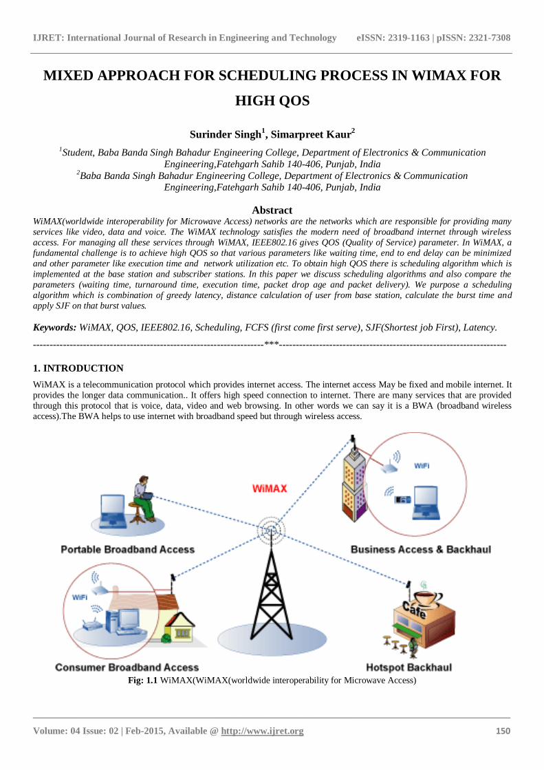
Fig: 8.4 Process number v/s utility value with greedy Latency.
Figure 8.3 shows the execution time for each process for each user with greedy latency Scheduler. The execution time for each
user shown by (*) on the graph. The graph also gives the total execution time for all process. The burst value for each user is the given values in the program. The values of burst time for each process are shown in the parameter table.
Figure 8.4 shows the utility values for each process of each user with greedy latency scheduler. The utility value for each user
shown by (*) on the graph. The utility value can be calculated with utility function of greedy latency scheduler. The utility values
are the ratio of max value of dk/tk .
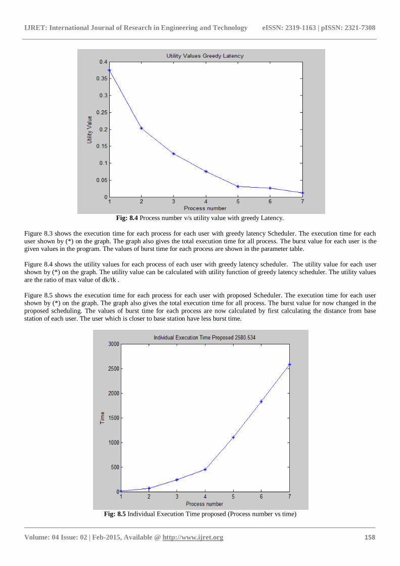
Figure 8.5 shows the execution time for each process for each user with proposed Scheduler. The execution time for each user
shown by (*) on the graph. The graph also gives the total execution time for all process. The burst value for now changed in the
proposed scheduling. The values of burst time for each process are now calculated by first calculating the distance from base
station of each user. The user which is closer to base station have less burst time.
Fig: 8.5 Individual Execution Time proposed (Process number vs time)

IJRET: International Journal of Research in Engineering and Technology eISSN: 2319-1163 | pISSN: 2321-7308
_______________________________________________________________________________________
Volume: 04 Issue: 02 | Feb-2015, Available @ http://www.ijret.org 159
Fig: 8.6 Process number v/s utility value (proposed).
Fig: 8.7 Burst time v/s Process (SJF Utility allotment)
Figure 8.6 shows the utility values for each process of each user with proposed scheduler. The utility value for each user shown
by (*) on the graph. The utility value can be calculated with utility function of greedy latency scheduler. The utility values are the
ratio of max value of dk/tk .
Figure 8.7 shows the SJF (shortest job first) of burst values for proposed algorithm. The allotment of job for each user shown by
(*) on the graph. The burst values are calculated by the proposed algorithm. In SJF algorithm the user having less burst time can
execute first and so on. It will have the great impact on the total execution time.

IJRET: International Journal of Research in Engineering and Technology eISSN: 2319-1163 | pISSN: 2321-7308
_______________________________________________________________________________________
Volume: 04 Issue: 02 | Feb-2015, Available @ http://www.ijret.org 160
Figure 8.8 shows the comparison of packet delivery/drop age of greedy latency scheduling and proposed algorithm. The
comparison of packet delivery/drop age of greedy latency with proposed algorithm scheduling for each user shown by (*) with
blue line on the graph. The comparison of packet delivery/drop age of proposed scheduling with greedy latency for each user
shown by (*) with red line on the graph. The packet delivery is more in proposed scheduling
Fig: 8.8 Packet delivery v/s process (Comparison packet delivery/dropage)
Fig: 8.9 Comparison of execution time of Greedy Latency and proposed Algorithm

IJRET: International Journal of Research in Engineering and Technology eISSN: 2319-1163 | pISSN: 2321-7308
_______________________________________________________________________________________
Volume: 04 Issue: 02 | Feb-2015, Available @ http://www.ijret.org 161
Fig: 8.10 Comparison of Average waiting time of Greedy Latency and proposed Algorithm
Fig: 8.11 Comparison of Average turnaround time of Greedy Latency and proposed Algorithm
Figure 8.10 shows the comparison of average waiting time greedy latency scheduling and proposed algorithm. The average
waiting time is less in proposed scheduling
Figure 8.11 shows the comparison of average turnaround time greedy latency scheduling and proposed algorithm The comparison
of average turnaround time time of proposed algorithm scheduling with greedy latency for each user shown by the pie chart in
GUI Interface with yellow color on the graph. The average turnaround time is less in proposed scheduling.

IJRET: International Journal of Research in Engineering and Technology eISSN: 2319-1163 | pISSN: 2321-7308
_______________________________________________________________________________________
Volume: 04 Issue: 02 | Feb-2015, Available @ http://www.ijret.org 162
Table 7.3 Simulation Results for Greedy Latency
User
number
Serial order of
process
Name of
Process
Greedy
Latency
Utility
Value
Waiting
Time
Packet
Arrival
Time
Packet
Latency
Maximum
admissible
Latency
Burst
Time
5 1 Web browsing 0.375 0 34 60 160 51
6 2
Video
Streaming 0.2025 51 22 79 400 220
2 2
Video
Streaming 0.1275 271 57 51 400 220
4 4
Media
download 0.076 491 2 76 1000 684
1 1 Web browsing 0.0313 1175 13 5 160 51
7 3 Gaming 0.026 1226 84 26 1000 770
3 3 Gaming 0.012 1996 42 12 1000 770
Table 7.4 Simulation Results for Proposed Algorithm
User
number
Serial
order
of
process
Name of
Process
Greedy
Latency
Utility
Value
Waiting
Time
Packet
Arrival
Time
Packet
Latency
Maximum
admissible
Latency
Burst
Time
Distance
from Base
station
5 1
Web
browsing 0.0264 0 0.5785 93.4215 160 17.5785 33.4215
1 1
Web
browsing 0.5839 17.5785 3.7805 4.2195 160 41.7805 9.2195
6 2
Video
Streaming 0.0917 59.359 -18.03 121.025 400 179.975 40.025
2 2
Video
Streaming 0.3026 239.334 42.682 36.6822 400 205.6822 14.3178
4 4
Media
download 0.1024 445.016 -24.42 102.4197 1000 657.5803 26.4197
7 3 Gaming 0.0697 1102.6 40.319 69.6807 1000 726.3193 43.6807
3 3 Gaming 0.0341 1828.92 19.909 34.0907 1000 747.9093 22.0907
Table 7.5 Simulation Results for Greedy Latency and Proposed Algorithm
S.NO Algorithm Average Turnaround Time Average Waiting Time Total Execution Time
1 Greedy Latency 1139.4286 744.2857 2766
2 Proposed 894.8177 526.7698 2576.3353
9. CONCLUSION AND SCOPE
The scheduling, in general help to manage so many tasks so
that time can be managed to get maximum output in real
life. Similarly if we consider the WiMAX the scheduling
can play an important role to achieve high QoS. As the
demand of high speed wireless broadband internet can
increased day by day, the no of user for using the internet
can also be increased day by day. To achieve these two
goals the scheduling plays an important role. The scheduling
algorithm will help to schedule the packet delivery for each
user and hence the speed of execution can also be increased. The scheduling algorithm said to be efficient if turnaround
time, waiting time, packet drop can be minimized. We
design the new approach for scheduling and also we can
compare all parameters of proposed algorithm with greedy
latency algorithm. In our approach the execution time for all
the processes are less as compare to the greedy latency
algorithm. Results from our simulations using MATLAB
shows that the proposed system provides a efficient
scheduling algorithm. The results shows that the average
turnaround time, waiting time and the burst time for each
process can be reduced. This will help to increase the speed
of packet delivery from base station to subscriber station.
This scheduling can increase the execution of those users
which are closer to the base station.
Future work can add more parameters like throughput of the
network. It can also be impalement to the user which is
residing more closely to the base station. As the demand of
high speed broadband internet increased day by day so this
approach will help increase the speed of execution for high
traffic environment. This approach can be applied where the
base station are closer to the users.

IJRET: International Journal of Research in Engineering and Technology eISSN: 2319-1163 | pISSN: 2321-7308
_______________________________________________________________________________________
Volume: 04 Issue: 02 | Feb-2015, Available @ http://www.ijret.org 163
REFERENCES
[1]. Andrews M., Kumaran K., Ramanan K., Stolyar A., and
Whiting P., Feb 2001 “Providing Quality of Service over a
Shared Wireless Link” IEEE Communications
Magazine,Vol.01, pp.150-154.
[2]. Agarwal M. and Puri A. 2002 “Base station scheduling
of requests with fixed deadlines” IEEE INFOCOM , Vol .02 pp . 488-496.
[3]. Anas F. Bayan and Wan T. 2010 “A Scalable QOS
Scheduling Architecture for WiMAX Multi- Hop Relay
Networks” 2nd International Conference on Education
Technology and Computer (ICETC) pp 326-331.
[4]. Ali1 D. M., and K. Dimyati 2011 “Performance
Analysis of Delay Jitter in Mobile WiMAX Systems 2011
International Conference on Information and Electronics
Engineering Vol.6 , Singapore pp 1 -5.
[5]. Ali D. and Dimyati K. July 2011 “Threshold based
Cyclic Polling (TbCP): An Uplink Scheduling Algorithm for
Mobile WiMAX Systems” International Journal of Information and Electronics Engineering, Vol. 1 , No. 1 , pp
1-8.
[6]. Al-Howaide A.,Doulat A,Yaser M. and Khamayseh
October 2011 “performance evaluation of different
scheduling algorithms in wimax” International Journal of
Computer Science, Engineering and Applications (IJCSEA)
Vol.1, No.5, pp81-94.
[7]. Ahmed M. Shabani H. Beg M. and Khader A. April
2012 “ Survey of DownLink Data Allocation Algorithms in
IEEE 802.16 WiMAX” IRACST – International Journal of
Computer Networks and Wireless Communications (IJCNWC), ISSN: 2250-3501Vol.2, No.2, pp 293-299.
[8]. Alizadeh M. ,Dziyauddin R.∗, Kaleshi D. and Doufexi
A. 2012 “A comparative study of mixed traffic scenarios for
different scheduling algorithms in WiMAX” IEEE 978-1-
4673-0990 pp 1-6.
[9]. Awan K.,Abdullah A. and Qureshi K. 2013 “Resource
Allocation in IEEE 802.16e Mobile WiMAX Networks:
Survey” World Applied Sciences Journal 28 ISSN 1818-
4952 IDOSI Publications, pp103-113.
[10] Anouari T. and Haqiq A. March 2014 “A QoE-Based
Scheduling Algorithm for UGS Service Class in WiMAX” Network International Journal of Soft Computing and
Engineering (IJSCE) ISSN: 2231-2307, Volume-4, Issue-1,
pp195-199.
[11]. BINI E. and BUTTAZZO G. 2005 “Measuring the
Performance of Schedulability Tests” Springer Science, Vol
.30 pp. 129-153.
[12]. Chandur P., Karthik R. and Sivalingam K. 2012
“Performance Evaluation of Scheduling Algorithms for
Mobile WiMAX Networks” IEEE 978-1-4673-0906-6 pp
770-775.
[13]. Chen J.,W. Jiao and H. Wang, 2005 “A service flow
management strategy for IEEE 802.16 broadband wireless access systems in tdd mode in Communications” ICC IEEE
International Conference , vol. 5, pp. 3422–3426.
[14]. Dahmouni H., El Ghazi H., Bonacci D., Sansò B. and
Girard A. MAY 2010 “Imprvoing QoS of all-IP Generation
of Pre-WiMax Networks Using Delay-Jitter Model” Journal
of telecommunications, VOL. 2, pp 99-103
[15]. Deepak H., and Nayak S. 2012,“Bandwidth Recycling
in WiMAX Networks” (IJCSIT) International Journal of
Computer Science and Information Technologies, Vol.
3,3852-3855.ISSN:0975-9646, pp.3852-3855.
[16]. Dosciatti R., Godoy W., and Foronda A., 2012 “An
efficient approach of scheduling with call admission control to fixed wimax networks,” Latin America Transactions,
IEEE (Revista IEEE America Latina), vol. 10, no. 1, pp.
1256–1264,.
[17]. Gidlund M. and Wang G MARCH 2009 “Uplink
Scheduling Algorithms for QoS Support in Broadband
Wireless Access Networks” JOURNAL OF
COMMUNICATIONS, VOL. 4,pp 133-142.
[18]. Galshetwar G., Jayakumar A. and Mittal Y. Apr 2012
“Comparative Study Of Different Scheduling Algorithms
For Wimax MAC Scheduler Design” International Journal
of Engineering Research and Applications (IJERA) ISSN: 2248-9622 Vol. 2, Issue 2, pp.1031-1037.
[19]. Gupta S. 2013 “Comparison of Various Scheduling
Algorithms in WiMAX: A Brief Review” Published in
International Journal of Computer Applications (IJCA), pp
34-36.
[20]. Haghani E. and Ansari N. 2008 “VoIP Traffic
Scheduling in WiMAX Networks”, IEEE 978-1-4244-2324
pp 1-8.
[21]. Kaur H. and Singh G. September 2011
“Implementation and Evaluation of Scheduling
Algorithmsin Point-to-Multipoint Mode in Wimax
Networks” IJCST Vol. 2, Issue 3, I S S N : 2 2 2 9 - 4 3 3 3 pp 540-546.
[22]. Kishor L. and Goyal D. April 2013 “Time Quantum
Based Improved Scheduling Algorithm”International
Journal of Advanced Research in Computer Science and
Software Engineering Volume 3, Issue 4, ISSN: 2277 128X
[23]. Khatkar A. 2013 “Performance Analysis of UGS and
BE QoS classes in WiMAX” Advance in Electronic and
Electric Engineering. ISSN 2231-1297, Volume 3, Number
7, pp. 805-810.