Embed Size (px)
Citation preview
Manufacturing Systems Modeling and Analysis
Guy L. Curry · Richard M. Feldman
Manufacturing SystemsModeling and Analysis
123
Prof. Guy L. CurryTexas A & M UniversityDept. Industrial & SystemsEngineering3131 TAMUCollege Station [email protected]
Texas A & M UniversityDept. Industrial & SystemsEngineering3131 TAMUCollege Station [email protected]
ISBN: 978-3-540-88762-1 e-ISBN: 978-3-540-88763-8
DOI 10.1007/978-3-540-88763-8
Library of Congress Control Number: 2008939370
c© Springer-Verlag Berlin Heidelberg 2009
This work is subject to copyright. All rights are reserved, whether the whole or part of the material isconcerned, specifically the rights of translation, reprinting, reuse of illustrations, recitation, broadcasting,reproduction on microfilm or in any other way, and storage in data banks. Duplication of this publicationor parts thereof is permitted only under the provisions of the German Copyright Law of September 9,1965, in its current version, and permission for use must always be obtained from Springer. Violations areliable to prosecution under the German Copyright Law.
The use of general descriptive names, registered names, trademarks, etc. in this publication does not imply,even in the absence of a specific statement, that such names are exempt from the relevant protective lawsand regulations and therefore free for general use.
Cover design: eStudio Calamar S.L.
Printed on acid-free paper
9 8 7 6 5 4 3 2 1
springer.com
Prof. Richard M. Feldman
This book is dedicated to the two individualswho keep us going, tolerate our work ethic,and make life a wondrous journey, our wives:Jerrie Curry and Alice Feldman.
Preface
This textbook was developed to fill the need for an accessible but comprehensivepresentation of the analytical approaches for modeling and analyzing models ofmanufacturing and production systems. It is an out growth of the efforts withinthe Industrial and Systems Engineering Department at Texas A&M to develop andteach an analytically based undergraduate course on probabilistic modeling of man-ufacturing type systems. The level of this textbook is directed at undergraduate andmasters students in engineering and mathematical sciences. The only prerequisitefor students using this textbook is a previous course covering calculus-based prob-ability and statistics. The underlying methodology is queueing theory, and we shalldevelop the basic concepts in queueing theory in sufficient detail that the readerneed not have previously covered it. Queueing theory is a well-established disci-pline dating back to the early 1900’s work of A. K. Erlang, a Danish mathematician,on telephone traffic congestion. Although there are many textbooks on queueingtheory, these texts are generally oriented to the methodological development of thefield and exact results and not to the practical application of using approximationsin realistic modeling situations. The application of queueing theory to manufactur-ing type systems started with the approximation based work of Ward Whitt in the1980’s. His paper on QNA (a queueing network analyzer) in 1983 is the base fromwhich most applied modeling efforts have evolved.
There are several textbooks with titles similar to this book. Principle amongthese are: Modeling and Analysis of Manufacturing Systems by Askin and Stan-dridge, Manufacturing Systems Engineering by Stanley Gershwin, Queueing The-ory in Manufacturing Systems Analysis and Design by Papadopoulos, Heaveyand Browne, Performance Analysis of Manufacturing Systems by Tayfur Altiok,Stochastic Modeling and Analysis of Manufacturing Systems, edited by David Yao,and Stochastic Models of Manufacturing Systems by Buzacott and Shanthikumar.Each of these texts, along with several others, contributes greatly to the field. Thebook that most closely aligns with the motivation, level, and intent of this bookis Factory Physics by Hopp and Spearman. Their approach and analysis is highlyrecommended reading, however, their book’s scope is on the larger field of produc-
vii
viii Preface
tion and operations management. Thus, it does not provide the depth and breath ofanalytical modeling procedures that are presented in this text.
This text is about the development of analytical approximation models and theiruse in evaluating factory performance. The tools needed for the analytical approachare fully developed. One useful non-analytical tool that is not fully developed inthis textbook is simulation modeling. In practice as well as in the development ofthe models in this text, simulation is extensively used as a verification tool. Eventhough the development of simulation models is only modestly addressed, we wouldencourage instructors who use this book in their curriculum after a simulation courseto ask students to simulate some of the homework problems so that a comparisoncan be made of the analysis using the models presented here with simulation mod-els. By developing simulation models students will have a better understanding ofthe modeling assumptions and the accuracy of the analytical approximations. In ad-dition several chapters include an appendix that contains instructions in the use ofMicrosoft Excel as an aid in modeling or in building simple simulation models.
Two special sections are included to help the reader organize the many conceptscontained in the text. Immediately after the Table of Contents, we have included asymbol table that contains most of the notation used throughout the text. Second,immediately after the final chapter a glossary of terms is included that summarizesthe various definitions used. It is expected that these will prove valuable resourcesas the reader progresses through the text.
Many individuals have contributed to this book through our interactions in re-search efforts and discussions. Special thanks go to Professor Martin A. Wortman,Texas A&M University, who designed and taught the first presentation of the coursefor which this book was originally developed and Professor Bryan L. Deuermeyer,Texas A&M University, for his significant contributions to our joint research ac-tivities in this area and his continued interest and criticism. In addition several in-dividuals have helped in improving the text by using a draft copy while teachingthe material to undergraduates including Eylem Tekin at Texas A&M, NatarajanGautam also at Texas A&M, and Kevin Gue at Auburn University. We also wish toacknowledge the contributions of Professors John A. Fowler, Arizona State Univer-sity, and Mark L. Spearman, Factory Physics, Inc., for their continued interactionsand discussions on modeling manufacturing systems. And we thank Ciriaco Valdez-Flores, a co-author of the first chapter covering basic probability for permission toinclude it as part of our book. Finally, we acknowledge our thanks through the wordsof the psalmist, “Give thanks to the Lord, for He is good; His love endures forever.”(Psalms 107:1, NIV)
College Station, Texas Guy L. CurryRichard M. FeldmanDecember 2008

Contents
1 Basic Probability Review . . . . . . . . . . . . . . . . . . . . . . . . . . . . . . . . . . . . . . . . 11.1 Basic Definitions . . . . . . . . . . . . . . . . . . . . . . . . . . . . . . . . . . . . . . . . . . . 11.2 Random Variables and Distribution Functions . . . . . . . . . . . . . . . . . . . 41.3 Mean and Variance . . . . . . . . . . . . . . . . . . . . . . . . . . . . . . . . . . . . . . . . . 101.4 Important Distributions . . . . . . . . . . . . . . . . . . . . . . . . . . . . . . . . . . . . . . 131.5 Multivariate Distributions . . . . . . . . . . . . . . . . . . . . . . . . . . . . . . . . . . . . 231.6 Combinations of Random Variables . . . . . . . . . . . . . . . . . . . . . . . . . . . 31
1.6.1 Fixed Sum of Random Variables . . . . . . . . . . . . . . . . . . . . . . . 311.6.2 Random Sum of Random Variables . . . . . . . . . . . . . . . . . . . . . 321.6.3 Mixtures of Random Variables . . . . . . . . . . . . . . . . . . . . . . . . . 34
Appendix . . . . . . . . . . . . . . . . . . . . . . . . . . . . . . . . . . . . . . . . . . . . . . . . . . . . . . 35Problems . . . . . . . . . . . . . . . . . . . . . . . . . . . . . . . . . . . . . . . . . . . . . . . . . . . . . . 36References . . . . . . . . . . . . . . . . . . . . . . . . . . . . . . . . . . . . . . . . . . . . . . . . . . . . . 43
2 Introduction to Factory Models . . . . . . . . . . . . . . . . . . . . . . . . . . . . . . . . . . 452.1 The Basics . . . . . . . . . . . . . . . . . . . . . . . . . . . . . . . . . . . . . . . . . . . . . . . . 45
2.1.1 Notation, Definitions and Diagrams . . . . . . . . . . . . . . . . . . . . . 462.1.2 Measured Data and System Parameters . . . . . . . . . . . . . . . . . . 49
2.2 Introduction to Factory Performance . . . . . . . . . . . . . . . . . . . . . . . . . . . 542.2.1 The Modeling Method . . . . . . . . . . . . . . . . . . . . . . . . . . . . . . . . 552.2.2 Model Usage . . . . . . . . . . . . . . . . . . . . . . . . . . . . . . . . . . . . . . . . 582.2.3 Model Conclusions . . . . . . . . . . . . . . . . . . . . . . . . . . . . . . . . . . . 59
2.3 Deterministic vs Stochastic Models . . . . . . . . . . . . . . . . . . . . . . . . . . . 60Appendix . . . . . . . . . . . . . . . . . . . . . . . . . . . . . . . . . . . . . . . . . . . . . . . . . . . . . . 62Problems . . . . . . . . . . . . . . . . . . . . . . . . . . . . . . . . . . . . . . . . . . . . . . . . . . . . . . 65References . . . . . . . . . . . . . . . . . . . . . . . . . . . . . . . . . . . . . . . . . . . . . . . . . . . . . 67
3 Single Workstation Factory Models . . . . . . . . . . . . . . . . . . . . . . . . . . . . . . 693.1 First Model . . . . . . . . . . . . . . . . . . . . . . . . . . . . . . . . . . . . . . . . . . . . . . . . 693.2 Diagram Method for Developing the Balance Equations . . . . . . . . . . 733.3 Model Shorthand Notation . . . . . . . . . . . . . . . . . . . . . . . . . . . . . . . . . . . 76
ix
x Contents
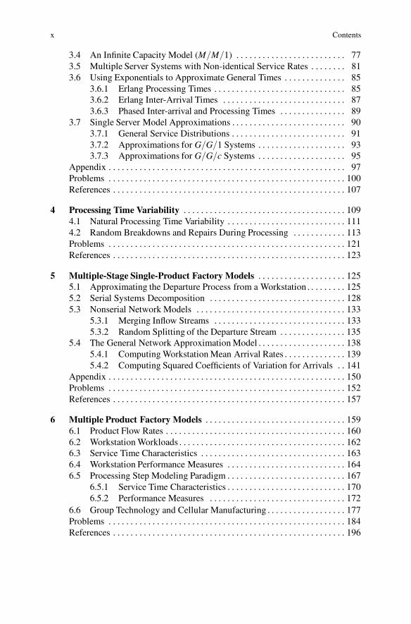
3.4 An Infinite Capacity Model (M/M/1) . . . . . . . . . . . . . . . . . . . . . . . . . 773.5 Multiple Server Systems with Non-identical Service Rates . . . . . . . . 813.6 Using Exponentials to Approximate General Times . . . . . . . . . . . . . . 85
3.6.1 Erlang Processing Times . . . . . . . . . . . . . . . . . . . . . . . . . . . . . . 853.6.2 Erlang Inter-Arrival Times . . . . . . . . . . . . . . . . . . . . . . . . . . . . 873.6.3 Phased Inter-arrival and Processing Times . . . . . . . . . . . . . . . 89
3.7 Single Server Model Approximations . . . . . . . . . . . . . . . . . . . . . . . . . . 903.7.1 General Service Distributions . . . . . . . . . . . . . . . . . . . . . . . . . . 913.7.2 Approximations for G/G/1 Systems . . . . . . . . . . . . . . . . . . . . 933.7.3 Approximations for G/G/c Systems . . . . . . . . . . . . . . . . . . . . 95
Appendix . . . . . . . . . . . . . . . . . . . . . . . . . . . . . . . . . . . . . . . . . . . . . . . . . . . . . . 97Problems . . . . . . . . . . . . . . . . . . . . . . . . . . . . . . . . . . . . . . . . . . . . . . . . . . . . . . 100References . . . . . . . . . . . . . . . . . . . . . . . . . . . . . . . . . . . . . . . . . . . . . . . . . . . . . 107
4 Processing Time Variability . . . . . . . . . . . . . . . . . . . . . . . . . . . . . . . . . . . . . 1094.1 Natural Processing Time Variability . . . . . . . . . . . . . . . . . . . . . . . . . . . 1114.2 Random Breakdowns and Repairs During Processing . . . . . . . . . . . . 113Problems . . . . . . . . . . . . . . . . . . . . . . . . . . . . . . . . . . . . . . . . . . . . . . . . . . . . . . 121References . . . . . . . . . . . . . . . . . . . . . . . . . . . . . . . . . . . . . . . . . . . . . . . . . . . . . 123
5 Multiple-Stage Single-Product Factory Models . . . . . . . . . . . . . . . . . . . . 1255.1 Approximating the Departure Process from a Workstation . . . . . . . . . 1255.2 Serial Systems Decomposition . . . . . . . . . . . . . . . . . . . . . . . . . . . . . . . 1285.3 Nonserial Network Models . . . . . . . . . . . . . . . . . . . . . . . . . . . . . . . . . . 133
5.3.1 Merging Inflow Streams . . . . . . . . . . . . . . . . . . . . . . . . . . . . . . 1335.3.2 Random Splitting of the Departure Stream . . . . . . . . . . . . . . . 135
5.4 The General Network Approximation Model . . . . . . . . . . . . . . . . . . . . 1385.4.1 Computing Workstation Mean Arrival Rates . . . . . . . . . . . . . . 1395.4.2 Computing Squared Coefficients of Variation for Arrivals . . 141
Appendix . . . . . . . . . . . . . . . . . . . . . . . . . . . . . . . . . . . . . . . . . . . . . . . . . . . . . . 150Problems . . . . . . . . . . . . . . . . . . . . . . . . . . . . . . . . . . . . . . . . . . . . . . . . . . . . . . 152References . . . . . . . . . . . . . . . . . . . . . . . . . . . . . . . . . . . . . . . . . . . . . . . . . . . . . 157
6 Multiple Product Factory Models . . . . . . . . . . . . . . . . . . . . . . . . . . . . . . . . 1596.1 Product Flow Rates . . . . . . . . . . . . . . . . . . . . . . . . . . . . . . . . . . . . . . . . . 1606.2 Workstation Workloads . . . . . . . . . . . . . . . . . . . . . . . . . . . . . . . . . . . . . . 1626.3 Service Time Characteristics . . . . . . . . . . . . . . . . . . . . . . . . . . . . . . . . . 1636.4 Workstation Performance Measures . . . . . . . . . . . . . . . . . . . . . . . . . . . 1646.5 Processing Step Modeling Paradigm . . . . . . . . . . . . . . . . . . . . . . . . . . . 167
6.5.1 Service Time Characteristics . . . . . . . . . . . . . . . . . . . . . . . . . . . 1706.5.2 Performance Measures . . . . . . . . . . . . . . . . . . . . . . . . . . . . . . . 172
6.6 Group Technology and Cellular Manufacturing . . . . . . . . . . . . . . . . . . 177Problems . . . . . . . . . . . . . . . . . . . . . . . . . . . . . . . . . . . . . . . . . . . . . . . . . . . . . . 184References . . . . . . . . . . . . . . . . . . . . . . . . . . . . . . . . . . . . . . . . . . . . . . . . . . . . . 196
Contents xi
7 Models of Various Forms of Batching . . . . . . . . . . . . . . . . . . . . . . . . . . . . . 1977.1 Batch Moves . . . . . . . . . . . . . . . . . . . . . . . . . . . . . . . . . . . . . . . . . . . . . . 198
7.1.1 Batch Forming Time . . . . . . . . . . . . . . . . . . . . . . . . . . . . . . . . . 1997.1.2 Batch Queue Cycle Time . . . . . . . . . . . . . . . . . . . . . . . . . . . . . . 2017.1.3 Batch Move Processing Time Delays . . . . . . . . . . . . . . . . . . . . 2027.1.4 Inter-departure Time SCV with Batch Move Arrivals . . . . . . 204
7.2 Batching for Setup Reduction . . . . . . . . . . . . . . . . . . . . . . . . . . . . . . . . 2067.2.1 Inter-departure Time SCV with Batch Setups . . . . . . . . . . . . . 209
7.3 Batch Service Model . . . . . . . . . . . . . . . . . . . . . . . . . . . . . . . . . . . . . . . . 2097.3.1 Cycle Time for Batch Service . . . . . . . . . . . . . . . . . . . . . . . . . . 2107.3.2 Departure Process for Batch Service . . . . . . . . . . . . . . . . . . . . 211
7.4 Modeling the Workstation Following a Batch Server . . . . . . . . . . . . . 2137.4.1 A Serial System Topology . . . . . . . . . . . . . . . . . . . . . . . . . . . . . 2137.4.2 Branching Following a Batch Server . . . . . . . . . . . . . . . . . . . . 214
7.5 Batch Network Examples . . . . . . . . . . . . . . . . . . . . . . . . . . . . . . . . . . . . 2227.5.1 Batch Network Example 1 . . . . . . . . . . . . . . . . . . . . . . . . . . . . . 2227.5.2 Batch Network Example 2 . . . . . . . . . . . . . . . . . . . . . . . . . . . . . 226
Problems . . . . . . . . . . . . . . . . . . . . . . . . . . . . . . . . . . . . . . . . . . . . . . . . . . . . . . 230References . . . . . . . . . . . . . . . . . . . . . . . . . . . . . . . . . . . . . . . . . . . . . . . . . . . . . 240
8 WIP Limiting Control Strategies . . . . . . . . . . . . . . . . . . . . . . . . . . . . . . . . . 2418.1 Closed Queueing Networks for Single Products . . . . . . . . . . . . . . . . . 242
8.1.1 Analysis with Exponential Processing Times . . . . . . . . . . . . . 2458.1.2 Analysis with General Processing Times . . . . . . . . . . . . . . . . . 252
8.2 Closed Queueing Networks with Multiple Products . . . . . . . . . . . . . . 2558.2.1 Mean Value Analysis for Multiple Products . . . . . . . . . . . . . . 2568.2.2 Mean Value Analysis Approximation for Multiple Products . 2608.2.3 General Service Time Approximation for Multiple
Products . . . . . . . . . . . . . . . . . . . . . . . . . . . . . . . . . . . . . . . . . . . 2628.3 Production and Sequencing Strategies . . . . . . . . . . . 267
8.3.1 Problem Statement . . . . . . . . . . . . . . . . . . . . . . . . . . . . . . . . . . . 2688.3.2 Push Strategy Model . . . . . . . . . . . . . . . . . . . . . . . . . . . . . . . . . 2698.3.3 CONWIP Strategy Model . . . . . . . . . . . . . . . . . . . . . . . . . . . . . 271
Appendix . . . . . . . . . . . . . . . . . . . . . . . . . . . . . . . . . . . . . . . . . . . . . . . . . . . . . . 272Problems . . . . . . . . . . . . . . . . . . . . . . . . . . . . . . . . . . . . . . . . . . . . . . . . . . . . . . 273References . . . . . . . . . . . . . . . . . . . . . . . . . . . . . . . . . . . . . . . . . . . . . . . . . . . . . 279
9 Serial Limited Buffer Models . . . . . . . . . . . . . . . . . . . . . . . . . . . . . . . . . . . . 2819.1 The Decomposition Approach used for Kanban Systems . . . . . . . . . . 2829.2 Modeling The Two-Node Subsystem . . . . . . . . . . . . . . . . . . . . . . . . . . 284
9.2.1 Modeling the Service Distribution . . . . . . . . . . . . . . . . . . . . . . 285
: A case study . . .
9.2.2 Structure of the State-Space . . . . . . . . . . . . . . . . . . . . . . . . . . . 2889.2.3 Generator Matrix Relating System Probabilities . . . . . . . . . . . 2909.2.4 Connecting the Subsystems . . . . . . . . . . . . . . . . . . . . . . . . . . . . 291
xii Contents
9.3 Example of a Kanban Serial System . . . . . . . . . . . . . . . . . . . . . . . . . . . 2939.3.1 The First Forward Pass . . . . . . . . . . . . . . . . . . . . . . . . . . . . . . . 2949.3.2 The Backward Pass . . . . . . . . . . . . . . . . . . . . . . . . . . . . . . . . . . 3009.3.3 The Remaining Iterations . . . . . . . . . . . . . . . . . . . . . . . . . . . . . 3079.3.4 Convergence and Factory Performance Measures . . . . . . . . . 3089.3.5 Generalizations . . . . . . . . . . . . . . . . . . . . . . . . . . . . . . . . . . . . . . 310
9.4 Setting Kanban Limits . . . . . . . . . . . . . . . . . . . . . . . . . . . . . . . . . . . . . . 3109.4.1 Allocating a Fixed Number of Buffer Units . . . . . . . . . . . . . . 3119.4.2 Cycle Time Restriction . . . . . . . . . . . . . . . . . . . . . . . . . . . . . . . 3159.4.3 Serial Factory Results . . . . . . . . . . . . . . . . . . . . . . . . . . . . . . . . 316
Problems . . . . . . . . . . . . . . . . . . . . . . . . . . . . . . . . . . . . . . . . . . . . . . . . . . . . . . 317References . . . . . . . . . . . . . . . . . . . . . . . . . . . . . . . . . . . . . . . . . . . . . . . . . . . . . 320
Glossary . . . . . . . . . . . . . . . . . . . . . . . . . . . . . . . . . . . . . . . . . . . . . . . . . . . . . . . . . . 321
Index . . . . . . . . . . . . . . . . . . . . . . . . . . . . . . . . . . . . . . . . . . . . . . . . . . . . . . . . . . . . . 325
Symbols
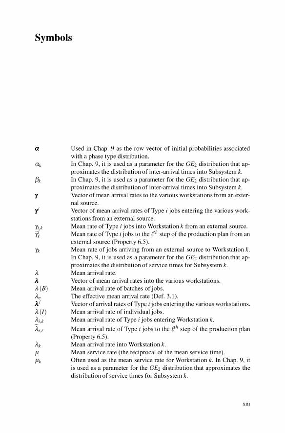
ααα Used in Chap. 9 as the row vector of initial probabilities associatedwith a phase type distribution.
αk In Chap. 9, it is used as a parameter for the GE2 distribution that ap-proximates the distribution of inter-arrival times into Subsystem k.
βk In Chap. 9, it is used as a parameter for the GE2 distribution that ap-proximates the distribution of inter-arrival times into Subsystem k.
γγγ Vector of mean arrival rates to the various workstations from an exter-nal source.
γγγ i Vector of mean arrival rates of Type i jobs entering the various work-stations from an external source.
γi,k Mean rate of Type i jobs into Workstation k from an external source.˜γ i� Mean rate of Type i jobs to the �th step of the production plan from an
external source (Property 6.5).γk Mean rate of jobs arriving from an external source to Workstation k.
In Chap. 9, it is used as a parameter for the GE2 distribution that ap-proximates the distribution of service times for Subsystem k.
λ Mean arrival rate.λλλ Vector of mean arrival rates into the various workstations.λ (B) Mean arrival rate of batches of jobs.λe The effective mean arrival rate (Def. 3.1).λλλ i Vector of arrival rates of Type i jobs entering the various workstations.λ (I) Mean arrival rate of individual jobs.λi,k Mean arrival rate of Type i jobs entering Workstation k.˜λi,� Mean arrival rate of Type i jobs to the �th step of the production plan
(Property 6.5).λk Mean arrival rate into Workstation k.μ Mean service rate (the reciprocal of the mean service time).μk Often used as the mean service rate for Workstation k. In Chap. 9, it
is used as a parameter for the GE2 distribution that approximates thedistribution of service times for Subsystem k.
xiii
xiv Symbols
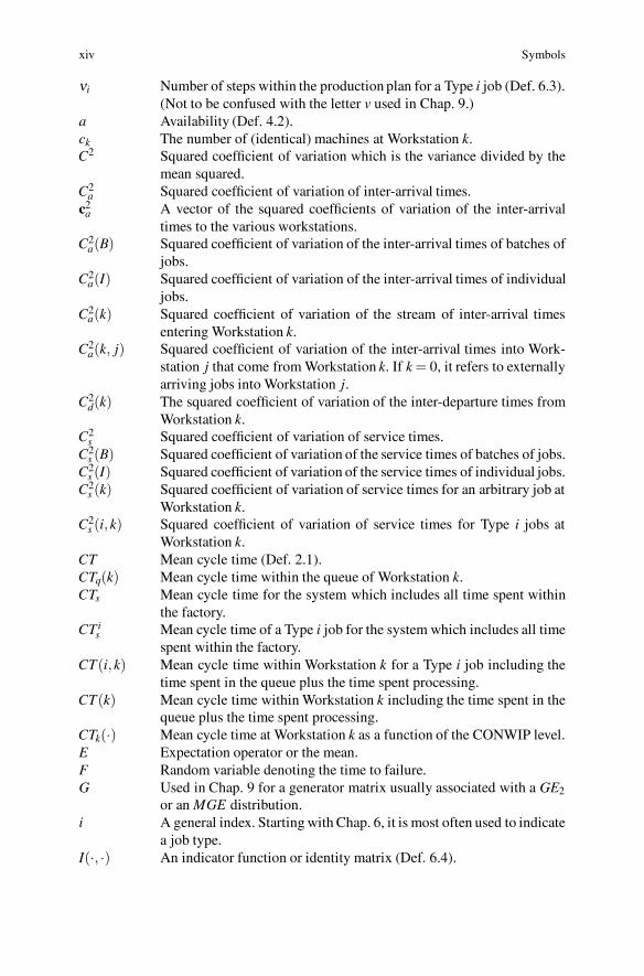
νi Number of steps within the production plan for a Type i job (Def. 6.3).(Not to be confused with the letter v used in Chap. 9.)
a Availability (Def. 4.2).ck The number of (identical) machines at Workstation k.C2 Squared coefficient of variation which is the variance divided by the
mean squared.C2
a Squared coefficient of variation of inter-arrival times.c2
a A vector of the squared coefficients of variation of the inter-arrivaltimes to the various workstations.
C2a(B) Squared coefficient of variation of the inter-arrival times of batches of
jobs.C2
a(I) Squared coefficient of variation of the inter-arrival times of individualjobs.
C2a(k) Squared coefficient of variation of the stream of inter-arrival times
entering Workstation k.C2
a(k, j) Squared coefficient of variation of the inter-arrival times into Work-station j that come from Workstation k. If k = 0, it refers to externallyarriving jobs into Workstation j.
C2d(k) The squared coefficient of variation of the inter-departure times from
Workstation k.C2
s Squared coefficient of variation of service times.C2
s (B) Squared coefficient of variation of the service times of batches of jobs.C2
s (I) Squared coefficient of variation of the service times of individual jobs.C2
s (k) Squared coefficient of variation of service times for an arbitrary job atWorkstation k.
C2s (i,k) Squared coefficient of variation of service times for Type i jobs at
Workstation k.CT Mean cycle time (Def. 2.1).CTq(k) Mean cycle time within the queue of Workstation k.CTs Mean cycle time for the system which includes all time spent within
the factory.CTi
s Mean cycle time of a Type i job for the system which includes all timespent within the factory.
CT(i,k) Mean cycle time within Workstation k for a Type i job including thetime spent in the queue plus the time spent processing.
CT(k) Mean cycle time within Workstation k including the time spent in thequeue plus the time spent processing.
CTk(·) Mean cycle time at Workstation k as a function of the CONWIP level.E Expectation operator or the mean.F Random variable denoting the time to failure.G Used in Chap. 9 for a generator matrix usually associated with a GE2
or an MGE distribution.i A general index. Starting with Chap. 6, it is most often used to indicate
a job type.I(·, ·) An indicator function or identity matrix (Def. 6.4).
Symbols xv
k A general index. Starting with Chap. 6, it is most often used to indicatea workstation, and in Chap. 7 it is also used for batch size.
� A general index. Most often used to denote the �th step of a productionplan. In Chap. 8, it is sometimes used to indicate job type.
m Most often used for the total number of job types.n Most often used for the total number of workstations.N In Chap. 7, it is a random variable denoting batch size.P = (p j,k) Routing matrix (Def. 5.2).Pi = (pi
j,k) Routing matrix of Type i jobs.˜Pi = (pi
�, j) Step-wise routing matrix for Type i jobs (Def. 6.3).
pFa,n In Chap. 9, the probability that an arrival to the nth (or final) subsys-
tem, finds the subsystem full.
p(i,F)a,k In Chap. 9, the probability that an arrival to Subsystem k, for k < n,
finds the subsystem full and the service-machine in Phase i.p0
d,1 In Chap. 9, the probability that a departure from Subsystem 1 leavesthe subsystem empty.
p(i,0)d,k In Chap. 9, the probability that a departure from Subsystem k, for
k > 1, leaves the subsystem empty and the arrival-machine in Phase i.pk Often used for the steady-state probability of k jobs being within a
system. In Chap. 9, it is used as a parameter for the GE2 distributionthat approximates the distribution of inter-arrival times into Subsys-tem k.
pk( j,w) The steady-state probability that there are j jobs at Workstation kwhen the CONWIP level for the factory is set to w.
Q Used in Chap. 9 for a generator matrix usually associated with findingthe steady-state probabilities of two-node subsystems.
qk In Chap. 9, it is used as a parameter for the GE2 distribution that ap-proximates the distribution of service times for Subsystem k.
R Random variable denoting repair time, except in Chap. 7 where it isthe random variable denoting the setup time for a batch.
rk The relative arrival rate into Workstation k.Te Random variable denoting the effective service time (Def. 4.1).Ta(B) Random variable denoting inter-arrival times of batches of jobs.Ta(I) Random variable denoting inter-arrival times of individual jobs.Ts(B) Random variable denoting service times of batches of jobs.Ts(I) Random variable denoting service times of individual jobs.Ts(i,k) Random variable denoting service times for a Type i job in Worksta-
tion k.Ts(k) Random variable denoting service times for an arbitrary job in Work-
station k.th Mean throughput rate (Def. 2.3).th(k) Mean throughput rate for Workstation k.u Machine utilization.uk Utilization factor for Workstation k (Eq. (6.2).
xvi Symbols
uk(·) Utilization factor at Workstation k as a function of the CONWIP level.V The variance which also equals the second moment minus the mean
squared.v In Chap. 9, a vector of steady-state probabilities derived for a gen-
erator matrix. (Not to be confused with the Greek letter ν used inChap. 6.)
vi In Chap. 9, the steady-state probability of being in State i. (Not to beconfused with the Greek letter ν used in Chap. 6.)
w Used in Chaps. 8 and 9 as a variable for functions whose independentvariable represents work-in-process.
w A vector of dimension m, where m is the number of job types, givingthe CONWIP limits for each job type.
wmax In Chaps. 8 and 9 constant indicated a maximum limit placed on work-in-process.
wi(·) The workstation mapping function (Def. 6.2).WIP Mean (time-averaged) work-in-process (Def. 2.2).WIPq(k) Mean (time-averaged) work-in-process for the queue of Worksta-
tion k.WIPs Mean (time-averaged) work-in-process within the system which in-
cludes all jobs within the factory.WIP(k) Mean (time-averaged) work-in-process within Workstation k includ-
ing jobs in the queue and job(s) within the processor.WIPk(·) Mean (time-averaged) work-in-process at Workstation k as a function
of the CONWIP level.WLk Workload at Workstation k (Def. 6.1 and Eq. (6.1)).

Chapter 1Basic Probability Review
The background material for this textbook is a general understanding of probabilityand the properties of various distributions; thus, before discussing the modeling ofthe various manufacturing and production systems, it is important to review thefundamental concepts of basic probability. This material is not intended to teachprobability theory, but it is used for review and to establish a common ground forthe notation and definitions used throughout the book. Much of the material in thischapter is taken from [3], and for those already familiar with probability, this chaptercan easily be skipped.
1.1 Basic Definitions
To understand probability , it is best to envision an experiment for which the out-come (result) is unknown. All possible outcomes must be defined and the collectionof these outcomes is called the sample space. Probabilities are assigned to subsets ofthe sample space, called events. We shall give the rigorous definition for probability.However, the reader should not be discouraged if an intuitive understanding is notimmediately acquired. This takes time and the best way to understand probability isby working problems.
Definition 1.1. An element of a sample space is an outcome. A set of outcomes, orequivalently a subset of the sample space, is called an event.
Definition 1.2. A probability space is a three-tuple (Ω ,F ,Pr) where Ω is a samplespace, F is a collection of events from the sample space, and Pr is a probabilitymeasure that assigns a number to each event contained in F . Furthermore, Pr mustsatisfy the following conditions, for each event A,B within F :
• Pr(Ω ) = 1,• Pr(A) ≥ 0,• Pr(A∪B) = Pr(A)+Pr(B) if A∩B = φ , where φ denotes the empty set,
1
2 1 Basic Probability Review
• Pr(Ac) = 1−Pr(A), where Ac is the complement of A.
It should be noted that the collection of events, F , in the definition of a probabil-ity space must satisfy some technical mathematical conditions that are not discussedin this text. If the sample space contains a finite number of elements, then F usu-ally consists of all the possible subsets of the sample space. The four conditions onthe probability measure Pr should appeal to one’s intuitive concept of probability.The first condition indicates that something from the sample space must happen, thesecond condition indicates that negative probabilities are illegal, the third conditionindicates that the probability of the union of two disjoint (or mutually exclusive)events is the sum of their individual probabilities and the fourth condition indicatesthat the probability of an event is equal to one minus the probability of its comple-ment (all other events). The fourth condition is actually redundant but it is listed inthe definitions because of its usefulness.
A probability space is the full description of an experiment; however, it is notalways necessary to work with the entire space. One possible reason for workingwithin a restricted space is because certain facts about the experiment are alreadyknown. For example, suppose a dispatcher at a refinery has just sent a barge con-taining jet fuel to a terminal 800 miles down river. Personnel at the terminal wouldlike a prediction on when the fuel will arrive. The experiment consists of all possi-ble weather, river, and barge conditions that would affect the travel time down river.However, when the dispatcher looks outside it is raining. Thus, the original prob-ability space can be restricted to include only rainy conditions. Probabilities thusrestricted are called conditional probabilities according to the following definition.
Definition 1.3. Let (Ω ,F ,Pr) be a probability space where A and B are events inF with Pr(B) �= 0. The conditional probability of A given B, denoted Pr(A|B), is
Pr(A|B) =Pr(A∩B)
Pr(B).
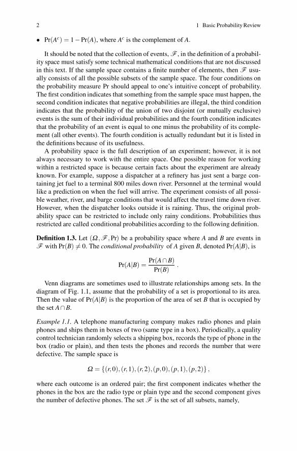
Venn diagrams are sometimes used to illustrate relationships among sets. In thediagram of Fig. 1.1, assume that the probability of a set is proportional to its area.Then the value of Pr(A|B) is the proportion of the area of set B that is occupied bythe set A∩B.
Example 1.1. A telephone manufacturing company makes radio phones and plainphones and ships them in boxes of two (same type in a box). Periodically, a qualitycontrol technician randomly selects a shipping box, records the type of phone in thebox (radio or plain), and then tests the phones and records the number that weredefective. The sample space is
Ω = {(r,0), (r,1), (r,2),(p,0),(p,1),(p,2)} ,
where each outcome is an ordered pair; the first component indicates whether thephones in the box are the radio type or plain type and the second component givesthe number of defective phones. The set F is the set of all subsets, namely,

1.1 Basic Definitions 3
Fig. 1.1 Venn diagram illus-trating events A, B, and A∩B
F = {φ ,{(r,0)},{(r,1)},{(r,0),(r,1)}, · · · ,Ω} .
There are many legitimate probability laws that could be associated with this space.One possibility is
Pr{(r,0)}= 0.45 , Pr{(p,0)}= 0.37 ,
Pr{(r,1)}= 0.07 , Pr{(p,1)}= 0.08 ,
Pr{(r,2)}= 0.01 , Pr{(p,2)}= 0.02 .
By using the last property in Definition 1.2, the probability measure can be extendedto all events; for example, the probability that a box is selected that contains radiophones and at most one phone is defective is given by
Pr{(r,0), (r,1)}= 0.52 .
Now let us assume that a box has been selected and opened. We observe that the twophones within the box are radio phones, but no test has yet been made on whetheror not the phones are defective. To determine the probability that at most one phoneis defective in the box containing radio phones, define the event A to be the set{(r,0), (r,1), (p,0), (p,1)}and the event B to be {(r,0), (r,1), (r,2)}. In other words,A is the event of having at most one defective phone, and B is the event of having abox of radio phones. The probability statement can now be written as
Pr{A|B} =Pr(A∩B)
Pr(B)=
Pr{(r,0), (r,1)}Pr{(r,0), (r,1), (r,2)} =
0.520.53
= 0.991 .
��
• Suggestion: Do Problems 1.1–1.2 and 1.20.
4 1 Basic Probability Review
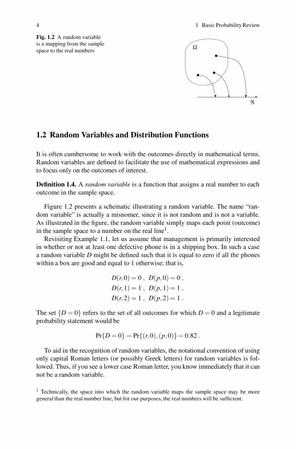
Fig. 1.2 A random variableis a mapping from the samplespace to the real numbers
Ω
ℜ
1.2 Random Variables and Distribution Functions
It is often cumbersome to work with the outcomes directly in mathematical terms.Random variables are defined to facilitate the use of mathematical expressions andto focus only on the outcomes of interest.
Definition 1.4. A random variable is a function that assigns a real number to eachoutcome in the sample space.
Figure 1.2 presents a schematic illustrating a random variable. The name “ran-dom variable” is actually a misnomer, since it is not random and is not a variable.As illustrated in the figure, the random variable simply maps each point (outcome)in the sample space to a number on the real line1.
Revisiting Example 1.1, let us assume that management is primarily interestedin whether or not at least one defective phone is in a shipping box. In such a casea random variable D might be defined such that it is equal to zero if all the phoneswithin a box are good and equal to 1 otherwise; that is,
D(r,0) = 0 , D(p,0) = 0 ,
D(r,1) = 1 , D(p,1) = 1 ,
D(r,2) = 1 , D(p,2) = 1 .
The set {D = 0} refers to the set of all outcomes for which D = 0 and a legitimateprobability statement would be
Pr{D = 0} = Pr{(r,0), (p,0)}= 0.82 .
To aid in the recognition of random variables, the notational convention of usingonly capital Roman letters (or possibly Greek letters) for random variables is fol-lowed. Thus, if you see a lower case Roman letter, you know immediately that it cannot be a random variable.
1 Technically, the space into which the random variable maps the sample space may be moregeneral than the real number line, but for our purposes, the real numbers will be sufficient.
1.2 Random Variables and Distribution Functions 5
Random variables are either discrete or continuous depending on their possiblevalues. If the possible values can be counted, the random variable is called discrete;otherwise, it is called continuous. The random variable D defined in the previousexample is discrete. To give an example of a continuous random variable, define Tto be a random variable that represents the length of time that it takes to test thephones within a shipping box. The range of possible values for T is the set of allpositive real numbers, and thus T is a continuous random variable.
A cumulative distribution function (CDF) is often used to describe the probabil-ity measure underlying the random variable. The cumulative distribution function(usually denoted by a capital Roman letter or a Greek letter) gives the probabilityaccumulated up to and including the point at which it is evaluated.
Definition 1.5. The function F is the cumulative distribution function for the ran-dom variable X if
F(a) = Pr{X ≤ a}for all real numbers a.
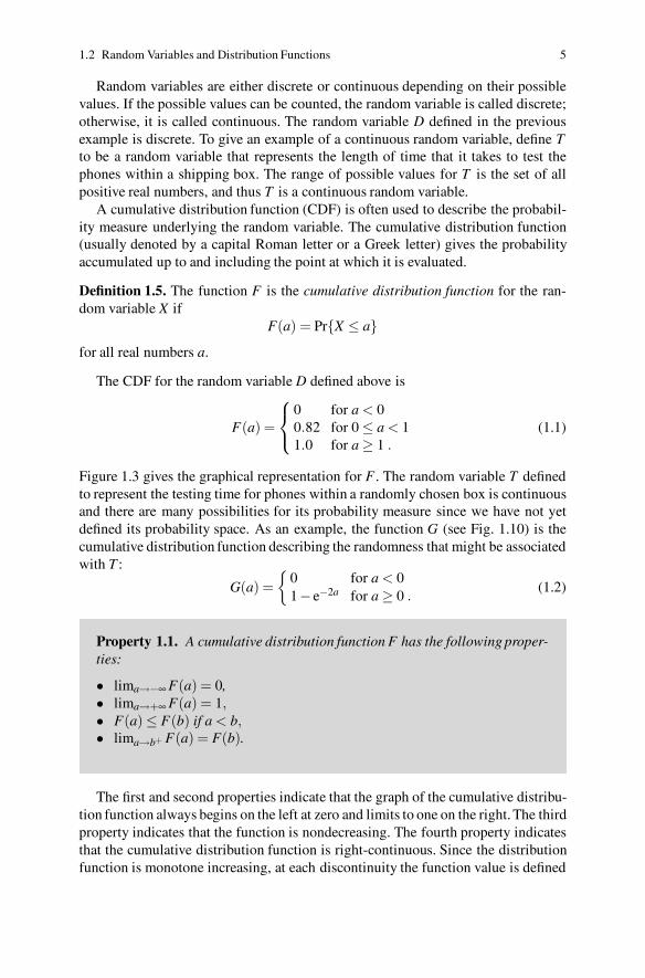
The CDF for the random variable D defined above is
F(a) =
⎧
⎨
⎩
0 for a < 00.82 for 0 ≤ a < 11.0 for a ≥ 1 .
(1.1)
Figure 1.3 gives the graphical representation for F . The random variable T definedto represent the testing time for phones within a randomly chosen box is continuousand there are many possibilities for its probability measure since we have not yetdefined its probability space. As an example, the function G (see Fig. 1.10) is thecumulative distribution function describing the randomness that might be associatedwith T :
G(a) ={
0 for a < 01− e−2a for a ≥ 0 .
(1.2)
Property 1.1. A cumulative distribution function F has the following proper-ties:
• lima→−∞ F(a) = 0,• lima→+∞ F(a) = 1,• F(a) ≤ F(b) if a < b,• lima→b+ F(a) = F(b).
The first and second properties indicate that the graph of the cumulative distribu-tion function always begins on the left at zero and limits to one on the right. The thirdproperty indicates that the function is nondecreasing. The fourth property indicatesthat the cumulative distribution function is right-continuous. Since the distributionfunction is monotone increasing, at each discontinuity the function value is defined

6 1 Basic Probability Review
Fig. 1.3 Cumulative distribu-tion function for Eq. (1.1) forthe discrete random variableD
�
�
)
)0.821.0
0 1-1
by the larger of two limits: the limit value approaching the point from the left andthe limit value approaching the point from the right.
It is possible to describe the random nature of a discrete random variable byindicating the size of jumps in its cumulative distribution function. Such a functionis called a probability mass function (denoted by a lower case letter) and gives theprobability of a particular value occurring.
Definition 1.6. The function f is the probability mass function (pmf) of the discreterandom variable X if
f (k) = Pr{X = k}for every k in the range of X .
If the pmf is known, then the cumulative distribution function is easily found by
Pr{X ≤ a} = F(a) = ∑k≤a
f (k) . (1.3)
The situation for a continuous random variable is not quite as easy because theprobability that any single given point occurs must be zero. Thus, we talk aboutthe probability of an interval occurring. With this in mind, it is clear that a massfunction is inappropriate for continuous random variables; instead, a probabilitydensity function (denoted by a lower case letter) is used.
Definition 1.7. The function g is called the probability density function (pdf) of thecontinuous random variable Y if
∫ b
ag(u)du = Pr{a ≤Y ≤ b}
for all a,b in the range of Y .
From Definition 1.7 it should be seen that the pdf is the derivative of the cumu-lative distribution function and
G(a) =∫ a
−∞g(u)du . (1.4)
The cumulative distribution functions for the example random variables D and Tare defined in Eqs. (1.1 and 1.2). We complete that example by giving the pmf forD and the pdf for T as follows:
1.2 Random Variables and Distribution Functions 7
14
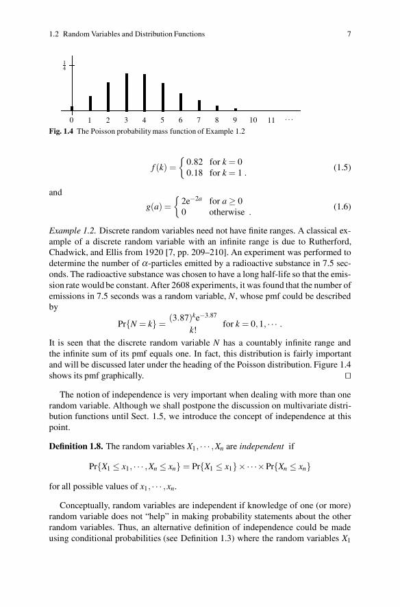
0 1 2 3 4 5 6 7 8 9 10 11 · · ·Fig. 1.4 The Poisson probability mass function of Example 1.2
f (k) ={
0.82 for k = 00.18 for k = 1 .
(1.5)
and
g(a) ={
2e−2a for a ≥ 00 otherwise .
(1.6)
Example 1.2. Discrete random variables need not have finite ranges. A classical ex-ample of a discrete random variable with an infinite range is due to Rutherford,Chadwick, and Ellis from 1920 [7, pp. 209–210]. An experiment was performed todetermine the number of α-particles emitted by a radioactive substance in 7.5 sec-onds. The radioactive substance was chosen to have a long half-life so that the emis-sion rate would be constant. After 2608 experiments, it was found that the number ofemissions in 7.5 seconds was a random variable, N , whose pmf could be describedby
Pr{N = k} =(3.87)ke−3.87
k!for k = 0,1, · · · .
It is seen that the discrete random variable N has a countably infinite range andthe infinite sum of its pmf equals one. In fact, this distribution is fairly importantand will be discussed later under the heading of the Poisson distribution. Figure 1.4shows its pmf graphically. ��
The notion of independence is very important when dealing with more than onerandom variable. Although we shall postpone the discussion on multivariate distri-bution functions until Sect. 1.5, we introduce the concept of independence at thispoint.
Definition 1.8. The random variables X1, · · · ,Xn are independent if
Pr{X1 ≤ x1, · · · ,Xn ≤ xn} = Pr{X1 ≤ x1}× · · ·×Pr{Xn ≤ xn}
for all possible values of x1, · · · ,xn.
Conceptually, random variables are independent if knowledge of one (or more)random variable does not “help” in making probability statements about the otherrandom variables. Thus, an alternative definition of independence could be madeusing conditional probabilities (see Definition 1.3) where the random variables X1
8 1 Basic Probability Review
and X2 are called independent if Pr{X1 ≤ x1|X2 ≤ x2} = Pr{X1 ≤ x1} for all valuesof x1 and x2.
For example, suppose that T is a random variable denoting the length of timeit takes for a barge to travel from a refinery to a terminal 800 miles down river,and R is a random variable equal to 1 if the river condition is smooth when the bargeleaves and 0 if the river condition is not smooth. After collecting data to estimate theprobability laws governing T and R, we would not expect the two random variablesto be independent since knowledge of the river conditions would help in determiningthe length of travel time.
One advantage of independence is that it is easier to obtain the distribution forsums of random variables when they are independent than when they are not inde-pendent. When the random variables are continuous, the pdf of the sum involves anintegral called a convolution.
Property 1.2. Let X1 and X2 be independent continuous random variableswith pdf ’s given by f1(·) and f2(·). Let Y = X1 + X2, and let h(·) be the pdffor Y . The pdf for Y can be written, for all y, as
h(y) =∫ ∞
−∞f1(y− x) f2(x)dx .
Furthermore, if X1 and X2 are both nonnegative random variables, then
h(y) =∫ y
0f1(y− x) f2(x)dx .
Example 1.3. Our electronic equipment is highly sensitive to voltage fluctuations inthe power supply so we have collected data to estimate when these fluctuations oc-cur. After much study, it has been determined that the time between voltage spikes isa random variable with pdf given by (1.6), where the unit of time is hours. Further-more, it has been determined that the random variables describing the time betweentwo successive voltage spikes are independent. We have just turned the equipmenton and would like to know the probability that within the next 30 minutes at leasttwo spikes will occur.
Let X1 denote the time interval from when the equipment is turned on until thefirst voltage spike occurs, and let X2 denote the time interval from when the firstspike occurs until the second occurs. The question of interest is to find Pr{Y ≤ 0.5},where Y = X1 +X2. Let the pdf for Y be denoted by h(·). Property 1.2 yields
h(y) =∫ y
04e−2(y−x)e−2xdx
= 4e−2y∫ y
0dx = 4ye−2y ,
for y ≥ 0. The pdf of Y is now used to answer our question, namely,

1.2 Random Variables and Distribution Functions 9
0 X1 ≈ x y
� �y−x
Fig. 1.5 Time line illustrating the convolution
Pr{Y ≤ 0.5}=∫ 0.5
0h(y)dy =
∫ 0.5
04ye−2ydy = 0.264 .
��
It is also interesting to note that the convolution can be used to give the cumu-lative distribution function if the first pdf in the above property is replaced by theCDF; in other words, for nonnegative random variables we have
H(y) =∫ y
0F1(y− x) f2(x)dx . (1.7)
Applying (1.7) to our voltage fluctuation question yields
Pr{Y ≤ 0.5} ≡ H(0.5) =∫ 0.5
0(1− e−2(0.5−x))2e−2xdx = 0.264 .
We rewrite the convolution of Eq. (1.7) slightly to help in obtaining an intuitiveunderstanding of why the convolution is used for sums. Again, assume that X1 andX2 are independent, nonnegative random variables with pdf’s f1 and f2, then
Pr{X1 +X2 ≤ y} =∫ y
0F2(y− x) f1(x)dx .
The interpretation of f1(x)dx is that it represents the probability that the randomvariable X1 falls in the interval (x,x+dx) or, equivalently, that X1 is approximatelyx. Now consider the time line in Fig. 1.5. For the sum to be less than y, two eventsmust occur: first, X1 must be some value (call it x) that is less than y; second, X2
must be less than the remaining time that is y− x. The probability of the first eventis approximately f1(x)dx, and the probability of the second event is F2(y−x). Sincethe two events are independent, they are multiplied together; and since the value ofx can be any number between 0 and y, the integral is from 0 to y.
• Suggestion: Do Problems 1.3–1.6.

10 1 Basic Probability Review
1.3 Mean and Variance
Many random variables have complicated distribution functions and it is thereforedifficult to obtain an intuitive understanding of the behavior of the random variableby simply knowing the distribution function. Two measures, the mean and variance,are defined to aid in describing the randomness of a random variable. The meanequals the arithmetic average of infinitely many observations of the random vari-able and the variance is an indication of the variability of the random variable. Toillustrate this concept we use the square root of the variance which is called thestandard deviation. In the 19th century, the Russian mathematician P. L. Chebyshevshowed that for any given distribution, at least 75% of the time the observed valueof a random variable will be within two standard deviations of its mean and at least93.75% of the time the observed value will be within four standard deviations ofthe mean. These are general statements, and specific distributions will give muchtighter bounds. (For example, a commonly used distribution is the normal “bellshaped” distribution. With the normal distribution, there is a 95.44% probability ofbeing within two standard deviations of the mean.) Both the mean and variance aredefined in terms of the expected value operator, that we now define.
Definition 1.9. Let h be a function defined on the real numbers and let X be a ran-dom variable. The expected value of h(X) is given, for X discrete, by
E[h(X)] = ∑k
h(k) f (k)
where f is its pmf, and for X continuous, by
E[h(X)] =∫ ∞
−∞h(s) f (s)ds
where f is its pdf.
Example 1.4. A supplier sells eggs by the carton containing 144 eggs. There is asmall probability that some eggs will be broken and he refunds money based onbroken eggs. We let B be a random variable indicating the number of broken eggsper carton with a pmf given by
k f (k)0 0.7791 0.1952 0.0243 0.002
.
A carton sells for $4.00, but a refund of 5 cents is made for each broken egg. Todetermine the expected income per carton, we define the function h as follows
1.3 Mean and Variance 11
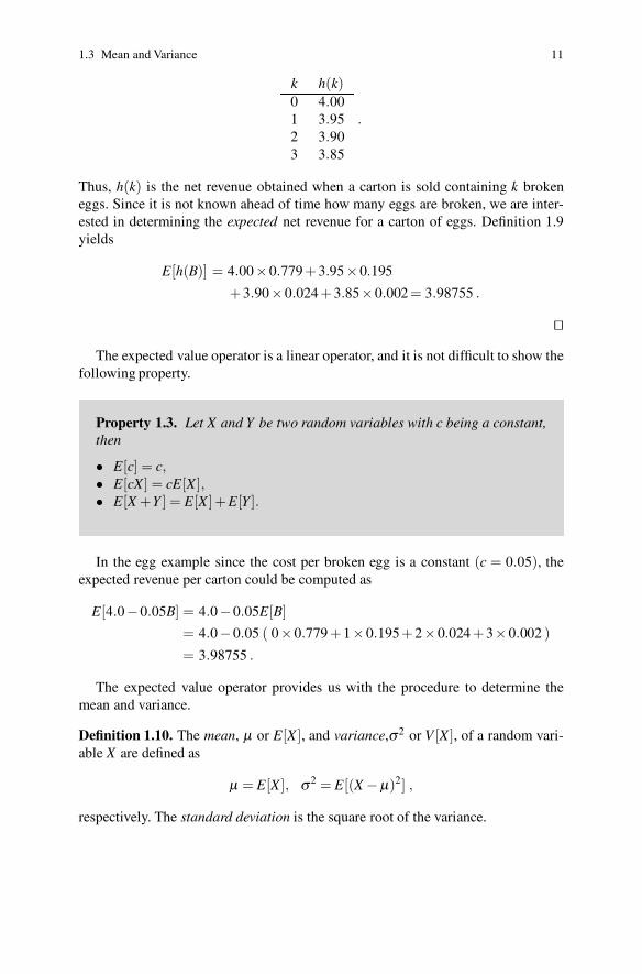
k h(k)0 4.001 3.952 3.903 3.85
.
Thus, h(k) is the net revenue obtained when a carton is sold containing k brokeneggs. Since it is not known ahead of time how many eggs are broken, we are inter-ested in determining the expected net revenue for a carton of eggs. Definition 1.9yields
E[h(B)] = 4.00×0.779 +3.95×0.195
+3.90×0.024 +3.85×0.002 = 3.98755 .
��
The expected value operator is a linear operator, and it is not difficult to show thefollowing property.
Property 1.3. Let X and Y be two random variables with c being a constant,then
• E[c] = c,• E[cX ] = cE[X ],• E[X +Y ] = E[X ]+E[Y ].
In the egg example since the cost per broken egg is a constant (c = 0.05), theexpected revenue per carton could be computed as
E[4.0−0.05B] = 4.0−0.05E[B]= 4.0−0.05 ( 0×0.779 +1×0.195+2×0.024 +3×0.002 )= 3.98755 .
The expected value operator provides us with the procedure to determine themean and variance.
Definition 1.10. The mean, μ or E[X ], and variance,σ2 or V [X ], of a random vari-able X are defined as
μ = E[X ], σ2 = E[(X −μ)2] ,
respectively. The standard deviation is the square root of the variance.
12 1 Basic Probability Review
Property 1.4. The following are often helpful as computational aids:
• V [X ] = σ2 = E[X2]−μ2
• V [cX ] = c2V [X ]• If X ≥ 0, E[X ] =
∫ ∞0 [1−F(s)]ds where F(x) = Pr{X ≤ x}
• If X ≥ 0, then E[X2] = 2∫∞
0 s[1−F(s)]ds where F(x) = Pr{X ≤ x}.
Example 1.5. The mean and variance calculations for a discrete random variable canbe easily illustrated by defining the random variable N to be the number of defectivephones within a randomly chosen box from Example 1.1. In other words, N has thepmf given by
Pr{N = k} =
⎧
⎨
⎩
0.82 for k = 00.15 for k = 10.03 for k = 2 .
The mean and variance is, therefore, given by
E[N] = 0×0.82 +1×0.15+2×0.03
= 0.21,
V [N] = (0−0.21)2×0.82 +(1−0.21)2×0.15 +(2−0.21)2×0.03
= 0.2259 .
Or, an easier calculation for the variance (Property 1.4) is
E[N2] = 02 ×0.82 +12×0.15 +22×0.03
= 0.27
V [N] = 0.27−0.212
= 0.2259 .
��
Example 1.6. The mean and variance calculations for a continuous random variablecan be illustrated with the random variable T whose pdf was given by Eq. 1.6. Themean and variance is therefore given by
E[T ] =∫ ∞
02se−2sds = 0.5 ,
V [T ] =∫ ∞
02(s−0.5)2e−2sds = 0.25 .
Or, an easier calculation for the variance (Property 1.4) is
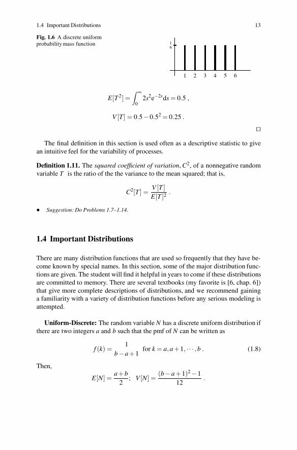
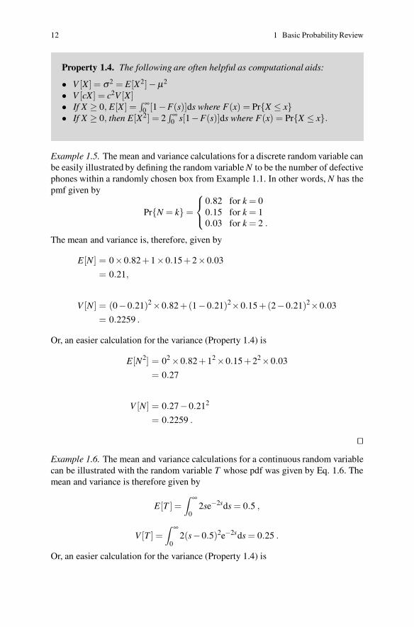
1.4 Important Distributions 13
Fig. 1.6 A discrete uniformprobability mass function 1
6
1 2 3 4 5 6
E[T 2] =∫ ∞
02s2e−2sds = 0.5 ,
V [T ] = 0.5−0.52 = 0.25 .
��
The final definition in this section is used often as a descriptive statistic to givean intuitive feel for the variability of processes.
Definition 1.11. The squared coefficient of variation, C2, of a nonnegative randomvariable T is the ratio of the the variance to the mean squared; that is,
C2[T ] =V [T ]E[T ]2
.
• Suggestion: Do Problems 1.7–1.14.
1.4 Important Distributions
There are many distribution functions that are used so frequently that they have be-come known by special names. In this section, some of the major distribution func-tions are given. The student will find it helpful in years to come if these distributionsare committed to memory. There are several textbooks (my favorite is [6, chap. 6])that give more complete descriptions of distributions, and we recommend gaininga familiarity with a variety of distribution functions before any serious modeling isattempted.
Uniform-Discrete: The random variable N has a discrete uniform distribution ifthere are two integers a and b such that the pmf of N can be written as
f (k) =1
b−a +1for k = a,a +1, · · · ,b . (1.8)
Then,
E[N] =a +b
2; V [N] =
(b−a +1)2−112
.
14 1 Basic Probability Review
12
0 1 2 3 4
p = 13
12
0 1 2 3 4
p = 12
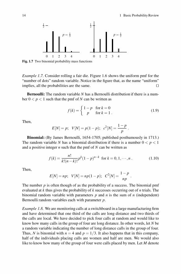
Fig. 1.7 Two binomial probability mass functions
Example 1.7. Consider rolling a fair die. Figure 1.6 shows the uniform pmf for the“number of dots” random variable. Notice in the figure that, as the name “uniform”implies, all the probabilities are the same. ��
Bernoulli: The random variable N has a Bernoulli distribution if there is a num-ber 0 < p < 1 such that the pmf of N can be written as
f (k) ={
1− p for k = 0p for k = 1 .
(1.9)
Then,
E[N] = p; V [N] = p(1− p); c2[N] =1− p
p.
Binomial: (By James Bernoulli, 1654-1705; published posthumously in 1713.)The random variable N has a binomial distribution if there is a number 0 < p < 1and a positive integer n such that the pmf of N can be written as
f (k) =n!
k!(n− k)!pk(1− p)n−k for k = 0,1, · · · ,n . (1.10)
Then,
E[N] = np; V [N] = np(1− p); C2[N] =1− p
np.
The number p is often though of as the probability of a success. The binomial pmfevaluated at k thus gives the probability of k successes occurring out of n trials. Thebinomial random variable with parameters p and n is the sum of n (independent)Bernoulli random variables each with parameter p.
Example 1.8. We are monitoring calls at a switchboard in a large manufacturing firmand have determined that one third of the calls are long distance and two thirds ofthe calls are local. We have decided to pick four calls at random and would like toknow how many calls in the group of four are long distance. In other words, let N bea random variable indicating the number of long distance calls in the group of four.Thus, N is binomial with n = 4 and p = 1/3. It also happens that in this company,half of the individuals placing calls are women and half are men. We would alsolike to know how many of the group of four were calls placed by men. Let M denote
1.4 Important Distributions 15
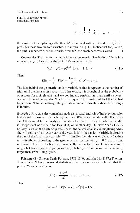
Fig. 1.8 A geometric proba-bility mass function
12
0 1 2 3 4 5 6 7 · · ·
the number of men placing calls; thus, M is binomial with n = 4 and p = 1/2. Thepmf’s for these two random variables are shown in Fig. 1.7. Notice that for p = 0.5,the pmf is symmetric, and as p varies from 0.5, the graph becomes skewed. ��
Geometric: The random variable N has a geometric distribution if there is anumber 0 < p < 1 such that the pmf of N can be written as
f (k) = p(1− p)k−1 for k = 1,2, · · · . (1.11)
Then,
E[N] =1p
; V [N] =1− p
p2 ; C2[N] = 1− p.
The idea behind the geometric random variable is that it represents the number oftrials until the first success occurs. In other words, p is thought of as the probabilityof success for a single trial, and we continually perform the trials until a successoccurs. The random variable N is then set equal to the number of trial that we hadto perform. Note that although the geometric random variable is discrete, its rangeis infinite.
Example 1.9. A car saleswoman has made a statistical analysis of her previous saleshistory and determined that each day there is a 50% chance that she will sell a luxurycar. After careful further analysis, it is also clear that a luxury car sale on one dayis independent of the sale (or lack of it) on another day. On New Year’s Day (aholiday in which the dealership was closed) the saleswoman is contemplating whenshe will sell her first luxury car of the year. If N is the random variable indicatingthe day of the first luxury car sale (N = 1 implies the sale was on January 2), thenN is distributed according to the geometric distribution with p = 0.5, and its pmfis shown in Fig. 1.8. Notice that theoretically the random variable has an infiniterange, but for all practical purposes the probability of the random variable beinglarger than seven is negligible. ��
Poisson: (By Simeon Denis Poisson, 1781-1840; published in 1837.) The ran-dom variable N has a Poisson distribution if there is a number λ > 0 such that thepmf of N can be written as
f (k) =λ ke−λ
k!for k = 0,1, · · · . (1.12)
Then,E[N] = λ ; V [N] = λ ; C2[N] = 1/λ .
16 1 Basic Probability Review
The Poisson distribution is the most important discrete distribution in stochasticmodeling. It arises in many different circumstances. One use is as an approximationto the binomial distribution. For n large and p small, the binomial is approximatedby the Poisson by setting λ = np. For example, suppose we have a box of 144eggs and there is a 1% probability that any one egg will break. Assuming that thebreakage of eggs is independent of other eggs breaking, the probability that exactly 3eggs will be broken out of the 144 can be determined using the binomial distributionwith n = 144, p = 0.01, and k = 3; thus
144!141!3!
(0.01)3(0.99)141 = 0.1181 ,
or by the Poisson approximation with λ = 1.44 that yields
(1.44)3e−1.44
3!= 0.1179 .
In 1898, L. V. Bortkiewicz [7, p. 206] reported that the number of deaths dueto horse-kicks in the Prussian army was a Poisson random variable. Although thisseems like a silly example, it is very instructive. The reason that the Poisson distri-bution holds in this case is due to the binomial approximation feature of the Poisson.Consider the situation: there would be a small chance of death by horse-kick for anyone person (i.e., p small) but a large number of individuals in the army (i.e., n large).There are many analogous situations in modeling that deal with large populationsand a small chance of occurrence for any one individual within the population. Inparticular, arrival processes (like arrivals to a bus station in a large city) can often beviewed in this fashion and thus described by a Poisson distribution. Another com-mon use of the Poisson distribution is in population studies. The population size ofa randomly growing organism often can be described by a Poisson random variable.W. S. Gosset, using the pseudonym of Student, showed in 1907 that the numberof yeast cells in 400 squares of haemocytometer followed a Poisson distribution.Radioactive emissions are also Poisson as indicated in Example 1.2. (Fig. 1.4 alsoshows the Poisson pmf.)
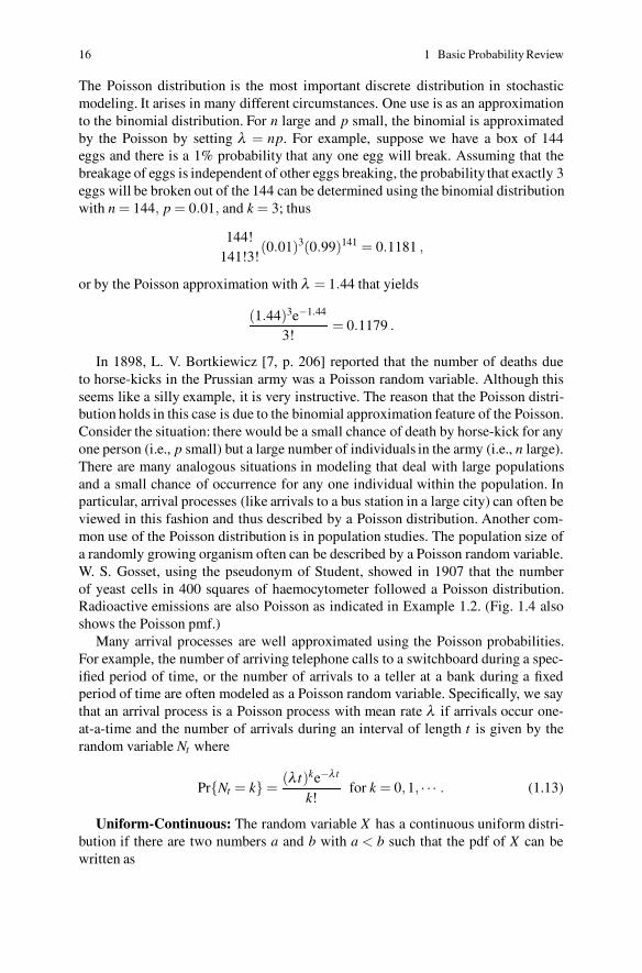
Many arrival processes are well approximated using the Poisson probabilities.For example, the number of arriving telephone calls to a switchboard during a spec-ified period of time, or the number of arrivals to a teller at a bank during a fixedperiod of time are often modeled as a Poisson random variable. Specifically, we saythat an arrival process is a Poisson process with mean rate λ if arrivals occur one-at-a-time and the number of arrivals during an interval of length t is given by therandom variable Nt where
Pr{Nt = k} =(λ t)ke−λ t
k!for k = 0,1, · · · . (1.13)
Uniform-Continuous: The random variable X has a continuous uniform distri-bution if there are two numbers a and b with a < b such that the pdf of X can bewritten as

1.4 Important Distributions 17
12
0 1 2 3
�����1.0
0 1 2 3
Fig. 1.9 The probability density function and cumulative distribution function for a continuousuniform distribution between 1 and 3
f (s) ={ 1
b−a for a ≤ s ≤ b0 otherwise .
(1.14)
Then its cumulative probability distribution is given by
F(s) =
⎧
⎨
⎩
0 for s < as−ab−a for a ≤ s < b1 for s ≥ b ,
and
E[X ] =a +b
2; V [X ] =
(b−a)2
12; C2[X ] =
(b−a)2
3(a +b)2 .
The graphs for the pdf and CDF of the continuous uniform random variables arethe simplest of the continuous distributions. As shown in Fig. 1.9, the pdf is a rect-angle and the CDF is a “ramp” function.
Exponential: The random variable X has an exponential distribution if there is anumber λ > 0 such that the pdf of X can be written as
f (s) ={
λ e−λ s for s ≥ 00 otherwise .
(1.15)
Then its cumulative probability distribution is given by
F(s) ={
0 for s < 0,
1− e−λ s for s ≥ 0;
and
E[X ] =1λ
; V [X ] =1
λ 2 ; C2[X ] = 1 .
The exponential distribution is an extremely common distribution in probabilis-tic modeling. One very important feature is that the exponential distribution is theonly continuous distribution that contains no memory. Specifically, an exponentialrandom variable X is said to be memoryless if
Pr{X > t + s|X > t}= Pr{X > s} . (1.16)
18 1 Basic Probability Review
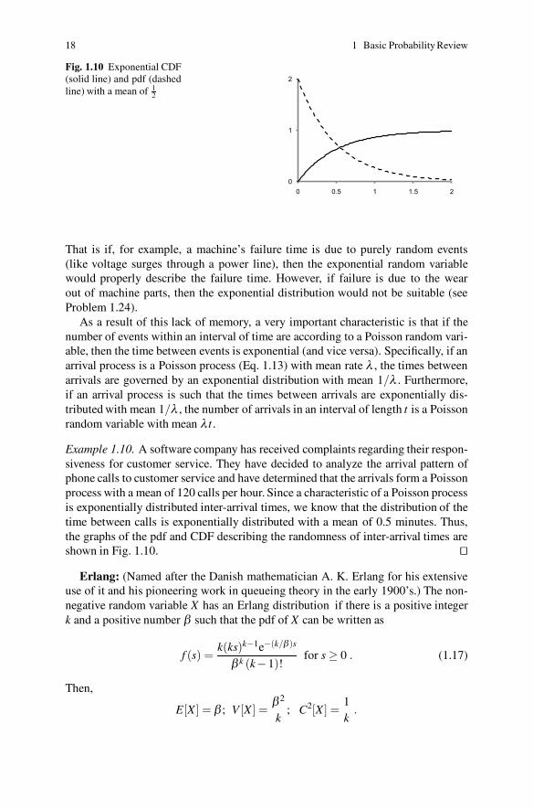
Fig. 1.10 Exponential CDF(solid line) and pdf (dashedline) with a mean of 1
2
0
1
2
0 0.5 1 1.5 2
That is if, for example, a machine’s failure time is due to purely random events(like voltage surges through a power line), then the exponential random variablewould properly describe the failure time. However, if failure is due to the wearout of machine parts, then the exponential distribution would not be suitable (seeProblem 1.24).
As a result of this lack of memory, a very important characteristic is that if thenumber of events within an interval of time are according to a Poisson random vari-able, then the time between events is exponential (and vice versa). Specifically, if anarrival process is a Poisson process (Eq. 1.13) with mean rate λ , the times betweenarrivals are governed by an exponential distribution with mean 1/λ . Furthermore,if an arrival process is such that the times between arrivals are exponentially dis-tributed with mean 1/λ , the number of arrivals in an interval of length t is a Poissonrandom variable with mean λ t .
Example 1.10. A software company has received complaints regarding their respon-siveness for customer service. They have decided to analyze the arrival pattern ofphone calls to customer service and have determined that the arrivals form a Poissonprocess with a mean of 120 calls per hour. Since a characteristic of a Poisson processis exponentially distributed inter-arrival times, we know that the distribution of thetime between calls is exponentially distributed with a mean of 0.5 minutes. Thus,the graphs of the pdf and CDF describing the randomness of inter-arrival times areshown in Fig. 1.10. ��
Erlang: (Named after the Danish mathematician A. K. Erlang for his extensiveuse of it and his pioneering work in queueing theory in the early 1900’s.) The non-negative random variable X has an Erlang distribution if there is a positive integerk and a positive number β such that the pdf of X can be written as
f (s) =k(ks)k−1e−(k/β )s
β k (k−1)!for s ≥ 0 . (1.17)
Then,
E[X ] = β ; V [X ] =β 2
k; C2[X ] =
1k
.
1.4 Important Distributions 19
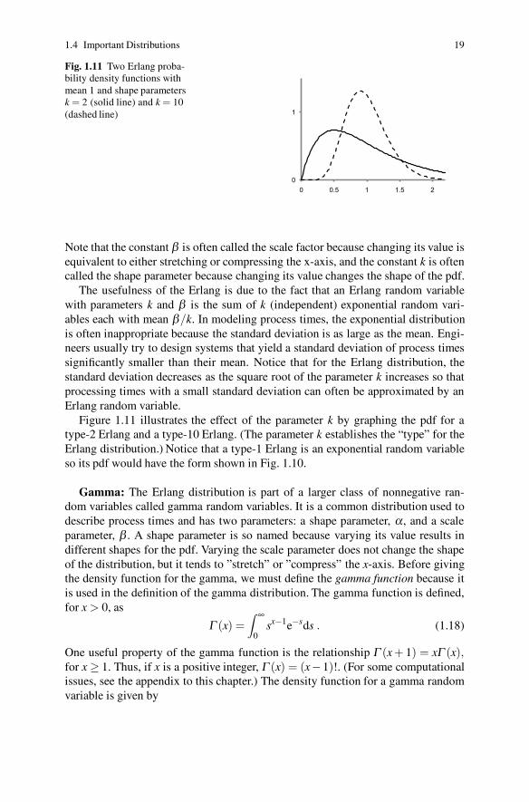
Fig. 1.11 Two Erlang proba-bility density functions withmean 1 and shape parametersk = 2 (solid line) and k = 10(dashed line)
0
1
0 0.5 1 1.5 2
Note that the constant β is often called the scale factor because changing its value isequivalent to either stretching or compressing the x-axis, and the constant k is oftencalled the shape parameter because changing its value changes the shape of the pdf.
The usefulness of the Erlang is due to the fact that an Erlang random variablewith parameters k and β is the sum of k (independent) exponential random vari-ables each with mean β/k. In modeling process times, the exponential distributionis often inappropriate because the standard deviation is as large as the mean. Engi-neers usually try to design systems that yield a standard deviation of process timessignificantly smaller than their mean. Notice that for the Erlang distribution, thestandard deviation decreases as the square root of the parameter k increases so thatprocessing times with a small standard deviation can often be approximated by anErlang random variable.
Figure 1.11 illustrates the effect of the parameter k by graphing the pdf for atype-2 Erlang and a type-10 Erlang. (The parameter k establishes the “type” for theErlang distribution.) Notice that a type-1 Erlang is an exponential random variableso its pdf would have the form shown in Fig. 1.10.
Gamma: The Erlang distribution is part of a larger class of nonnegative ran-dom variables called gamma random variables. It is a common distribution used todescribe process times and has two parameters: a shape parameter, α, and a scaleparameter, β . A shape parameter is so named because varying its value results indifferent shapes for the pdf. Varying the scale parameter does not change the shapeof the distribution, but it tends to ”stretch” or ”compress” the x-axis. Before givingthe density function for the gamma, we must define the gamma function because itis used in the definition of the gamma distribution. The gamma function is defined,for x > 0, as
Γ (x) =∫ ∞
0sx−1e−sds . (1.18)
One useful property of the gamma function is the relationship Γ (x + 1) = xΓ (x),for x ≥ 1. Thus, if x is a positive integer, Γ (x) = (x−1)!. (For some computationalissues, see the appendix to this chapter.) The density function for a gamma randomvariable is given by

20 1 Basic Probability Review
Fig. 1.12 Two Weibull prob-ability density functions withmean 1 and shape parametersα = 0.5 (solid line) and α = 2(dashed line)
0
1
0 0.5 1 1.5 2
f (s) =sα−1e−s/β
β k Γ (α −1)for s ≥ 0 . (1.19)
Then,
E[X ] = β α; V [X ] = β 2α; C2[X ] =1α
.
Notice that if it is desired to determine the shape and scale parameters for a gammadistribution with a known mean and variance, the inverse relationships are
α =E[X ]2
V [X ]and β =
E[X ]α
.
Weibull: In 1939, W. Weibull [2, p. 73] developed a distribution for describingthe breaking strength of various materials. Since that time, many statisticians haveshown that the Weibull distribution can often be used to describe failure times formany different types of systems. The Weibull distribution has two parameters: ascale parameter, β , and a shape parameter, α. Its cumulative distribution function isgiven by
F(s) ={
0 for s < 01− e−(s/β )α
for s ≥ 0 .
Both scale and shape parameters can be any positive number. As with the gammadistribution, the shape parameter determines the general shape of the pdf (seeFig. 1.12) and the scale parameter either expands or contracts the pdf. The mo-ments of the Weibull are a little difficult to express because they involve the gammafunction (1.18). Specifically, the moments for the Weibull distribution are
E[X ] = βΓ (1 +1α
); E[X2] = β 2Γ (1 +2α
); E[X3] = β 3Γ (1 +3α
) . (1.20)
It is more difficult to determine the shape and scale parameters for a Weibull dis-tribution with a known mean and variance, than it is for the gamma distributionbecause the gamma function must be evaluated to determine the moments of aWeibull. Some computational issues for obtaining the shape and scale parametersof a Weibull are discussed in the appendix to this chapter.

1.4 Important Distributions 21
Fig. 1.13 Standard normalpdf (solid line) and CDF(dashed line)
0
1
-3 -2 -1 0 1 2 3
When the shape parameter is greater than 1, the shape of the Weibull pdf is uni-modal similar to the Erlang with its type parameter greater than 1. When the shapeparameter equals 1, the Weibull pdf is an exponential pdf. When the shape parameteris less than 1, the pdf is similar to the exponential except that the graph is asymp-totic to the y-axis instead of hitting the y-axis. Figure 1.12 provides an illustrationof the effect that the shape parameter has on the Weibull distribution. Because themean values were held constant for the two pdf’s shown in the figure, the value forβ varied. The pdf plotted with a solid line in the figure has β = 0.5 that, togetherwith α = 0.5, yields a mean of 1 and a standard deviation of 2.236; the dashed lineis pdf that has β = 1.128 that, together with α = 2, yields a mean of 1 and a standarddeviation 0.523.
Normal: (Discovered by A. de Moivre, 1667-1754, but usually attributed to KarlGauss, 1777-1855.) The random variable X has a normal distribution if there aretwo numbers μ and σ with σ > 0 such that the pdf of X can be written as
f (s) =1
σ√
2πe−(s−μ)2/(2σ 2) for −∞ < s < ∞ . (1.21)
Then,
E[X ] = μ; V [X ] = σ2; C2[X ] =σ2
μ2 .
The normal distribution is the most common distribution recognized by mostpeople by its “bell shaped” curve. Its pdf and CDF are shown below in Fig. 1.13 fora normally distributed random variable with mean zero and standard deviation one.
Although the normal distribution is not widely used in stochastic modeling, itis, without question, the most important distribution in statistics. The normal dis-tribution can be used to approximate both the binomial and Poisson distributions.A common rule-of-thumb is to approximate the binomial whenever n (the numberof trials) is larger than 30. If np < 5, then use the Poisson for the approximationwith λ = np. If np ≥ 5, then use the normal for the approximation with μ = np andσ2 = np(1− p). Furthermore, the normal can be used to approximate the Poissonwhenever λ > 30. When using a continuous distribution (like the normal) to approx-
22 1 Basic Probability Review
imate a discrete distribution (like the Poisson or binomial), the interval between thediscrete values is usually split halfway. For example, if we desire to approximatethe probability that a Poisson random variable will take on the values 29, 30, or31 with a continuous distribution, then we would determine the probability that thecontinuous random variable is between 28.5 and 31.5.
Example 1.11. The software company mentioned in the previous example has de-termined that the arrival process is Poisson with a mean arrival rate of 120 per hour.The company would like to know the probability that in any one hour 140 or morecalls arrive. To determine that probability, let N be a Poisson random variable withλ = 120, let X be a random variable with μ = σ2 = 120 and let Z be a standardnormal random variable (i.e., Z is normal with mean 0 and variance 1). The abovequestion is answered as follows:
Pr{N ≥ 140} ≈ Pr{X > 139.5}= Pr{Z > (139.5−120)/10.95}= Pr{Z > 1.78}= 1−0.9625 = 0.0375 .
��
The importance of the normal distribution is due to its property that samplemeans from almost any practical distribution will limit to the normal; this prop-erty is called the Central Limit Theorem. We state this property now even though itneeds the concept of statistical independence that is not yet defined. However, be-cause the idea should be somewhat intuitive, we state the property at this point sinceit is so central to the use of the normal distribution.
Property 1.5. Central Limit Theorem. Let {X1,X2, · · · ,Xn } be a sequenceof n independent random variables each having the same distribution withmean μ and (finite) variance σ2, and define
X =X1 +X2 + · · ·+Xn
n.
Then, the distribution of the random variable Z defined by
Z =X −μσ/
√n
approaches a normal distribution with zero mean and standard deviation ofone as n gets large.
Skewness: Before moving to the discussion of more than one random variable,we mention an additional descriptor of distributions. The first moment gives thecentral tendency for random variables, and the second moment is used to measure
1.5 Multivariate Distributions 23
variability. The third moment, that was not discussed previously, is useful as a mea-sure of skewness (i.e., non-symmetry). Specifically, the coefficient of skewness, ν ,for a random variable T with mean μ and standard deviation σ is defined by
ν =E[(T −μ)3]
σ3 , (1.22)
and the relation to the other moments is
E[(T −μ)3] = E[T 3]−3μE[T 2]+2μ3 .
A symmetric distribution has ν = 0; if the mean is to the left of the mode, ν < 0and the left-hand side of the distribution will have the longer tail; if the mean is tothe right of the mode, ν > 0 and the right-hand side of the distribution will havethe longer tail. For example, ν = 0 for the normal distribution, ν = 2 for the ex-ponential distribution, ν = 2/
√k for a type-k Erlang distribution, and for a gamma
distribution, we have ν = 2/√
α . The Weibull pdf’s shown in Fig. 1.12 have skew-ness coefficients of 3.9 and 0.63, respectively, for the solid line figure and dashedline graphs. Thus, the value of ν can help complete the intuitive understanding of aparticular distribution.
• Suggestion: Do Problems 1.15–1.19.
1.5 Multivariate Distributions
The analysis of physical phenomena usually involves many distinct random vari-ables. In this section we discuss the concepts involved when two random variablesare defined. The extension to more than two is left to the imagination of the readerand the numerous textbooks that have been written on the subject.
Definition 1.12. The function F is called the joint cumulative distribution functionfor X1 and X2 if
F(a,b) = Pr{X1 ≤ a,X2 ≤ b}for a and b any two real numbers.
In a probability statement as in the right-hand-side of the above equation, thecomma means intersection of events and is read as “The probability that X1 is lessthan or equal to a and X2 is less than or equal to b”. The initial understanding ofjoint probabilities is easiest with discrete random variables.
Definition 1.13. The function f is a joint pmf for the discrete random variables X1
and X2 iff (a,b) = Pr{X1 = a,X2 = b}
for each (a,b) in the range of (X1,X2).
24 1 Basic Probability Review
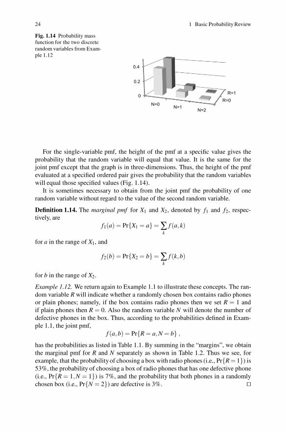
Fig. 1.14 Probability massfunction for the two discreterandom variables from Exam-ple 1.12
R=0R=10
0.2
0.4
N=0 N=1 N=2
For the single-variable pmf, the height of the pmf at a specific value gives theprobability that the random variable will equal that value. It is the same for thejoint pmf except that the graph is in three-dimensions. Thus, the height of the pmfevaluated at a specified ordered pair gives the probability that the random variableswill equal those specified values (Fig. 1.14).
It is sometimes necessary to obtain from the joint pmf the probability of onerandom variable without regard to the value of the second random variable.
Definition 1.14. The marginal pmf for X1 and X2, denoted by f1 and f2, respec-tively, are
f1(a) = Pr{X1 = a}= ∑k
f (a,k)
for a in the range of X1, and
f2(b) = Pr{X2 = b}= ∑k
f (k,b)
for b in the range of X2.
Example 1.12. We return again to Example 1.1 to illustrate these concepts. The ran-dom variable R will indicate whether a randomly chosen box contains radio phonesor plain phones; namely, if the box contains radio phones then we set R = 1 andif plain phones then R = 0. Also the random variable N will denote the number ofdefective phones in the box. Thus, according to the probabilities defined in Exam-ple 1.1, the joint pmf,
f (a,b) = Pr{R = a,N = b} ,
has the probabilities as listed in Table 1.1. By summing in the “margins”, we obtainthe marginal pmf for R and N separately as shown in Table 1.2. Thus we see, forexample, that the probability of choosing a box with radio phones (i.e., Pr{R = 1}) is53%, the probability of choosing a box of radio phones that has one defective phone(i.e., Pr{R = 1,N = 1}) is 7%, and the probability that both phones in a randomlychosen box (i.e., Pr{N = 2}) are defective is 3%. ��
1.5 Multivariate Distributions 25
Table 1.1 Joint probability mass function of Example 1.12
N = 0 N = 1 N = 2R = 0 0.37 0.08 0.02R = 1 0.45 0.07 0.01
Table 1.2 Marginal probability mass functions of Example 1.12
N = 0 N = 1 N = 2 f1(·)R = 0 0.37 0.08 0.02 0.47R = 1 0.45 0.07 0.01 0.53f2(·) 0.82 0.15 0.03
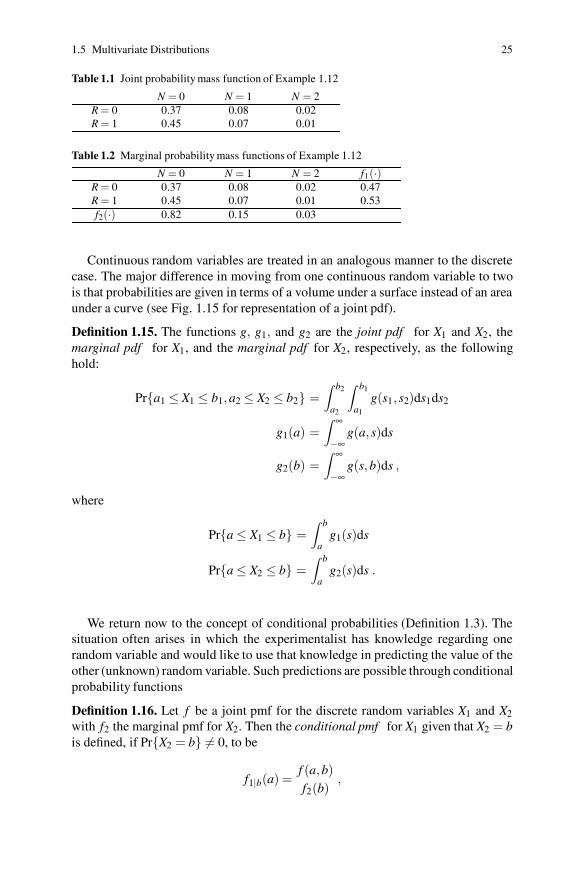
Continuous random variables are treated in an analogous manner to the discretecase. The major difference in moving from one continuous random variable to twois that probabilities are given in terms of a volume under a surface instead of an areaunder a curve (see Fig. 1.15 for representation of a joint pdf).
Definition 1.15. The functions g, g1, and g2 are the joint pdf for X1 and X2, themarginal pdf for X1, and the marginal pdf for X2, respectively, as the followinghold:
Pr{a1 ≤ X1 ≤ b1,a2 ≤ X2 ≤ b2} =∫ b2
a2
∫ b1
a1
g(s1, s2)ds1ds2
g1(a) =∫ ∞
−∞g(a, s)ds
g2(b) =∫ ∞
−∞g(s,b)ds ,
where
Pr{a ≤ X1 ≤ b} =∫ b
ag1(s)ds
Pr{a ≤ X2 ≤ b} =∫ b
ag2(s)ds .
We return now to the concept of conditional probabilities (Definition 1.3). Thesituation often arises in which the experimentalist has knowledge regarding onerandom variable and would like to use that knowledge in predicting the value of theother (unknown) random variable. Such predictions are possible through conditionalprobability functions
Definition 1.16. Let f be a joint pmf for the discrete random variables X1 and X2
with f2 the marginal pmf for X2. Then the conditional pmf for X1 given that X2 = bis defined, if Pr{X2 = b} �= 0, to be
f1|b(a) =f (a,b)f2(b)
,
26 1 Basic Probability Review
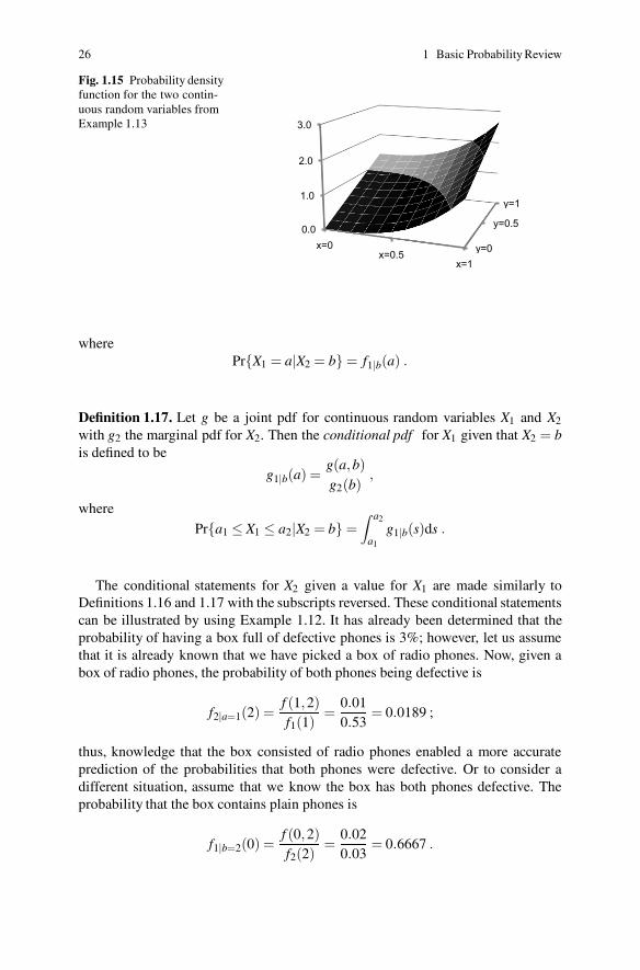
Fig. 1.15 Probability densityfunction for the two contin-uous random variables fromExample 1.13
y=0
y=0.5
y=1
0.0
1.0
2.0
3.0
x=0x=0.5
x=1
wherePr{X1 = a|X2 = b} = f1|b(a) .
Definition 1.17. Let g be a joint pdf for continuous random variables X1 and X2
with g2 the marginal pdf for X2. Then the conditional pdf for X1 given that X2 = bis defined to be
g1|b(a) =g(a,b)g2(b)
,
where
Pr{a1 ≤ X1 ≤ a2|X2 = b} =∫ a2
a1
g1|b(s)ds .
The conditional statements for X2 given a value for X1 are made similarly toDefinitions 1.16 and 1.17 with the subscripts reversed. These conditional statementscan be illustrated by using Example 1.12. It has already been determined that theprobability of having a box full of defective phones is 3%; however, let us assumethat it is already known that we have picked a box of radio phones. Now, given abox of radio phones, the probability of both phones being defective is
f2|a=1(2) =f (1,2)f1(1)
=0.010.53
= 0.0189 ;
thus, knowledge that the box consisted of radio phones enabled a more accurateprediction of the probabilities that both phones were defective. Or to consider adifferent situation, assume that we know the box has both phones defective. Theprobability that the box contains plain phones is
f1|b=2(0) =f (0,2)f2(2)
=0.020.03
= 0.6667 .
1.5 Multivariate Distributions 27
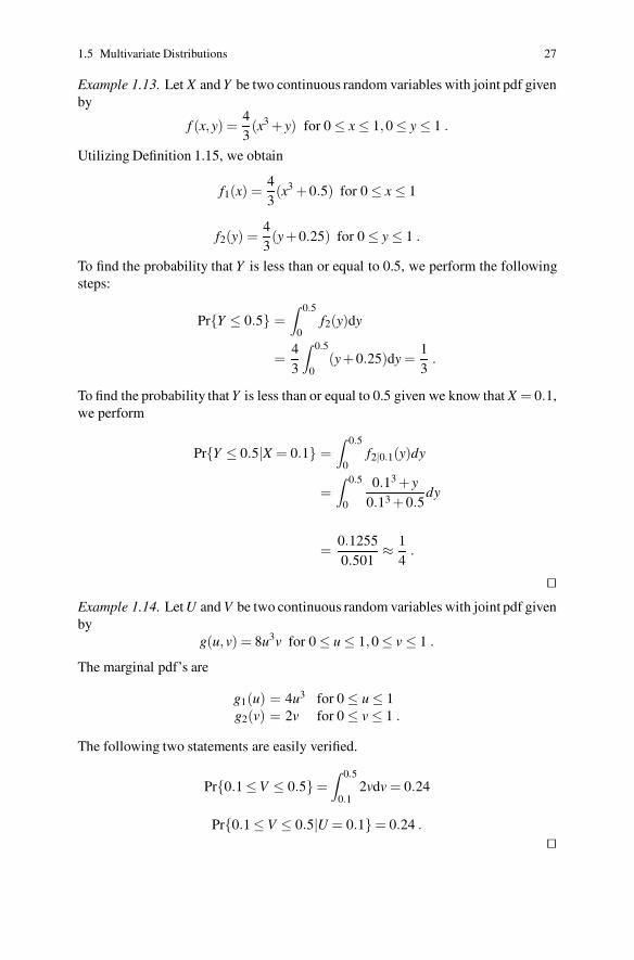
Example 1.13. Let X and Y be two continuous random variables with joint pdf givenby
f (x,y) =43(x3 + y) for 0 ≤ x ≤ 1,0 ≤ y ≤ 1 .
Utilizing Definition 1.15, we obtain
f1(x) =43(x3 +0.5) for 0 ≤ x ≤ 1
f2(y) =43(y+0.25) for 0 ≤ y ≤ 1 .
To find the probability that Y is less than or equal to 0.5, we perform the followingsteps:
Pr{Y ≤ 0.5} =∫ 0.5
0f2(y)dy
=43
∫ 0.5
0(y+0.25)dy =
13
.
To find the probability that Y is less than or equal to 0.5 given we know that X = 0.1,we perform
Pr{Y ≤ 0.5|X = 0.1} =∫ 0.5
0f2|0.1(y)dy
=∫ 0.5
0
0.13 + y0.13 +0.5
dy
=0.12550.501
≈ 14
.
��Example 1.14. Let U and V be two continuous random variables with joint pdf givenby
g(u,v) = 8u3v for 0 ≤ u ≤ 1,0 ≤ v ≤ 1 .
The marginal pdf’s are
g1(u) = 4u3 for 0 ≤ u ≤ 1g2(v) = 2v for 0 ≤ v ≤ 1 .
The following two statements are easily verified.
Pr{0.1 ≤V ≤ 0.5}=∫ 0.5
0.12vdv = 0.24
Pr{0.1 ≤ V ≤ 0.5|U = 0.1}= 0.24 .
��

28 1 Basic Probability Review
The above example illustrates independence. Notice in the example that knowl-edge of the value of U did not change the probabilities regarding the probabilitystatement of V .
Definition 1.18. Let f be the joint probability distribution (pmf if discrete and pdfif continuous) of two random variables X1 and X2. Furthermore, let f1 and f2 be themarginals for X1 and X2, respectively. If
f (a,b) = f1(a) f2(b)
for all a and b, then X1 and X2 are called independent.
Independent random variables are much easier to work with because of theirseparability. However, in the use of the above definition, it is important to test theproperty for all values of a and b. It would be easy to make a mistake by stoppingafter the equality was shown to hold for only one particular pair of a,b values. Onceindependence has been shown, the following property is very useful.
Property 1.6. Let X1 and X2 be independent random variables. Then
E[X1X2] = E[X1]E[X2]
andV [X1 +X2] = V [X1]+V [X2] .
Example 1.15. Consider again the random variables R and N defined in Example1.12. We see from the marginal pmf’s given in that example that E[R] = 0.53 andE[N] = 0.21. We also have
E[R ·N] = 0×0×0.37 +0×1×0.08 +0×2×0.02
+1×0×0.45 +1×1×0.07 +1×2×0.01 = 0.09 .
Thus, it is possible to say that the random variables R and N are not independentsince 0.53× 0.21 �= 0.09. If, however, the expected value of the product of tworandom variables equals the product of the two individual expected values, the claimof independence is not proven. ��
We close this section by giving two final measures that are used to express therelationship between two dependent random variables. The first measure is calledthe covariance and the second measure is called the correlation coefficient.
Definition 1.19. The covariance of two random variables, X1 and X2, is defined by
cov(X1,X2) = E[ (X1 −E[X1])(X2 −E[X2]) ] .
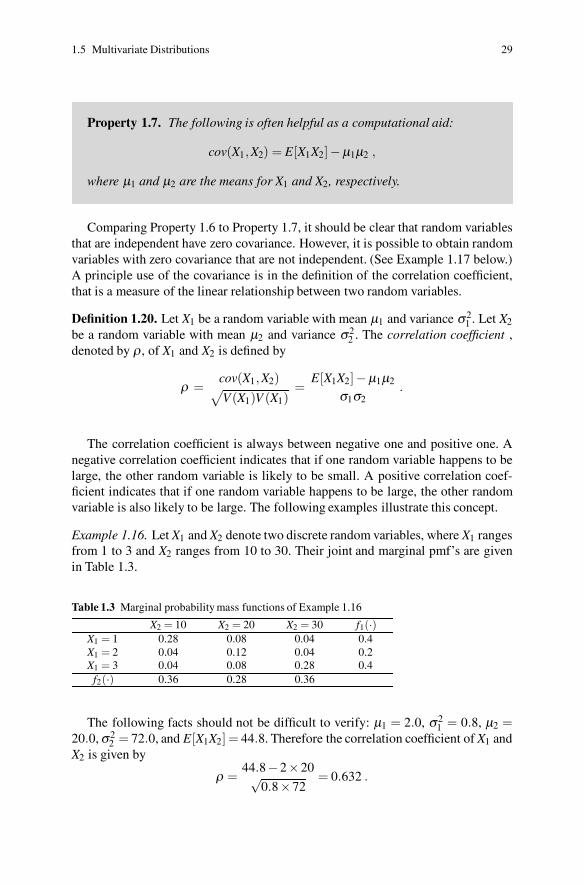
1.5 Multivariate Distributions 29
Property 1.7. The following is often helpful as a computational aid:
cov(X1,X2) = E[X1X2]−μ1μ2 ,
where μ1 and μ2 are the means for X1 and X2, respectively.
Comparing Property 1.6 to Property 1.7, it should be clear that random variablesthat are independent have zero covariance. However, it is possible to obtain randomvariables with zero covariance that are not independent. (See Example 1.17 below.)A principle use of the covariance is in the definition of the correlation coefficient,that is a measure of the linear relationship between two random variables.
Definition 1.20. Let X1 be a random variable with mean μ1 and variance σ21 . Let X2
be a random variable with mean μ2 and variance σ22 . The correlation coefficient ,
denoted by ρ , of X1 and X2 is defined by
ρ =cov(X1,X2)√
V(X1)V (X1)=
E[X1X2]−μ1μ2
σ1σ2.
The correlation coefficient is always between negative one and positive one. Anegative correlation coefficient indicates that if one random variable happens to belarge, the other random variable is likely to be small. A positive correlation coef-ficient indicates that if one random variable happens to be large, the other randomvariable is also likely to be large. The following examples illustrate this concept.
Example 1.16. Let X1 and X2 denote two discrete random variables, where X1 rangesfrom 1 to 3 and X2 ranges from 10 to 30. Their joint and marginal pmf’s are givenin Table 1.3.
Table 1.3 Marginal probability mass functions of Example 1.16
X2 = 10 X2 = 20 X2 = 30 f1(·)X1 = 1 0.28 0.08 0.04 0.4X1 = 2 0.04 0.12 0.04 0.2X1 = 3 0.04 0.08 0.28 0.4
f2(·) 0.36 0.28 0.36
The following facts should not be difficult to verify: μ1 = 2.0, σ21 = 0.8, μ2 =
20.0, σ22 = 72.0, and E[X1X2] = 44.8. Therefore the correlation coefficient of X1 and
X2 is given by
ρ =44.8−2×20√
0.8×72= 0.632 .

30 1 Basic Probability Review
Fig. 1.16 Graphical rep-resentation for conditionalprobabilities of X2 given X1from Example 1.16, wherethe correlation coefficient is0.632 10
20
30
1 2 3
�
�
�
�
�
�
�
�
�
The conditional probabilities will help verify the intuitive concept of a positive cor-relation coefficient. Figure 1.16 contains a graph illustrating the conditional prob-abilities of X2 given various values of X1; the area of each circle in the figure isproportional to the conditional probability. Thus, the figure gives a visual represen-tation that as X1 increases, it is likely (but not necessary) that X2 will increase. Forexample, the top right-hand circle represents Pr{X2 = 30|X1 = 3} = 0.7, and themiddle right-hand circle represents Pr{X2 = 20|X1 = 3} = 0.2.
As a final example, we switch the top and middle right-hand circles in Fig. 1.16so that the appearance is not so clearly linear. (That is, let Pr{X1 = 3,X2 = 20} =0.28, Pr{X1 = 3,X2 = 30} = 0.08, and all other probabilities the same.) With thischange, μ1 and σ2
1 remain unchanged, μ2 = 18, σ22 = 48.0, cov(X1,X2) = 2.8 and
the correlation coefficient is ρ = 0.452. Thus, as the linear relationship between X1
and X2 weakens, the value of ρ becomes smaller. ��
If the random variables X and Y have a linear relationship (however “fuzzy”),their correlation coefficient will be non-zero. Intuitively, the square of the corre-lation coefficient, ρ2, indicates that amount of variability that is due to that linearrelationship. For example, suppose that the correlation between X and Y is 0.8 sothat ρ2 = 0.64. Then 64% of the variability in Y is due the variability of X throughtheir linear relationship.
Example 1.17. Let X1 and X2 denote two discrete random variables, where X1 rangesfrom 1 to 3 and X2 ranges from 10 to 30. Their joint and marginal pmf’s are givenin Table 1.4.
Table 1.4 Marginal probability mass functions of Example 1.17
X2 = 10 X2 = 20 X2 = 30 f1(·)X1 = 1 0.28 0.08 0.04 0.4X1 = 2 0.00 0.02 0.18 0.2X1 = 3 0.28 0.08 0.04 0.4
f2(·) 0.56 0.18 0.26
Again, we give the various measures and allow the reader to verify their accuracy:μ1 = 2, μ2 = 17, and E[X1X2] = 34. Therefore the correlation coefficient of X1 and
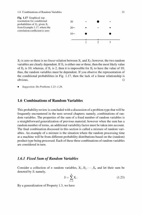
1.6 Combinations of Random Variables 31
Fig. 1.17 Graphical rep-resentation for conditionalprobabilities of X2 given X1from Example 1.17, where thecorrelation coefficient is zero
10
20
30
1 2 3
�
�
�
�
�
�
�
�
X2 is zero so there is no linear relation between X1 and X2; however, the two randomvariables are clearly dependent. If X1 is either one or three, then the most likely valueof X2 is 10; whereas, if X1 is 2, then it is impossible for X2 to have the value of 10;thus, the random variables must be dependent. If you observe the representation ofthe conditional probabilities in Fig. 1.17, then the lack of a linear relationship isobvious. ��
• Suggestion: Do Problems 1.21–1.26.
1.6 Combinations of Random Variables
This probability review is concluded with a discussion of a problem type that will befrequently encountered in the next several chapters; namely, combinations of ran-dom variables. The properties of the sum of a fixed number of random variables isa straightforward generalization of previous material; however when the sum has arandom number of terms, an additional variability factor must be taken into account.The final combination discussed in this section is called a mixture of random vari-ables. An example of a mixture is the situation where the random processing timeat a machine will be from different probability distributions based on the (random)product type being processed. Each of these three combinations of random variablesare considered in turn.
1.6.1 Fixed Sum of Random Variables
Consider a collection of n random variables, X1,X2, · · · ,Xn and let their sum bedenoted by S; namely,
S =n
∑i=1
Xi . (1.23)
By a generalization of Property 1.3, we have
32 1 Basic Probability Review
E[S] = E[X1 +X2 + · · ·+Xn]= E[X1]+E[X2]+ · · ·+E[Xn] . (1.24)
Note that (1.24) is valid even if the random variables are not independent.The variance of the random variable S is obtained in a similar manner to the
expected value
V [S] = E[(S−E[S])2]= E[S2]−E[Y ]2
= E[(X1 +X2 + · · ·+Xn)2]− (E[X1]+E[X2]+ · · ·+E[Xn])2
=n
∑i=1
E[X2i ]+2
n
∑i=1
n
∑j>i
E[XiXj]− (E[X1]+E[X2]+ · · ·+E[Xn])2
=n
∑i=1
(
E[X2i ]−E[Xi]2
)
+2n
∑i=1
n
∑j>i
(E[XiXj]−E[Xi]E[Xj])
=n
∑i=1
V [Xi]+2n
∑i=1
n
∑j>i
cov[Xi,Xj] . (1.25)
Notice that when the random variables are pair-wise independent, i.e., Xi and Xj areindependent for all i and j, then E[XiXj] = E[Xi]E[Xj] and Property 1.6 is general-ized indicating that the variance of the sum of n independent random variables is thesum of the individual variances. In addition, when X1, · · · ,Xn are independent andidentically distributed (called i.i.d.), we have that
E[S] = nE[X1] (1.26)
V [S] = nV [X1] .
1.6.2 Random Sum of Random Variables
Before discussing the random sum of random variables, we need a property of con-ditional expectations. For this discussion we follow the development in [4] in whichthese properties are developed assuming discrete random variables because the dis-crete case is more intuitive than the continuous case. (Although the developmentbelow only considers the discrete case, our main result — given as Property 1.8 —is true for both discrete and continuous random variables.)
Let Y and X be two random variables. The conditional probability that the ran-dom variable Y takes on a value b given that the random variable X takes the valuea is written as
Pr{Y = b|X = a} =Pr{Y = b,X = a}
Pr{X = a} , if Pr{X = a} �= 0

1.6 Combinations of Random Variables 33
(see Definition 1.16). Thus, the conditional expectation of Y given that X = achanges as the value a changes so it is a function, call it g, of a; namely,
E[Y |X = a] = ∑b
b Pr{Y = b|X = a} = g(a) .
Hence, the conditional expectation of Y given X is a random variable since it de-pends on the value of X , expressed as
E[Y |X ] = g(X) . (1.27)
Taking the expectation on both sides of (1.27), yields the (unconditional) expecta-tion of Y and gives the following important property.
Property 1.8. Let Y and X be any two random variables with finite expec-tation. The conditional expectation of Y given X is a random variable withexpectation given by
E [E[Y |X ] ] = E[Y ] .
Property 1.8 can now be used to obtain the properties of a random sum of randomvariables. Let S be defined by
S =N
∑i=1
Xi ,
where X1,X2, · · · is a sequence of i.i.d. random variables, and N is a nonnegativediscrete random variable independent of each Xi. (When N = 0, the random sum isinterpreted to be zero.) For a fixed n, Eq. (1.26) yields
E
[
N
∑i=1
Xi|N = n
]
= nE[X1] , thus
E
[
N
∑i=1
Xi|N]
= NE[X1] .
The expected value of the random sum can be derived from the above result usingProperty 1.8 regarding conditional expectations as follows:
E[S] = E
[
E
[
N
∑i=1
Xi|N]]
= E[NE[X1] ]= E[N]E[X1] .

34 1 Basic Probability Review
Note that the final equality in the above arises using Property 1.6 regarding inde-pendence and the fact that each random variable in an i.i.d. sequence has the samemean.
We obtain the variance of the random variable S in a similar fashion, usingV [S]=E[S2]−E[S]2 but we shall leave its derivation for homework with some hints (seeProblem 1.29). Thus, we have the following property:
Property 1.9. Let X1,X2, · · · be a sequence of i.i.d. random variables wherefor each i, E[Xi] = μ and V [Xi] = σ2. Let N be a nonnegative discrete randomvariable independent of the i.i.d. sequence, and let S = ∑N
i=1 Xi. Then
E[S] = μE[N]V [S] = σ2E[N]+ μ2V [N] .
Notice that the squared coefficient of variation of the random sum can also be easilywritten as
C2[S] = C2[N]+C2[S]E[N]
.
1.6.3 Mixtures of Random Variables
The final type of random variable combination that we consider is a mixture of ran-dom variables. For example, consider two products processed on the same machine,where the two product types have different processing characteristics. Specifically,let X1 and X2 denote the random processing times for types 1 and 2, respectively, andthen let T denote the processing time for an arbitrarily chosen part. The processingsequence will be assumed to be random with p1 and p2 being the probability thattype 1 and type 2, respectively, are to be processed. In other words, T will equal X1
with probability p1 and T will equal X2 with probability p2. Intuitively, we have thefollowing relationship.
T ={
X1 with probability p1,X2 with probability 1− p1 .
Thus, T is said to be a mixture of X1 and X2. In generalizing this concept, we havethe following definition.
Definition 1.21. Let X1, · · · ,Xn be a sequence of independent random variables andlet I be a positive discrete random variable with range 1, · · · ,n independent of theX1, · · · ,Xn sequence. The random variable T is called a mixture of random variableswith index I if it can be written as
T = XI .
Appendix 35
Making use of Property 1.8, it should not be too difficult to show the followingproperty.
Property 1.10. Let T be a mixture of X1, · · · ,Xn where the mean of Xi is μi
and variance of Xi is σ2i . Then
E[T ] =n
∑i=1
piμi
E[T 2] =n
∑i=1
pi(
σ2i + μ2
i
)
,
where Pr{I = i}= pi are the probabilities associated with the index.
Notice that the above property gives the first and second moment, not the variancedirectly. If the variance is desired, the equation V [T ] = E[T 2]−E[T ]2 must be used.
• Suggestion: Do Problems 1.27–1.29.
Appendix
In this appendix, two numerical problems are discussed: the computation of thegamma function (Eq. 1.18) and the determination of the shape and scale parametersfor the Weibull distribution. We give suggestions for those using Microsoft Exceland those who are interested in doing the computations within a programming en-vironment.
The gamma function: For Microsoft Excel users, the gamma function is eval-uated by first obtaining the natural log of the function since Excel provides anautomatic function for the log of the gamma instead of the gamma function it-self. For example, to obtain the gamma function evaluated at 1.7, use the formula"=EXP(GAMMALN(1.7))". This yields a value of 0.908639.
For programmers who need the gamma function, there are some good approxi-mations are available. A polynomial approximation taken from [5, p. 155] is
Γ (1 + x) ≈ 1 +a1x+a2x2 + · · ·+a5x5 for 0 ≤ x ≤ 1, (1.28)
where the constants are a1 =−0.5748646, a2 = 0.9512363, a3 =−0.6998588, a4 =0.4245549,and a5 =−0.1010678. (Or if you need additional accuracy, an eight termapproximation is also available in [5] or [1, p. 257].) If it is necessary to evaluateΓ (x) for x < 1 then use the relationship
Γ (x) =1x
Γ (1 + x) . (1.29)
36 1 Basic Probability Review
If it is necessary to evaluate Γ (n+x) for n > 1 and 0 ≤ x ≤ 1, then use the relation-ship:
Γ (n + x) = (n−1 + x)(n−2 + x) · · ·(1 + x)Γ (1 + x) . (1.30)
Example 1.18. Suppose we wish to compute Γ (0.7). The approximation givenby (1.28), yields a result of Γ (1.7) = 0.9086. Applying (1.29) yields Γ (0.7) =0.9086/0.7= 1.298. Now suppose that we wish to obtain the gamma function eval-uated at 5.7. From (1.30), we have Γ (5.7)= 4.7×3.7×2.7×1.7×0.9086= 72.52.
��Weibull parameters: The context for this section is that we know the first two
moments of a Weibull distribution (1.20) and would like to determine the shape andscale parameters. Notice that the SCV can be written as C2[X ] = E[X2]/(E[X ])2−1;thus, the shape parameter is the value of α that satisfies
C2[X ]+1 =Γ (1 +2/α)
(Γ (1 +1/α) )2 , (1.31)
and the scale parameter is then determined by
β =E[X ]
Γ (1 +1/α)(1.32)
Example 1.19. Suppose we would like to find the parameters of the Weibull randomvariable with mean 100 and standard deviation 25. We first note that C2[X ] + 1 =1.0625. We then fill in a spreadsheet with the following values and formulas.
A B1 alpha-guess 12 first moment =EXP(GAMMALN(1+1/B1))3 second moment =EXP(GAMMALN(1+2/B1))4 ratio = B3/(B2*B2)5 mean 1006 beta-value =B5/B2
The GoalSeek tool (found under the “Tools” menu in Excel 2003 and under the“What-If” button on the Data Tab for Excel 2007) is ideal for solving (1.31). WhenGoalSeek is clicked, a dialog box appears with three parameters. For the abovespreadsheet, the “Set cell” parameter is set to A4, the “To value” parameter is set to1.0625 (i.e., the value of the C2[X ]+1), and the “By changing cell” parameter isset to A1. The results should be that the A1 cell is changed to 4.503 and the A6 cellis changed to 109.6. ��
Problems
1.1. A manufacturing company ships (by truckload) its product to three differentdistribution centers on a weekly basis. Demands vary from week to week ranging
Problems 37
over 0, 1, and 2 truckloads needed at each distribution center. Conceptualize anexperiment where a week is selected and then the number of truckloads demandedat each of the three centers are recorded.(a) Describe the sample space, i.e., list all outcomes.(b) How many possible different events are there?(c) Write the event that represents a total of three truckloads are needed for the week.(d) If each event containing a single outcome has the same probability, what is theprobability that a total demand for three truckloads will occur?
1.2. A library has classified its books into fiction and nonfiction. Furthermore, allbooks can also be described as hardback and paperback. As an experiment, we shallpick a book at random and record whether it is fiction or nonfiction and whether itis paperback or hardback.(a) Describe the sample space, i.e., list all outcomes.(b) Describe the event space, i.e., list all events.(c) Define a probability measure such that the probability of picking a nonfictionpaperback is 0.15, the probability of picking a nonfiction book is 0.30, and the prob-ability of picking a fiction hardback is 0.65.(d) Using the probabilities from part (c), find the probability of picking a fictionbook given that the book chosen is known to be a paperback.
1.3. Let N be a random variable describing the number of defective items in a boxfrom Example 1.1. Draw the graph for the cumulative distribution function of N andgive its pmf.
1.4. Let X be a random variable with cumulative distribution function given by
G(a) =
⎧
⎨
⎩
0 for a < 0,a2 for 0 ≤ a < 1,1 for a ≥ 1.
.
(a) Give the pdf for X .(b) Find Pr{X ≥ 0.5}.(c) Find Pr{0.5 < X ≤ 0.75}.(d) Let X1 and X2 be independent random variables with their CDF given by G(·).Find Pr{X1 +X2 ≤ 1}.
1.5. Let T be a random variable with pdf given by
f (t) ={
0 for t < 0.5,
ke−2(t−0.5) for t ≥ 0.5..
(a) Find k.(b) Find Pr{0.25≤ T ≤ 1}.(c) Find Pr{T ≤ 1.5}.(d) Give the cumulative distribution function for T .(e) Let the independent random variables T1 and T2 have their pdf given by f (·).
38 1 Basic ProbabilityReview
Find Pr{1≤ T1+T2 ≤ 2}.(f) Let Y = X + T , where X is independent of T and is defined by the previousproblem. Give the pdf for Y .
1.6. LetU be a random variable with pdf given by
h(u) =
⎧⎪⎪⎨⎪⎪⎩
0 for u< 0,u for 0 ≤ u< 1,2−u for 1 ≤ u< 2,0 for u≥ 2.
.
(a) Find Pr{0.5<U < 1.5}.(b) Find Pr{0.5≤U ≤ 1.5}.(c) Find Pr{0 ≤ U ≤ 1.5, 0.5 ≤ U ≤ 2}. (A comma acts as an intersection and isread as an “and”.)(d) Give the cumulative distribution function for U and calculate Pr{U ≤ 1.5}−Pr{U ≤ 0.5}.1.7. An independent roofing contractor has determined that the number of jobs ob-tained for the month of September varies. From previous experience, the probabil-ities of obtaining 0, 1, 2, or 3 jobs have been determined to be 0.1, 0.35, 0.30, and0.25, respectively. The profit obtained from each job is $300. What is the expectedprofit for September?
1.8. There are three investment plans for your consideration. Each plan calls foran investment of $25,000 and the return will be one year later. Plan A will return$27,500. Plan B will return $27,000 or $28,000 with probabilities 0.4 and 0.6, re-spectively. Plan C will return $24,000, $27,000, or $33,000 with probabilities 0.2,0.5, and 0.3, respectively. If your objective is tomaximize the expected return, whichplan should you choose? Are there considerations that might be relevant other thansimply the expected values?
1.9. Let the random variables A,B,C denote the returns from investment plans A,B, and C, respectively, from the previous problem. What are the mean and standarddeviations of the three random variables?
1.10. Let N be a random variable with cumulative distribution function given by
F(x) =
⎧⎪⎪⎪⎪⎨⎪⎪⎪⎪⎩
0 for x< 1,0.2 for 1 ≤ x< 2,0.5 for 2 ≤ x< 3,0.8 for 3 ≤ x< 4,1 for x≥ 4.
Find the mean and standard deviation of N .
1.11. Prove that the E[(X − μ)2] = E[X2]− μ2 for any random variable X whosemean is μ.
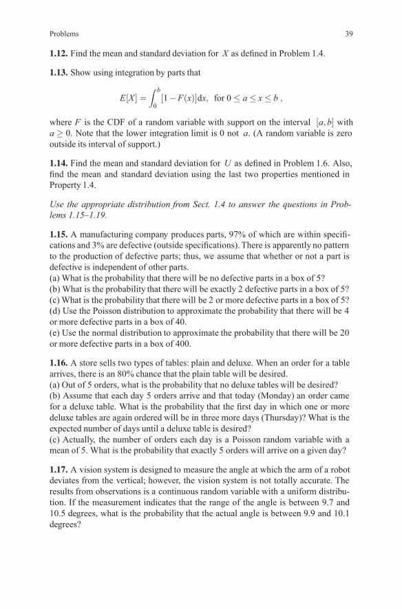
Problems 39
1.12. Find the mean and standard deviation for X as defined in Problem 1.4.
1.13. Show using integration by parts that
E[X ] =∫ b
0[1−F(x)]dx, for 0 ≤ a≤ x≤ b ,
where F is the CDF of a random variable with support on the interval [a,b] witha ≥ 0. Note that the lower integration limit is 0 not a. (A random variable is zerooutside its interval of support.)
1.14. Find the mean and standard deviation for U as defined in Problem 1.6. Also,find the mean and standard deviation using the last two properties mentioned inProperty 1.4.
Use the appropriate distribution from Sect. 1.4 to answer the questions in Prob-lems 1.15–1.19.
1.15. A manufacturing company produces parts, 97% of which are within specifi-cations and 3% are defective (outside specifications). There is apparently no patternto the production of defective parts; thus, we assume that whether or not a part isdefective is independent of other parts.(a) What is the probability that there will be no defective parts in a box of 5?(b) What is the probability that there will be exactly 2 defective parts in a box of 5?(c) What is the probability that there will be 2 or more defective parts in a box of 5?(d) Use the Poisson distribution to approximate the probability that there will be 4or more defective parts in a box of 40.(e) Use the normal distribution to approximate the probability that there will be 20or more defective parts in a box of 400.
1.16. A store sells two types of tables: plain and deluxe. When an order for a tablearrives, there is an 80% chance that the plain table will be desired.(a) Out of 5 orders, what is the probability that no deluxe tables will be desired?(b) Assume that each day 5 orders arrive and that today (Monday) an order camefor a deluxe table. What is the probability that the first day in which one or moredeluxe tables are again ordered will be in three more days (Thursday)? What is theexpected number of days until a deluxe table is desired?(c) Actually, the number of orders each day is a Poisson random variable with amean of 5. What is the probability that exactly 5 orders will arrive on a given day?
1.17. A vision system is designed to measure the angle at which the arm of a robotdeviates from the vertical; however, the vision system is not totally accurate. Theresults from observations is a continuous random variable with a uniform distribu-tion. If the measurement indicates that the range of the angle is between 9.7 and10.5 degrees, what is the probability that the actual angle is between 9.9 and 10.1degrees?
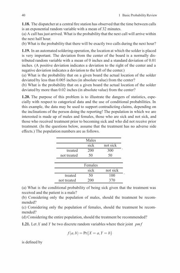
40 1 Basic ProbabilityReview
1.18. The dispatcher at a centralfire station has observed that the time between callsis an exponential random variable with a mean of 32 minutes.(a) A call has just arrived. What is the probability that the next call will arrive withinthe next half hour.(b) What is the probability that there will be exactly two calls during the next hour?
1.19. In an automated soldering operation, the location at which the solder is placedis very important. The deviation from the center of the board is a normally dis-tributed random variable with a mean of 0 inches and a standard deviation of 0.01inches. (A positive deviation indicates a deviation to the right of the center and anegative deviation indicates a deviation to the left of the center.)(a) What is the probability that on a given board the actual location of the solderdeviated by less than 0.005 inches (in absolute value) from the center?(b) What is the probability that on a given board the actual location of the solderdeviated by more than 0.02 inches (in absolute value) from the center?
1.20. The purpose of this problem is to illustrate the dangers of statistics, espe-cially with respect to categorical data and the use of conditional probabilities. Inthis example, the data may be used to support contradicting claims, depending onthe inclinations of the person doing the reporting! The population in which we areinterested is made up of males and females, those who are sick and not sick, andthose who received treatment prior to becoming sick and who did not receive priortreatment. (In the questions below, assume that the treatment has no adverse sideeffects.) The population numbers are as follows.
Malessick not sick
treated 200 300not treated 50 50
.
Femalessick not sick
treated 50 100not treated 200 370
.
(a) What is the conditional probability of being sick given that the treatment wasreceived and the patient is a male?(b) Considering only the population of males, should the treatment be recom-mended?(c) Considering only the population of females, should the treatment be recom-mended?(d) Considering the entire population, should the treatment be recommended?
1.21. Let X and Y be two discrete random variables where their joint pm f
f (a,b) = Pr{X = a,Y = b}
is defined by
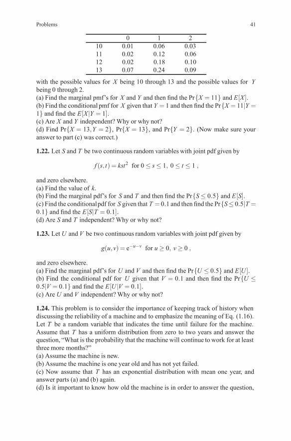
Problems 41
0 1 210 0.01 0.06 0.0311 0.02 0.12 0.0612 0.02 0.18 0.1013 0.07 0.24 0.09
with the possible values for X being 10 through 13 and the possible values for Ybeing 0 through 2.(a) Find the marginal pmf’s for X and Y and then find the Pr{X = 11} and E[X ].(b) Find the conditional pmf for X given that Y = 1 and then find the Pr{X = 11|Y =1} and find the E[X |Y = 1].(c) Are X and Y independent?Why or why not?(d) Find Pr{X = 13,Y = 2}, Pr{X = 13}, and Pr{Y = 2}. (Now make sure youranswer to part (c) was correct.)
1.22. Let S and T be two continuous random variables with joint pdf given by
f (s, t) = kst2 for 0 ≤ s≤ 1, 0≤ t ≤ 1 ,
and zero elsewhere.(a) Find the value of k.(b) Find the marginal pdf’s for S and T and then find the Pr{S≤ 0.5} and E[S].(c) Find the conditionalpdf for S given that T = 0.1 and then find the Pr{S≤ 0.5|T =0.1} and find the E[S|T = 0.1].(d) Are S and T independent?Why or why not?
1.23. LetU and V be two continuous random variables with joint pdf given by
g(u,v) = e−u−v for u≥ 0, v≥ 0 ,
and zero elsewhere.(a) Find the marginal pdf’s for U and V and then find the Pr{U ≤ 0.5} and E[U ].(b) Find the conditional pdf for U given that V = 0.1 and then find the Pr{U ≤0.5|V = 0.1} and find the E[U |V = 0.1].(c) Are U and V independent?Why or why not?
1.24. This problem is to consider the importance of keeping track of history whendiscussing the reliability of a machine and to emphasize the meaning of Eq. (1.16).Let T be a random variable that indicates the time until failure for the machine.Assume that T has a uniform distribution from zero to two years and answer thequestion, “What is the probability that the machine will continue to work for at leastthree more months?”(a) Assume the machine is new.(b) Assume the machine is one year old and has not yet failed.(c) Now assume that T has an exponential distribution with mean one year, andanswer parts (a) and (b) again.(d) Is it important to know how old the machine is in order to answer the question,
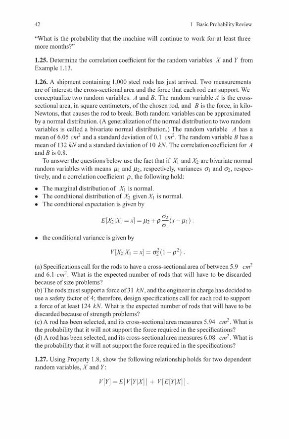
42 1 Basic ProbabilityReview
“What is the probability that the machine will continue to work for at least threemore months?”
1.25. Determine the correlation coefficient for the random variables X and Y fromExample 1.13.
1.26. A shipment containing 1,000 steel rods has just arrived. Two measurementsare of interest: the cross-sectional area and the force that each rod can support. Weconceptualize two random variables: A and B. The random variable A is the cross-sectional area, in square centimeters, of the chosen rod, and B is the force, in kilo-Newtons, that causes the rod to break. Both random variables can be approximatedby a normal distribution. (A generalizationof the normal distribution to two randomvariables is called a bivariate normal distribution.) The random variable A has amean of 6.05 cm2 and a standard deviation of 0.1 cm2. The random variable B has amean of 132 kN and a standard deviation of 10 kN. The correlation coefficient for Aand B is 0.8.To answer the questions below use the fact that if X1 and X2 are bivariate normal
random variables with means μ1 and μ2, respectively, variances σ1 and σ2, respec-tively, and a correlation coefficient ρ , the following hold:
• The marginal distribution of X1 is normal.• The conditional distribution of X2 given X1 is normal.• The conditional expectation is given by
E[X2|X1 = x] = μ2+ρσ2σ1
(x−μ1) .
• the conditional variance is given by
V [X2|X1 = x] = σ22 (1−ρ2) .
(a) Specifications call for the rods to have a cross-sectionalarea of between 5.9 cm2and 6.1 cm2. What is the expected number of rods that will have to be discardedbecause of size problems?(b) The rodsmust support a force of 31 kN, and the engineer in charge has decided touse a safety factor of 4; therefore, design specifications call for each rod to supporta force of at least 124 kN. What is the expected number of rods that will have to bediscarded because of strength problems?(c) A rod has been selected, and its cross-sectional areameasures 5.94 cm2. What isthe probability that it will not support the force required in the specifications?(d) A rod has been selected, and its cross-sectionalarea measures 6.08 cm2. What isthe probability that it will not support the force required in the specifications?
1.27. Using Property 1.8, show the following relationship holds for two dependentrandom variables, X and Y :
V [Y ] = E[V [Y |X ] ] + V [E[Y |X ] ] .
References 43
1.28. Let X1 and X2 be two independent Bernoulli random variables with E[X1] =0.8 and E[X2] = 0.6. Let S= X1+X2.(a) Give the joint pmf for S and X1.(b) Give the marginal pmf for S.(c) Give the correlation coefficient for S and X1.(d) Give the conditional pmf for S given X1 = 0 and X1 = 1.(e) Demonstrate that Property 1.8 is true where Y = S and X = X1.(f) Demonstrate that the property given in Problem 1.27 is true where Y = S andX = X1.
1.29. Derive the expression for the variance in Property 1.9. For this proof, you willneed to use the following two equations:
E[S2] = E
⎡⎣E
⎡⎣
(N
∑i=1Xi
)2|N
⎤⎦⎤⎦ ,
and
E
⎡⎣(
n
∑i=1Xi
)2⎤⎦ = E
[n
∑i=1X2i +
n
∑i=1
∑j �=iXiXj
].
References
1. Abramowitz, M., and Stegun, I.A., editors (1970). Handbook of Mathematical Functions ,Dover Publications, Inc., New York.
2. Barlow, R.E., and Proschan, F. (1975). Statistical Theory of Reliability and Life Testing , Holt,Rinehart and Winston, Inc., New York.
3. Feldman, R.M., and Valdez-Flores, C. (1996). Applied Probability & Stochastic Processes ,PWS Publishing Company, Boston.
4. Cinlar, E. (1975). Introduction to Stochastic Processes , Prentice-Hall, Inc., Englewood Cliffs,NJ.
5. Hastings, Jr., C. (1955). Approximations for Digital Computers , Princeton University Press,Princeton, NJ.
6. Law, M., and Kelton, W.D. (1991). SimulationModeling and Analysis , 2nd edition, McGraw-Hill Book Company, New York.
7. Rahman, N.A. (1968). A Course in Theoretical Statistics , Hafner Publishing Co., New York.

Chapter 2Introduction to Factory Models
An analytical approach to the modeling and analysis of manufacturing and produc-tion systems is the cornerstone of the ability to quickly evaluate alternatives (calledrapid scenario analysis) and is the emphasis of the material in this textbook. Perti-nent factors must be identified while secondary factors will generally be ignored.Starting with extremely simple models (essentially single machine/resource mod-els), the necessary mechanics and concepts needed to model these situations aredeveloped. Then more complex models are developed by connecting simple modelsinto networks of workstations with the appropriate interconnections. The overall ap-proach is to decompose a system into small components, model these components,and then reintegrate the general system by the appropriate combination of the com-ponents’ submodels. This decomposition approach is an approximation procedurethat has given acceptable results in a wide variety of manufacturing applications. Inreality any analytical model, whether exact or approximate, is an approximation ofthe real world environment. The question that must be answered is whether or notthe model yields accurate enough results to be used as an analysis tool in support ofdesign and operational decision making.
2.1 The Basics
The modeling perspective or scope throughout this textbook will start when jobsarrive to the system and end when they are completed. The model scope, depictedin Figure 2.1, will not take into account where or why jobs arrive or how they aretransported to customers. Thus, modeling the order creation or completed job deliv-ery systems is not within the scope of our analysis. It is important to observe thatwe use the term “job” loosely. An arriving job may be a physical entity that must beprocessed through the various processing steps or an arriving job may be an orderto begin the processing of (on-hand) raw material into a newly manufactured entity.
45
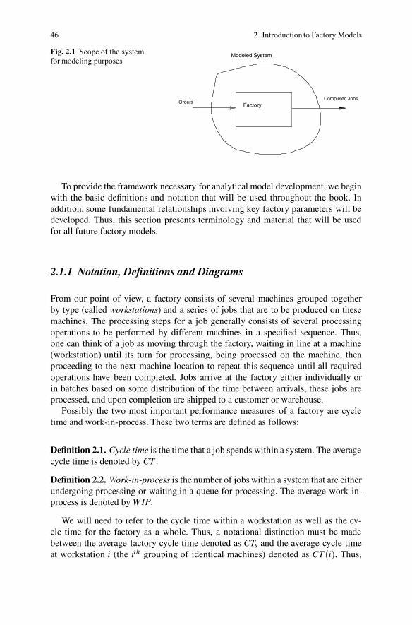
46 2 Introduction to Factory Models
Fig. 2.1 Scope of the systemfor modeling purposes
OrdersCompleted Jobs
Factory
Modeled System
To provide the framework necessary for analytical model development, we beginwith the basic definitions and notation that will be used throughout the book. Inaddition, some fundamental relationships involving key factory parameters will bedeveloped. Thus, this section presents terminology and material that will be usedfor all future factory models.
2.1.1 Notation, Definitions and Diagrams
From our point of view, a factory consists of several machines grouped togetherby type (called workstations) and a series of jobs that are to be produced on thesemachines. The processing steps for a job generally consists of several processingoperations to be performed by different machines in a specified sequence. Thus,one can think of a job as moving through the factory, waiting in line at a machine(workstation) until its turn for processing, being processed on the machine, thenproceeding to the next machine location to repeat this sequence until all requiredoperations have been completed. Jobs arrive at the factory either individually orin batches based on some distribution of the time between arrivals, these jobs areprocessed, and upon completion are shipped to a customer or warehouse.
Possibly the two most important performance measures of a factory are cycletime and work-in-process. These two terms are defined as follows:
Definition 2.1. Cycle time is the time that a job spends within a system. The averagecycle time is denoted by CT .
Definition 2.2. Work-in-process is the number of jobs within a system that are eitherundergoing processing or waiting in a queue for processing. The average work-in-process is denoted by W IP.
We will need to refer to the cycle time within a workstation as well as the cy-cle time for the factory as a whole. Thus, a notational distinction must be madebetween the average factory cycle time denoted as CTs and the average cycle timeat workstation i (the ith grouping of identical machines) denoted as CT (i). Thus,
2.1 The Basics 47
CTs is the average time that a job spends within the factory, either being processedat a workstation or waiting in a workstation queue; whereas, CT (i) is the averagetime jobs spend being processed by workstation i plus the average time spend in theworkstation i queue (or buffer). At times, general properties related to the averagecycle time will be developed, in which case CT is used without subscript. At otherit will be important to specifically refer to the average cycle time at a workstation orwithin the entire factory, in which case either CT (i) or CTs will be used.
To add to the notational confusion, the cycle time at a machine consists of twocomponents, the processing time and the waiting time or queue time at the machineuntil its processing begins. The processing time at a machine is often known orcan be determined without much effort; however, the queue time at a machine is noteasily estimated for a given job since it depends on the number and processing timesof the various types of jobs that are waiting in the queue ahead of the designated job.Thus, the average cycle time at workstation i is given as the sum of two components;namely,
CT (i) = CTq(i)+E[Ts(i)] , (2.1)
where CTq(i) denotes the average time a job spends in the queue in front of theworkstation and Ts(i) denotes the service time (or processing time) at workstation i.(We have just introduced a potential source of confusion in notation, but it shouldhelp in future chapters. The “s” subscript usually refers to a “system” characteristic;however, for the random variable T , the subscript refers to “service”. The reason forthis is that it will become necessary to distinguish among arrival times, departuretimes, and service times in later chapters.)
Another key system performance measure is the throughput rate.
Definition 2.3. The throughput rate for a system is the number of completed jobsleaving the system per unit of time. The throughput rate averaged over many jobs isdenoted by th.
For most of the systems that we will consider, the long-run throughput rate of thesystem must be equal to the input rate of jobs. Given that the throughput rate isknown, the main issue will then be the estimation of the total length of time for themanufacturing process (CTs). Given that there is enough capacity to satisfy the longterm average demand, the average cycle time in the factory or system is a functionof the factory’s capacity relative to the minimum capacity needed. The higher thefactory capacity relative to the needs, the faster jobs are completed. Thus, cycle timeincreases as the factory becomes busier.
As mentioned above, a workstation can be either be a single machine or multiplemachines.
Definition 2.4. A workstation (or machine group) is a collection of one or moreidentical machines or resources.
Non-identical machines will not generally be grouped together into a single work-station for purposes of analysis in this text. Also only one type of resource is consid-ered at each workstation. For example, a system that has an operator handling more
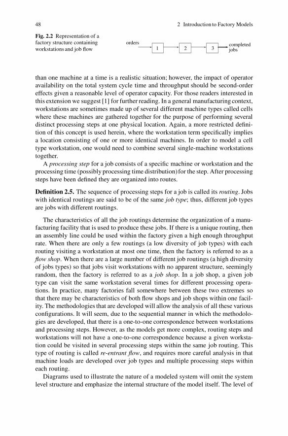
48 2 Introduction to Factory Models
Fig. 2.2 Representation of afactory structure containingworkstations and job flow 1 2 3
orders completedjobs
than one machine at a time is a realistic situation; however, the impact of operatoravailability on the total system cycle time and throughput should be second-ordereffects given a reasonable level of operator capacity. For those readers interested inthis extension we suggest [1] for further reading. In a general manufacturing context,workstations are sometimes made up of several different machine types called cellswhere these machines are gathered together for the purpose of performing severaldistinct processing steps at one physical location. Again, a more restricted defini-tion of this concept is used herein, where the workstation term specifically impliesa location consisting of one or more identical machines. In order to model a celltype workstation, one would need to combine several single-machine workstationstogether.
A processing step for a job consists of a specific machine or workstation and theprocessing time (possibly processing time distribution)for the step. After processingsteps have been defined they are organized into routes.
Definition 2.5. The sequence of processing steps for a job is called its routing. Jobswith identical routings are said to be of the same job type; thus, different job typesare jobs with different routings.
The characteristics of all the job routings determine the organization of a manu-facturing facility that is used to produce these jobs. If there is a unique routing, thenan assembly line could be used within the factory given a high enough throughputrate. When there are only a few routings (a low diversity of job types) with eachrouting visiting a workstation at most one time, then the factory is referred to as aflow shop. When there are a large number of different job routings (a high diversityof jobs types) so that jobs visit workstations with no apparent structure, seeminglyrandom, then the factory is referred to as a job shop. In a job shop, a given jobtype can visit the same workstation several times for different processing opera-tions. In practice, many factories fall somewhere between these two extremes sothat there may be characteristics of both flow shops and job shops within one facil-ity. The methodologies that are developed will allow the analysis of all these variousconfigurations. It will seem, due to the sequential manner in which the methodolo-gies are developed, that there is a one-to-one correspondence between workstationsand processing steps. However, as the models get more complex, routing steps andworkstations will not have a one-to-one correspondence because a given worksta-tion could be visited in several processing steps within the same job routing. Thistype of routing is called re-entrant flow, and requires more careful analysis in thatmachine loads are developed over job types and multiple processing steps withineach routing.
Diagrams used to illustrate the nature of a modeled system will omit the systemlevel structure and emphasize the internal structure of the model itself. The level of
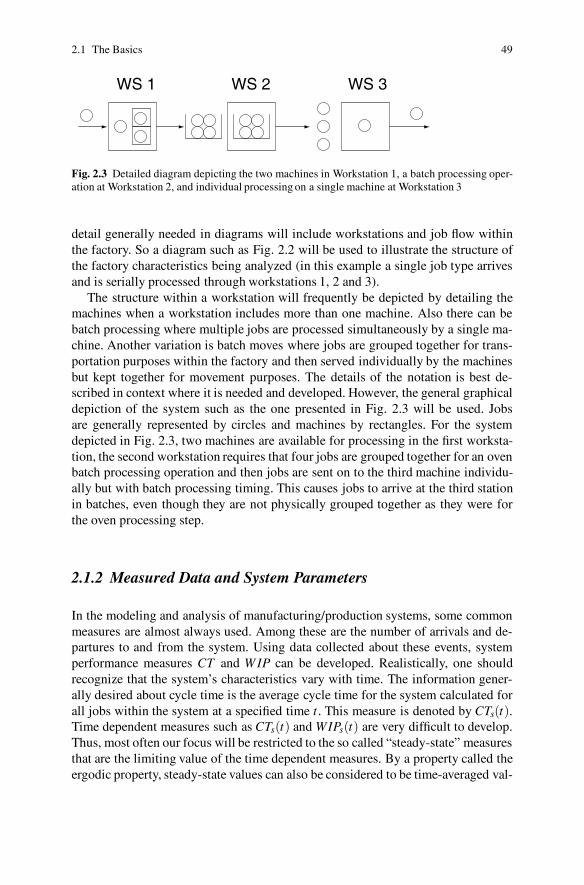
2.1 The Basics 49
WS 1 WS 2 WS 3
Fig. 2.3 Detailed diagram depicting the two machines in Workstation 1, a batch processing oper-ation at Workstation 2, and individual processing on a single machine at Workstation 3
detail generally needed in diagrams will include workstations and job flow withinthe factory. So a diagram such as Fig. 2.2 will be used to illustrate the structure ofthe factory characteristics being analyzed (in this example a single job type arrivesand is serially processed through workstations 1, 2 and 3).
The structure within a workstation will frequently be depicted by detailing themachines when a workstation includes more than one machine. Also there can bebatch processing where multiple jobs are processed simultaneously by a single ma-chine. Another variation is batch moves where jobs are grouped together for trans-portation purposes within the factory and then served individually by the machinesbut kept together for movement purposes. The details of the notation is best de-scribed in context where it is needed and developed. However, the general graphicaldepiction of the system such as the one presented in Fig. 2.3 will be used. Jobsare generally represented by circles and machines by rectangles. For the systemdepicted in Fig. 2.3, two machines are available for processing in the first worksta-tion, the second workstation requires that four jobs are grouped together for an ovenbatch processing operation and then jobs are sent on to the third machine individu-ally but with batch processing timing. This causes jobs to arrive at the third stationin batches, even though they are not physically grouped together as they were forthe oven processing step.
2.1.2 Measured Data and System Parameters
In the modeling and analysis of manufacturing/production systems, some commonmeasures are almost always used. Among these are the number of arrivals and de-partures to and from the system. Using data collected about these events, systemperformance measures CT and W IP can be developed. Realistically, one shouldrecognize that the system’s characteristics vary with time. The information gener-ally desired about cycle time is the average cycle time for the system calculated forall jobs within the system at a specified time t . This measure is denoted by CTs(t).Time dependent measures such as CTs(t) and WIPs(t) are very difficult to develop.Thus, most often our focus will be restricted to the so called “steady-state” measuresthat are the limiting value of the time dependent measures. By a property called theergodic property, steady-state values can also be considered to be time-averaged val-
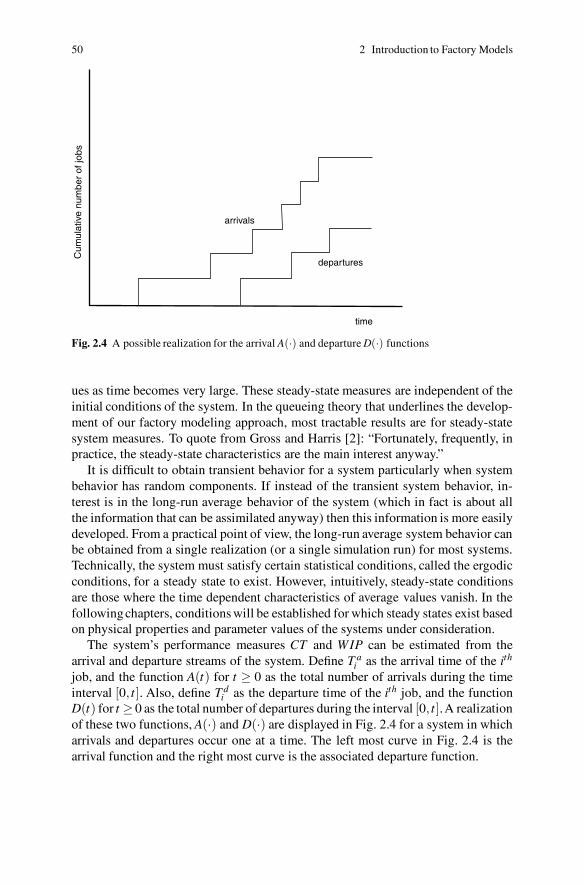
50 2 Introduction to Factory Models
time
Cum
ulat
ive
num
ber
of jo
bs
arrivals
departures
Fig. 2.4 A possible realization for the arrival A(·) and departure D(·) functions
ues as time becomes very large. These steady-state measures are independent of theinitial conditions of the system. In the queueing theory that underlines the develop-ment of our factory modeling approach, most tractable results are for steady-statesystem measures. To quote from Gross and Harris [2]: “Fortunately, frequently, inpractice, the steady-state characteristics are the main interest anyway.”
It is difficult to obtain transient behavior for a system particularly when systembehavior has random components. If instead of the transient system behavior, in-terest is in the long-run average behavior of the system (which in fact is about allthe information that can be assimilated anyway) then this information is more easilydeveloped. From a practical point of view, the long-run average system behavior canbe obtained from a single realization (or a single simulation run) for most systems.Technically, the system must satisfy certain statistical conditions, called the ergodicconditions, for a steady state to exist. However, intuitively, steady-state conditionsare those where the time dependent characteristics of average values vanish. In thefollowing chapters, conditions will be established for which steady states exist basedon physical properties and parameter values of the systems under consideration.
The system’s performance measures CT and WIP can be estimated from thearrival and departure streams of the system. Define T a
i as the arrival time of the ith
job, and the function A(t) for t ≥ 0 as the total number of arrivals during the timeinterval [0, t ]. Also, define T d
i as the departure time of the ith job, and the functionD(t) for t ≥ 0 as the total number of departures during the interval [0, t ].A realizationof these two functions, A(·) and D(·) are displayed in Fig. 2.4 for a system in whicharrivals and departures occur one at a time. The left most curve in Fig. 2.4 is thearrival function and the right most curve is the associated departure function.
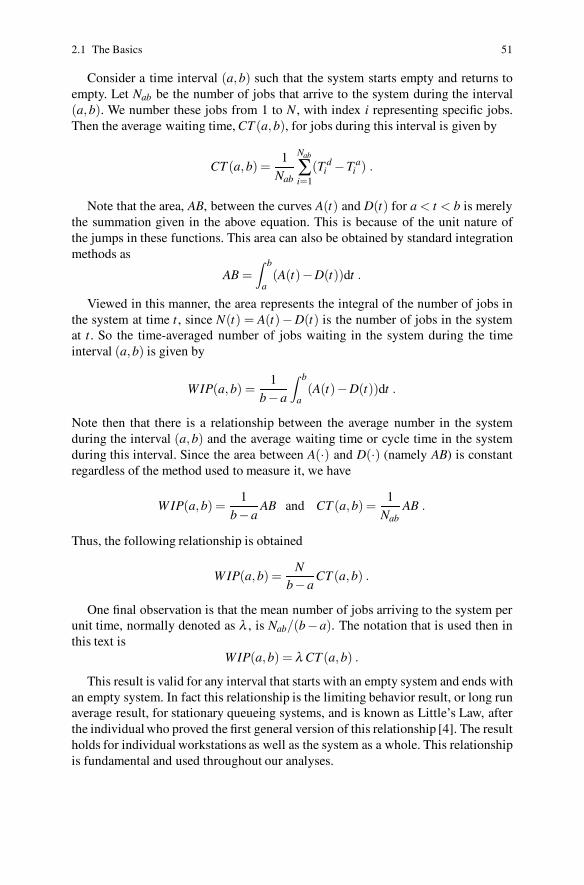
2.1 The Basics 51
Consider a time interval (a,b) such that the system starts empty and returns toempty. Let Nab be the number of jobs that arrive to the system during the interval(a,b). We number these jobs from 1 to N , with index i representing specific jobs.Then the average waiting time, CT (a,b), for jobs during this interval is given by
CT (a,b) =1
Nab
Nab
∑i=1
(T di −T a
i ) .
Note that the area, AB, between the curves A(t) and D(t) for a < t < b is merelythe summation given in the above equation. This is because of the unit nature ofthe jumps in these functions. This area can also be obtained by standard integrationmethods as
AB =∫ b
a(A(t)−D(t))dt .
Viewed in this manner, the area represents the integral of the number of jobs inthe system at time t , since N(t) = A(t)−D(t) is the number of jobs in the systemat t . So the time-averaged number of jobs waiting in the system during the timeinterval (a,b) is given by
WIP(a,b) =1
b−a
∫ b
a(A(t)−D(t))dt .
Note then that there is a relationship between the average number in the systemduring the interval (a,b) and the average waiting time or cycle time in the systemduring this interval. Since the area between A(·) and D(·) (namely AB) is constantregardless of the method used to measure it, we have
W IP(a,b) =1
b−aAB and CT (a,b) =
1Nab
AB .
Thus, the following relationship is obtained
W IP(a,b) =N
b−aCT (a,b) .
One final observation is that the mean number of jobs arriving to the system perunit time, normally denoted as λ , is Nab/(b−a). The notation that is used then inthis text is
WIP(a,b) = λ CT (a,b) .
This result is valid for any interval that starts with an empty system and ends withan empty system. In fact this relationship is the limiting behavior result, or long runaverage result, for stationary queueing systems, and is known as Little’s Law, afterthe individual who proved the first general version of this relationship [4]. The resultholds for individual workstations as well as the system as a whole. This relationshipis fundamental and used throughout our analyses.

52 2 Introduction to Factory Models
Property 2.1. Little’s Law. For a system that satisfies steady-state condi-tions, the following equation holds
W IP = λ ×CT ,
where W IP is the long-run average number of jobs in the system, CT is thelong-run average cycle time and λ is the long-run input rate of jobs to theserver.
Since the average input rate is usually equal to the average throughput rate, Lit-tle’s Law can also be written as WIP = th×CT . It should be stressed that the lim-iting behavior generally estimates mean values and the actual underlying randomvariables for the systems can be quite variable. For example in most single worksta-tion system models, the average number in the system, WIP, can be easily obtained.However, the behavior of the random variable representing the number in the systemat any one point in time can be highly variable as is illustrated in Fig. 2.5 where thenumber in the system is plotted over time from a simulation. (Note that by our defi-nition,W IP is the steady-state value of the mean of the random variable representingthe number in the system.)
Also of importance is the fact that the term steady-state implies that the meanreaches a limiting value and thus ceases to change with respect to time. However,steady-state does not imply that the system itself ceases to change; the variabilityas shown in Fig. 2.5 continues forever (i.e., the fluctuations within the system nevercease). Steady-state does imply that the entire distribution reaches a limiting valueso that not only the mean but also the standard deviation, skewness, and other suchmeasures will have limiting values.
It is often desired that analytical models of these systems describe the steady-state probability distribution. The various measures such as the mean and varianceare then computed using the derived distribution. System WIPs is a good exampleof one such measure. For a single server system with exponential inter-arrival times(of mean rate λ ) and exponential service times (of mean rate μ), the steady-stateprobability of n jobs in the system is given by
Pr{N = n} =(
1− λμ
)(
λμ
)n
for n = 0,1, · · · ,∞ ,
where N is the long-run number of jobs within the system. This result is developedin the next chapter.
The mean number of jobs in the system (WIPs) is the expected value of thisdiscrete probability distribution,
WIPs = E[N] =∞
∑n=0
npn, (2.2)
which yields

2.1 The Basics 53
Fig. 2.5 A representation of the number of jobs in a simulated factory
W IPs =λ/μ
(1−λ/μ), given that λ < μ .
Note that the condition, λ < μ, establishes the existence of a steady-state for thissystem. Using Little’s Law (Definition 2.1), the expected time in the system or cycletime, CTs, becomes
CTs =1
μ −λ.
The goal of our modeling efforts in future chapters will be to develop equationssuch as the above. Often, the long-run distribution will be derived and then the meanmeasures will be obtained from the distributions. The next chapter addresses singleworkstation models and the associated queueing theory mechanics for their devel-opment and approximation.
• Suggestion: Do Problems 2.1–2.2.
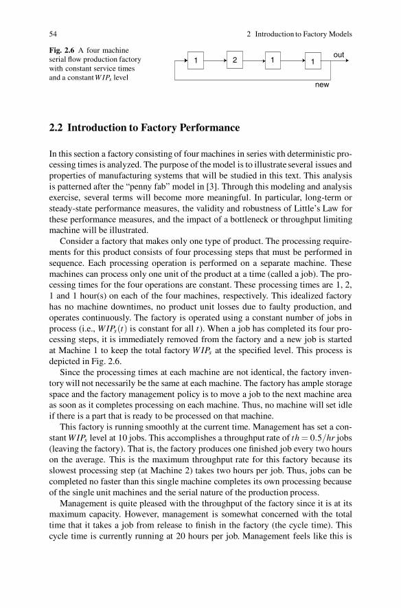
54 2 Introduction to Factory Models
Fig. 2.6 A four machineserial flow production factorywith constant service timesand a constantW IPs level
new
out1 2 1 1
2.2 Introduction to Factory Performance
In this section a factory consisting of four machines in series with deterministic pro-cessing times is analyzed. The purpose of the model is to illustrate several issues andproperties of manufacturing systems that will be studied in this text. This analysisis patterned after the “penny fab” model in [3]. Through this modeling and analysisexercise, several terms will become more meaningful. In particular, long-term orsteady-state performance measures, the validity and robustness of Little’s Law forthese performance measures, and the impact of a bottleneck or throughput limitingmachine will be illustrated.
Consider a factory that makes only one type of product. The processing require-ments for this product consists of four processing steps that must be performed insequence. Each processing operation is performed on a separate machine. Thesemachines can process only one unit of the product at a time (called a job). The pro-cessing times for the four operations are constant. These processing times are 1, 2,1 and 1 hour(s) on each of the four machines, respectively. This idealized factoryhas no machine downtimes, no product unit losses due to faulty production, andoperates continuously. The factory is operated using a constant number of jobs inprocess (i.e., WIPs(t) is constant for all t). When a job has completed its four pro-cessing steps, it is immediately removed from the factory and a new job is startedat Machine 1 to keep the total factory W IPs at the specified level. This process isdepicted in Fig. 2.6.
Since the processing times at each machine are not identical, the factory inven-tory will not necessarily be the same at each machine. The factory has ample storagespace and the factory management policy is to move a job to the next machine areaas soon as it completes processing on each machine. Thus, no machine will set idleif there is a part that is ready to be processed on that machine.
This factory is running smoothly at the current time. Management has set a con-stant WIPs level at 10 jobs. This accomplishes a throughput rate of th = 0.5/hr jobs(leaving the factory). That is, the factory produces one finished job every two hourson the average. This is the maximum throughput rate for this factory because itsslowest processing step (at Machine 2) takes two hours per job. Thus, jobs can becompleted no faster than this single machine completes its own processing becauseof the single unit machines and the serial nature of the production process.
Management is quite pleased with the throughput of the factory since it is at itsmaximum capacity. However, management is somewhat concerned with the totaltime that it takes a job from release to finish in the factory (the cycle time). Thiscycle time is currently running at 20 hours per job. Management feels like this is

2.2 Introduction to Factory Performance 55
high since it only takes 5 hours of processing to complete each job. The ratio of thecycle time to the processing time is a standard industry measure that will be calledthe x-factor.
Definition 2.6. The x-factor for a factory is the ratio of CTs to the average totalprocessing time per job.
The average for this industry is currently running at 2.6 as reported in a recentpublication by the industry’s professional journal. With this factory’s x-factor being4, management is worried about their ability to keep customers when the industryon average produces the same product with a considerably shorter lead-time fromorder placement to receipt.
To address the cycle time problem, management has been considering a largecapital outlay to purchase a 25% faster machine (1.5 hours) for processing step two.This purchase would be made expressly for the purpose of reducing the x-factorfor the factory to be more in line with the industry average. The company sellingthe machine says that this investment will bring the x-factor down to 3.33 and theadditional throughput of 0.166 units per hour would pay for the cost of the newmachine in three years.
Management has decided that this investment is not worthwhile just based onincreased throughput because the funds needed for the large capital outlay to buythe machine are sorely needed in other aspects of the company. The life blood ofthe company has been its ability to keep pace with the competition in new productdevelopment. This level of expenditure would decimate the company’s investmentin research and development of new products.
In an effort to seek a lower cost solution to the x-factor performance measurefor the factory, a consulting team from the manufacturing engineering departmentof a local university was hired to perform a short term factory flow analysis study.The first activity of the consulting team was to devise a method of predicting thelong-term factory performance measures of cycle time and throughput.
2.2.1 The Modeling Method
The consulting team accomplished the performance estimation task rather quicklydevising a hand simulation procedure of the factory flow. They started with thespecified number of 10 jobs in the factory, all placed at Machine 1, and made hourlyupdates to each job’s status. Each job that was on a machine was allocated one hourof processing time and if this completed their requirements on that machine, the jobwas moved to the next machine. Empty machines were loaded with the first job inthe machine queue, for those with a queue, and the next hourly update was started.The jobs soon distributed themselves throughout the factory and after a short periodof time a two-hour cyclic pattern emerged. Every cycle of this pattern produced onecompleted job and the factory returned to the identical state for each machine andassociated queue. This set of conditions is referred to as the factory status.
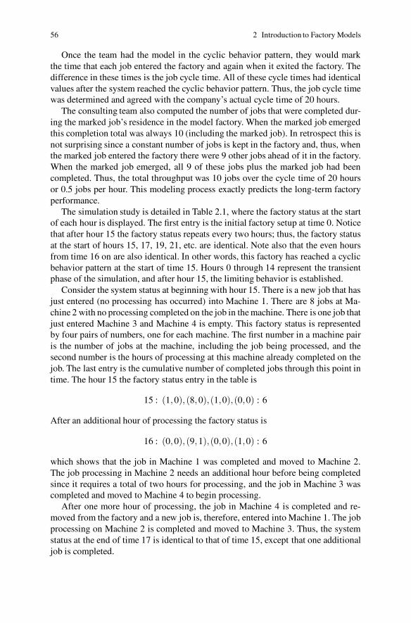
56 2 Introduction to Factory Models
Once the team had the model in the cyclic behavior pattern, they would markthe time that each job entered the factory and again when it exited the factory. Thedifference in these times is the job cycle time. All of these cycle times had identicalvalues after the system reached the cyclic behavior pattern. Thus, the job cycle timewas determined and agreed with the company’s actual cycle time of 20 hours.
The consulting team also computed the number of jobs that were completed dur-ing the marked job’s residence in the model factory. When the marked job emergedthis completion total was always 10 (including the marked job). In retrospect this isnot surprising since a constant number of jobs is kept in the factory and, thus, whenthe marked job entered the factory there were 9 other jobs ahead of it in the factory.When the marked job emerged, all 9 of these jobs plus the marked job had beencompleted. Thus, the total throughput was 10 jobs over the cycle time of 20 hoursor 0.5 jobs per hour. This modeling process exactly predicts the long-term factoryperformance.
The simulation study is detailed in Table 2.1, where the factory status at the startof each hour is displayed. The first entry is the initial factory setup at time 0. Noticethat after hour 15 the factory status repeats every two hours; thus, the factory statusat the start of hours 15, 17, 19, 21, etc. are identical. Note also that the even hoursfrom time 16 on are also identical. In other words, this factory has reached a cyclicbehavior pattern at the start of time 15. Hours 0 through 14 represent the transientphase of the simulation, and after hour 15, the limiting behavior is established.
Consider the system status at beginning with hour 15. There is a new job that hasjust entered (no processing has occurred) into Machine 1. There are 8 jobs at Ma-chine 2 with no processing completed on the job in the machine. There is one job thatjust entered Machine 3 and Machine 4 is empty. This factory status is representedby four pairs of numbers, one for each machine. The first number in a machine pairis the number of jobs at the machine, including the job being processed, and thesecond number is the hours of processing at this machine already completed on thejob. The last entry is the cumulative number of completed jobs through this point intime. The hour 15 the factory status entry in the table is
15 : (1,0), (8,0),(1,0),(0,0) : 6
After an additional hour of processing the factory status is
16 : (0,0), (9,1),(0,0),(1,0) : 6
which shows that the job in Machine 1 was completed and moved to Machine 2.The job processing in Machine 2 needs an additional hour before being completedsince it requires a total of two hours for processing, and the job in Machine 3 wascompleted and moved to Machine 4 to begin processing.
After one more hour of processing, the job in Machine 4 is completed and re-moved from the factory and a new job is, therefore, entered into Machine 1. The jobprocessing on Machine 2 is completed and moved to Machine 3. Thus, the systemstatus at the end of time 17 is identical to that of time 15, except that one additionaljob is completed.
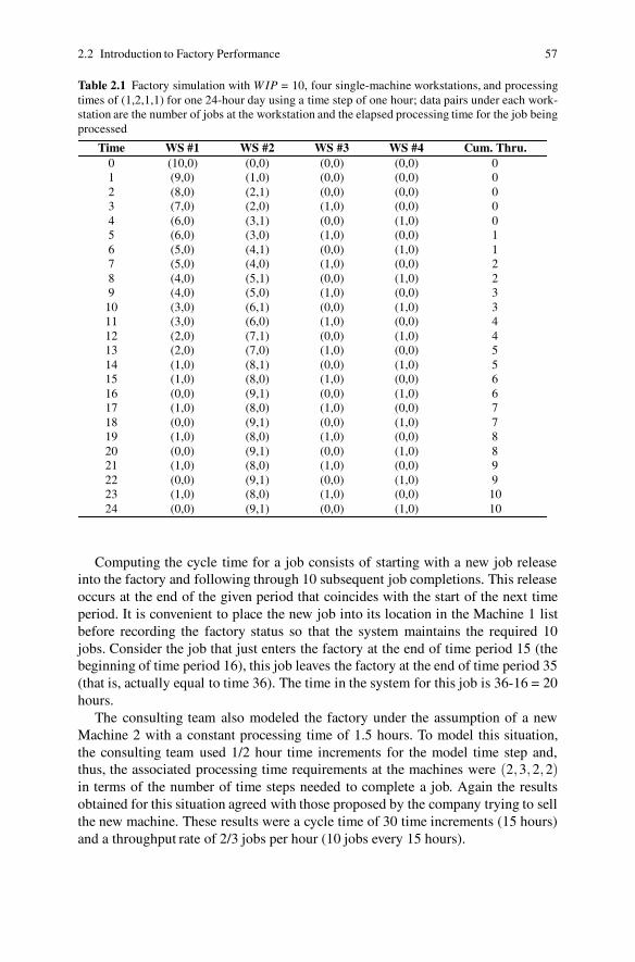
2.2 Introduction to Factory Performance 57
Table 2.1 Factory simulation with W IP = 10, four single-machine workstations, and processingtimes of (1,2,1,1) for one 24-hour day using a time step of one hour; data pairs under each work-station are the number of jobs at the workstation and the elapsed processing time for the job beingprocessed
Time WS #1 WS #2 WS #3 WS #4 Cum. Thru.0 (10,0) (0,0) (0,0) (0,0) 01 (9,0) (1,0) (0,0) (0,0) 02 (8,0) (2,1) (0,0) (0,0) 03 (7,0) (2,0) (1,0) (0,0) 04 (6,0) (3,1) (0,0) (1,0) 05 (6,0) (3,0) (1,0) (0,0) 16 (5,0) (4,1) (0,0) (1,0) 17 (5,0) (4,0) (1,0) (0,0) 28 (4,0) (5,1) (0,0) (1,0) 29 (4,0) (5,0) (1,0) (0,0) 3
10 (3,0) (6,1) (0,0) (1,0) 311 (3,0) (6,0) (1,0) (0,0) 412 (2,0) (7,1) (0,0) (1,0) 413 (2,0) (7,0) (1,0) (0,0) 514 (1,0) (8,1) (0,0) (1,0) 515 (1,0) (8,0) (1,0) (0,0) 616 (0,0) (9,1) (0,0) (1,0) 617 (1,0) (8,0) (1,0) (0,0) 718 (0,0) (9,1) (0,0) (1,0) 719 (1,0) (8,0) (1,0) (0,0) 820 (0,0) (9,1) (0,0) (1,0) 821 (1,0) (8,0) (1,0) (0,0) 922 (0,0) (9,1) (0,0) (1,0) 923 (1,0) (8,0) (1,0) (0,0) 1024 (0,0) (9,1) (0,0) (1,0) 10
Computing the cycle time for a job consists of starting with a new job releaseinto the factory and following through 10 subsequent job completions. This releaseoccurs at the end of the given period that coincides with the start of the next timeperiod. It is convenient to place the new job into its location in the Machine 1 listbefore recording the factory status so that the system maintains the required 10jobs. Consider the job that just enters the factory at the end of time period 15 (thebeginning of time period 16), this job leaves the factory at the end of time period 35(that is, actually equal to time 36). The time in the system for this job is 36-16 = 20hours.
The consulting team also modeled the factory under the assumption of a newMachine 2 with a constant processing time of 1.5 hours. To model this situation,the consulting team used 1/2 hour time increments for the model time step and,thus, the associated processing time requirements at the machines were (2,3,2,2)in terms of the number of time steps needed to complete a job. Again the resultsobtained for this situation agreed with those proposed by the company trying to sellthe new machine. These results were a cycle time of 30 time increments (15 hours)and a throughput rate of 2/3 jobs per hour (10 jobs every 15 hours).
58 2 Introduction to Factory Models
2.2.2 Model Usage
The consulting team, recognizing that their modeling approach was general and be-ing familiar with Little’s Law (W IP equals throughput multiplied by CT ), decidedto estimate the x-factor, the ratio of cycle time to total processing time, for vari-ous numbers of jobs in the system (W IP). Letting CT represent cycle time and threpresent throughput, then Little’s Law (Property 2.1) yields
CT = WIP/th.
Using a throughput rate of 1/2 jobs per hour, then cycle time is given by
CT = 2×WIP .
Since the total processing time is 5 time units, then the ratio of the cycle time to theprocessing time called the x-factor for the factory would be
x =CT5
=W IP2.5
.
Notice that as long as the processing speeds of the machines do not change, themaximum throughput rate for this factor is 1/2 per hour due to the speed of thesecond workstation. Thus, the above formula gives shows the relationship betweenthe x-factor and WIP provided that W IP does not get too small so as to “starve”Machine 2. Therefore, using the above formula, notice that if W IP = 6.5, the x-factor will equal the desired level of 2.6.
Since 6.5 is a non-integer, the constant W IP level should be set to 6 or 7. A fixedWIP level of 6 should yield an x-factor lower than 2.6 and a fixed W IP level of 7should yield an x-factor slightly higher than 2.6 as long as the throughput rate of 1/2per hour can be maintained.
The consulting team recognized that Little’s Law is a relationship between threefactory performance measures and that two of these measures must be known be-fore the third can be obtained. The issue of concern is whether or not the throughputwould stay at 1/2 when the total factory W IP was reduced below 10 jobs. For in-stance if only one job is allowed in the factory, the throughput rate is one job every5 hours or 1/5. It certainly is obvious that at some job level, the factory throughputwould drop below 1/2. So the consulting team decided to perform a study of the fac-tory performance for all fixed job levels from 1 to 10 using their performance anal-ysis modeling approach. These results are displayed in Table 2.2. They found thatthe W IP level in the factory can be reduced all the way down to 3 jobs while main-taining the factory throughput rate of 1/2. The cycle time reduces to 2×WIP = 6hours with an x-factor of 1.2. Thus at no expense, the factory can maintain its cur-rent throughput rate and reduce its cycle time from 20 to 6 hours. The cycle time andthroughput performance measures for this factory as a function of the fixed factoryWIP level are displayed in Figs. 2.7 and 2.8, respectively.

2.2 Introduction to Factory Performance 59
Fig. 2.7 Average cycle timefor the simple factory modelas a function of the constantWIP level
0 2 4 6 8 10
Constant WIP Level
0
5
10
15
20
Cyc
le T
ime
Fig. 2.8 Average throughputrate for the simple factorymodel as a function of theconstantW IP level
0 2 4 6 8 10
Constant WIP Level
0
Thr
ough
put
0.2
0.4
0.6
2.2.3 Model Conclusions
Detailed consideration has been given to the factory performance measures ofthroughput, cycle time and work-in-process for a simple factory model. Little’sLaw for long-term system behavior is valid for both deterministic and stochasticfactory models. Little’s Law applies to individual workstations and to the system as
Table 2.2 Factory performance measures as a function of the W IP level
W IP Throughput Cycle Time x-factor1 0.2 5 1.02 0.4 5 1.03 0.5 6 1.24 0.5 8 1.65 0.5 10 2.06 0.5 12 2.47 0.5 14 2.88 0.5 16 3.29 0.5 18 3.610 0.5 20 4.0
60 2 Introduction to Factory Models
a whole. For serial systems, the factory performance is controlled by the bottleneckworkstation (herein, the slowest machine). When there is enough WIP in the systemthe maximum throughput rate is reached and is equal to the bottleneck workstation(machine). As WIP increases beyond the minimum needed to reach the maximalthroughput rate, factory cycle time performance degrades proportionally.
• Suggestion: Do Problems 2.3–2.14.
2.3 Deterministic vs Stochastic Models
The simple throughput analysis of a serial factory with deterministic processingtimes of the last section was used to illustrate several system performance mea-sures and their inter-relationships (i.e., Little’s Law). The modeling approach wasdeveloped specifically for deterministic processing times. This approach does notnecessarily yield accurate results when processing times are random. If the meanprocessing time for a stochastic system is used in the above deterministic model-ing approach, the results can be misleading and the wrong decisions can be drawn.This problem is illustrated below with a system similar to the above example. Thekey point to be made here is that for the evaluation of stochastic systems, stochas-tic methodologies should be employed. How one models stochastic production andmanufacturing systems is the purpose of this book.
Consider the four-step production system represented by Fig. 2.6. Now insteadof the constant processing time of two hours at workstation 2, let us assume thatthis time actually varies between two values: 1 hour and 3 hours. If these timesoccur with equal probability, then the system has a mean processing time of 2 hoursand using this time one would draw the conclusions of the previous section. Recallthat the principle problem was to determine the constant W IP level that yields amaximal throughput rate while maintaining a cycle time that is as small as possible.The decision arrived at using the deterministic analysis was that a WIP level of 3jobs in the system at all times yields the maximum throughput rate of 0.5 jobs perhour with the minimal cycle time of 6 hours.
This stochastic system is now analyzed more thoroughly. One (incorrect) ap-proach would be to develop the system performance measures using the determinis-tic model but recognizing that the processing times at Machine 2 are not 2 hours but1 hour and 3 hours, with equal frequency. Thus, one approach would be to model thesystem using constant processing times of 1 hour and 3 hours and then average theseresults since these times occur with equal frequencies. This leads to the results inTable 2.3. These average results indicate that the decision to limit the constant W IPlevel to 3 jobs is incorrect and that 4 jobs would yield the maximum throughput of2/3 jobs per hour. Thus, this slightly more involved (but still not proper) methodol-ogy, would indicate that the throughput level is up by 33% over the previous estimateof 0.5 jobs per hour.
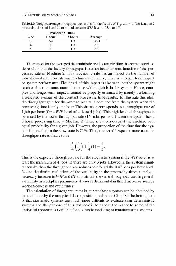
2.3 Deterministic vs Stochastic Models 61
Table 2.3 Weighed average throughput rate results for the factory of Fig. 2.6 with Workstation 2processing times of 1 and 3 hours, and constant W IP levels of 3, 4 and 5
Processing TimesW IP 1 hour 3 hours Average
3 3/4 1/3 13/244 1 1/3 2/35 1 1/3 2/3
The reason for the averaged deterministic results not yielding the correct stochas-tic result is that the factory throughput is not an instantaneous function of the pro-cessing rate of Machine 2. This processing rate has an impact on the number ofjobs allowed into downstream machines and, hence, there is a longer term impacton system performance. The length of this impact is also such that the system mightre-enter this rate status more than once while a job is in the system. Hence, com-plex and longer term impacts cannot be properly estimated by merely performinga weighted average of the constant processing time results. To illustrate this idea,the throughput gain for the average results is obtained from the system when theprocessing time is only one hour. This situation corresponds to a throughput rate of1 job per hour (for a WIP level of at least 4 jobs). This high level of throughput isbalanced by the lower throughput rate (1/3 jobs per hour) when the system has a3 hours processing time at Machine 2. These situations occur at the machine withequal probability for a given job. However, the proportion of the time that the sys-tem is operating in the slow state is 75%. Thus, one would expect a more accuratethroughput rate estimate to be
34
(
13
)
+14
(1) =12.
This is the expected throughput rate for the stochastic system if the W IP level is atleast the minimum of 4 jobs. If there are only 3 jobs allowed in the system simul-taneously, then the throughput rate reduces to around the 0.47 jobs per hour level.Notice the detrimental effect of the variability in the processing time; namely, anecessary increase in WIP and CT to maintain the same throughput rate. In general,variability in workplace parameters always is detrimental in that it increases averagework-in-process and cycle times!
The calculation of throughput rates in our stochastic system can be obtained bysimulation or by the analytical decomposition method of Chap. 8. The bottom lineis that stochastic systems are much more difficult to evaluate than deterministicsystems and the purpose of this textbook is to expose the reader to some of theanalytical approaches available for stochastic modeling of manufacturing systems.

62 2 Introduction to Factory Models
Appendix
In this appendix, Microsoft Excel will be used to present a discrete simulation modelof the factory given in Fig. 2.6 with a generalization that the processing time atWorkstation 2 is random as discussed in Sect. 2.3. In the next chapter, we willpresent a more general simulation methodology (an event driven simulation) thatcan better handle continuous time. For now, we shall limit ourselves to discretetime. (For practice in developing similar models, see Problem 2.15.) We also sug-gest that the understanding of this material is best accomplished by reading theappendix while Excel is available so that the reader can build the spreadsheet as itis presented below.
Simulation is a very important tool, especially for testing the validity of the mod-els and approximations developed in these chapters. Simulation modeling is gener-ally robust with respect to modeling distributional assumptions and allows for morerealistic modeling of system interactions. The price that one pays with simulationis the time requirement for obtaining accurate estimates of system performance pa-rameters. With analytical models, the system response can often be characterized bystudying the mathematical structure; while this must be accomplished in the simu-lation environment by experimentation that again adds another dimension to thealready time consuming computational burden.
Before building the spreadsheet simulation model, it is important to understandfive Excel functions. The Excel function
RAND()
generates random numbers that are uniformly distributed between 0.0 and 1.0. Notethat the RAND function has no parameter, although the parentheses are used. TheExcel function
IF(boolean expression, true value, false value)
evaluates the boolean expression and returns the value contained in the second pa-rameter if the boolean expression is true and returns the value contained in thethird parameter if the boolean expression is false. The Excel IF() function canact similar to an If — ElseIf structure by replacing either the true value orfalse value with another IF() function. The above two functions can be usedtogether to create the random law mentioned previously; namely, the functionIF(RAND()<0.5,1,3) will yield a value of one 50% of the time and a valueof three 50% of the time. The
OFFSET(cell ref, number rows offset, number cols offset)
function allows for the referencing of a cell relative to another cell. For example,OFFSET(A1,3,0) references the A4 cell. The function
MATCH(value, array reference, 0)
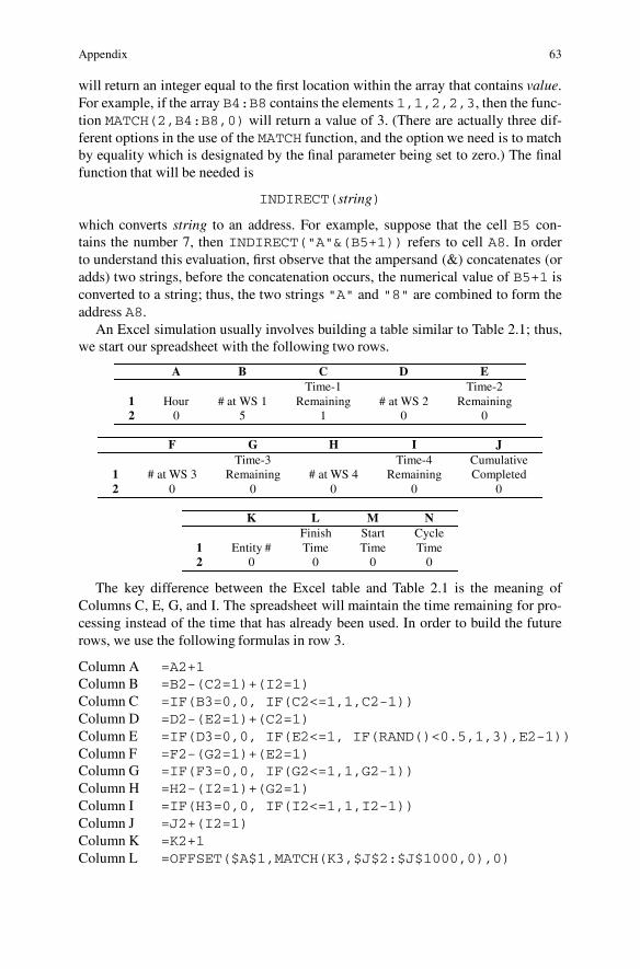
Appendix 63
will return an integer equal to the first location within the array that contains value.For example, if the array B4:B8 contains the elements 1,1,2,2,3, then the func-tion MATCH(2,B4:B8,0) will return a value of 3. (There are actually three dif-ferent options in the use of the MATCH function, and the option we need is to matchby equality which is designated by the final parameter being set to zero.) The finalfunction that will be needed is
INDIRECT(string)
which converts string to an address. For example, suppose that the cell B5 con-tains the number 7, then INDIRECT("A"&(B5+1)) refers to cell A8. In orderto understand this evaluation, first observe that the ampersand (&) concatenates (oradds) two strings, before the concatenation occurs, the numerical value of B5+1 isconverted to a string; thus, the two strings "A" and "8" are combined to form theaddress A8.
An Excel simulation usually involves building a table similar to Table 2.1; thus,we start our spreadsheet with the following two rows.
A B C D ETime-1 Time-2
1 Hour # at WS 1 Remaining # at WS 2 Remaining2 0 5 1 0 0
F G H I JTime-3 Time-4 Cumulative
1 # at WS 3 Remaining # at WS 4 Remaining Completed2 0 0 0 0 0
K L M NFinish Start Cycle
1 Entity # Time Time Time2 0 0 0 0
The key difference between the Excel table and Table 2.1 is the meaning ofColumns C, E, G, and I. The spreadsheet will maintain the time remaining for pro-cessing instead of the time that has already been used. In order to build the futurerows, we use the following formulas in row 3.
Column A =A2+1Column B =B2-(C2=1)+(I2=1)Column C =IF(B3=0,0, IF(C2<=1,1,C2-1))Column D =D2-(E2=1)+(C2=1)Column E =IF(D3=0,0, IF(E2<=1, IF(RAND()<0.5,1,3),E2-1))Column F =F2-(G2=1)+(E2=1)Column G =IF(F3=0,0, IF(G2<=1,1,G2-1))Column H =H2-(I2=1)+(G2=1)Column I =IF(H3=0,0, IF(I2<=1,1,I2-1))Column J =J2+(I2=1)Column K =K2+1Column L =OFFSET($A$1,MATCH(K3,$J$2:$J$1000,0),0)

64 2 Introduction to Factory Models
Column M =OFFSET($A$1,MATCH(K3-$B$2,$J$2:$J$1000,0),0)Column N =L3-M3
Once the formulas are entered, the range of cells A3:N1000 should be high-lighted and then the “copy down” feature (or <ctrl>-D) used to extend the tabledown. Do not be concerned that several entries in the L, M, and N columns con-tain number errors (i.e., #N/A); these are expected and should be ignored. One ofthe keys to understanding the above formulas is to recognize that a job undergoingprocessing will leave the work station whenever the time remaining at that worksta-tion equals 1. We also use the fact that when a boolean expression is used within amathematical expression, it will return the value 1 when true and return 0 whenit evaluates to false. Because the RAND function is a “volatile” function, it isrecomputed whenever the F9 key is pressed, so if you would like to see differentrealizations of the simulation, press F9.
The final step in the simulation is to report the average throughput rate (th) andthe average cycle time CT . To do this, place the word Throughput in cell P1, andput =J1000/A1000 in the P2 cell. Remember, the row 3 formulas were copieddown to row 1000; thus, the value in cell A1000 represents the total time for thesimulation and the value in cell J1000 is the total number of jobs processed throughthe simulation. In other words, theP2 cell equals the total output divided by the totaltime, which is the average throughput rate. In cell P3, place the word CycleTimeand in the P4 cell place
=AVERAGE(INDIRECT("N" & (B2+2) & ":N" & (J1000+2)))
which yields the average of the individual cycle times. To understand this formula,remember that the value of cell B2 is equal to 5 and is the initial work-in-process.The value in cell J1000 varies depending on the random outcome of the simulation.To illustrate the formula, suppose that 425 entities were processed (i.e., the valueof J1000 is 425), then the INDIRECT function will reference "N7:N427" whichcontain cycle times. (Other cells within column Nwill likely contain number errors.)The reason for using the INDIRECT function is so that when the W IP level ischanged, the CT formula will be changed to include or exclude the appropriatecells.
A final suggestion can be made with respect to the throughput rate. The rate isbiased towards the low side because the initial few hours are not representative ofsteady-state conditions. Therefore, the formula =(J1000-J48)/(A1000-A48)would give a better estimate of the long-run average value. The choice of consider-ing the first two days as comprising the transient period of operation is somewhatarbitrary and can be studied further by developing graphs of the average values if sodesired.
• Suggestion: Do Problem 2.15.
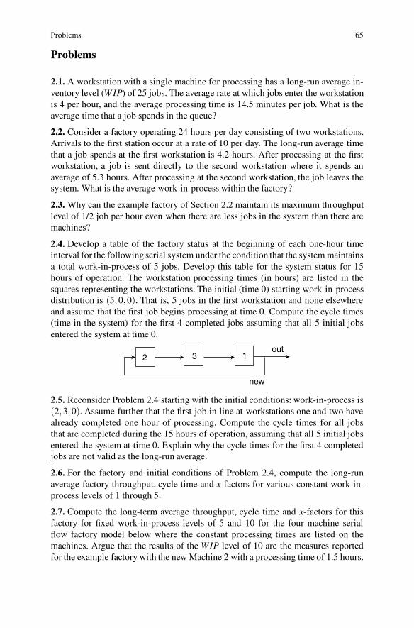
Problems 65
Problems
2.1. A workstation with a single machine for processing has a long-run average in-ventory level (W IP) of 25 jobs. The average rate at which jobs enter the workstationis 4 per hour, and the average processing time is 14.5 minutes per job. What is theaverage time that a job spends in the queue?
2.2. Consider a factory operating 24 hours per day consisting of two workstations.Arrivals to the first station occur at a rate of 10 per day. The long-run average timethat a job spends at the first workstation is 4.2 hours. After processing at the firstworkstation, a job is sent directly to the second workstation where it spends anaverage of 5.3 hours. After processing at the second workstation, the job leaves thesystem. What is the average work-in-process within the factory?
2.3. Why can the example factory of Section 2.2 maintain its maximum throughputlevel of 1/2 job per hour even when there are less jobs in the system than there aremachines?
2.4. Develop a table of the factory status at the beginning of each one-hour timeinterval for the following serial system under the condition that the system maintainsa total work-in-process of 5 jobs. Develop this table for the system status for 15hours of operation. The workstation processing times (in hours) are listed in thesquares representing the workstations. The initial (time 0) starting work-in-processdistribution is (5,0,0). That is, 5 jobs in the first workstation and none elsewhereand assume that the first job begins processing at time 0. Compute the cycle times(time in the system) for the first 4 completed jobs assuming that all 5 initial jobsentered the system at time 0.
13out
new
2
2.5. Reconsider Problem 2.4 starting with the initial conditions: work-in-process is(2,3,0). Assume further that the first job in line at workstations one and two havealready completed one hour of processing. Compute the cycle times for all jobsthat are completed during the 15 hours of operation, assuming that all 5 initial jobsentered the system at time 0. Explain why the cycle times for the first 4 completedjobs are not valid as the long-run average.
2.6. For the factory and initial conditions of Problem 2.4, compute the long-runaverage factory throughput, cycle time and x-factors for various constant work-in-process levels of 1 through 5.
2.7. Compute the long-term average throughput, cycle time and x-factors for thisfactory for fixed work-in-process levels of 5 and 10 for the four machine serialflow factory model below where the constant processing times are listed on themachines. Argue that the results of the WIP level of 10 are the measures reportedfor the example factory with the new Machine 2 with a processing time of 1.5 hours.

66 2 Introduction to Factory Models
new
out2 3 2 2
2.8. Develop a table of the factory status at the beginning of each one-hour timeinterval for the following serial system under the condition that the system maintainsa total work-in-process of 4 jobs. Develop this table for the system status for 15hours of operation. The workstation processing times (in hours) are listed in thesquares representing the workstations. The initial (time 0) starting work-in-processdistribution is (4,0,0). That is, 4 jobs in the first workstation and none elsewhereand assume the first job has yet to begin processing. Compute the cycle times (timein the system) for the first 4 completed jobs assuming that all 4 initial jobs enteredthe system at time 0.
23out
new
1
2.9. For the factory and initial conditions of Problem 2.8, compute the long-termaverage factory throughput, cycle time and x-factors for various constant WIP levels1 through 5.
2.10. Compute the long-term average throughput, cycle time and x-factors for thisfactory for fixed WIP levels of 1 through 5 for the four machine serial flow factorymodel below where the constant processing times are listed on the machines. As-sume that the factory starts with the configuration (N,0,0,0) for fixed W IP level Nand no processing has occurred on any of the active jobs.
new
out2 2 3 2
2.11. Develop a spreadsheet model to solve Problem 5.
2.12. Develop a spreadsheet model to solve Problem 6.
2.13. Develop a spreadsheet model to solve Problem 7.
2.14. Develop a spreadsheet model to solve Problem 8.
References 67
2.15. Develop a spreadsheet model of the factory in Sect. 2.2 (Fig. 2.6) except thatWorkstation 1, 2, and 4 have random processing times that are distributed accord-ing to a discrete uniform distribution between 1 and 3, and Workstation 3 has arandom processing time distributed according to a discrete uniform distributionbetween 1 and 4. To generate random integers uniformly between a and b, use"=a+FLOOR((b+1-a)*RAND(),1)".Version 2007 or Analysis Tool Pack withan earlier version of Excel provides a function to generate the discrete uniform vari-ates directly ; namely, RANDBETWEEN(a,b). (This problem is based on materialcontained in the Appendix.)
References
1. Deuermeyer, B.L., Curry, G.L., and Feldman, R.M. (1993). An Automatic Modeling Approachfor the Strategic Analysis of Manufacturing Facilities. Production and Operations Manage-ment, 2:195–220.
2. Gross, D., and Harris, C.M. (1974). Fundamentals of Queueing Theory, John Wiley & Sons,New York.
3. Hopp, W.J., and Spearman, M.L. (1996).Factory Physics: Foundationsof ManufacturingMan-agement, Irwin, Chicago.
4. Little, J.D.C. (1961). A Proof for the Queuing Formula: L = λW . Operations Research,9:383–387.
Chapter 3Single Workstation Factory Models
Throughout the analyses given in this textbook, emphasis is on the development ofsteady-state system measures such as the expected number of jobs in the system(WIP) and their mean cycle times (CT). For these analyses, it is often useful toobtain the probability mass function (pmf) of the steady-state number of jobs inthe system. From these pmf’s, the measures of system effectiveness can often bedeveloped. For notational purposes, define the random variable N as the number ofjobs in the system and define pn as the probability that the number of jobs in thesystem is n; namely, pn = Pr{N = n}. In the first section, a method is developed forderiving equations that determine the steady-state probabilities pn for n = 0,1, · · · .The initial models will include probabilistic behavior for the arrival process andprocessing times, and the early models will restrict these two probability laws to theexponential distribution.
Important assumptions on the operating characteristics of the system are alsomade. It is assumed that job inter-arrival times are independent of the status of thesystem. Another operating assumption is that the server will never be idle whenthere is a job in the system that can be served. That is, if it is allowed for the pro-cessor to serve a job, then no delay occurs between the time that one job leavesthe server and the next job begins processing on the server. Here the assumption ismade that the server is always busy processing jobs when there are jobs availablefor service. Thus, the server will only be idle when there are no jobs available. Inlater models, nonproductive times will be incorporated into the model. For example,in order to have realistic models for many systems, machine breakdowns will needto be incorporated.
3.1 First Model
Consider a single server with a limited waiting area for nmax−1 jobs and one in theserver position for a maximum of nmax jobs in the system. Jobs arrive to the systemone at a time with exponentially distributed inter-arrival times. Denoting the mean
69
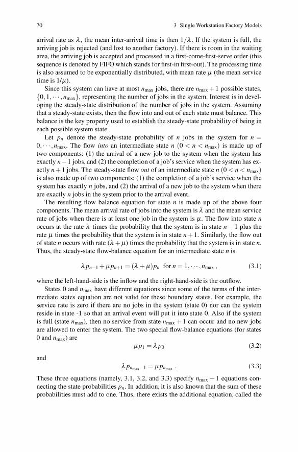
70 3 Single Workstation Factory Models
arrival rate as λ , the mean inter-arrival time is then 1/λ . If the system is full, thearriving job is rejected (and lost to another factory). If there is room in the waitingarea, the arriving job is accepted and processed in a first-come-first-serve order (thissequence is denoted by FIFO which stands for first-in first-out). The processing timeis also assumed to be exponentially distributed, with mean rate μ (the mean servicetime is 1/μ).
Since this system can have at most nmax jobs, there are nmax +1 possible states,{0,1, · · · ,nmax}, representing the number of jobs in the system. Interest is in devel-oping the steady-state distribution of the number of jobs in the system. Assumingthat a steady-state exists, then the flow into and out of each state must balance. Thisbalance is the key property used to establish the steady-state probability of being ineach possible system state.
Let pn denote the steady-state probability of n jobs in the system for n =0, · · · ,nmax. The flow into an intermediate state n (0 < n < nmax) is made up oftwo components: (1) the arrival of a new job to the system when the system hasexactly n−1 jobs, and (2) the completion of a job’s service when the system has ex-actly n +1 jobs. The steady-state flow out of an intermediate state n (0 < n < nmax)is also made up of two components: (1) the completion of a job’s service when thesystem has exactly n jobs, and (2) the arrival of a new job to the system when thereare exactly n jobs in the system prior to the arrival event.
The resulting flow balance equation for state n is made up of the above fourcomponents. The mean arrival rate of jobs into the system is λ and the mean servicerate of jobs when there is at least one job in the system is μ. The flow into state noccurs at the rate λ times the probability that the system is in state n− 1 plus therate μ times the probability that the system is in state n +1. Similarly, the flow outof state n occurs with rate (λ +μ) times the probability that the system is in state n.Thus, the steady-state flow-balance equation for an intermediate state n is
λ pn−1 + μ pn+1 = (λ + μ)pn for n = 1, · · · ,nmax , (3.1)
where the left-hand-side is the inflow and the right-hand-side is the outflow.States 0 and nmax have different equations since some of the terms of the inter-
mediate states equation are not valid for these boundary states. For example, theservice rate is zero if there are no jobs in the system (state 0) nor can the systemreside in state -1 so that an arrival event will put it into state 0. Also if the systemis full (state nmax), then no service from state nmax + 1 can occur and no new jobsare allowed to enter the system. The two special flow-balance equations (for states0 and nmax) are
μ p1 = λ p0 (3.2)
andλ pnmax−1 = μ pnmax . (3.3)
These three equations (namely, 3.1, 3.2, and 3.3) specify nmax + 1 equations con-necting the state probabilities pn. In addition, it is also known that the sum of theseprobabilities must add to one. Thus, there exists the additional equation, called the
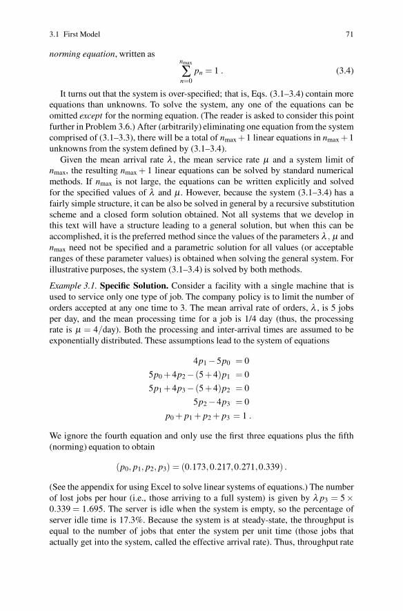
3.1 First Model 71
norming equation, written asnmax
∑n=0
pn = 1 . (3.4)
It turns out that the system is over-specified; that is, Eqs. (3.1–3.4) contain moreequations than unknowns. To solve the system, any one of the equations can beomitted except for the norming equation. (The reader is asked to consider this pointfurther in Problem 3.6.) After (arbitrarily) eliminating one equation from the systemcomprised of (3.1–3.3), there will be a total of nmax +1 linear equations in nmax +1unknowns from the system defined by (3.1–3.4).
Given the mean arrival rate λ , the mean service rate μ and a system limit ofnmax, the resulting nmax + 1 linear equations can be solved by standard numericalmethods. If nmax is not large, the equations can be written explicitly and solvedfor the specified values of λ and μ. However, because the system (3.1–3.4) has afairly simple structure, it can be also be solved in general by a recursive substitutionscheme and a closed form solution obtained. Not all systems that we develop inthis text will have a structure leading to a general solution, but when this can beaccomplished, it is the preferred method since the values of the parameters λ , μ andnmax need not be specified and a parametric solution for all values (or acceptableranges of these parameter values) is obtained when solving the general system. Forillustrative purposes, the system (3.1–3.4) is solved by both methods.
Example 3.1. Specific Solution. Consider a facility with a single machine that isused to service only one type of job. The company policy is to limit the number oforders accepted at any one time to 3. The mean arrival rate of orders, λ , is 5 jobsper day, and the mean processing time for a job is 1/4 day (thus, the processingrate is μ = 4/day). Both the processing and inter-arrival times are assumed to beexponentially distributed. These assumptions lead to the system of equations
4p1 −5p0 = 0
5p0 +4p2 − (5 +4)p1 = 0
5p1 +4p3 − (5 +4)p2 = 0
5p2 −4p3 = 0
p0 + p1 + p2 + p3 = 1 .
We ignore the fourth equation and only use the first three equations plus the fifth(norming) equation to obtain
(p0, p1, p2, p3) = (0.173,0.217,0.271,0.339) .
(See the appendix for using Excel to solve linear systems of equations.) The numberof lost jobs per hour (i.e., those arriving to a full system) is given by λ p3 = 5×0.339 = 1.695. The server is idle when the system is empty, so the percentage ofserver idle time is 17.3%. Because the system is at steady-state, the throughput isequal to the number of jobs that enter the system per unit time (those jobs thatactually get into the system, called the effective arrival rate). Thus, throughput rate
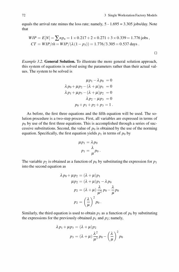
72 3 Single Workstation Factory Models
equals the arrival rate minus the loss rate; namely, 5 - 1.695 = 3.305 jobs/day. Notethat
WIP = E[N] = ∑npn = 1×0.217 +2×0.271 +3×0.339 = 1.776 jobs ,
CT = W IP/th = W IP/(λ (1− p3)) = 1.776/3.305 = 0.537 days .
��
Example 3.2. General Solution. To illustrate the more general solution approach,this system of equations is solved using the parameters rather than their actual val-ues. The system to be solved is
μ p1 −λ p0 = 0
λ p0 + μ p2 − (λ + μ)p1 = 0
λ p1 + μ p3 − (λ + μ)p2 = 0
λ p2 −μ p3 = 0
p0 + p1 + p2 + p3 = 1 .
As before, the first three equations and the fifth equation will be used. The so-lution procedure is a two-step process. First, all variables are expressed in terms ofp0 by use of the first three equations. This is accomplished through a series of suc-cessive substitutions. Second, the value of p0 is obtained by the use of the normingequation. Specifically, the first equation yields p1 in terms of p0 by
μ p1 = λ p0
p1 =λμ
p0 .
The variable p2 is obtained as a function of p0 by substituting the expression for p1
into the second equation as
λ p0 + μ p2 = (λ + μ)p1
μ p2 = (λ + μ)p1 −λ p0
p2 = (λ + μ)λμ2 p0 −
λμ
p0
p2 =(
λμ
)2
p0 .
Similarly, the third equation is used to obtain p3 as a function of p0 by substitutingthe expressions for the previously obtained p1 and p2; namely,
λ p1 + μ p3 = (λ + μ)p2
p3 = (λ + μ)λ 2
μ3 p0 −(
λμ
)2
p0
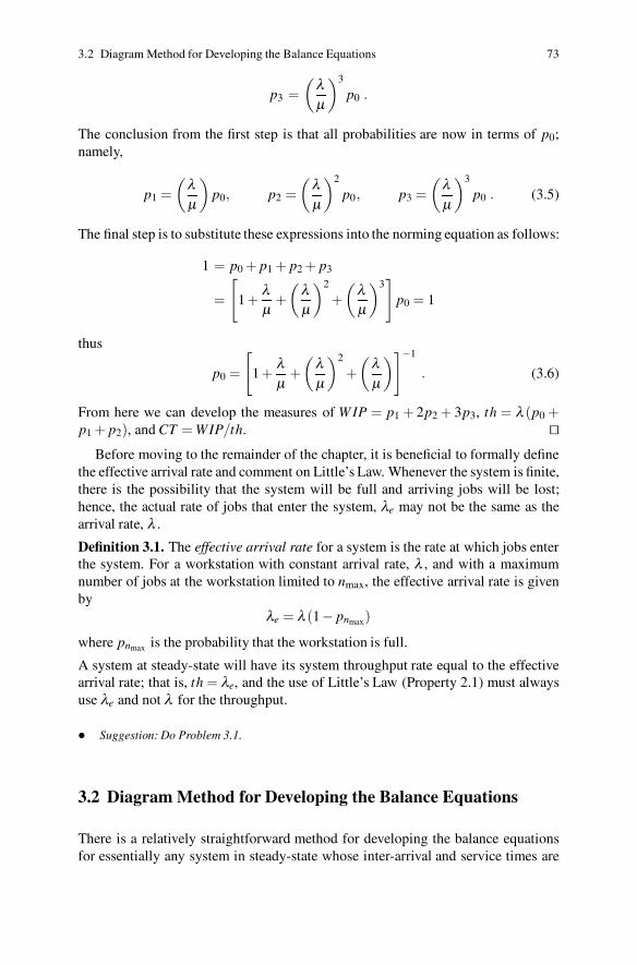
3.2 Diagram Method for Developing the Balance Equations 73
p3 =(
λμ
)3
p0 .
The conclusion from the first step is that all probabilities are now in terms of p0;namely,
p1 =(
λμ
)
p0, p2 =(
λμ
)2
p0, p3 =(
λμ
)3
p0 . (3.5)
The final step is to substitute these expressions into the norming equation as follows:
1 = p0 + p1 + p2 + p3
=
[
1 +λμ
+(
λμ
)2
+(
λμ
)3]
p0 = 1
thus
p0 =
[
1 +λμ
+(
λμ
)2
+(
λμ
)
]−1
. (3.6)
From here we can develop the measures of W IP = p1 + 2p2 + 3p3, th = λ (p0 +p1 + p2), and CT = WIP/th. ��
Before moving to the remainder of the chapter, it is beneficial to formally definethe effective arrival rate and comment on Little’s Law. Whenever the system is finite,there is the possibility that the system will be full and arriving jobs will be lost;hence, the actual rate of jobs that enter the system, λe may not be the same as thearrival rate, λ .
Definition 3.1. The effective arrival rate for a system is the rate at which jobs enterthe system. For a workstation with constant arrival rate, λ , and with a maximumnumber of jobs at the workstation limited to nmax, the effective arrival rate is givenby
λe = λ (1− pnmax)
where pnmax is the probability that the workstation is full.
A system at steady-state will have its system throughput rate equal to the effectivearrival rate; that is, th = λe, and the use of Little’s Law (Property 2.1) must alwaysuse λe and not λ for the throughput.
• Suggestion: Do Problem 3.1.
3.2 Diagram Method for Developing the Balance Equations
There is a relatively straightforward method for developing the balance equationsfor essentially any system in steady-state whose inter-arrival and service times are
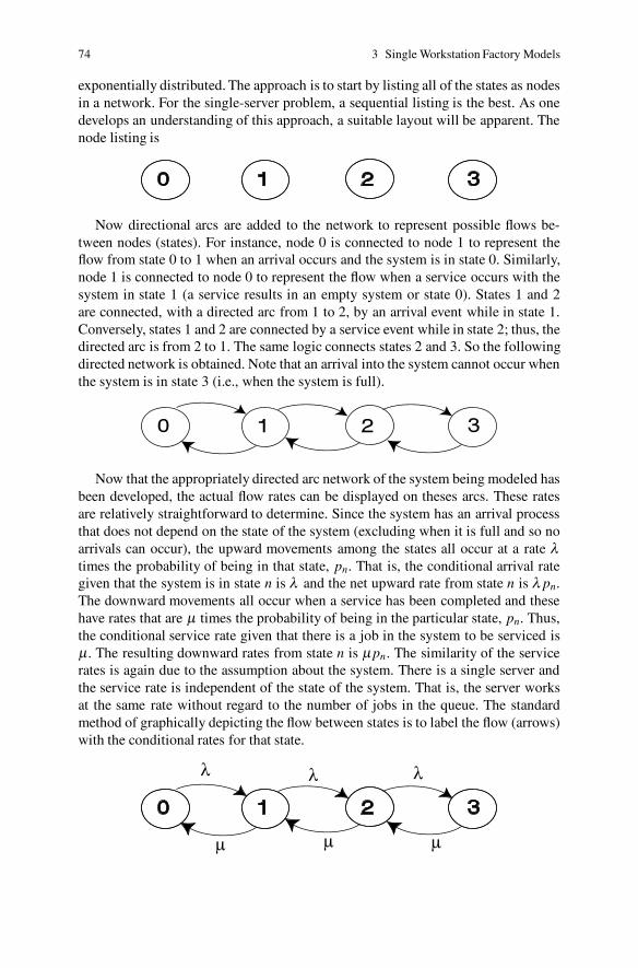
74 3 Single Workstation Factory Models
exponentially distributed. The approach is to start by listing all of the states as nodesin a network. For the single-server problem, a sequential listing is the best. As onedevelops an understanding of this approach, a suitable layout will be apparent. Thenode listing is
Now directional arcs are added to the network to represent possible flows be-tween nodes (states). For instance, node 0 is connected to node 1 to represent theflow from state 0 to 1 when an arrival occurs and the system is in state 0. Similarly,node 1 is connected to node 0 to represent the flow when a service occurs with thesystem in state 1 (a service results in an empty system or state 0). States 1 and 2are connected, with a directed arc from 1 to 2, by an arrival event while in state 1.Conversely, states 1 and 2 are connected by a service event while in state 2; thus, thedirected arc is from 2 to 1. The same logic connects states 2 and 3. So the followingdirected network is obtained. Note that an arrival into the system cannot occur whenthe system is in state 3 (i.e., when the system is full).
Now that the appropriately directed arc network of the system being modeled hasbeen developed, the actual flow rates can be displayed on theses arcs. These ratesare relatively straightforward to determine. Since the system has an arrival processthat does not depend on the state of the system (excluding when it is full and so noarrivals can occur), the upward movements among the states all occur at a rate λtimes the probability of being in that state, pn. That is, the conditional arrival rategiven that the system is in state n is λ and the net upward rate from state n is λ pn.The downward movements all occur when a service has been completed and thesehave rates that are μ times the probability of being in the particular state, pn. Thus,the conditional service rate given that there is a job in the system to be serviced isμ. The resulting downward rates from state n is μ pn. The similarity of the servicerates is again due to the assumption about the system. There is a single server andthe service rate is independent of the state of the system. That is, the server worksat the same rate without regard to the number of jobs in the queue. The standardmethod of graphically depicting the flow between states is to label the flow (arrows)with the conditional rates for that state.
μ
λ λ λ
μ μ
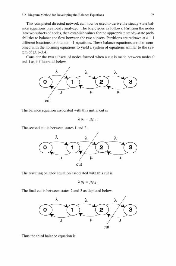
3.2 Diagram Method for Developing the Balance Equations 75
This completed directed network can now be used to derive the steady-state bal-ance equations previously analyzed. The logic goes as follows. Partition the nodesinto two subsets of nodes, then establish values for the appropriate steady-state prob-abilities to balance the flow between the two subsets. Partitions are redrawn at n−1different locations to obtain n−1 equations. These balance equations are then com-bined with the norming equations to yield a system of equations similar to the sys-tem of (3.1–3.4).
Consider the two subsets of nodes formed when a cut is made between nodes 0and 1 as is illustrated below.
μ μ
λ λ λ
cut
μ
The balance equation associated with this initial cut is
λ p0 = μ p1 .
The second cut is between states 1 and 2.
μ μ μ
λ λ λ
cut
The resulting balance equation associated with this cut is
λ p1 = μ p2 .
The final cut is between states 2 and 3 as depicted below.
μ μ μ
λ λ λ
cut
Thus the third balance equation is
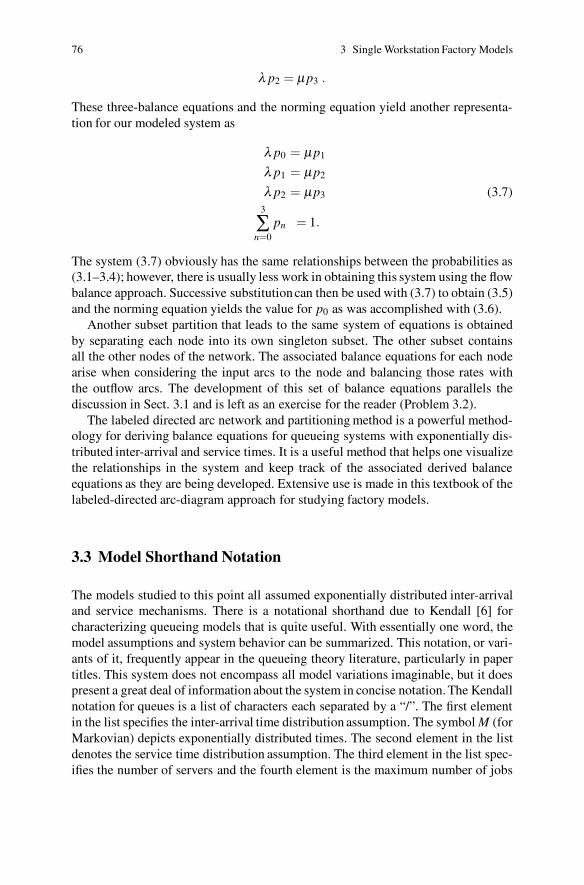
76 3 Single Workstation Factory Models
λ p2 = μ p3 .
These three-balance equations and the norming equation yield another representa-tion for our modeled system as
λ p0 = μ p1
λ p1 = μ p2
λ p2 = μ p3 (3.7)3
∑n=0
pn = 1.
The system (3.7) obviously has the same relationships between the probabilities as(3.1–3.4); however, there is usually less work in obtaining this system using the flowbalance approach. Successive substitution can then be used with (3.7) to obtain (3.5)and the norming equation yields the value for p0 as was accomplished with (3.6).
Another subset partition that leads to the same system of equations is obtainedby separating each node into its own singleton subset. The other subset containsall the other nodes of the network. The associated balance equations for each nodearise when considering the input arcs to the node and balancing those rates withthe outflow arcs. The development of this set of balance equations parallels thediscussion in Sect. 3.1 and is left as an exercise for the reader (Problem 3.2).
The labeled directed arc network and partitioning method is a powerful method-ology for deriving balance equations for queueing systems with exponentially dis-tributed inter-arrival and service times. It is a useful method that helps one visualizethe relationships in the system and keep track of the associated derived balanceequations as they are being developed. Extensive use is made in this textbook of thelabeled-directed arc-diagram approach for studying factory models.
3.3 Model Shorthand Notation
The models studied to this point all assumed exponentially distributed inter-arrivaland service mechanisms. There is a notational shorthand due to Kendall [6] forcharacterizing queueing models that is quite useful. With essentially one word, themodel assumptions and system behavior can be summarized. This notation, or vari-ants of it, frequently appear in the queueing theory literature, particularly in papertitles. This system does not encompass all model variations imaginable, but it doespresent a great deal of information about the system in concise notation. The Kendallnotation for queues is a list of characters each separated by a “/”. The first elementin the list specifies the inter-arrival time distribution assumption. The symbol M (forMarkovian) depicts exponentially distributed times. The second element in the listdenotes the service time distribution assumption. The third element in the list spec-ifies the number of servers and the fourth element is the maximum number of jobs
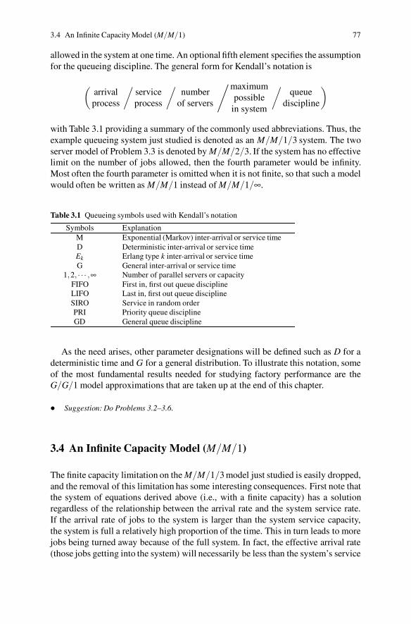
3.4 An Infinite Capacity Model (M/M/1) 77
allowed in the system at one time. An optional fifth element specifies the assumptionfor the queueing discipline. The general form for Kendall’s notation is
(
arrivalprocess
/
serviceprocess
/
numberof servers
/maximumpossible
in system
/
queuediscipline
)
with Table 3.1 providing a summary of the commonly used abbreviations. Thus, theexample queueing system just studied is denoted as an M/M/1/3 system. The twoserver model of Problem 3.3 is denoted by M/M/2/3. If the system has no effectivelimit on the number of jobs allowed, then the fourth parameter would be infinity.Most often the fourth parameter is omitted when it is not finite, so that such a modelwould often be written as M/M/1 instead of M/M/1/∞.
Table 3.1 Queueing symbols used with Kendall’s notation
Symbols ExplanationM Exponential (Markov) inter-arrival or service timeD Deterministic inter-arrival or service timeEk Erlang type k inter-arrival or service timeG General inter-arrival or service time
1,2, · · · ,∞ Number of parallel servers or capacityFIFO First in, first out queue disciplineLIFO Last in, first out queue disciplineSIRO Service in random orderPRI Priority queue disciplineGD General queue discipline
As the need arises, other parameter designations will be defined such as D for adeterministic time and G for a general distribution. To illustrate this notation, someof the most fundamental results needed for studying factory performance are theG/G/1 model approximations that are taken up at the end of this chapter.
• Suggestion: Do Problems 3.2–3.6.
3.4 An Infinite Capacity Model (M/M/1)
The finite capacity limitation on the M/M/1/3 model just studied is easily dropped,and the removal of this limitation has some interesting consequences. First note thatthe system of equations derived above (i.e., with a finite capacity) has a solutionregardless of the relationship between the arrival rate and the system service rate.If the arrival rate of jobs to the system is larger than the system service capacity,the system is full a relatively high proportion of the time. This in turn leads to morejobs being turned away because of the full system. In fact, the effective arrival rate(those jobs getting into the system) will necessarily be less than the system’s service

78 3 Single Workstation Factory Models
capacity. Let’s consider a few cases for the above example that illustrate this point.Suppose that the mean arrival rate is equal to the mean service rate, λ = μ for theM/M/1/3 system. With λ = μ, each probability is equal so that p0 = · · ·= p3 =1/4. The effective arrival rate is, thus, given by λe = λ (1− p3) = (3/4)λ < μ. If themean arrival rate is twice the mean service rate, λ = 2μ, then the effective arrivalrate becomes λe = (7/15)λ < μ. For a mean arrival rate that is three times themean service rate, λ = 3μ, the effective arrival rate becomes λe = (13/40)λ < μ.Note that as the ratio of λ/μ becomes larger, the effective arrival rate approachesthe inverse of this ratio but never reaches it. The reader is asked to compute theseeffective rates in Problem 3.5.
One of the lessons to be learned from the finite capacity model is that these sys-tems have a built-in mechanism to adjust the arrival rate (called the effective arrivalrate) to a level that can be handled by the system service capacity. If a system that hasno realistic limit on the number of jobs allowed is considered, then mathematically,these systems can be put in a situation where the mean arrival rate exceeds the meanservice rate and no steady-state exists. It is unreasonable to assume that jobs con-tinue to arrive when there is essentially an infinite queue and the expected cycle timeis also infinite. Of course, one would like to operate well below the blowup pointwith respect to the arrival and service capacity ratio. The analyses of the unlimitedqueueing models result in conditions that establish the existence of the steady-statebehavior for these models.
The formulation of the unlimited-jobs system is very analogous to the finite ca-pacity model formulation. The solution procedure is considerably different in thatan infinite number of states exist and, correspondingly, an infinite number of de-scriptive equations result. Thus, standard numerical solutions for linear equationscannot be used. One is forced to solve these systems in a fashion analogous to theparametric solution approach illustrated for the finite capacity systems. This methodis essentially substitution and formulation of a recursive relationship for the generalsolution structure.
The set of equations for the M/M/1 system is the same as the equations for thefinite system capacity case except that the system does not have a final equation.Thus, an infinite system of equations exists. The diagram for this system is depictedbelow.
21 30 ...
Using the cut partitioning method for obtaining the system of equations neededin defining the steady-state probabilities, the following is obtained:
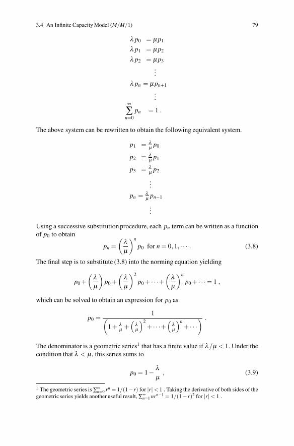
3.4 An Infinite Capacity Model (M/M/1) 79
λ p0 = μ p1
λ p1 = μ p2
λ p2 = μ p3
...
λ pn = μ pn+1
...∞
∑n=0
pn = 1 .
The above system can be rewritten to obtain the following equivalent system.
p1 = λμ p0
p2 = λμ p1
p3 = λμ p2
...
pn = λμ pn−1
...
Using a successive substitution procedure, each pn term can be written as a functionof p0 to obtain
pn =(
λμ
)n
p0 for n = 0,1, · · · . (3.8)
The final step is to substitute (3.8) into the norming equation yielding
p0 +(
λμ
)
p0 +(
λμ
)2
p0 + · · ·+(
λμ
)n
p0 + · · ·= 1 ,
which can be solved to obtain an expression for p0 as
p0 =1
(
1 + λμ +(
λμ
)2+ · · ·+
(
λμ
)n+ · · ·
) .
The denominator is a geometric series1 that has a finite value if λ/μ < 1. Under thecondition that λ < μ, this series sums to
p0 = 1− λμ
, (3.9)
1 The geometric series is ∑∞n=0 rn = 1/(1−r) for |r|< 1 . Taking the derivative of both sides of the
geometric series yields another useful result, ∑∞n=1 nrn−1 = 1/(1− r)2 for |r|< 1 .

80 3 Single Workstation Factory Models
and the general solution to the steady-state probabilities is (given that λ/μ < 1)
pn =(
1− λμ
)(
λμ
)n
for n = 0,1, · · · . (3.10)
The throughput rate per unit time for this system is λ . (The reader is asked to de-velop this result in Problem 3.10.) The utilization factor u for the server is obtainedfrom
u = 0p0 +1
(
∞
∑n=1
pn
)
= 1− p0 = 1−(
1− λμ
)
=λμ
.
The expected number of jobs in the system in steady-state is obtained by using thederivative of the geometric series as follows:
W IPs = E[N] =∞
∑n=0
npn =∞
∑n=0
n
(
1− λμ
)(
λμ
)n
=(
1− λμ
)(
λμ
) ∞
∑n=1
n
(
λμ
)n−1
=(
1− λμ
)(
λμ
)
(
1
1− λμ
)2
=
(
1− λμ
)(
λμ
)
(
1− λμ
)2 =λμ
(
1− λμ
) =u
1−u(3.11)
where N is a random variable denoting the number of jobs in the system. UsingLittle’s Law (Property 2.1), the expected time in system (the cycle time) CTs isgiven by
CTs =W IPs
λ=
1λ
λμ
(1− λμ )
=1
μ −λ. (3.12)
Example 3.3. Consider a single server system with exponentially-distributed inter-arrival times and exponentially-distributed service times (thus, this is an M/M/1system). If 4 jobs per hour arrive for service (λ = 4) and the mean service time is1/5 hour (μ = 5), then the utilization factor u (u = λ/μ) equals 0.8. The expectednumber of jobs in the system, W IPs from (3.11) is
W IPs =0.8
(1−0.8)= 4 .
The cycle time in the system, CTs, is given by (3.12) and is
CTs =1
5−4= 1 hr .

3.5 Multiple Server Systems with Non-identical Service Rates 81
The cycle time in the system is the sum of the cycle time in the queue plus theservice time. Hence, CTq = 1−0.2 = 0.8 hr. The probability that the server is idle,of course, equals the probability that the system is empty, p0. This probability is
p0 = 1− λμ
= 0.2 .
The steady-state probability that there are n jobs in the system is given by
pn = 0.2×0.8n for n = 0,1, · · · .
��
A workstation may consist of multiple machines; however, in most models,server or machine distinctions are not usually made. That is, if there are two ma-chines available, then for ease of modeling it is usually assumed that these are iden-tical machines and that jobs are not split, but processed completely on one machine.Under the assumption of identical machines, if one machine operates at a rate ofμ, then n machines operate at a rate of nμ, and the state diagram must be adjustedaccordingly. For example, suppose a workstation has three machines, then the ser-vice rate when two machines are busy is 2μ and whenever all machines are busy theservice rate is 3μ; thus, the rate diagram is as below.
21 30 ...
μ 2μ 3μ 3μ
• Suggestion: Do Problems 3.7–3.14.
3.5 Multiple Server Systems with Non-identical Service Rates
The assumptions of identical machines may not be accurate, and if there is a sig-nificant difference in the operating characteristics of the machines associated with asingle workstation, more complex models will result. To provide some exposure tothe complexity involved in modeling non-identical machines within a single work-station, a simple non-identical servers model is considered and the associated defin-ing equations for the steady-state probabilities are developed. The structure of thissystem is that it has two non-identical servers and a limit of four jobs in the sys-tem at one time. Inter-arrival and service times are all assumed to be exponentiallydistributed with a mean arrival rate of λ and mean service rates of μ and γ for thetwo distinct machines. Let γ < μ, so that the μ machine is faster and, therefore,
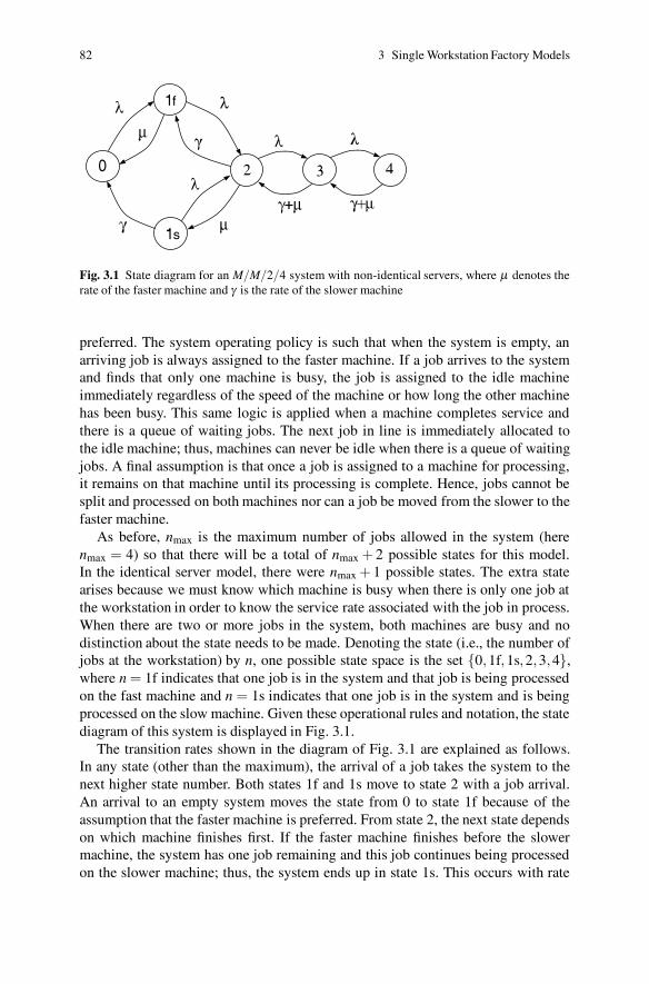
82 3 Single Workstation Factory Models
s
f
Fig. 3.1 State diagram for an M/M/2/4 system with non-identical servers, where μ denotes therate of the faster machine and γ is the rate of the slower machine
preferred. The system operating policy is such that when the system is empty, anarriving job is always assigned to the faster machine. If a job arrives to the systemand finds that only one machine is busy, the job is assigned to the idle machineimmediately regardless of the speed of the machine or how long the other machinehas been busy. This same logic is applied when a machine completes service andthere is a queue of waiting jobs. The next job in line is immediately allocated tothe idle machine; thus, machines can never be idle when there is a queue of waitingjobs. A final assumption is that once a job is assigned to a machine for processing,it remains on that machine until its processing is complete. Hence, jobs cannot besplit and processed on both machines nor can a job be moved from the slower to thefaster machine.
As before, nmax is the maximum number of jobs allowed in the system (herenmax = 4) so that there will be a total of nmax + 2 possible states for this model.In the identical server model, there were nmax + 1 possible states. The extra statearises because we must know which machine is busy when there is only one job atthe workstation in order to know the service rate associated with the job in process.When there are two or more jobs in the system, both machines are busy and nodistinction about the state needs to be made. Denoting the state (i.e., the number ofjobs at the workstation) by n, one possible state space is the set {0,1f,1s,2,3,4},where n = 1f indicates that one job is in the system and that job is being processedon the fast machine and n = 1s indicates that one job is in the system and is beingprocessed on the slow machine. Given these operational rules and notation, the statediagram of this system is displayed in Fig. 3.1.
The transition rates shown in the diagram of Fig. 3.1 are explained as follows.In any state (other than the maximum), the arrival of a job takes the system to thenext higher state number. Both states 1f and 1s move to state 2 with a job arrival.An arrival to an empty system moves the state from 0 to state 1f because of theassumption that the faster machine is preferred. From state 2, the next state dependson which machine finishes first. If the faster machine finishes before the slowermachine, the system has one job remaining and this job continues being processedon the slower machine; thus, the system ends up in state 1s. This occurs with rate
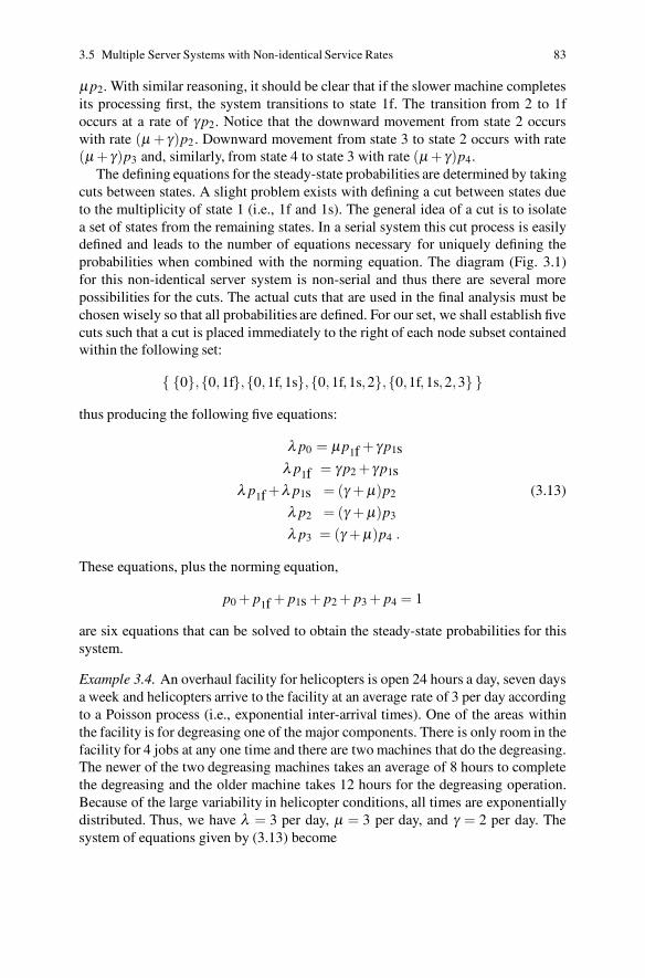
3.5 Multiple Server Systems with Non-identical Service Rates 83
μ p2. With similar reasoning, it should be clear that if the slower machine completesits processing first, the system transitions to state 1f. The transition from 2 to 1foccurs at a rate of γ p2. Notice that the downward movement from state 2 occurswith rate (μ + γ)p2. Downward movement from state 3 to state 2 occurs with rate(μ + γ)p3 and, similarly, from state 4 to state 3 with rate (μ + γ)p4.
The defining equations for the steady-state probabilities are determined by takingcuts between states. A slight problem exists with defining a cut between states dueto the multiplicity of state 1 (i.e., 1f and 1s). The general idea of a cut is to isolatea set of states from the remaining states. In a serial system this cut process is easilydefined and leads to the number of equations necessary for uniquely defining theprobabilities when combined with the norming equation. The diagram (Fig. 3.1)for this non-identical server system is non-serial and thus there are several morepossibilities for the cuts. The actual cuts that are used in the final analysis must bechosen wisely so that all probabilities are defined. For our set, we shall establish fivecuts such that a cut is placed immediately to the right of each node subset containedwithin the following set:
{ {0},{0,1f},{0,1f,1s},{0,1f,1s,2},{0,1f,1s,2,3} }
thus producing the following five equations:
λ p0 = μ p1f + γ p1sλ p1f = γ p2 + γ p1s
λ p1f +λ p1s = (γ + μ)p2 (3.13)
λ p2 = (γ + μ)p3
λ p3 = (γ + μ)p4 .
These equations, plus the norming equation,
p0 + p1f + p1s + p2 + p3 + p4 = 1
are six equations that can be solved to obtain the steady-state probabilities for thissystem.
Example 3.4. An overhaul facility for helicopters is open 24 hours a day, seven daysa week and helicopters arrive to the facility at an average rate of 3 per day accordingto a Poisson process (i.e., exponential inter-arrival times). One of the areas withinthe facility is for degreasing one of the major components. There is only room in thefacility for 4 jobs at any one time and there are two machines that do the degreasing.The newer of the two degreasing machines takes an average of 8 hours to completethe degreasing and the older machine takes 12 hours for the degreasing operation.Because of the large variability in helicopter conditions, all times are exponentiallydistributed. Thus, we have λ = 3 per day, μ = 3 per day, and γ = 2 per day. Thesystem of equations given by (3.13) become
84 3 Single Workstation Factory Models
3p0 −3p1f−2p1s = 0
3p1f−2p2 −2p1s = 0
3p1f +3p1s −5p2 = 0
3p2−5p3 = 0
3p3−5p4 = 0
p0 + p1f + p1s + p2 + p3 + p4 = 1 .
The solution to this system of equations is
p0 = 0.288, p1f = 0.209, p1s = 0.118, p2 = 0.196, p3 = 0.118, p4 = 0.071 .
The average number in the system is obtained by using the definition of an ex-pected value; namely,
WIPs = p1f + p1s +2p2 +3p3 +4p4 = 1.356
and the average number in the queue is obtained similarly,
W IPq = p3 +2p4 = 0.259 .
Note that for the average number in the queue, p3 is multiplied by 1 because whenthere are 3 in the system, there is only 1 in the queue. Also, p4 is multiplied by2 because when there are 4 in the system, there are 2 in the queue. Average cycletimes are obtained through Little’s Law as
CTs =W IPs
λe=
1.3563× (1−0.071)
= 0.486 day
CTq =W IPq
λe=
0.2593× (1−0.071)
= 0.093 day .
A couple of other measures that are sometimes desired by management are thenumber of busy processors (i.e., degreasers) and their utilization. The expected num-ber of busy servers, E[BS], is 1.097, and is obtained as
E[BS] = 1p1f +1p1s +2p2 +2P3 +2p4 = 1.097 .
The system utilization factor u is the expected number of busy servers divided bythe number of machines available
u =E[BS]
2= 0.5485 = 54.85% .
Our final calculation is to obtain the average time needed for degreasing. Be-cause of the preference given to using the faster machine, we would expect theaverage time to be closer to 8 hours than to 12 hours. To get an exact value, we takeadvantage of the fact that the time in the system equals the time in the queue plus
3.6 Using Exponentials to Approximate General Times 85
service time (Eq. 2.1); thus
E[T ] = CTs −CTq = 0.486−0.093 = 0.393 days = 9.4 hr .
��
• Suggestion: Do Problems 3.15–3.20.
3.6 Using Exponentials to Approximate General Times
The exponential distribution is an extremely powerful modeling tool because of itslack of memory (Eq. 1.16 and Problem 1.24). That is, the rate of completion of theprocess does not change with elapsed time. So for systems with exponential times,it is not necessary to keep track of the elapsed inter-arrival time nor the elapsedservice time. This allows the steady-state modeling approach to be used. To modelmore general systems, one fruitful approach is to approximate the general times bycombinations of exponentials. Then the exponential rate modeling approach can stillbe applied by developing more complex state representations of the system.
The Erlang-k distribution (see p. 18 for a review of the Erlang) provides an ex-cellent distribution to use for the expanded state modeling approach. The Erlang-kdistribution is the sum of k independent and identical exponential distributions, sothat it can be modeled as a serial k-node system, with each node referring to iden-tical exponentials. Since the Erlang-k has a squared coefficient of variation givenby C2 = 1/k, it also allows modeling of processes that have less variation than theexponential distribution.
3.6.1 Erlang Processing Times
To illustrate the expanded state modeling approach, consider a single server sys-tem with exponential inter-arrival times having a mean rate λ and a processing timethat is described by an Erlang-2 distribution with mean rate μ and thus mean time1/μ. This Erlang-2 distribution will be modeled using two exponential nodes (orphases), where each node has a mean rate of 2μ. Since rates and times are recipro-cals, the mean time spent in each node is 1/(2μ). This gives the total time spent inthe two nodes as 1/μ (i.e., the sum of the two means) which is equal to the averagetime of the Erlang-2 processing time distribution. To further simplify this example,the number of jobs allowed into the system will be limited to three. Thus, we areinterested in analyzing an M/E2/1/3 system.
The idea of the expanded state space approach is to represent the non-exponentialprocess by more that one node, where each individual node is exponential. There-fore, the service process will have two nodes representing the two phases of theErlang-2 distribution. When a job begins its processing, it enters the node represent-
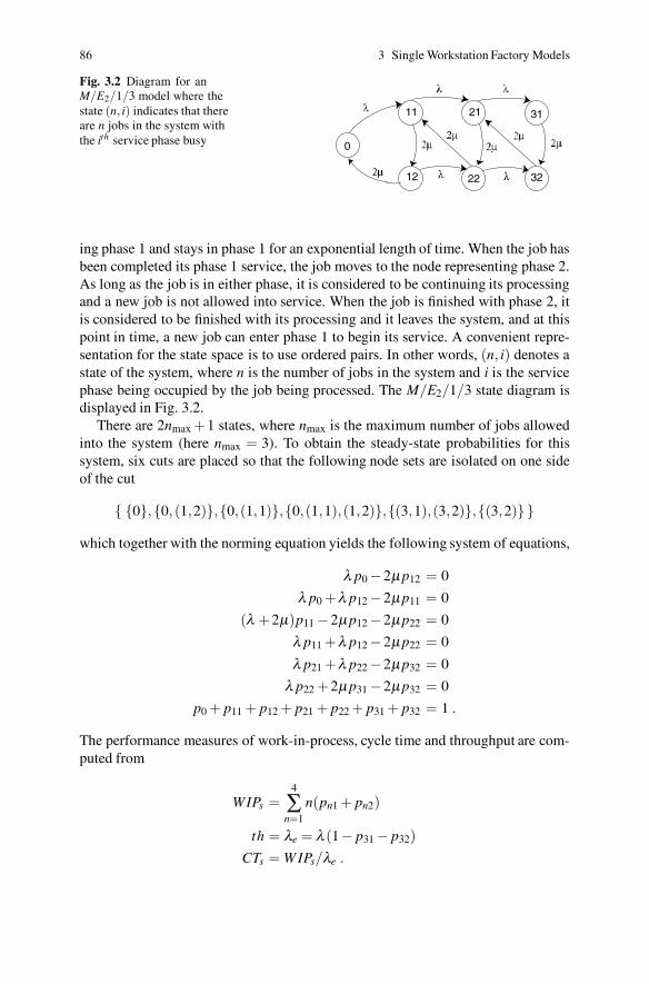
86 3 Single Workstation Factory Models
Fig. 3.2 Diagram for anM/E2/1/3 model where thestate (n, i) indicates that thereare n jobs in the system withthe ith service phase busy
11
12
31
0
21
22 32
ing phase 1 and stays in phase 1 for an exponential length of time. When the job hasbeen completed its phase 1 service, the job moves to the node representing phase 2.As long as the job is in either phase, it is considered to be continuing its processingand a new job is not allowed into service. When the job is finished with phase 2, itis considered to be finished with its processing and it leaves the system, and at thispoint in time, a new job can enter phase 1 to begin its service. A convenient repre-sentation for the state space is to use ordered pairs. In other words, (n, i) denotes astate of the system, where n is the number of jobs in the system and i is the servicephase being occupied by the job being processed. The M/E2/1/3 state diagram isdisplayed in Fig. 3.2.
There are 2nmax +1 states, where nmax is the maximum number of jobs allowedinto the system (here nmax = 3). To obtain the steady-state probabilities for thissystem, six cuts are placed so that the following node sets are isolated on one sideof the cut
{ {0},{0, (1,2)},{0,(1,1)},{0,(1,1),(1,2)},{(3,1),(3,2)},{(3,2)} }
which together with the norming equation yields the following system of equations,
λ p0 −2μ p12 = 0
λ p0 +λ p12 −2μ p11 = 0
(λ +2μ)p11 −2μ p12 −2μ p22 = 0
λ p11 +λ p12 −2μ p22 = 0
λ p21 +λ p22 −2μ p32 = 0
λ p22 +2μ p31 −2μ p32 = 0
p0 + p11 + p12 + p21 + p22 + p31 + p32 = 1 .
The performance measures of work-in-process, cycle time and throughput are com-puted from
WIPs =4
∑n=1
n(pn1 + pn2)
th = λe = λ (1− p31 − p32)CTs = W IPs/λe .
3.6 Using Exponentials to Approximate General Times 87
3.6.2 Erlang Inter-Arrival Times
If the inter-arrival process is an Erlang distribution then the state-space scheme isslightly different from that used for Erlang service. The same concept of breakingthe service process into phases is used for the arrival process; however, the statespace will be slightly different. We illustrate the expanded state space process ap-plied to arrivals by assuming an Erlang-2 inter-arrival time process. The arrivals willbe processed one-at-a-time at a single workstation with exponentially distributedservice times with a limit of three jobs in the system, in other words, we consider anE2/M/1/3 system.
Conceptually, an arriving job is always in one of two phases, and each phase hasa mean rate of 2λ or a mean sojourn time of 1/(2λ ). As long as a job is in one ofthe arrival phases, it is not yet considered part of the system. The arriving job beginsin phase 1. After an exponentially distributed length of time, the job transitions tophase 2. After another exponential length of time, two events occur simultaneously:the job leaves phase 2 and enters the system and another jobs enters phase 1. (Notethat for a model of phased arrivals, one of the arrival phases is always occupied andthe other phases are empty.)
The slight difference in the state space for the Erlang inter-arrival time modelversus the Erlang service time model occurs due to the situation that the arrivalprocess has two phases regardless of the number of jobs in the system. So when thesystem is empty, there are still two phases that the arriving job must complete beforeit becomes an active job attempting to enter the system. The state-space notationused is (i,n) where as before i is the phase and n is the number of jobs in thesystem. Note that the order has been reversed from the Erlang service model to helpkeep in mind that the phases are for the arrival process. The states needed to modelthe E2/M/1/3 system are: {(1,0), (2,0), (1,1), (2,1), (1,2), (2,2), (1,3), (2,3)}. Thediagram of this model is given in Fig. 3.3. Note also that there is a different situationfor blocked jobs for this model. A job is not blocked until it arrives to a full systemwhich occurs from state (2,3) with rate 2λ . Then the arrival process starts over instate (1,3) rather than staying at state (2,3). That is, the arriving job is rejected andthe arrival process starts over at state (1,3) for the next job creation. Thus, there isan arc between (2,3) and (1,3) with rate 2λ in Fig. 3.3 to represent this transition.
Instead of using cuts to derive the equations of state, we use the single-node iso-lation method for generating the equations that define the steady-state probabilities.The following system of equations (all eight equations are given but only seven areused since the norming equation is also required) are generated for the states in theorder that they appear in the above state list.
2λ p10 = μ p11
2λ p20 = 2λ p10 + μ p21
(2λ + μ)p11 = 2λ p20 + μ p12
(2λ + μ)p21 = 2λ p11 + μ p22
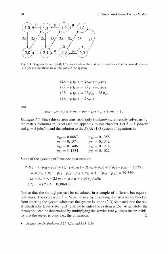
88 3 Single Workstation Factory Models
1,0μ μ μ
μμ μ
1,1 1,2 1,3
2,0 2,1 2,2 2,3
2λ 2λ 2λ 2λ 2λ 2λ 2λ 2λ
Fig. 3.3 Diagram for an E2/M/1/3 model where the state (i,n) indicates that the arrival processis in phase i and there are n total jobs in the system
(2λ + μ)p12 = 2λ p21 + μ p13
(2λ + μ)p22 = 2λ p12 + μ p23
(2λ + μ)p13 = 2λ p22 +2λ p23
(2λ + μ)p23 = 2λ p13
andp10 + p20 + p11 + p21 + p12 + p22 + p13 + p23 = 1 .
Example 3.5. Since this system consists of only 8 unknowns, it is easily solved usingthe matrix formulas in Excel (see the appendix to this chapter). Let λ = 5 jobs/hrand μ = 5 jobs/hr, and the solution to the E2/M/1/3 system of equations is
p10 = 0.0687 , p20 = 0.1358 ,p11 = 0.1374 , p21 = 0.1342 ,p12 = 0.1406 , p22 = 0.1278 ,p13 = 0.1534 , p23 = 0.1022 .
Some of the system performance measures are
W IPs = 0(p10 + p20)+1(p11 + p21)+2(p12 + p22)+3(p13 + p23) = 1.5751
u = p11 + p21 + p12 + p22 + p13 + p23 = 1− (p10 + p20) = 79.55%
th = λe = λ −2λ p23 = μ ×u = 3.978 jobs/hr
CTs = W IPs/th = 0.3960 hr .
Notice that the throughput can be calculated in a couple of different but equiva-lent ways. The expression λ −2λ p23 arrises by observing that arrivals are blockedfrom entering the system whenever the system is in the (2,3) state and then the rateat which jobs leave state (2,3) and try to enter the system is 2λ . Alternately, thethroughput can be determined by multiplying the service rate μ times the probabil-ity that the server is busy, i.e., the utilization. ��
• Suggestion: Do Problems 3.21–3.24, and 3.33–3.36.
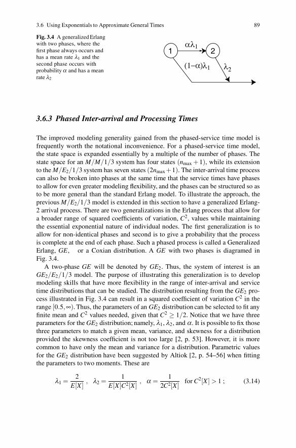
3.6 Using Exponentials to Approximate General Times 89
Fig. 3.4 A generalized Erlangwith two phases, where thefirst phase always occurs andhas a mean rate λ1 and thesecond phase occurs withprobability α and has a meanrate λ2
(1−α) λ2
αλ1
λ1
1 2
3.6.3 Phased Inter-arrival and Processing Times
The improved modeling generality gained from the phased-service time model isfrequently worth the notational inconvenience. For a phased-service time model,the state space is expanded essentially by a multiple of the number of phases. Thestate space for an M/M/1/3 system has four states (nmax +1), while its extensionto the M/E2/1/3 system has seven states (2nmax +1). The inter-arrival time processcan also be broken into phases at the same time that the service times have phasesto allow for even greater modeling flexibility, and the phases can be structured so asto be more general than the standard Erlang model. To illustrate the approach, theprevious M/E2/1/3 model is extended in this section to have a generalized Erlang-2 arrival process. There are two generalizations in the Erlang process that allow fora broader range of squared coefficients of variation, C2, values while maintainingthe essential exponential nature of individual nodes. The first generalization is toallow for non-identical phases and second is to give a probability that the processis complete at the end of each phase. Such a phased process is called a GeneralizedErlang, GE, or a Coxian distribution. A GE with two phases is diagramed inFig. 3.4.
A two-phase GE will be denoted by GE2. Thus, the system of interest is anGE2/E2/1/3 model. The purpose of illustrating this generalization is to developmodeling skills that have more flexibility in the range of inter-arrival and servicetime distributions that can be studied. The distribution resulting from the GE2 pro-cess illustrated in Fig. 3.4 can result in a squared coefficient of variation C2 in therange [0.5,∞). Thus, the parameters of an GE2 distribution can be selected to fit anyfinite mean and C2 values needed, given that C2 ≥ 1/2. Notice that we have threeparameters for the GE2 distribution; namely, λ1, λ2, and α. It is possible to fix thosethree parameters to match a given mean, variance, and skewness for a distributionprovided the skewness coefficient is not too large [2, p. 53]. However, it is morecommon to have only the mean and variance for a distribution. Parametric valuesfor the GE2 distribution have been suggested by Altiok [2, p. 54–56] when fittingthe parameters to two moments. These are
λ1 =2
E[X ], λ2 =
1E[X ]C2[X ]
, α =1
2C2[X ]for C2[X ] > 1 ; (3.14)
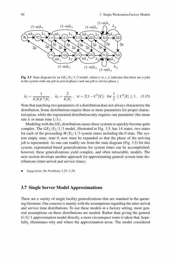
90 3 Single Workstation Factory Models
αλ1 αλ1 αλ1 αλ1
2λ
2λ 2λ 2λ
2μ2μ2μ 2μ 2μ 2μ 2μ
2μ 2μ 2μ 2μ 2μ
(1−α)λ1 (1−α)λ1 (1−α)λ1 (1−α)λ1
2λ 2λαλ1 αλ1 αλ1
(1−α)λ1 (1−α)λ1 2λ (1−α)λ1
Fig. 3.5 State diagram for an GE2/E2/1/3 model, where a (n, i, j) indicates that there are n jobsin the system with one job in arrival phase i and one job is service phase j
λ1 =1
E[X ]C2[X ], λ2 =
2E[X ]
, α = 2(1−C2[X ]) for12≤C2[X ] ≤ 1 . (3.15)
Note that matching two parameters of a distribution does not always characterize thedistribution. Some distributions require three or more parameters for proper charac-terization, while the exponential distribution only requires one parameter (the meanrate λ or mean time 1/λ ).
Modeling with the GE2 distribution causes these systems to quickly become quitecomplex. The GE2/E2/1/3 model, illustrated in Fig. 3.5, has 14 states, two statesfor each of the proceeding M/E2/1/3 system states including the 0 state. The sys-tem empty state, state 0, now must be expanded so that the phase of the arrivingjob is represented. As one can readily see from the state diagram (Fig. 3.5) for thissystem, exponential-based generalizations for system times can be accomplished;however, these generalizations yield complex, and often intractable, models. Thenext section develops another approach for approximating general system time dis-tributions (inter-arrival and service times).
• Suggestion: Do Problems 3.25–3.29.
3.7 Single Server Model Approximations
There are a variety of single facility generalizations that are standard in the queue-ing literature. Our concern is mainly with the assumptions regarding the inter-arrivaland service time distributions. To use these models in a factory setting, more gen-eral assumptions on these distributions are needed. Rather than giving the generalG/G/1 approximation model directly, a more circumspect route is taken that, hope-fully, illuminates why and where the approximation arose. The model considered

3.7 Single Server Model Approximations 91
next is the exact result for the M/G/1 queue, that in a proper form, suggests thestructure of the general approximation result.
3.7.1 General Service Distributions
Consider a single-server system with exponential inter-arrival times, with mean rateλ , and a general service time distribution having mean time 1/μ and variance σ2
s .The state-diagram approach can no longer be used to develop equations that de-fine the steady-state probabilities since these diagrams are tied to the exponentialdistribution or Markovian property. Variations such as Erlang service times can bedeveloped using the state-diagram approach because the Erlang continues with theexponential assumption for the individual phases. The point of view taken for ageneral service process is to observe the system only at service completion times.This allows us to model, using the Markovian properties of the arrival process, thesteady-state system size probabilities at departure points. It turn out that for thisM/G/1 system, the steady-state probabilities at departure points are the same as thesteady-state probabilities at an arbitrary point in time [4, p. 221]. The derivation ofthese probabilities is beyond the scope of this text and involves developing the gen-erating function transform for the departure point probabilities. The development ofthe mean values for the number of jobs in the system was initially obtained inde-pendently in 1932 by Pollaczek and Khintchine and is now considered a standardproperty for general service time queueing systems.
Property 3.1. The Pollaczek and Khintchine, or “P-K”, formula for W IP inan M/G/1 queueing system is given by
W IPs = E[N] =λμ
+
(
λμ
)2+λ 2σ2
s
2(
1− λμ
)
where N is the number of jobs in the system, λ is the mean arrival rate, and theservice distribution has mean and variance given by 1/μ and σ2
s , respectively.
The notation used in the above property is common throughout this text. The sub-script s used with W IP is to emphasize that the mean work-in-process is over theentire system; the subscript s used with the variance is to emphasize that the param-eter refers to the service time distribution and is frequently used to differentiate theservice distribution parameters from the inter-arrival parameters.
One implication of Little’s Law is that for workstations that have one-at-a-timeprocessing, the relationship between the average number in the system and the aver-age number in the queue is given by WIPs−W IPq = λe/μ. Since λe = λ for M/G/1systems, the expected number of jobs waiting for the processing, E[Nq], is
92 3 Single Workstation Factory Models
W IPq = E[Nq] =
(
λμ
)2+λ 2σ2
s
2(
1− λμ
) .
Using Little’s Law one more time, the following important property is obtained, andthis property will be used to develop approximations for more complicated systems.
Property 3.2. The P-K formula for the queue cycle time in an M/G/1 systemis given by
CTq = E[Tq] =WIPq
λ=
(
λμ
)2+λ 2σ2
s
2λ(
1− λμ
)
where Tq is a random variable denoting the time a job spends in the queue, λis the mean arrival rate, and the service distribution has mean and variancegiven by 1/μ and σ2
s , respectively.
The goal is now to rearrange this formula into a form that will be utilized a greatdeal in the development of more realistic factory models. First recall from (1.11)that the squared coefficient of variation is defined by
C2[T ] =V [T ]E[T ]2
so that in terms of service time distribution parameters, we can write
C2s = μ2σ2
s .
Recall from (3.11) and (3.12) that the results for the M/M/1 model are
WIPs(M/M/1) =u
1−u, and
CTs(M/M/1) =1
μ −λ
where u is the server utilization factor and is equal to λ/μ. Here we have introduceda notational convention of writing the model assumptions (i.e., M/M/1) explicitlyin the formula. This convention will be used whenever the context does not makethe model clear. It should not be difficult to show (hint: use (2.1)) the following:
W IPq(M/M/1) =u2
1−u, and
CTq(M/M/1) =u
1−uE[Ts] (3.16)
where Ts is a random variable denoting the time a job spends in the server.
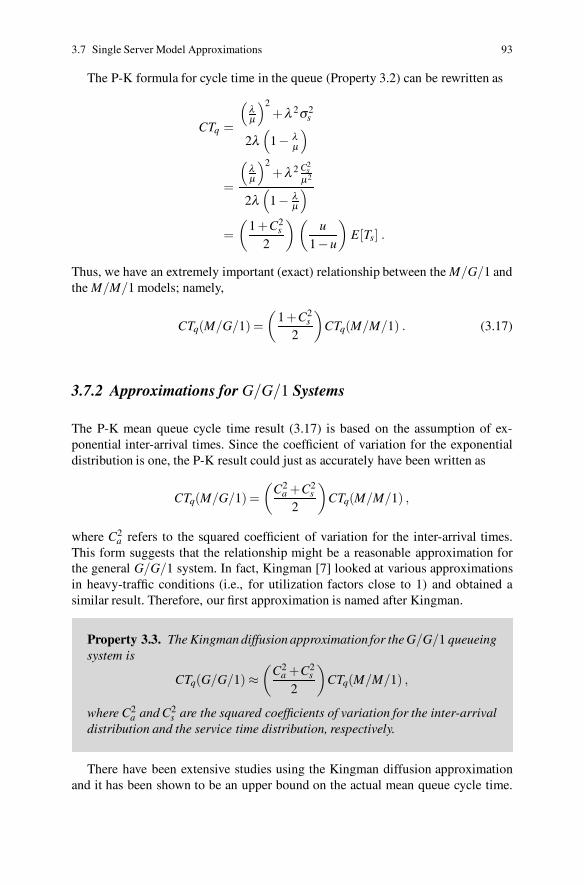
3.7 Single Server Model Approximations 93
The P-K formula for cycle time in the queue (Property 3.2) can be rewritten as
CTq =
(
λμ
)2+λ 2σ2
s
2λ(
1− λμ
)
=
(
λμ
)2+λ 2 C2
sμ2
2λ(
1− λμ
)
=(
1 +C2s
2
) (
u1−u
)
E[Ts] .
Thus, we have an extremely important (exact) relationship between the M/G/1 andthe M/M/1 models; namely,
CTq(M/G/1) =(
1 +C2s
2
)
CTq(M/M/1) . (3.17)
3.7.2 Approximations for G/G/1 Systems
The P-K mean queue cycle time result (3.17) is based on the assumption of ex-ponential inter-arrival times. Since the coefficient of variation for the exponentialdistribution is one, the P-K result could just as accurately have been written as
CTq(M/G/1) =(
C2a +C2
s
2
)
CTq(M/M/1) ,
where C2a refers to the squared coefficient of variation for the inter-arrival times.
This form suggests that the relationship might be a reasonable approximation forthe general G/G/1 system. In fact, Kingman [7] looked at various approximationsin heavy-traffic conditions (i.e., for utilization factors close to 1) and obtained asimilar result. Therefore, our first approximation is named after Kingman.
Property 3.3. The Kingman diffusion approximation for the G/G/1 queueingsystem is
CTq(G/G/1) ≈(
C2a +C2
s
2
)
CTq(M/M/1) ,
where C2a and C2
s are the squared coefficients of variation for the inter-arrivaldistribution and the service time distribution, respectively.
There have been extensive studies using the Kingman diffusion approximationand it has been shown to be an upper bound on the actual mean queue cycle time.
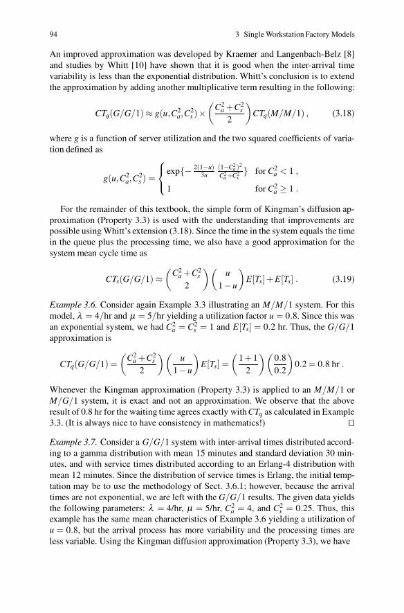
94 3 Single Workstation Factory Models
An improved approximation was developed by Kraemer and Langenbach-Belz [8]and studies by Whitt [10] have shown that it is good when the inter-arrival timevariability is less than the exponential distribution. Whitt’s conclusion is to extendthe approximation by adding another multiplicative term resulting in the following:
CTq(G/G/1)≈ g(u,C2a,C
2s )×
(
C2a +C2
s
2
)
CTq(M/M/1) , (3.18)
where g is a function of server utilization and the two squared coefficients of varia-tion defined as
g(u,C2a,C
2s ) =
⎧
⎨
⎩
exp{− 2(1−u)3u
(1−C2a )2
C2a +C2
s} for C2
a < 1 ,
1 for C2a ≥ 1 .
For the remainder of this textbook, the simple form of Kingman’s diffusion ap-proximation (Property 3.3) is used with the understanding that improvements arepossible using Whitt’s extension (3.18). Since the time in the system equals the timein the queue plus the processing time, we also have a good approximation for thesystem mean cycle time as
CTs(G/G/1) ≈(
C2a +C2
s
2
)(
u1−u
)
E[Ts]+E[Ts] . (3.19)
Example 3.6. Consider again Example 3.3 illustrating an M/M/1 system. For thismodel, λ = 4/hr and μ = 5/hr yielding a utilization factor u = 0.8. Since this wasan exponential system, we had C2
a = C2s = 1 and E[Ts] = 0.2 hr. Thus, the G/G/1
approximation is
CTq(G/G/1) =(
C2a +C2
s
2
)(
u1−u
)
E[Ts] =(
1 +12
)(
0.80.2
)
0.2 = 0.8 hr .
Whenever the Kingman approximation (Property 3.3) is applied to an M/M/1 orM/G/1 system, it is exact and not an approximation. We observe that the aboveresult of 0.8 hr for the waiting time agrees exactly withCTq as calculated in Example3.3. (It is always nice to have consistency in mathematics!) ��
Example 3.7. Consider a G/G/1 system with inter-arrival times distributed accord-ing to a gamma distribution with mean 15 minutes and standard deviation 30 min-utes, and with service times distributed according to an Erlang-4 distribution withmean 12 minutes. Since the distribution of service times is Erlang, the initial temp-tation may be to use the methodology of Sect. 3.6.1; however, because the arrivaltimes are not exponential, we are left with the G/G/1 results. The given data yieldsthe following parameters: λ = 4/hr, μ = 5/hr, C2
a = 4, and C2s = 0.25. Thus, this
example has the same mean characteristics of Example 3.6 yielding a utilization ofu = 0.8, but the arrival process has more variability and the processing times areless variable. Using the Kingman diffusion approximation (Property 3.3), we have
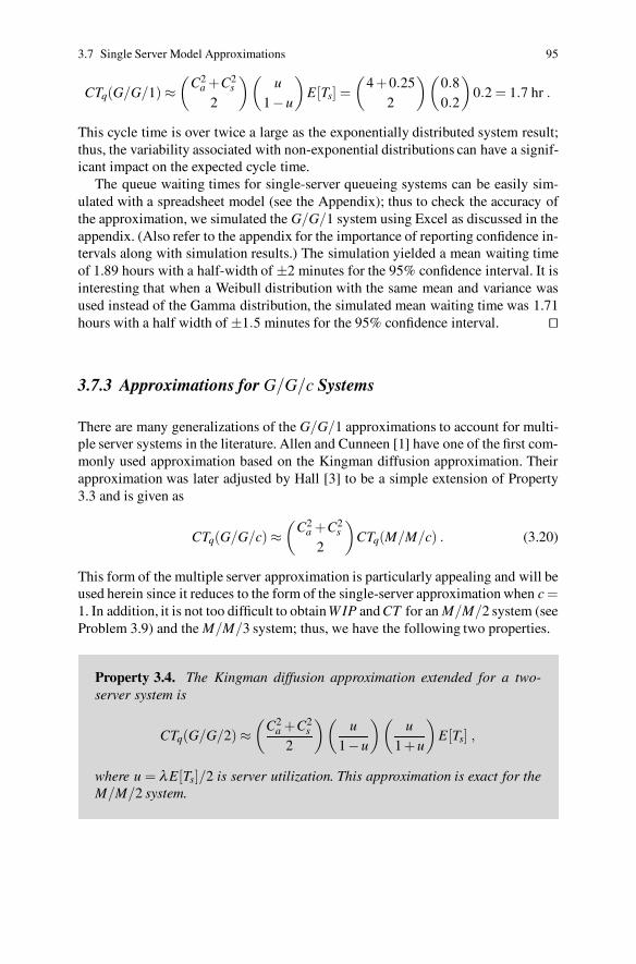
3.7 Single Server Model Approximations 95
CTq(G/G/1) ≈(
C2a +C2
s
2
)(
u1−u
)
E[Ts] =(
4 +0.252
)(
0.80.2
)
0.2 = 1.7 hr .
This cycle time is over twice a large as the exponentially distributed system result;thus, the variability associated with non-exponential distributions can have a signif-icant impact on the expected cycle time.
The queue waiting times for single-server queueing systems can be easily sim-ulated with a spreadsheet model (see the Appendix); thus to check the accuracy ofthe approximation, we simulated the G/G/1 system using Excel as discussed in theappendix. (Also refer to the appendix for the importance of reporting confidence in-tervals along with simulation results.) The simulation yielded a mean waiting timeof 1.89 hours with a half-width of ±2 minutes for the 95% confidence interval. It isinteresting that when a Weibull distribution with the same mean and variance wasused instead of the Gamma distribution, the simulated mean waiting time was 1.71hours with a half width of ±1.5 minutes for the 95% confidence interval. ��
3.7.3 Approximations for G/G/c Systems
There are many generalizations of the G/G/1 approximations to account for multi-ple server systems in the literature. Allen and Cunneen [1] have one of the first com-monly used approximation based on the Kingman diffusion approximation. Theirapproximation was later adjusted by Hall [3] to be a simple extension of Property3.3 and is given as
CTq(G/G/c) ≈(
C2a +C2
s
2
)
CTq(M/M/c) . (3.20)
This form of the multiple server approximation is particularly appealing and will beused herein since it reduces to the form of the single-server approximation when c =1. In addition, it is not too difficult to obtainW IP and CT for an M/M/2 system (seeProblem 3.9) and the M/M/3 system; thus, we have the following two properties.
Property 3.4. The Kingman diffusion approximation extended for a two-server system is
CTq(G/G/2) ≈(
C2a +C2
s
2
)(
u1−u
)(
u1 +u
)
E[Ts] ,
where u = λ E[Ts]/2 is server utilization. This approximation is exact for theM/M/2 system.

96 3 Single Workstation Factory Models
Property 3.5. The Kingman diffusion approximation extended for a three-server system is
CTq(G/G/3) ≈(
C2a +C2
s
2
)(
u1−u
)(
3u2
2 +4u +3u2
)
E[Ts] ,
where u = λ E[Ts]/3 is server utilization. This approximation is exact for theM/M/3 system.
An approximation proposed in Hopp and Spearman [5] uses the following ap-proximation for a Markovian multiple server system from [9]
CTq(M/M/c) =
(
u√
2c+2−2
c
)
CTq(M/M/1) .
The resulting approximation of Hopp and Spearman yields a general extension as:
Property 3.6. The Kingman diffusion approximation extended for a multi-server system is
CTq(G/G/c) ≈(
C2a +C2
s
2
)
(
u√
2c+2−1
c(1−u)
)
E[Ts] ,
where u = λ E[Ts]/c is server utilization.
Finally, we repeat the obvious rule for system cycle time (3.19) extended to amultiple-server system that holds whenever service is one-at-a-time:
CTs(G/G/c) = CTq(G/G/c)+E[Ts] . (3.21)
Example 3.8. Consider again the system of Example 3.7 except for a two-serversystem and with a mean service time of 24 minutes. Thus, server utilization staysthe same (namely, u = 0.8) and the squared coefficients of variation are still given asC2
a = 4 and C2s = 0.25. Then the expected system cycle time using the approximation
of Property 3.6 is
CTq(G/G/2) ≈(
4 +0.252
)
(
(0.8)√
6−1
2(1−0.8)
)
0.4
= 1.54 hr .
If we use Property 3.4, the approximation becomes
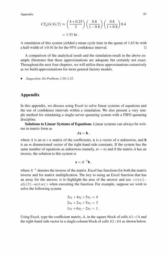
Appendix 97
CTq(G/G/2) ≈(
4 +0.252
)(
0.81−0.8
)(
0.81 +0.8
)
0.4
= 1.51 hr .
A simulation of this system yielded a mean cycle time in the queue of 1.63 hr witha half-width of ±0.01 hr for the 95% confidence interval. ��
A comparison of the analytical result and the simulation result in the above ex-ample illustrates that these approximations are adequate but certainly not exact.Throughout the next four chapters, we will utilize these approximations extensivelyas we build approximations for more general factory models.
• Suggestion: Do Problems 3.30–3.32.
Appendix
In this appendix, we discuss using Excel to solve linear systems of equations andthe use of confidence intervals within a simulation. We also present a very sim-ple method for simulating a single-server queueing system with a FIFO queueingdiscipline.
Solutions to Linear Systems of Equations. Linear systems can always be writ-ten in matrix form as
Ax = b ,
where A is an m×n matrix of the coefficients, x is a vector of n unknowns, and bis an m dimensioned vector of the right-hand-side constants. If the system has thesame number of equations as unknowns (namely, m = n) and if the matrix A has aninverse, the solution to this system is
x = A−1b ,
where A−1 denotes the inverse of the matrix. Excel has functions for both the matrixinverse and for matrix multiplication. The key to using an Excel function that hasan array for the answer, is to highlight the area of the answer and use <ctrl-shift-enter> when executing the function. For example, suppose we wish tosolve the following system:
3x1 +4x2 +5x3 = 4
2x1 +2x2 +5x3 = 3
1x1 +6x2 −2x3 = 1 .
Using Excel, type the coefficient matrix, A, in the square block of cells A2:C4 andthe right-hand-side vector in a single column block of cells E2:E4 as shown below.
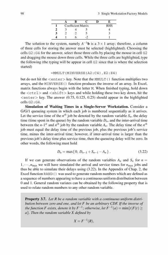
98 3 Single Workstation Factory Models
A B C D E1 Coefficient Matrix RHS2 3 4 5 43 2 2 5 34 1 6 -2 1
The solution to the system, namely A−1b is a 3× 1 array; therefore, a columnof three cells for storing the answer must be selected (highlighted). Choosing thecells G2:G4 for the answer, select those three cells by placing the mouse in cell G2and dragging the mouse down three cells. While the three cells are highlighted, typethe following (the typing will be appear in cell G2 since that is where the selectionstarted)
=MMULT(MINVERSE(A2:C4),E2:E4)
but do not hit the <enter> key. Note that the MMULT() function multiplies twoarrays, and the MINVERSE() function produces the inverse of an array. In Excel,matrix functions always begin with the letter M. When finished typing, hold downthe <ctrl> and <shift> keys and while holding these two key down, hit the<enter> key. The answer (0.75, 0.125, 0.25) should appear in the highlightedcells G2:G4.
Simulation of Waiting Times in a Single-Server Workstation. Consider aG/G/1 queueing system in which each job is numbered sequentially as it arrives.Let the service time of the nth job be denoted by the random variable Sn, the delaytime (time spent in the queue) by the random variable Dn, and the inter-arrival timebetween the n-1st and nth job by the random variable An. The delay time of the nth
job must equal the delay time of the previous job, plus the previous job’s servicetime, minus the inter-arrival time; however, if inter-arrival time is larger than theprevious job’s delay time plus service time, then the queueing delay will be zero. Inother words, the following must hold
Dn = max{0, Dn−1 +Sn−1 −An } . (3.22)
If we can generate observations of the random variables An and Sn for n =1, · · · ,nmax we will have simulated the arrival and service times for nmax jobs andthus be able to simulate their delays using (3.22). In the Appendix of Chap. 2, theExcel functionRAND() was used to generate random numbers which are defined asa sequence of numbers appearing to have a continuous uniform distribution between0 and 1. General random variates can be obtained by the following property that isused to relate random numbers to any other random variable.
Property 3.7. Let R be a random variable with a continuous uniform distri-bution between zero and one, and let F be an arbitrary CDF. If the inverse ofthe function F exists, denote it by F−1; otherwise, let F−1(a) = min{t |F(t)≥a}. Then the random variable X defined by
X = F−1(R),
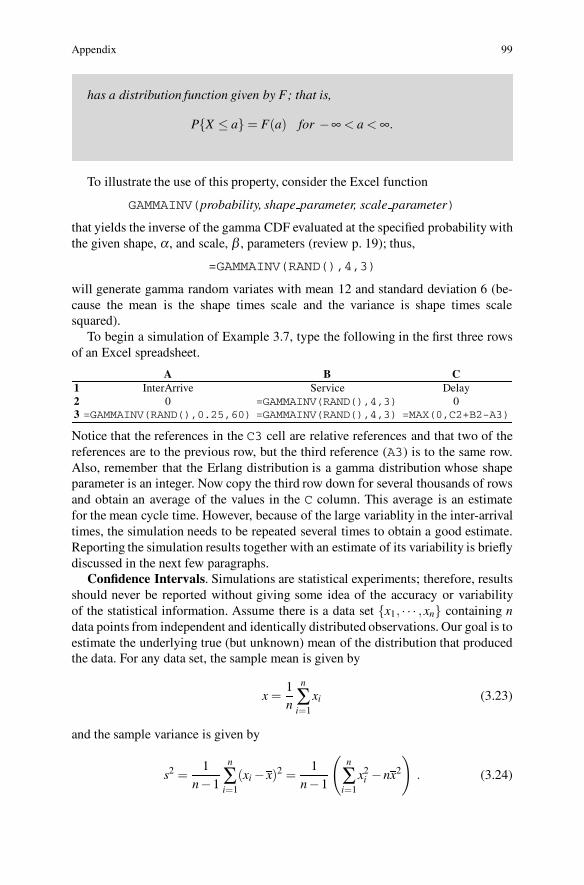
Appendix 99
has a distribution function given by F; that is,
P{X ≤ a} = F(a) for −∞ < a < ∞.
To illustrate the use of this property, consider the Excel function
GAMMAINV(probability, shape parameter, scale parameter)
that yields the inverse of the gamma CDF evaluated at the specified probability withthe given shape, α, and scale, β , parameters (review p. 19); thus,
=GAMMAINV(RAND(),4,3)
will generate gamma random variates with mean 12 and standard deviation 6 (be-cause the mean is the shape times scale and the variance is shape times scalesquared).
To begin a simulation of Example 3.7, type the following in the first three rowsof an Excel spreadsheet.
A B C1 InterArrive Service Delay2 0 =GAMMAINV(RAND(),4,3) 03 =GAMMAINV(RAND(),0.25,60) =GAMMAINV(RAND(),4,3) =MAX(0,C2+B2-A3)
Notice that the references in the C3 cell are relative references and that two of thereferences are to the previous row, but the third reference (A3) is to the same row.Also, remember that the Erlang distribution is a gamma distribution whose shapeparameter is an integer. Now copy the third row down for several thousands of rowsand obtain an average of the values in the C column. This average is an estimatefor the mean cycle time. However, because of the large variablity in the inter-arrivaltimes, the simulation needs to be repeated several times to obtain a good estimate.Reporting the simulation results together with an estimate of its variability is brieflydiscussed in the next few paragraphs.
Confidence Intervals. Simulations are statistical experiments; therefore, resultsshould never be reported without giving some idea of the accuracy or variabilityof the statistical information. Assume there is a data set {x1, · · · ,xn} containing ndata points from independent and identically distributed observations. Our goal is toestimate the underlying true (but unknown) mean of the distribution that producedthe data. For any data set, the sample mean is given by
x =1n
n
∑i=1
xi (3.23)
and the sample variance is given by
s2 =1
n−1
n
∑i=1
(xi − x)2 =1
n−1
(
n
∑i=1
x2i −nx2
)
. (3.24)

100 3 Single Workstation Factory Models
Since an estimate for the true mean is desired, the temptation may be to reportthe sample mean only; however, a single value will provide an estimate but it givesno information on the variability of the estimate. To include information about vari-ability, a confidence interval is often used. For example, a 95% confidence intervalfor the mean implies that if the same experiment were repeated 100 times, approx-imately 95 of those confidence intervals would contain the true mean; that is, weexpect to be correct approximately 19 out of 20 times.
Under the assumption of normally distributed data and unknown variance, the1−α confidence interval for the mean is given by
(xn − tn−1, α2
sn√n
, xn + tn−1, α2
sn√n) (3.25)
where tn−1,α/2 is a critical value based on the Student-t distribution. Statistical testsare usually better as the degrees-of-freedom increases. (As a rule of thumb, a statis-tical test loses a degree-of-freedom whenever a parameter must be estimated by thedata set; thus, the t-test has only n−1 degrees-of-freedom instead of n because weuse the data to estimate the variance.)
If using Excel, the function =TINV(0.05, 24) would yield the critical valuefor a 95% t-statistic for a sample of 25 data points. Notice that Excel automaticallysplits the error into a right-hand error and a left-hand error; thus, if it were desiredto obtain the critical value for a 90% confidence interval of a sample of 100 points,the function =TINV(0.10, 99) would be used. (As an historical note: whenstatistical tables were primarily used to obtain the critical value for the statistics, therule of thumb was to use the z-statistic for large sample sizes; however, with Excel,there is no reason to switch to the z-statistic since Excel does not have a problemwith large sample sizes.)
When applying confidence intervals to simulations, care must be taken not toviolate the independence assumption. Because sequential output from a simulationare usually correlated, it is best to form a random sample by performing severalreplicates of the same simulation, where each replicate starts with a different randomnumber seed. The random sample for the confidence interval then comes from thesummary statistics of each replicate.
Problems
3.1. Consider a facility open 24 hours per day with a single machine that is usedto service only one type of job. The company policy is to limit the number of jobswithin the facility at any one time to 4. The mean arrival rate of jobs is 120 jobs perday, and the mean processing time for a job is 15 minutes. Both the processing andinter-arrival times are assumed to be exponentially distributed. Answer the follow-ing questions regarding the long-run behavior of the facility.(a) What is the average number of jobs that arrive to the facility (but not necessarilyget in) per hour?
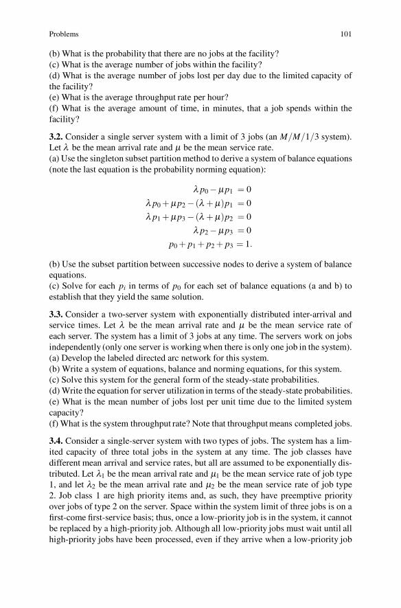
Problems 101
(b) What is the probability that there are no jobs at the facility?(c) What is the average number of jobs within the facility?(d) What is the average number of jobs lost per day due to the limited capacity ofthe facility?(e) What is the average throughput rate per hour?(f) What is the average amount of time, in minutes, that a job spends within thefacility?
3.2. Consider a single server system with a limit of 3 jobs (an M/M/1/3 system).Let λ be the mean arrival rate and μ be the mean service rate.(a) Use the singleton subset partition method to derive a system of balance equations(note the last equation is the probability norming equation):
λ p0 −μ p1 = 0
λ p0 + μ p2 − (λ + μ)p1 = 0
λ p1 + μ p3 − (λ + μ)p2 = 0
λ p2 −μ p3 = 0
p0 + p1 + p2 + p3 = 1.
(b) Use the subset partition between successive nodes to derive a system of balanceequations.(c) Solve for each pi in terms of p0 for each set of balance equations (a and b) toestablish that they yield the same solution.
3.3. Consider a two-server system with exponentially distributed inter-arrival andservice times. Let λ be the mean arrival rate and μ be the mean service rate ofeach server. The system has a limit of 3 jobs at any time. The servers work on jobsindependently (only one server is working when there is only one job in the system).(a) Develop the labeled directed arc network for this system.(b) Write a system of equations, balance and norming equations, for this system.(c) Solve this system for the general form of the steady-state probabilities.(d) Write the equation for server utilization in terms of the steady-state probabilities.(e) What is the mean number of jobs lost per unit time due to the limited systemcapacity?(f) What is the system throughput rate? Note that throughput means completed jobs.
3.4. Consider a single-server system with two types of jobs. The system has a lim-ited capacity of three total jobs in the system at any time. The job classes havedifferent mean arrival and service rates, but all are assumed to be exponentially dis-tributed. Let λ1 be the mean arrival rate and μ1 be the mean service rate of job type1, and let λ2 be the mean arrival rate and μ2 be the mean service rate of job type2. Job class 1 are high priority items and, as such, they have preemptive priorityover jobs of type 2 on the server. Space within the system limit of three jobs is on afirst-come first-service basis; thus, once a low-priority job is in the system, it cannotbe replaced by a high-priority job. Although all low-priority jobs must wait until allhigh-priority jobs have been processed, even if they arrive when a low-priority job
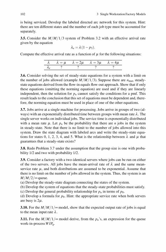
102 3 Single Workstation Factory Models
is being serviced. Develop the labeled directed arc network for this system. Hint:there are ten different states and the number of each job type must be accounted forseparately.
3.5. Consider the M/M/1/3 system of Problem 3.2 with an effective arrival rategiven by the equation
λe = λ (1− p3).
Compute the effective arrival rate as a function of μ for the following situations:
λ λ = μ λ = 2μ λ = 3μ λ = 4μλe ? ? ? ?
3.6. Consider solving the set of steady-state equations for a system with a limit onthe number of jobs allowed (example M/M/1/3). Suppose there are nmax steady-state equations derived from the flow-in equals flow-out approach. Show that if onlythese equations (omitting the norming equation) are used and if they are linearlyindependent, then the solution for pn cannot satisfy the conditions for a pmf. Thisresult leads to the conclusion that this set of equations must be dependent and, there-fore, the norming equation must be used in place of one of the other equations.
3.7. Jobs arrive at a single machine for processing. Jobs arrive in groups of two (al-ways) with an exponentially distributed time between groups with mean rate λ . Thesingle server works on individual jobs. The service time is exponentially distributedwith a mean rate μ. Let pn be the probability that there are n jobs in the systemin steady-state. Note that there is no limit to the number of jobs allowed into thissystem. Draw the state diagram with labeled arcs and write the steady-state equa-tions for states 0, 1, 2, 3, 4, and 5. What is the relationship between λ and μ thatguarantees that a steady-state exists?
3.8. Redo Problem 3.7 under the assumption that the group size is one with proba-bility 1/2 and two with probability 1/2.
3.9. Consider a factory with a two-identical servers where jobs can be run on eitherof the two servers. All jobs have the mean-arrival rate of λ and the same mean-service rate μ, and both distributions are assumed to be exponential. Assume thatthere is no limit on the number of jobs allowed in the system. Thus, the system is anM/M/2/∞ queue.(a) Develop the steady-state diagram connecting the states of the system.(b) Develop the system of equations that the steady-state probabilities must satisfy.(c) Develop the general probability relationship for pn in terms of p0.(d) Develop a formula for p0. Hint: the appropriate service rate when both serversare busy is 2μ.
3.10. For the M/M/1/∞ model, show that the expected output rate of jobs is equalto the mean input rate λ .
3.11. For the M/M/1/∞ model derive, from the pn’s, an expression for the queuework-in-process W IPq.

Problems 103
3.12. Using Little’s Law, obtain the cycle time in the queue, CTq, from the result ofProblem 3.11.
3.13. The cycle time in the system is logically the cycle time in the queue plus theexpected service time
CTs = CTq +E[Ts].
For the M/M/1/∞ model derive an expression for CTq using the CTs result ofEq. (3.12).
3.14. Consider an M/M/1/∞ system with a mean arrival rate of λ = 5 jobs per hour.Compute the system performance measures (W IPs, CTs, ths, u) for several differentservice rates μ ∈ {5.5,6,7,8,9,10}. Graph the WIPs and CTs as a function of thesystem utilization factor u.
3.15. Determine the impact of an arrival rate of 5 per day in Example 3.4 (λ =5, μ = 3, γ = 2 in Eq. 3.13) as it reflects on the system parameters.(a) Write the system of equations for the steady-state probabilities.(b) Obtain the system performance measures: CTs, CTq, W IPs, W IPq, utilization u,mean service time E[Ts], and throughput λe.
3.16. For a system with non-identical service rates (see Sect. 3.5) and a limit of Njobs in the system (Eq. 3.13), obtain an expression for the mean service time per job,E[Ts], as a function of the mean throughput rate λe, the steady-state probabilities pn
and the mean-service rates μ and γ.
3.17. Solve Problem 3.16 for the probabilities given the parameters: nmax = 4, λ = 3,μ = 3, and γ = 2.
3.18. Consider a two-server system with non-identical machines, exponentially dis-tributed inter-arrival and service times, and a limit of four jobs. The mean inter-arrival rate is λ . The mean service rates are γ < μ. Jobs cannot be split across ma-chines. When there is not a queue of waiting jobs and the faster machine completesprocessing first, the job on the slower machine is immediately moved to the fastermachine to complete processing.(a) Develop the steady-state diagram of the number of jobs in the system and theflow rates between states.(b) Develop the system of equations describing the steady-state probabilities of be-ing in each state.(c) Solve this system of equations.
3.19. For Problem 3.18, obtain the system parameters: CTs, CTq, W IPs, WIPq, u,mean service time E[Ts], the expected number of busy servers (EBS), and throughputths.
3.20. A workstation has two different machines for performing two distinct pro-cessing tasks. The workstation has one operator that performs all work done in the
104 3 Single Workstation Factory Models
workstation on all jobs. That is, the operator stays with a job and moves it from ma-chine to machine to accomplish the necessary processing. Jobs arrive to the worksta-tion at a mean rate λ (exponentially distributed inter-arrival times). Each job is firstprocessed by the operator on Machine 1 which takes an exponentially distributedlength of time with mean rate μ. Then the job and operator go to Machine 2 for fur-ther processing. The processing time on the second machine is also exponentiallydistributed but with a mean rate γ. The operator works on one job at a time andcompletes it before starting on a new job. The company limits the jobs in this work-station to 3.(a) Define an appropriate state space representation for this model.(b) Using your state space, develop a state diagram to model this situation.(c) Write the utilization equation for machine one, using the state probabilities.(d) Write the operator utilization equation, using the state probabilities.(e) Write the workstation work-in-process equation, using the state probabilities.(f) Write the throughput equation, using the state probabilities.
3.21. A company has a special purpose processing area that makes parts usedthroughout the company. A variety of different parts are made on a single machineand transported to various locations within the company for storage until they areneeded in that area. The company has a very experienced employee who does theanalysis of the parts currently available throughout the company and then decideswhat part type is to be made next at this machine. The part-needs analysis and re-lease for processing is performed by this employee in two steps. The needs-analysisstep takes 1/2 hour on average, but with the variety of parts to be analyzed, this timeis exponentially distributed. Historical data indicates that 7 of every 9 parts analysesresults in a standard part-type release and, since the part processing information isalready on file, the part order is then released to the machine immediately.
Two of every nine analyses, however, results in the need for a special-purposepart for which the processing data are not available. Thus, this employee then devel-ops a complete processing plan for the part. This processing plan development timeaverages an additional 2.5 hours. Due to the variety of the special purpose parts, ithas been observed that this extra preparation time also is exponentially distributed.The order development employee is additionally charged with keeping the flow ofjobs within the machine area reasonably smooth and timely. Towards this objective,the employee has developed the following release strategy. If there are 3 part ordersalready in the machining area, the employee holds the current completed order at herdesk until a part has been completed and shipped. Then the “ready” order is givento the machine area personnel. If there is a completed (but blocked) order on theanalyses employee’s desk, no new order analysis is started until the blocked orderhas been cleared and been released to the machining area.
The machining area has only one machine and the average time for processingan order is 70 minutes. Due to the variety of part types, this processing time isexponentially distributed.
Develop a model of the special parts processing workstation (order analysesthrough processing). This encompasses the analyses employee and the machine(there is an operator for the machine and it is not necessary to keep track of this

Problems 105
operator). First draw a diagram of every possible configuration that this workstationcan encounter. From this set of configurations, develop a state-space representa-tion for these configurations. Then draw a rate-connected state diagram relating allof these configurations. Develop the steady-state equations for the rate-state dia-gram. Solve these equations for the steady-state probabilities. And finally, developthe workstation performance measures for this problem (machine utilization, order-development employee utilization, and throughput).
3.22. Consider an E2/M/1/3 model with the arrival rate of 3 jobs per hour anda service rate of 4 jobs per hour. Compute the steady state probabilities and thesystem performance measures of utilization, CTs, W IPs, and throughput. Note thatthis system has a capacity of 3 jobs.
3.23. Consider an E2/M/1/4 model with the arrival rate of 3 jobs per hour anda service rate of 4 jobs per hour. Compute the steady state probabilities and thesystem performance measures of utilization, CTs, W IPs, and throughput. Note thatthis system has a capacity of 4 jobs.
3.24. Solve Problem 3.21 using a spreadsheet such as Excel.
3.25. Find the parameters of an GE2 approximation for a random variable X withspecified mean and squared coefficient of variation:
Case E[X ] C2[X ] λ1 α λ2
i 1 5/4ii 4/3 3/2iii 5 2iv 5/8 5/2
3.26. Develop a model of an M/GE2/1/3 system and compute the system perfor-mance measures given the mean arrival rate is 0.2/hr and the service distribution hasparameters E[S] = 5 hr and C2[S] = 2.
3.27. Develop a model of an M/GE2/1/3 system and compute the system perfor-mance measures given the mean arrival rate is 3/hr and the service distribution hasparameters μ = 3/hr, α = 0.5, and γ = 4/hr.
3.28. Solve Problems 3.25 and 3.26 using a spreadsheet such as Excel.
3.29. Develop the node-arc diagram for an M/GE2/2/3 system (identical ma-chines).
3.30. Using the approximation of Eq. 3.19, compute the cycle time in an M/G/1system for three systems with the same arrival rates of λ = 4 and service timesE[Ts] = 0.2, but different squared coefficients of variation (C2[Ts] = 1/2,1,2).
3.31. Using the data from Problem 3.29, except for λ , develop a graph of the systemWIPs over the utilization from 0.1 to 0.95 in steps of 0.05. Insert three curves intothe graph, based on the squared coefficients of variation (C2[Ts] = 0.5,1,2).

106 3 Single Workstation Factory Models
3.32. Using the approximation of Property 3.6 and Eq. (3.21), compute the cycletime in the system for three systems with the same mean arrival rates of λ = 4 andmean service times of E[Ts] = 0.4, but different squared coefficients of variation(C2[Ts] = 1/2,1,2). Note here that one machine is not adequate since u > 1, soassume that there are two-identical machines available, i.e., use an M/G/2 system.
3.33. Consider a single-server system with two types of jobs. The system has a lim-ited capacity of three total jobs in the system at any time. The job classes havedifferent mean arrival and service rates, but all are assumed to be exponentially dis-tributed. Let λ1 be the mean arrival rate and μ1 be the mean service rate of JobType 1, and let λ2 be the mean arrival rate and μ2 be the mean service rate of JobType 2. Jobs are served on a first-come first-serve basis (denoted as FCFS or FIFO).(a) Develop the labeled directed arc network for this system. Hint: there are fifteendifferent states and the sequence of job types in the queue must be maintained.(b) Write the equations linking the steady-state probabilities.(c) Write a formula for computing (in terms of the pi’s) the total WIPs, WIPs byproduct type, throughput, throughput by product type, the system CTs, CTs by prod-uct type.
3.34. Consider a single-server system with two types of jobs. The system has alimited capacity of three total jobs in the system at any time. The job classes havedifferent mean arrival and service rates, but all are assumed to be exponentiallydistributed. Let λ1 be the mean arrival rate and μ1 be the mean service rate of JobType 1, and let λ2 be the mean arrival rate and μ2 be the mean service rate of JobType 2. Jobs are served on a non-preemptive priority basis with job type 1 givenpreference; that is, once a job starts it can not be displaced from the machine.(a) Develop the labeled directed arc network for this system. Hint: there are thirteendifferent states and the sequence of job types in the queue will always be Type 1’sin front of Type 2’s.(b) Write the equations linking the steady-state probabilities.(c) Write a formula for computing (in terms of the pi’s) the total WIPs, WIPs byproduct type, throughput, throughput by product type, the system CTs, and CTs byproduct type.
3.35. Team Computer Project. Consider a situation (factory) where there is a limitof 4 jobs allowed at any time; arrivals to a full system are lost. Assume that all inter-arrival and processing times are exponentially distributed with mean rates specified.Job processing has two steps (Step 1 uses Machine 1 and Step 2 uses Machine 2).That is, there are two independent processing steps that must be done in the se-quence: Machine 1 then Machine 2. The system is automated with-respect-to jobmovement between the queue and machines and between machines and then fromthe last machine to shipping (not part of this problem). There currently is no spacefor a job to wait for processing at Machine 2 after it has completed processing at Ma-chine 1. Therefore, the completed job is left on Machine 1 until Machine 2 becomesavailable.
Management would like to improve the factory throughput and they are wantto know what throughput improvement could be gained if they would invest in a

References 107
Current System
Proposed System
Example
= blocked after service completion
Fig. 3.6 Two configurations for Problem 3.35
conveyor between the machines. Develop a model and obtain the throughput forthis system under the following two parameter sets: λ = 6, μ1 = 8, μ2 = 7 andλ = 9, μ1 = 6, μ2 = 6. Contrast the system throughput with and without a singlebuffer (job holding station) between the two machines for both configurations (seeFig. 3.6).
Develop a computer code to solve these two problems and evaluate the systemthroughput. Make it general in that the rate parameters are input or specified valueswithin the spreadsheet that can be changed (such as merely changing parametervalues between the data sets).
3.36. Model an E2/M/1/3 system with a dependent arrival process in that once thesystem is full, the arrival process is shutoff until space is available in the system.
References
1. Allen, A.O. (1978). Probability, Statistics, and Queueing Theory: With Computer ScienceApplications, Academic Press, New York.
2. Altiok, T. (1996). Performance Analysis of Manufacturing Systems, Springer-Verlag, NewYork.
3. Hall, R.W. (1991). Queueing Methods: For Services and Manufacturing, Prentice-Hall, En-glewood Cliffs, N. J.
4. Gross, D., and Harris, C.M. (1998). Fundamentals of Queueing Theory, Third Edition, JohnWiley & Sons, New York.
5. Hopp, W.J. and Spearman M.L. (1996).Factory Physics: Foundationsof ManufacturingMan-agement, Irwin, Chicago.
6. Kendall, D.G. (1953). Stochastic Processes Occurring in the Theory of Queues and TheirAnalysis by the Method of Imbedded Markov Chains. Annals of Mathematical Statistics,24:338–354.
7. Kingman, J.F.C. (1962). On queues in heavy traffic. J. Royal Statist. Soc. Ser. B, 32:102–110.8. Kraemer, W. and Langenbach-Belz, M. (1976). Approximate Formulae for the Delay in the
Queueing System GI/G/1. Congressbook, Eighth Int. Teletraffic Cong., Melbourne.
108 3 Single Workstation Factory Models
9. Sakasegawa, H. (1977). An Approximation Formula Lq = αβρ (1−ρ). Annuals of the Insti-tute of Statistical Mathematics, 29:67–75.
10. Whitt, W. (1983). The Queueing Network Analyzer. The Bell System Technical Journal,62:2779–2814.
Chapter 4Processing Time Variability
In the previous chapter, an approximation for the cycle time in a system queue wasdeveloped (or waiting time in the queue for a machine). The relationship consistsof four parameters. These are the squared coefficient of variation of the inter-arrivaltime process (C2
a), the squared coefficient of variation of the service time process(C2
s ), the machine utilization (u), and the mean service time (E[Ts]). This relationshipis
CTq(G/G/1) =(C2
a +C2s )
2
(
u1−u
)
E[Ts] . (4.1)
From this relationship, it is clear that reducing one of the variability components,C2
a or C2s , will reduce the cycle time in the queue. What might be overlooked is that
reducing variability is equivalent to reducing the machine utilization by some factorwith respect to the mean cycle time measure. In more direct terms, reducing processvariability is equivalent to finding extra capacity in the system since a reduction ofutilization with a constant arrival rate implies an increase in the mean processingrate.
To illustrate the equivalence between reducing variability and utilization, con-sider a single machine system with the following parameter values:
C2a = 1
C2s = 1
u = 0.8
E[Ts] = 2 hr .
Thus the cycle time in the queue CTq is thus
CTq =(1 +1)
2
(
0.81−0.8
)
2 hr = 8 hr .
Now if C2s is reduced by 10% to 0.9, the resulting cycle time is 7.6 hours, a reduc-
tion of 5%. It would take a reduction in machine utilization from 80% to 79.17%
109
110 4 Processing Time Variability
to accomplish this same cycle time decrease if C2s was not changed. Thus, reducing
service time variability (or inter-arrival time variability) has the same effect as ob-taining additional machine capacity. The equivalent utilization factor u is found bysolving the equation
(1 +1)2
(
u1−u
)
2 = 7.6,
4.6u = 3.6,
u = 0.7917.
Now a 50% reduction in the service time variability for this example data wouldreduce the cycle time measure to 6 hours. The equivalent machine utilization factorfor 6 hours given the original system parameters is 0.75. This is a reduction in uti-lization, or the mean service time, of 6.25%. Either of these changes would result ina cycle time in the queue of 6 hours which is a 25% reduction from the original 8hours.
The conclusion that can be drawn from this analysis is that reducing compo-nent variability is equivalent to increasing system capacity when measured by cycletime response. So it is very important to concentrate on reducing variability for theinter-arrival and service time processes since these reductions are like finding “free”machine capacity.
There are many factors that contribute to the variability of the length of time thata job spends in processing. The term “in processing” indicates that the job has con-trol of the machine and other jobs cannot be processed until this job is completed.Job residence time includes the actual time that the machine is processing the job(herein called the natural processing time to distinguish it from the total time on themachine), any setup needed to place the job on the machine and prepare the machinefor the particular job type, any delay due to the unavailability of an operator once themachine is available for allocation to that specific job, and delays due to machinebreakdowns and repairs. Scheduled maintenance is normally accounted for in theavailable machine time rather than accounting for this lost time as part of a specificjob’s residence time. The principle contributors to job residence time variability are:
• Natural processing time variability — the variability evident in the time it takesto actually process a specific job type.
• Random breakdowns and repairs during processing — the variability of the timebetween breakdowns and the variability of the time to repair a broken machine.
• Operator unavailability can induce random delays in the time a job spends “incontrol of” a machine. This time delay occurs when a machine and job are avail-able with the operator being needed to setup the machine and start processing,but the operator is busy serving another machine/job combination.
• Job class setup and take-down times — the time caused by a job-type change ona machine. This change-over time generally occurs at the end of processing ofone job type and the starting of a different job class.

4.1 Natural Processing Time Variability 111
The variability associated with job class setup times is generally for a group ofjobs and, in Chap. 7, this delay and associated variability component is modeledas an aspect of batch-type processing. Operator availability and their impacts onsystem performance is also a complex interaction between the number of operatorsservicing a set of machines. For the most part, this level of detail will be omittedwhen complex factory models are developed. However, in the last section of thischapter, a model of this type of multiple resource interaction is illustrated. Con-cise approximations for quantifying this factor are not available at this time. Thus,the main objective of this chapter is the analysis of the impacts of “natural” pro-cessing time variability and breakdown/repair induced variability on workstationperformance measures such as cycle time and work-in-process.
4.1 Natural Processing Time Variability
Consider a job with processing time random variable, T , with known mean and vari-ance parameters E[T ] and V [T ], respectively. If the processing time is made up ofseveral separate tasks, then there is a good opportunity to reduce the total process-ing time variability by reducing the variability of the individual tasks. Of course,one can directly attempt to reduce the total processing time variability. This is moreconsistently accomplished when there are sub-tasks that can be studied separatelyor possibly assigned to different workers for manual task operations. To illustratethis point, consider that the natural processing time random variable T is made upof three separate (independent) sub-tasks. Hence,
E[T ] = E[T1]+E[T2]+E[T3]V [T ] = V [T1]+V [T2]+V [T3]
C2[T ] =V [T ]E[T ]2
.
Additionally consider that these three sub-processes times are independent and iden-tically distributed random variables so that
E[T ] = 3E[T1]V [T ] = 3V [T1] .
Hence, the individual processing time random variables Ti, for i = 1,2,3, have dis-tributional parameters
E[Ti] =E[T ]
3
V [Ti] =V [T ]
3.
112 4 Processing Time Variability
Furthermore, the squared coefficient of variation of the individual tasks are
C2[Ti] =V [Ti]E[Ti]2
=V [T ]/3
E[T ]2/32 = 3C2[T ], for i = 1,2,3 .
So if the total processing time is made up of three identical sub-tasks, then thesquared coefficient of variation of the individual tasks is actually three times thatof the total time squared coefficient of variation. Now suppose in the analyses ofthe individual tasks it is found that their variability, as measured by C2[Ti], can bereduced to that of the total processing time variability. Then the overall processingtime squared coefficient of variation C2[T ] would be reduced by 1/3.
Example 4.1. Consider a natural processing time that is exponentially distributedwith a mean time of 3 hours. Thus, the squared coefficient of variation C2[T ] is equalto one. Now further assume that this job consists of three distinct but identicallydistributed sub-tasks. Then these sub-tasks have processing times random variablesTi that have distributional parameters E[Ti] = 1 and V [Ti] = 3, for each i, by theabove analysis.
After further study of the three sub-tasks, it is found that the variability of eachtask can be substantially reduced and the resulting times are i.i.d. exponentiallydistributed times each with a mean of one hour. (It is assumed that these variabilitiescan be reduced while the mean processing times remain unchanged.) Thus, C2[Ti] =1, for each sub-task i. The impact on the variability of the total processing timerandom variable T is significant. The parameters are now
E[Ti] = 1
C2[Ti] = 1
V [Ti] = 1 .
Thus, the total processing time random variable now has parameters
E[T ] =3
∑i=1
E[Ti] = 3
V [T ] =3
∑i=1
V [Ti] = 3
C2[T ] =332 = 1/3 .
For this example, the total processing time variability was reduced to 13 of its
original value. This reduction in processing time variability will in turn reduce theassociated workstation cycle time in the queue by 1
6 (why?). So in essence extraprocessing capability has been found (that is, this new system is equivalent in cycletime response to a system with a faster processing time). ��
• Suggestion: Do Problems 4.1–4.3.
4.2 Random Breakdowns and Repairs During Processing 113
4.2 Random Breakdowns and Repairs During Processing
A major source of processing time variability is due to the breakdown of an operat-ing machine and the subsequent delay while the machine is being repaired. Severalcourses of action might result from the breakdown of a machine. The job undergoingprocessing at the time of the breakdown might not be recoverable (i.e., lost), the jobmight require additional processing before resumption of “normal” processing, orthe job might not be effected by the breakdown and normal processing can resumeimmediately after the repair is complete (as if the breakdown never occurred). Onlythe latter case is considered herein, although for the second case, the additional pro-cessing time needed to resume service can be included in the machine repair timeso that the second and third situations become equivalent.
The assumption being made is that once a machine has been repaired after abreakdown, the job that was processing at the time of the breakdown is continuedas if the breakdown never occurred. Thus, a breakdown merely extends the job pro-cessing time (actually job residence time with the ”normal” processing time beingunaffected). When breakdowns occur, they obviously impact the job residence timeon the machine and the resulting job residence time distribution needs to be devel-oped. This is called the effective processing time to distinguish it from the normalprocessing time.
Definition 4.1. The effective processing time, Te, refers to the time that a job firsthas control of the processor until the time at which the job releases the processor sothat it is available to begin work on another job.
Only the mean and variance parameters of the effective processing time randomvariable are needed and not the distribution itself. For this development, a givenjob has several possibilities. The job can complete processing without a breakdowninterruption, the machine could breakdown once during service, the machine couldbreakdown twice during service, etc. So the effective processing time is also a ran-dom variable given by
Te = T +N
∑i=1
Ri , (4.2)
where T is the normal (uninterrupted) processing time random variable, the Ri’sare the (i.i.d.) repair time random variables, and N is the random number of fail-ures during the service time T . The number of failures N is a function of the timebetween failures random variables, Fi, for the machine in question and is assumedindependent of the actual time that it takes to do the repairs, Ri.
A key parameter needed for expressing the effect of failures and repairs on ser-vice times is the availability of the processor.
Definition 4.2. The availability, a, of a processor that is subject to failures is thelong-run average fraction of time that the processor is available for processing jobs.
114 4 Processing Time Variability
Using the notation above, it is not difficult to express availability in terms of themean time to failure and the mean repair time.
Property 4.1. Processor availability is determined by
a =E[F1]
E[F1]+E[R1]
where F1,F2, · · · and R1,R2, · · · are i.i.d. random variables representing suc-cessive failure times and successive repair times, respectively, for the proces-sor.
Hopp and Spearman [2] developed an expression for the mean and variance of theeffective service time for processors that are less than 100% reliable under the as-sumption that failures are exponentially distributed:
E[Te] =E[Ts]
a, and (4.3)
C2e = C2[Te] = C2
s +(1 +C2[R1])a(1−a)E[R1]
E[Ts]. (4.4)
They show that when Te and C2e are used in place of Ts and C2
s in (4.1) the formulagives an exact expression for the mean waiting time in the queue for a workstationdescribed by an M/G/1 system subject to exponential failures. (Notice that whenTe replaces Ts, the utilization factor must be adjusted as well.) For other G/G/csystems, it serves as an approximation.
Example 4.2. Consider a single workstation with jobs arriving according to a Pois-son process (i.e., exponential inter-arrival times) with an average time between ar-rivals of 75 minutes. Initially we ignore the fact that the machine at the workstationis not 100% reliable and observe that the normal processing time is described by anErlang type-3 distribution with mean of 58 minutes; thus, Ca = 1, E[Ts] = 58 min,Cs = 1/3, and u = 58/75 = 0.7733. These parameters used in (4.1) yield CTq = 132min.
After presenting these results, we are told that the processing machine is not com-pletely reliable. The time between machine breakdowns is exponentially distributedwith a mean time of 3 hours measured according to machine processing time anddoes not include idle time. The repair time is distributed according to a lognormaldistribution with a mean time of 30 min and a standard deviation of 15 min yieldinga squared coefficient of variation of 0.25 for the repair time. The availability is thusgiven by
a =E[F1]
E[F1]+E[R1]
=3
3 +1/2= 0.85714 .
115
The mean of the effective processing time (4.3) is
E[Te] =E[T ]
a= 67.67 min ,
and the squared coefficient of variation for the effective processing time (4.4) is
C2[Te] =13
+(1 +0.25)(0.85714)(1−0.85714)(30)
58= 0.4125 .
The effective mean service time yields an effective utilization of u = 67.67/75 =0.9023 so that the application of (4.1) results in a revised value for the expectedwaiting time in the queue
CTq =(1 +0.4125)
2
(
0.90231−0.9023
)
67.67 min = 441 min .
Notice that the inclusion of machine failure in the model results in over a three-fold increase in the mean waiting time; thus, to ignore failures can create significanterrors in performance measures. This increase is due to two factors: (1) machinefailures cause an increase the effective utilization factor and (2) machine failurescause an increase in the service variability. As the utilization factor approaches one,small changes in the factor will have major changes in waiting times, and in thiscase, the majority of the increase in waiting times is due to the utilization factorincrease; only about 5%–6% of the increase is due to the increase in service vari-ability. ��
• Suggestion: Do Problems 4.4–4.9 and 4.13–4.14.
Operators are frequently required to setup a machine for each job. Machine prepa-ration time usually takes significantly more time than the job unloading operation.If the machining operation requires a dedicated operator, then most likely the modelof that situation would require only one resource (either the machine or the oper-ator). When an operator is used only part time during processing and the operatoris then free to perform other tasks, operators and machines can no longer be mod-eled as one. In this situation, an operator is frequently assigned control of more thanone machine and, thus, is responsible for setting up jobs on several machines. If anoperator is assigned to cover too many machines then system performance can besignificantly degraded because of delays resulting from waiting for the operator tobecome available to perform the necessary job setups. Even when the operator isassigned to cover only two machines, some delays will be encountered due to the
4.2 Random Breakdowns and Repairs During Processing
116 4 Processing Time Variability
timing of job completions. If a system has reasonable capacity, then the operator ma-chine interaction problem does not significantly impact system performance. Thus,this level of detail is frequently omitted in system models. This interaction can, how-ever, degrade system performance significantly if overlooked. The operator-machineinteraction problem also offers an opportunity to illustrate how multiple resource in-teractions can be quantified and evaluated.
In the modeling assumptions, only one job class is treated with two identicalmachines and one operator. In addition, to simplify the analysis as much as possible,exponentially distributed times are assumed for job inter-arrival times, job setuptimes, and job processing times. Since we need to keep track of two resources,namely the operator and the machines, a state space that only keeps a record of thenumber of jobs in the system does not carry enough information to appropriatelyestablish the true system state. Specifically, in addition to the number of jobs in thesystem, the status of each machine-job combination must be known; that is, the stateof the system must include whether the job is “in setup” or “in processing”. If twojobs are in the “in setup” status, then only one of them can be actually proceedingwith setup because there there is only one operator.
There is often more than one way to define a state space, so that the particulardefinition chosen is up to the modeler. It is good practice to choose a state spacedefinition that is descriptive so that the individual defining equations for the steady-state probabilities will be easy to read. One descriptive state definition is to use athree-tuple for the states. Each state is represented as (n, i, j), where n denotes thenumber of jobs in the system and i and j indicate the status of the two machines.There are three possible values for i and j: 0 indicates a machine has no job as-sociated with it, s indicates that a machine has a job “in setup”, and p indicates amachine has a job “in process”. For example, the state (1, s,0) indicates that thereis one job in the system and the operator is setting it up on a machine, state (5, s, s)indicates that there are 5 jobs in the system with one job being set-up on a machine,another job waiting at a machine for the operator, and 3 jobs waiting in the queue fora machine, and state (7, p, p) indicates 7 jobs in the system with both machines busyprocessing, 5 jobs queued, and the operator idle. Because the machines are identi-cal, it is not necessary to know which machine is processing and which machine isbegin setup.
The state space representation for n ≥ 2 is made up of three individual states:(n, s, s), (n, s, p), and (n, p, p). For n = 0, there is no need for all three indices, butfor consistency this state is denoted as (0,0,0). For n = 1, the possible states are(1, s,0) and (1, p,0). The states of the system, grouped by number of jobs in thesystem, are
{(0,0,0),(1,s,0),(1, p,0),(2,s,s), (2,s, p),(2, p, p),(3,s,s), (3,s, p),(3, p, p), · · ·} .
The inter-arrival time, setup time, and service time distributions are all assumedto be exponentially distributed. The mean rates for these three processes are denotedby λ , γ, and μ, respectively. Note that if both machines are processing (indepen-dently), the mean output rate for the system is 2μ. If both machines are being setup,
117
the mean setup rate is γ, not 2γ, because there is only one operator. The equationsrelating the steady-state probabilities for this system are:
λ p(0,0,0) = μ p(1,p,0)
(λ + γ)p(1,s,0) = λ p(0,0,0) + μ p(2,s,p)
(λ + μ)p(1,p,0) = γ p(1,s,0) +2μ p(2,p,p)
(λ +2μ)p(2,p,p) = γ p(2,s,p)
(λ + γ)p(2,s,s) = λ p(1,s,0) + μ p(3,s,p)
(λ + γ + μ)p(2,s,p) = λ p(1,p,0) + γ p(2,s,s) +2μ p(3,p,p)
(λ +2μ)p(3,p,p) = λ p(2,p,p) + γ p(3,s,p)
(λ + γ)p(3,s,s) = λ p(2,s,s) + μ p(4,s,p) (4.5)
(λ + γ + μ)p(3,s,p) = λ p(2,s,p) + γ p(3,s,s) +2μ p(4,p,p) (4.6)
(λ +2μ)p(4,p,p) = λ p(3,p,p) + γ p(4,s,p) (4.7)
...
(λ + γ)p(n,s,s) = λ p(n−1,s,s) + μ p(n+1,s,p)
(λ + γ + μ)p(n,s,p) = λ p(n−1,s,p) + γ p(n,s,s) +2μ p(n+1,p,p)
(λ +2μ)p(n+1,p,p) = λ p(n,p,p) + γ p(n+1,s,p)
...
plus the norming equation, which is the sum of all probabilities equal to one. Theset of three numbered equations (4.5–4.7) are repeated with increasing indices. Thelast three listed equations represent these equations for the index n (where n ≥ 3).So the system has an infinite number of defining equations with the first seven beingspecial and all others being one of three possible general forms.
The numerical solution scheme employed is rather straightforward, but unfortu-nately, the solution cannot be represented nicely in closed form. For specified valuesof the parameter set (λ , γ, μ), the system is solved in the following fashion. The un-known p(0,0,0) is set 1.0, then all other probabilities can be solved recursively fornumerical values according to the procedure described in the next paragraph. Sincewe have an infinite system, it will be truncated to a finite set of probabilities at thepoint that the probabilities become very small. Thus, we continue to find proba-bilities until the individual probability terms become very small. At that point, westop and determine the sum of all probabilities that have been calculated. The finalanswer then becomes the individual terms divided by this sum.
The process for evaluating the individual probabilities is actually rather straight-forward. First given p(0,0,0) the first equation is used to obtain p(1,p,0). Then, us-ing three equations at a time, the probabilities groups solved in turn are: thegroup (p(1,s,0), p(2,s,p), p(2,p,p)), then the group (p(2,s,s), p(3,s,p), p(3,p,p)) and finally(p(3,s,s), p(4,s,p), p(4,p,p)). Each of these sets is found from the solution of three linearequations. This last set of three equations is repeated solved for (p(n−1,s,s), p(n,s,p),
4.2 Random Breakdowns and Repairs During Processing

118 4 Processing Time Variability
p(n,p,p)) for increasing values of n until the sum of the three values are less thatsome limit. The solution of each of these three distinct sets of equations needs onlyvalues for previously obtained probabilities. Thus, starting with one assumed value,p(0,0,0), as many probabilities as necessary can be obtained; after the relative valuesfor these probabilities have been determined, they are normed to sum to one. Onefurther observation is that only one 3× 3 matrix inverse is needed since the samematrix reoccurs as the coefficients of the unknowns for all three forms of the threeequations groups.
To be more specific, we first observe that p(1,p,0) = (λ/μ)p(1,0,0). The the secondthrough fourth equations can be rewritten in matrix form as
⎡
⎣
−(λ + γ) μ 0γ 0 2μ0 γ −(λ +2μ)
⎤
⎦
⎡
⎣
p(1,s,0)p(2,s,p)p(2,p,p)
⎤
⎦=
⎡
⎣
−λ p(0,0,0)(λ + μ)p(1,p,0)
0
⎤
⎦ ,
with its solution given by
⎡
⎣
p(1,s,0)p(2,s,p)p(2,p,p)
⎤
⎦=
⎡
⎣
−(λ + γ) μ 0γ 0 2μ0 γ −(λ +2μ)
⎤
⎦
−1⎡
⎣
−λ p(0,0,0)(λ + μ)p(1,p,0)
0
⎤
⎦ . (4.8)
Once the values of the probabilities (p(1,s,0), p(2,s,p), p(2,p,p)) have been obtained, thevector (p(2,s,s), p(3,s,p), p(3,p,p)) is solved similarly using the fifth through seventhequations in the system. This solution is written as
⎡
⎣
p(2,s,s)p(3,s,p)p(3,p,p)
⎤
⎦=
⎡
⎣
−(λ + γ) μ 0γ 0 2μ0 γ −(λ +2μ)
⎤
⎦
−1⎡
⎣
−λ p(1,s,0)λ p(1,p,0)− (λ + μ + γ)p(2,s,p)
λ p(2,p,p)
⎤
⎦ .
(4.9)Equations (4.5–4.7) can now be used to yield the general form of the solution forn ≥ 3; namely,
⎡
⎣
p(n,s,s)p(n+1,s,p)p(n+1,p,p)
⎤
⎦=
⎡
⎣
−(λ + γ) μ 0γ 0 2μ0 γ −(λ +2μ)
⎤
⎦
−1⎡
⎣
−λ p(n−1,s,s)λ p(n−1,s,p)− (λ + μ + γ)p(n,s,p)
λ p(n,p,p)
⎤
⎦ .
(4.10)Notice that the solution to each system always involves the same inverse whichgreatly simplifies the computational burden of the process.
Not all values for the three parameters will yield a system that can be solved. Ifthe operator sets up too slowly or if the arrival rates are too fast for the processingtimes, the queues will build up continually and no steady-state is possible. Althoughdeveloping the steady-state conditions is outside the scope of this text, they aregiven in [1] and, for completeness, we state them below. Steady-state probabilitieswill exist if and only if the three parameter values are such that
119
2(μ + γ)μγ2μ2 +2μγ + γ2 < λ .
Example 4.3. To illustrate the methodology and computations, consider a two-machine system with one server. Let the mean arrival rate of jobs be 1 per hour,the mean time to perform a setup by 15 minutes, and let the mean processing timebe 90 minutes. Recall that all the times are exponentially distributed. Thus, λ = 1,γ = 4, and μ = 2/3. The matrix that needs to inverted, and its inverse, are
⎡
⎣
−(λ + γ) μ 0γ 0 2μ0 γ −(λ +2μ)
⎤
⎦
−1
=
⎡
⎣
−0.1622 0.0473 0.02700.2838 0.3547 0.20270.4865 0.6081 −0.0811
⎤
⎦ .
Now setting p(0,0,0) to 1.0 yields p(1,p,0) = 1.5. Using (4.8), the first set of threeprobabilities are
(p(1,s,0),p(2,s,p), p(2,p,p)) = (0.2804,0.6030,1.0338) .
From these values, (4.9) is used to evaluate the next three probabilities
(p(2,s,s), p(3,s,p),p(3,p,p)) = (0.1082,0.3910,1.1133) .
The probabilities (p(3,s,s), p(4,s,p),p(4,p,p)) are obtained based on these previous val-ues using (4.10) to yield
(p(3,s,s), p(4,s,p),p(4,p,p)) = (0.0637,0.3156,1.0182) .
Repeating the use of (4.10), we obtain
(p(4,s,s), p(5,s,p),p(5,p,p)) = (0.0489,0.2713,0.9014) ,
(p(5,s,s), p(6,s,p),p(6,p,p)) = (0.0413,0.2367,0.7921) ,
...
(p(14,s,s), p(15,s,p),p(15,p,p)) = (0.0110,0.0635,0.2129) .
Stopping at this point, these probabilities sum to 15.288. Dividing all of theseprobabilities by 15.288 yields an approximate solution to this system. It is obviousthat since the probability p(15,p,p) is not very close to zero, that this truncated so-lution will not be very close to the unlimited system solution. In fact using theseprobability values, the estimate for the mean number of jobs, Ns, in the system is
WIP = E[Ns] = 5.606 .
As the number of probabilities obtained is increased, the expected system W IP,converges. These iteration results are displayed below where n denotes the numberof probabilities obtained. Note that it is not much work to increase the number ofprobabilities obtained since they are found iteratively three at a time using (4.10)
4.2 Random Breakdowns and Repairs During Processing
120 4 Processing Time Variability
repeatedly:
n = 20, W IP = 6.399,
n = 30, W IP = 7.263,
n = 40, W IP = 7.603,
n = 50, W IP = 7.725,
n = 60, W IP = 7.658,
n = 70, W IP = 7.779,
n = 80, W IP = 7.783,
n = 90, W IP = 7.785,
n = 100, W IP = 7.785.
The truncated system solution changes very little as more probabilities are addedbeyond the first 80 probabilities. Thus, a reasonable solution to the unlimited systemhas been obtained. The expected cycle time in the system from Little’s Law is
CT = W IP/λ = 7.785 hr .
The expected number of jobs in the operator system is
1×(
p(1,s,0) +∞
∑n=2
p(n,s,p)
)
+2×∞
∑n=2
p(n,s,s) = 0.2819 ,
with the probability that the operator is idle being
p(0,0,0) + p(1,p,0) +∞
∑n=2
p(n,p,p) = 0.75 ,
and the machine utilization factor being
12×(
p(1,p,0) +∞
∑n=2
p(n,s,p)
)
+1×∞
∑n=2
p(n,p,p) = 0.8909 .
The approach of using a truncated system to approximate the unlimited capacitysystem leads to the problem of finding the norming constant by iteratively increas-ing the number allowed in the system until the total non-normed probability sumstabilizes. Using the rate-generator form of the problem for Markov processes, onecan develop a closed form representation of this sum and find the non-normed prob-abilities total sum with the truncation mechanism (see [1]). This approach, however,requires mechanics that will not be developed in this text. ��
• Suggestion: Do Problems 4.10–4.12.
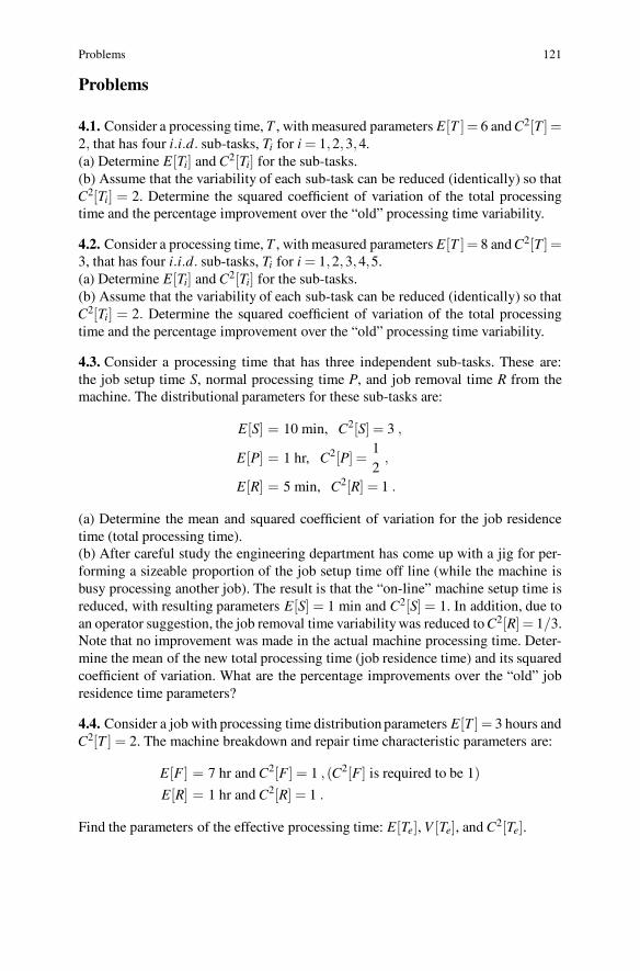
Problems 121
Problems
4.1. Consider a processing time, T , with measured parameters E[T ]= 6 and C2[T ] =2, that has four i.i.d. sub-tasks, Ti for i = 1,2,3,4.(a) Determine E[Ti] and C2[Ti] for the sub-tasks.(b) Assume that the variability of each sub-task can be reduced (identically) so thatC2[Ti] = 2. Determine the squared coefficient of variation of the total processingtime and the percentage improvement over the “old” processing time variability.
4.2. Consider a processing time, T , with measured parameters E[T ]= 8 and C2[T ] =3, that has four i.i.d. sub-tasks, Ti for i = 1,2,3,4,5.(a) Determine E[Ti] and C2[Ti] for the sub-tasks.(b) Assume that the variability of each sub-task can be reduced (identically) so thatC2[Ti] = 2. Determine the squared coefficient of variation of the total processingtime and the percentage improvement over the “old” processing time variability.
4.3. Consider a processing time that has three independent sub-tasks. These are:the job setup time S, normal processing time P, and job removal time R from themachine. The distributional parameters for these sub-tasks are:
E[S] = 10 min, C2[S] = 3 ,
E[P] = 1 hr, C2[P] =12
,
E[R] = 5 min, C2[R] = 1 .
(a) Determine the mean and squared coefficient of variation for the job residencetime (total processing time).(b) After careful study the engineering department has come up with a jig for per-forming a sizeable proportion of the job setup time off line (while the machine isbusy processing another job). The result is that the “on-line” machine setup time isreduced, with resulting parameters E[S] = 1 min and C2[S] = 1. In addition, due toan operator suggestion, the job removal time variability was reduced to C2[R] = 1/3.Note that no improvement was made in the actual machine processing time. Deter-mine the mean of the new total processing time (job residence time) and its squaredcoefficient of variation. What are the percentage improvements over the “old” jobresidence time parameters?
4.4. Consider a job with processing time distribution parameters E[T ] = 3 hours andC2[T ] = 2. The machine breakdown and repair time characteristic parameters are:
E[F ] = 7 hr and C2[F] = 1 , (C2[F] is required to be 1)E[R] = 1 hr and C2[R] = 1 .
Find the parameters of the effective processing time: E[Te], V [Te], and C2[Te].
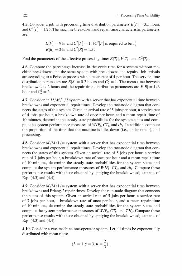
122 4 Processing Time Variability
4.5. Consider a job with processing time distribution parameters E[T ] = 3.5 hoursand C2[T ] = 1.25. The machine breakdown and repair time characteristic parametersare:
E[F ] = 9 hr and C2[F] = 1 , (C2[F] is required to be 1)E[R] = 2 hr and C2[R] = 1.5 .
Find the parameters of the effective processing time: E[Te], V [Te], and C2[Te].
4.6. Compute the percentage increase in the cycle time for a system without ma-chine breakdowns and the same system with breakdowns and repairs. Job arrivalsare according to a Poisson process with a mean rate of 4 per hour. The service timedistribution parameters are E[S] = 0.2 hours and C2
s = 1. The mean time betweenbreakdowns is 2 hours and the repair time distribution parameters are E[R] = 1/3hour and C2
R = 2.
4.7. Consider an M/M/1/3 system with a server that has exponential time betweenbreakdowns and exponential repair times. Develop the rate-node diagram that con-nects the states of this system. Given an arrival rate of 5 jobs per hour, a service rateof 4 jobs per hour, a breakdown rate of once per hour, and a mean repair time of10 minutes, determine the steady-state probabilities for the system states and com-pute the system performance measures of W IPs, CTs, and ths. In addition, computethe proportion of the time that the machine is idle, down (i.e., under repair), andprocessing.
4.8. Consider M/M/1/∞ system with a server that has exponential time betweenbreakdowns and exponential repair times. Develop the rate-node diagram that con-nects the states of this system. Given an arrival rate of 5 jobs per hour, a servicerate of 7 jobs per hour, a breakdown rate of once per hour and a mean repair timeof 10 minutes, determine the steady-state probabilities for the system states andcompute the system performance measures of WIPs, CTs, and ths. Compare theseperformance results with those obtained by applying the breakdown adjustments ofEqs. (4.3) and (4.4).
4.9. Consider M/M/1/∞ system with a server that has exponential time betweenbreakdowns and Erlang-2 repair times. Develop the rate-node diagram that connectsthe states of this system. Given an arrival rate of 5 jobs per hour, a service rateof 7 jobs per hour, a breakdown rate of once per hour, and a mean repair timeof 10 minutes, determine the steady-state probabilities for the system states andcompute the system performance measures of W IPs, CTs, and THs. Compare theseperformance results with those obtained by applying the breakdown adjustments ofEqs. (4.3) and (4.4).
4.10. Consider a two-machine one-operator system. Let all times be exponentiallydistributed with mean rates:
(λ = 1, γ = 3, μ =23) .

References 123
Set p(0,0,0) = 0.0842, and determine the next ten probabilities; that is, p(1,p,0) andthen one set of three probabilities for each of the three equation-set forms similar toEqs. (4.8)–(4.10).
4.11. Develop the system equations for the steady-state probabilities for a singleoperator servicing three machines. What type of difficulties will have to be over-come to solve this system of equations for n → ∞, where n denotes the number ofmachines for which the operator is responsible.
4.12. Consider an infinite capacity 3-machine 2-operator service system where anoperator is required to setup a job on a machine before processing can begin. De-velop the node-arc diagram for 5 or less jobs in the system. That is, develop thediagram explicitly for 0 to 5 jobs in the system with the understanding that the com-plete diagram would contain an infinite number of nodes. All processes, (arrivals,setups and processing) are assumed to be exponentially distributed with mean ratesλ , γ, and μ, respectively.
4.13. Consider an M/M/2/2 system with exponential breakdowns (rate β ) and re-pairs (rate γ). The machines are identical and when one machine breaks down withthe other machine empty, the job being processed is left on the broken machinewhile it is being repaired.
4.14. Consider an M/M/2/2 system with exponential breakdowns (rate β ) and re-pairs (rate γ). The machines are identical and when one machine breaks down withthe other machine empty, the job being processed is moved from the broken machineto the operating machine instantaneously.
References
1. Feldman, R.M., Deuermeyer, B.L., and Valdez-Flores, C. (1993). Utilization of the Method ofLinear Matrix Equations to Solve a Quasi-Birth-DeathProblem, J. Applied Probability,30:639–649.
2. Hopp, W.J., and Spearman M.L. (2000). Factory Physics: Foundations of Manufacturing Man-agement, second edn. IRWIN, Chicago
Chapter 5Multiple-Stage Single-Product Factory Models
The mechanics for developing both exact and approximate single workstation mod-els were developed in Chap. 3. Linking several workstations together is a necessarystep towards more realistic factory models. In this chapter, the single workstationmodels are linked together to form more realistic factory models. The approachtaken is to use general G/G/1 and G/G/c system approximations of Properties3.3 and 3.5 as the building blocks for multiple workstation systems. To properlyconnect a series of workstations, the departure process of jobs from each worksta-tion must be characterized. Specifically, the mean of inter-departure times and theirsquared coefficient of variation must be computed for a workstation. These param-eters then describe the arrival process for the downstream workstation. For generalsystem configurations, there are two basic mechanisms that must be explored: (1)the merging of several input streams into a workstation, and (2) the separation or par-titioning of a workstation output stream into several different streams for differenttarget workstations. This chapter starts with workstations in series and progressesto more complex general network configurations. Single product models are studiedin detail in this chapter and in Chap. 6 the methodology is generalized for multipleproduct systems.
5.1 Approximating the Departure Process from a Workstation
In the study of single workstation models in Chap. 3, the workstation’s impact on theoutput flow of jobs from the workstation was not considered. This information wasnot needed to study the performance of a single workstation, but when the outputfrom one workstation becomes the input to the next workstation, this information iscritical to system analysis. One of the main concerns of this chapter is the impactthat the workstation service and queueing processes have on traffic flow characteris-tics. That is, we will study how the workstation transforms the inter-arrival processcharacteristics into output-stream characteristics. Consider first the mean flow ratefor a system in steady state. In the long run, the same number of units must depart
125

126 5 Multiple-Stage Single-Product Factory Models
the workstation as enter the workstation. Otherwise, there would be a buildup (ordepletion) of jobs in the workstation and the queue would grow infinitely (or unitswould need to be created out of nothing) as time extends to infinity. It may be thatunits are destroyed, but we would account for those units as departing “scrapped”units. Or, it may be that an assembly operation occurs so that the number of unitsappears to change; however, we would consider the assembled unit as two units sothat the net flow of material in is always equal to the net flow out. Applying thisconservation of flow concept, the mean output rate from a workstation must equalthe mean input rate to that workstation.1 The inter-arrival and inter-departure timesrandom variables are denoted as Ta and Td , where the subscripts a and d representarrivals and departures, respectively, for the workstation. Thus, the conservation offlow concept leads to the following property.
Property 5.1. The mean arrival rate of jobs to a workstation operating understeady-state conditions equals the mean departure rate of jobs; that is
E[Ta] = E[Td ] .
For exponential systems, namely M/M/c systems with c ≥ 1, the output processis probabilistically identical to the input process; namely, the inter-departure timesare exponentially distributed so that C2
d = C2a = C2
s = 1. For non-exponential sys-tems, obtaining the value of C2
d is a little more involved. Assume for the momentthat the workstation is extremely busy, then the distribution of the time betweendepartures would essentially be the service time distribution and so C2
d would beexpected to be very close in value to C2
s . At the other extreme, when the systemis very lightly loaded, the inter-departure times should be an arrival time minus theservice time for the last job plus the service time for the arriving job. Thus, the inter-departure time distribution should be similar to the inter-arrival time distribution sothat C2
d should be very similar to C2a . In fact, for an M/G/1 system (remember that
C2a = 1 for M/G/1 systems), Buzacott and Shanthikumar [3] show this is exactly
the correct; namely,C2
d(M/G/1) = 1−u2 +u2C2s , (5.1)
where u is utilization. They also develop for the G/G/1 system a lower bound onC2
d asC2
d(G/G/1) ≥ (1−u)(
1 +uC2a
)
C2a +u2C2
s .
A general relationship for a G/G/1 system for the squared coefficient of variationwas developed by Marshall [4] as
C2d = C2
a +2u2C2s −2u (1−u)CTq/E[Ts] , (5.2)
1 The conservation of flow concept applied to networks is the same as the rate balance conceptused to derive the steady-state probabilities as discussed in Sections 3.1 and 3.2.
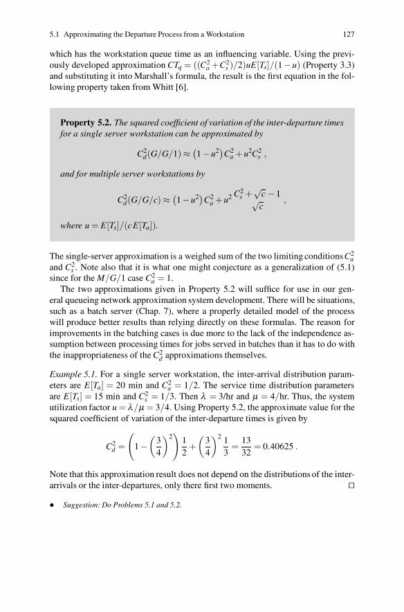
5.1 Approximating the Departure Process from a Workstation 127
which has the workstation queue time as an influencing variable. Using the previ-ously developed approximation CTq = ((C2
a +C2s )/2)uE[Ts]/(1−u) (Property 3.3)
and substituting it into Marshall’s formula, the result is the first equation in the fol-lowing property taken from Whitt [6].
Property 5.2. The squared coefficient of variation of the inter-departure timesfor a single server workstation can be approximated by
C2d(G/G/1) ≈
(
1−u2)C2a +u2C2
s ,
and for multiple server workstations by
C2d(G/G/c) ≈
(
1−u2)C2a +u2 C2
s +√
c −1√c
,
where u = E[Ts]/(cE[Ta]).
The single-server approximation is a weighed sum of the two limiting conditionsC2a
and C2s . Note also that it is what one might conjecture as a generalization of (5.1)
since for the M/G/1 case C2a = 1.
The two approximations given in Property 5.2 will suffice for use in our gen-eral queueing network approximation system development. There will be situations,such as a batch server (Chap. 7), where a properly detailed model of the processwill produce better results than relying directly on these formulas. The reason forimprovements in the batching cases is due more to the lack of the independence as-sumption between processing times for jobs served in batches than it has to do withthe inappropriateness of the C2
d approximations themselves.
Example 5.1. For a single server workstation, the inter-arrival distribution param-eters are E[Ta] = 20 min and C2
a = 1/2. The service time distribution parametersare E[Ts] = 15 min and C2
s = 1/3. Then λ = 3/hr and μ = 4/hr. Thus, the systemutilization factor u = λ/μ = 3/4. Using Property 5.2, the approximate value for thesquared coefficient of variation of the inter-departure times is given by
C2d =
(
1−(
34
)2)
12
+(
34
)2 13
=1332
= 0.40625 .
Note that this approximation result does not depend on the distributions of the inter-arrivals or the inter-departures, only there first two moments. ��
• Suggestion: Do Problems 5.1 and 5.2.
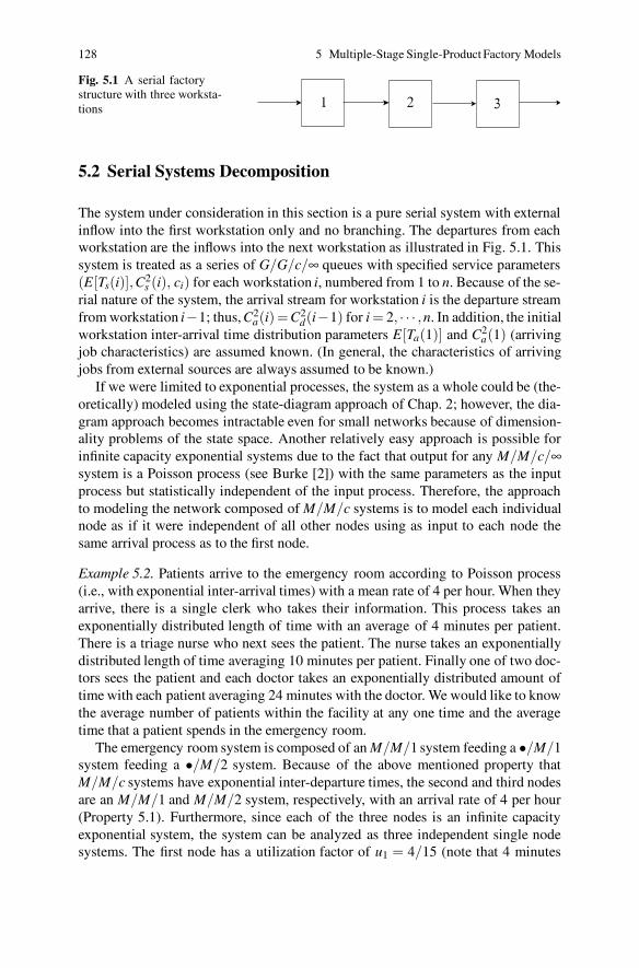
128 5 Multiple-Stage Single-Product Factory Models
Fig. 5.1 A serial factorystructure with three worksta-tions
5.2 Serial Systems Decomposition
The system under consideration in this section is a pure serial system with externalinflow into the first workstation only and no branching. The departures from eachworkstation are the inflows into the next workstation as illustrated in Fig. 5.1. Thissystem is treated as a series of G/G/c/∞ queues with specified service parameters(E[Ts(i)],C2
s (i), ci) for each workstation i, numbered from 1 to n. Because of the se-rial nature of the system, the arrival stream for workstation i is the departure streamfrom workstation i−1; thus, C2
a(i)=C2d(i−1) for i = 2, · · · ,n. In addition, the initial
workstation inter-arrival time distribution parameters E[Ta(1)] and C2a(1) (arriving
job characteristics) are assumed known. (In general, the characteristics of arrivingjobs from external sources are always assumed to be known.)
If we were limited to exponential processes, the system as a whole could be (the-oretically) modeled using the state-diagram approach of Chap. 2; however, the dia-gram approach becomes intractable even for small networks because of dimension-ality problems of the state space. Another relatively easy approach is possible forinfinite capacity exponential systems due to the fact that output for any M/M/c/∞system is a Poisson process (see Burke [2]) with the same parameters as the inputprocess but statistically independent of the input process. Therefore, the approachto modeling the network composed of M/M/c systems is to model each individualnode as if it were independent of all other nodes using as input to each node thesame arrival process as to the first node.
Example 5.2. Patients arrive to the emergency room according to Poisson process(i.e., with exponential inter-arrival times) with a mean rate of 4 per hour. When theyarrive, there is a single clerk who takes their information. This process takes anexponentially distributed length of time with an average of 4 minutes per patient.There is a triage nurse who next sees the patient. The nurse takes an exponentiallydistributed length of time averaging 10 minutes per patient. Finally one of two doc-tors sees the patient and each doctor takes an exponentially distributed amount oftime with each patient averaging 24 minutes with the doctor. We would like to knowthe average number of patients within the facility at any one time and the averagetime that a patient spends in the emergency room.
The emergency room system is composed of an M/M/1 system feeding a •/M/1system feeding a •/M/2 system. Because of the above mentioned property thatM/M/c systems have exponential inter-departure times, the second and third nodesare an M/M/1 and M/M/2 system, respectively, with an arrival rate of 4 per hour(Property 5.1). Furthermore, since each of the three nodes is an infinite capacityexponential system, the system can be analyzed as three independent single nodesystems. The first node has a utilization factor of u1 = 4/15 (note that 4 minutes
5.2 Serial Systems Decomposition 129
per patient is 15 patients per hour) and thus the average number of patients inthe first node is W IP(1) = 4/11 (use Eq. 3.11). The second node has a utiliza-tion factor of u2 = 2/3 yielding WIP(2) = 2 (again use Eq. 3.11). For the thirdnode, we first find the time spent waiting for the doctor. This is given by Prop-erty 3.4 and yields CTq(3) = 42.67 min since u3 = 0.8. Adding the doctor’s timeto the wait time (Eq. 3.21) yields the time spent in third node as CT (3) = 1.11hr. Applying Little’s Law (Property 2.1) gives the average number of patients atthe node as WIP(3) = 4.44. Thus, the total number in the emergency room isWIPs = 4/11+2+4.44 = 6.8. Applying Little’s Law one more time, yields the av-erage value for the total time a patient spends in the emergency room as CTs = 1.7hr. ��
Although the analysis approach used in Example 5.2 is exact only under the as-sumptions of infinite capacity nodes and exponential distributions for inter-arrivalsand processing times, it provides the motivation for approximation schemes whenthese assumptions do not hold. The analysis approach for general systems is basedon the concept that a system’s performance can be adequately approximated by sep-arating the system into individual workstations. The performance characteristics ofthe individual workstations are computed separately and then these results recom-bined for the total system behavior. This decomposition approach is fundamental tothe approximation of general network configurations. The reasons that this decom-position approach is only an approximation are two-fold: first, Property 5.2 is anapproximation and second, the successive inter-departure times are not independentexcept for the M/M/c/∞ case.
The decomposition approach is predicated on being able to establish the indi-vidual workstation parameters needed for using Property 3.3 or 3.6. The requireddata are the parameter set (E[Ts(i)], C2
s (i), ci, E[Ta(i)], C2a(i)) for each workstation
i. The first three parameters are specified data for the workstation. The last two pa-rameters in the set are for the job arrival stream into the workstation. These twointer-arrival distribution parameters need to be estimated from the departure flowsfrom the upstream workstations and, of course, the network structure. For serialsystems, the outflow from one workstation is the direct inflow into the next, so thisparticular serial network topology allows for a sequential computation of these un-known parameters. Starting with the known inflow data into the first workstation,all the necessary data are available and the first workstation’s performance charac-teristics (from Properties 3.3 or 3.6) and the departure stream characteristics (fromProperties 5.2) can be computed. The second workstation arrival stream character-istics are made equal to the first workstation’s departure stream. Thus for the secondworkstation, the performance information and the departure stream parameters areobtained. This becomes the needed information for the third workstation, and soon. (It is now, hopefully, apparent how the topology of the network impacts theanalysis. For a general system structure, the topology is more complex and thesedata must be computed simultaneously leading to the development of a system ofequations as seen in Section 5.4 that must be solved to obtain the inter-arrival distri-bution parameters.) As always, the arrival stream and service characteristics definethe workstation utilization as ui = E[Ts(i)]/(ciE[Ta(i)]).

130 5 Multiple-Stage Single-Product Factory Models
The departure stream characteristics for each workstation consists of the meaninter-arrival time and the squared coefficient of variation of these times. For a se-rial system in steady state, the workstation mean inflow rates must be identical forall workstations. (The assumptions of no losses, no reworks, and one external in-flow point are critical to this simplified method for computing these inflow rates.)Thus, E[Ta(i)] = E[Ta(1)] for all workstations i = 2, · · · ,n. There remains only thetask of computing the C2
d(i) term for each workstation i and the serial structure ofthe network allows for these computations to be carried out sequentially. A recur-sive algorithm can be easily developed for the factory based on the following twoproperties.
Property 5.3. The mean cycle time and departure process for an infinite ca-pacity single-server workstation within a factory that has a pure serial systemtopology are given by
CT (i) ≈(
C2d(i−1)+C2
s (i)2
)(
ui
1−ui
)
E[Ts(i)]+E[Ts(i)] and
C2d(i) ≈
(
1−u2i
)
C2d(i−1)+u2
i C2s (i) ,
where i is the sequence number of the workstation and C2d(0) is the squared
coefficient of variation of the arrival stream to the first workstation. (The onlyarrivals are to the first workstation.)
Property 5.4. The mean cycle time and departure process for an infinite ca-pacity workstation with c servers within a factory that has a pure serial systemtopology are given by
CT (i) ≈(
C2d(i−1)+C2
s (i)2
)
(
u√
2ci+2−1i
ci(1−ui)
)
E[Ts(i)]+E[Ts(i)] and
C2d(i) ≈ 1 +
(
1−u2i
)(
C2d(i−1)−1
)
+u2i
(
C2s (i)−1
)
√ci
,
where i is the sequence number of the workstation and C2d(0) is the squared
coefficient of variation of the arrival stream to the first workstation. (The onlyarrivals are to the first workstation.)
Once the cycle times for the individual workstations have been obtained, theoverall system performance measures can be determined. The cycle time in the to-tal system can be computed for serial systems by merely summing the individualworkstation times since every job visits each workstation exactly once during itsprocessing. This is not a general computation scheme and is, therefore, forgone in

5.2 Serial Systems Decomposition 131
favor of a method that is valid for all network topologies. The more general approachis to use Little’s Law to compute the mean number of jobs, W IPs(i), in each work-station, sum the workstation means together to obtain the total factory mean numberof jobs, W IPs, and then obtain the system mean cycle time through the applicationof Little’s Law again; thus
W IPs =n
∑i=1
W IPs(i) =n
∑i=1
CT (i)E[Ta(i)]
and (5.3)
CTs = E[Ta(1)]×WIPs . (5.4)
Equation (5.3) is independent of the job flow sequence and, hence, valid for anynetwork topology. Notice that for the mean throughput rate, the reciprocal of themean inter-arrival times is used since all arrivals will eventually pass through theworkstation. Equation (5.4) is not very general because it assumes that all arrivalsto the factory enter through the first workstation. In later sections, this may not betrue.
Example 5.3. Consider a three-workstation factory with serial flow as depicted inFig. 5.1. Each workstation has a single machine with the service time distributionparameters as listed in Table 5.1. The inter-arrival time distribution for jobs to the
Table 5.1 Service time characteristics for Example 5.3
Workstation i E [Ts(i)] C2s (i)
1 12 min 2.02 9 min 0.73 13.2 min 1.0
factory has a mean of 15 minutes or a mean rate of 4 jobs per hour, and a squaredcoefficient of variation of 0.75. The system mean work-in-process, cycle time, andthroughput are desired.
Since arrivals to the system occur at the first workstation, E[Ta(1)] = 15 minyielding a utilization factor of u1 = E[Ts(1)]/E[Ta(1)] = 0.8. Using the networkdecomposition principle together with Property 5.3 yields the following for the firstworkstation:
CT (1) =(
C2a(1)+C2
s (1)2
)(
u1
1−u1
)
E[Ts(1)]+E[Ts(1)]
=(
0.75 +2.02
)
0.80.2
(12 min)+12 min
= 78 min = 1.3 hr
C2d(1) =
(
1−u21
)
C2a(1)+u2
1C2s (1)
=(
1−0.82)0.75 +0.82(2.0) = 1.55 , and
132 5 Multiple-Stage Single-Product Factory Models
W IP(1) = CT (1)× 1E[Ta(1)]
=1.3 hr
0.25 hr= 5.2 .
The last equation comes from the application of Little’s Law, and since no jobs arelost, the throughput rate is th = 1/E[Ta(1)]. Notice that care must always be takento make sure that the time units are consistent when applying Little’s Law. Becausethis is a pure serial network, the arrival rate and throughput rate will be the same foreach workstation; thus, the utilization factors for the other two workstations are u2 =E[Ts(2)]/E[Ta(1)] = 0.6 and u3 = E[Ts(3)]/E[Ta(1)] = 0.88. Applying Property 5.3and Little’s Law to the second and third workstations yield
CT (2) =(
1.55 +0.72
)
0.60.4
(0.15 hr)+0.15 hr = 0.403 hr
C2d(2) =
(
1−0.62)1.55 +0.62(0.7) = 1.244
W IP(2) = CT (2)/E[Ta(1)] = 1.613 and
CT (3) =(
1.244 +1.02
)
0.880.12
(0.22 hr)+0.22 hr = 2.030 hr
C2d(3) =
(
1−0.882)1.244 +0.882(1.0) = 1.055
W IPs(3) = CT (3)/E[Ta(1)] = 8.121 .
Finally, the total factory performance characteristics for this serial system are
WIPs = 5.200 +1.613+8.121 = 14.933 jobs
ths =1
E[Ta(1)]= 4/hr
CTs =WIPs
ths= 3.733 hr .
As a comparison, a simulation model was developed for this serial factory struc-ture using Excel. (The appendix of this chapter presents the use of Excel for sim-ulating networks for single-server workstations.) The gamma distribution was usedfor the random inter-arrival times and service times with the appropriate means andsquared coefficients of variations. Five replicates of the model were obtained witheach replication being a simulation of 32,000 customers through the system. Table5.2 displays the analytical approximation results with those obtained from the simu-lation. The analytical approximations are given first followed across the row by thesimulation estimates with the half-width of the 95% confidence interval also shownfor the simulation. (The estimate for the squared coefficients of variation were ob-tained by estimating the variance and dividing by the square of the mean estimate;thus, it is a biased statistic. The confidence interval is based on Eq. (3.25) so it istechnically not correct for ratios; however, it does give some idea of the variabilityof the estimator.)
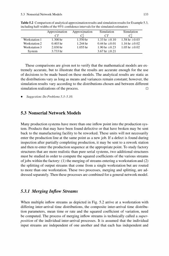
5.3 Nonserial Network Models 133
Table 5.2 Comparison of analytical approximation results and simulation results for Example 5.3,including half-widths of the 95% confidence intervals for the simulated estimators
Approximation Approximation Simulation SimulationCT C2
d CT C2d
Workstation 1 1.300 hr 1.550 hr 1.33 hr ±0.10 1.58 hr ±0.03Workstation 2 0.403 hr 1.244 hr 0.44 hr ±0.01 1.16 hr ±0.02Workstation 3 2.030 hr 1.055 hr 1.90 hr ±0.23 1.05 hr ±0.02
System 3.733 hr 3.67 hr ±0.21
These comparisons are given not to verify that the mathematical models are ex-tremely accurate, but to illustrate that the results are accurate enough for the useof decisions to be made based on these models. The analytical results are static asthe distributions vary as long as means and variances remain constant; however, thesimulation results vary according to the distributions chosen and between differentsimulation realizations of the process. ��
• Suggestion: Do Problems 5.3–5.10.
5.3 Nonserial Network Models
Many production systems have more than one inflow point into the production sys-tem. Products that may have been found defective or that have broken may be sentback to the manufacturing facility to be reworked. These units will not necessarilyenter the production line at the same point as a new job. If a defect is found duringinspection after partially completing production, it may be sent to a rework stationand then re-enter the production sequence at the appropriate point. To study factorystructures that are more realistic than pure serial systems, two additional structuresmust be studied in order to compute the squared coefficients of the various streamsof jobs within the factory: (1) the merging of streams entering a workstation and (2)the splitting of output streams that come from a single workstation but are routedto more than one workstation. These two processes, merging and splitting, are ad-dressed separately. Then these processes are combined for a general network model.
5.3.1 Merging Inflow Streams
When multiple inflow streams as depicted in Fig. 5.2 arrive at a workstation withdiffering inter-arrival time distributions, the composite inter-arrival time distribu-tion parameters, mean time or rate and the squared coefficient of variation, needbe computed. The process of merging inflow streams is technically called a super-position of the individual inter-arrival processes. It is assumed that the individualinput streams are independent of one another and that each has independent and
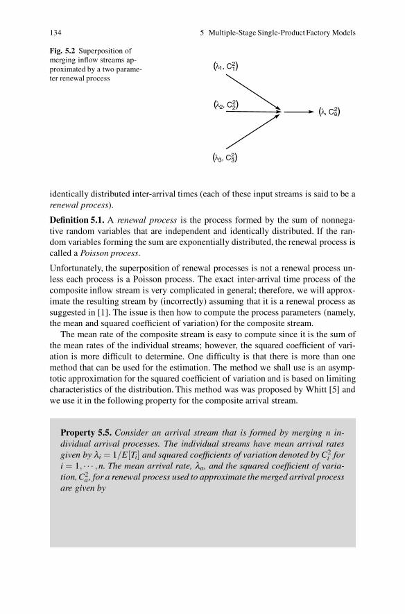
134 5 Multiple-Stage Single-Product Factory Models
Fig. 5.2 Superposition ofmerging inflow streams ap-proximated by a two parame-ter renewal process
( 2, C2) λ 2
( 1, C1) λ 2
( 3, C3) λ 2
( , Ca) λ 2
identically distributed inter-arrival times (each of these input streams is said to be arenewal process).
Definition 5.1. A renewal process is the process formed by the sum of nonnega-tive random variables that are independent and identically distributed. If the ran-dom variables forming the sum are exponentially distributed, the renewal process iscalled a Poisson process.
Unfortunately, the superposition of renewal processes is not a renewal process un-less each process is a Poisson process. The exact inter-arrival time process of thecomposite inflow stream is very complicated in general; therefore, we will approx-imate the resulting stream by (incorrectly) assuming that it is a renewal process assuggested in [1]. The issue is then how to compute the process parameters (namely,the mean and squared coefficient of variation) for the composite stream.
The mean rate of the composite stream is easy to compute since it is the sum ofthe mean rates of the individual streams; however, the squared coefficient of vari-ation is more difficult to determine. One difficulty is that there is more than onemethod that can be used for the estimation. The method we shall use is an asymp-totic approximation for the squared coefficient of variation and is based on limitingcharacteristics of the distribution. This method was was proposed by Whitt [5] andwe use it in the following property for the composite arrival stream.
Property 5.5. Consider an arrival stream that is formed by merging n in-dividual arrival processes. The individual streams have mean arrival ratesgiven by λi = 1/E[Ti] and squared coefficients of variation denoted by C2
i fori = 1, · · · ,n. The mean arrival rate, λa, and the squared coefficient of varia-tion,C2
a, for a renewal process used to approximate the merged arrival processare given by

5.3 Nonserial Network Models 135
λa =n
∑i=1
λi =n
∑i=1
1E[Ti]
C2a =
n
∑i=1
λi
λaC2
i .
Example 5.4. An automated lubricating facility is located in the center of a man-ufacturing plant. Arrivals of parts needing lubrication come from three sources:manufactured parts needing assembly, defective parts that have been disassembledand will be returned for reassembly, and parts coming from a sister manufactur-ing facility in another part of the town. The three arrival streams have been ana-lyzed separately. The mean arrival rates for the three streams are given by the vec-tor (λ1,λ2,λ3) = (13.2/hr,3.6/hr,6.0/hr). The squared coefficients of variation forthe three inflow streams are (C2
1 ,C22,C
23) = (5.0,3.0,2.2). The total inflow into the
workstation is the sum of the individual inflows so that λa = 22.8/hr. The relativeweights, 13.2/22.8, 3.6/22.8, and 6.0/22.8, are thus used to determine the compositeinflow stream’s squared coefficient of variation as
C2a =
13.222.8
5.0 +3.6
22.83.0 +
6.022.8
2.2 = 3.947 .
To compute the mean and standard deviation of the inter-arrival times, rememberthat mean rates and mean times are reciprocals; therefore,
E[Ta] =1
22.8hr = 2.63 min , and
V [Ta] = 3.947(2.632) = 27.30 min2 .
��
• Suggestion: Do Problems 5.11 and 5.12.
5.3.2 Random Splitting of the Departure Stream
Jobs that exit from a workstation can be transferred to different workstations basedon several possibilities. Multiple products can be made by specializing a partiallyprocessed product. Thus, the processing sequences can be identical through somestep at which point the items are branched to their unique completion workstationsor sequence of workstations. Another instance occurs due to quality control testingwith good items continuing on their normal route and bad items being reworkedor corrected at a different workstation before continuing normal processing. If thebranching decision is based on an independent random draw for each job, called a
136 5 Multiple-Stage Single-Product Factory Models
Bernoulli decomposition or a Markovian routing, then the squared coefficients ofvariation for the individual resultant streams is exact and relatively easy to computeas long as the initial stream was a renewal process. Specifically, when a renewalprocess undergoes a Bernoulli decomposition, each individual stream is again a re-newal process. Whitt [6] reminds us that this process ultimately is an approximationbecause in a network of workstations the output process from a workstation “is typ-ically not a renewal process and the splitting is often not according to Markovianrouting.”
To illustrate the computations necessary for obtaining the mean rate and coef-ficient of variation for a stream that is split from another stream, assume that p isthe probability that output from one workstation is directed as an arrival processto a second workstation. The arrival stream to the second workstation is made upof the sum of one or more inter-departure times from the first workstation. That is,if there are N departures from the first workstation between arrivals to the secondworkstation, then the second workstation sees an inter-arrival time that is the sumof those N inter-departure times from the first workstation. The number of depar-tures, N , between routings to the target workstation is obviously a random variable,and is distributed according to a geometric distribution. Thus, the probability massfunction of N is given by
Pr{N = n} = f (n) = p (1− p)n−1 ,n = 1,2, · · · ,
where p is the probability that a given job is routed to the second workstation, inde-pendent of previous or future routings. The characteristics for this geometric randomvariable N (review p. 15) are therefore given by
E[N] =1p
V [N] =1− p
p2 .
To compute the time between visits to the second workstation for jobs departingfrom the first workstation, we define the random variable T as the random sum of Nof the independent and identically distributed inter-departure times, Ti; namely,
T = T1 + · · ·+TN =N
∑i=1
Ti .
Since this is a random sum of i.i.d. random variables, we can use Property 1.9 toobtain the mean and variance of T as
E[T ] =E[T1]
p
V [T ] =V [T1]
p+
(1− p)E[T1]2
p2 .

5.3 Nonserial Network Models 137
Noting that C2[t] = V [T ]/(E[T ])2, it is not too hard to derive the following propertyfor split streams.
Property 5.6. Consider a departure stream from a specified workstation witha mean inter-departure time and coefficient of variation given by E[Td ] andC2
d, respectively. When a job departs from the specified workstation, there is aprobability, p, that the job will be routed to a target workstation. If there are noother arriving streams to the target workstation, then the mean inter-arrivaltime and squared coefficient of variation for arrivals to target workstation aregiven by
E[Ta] =E[Td ]
p
C2a = pC2
d +1− p .
If λd is the mean departure rate of jobs from the specified workstation, themean arrival rate to the target workstation is λa = p λd.
Example 5.5. The fifth workstation within a manufacturing facility performs a qual-ity control check on partially manufactured items. Parts receive an unqualified passfrom the inspector with probability 0.8 and they are then sent to Workstation 6 tocontinue the manufacturing process. Approximately 18% of the time, a part hasa partial pass of the quality check and is sent to Workstation 10 for rework. Andapproximately 2% of the time, a part completely fails the test and is sent to thehazardous waste station for disposal which is designated as Workstation 99. Thethroughput rate for Workstation 5 is 7 jobs per hour and the coefficient of variationfor the inter-departure times is 3. As a notational convention, we let λa(i, j) de-note the mean arrival rate of jobs coming from Workstation i going to Workstationj. Likewise, C2
a(i, j) denotes the squared coefficient of variation for the stream ofjobs from Workstation i feeding into Workstation j. Thus, Property 5.6 yields thefollowing:
λa(5,6) = 0.8×7 = 5.6/hr
C2a(5,6) = 0.8×3 +0.2 = 2.6
λa(5,10) = 0.18×7 = 1.26/hr
C2a(5,10) = 0.18×3 +0.82 = 1.36
λa(5,99) = 0.02×7 = 0.14/hr
C2a(5,99) = 0.02×3 +0.98 = 1.04 .
138 5 Multiple-Stage Single-Product Factory Models
Notice that as a check, the arrival rates can be summed and they must equal thedeparture rate from the original stream before it was split. (As a reminder, such aproperty does not hold for the squared coefficients of variation.) ��
• Suggestion: Do Problem 5.11.
5.4 The General Network Approximation Model
Our goal is to develop a methodology for approximating the system performancemeasures for general factory models. In the serial models studied in the previouschapter, the flow structure was straight forward with no losses between workstationsand no job feedback, no branching or other nonserial complications. To address ageneral factory network connection topology, the possibilities of external flows intoany one of the workstations must be considered along with job feedback branch-ing for rework purposes, splitting of the output from a workstation to different nextworkstations, etc. So workstation inflows can come from a variety of sources, exter-nal as well as other workstations within the factory, and this complication is handledby our flow merging mechanism. Probabilistic branching of workstation outflow re-quires departure stream splitting mechanics. Thus, at this point the fundamentalmechanisms needed to address these more complicated system structures have beendeveloped. The major complication that arrises is the order that the workstationsare sequenced for application of the general decomposition approach. That is, sincethere is no longer sequential flows, parameter dependencies are also not sequen-tial so that equations relating the parameters will have to be solved simultaneouslyinstead of sequentially.
The concept of the decomposition approach to factory analysis is the establish-ment of the individual workstation parameters and then the development of eachworkstation’s behavioral characteristics as a stand-alone analysis. These individ-ual analyses are then merged together to estimate the total system behavior. Thisapproach was readily implemented for a pure serial system since the parameters,such as the inflow stream characteristics, could be sequentially computed. Startingwith a known inflow into the first workstation and based on its service character-istics (mean, squared coefficient of variation, and number of servers), the outflowor departure stream characteristics were computed. Then due to the serial factoryflow structure, these become the characteristics of the inflow stream for the nextworkstation in series. This sequential process of evaluation is repeated until the lastworkstation in the series had been evaluated. Then, of course, the results for theindividual workstations are combined for the system performance estimation. De-termining the mean rates and then squared coefficients of variation for inter-arrivaltimes involve distinct analyses so these are discussed separately in the followingtwo subsections.
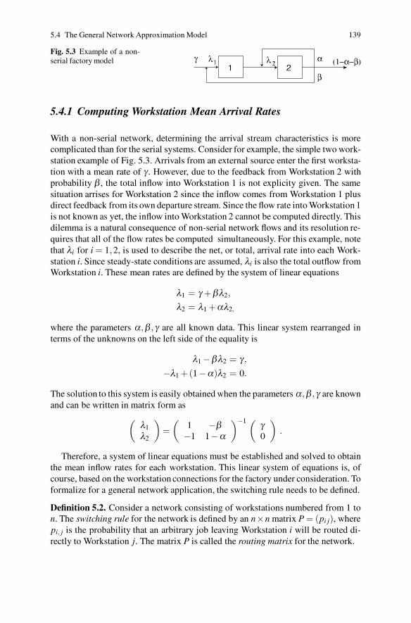
5.4 The General Network Approximation Model 139
Fig. 5.3 Example of a non-serial factory model
5.4.1 Computing Workstation Mean Arrival Rates
With a non-serial network, determining the arrival stream characteristics is morecomplicated than for the serial systems. Consider for example, the simple two work-station example of Fig. 5.3. Arrivals from an external source enter the first worksta-tion with a mean rate of γ. However, due to the feedback from Workstation 2 withprobability β , the total inflow into Workstation 1 is not explicity given. The samesituation arrises for Workstation 2 since the inflow comes from Workstation 1 plusdirect feedback from its own departure stream. Since the flow rate into Workstation 1is not known as yet, the inflow into Workstation 2 cannot be computed directly. Thisdilemma is a natural consequence of non-serial network flows and its resolution re-quires that all of the flow rates be computed simultaneously. For this example, notethat λi for i = 1,2, is used to describe the net, or total, arrival rate into each Work-station i. Since steady-state conditions are assumed, λi is also the total outflow fromWorkstation i. These mean rates are defined by the system of linear equations
λ1 = γ +β λ2,
λ2 = λ1 +αλ2,
where the parameters α,β , γ are all known data. This linear system rearranged interms of the unknowns on the left side of the equality is
λ1 −β λ2 = γ,
−λ1 +(1−α)λ2 = 0.
The solution to this system is easily obtained when the parameters α,β , γ are knownand can be written in matrix form as
(
λ1
λ2
)
=(
1 −β−1 1−α
)−1 ( γ0
)
.
Therefore, a system of linear equations must be established and solved to obtainthe mean inflow rates for each workstation. This linear system of equations is, ofcourse, based on the workstation connections for the factory under consideration. Toformalize for a general network application, the switching rule needs to be defined.
Definition 5.2. Consider a network consisting of workstations numbered from 1 ton. The switching rule for the network is defined by an n×n matrix P = (pi j), wherepi, j is the probability that an arbitrary job leaving Workstation i will be routed di-rectly to Workstation j. The matrix P is called the routing matrix for the network.

140 5 Multiple-Stage Single-Product Factory Models
Notice that row i of the routing matrix consists of the probabilities relating tothe splitting of the outflow from Workstation i into the various resultant successorWorkstations j. The jth column of the matrix represents the probabilities that jobsleaving the various workstations go to Workstation j. (Those familiar with Markovchains will recognize the routing matrix as a sub-Markov matrix since it is madeup of nonnegative probabilities and the sum of each row is equal to or less thanone.) Also define γi as the external inflow rate and λi as the total inflow rate intoWorkstation i. Therefore, the total rate into Workstation i must satisfy the followingequation:
λi = γi +n
∑k=1
pkiλk, for i = 1, · · · ,n ,
or in standard matrix form,λλλ = PT λλλ +γγγ ,
where λλλ and γγγ are n-dimensional column vectors of the λi and γi terms and PT
denotes the transpose of P. The above equation can be easily solved to yield thefollowing property.
Property 5.7. Consider a general network of n workstations with switchingrule defined by the routing matrix P and assume that the sum of at least onerow of P is strictly less than one (i.e., jobs exit the network from at leastone workstation). Let γγγ = (γ1, · · · , γn) denote a vector consisting of the meanarrival rate of jobs from an external source to the workstations. Both P andγγγ are known. Let λλλ = (λ1, · · · ,λn) be the (unknown) vector denoting meanarrival rates of all jobs to the workstations. The vector λλλ is given by
λλλ =(
I −PT )−1 γγγ ,
where I is an n×n identity matrix.
Example 5.6. Consider the factory network of workstations depicted in Fig. 5.4 withthe noted branching probabilities and an external flow rate into the first workstationof 5 jobs per hour.
The system of equations defining the workstation total arrival rates are
λ1 = 5 +0.10λ2 +0.05λ3
λ2 = 0 +0.75λ1
λ3 = 0 +0.25λ1 +0.90λ2 .
This system rearranged is
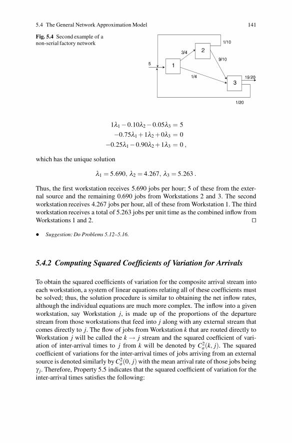
5.4 The General Network Approximation Model 141
Fig. 5.4 Second example of anon-serial factory network
1λ1 −0.10λ2−0.05λ3 = 5
−0.75λ1 +1λ2 +0λ3 = 0
−0.25λ1−0.90λ2 +1λ3 = 0 ,
which has the unique solution
λ1 = 5.690, λ2 = 4.267, λ3 = 5.263 .
Thus, the first workstation receives 5.690 jobs per hour; 5 of these from the exter-nal source and the remaining 0.690 jobs from Workstations 2 and 3. The secondworkstation receives 4.267 jobs per hour, all of these from Workstation 1. The thirdworkstation receives a total of 5.263 jobs per unit time as the combined inflow fromWorkstations 1 and 2. ��
• Suggestion: Do Problems 5.12–5.16.
5.4.2 Computing Squared Coefficients of Variation for Arrivals
To obtain the squared coefficients of variation for the composite arrival stream intoeach workstation, a system of linear equations relating all of these coefficients mustbe solved; thus, the solution procedure is similar to obtaining the net inflow rates,although the individual equations are much more complex. The inflow into a givenworkstation, say Workstation j, is made up of the proportions of the departurestream from those workstations that feed into j along with any external stream thatcomes directly to j. The flow of jobs from Workstation k that are routed directly toWorkstation j will be called the k → j stream and the squared coefficient of vari-ation of inter-arrival times to j from k will be denoted by C2
a(k, j). The squaredcoefficient of variations for the inter-arrival times of jobs arriving from an externalsource is denoted similarly by C2
a(0, j) with the mean arrival rate of those jobs beingγ j. Therefore, Property 5.5 indicates that the squared coefficient of variation for theinter-arrival times satisfies the following:

142 5 Multiple-Stage Single-Product Factory Models
C2a( j) =
γ j
λ jC2
a(0, j)+n
∑k=1
λk pk, j
λ jC2
a(k, j) , (5.5)
where P is the routing matrix and the mean rates, λi, come from Property 5.7. (Fre-quently, γ j = 0 and this component has no contribution.) Property 5.6 gives therelationship between departures and arrivals so that (5.5) is rewritten as
C2a( j) =
γ j
λ jC2
a(0, j)+n
∑k=1
λk pk, j
λ j
(
pk, jC2d(k)+1− pk, j
)
. (5.6)
The above system of equations involves both arrival stream and departure streamcharacterizations; thus, the final step is to express the departure streams in terms ofthe arrival streams using Property 5.2 and substitute this back into (5.6). You shouldbe able to show that the resulting system of equations is as follows:
Property 5.8. Consider a general network of n workstations with switchingrule defined by the routing matrix P and assume that the sum of at leastone row of P is strictly less than one. The characteristics of the flow of ex-ternal jobs to Workstation j are given by γ j and C2
a(0, j). The total meanrate of jobs coming into Workstation j is given by λ j (from Property 5.7)and the workstation consists of c j servers processing one job at-a-time. Eachserver within Workstation j has a mean service time of E[Tj] and squared co-efficient of variation for service of C2
s ( j) with workstation utilization factoru j = E[Tj]λ j/c j < 1. The values of C2
a( j) for j = 1, · · · ,n that satisfy
C2a( j) =
γ j
λ jC2
a(0, j)+n
∑k=1
λk pk, j
λ j
[
pk, j(1−u2k)C
2a(k)
+ pk, j u2k
(
C2s (k)+
√ck −1
√ck
)
+1− pk, j
]
for j = 1, · · · ,n
are the squared coefficients of variation for the inter-arrival times of jobsentering the various workstations.
Because the formula for determining the squared coefficient of variation of mergingarrival streams is an approximation and in some cases the formula for the squaredcoefficient of variation for inter-departure times is an approximation, the terms ob-tained from Property 5.8 are approximations. The system of equations given by theproperty can be solved fairly rapidly by an iterative procedure known as successivesubstitution. The idea is to initialize the C2
a(i) terms at some arbitrary value, say 1.0,and then use these values in the right-hand side of the system in Property 5.8 whichwill yield new values for the C2
a(i) terms. After the new values are obtained, thesenew values are used for the next iteration for the right-hand side of the equationsagain to obtain new values. This is repeated several times until the new values ob-tained on the left-hand side are equal (within some specified degree of accuracy) to
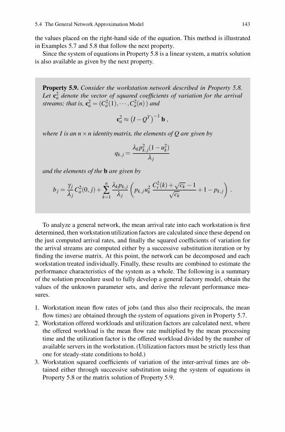
5.4 The General Network Approximation Model 143
the values placed on the right-hand side of the equation. This method is illustratedin Examples 5.7 and 5.8 that follow the next property.
Since the system of equations in Property 5.8 is a linear system, a matrix solutionis also available as given by the next property.
Property 5.9. Consider the workstation network described in Property 5.8.Let c2
a denote the vector of squared coefficients of variation for the arrivalstreams; that is, c2
a = (C2a(1), · · · ,C2
a(n) ) and
c2a ≈(
I −QT)−1
b ,
where I is an n×n identity matrix, the elements of Q are given by
qk, j =λk p2
k, j(1−u2k)
λ j
and the elements of the b are given by
b j =γ j
λ jC2
a(0, j)+n
∑k=1
λk pk, j
λ j
(
pk, j u2k
C2s (k)+
√ck −1
√ck
+1− pk, j
)
.
To analyze a general network, the mean arrival rate into each workstation is firstdetermined, then workstation utilization factors are calculated since these depend onthe just computed arrival rates, and finally the squared coefficients of variation forthe arrival streams are computed either by a successive substitution iteration or byfinding the inverse matrix. At this point, the network can be decomposed and eachworkstation treated individually. Finally, these results are combined to estimate theperformance characteristics of the system as a whole. The following is a summaryof the solution procedure used to fully develop a general factory model, obtain thevalues of the unknown parameter sets, and derive the relevant performance mea-sures.
1. Workstation mean flow rates of jobs (and thus also their reciprocals, the meanflow times) are obtained through the system of equations given in Property 5.7.
2. Workstation offered workloads and utilization factors are calculated next, wherethe offered workload is the mean flow rate multiplied by the mean processingtime and the utilization factor is the offered workload divided by the number ofavailable servers in the workstation. (Utilization factors must be strictly less thanone for steady-state conditions to hold.)
3. Workstation squared coefficients of variation of the inter-arrival times are ob-tained either through successive substitution using the system of equations inProperty 5.8 or the matrix solution of Property 5.9.

144 5 Multiple-Stage Single-Product Factory Models
Fig. 5.5 Factory topologyused in Example 5.7
4. The decomposition principle is used to obtain the mean time spent in the queueat each workstation using either Property 3.3 or 3.6. The mean service time isadded to the time in queue to obtain the mean workstation cycle time and thenLittle’s Law (Property 2.1) is used to obtain workstation W IP.
5. Factory W IP is obtained by summing the individual workstation W IPs, then thetotal mean cycle time for a job within the factory is derived from the applicationof Little’s Law again. Factory throughput is merely the sum of the external in-flows into the system, under the assumption of the existence of steady-state andno turning away of jobs.
This analysis process is illustrated with two examples starting with a systemof single server workstations, each processing a single job at a time. The secondexample has a mixture of single and multiple server workstations.
Example 5.7. Consider a factory that consists entirely of single-server workstationswith service time data for each workstation given by Table 5.3. Arrivals from an
Table 5.3 Workstation characteristics for Example 5.7
Workstation i E [Ts(i)] C2s (i)
1 7.80 min 1.03552 7.80 min 1.77513 9.60 min 0.39064 3.84 min 2.4414
external source enter into the factory at the first workstation, and the arrivals are ex-ponentially distributed with a mean rate of 5 jobs per hour. After initial processing,2/3 of the jobs are sent to Workstation 2 and 1/3 are sent to Workstation 3. After thesecond step of processing, jobs are tested at Workstation 4, and only 40% of the jobsare found to be acceptable. Ten percent of the completed jobs fail the testing com-pletely and are scrapped, at which time a new job is started to replace the scrappedjobs. Fifty percent of the jobs partially fail the testing and can be reworked. Sixtypercent of the partial failures are sent to Workstation 3 and the others are sent toWorkstation 2. After reworking, the jobs are sent again for testing at Workstation4 with the same percentage of passing, partially failing, and completely failing thetesting. (Figure 5.5 illustrates these job flows and switching probabilities.)
Management is interested in the mean cycle time for jobs, factory inventory lev-els, and workloads at each workstation. To answer these questions, each of the five
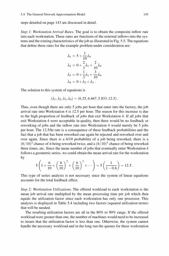
5.4 The General Network Approximation Model 145
steps detailed on page 143 are discussed in detail.
Step 1: Workstation Arrival Rates. The goal is to obtain the composite inflow rateinto each workstation. These rates are functions of the external inflows into the sys-tems and the routing characteristics of the job as illustrated in Fig. 5.5. The equationsthat define these rates for the example problem under consideration are:
λ1 = 5 +1
10λ4
λ2 = 0 +23
λ1 +210
λ4
λ3 = 0 +13
λ1 +310
λ4
λ4 = 0 +λ2 +λ3 .
The solution to this system of equations is
(λ1,λ2,λ3,λ4) = (6.25,6.667,5.833,12.5) .
Thus, even though there are only 5 jobs per hour that enter into the factory, the jobarrival rate into Workstation 4 is 12.5 per hour. The reason for this increase is dueto the high proportion of feedback of jobs that exit Workstation 4. If all jobs thatexit Workstation 4 were acceptable in quality, then there would be no feedback orreworking of jobs and the inflow rate into Workstation 4 would merely be 5 jobsper hour. The 12.5/hr rate is a consequence of these feedback probabilities and thefact that a job that has been reworked can again be rejected and reworked over andover again. Since there is a 6/10 probability of a job being reworked, there is a(6/10)2 chance of it being reworked twice, and a (6/10)3 chance of being reworkedthree times, etc. Since the mean number of jobs that eventually enter Workstation 4follows a geometric series, we could obtain the mean arrival rate for the workstationby
5
(
1 +610
+(
610
)2
+(
610
)3
+ · · ·)
= 5
(
11−0.6
)
= 12.5 .
This type of series analysis is not necessary since the system of linear equationsaccounts for the total feedback effect.
Step 2: Workstation Utilizations. The offered workload to each workstation is themean job arrival rate multiplied by the mean processing time per job which thenequals the utilization factor since each workstation has only one processor. Thisanalysis is displayed in Table 5.4 including two factors (squared utilization terms)that will be needed.
The resulting utilization factors are all in the 80% to 90% range. If the offeredworkload were greater than one, the number of machines would need to be increasedto insure that the utilization factor is less than one. Otherwise, the system cannothandle the necessary workload and in the long run the queues for these workstation
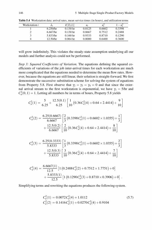
146 5 Multiple-Stage Single-Product Factory Models
Table 5.4 Workstation data: arrival rates, mean service times (in hours), and utilization terms
Workstation i λi E [Ts(i)] ui u2i 1−u2
i1 6.250/hr 0.130 hr 0.8125 0.6602 0.33982 6.667/hr 0.130 hr 0.8667 0.7512 0.24883 5.833/hr 0.160 hr 0.9333 0.8710 0.12904 12.50/hr 0.064 hr 0.8000 0.6400 0.3600
will grow indefinitely. This violates the steady-state assumption underlying all ourmodels and further analysis could not be performed.
Step 3: Squared Coefficients of Variation. The equations defining the squared co-efficients of variations of the job inter-arrival times for each workstation are muchmore complicated that the equations needed to determine the mean flow rates. How-ever, because the equations are still linear, their solution is straight-forward. We firstdemonstrate the successive substitution scheme for solving the system of equationsfrom Property 5.8. First observe that γ2 = γ3 = γ4 = 0 and that since the exter-nal arrival stream to the first workstation is exponential, we have γ1 = 5/hr andC2
a(0,1) = 1. Letting all numbers be in terms of hours, Property 5.8 yields
C2a(1) =
56.25
+12.5(0.1)
6.25
[
110
(
0.36C2a(4)+0.64×2.4414
)
+9
10
]
C2a(2) =
6.25(0.6667)6.6667
[
23
(
0.3398C2a(1)+0.6602×1.0355
)
+13
]
+12.5(0.2)
6.6667
[
210
(
0.36C2a(4)+0.64×2.4414
)
+8
10
]
C2a(3) =
6.25(0.3333)5.8333
[
13
(
0.3398C2a(1)+0.6602×1.0355
)
+23
]
+12.5(0.3)
5.8333
[
310
(
0.36C2a(4)+0.64×2.4414
)
+7
10
]
C2a(4) =
6.6667(1)12.5
[
1(
0.2488C2a(2)+0.7512×1.7751
)
+0]
+5.8333(1)
12.5
[
1(
0.1290C2a(3)+0.8710×0.3906
)
+0]
.
Simplifying terms and rewriting the equations produces the following system.
C2a(1) = 0.0072C2
a(4)+1.0112 (5.7)
C2a(2) = 0.1416C2
a(1)+0.0270C2a(4)+0.9104
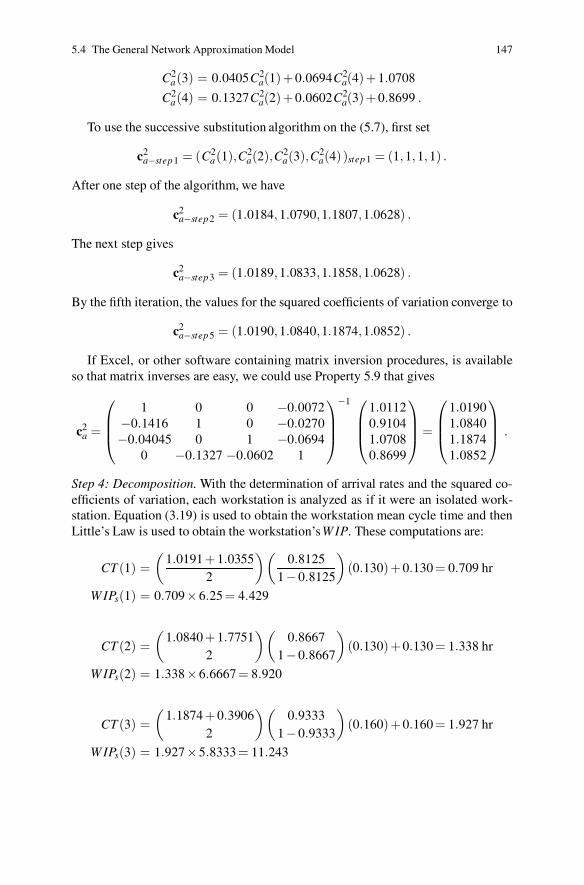
5.4 The General Network Approximation Model 147
C2a(3) = 0.0405C2
a(1)+0.0694C2a(4)+1.0708
C2a(4) = 0.1327C2
a(2)+0.0602C2a(3)+0.8699 .
To use the successive substitution algorithm on the (5.7), first set
c2a−step1 = (C2
a(1),C2a(2),C2
a(3),C2a(4) )step1 = (1,1,1,1) .
After one step of the algorithm, we have
c2a−step2 = (1.0184,1.0790,1.1807,1.0628) .
The next step gives
c2a−step3 = (1.0189,1.0833,1.1858,1.0628) .
By the fifth iteration, the values for the squared coefficients of variation converge to
c2a−step5 = (1.0190,1.0840,1.1874,1.0852) .
If Excel, or other software containing matrix inversion procedures, is availableso that matrix inverses are easy, we could use Property 5.9 that gives
c2a =
⎛
⎜
⎜
⎝
1 0 0 −0.0072−0.1416 1 0 −0.0270−0.04045 0 1 −0.0694
0 −0.1327 −0.0602 1
⎞
⎟
⎟
⎠
−1 ⎛
⎜
⎜
⎝
1.01120.91041.07080.8699
⎞
⎟
⎟
⎠
=
⎛
⎜
⎜
⎝
1.01901.08401.18741.0852
⎞
⎟
⎟
⎠
.
Step 4: Decomposition. With the determination of arrival rates and the squared co-efficients of variation, each workstation is analyzed as if it were an isolated work-station. Equation (3.19) is used to obtain the workstation mean cycle time and thenLittle’s Law is used to obtain the workstation’sW IP. These computations are:
CT (1) =(
1.0191 +1.03552
)(
0.81251−0.8125
)
(0.130)+0.130 = 0.709 hr
W IPs(1) = 0.709×6.25 = 4.429
CT (2) =(
1.0840 +1.77512
)(
0.86671−0.8667
)
(0.130)+0.130 = 1.338 hr
W IPs(2) = 1.338×6.6667 = 8.920
CT (3) =(
1.1874 +0.39062
)(
0.93331−0.9333
)
(0.160)+0.160 = 1.927 hr
W IPs(3) = 1.927×5.8333 = 11.243
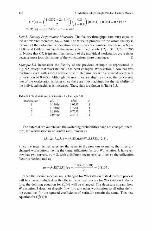
148 5 Multiple-Stage Single-Product Factory Models
CT (4) =(
1.0852 +2.44142
)(
0.81−0.8
)
(0.064)+0.064 = 0.515 hr
W IPs(4) = 0.5154×12.5 = 6.443 .
Step 5: Factory Performance Measures. The factory throughput rate must equal tothe inflow rate; therefore, ths = 5/hr. The work-in-process for the whole factory isthe sum of the individual workstation work-in-process numbers; therefore, WIPs =31.03, and Little’s Law yields the mean cycle time; namely, CTs = 31.03/5 = 6.206hr. Notice that CTs is greater than the sum of the individual workstation cycle timesbecause most jobs visit some of the workstations more than once. ��
Example 5.8. Reconsider the factory of the previous example as represented inFig. 5.5 except that Workstation 3 has been changed. Workstation 3 now has twomachines, each with a mean service time of 16.8 minutes with a squared coefficientof variation of 0.7653. Although the machines are slightly slower, the processingrate of the workstation is faster since there are two machines but the variability ofthe individual machines is increased. These data are shown in Table 5.5.
Table 5.5 Workstation characteristics for Example 5.8
Workstation i E [Ts(i)] C2s (i) ci
1 0.130 hr 1.0355 12 0.130 hr 1.7751 13 0.280 hr 0.7653 24 0.064 hr 2.4414 1
The external arrival rate and the switching probabilities have not changed; there-fore, the workstation mean arrival rates remain as
(λ1,λ2,λ3,λ4) = (6.25,6.6667,5.8333,12.5) .
Since the mean arrival rates are the same in the previous example, the three un-changed workstations having the same utilization factors. Workstation 3, however,now has two servers, c3 = 2, with a different mean service times so the utilizationfactor is recalculated as
u3 = λ3E[Ts(3)]/c3 =5.8333(0.28)
2= 0.8167 .
Since the service mechanism is changed for Workstation 3, its departure processwill be changed which directly effects the arrival process for Workstation 4; there-fore, the defining equation for C2
a(4) will be changed. The departure stream fromWorkstation 3 does not directly flow into any other workstation so all other defin-ing equations for the squared coefficients of variation remain the same. This newequation for C2
a(4) is
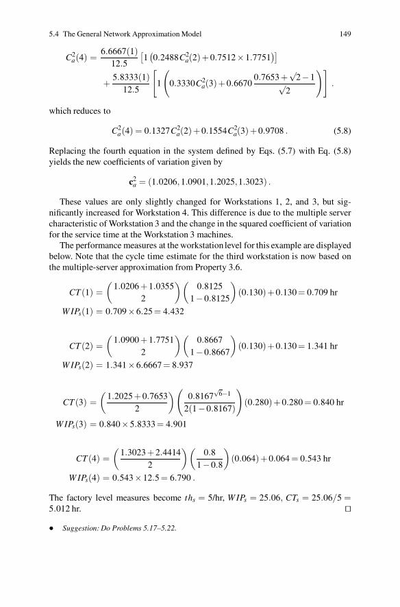
5.4 The General Network Approximation Model 149
C2a(4) =
6.6667(1)12.5
[
1(
0.2488C2a(2)+0.7512×1.7751
)]
+5.8333(1)
12.5
[
1
(
0.3330C2a(3)+0.6670
0.7653 +√
2−1√2
)]
.
which reduces to
C2a(4) = 0.1327C2
a(2)+0.1554C2a(3)+0.9708 . (5.8)
Replacing the fourth equation in the system defined by Eqs. (5.7) with Eq. (5.8)yields the new coefficients of variation given by
c2a = (1.0206,1.0901,1.2025,1.3023) .
These values are only slightly changed for Workstations 1, 2, and 3, but sig-nificantly increased for Workstation 4. This difference is due to the multiple servercharacteristic of Workstation 3 and the change in the squared coefficient of variationfor the service time at the Workstation 3 machines.
The performance measures at the workstation level for this example are displayedbelow. Note that the cycle time estimate for the third workstation is now based onthe multiple-server approximation from Property 3.6.
CT (1) =(
1.0206 +1.03552
)(
0.81251−0.8125
)
(0.130)+0.130 = 0.709 hr
W IPs(1) = 0.709×6.25 = 4.432
CT (2) =(
1.0900 +1.77512
)(
0.86671−0.8667
)
(0.130)+0.130 = 1.341 hr
W IPs(2) = 1.341×6.6667 = 8.937
CT (3) =(
1.2025 +0.76532
)
(
0.8167√
6−1
2(1−0.8167)
)
(0.280)+0.280 = 0.840 hr
W IPs(3) = 0.840×5.8333 = 4.901
CT (4) =(
1.3023 +2.44142
)(
0.81−0.8
)
(0.064)+0.064 = 0.543 hr
W IPs(4) = 0.543×12.5 = 6.790 .
The factory level measures become ths = 5/hr, W IPs = 25.06, CTs = 25.06/5 =5.012 hr. ��
• Suggestion: Do Problems 5.17–5.22.
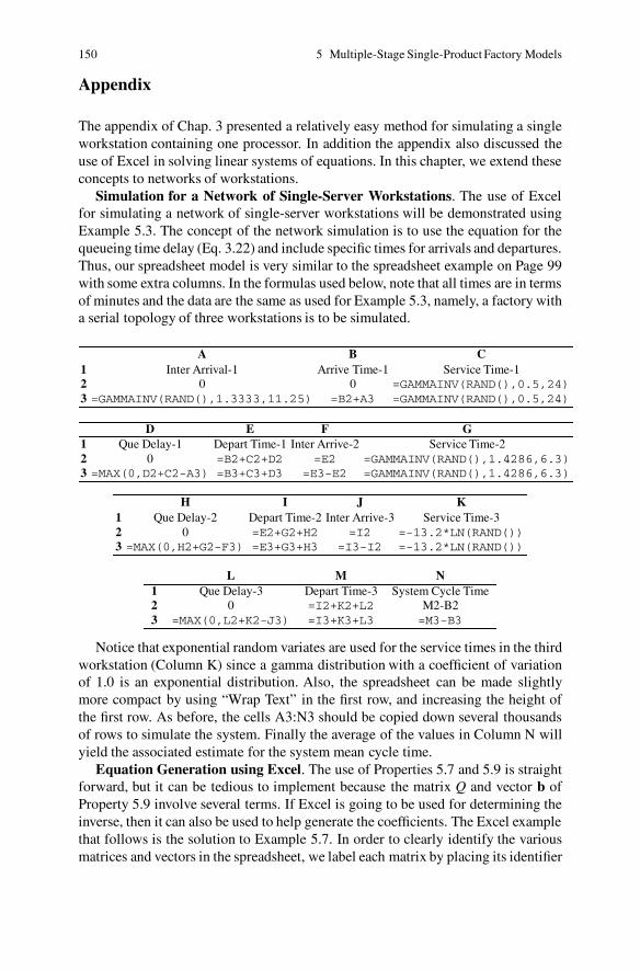
150 5 Multiple-Stage Single-Product Factory Models
Appendix
The appendix of Chap. 3 presented a relatively easy method for simulating a singleworkstation containing one processor. In addition the appendix also discussed theuse of Excel in solving linear systems of equations. In this chapter, we extend theseconcepts to networks of workstations.
Simulation for a Network of Single-Server Workstations. The use of Excelfor simulating a network of single-server workstations will be demonstrated usingExample 5.3. The concept of the network simulation is to use the equation for thequeueing time delay (Eq. 3.22) and include specific times for arrivals and departures.Thus, our spreadsheet model is very similar to the spreadsheet example on Page 99with some extra columns. In the formulas used below, note that all times are in termsof minutes and the data are the same as used for Example 5.3, namely, a factory witha serial topology of three workstations is to be simulated.
A B C1 Inter Arrival-1 Arrive Time-1 Service Time-12 0 0 =GAMMAINV(RAND(),0.5,24)3 =GAMMAINV(RAND(),1.3333,11.25) =B2+A3 =GAMMAINV(RAND(),0.5,24)
D E F G1 Que Delay-1 Depart Time-1 Inter Arrive-2 Service Time-22 0 =B2+C2+D2 =E2 =GAMMAINV(RAND(),1.4286,6.3)3 =MAX(0,D2+C2-A3) =B3+C3+D3 =E3-E2 =GAMMAINV(RAND(),1.4286,6.3)
H I J K1 Que Delay-2 Depart Time-2 Inter Arrive-3 Service Time-32 0 =E2+G2+H2 =I2 =-13.2*LN(RAND())3 =MAX(0,H2+G2-F3) =E3+G3+H3 =I3-I2 =-13.2*LN(RAND())
L M N1 Que Delay-3 Depart Time-3 System Cycle Time2 0 =I2+K2+L2 M2-B23 =MAX(0,L2+K2-J3) =I3+K3+L3 =M3-B3
Notice that exponential random variates are used for the service times in the thirdworkstation (Column K) since a gamma distribution with a coefficient of variationof 1.0 is an exponential distribution. Also, the spreadsheet can be made slightlymore compact by using “Wrap Text” in the first row, and increasing the height ofthe first row. As before, the cells A3:N3 should be copied down several thousandsof rows to simulate the system. Finally the average of the values in Column N willyield the associated estimate for the system mean cycle time.
Equation Generation using Excel. The use of Properties 5.7 and 5.9 is straightforward, but it can be tedious to implement because the matrix Q and vector b ofProperty 5.9 involve several terms. If Excel is going to be used for determining theinverse, then it can also be used to help generate the coefficients. The Excel examplethat follows is the solution to Example 5.7. In order to clearly identify the variousmatrices and vectors in the spreadsheet, we label each matrix by placing its identifier
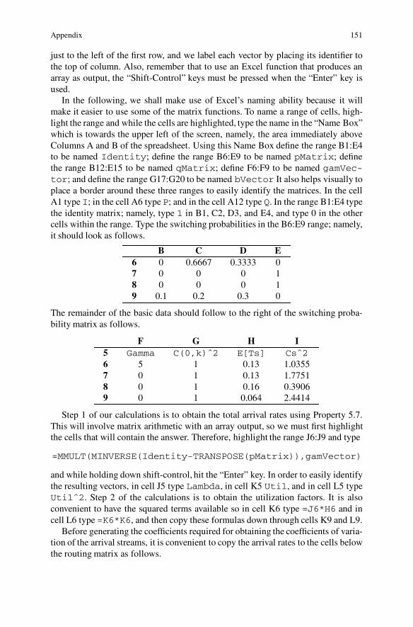
Appendix 151
just to the left of the first row, and we label each vector by placing its identifier tothe top of column. Also, remember that to use an Excel function that produces anarray as output, the “Shift-Control” keys must be pressed when the “Enter” key isused.
In the following, we shall make use of Excel’s naming ability because it willmake it easier to use some of the matrix functions. To name a range of cells, high-light the range and while the cells are highlighted, type the name in the “Name Box”which is towards the upper left of the screen, namely, the area immediately aboveColumns A and B of the spreadsheet. Using this Name Box define the range B1:E4to be named Identity; define the range B6:E9 to be named pMatrix; definethe range B12:E15 to be named qMatrix; define F6:F9 to be named gamVec-tor; and define the range G17:G20 to be named bVector It also helps visually toplace a border around these three ranges to easily identify the matrices. In the cellA1 type I; in the cell A6 type P; and in the cell A12 type Q. In the range B1:E4 typethe identity matrix; namely, type 1 in B1, C2, D3, and E4, and type 0 in the othercells within the range. Type the switching probabilities in the B6:E9 range; namely,it should look as follows.
B C D E6 0 0.6667 0.3333 07 0 0 0 18 0 0 0 19 0.1 0.2 0.3 0
The remainder of the basic data should follow to the right of the switching proba-bility matrix as follows.
F G H I5 Gamma C(0,k)ˆ2 E[Ts] Csˆ26 5 1 0.13 1.03557 0 1 0.13 1.77518 0 1 0.16 0.39069 0 1 0.064 2.4414
Step 1 of our calculations is to obtain the total arrival rates using Property 5.7.This will involve matrix arithmetic with an array output, so we must first highlightthe cells that will contain the answer. Therefore, highlight the range J6:J9 and type
=MMULT(MINVERSE(Identity-TRANSPOSE(pMatrix)),gamVector)
and while holding down shift-control, hit the “Enter” key. In order to easily identifythe resulting vectors, in cell J5 type Lambda, in cell K5 Util, and in cell L5 typeUtilˆ2. Step 2 of the calculations is to obtain the utilization factors. It is alsoconvenient to have the squared terms available so in cell K6 type =J6*H6 and incell L6 type =K6*K6, and then copy these formulas down through cells K9 and L9.
Before generating the coefficients required for obtaining the coefficients of varia-tion of the arrival streams, it is convenient to copy the arrival rates to the cells belowthe routing matrix as follows.
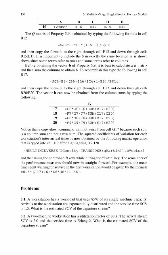
152 5 Multiple-Stage Single-Product Factory Models
A B C D E10 Lambda =J6 =J7 =J8 =J9
The Q matrix of Property 5.9 is obtained by typing the following formula in cellB12
=$J6*B6*B6*(1-$L6)/B$10
and then copy the formula to the right through cell E12 and down through cellsB15:E15. It is important to include the $ in exactly the same location as is shownabove since some terms refer to rows and some terms refer to columns.
Before obtaining the vector b of Property 5.9, it is best to calculate a B matrixand then sum the columns to obtain b. To accomplish this type the following in cellB17.
=$J6*B6*(B6*$L6*$I6+1-B6)/B$10
and then copy the formula to the right through cell E17 and down through cellsB20:E20. The vector b can now be obtained from the column sums by typing thefollowing:
G17 =F6*G6/J6+SUM(B17:B20)18 =F7*G7/J7+SUM(C17:C20)19 =F8*G8/J8+SUM(D17:D20)20 =F9*G9/J9+SUM(E17:E20)
Notice that a copy-down command will not work from cell G17 because each sumis a column sum and not a row sum. The squared coefficients of variation for eachworkstation’s inter-arrival times is now obtained by the following matrix operationthat is typed into cell J17 after highlighting J17:J20
=MMULT(MINVERSE(Identity-TRANSPOSE(qMartix)),bVector)
and then using the control-shift keys while hitting the “Enter” key. The remainder ofthe performance measures should now be straight-forward. For example, the meantime spent waiting for service in the first workstation would be given by the formula=0.5*(J17+I6)*K6*H6/(1-K6).
Problems
5.1. A workstation has a workload that uses 85% of its single machine capacity.Arrivals to the workstation are exponentially distributed and the service time SCVis 1.5. What is the estimated SCV of the departure stream?
5.2. A two-machine workstation has a utilization factor of 80%. The arrival streamSCV is 2.0 and the service time is Erlang-2. What is the estimated SCV of thedeparture stream?
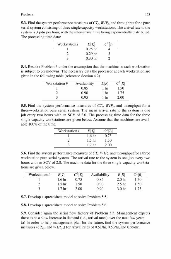
Problems 153
5.3. Find the system performance measures of CTs, W IPs, and throughput for a pureserial system consisting of three single capacity workstations. The arrival rate to thesystem is 3 jobs per hour, with the inter-arrival time being exponentially distributed.The processing time data:
Workstation i E[Ti] C2[Ti]1 0.25 hr 42 0.29 hr 33 0.30 hr 2
5.4. Resolve Problem 3 under the assumption that the machine in each workstationis subject to breakdowns. The necessary data the processor at each workstation aregiven in the following table (reference Section 4.2).
Workstation # Availability E[R] C2[R]1 0.85 1 hr 1.502 0.90 1 hr 1.753 0.95 1 hr 2.00
5.5. Find the system performance measures of CTs, WIPs, and throughput for athree-workstation pure serial system. The mean arrival rate to the system is onejob every two hours with an SCV of 2.0. The processing time data for the threesingle-capacity workstations are given below. Assume that the machines are avail-able 100% of the time.
Workstation i E[Ti] C2[Ti]1 1.6 hr 0.752 1.5 hr 1.503 1.7 hr 2.00
5.6. Find the system performance measures of CTs, W IPs, and throughput for a threeworkstation pure serial system. The arrival rate to the system is one job every twohours with an SCV of 2.0. The machine data for the three single-capacity worksta-tions are given below.
Workstation i E[Ti] C2[Ti] Availability E[R] C2[R]1 1.6 hr 0.75 0.85 2.0 hr 1.302 1.5 hr 1.50 0.90 2.5 hr 1.503 1.7 hr 2.00 0.90 3.0 hr 1.75
5.7. Develop a spreadsheet model to solve Problem 5.5.
5.8. Develop a spreadsheet model to solve Problem 5.6.
5.9. Consider again the serial flow factory of Problem 5.5. Management expectsthere to be a slow increase in demand (i.e., arrival rates) over the next few years.(a) In order to help management plan for the future, find the system performancemeasures (CTsys and W IPsys) for arrival rates of 0.51/hr, 0.53/hr, and 0.55/hr.
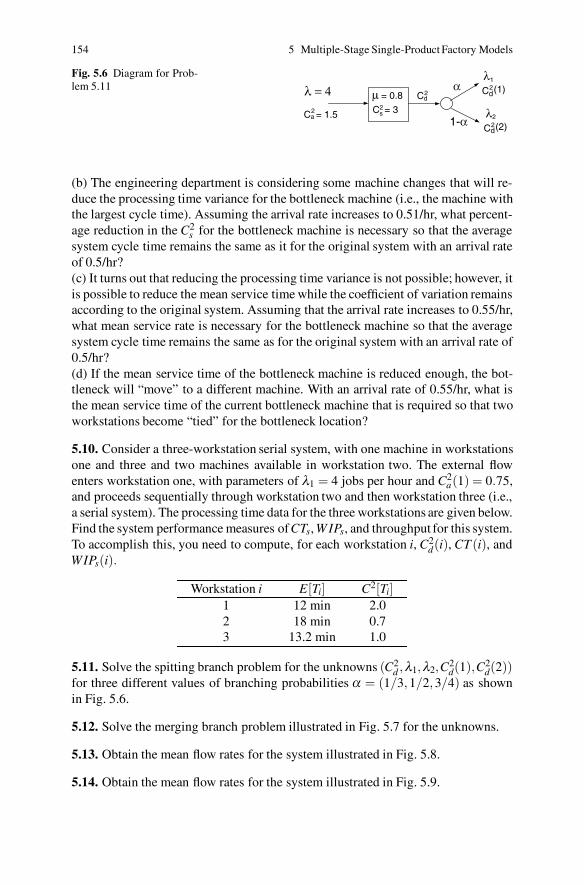
154 5 Multiple-Stage Single-Product Factory Models
Fig. 5.6 Diagram for Prob-lem 5.11
μ = 0.8
Cs = 32Ca = 1.52
Cd2 Cd
2(1)λ1
λ2
Cd2(2)
α
1-α
λ = 4
(b) The engineering department is considering some machine changes that will re-duce the processing time variance for the bottleneck machine (i.e., the machine withthe largest cycle time). Assuming the arrival rate increases to 0.51/hr, what percent-age reduction in the C2
s for the bottleneck machine is necessary so that the averagesystem cycle time remains the same as it for the original system with an arrival rateof 0.5/hr?(c) It turns out that reducing the processing time variance is not possible; however, itis possible to reduce the mean service time while the coefficient of variation remainsaccording to the original system. Assuming that the arrival rate increases to 0.55/hr,what mean service rate is necessary for the bottleneck machine so that the averagesystem cycle time remains the same as for the original system with an arrival rate of0.5/hr?(d) If the mean service time of the bottleneck machine is reduced enough, the bot-tleneck will “move” to a different machine. With an arrival rate of 0.55/hr, what isthe mean service time of the current bottleneck machine that is required so that twoworkstations become “tied” for the bottleneck location?
5.10. Consider a three-workstation serial system, with one machine in workstationsone and three and two machines available in workstation two. The external flowenters workstation one, with parameters of λ1 = 4 jobs per hour and C2
a(1) = 0.75,and proceeds sequentially through workstation two and then workstation three (i.e.,a serial system). The processing time data for the three workstations are given below.Find the system performance measures ofCTs, W IPs, and throughput for this system.To accomplish this, you need to compute, for each workstation i, C2
d(i), CT (i), andWIPs(i).
Workstation i E[Ti] C2[Ti]1 12 min 2.02 18 min 0.73 13.2 min 1.0
5.11. Solve the spitting branch problem for the unknowns (C2d ,λ1,λ2,C2
d(1),C2d(2))
for three different values of branching probabilities α = (1/3,1/2,3/4) as shownin Fig. 5.6.
5.12. Solve the merging branch problem illustrated in Fig. 5.7 for the unknowns.
5.13. Obtain the mean flow rates for the system illustrated in Fig. 5.8.
5.14. Obtain the mean flow rates for the system illustrated in Fig. 5.9.
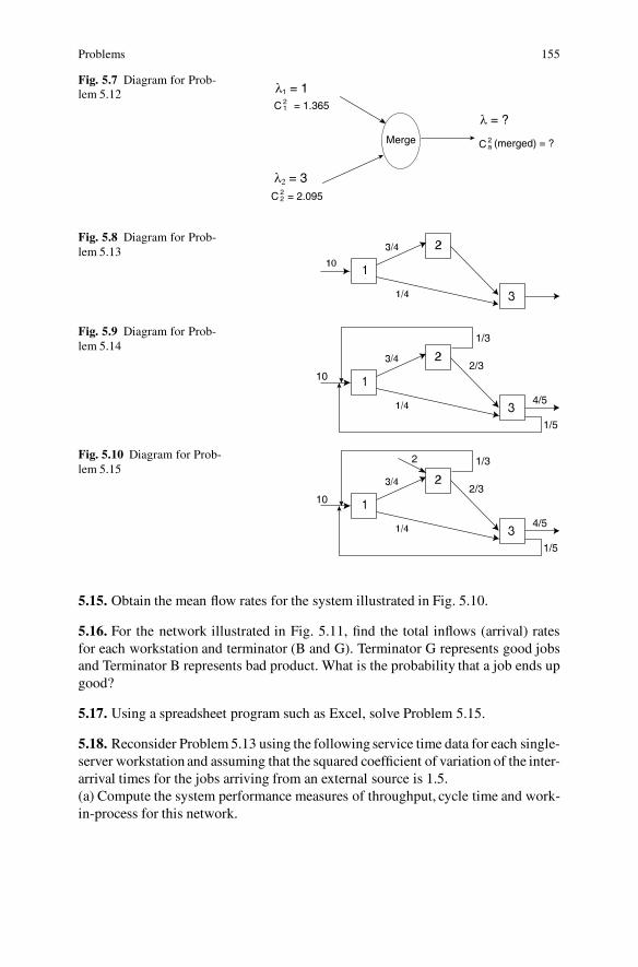
Problems 155
Fig. 5.7 Diagram for Prob-lem 5.12
C 2a (merged) = ?
C 21 = 1.365
C 22 = 2.095
Merge
λ1 = 1
λ2 = 3
λ = ?
Fig. 5.8 Diagram for Prob-lem 5.13
Fig. 5.9 Diagram for Prob-lem 5.14
2/3
4/5
1/5
1/3
10
Fig. 5.10 Diagram for Prob-lem 5.15
2/3
4/5
1/5
1/32
10
5.15. Obtain the mean flow rates for the system illustrated in Fig. 5.10.
5.16. For the network illustrated in Fig. 5.11, find the total inflows (arrival) ratesfor each workstation and terminator (B and G). Terminator G represents good jobsand Terminator B represents bad product. What is the probability that a job ends upgood?
5.17. Using a spreadsheet program such as Excel, solve Problem 5.15.
5.18. Reconsider Problem 5.13 using the following service time data for each single-server workstation and assuming that the squared coefficient of variation of the inter-arrival times for the jobs arriving from an external source is 1.5.(a) Compute the system performance measures of throughput, cycle time and work-in-process for this network.
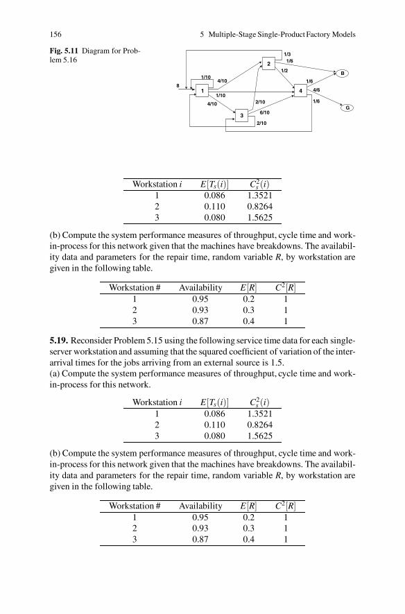
156 5 Multiple-Stage Single-Product Factory Models
Fig. 5.11 Diagram for Prob-lem 5.16
1
2
3
4
B
G
8
1/104/10
4/10
1/10
1/31/6
1/2
2/10
6/10
2/10
1/6
4/6
1/6
Workstation i E[Ts(i)] C2s (i)
1 0.086 1.35212 0.110 0.82643 0.080 1.5625
(b) Compute the system performance measures of throughput, cycle time and work-in-process for this network given that the machines have breakdowns. The availabil-ity data and parameters for the repair time, random variable R, by workstation aregiven in the following table.
Workstation # Availability E[R] C2[R]1 0.95 0.2 12 0.93 0.3 13 0.87 0.4 1
5.19. Reconsider Problem 5.15 using the following service time data for each single-server workstation and assuming that the squared coefficient of variation of the inter-arrival times for the jobs arriving from an external source is 1.5.(a) Compute the system performance measures of throughput, cycle time and work-in-process for this network.
Workstation i E[Ts(i)] C2s (i)
1 0.086 1.35212 0.110 0.82643 0.080 1.5625
(b) Compute the system performance measures of throughput, cycle time and work-in-process for this network given that the machines have breakdowns. The availabil-ity data and parameters for the repair time, random variable R, by workstation aregiven in the following table.
Workstation # Availability E[R] C2[R]1 0.95 0.2 12 0.93 0.3 13 0.87 0.4 1
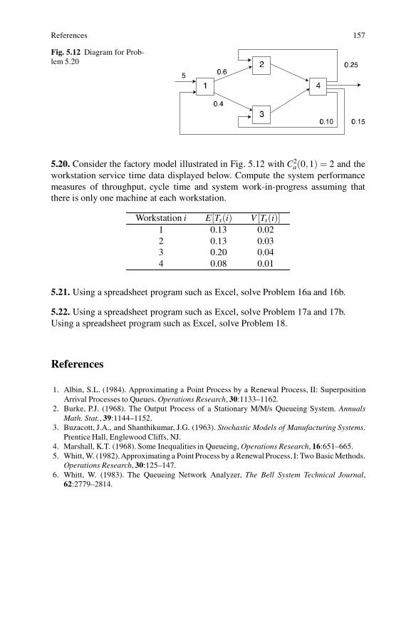
References 157
Fig. 5.12 Diagram for Prob-lem 5.20
5.20. Consider the factory model illustrated in Fig. 5.12 with C2a(0,1) = 2 and the
workstation service time data displayed below. Compute the system performancemeasures of throughput, cycle time and system work-in-progress assuming thatthere is only one machine at each workstation.
Workstation i E[Ts(i) V [Ts(i)]1 0.13 0.022 0.13 0.033 0.20 0.044 0.08 0.01
5.21. Using a spreadsheet program such as Excel, solve Problem 16a and 16b.
5.22. Using a spreadsheet program such as Excel, solve Problem 17a and 17b.Using a spreadsheet program such as Excel, solve Problem 18.
References
1. Albin, S.L. (1984). Approximating a Point Process by a Renewal Process, II: SuperpositionArrival Processes to Queues. Operations Research, 30:1133–1162.
2. Burke, P.J. (1968). The Output Process of a Stationary M/M/s Queueing System. AnnualsMath. Stat., 39:1144–1152.
3. Buzacott, J.A., and Shanthikumar, J.G. (1963). Stochastic Models of Manufacturing Systems.Prentice Hall, Englewood Cliffs, NJ.
4. Marshall, K.T. (1968). Some Inequalities in Queueing, Operations Research, 16:651–665.5. Whitt, W. (1982).Approximating a Point Process by a Renewal Process, I: Two Basic Methods.
Operations Research, 30:125–147.6. Whitt, W. (1983). The Queueing Network Analyzer, The Bell System Technical Journal,
62:2779–2814.
Chapter 6Multiple Product Factory Models
Most manufacturing facilities are setup to produce more than a single product. Evenin the case of single product facilities, if the product visits a workstation morethan once with different processing times at each visit, then the workstation seesthe equivalent of multiple products. Such revisiting production schemes, called re-entrant flow systems, are prevalent in the semiconductor industry where it is notunusual for a product to be routed to the same machine group for distinct process-ing 20 or more times.
Modeling multiple product facilities is not significantly more difficult than singleproduct models. There are two basic principles to keep in mind. First, the workloadon a workstation is, as before, the sum of all the visits multiplied by the processingtime per visit. This concept was introduced in the previous chapter (see p. 143) andsince we use it in a more general setting here, we give a formal definition.
Definition 6.1. The offered workload (or simply the workload) of a workstation isthe total amount of work that is required of a workstation per unit of time. Theworkload is determined by the sum of the total arrival rate (per hour) for each prod-uct type multiplied by its associated mean processing time (in hours). For purposesof determining workload, when a specific product type revisits a workstation, it isconsidered as a separate product type.
The second basic principle is that job flow needs to be maintained by producttype. That is, the number of visits to each workstation by product class is needed.Different products can have different probabilistic flows through the production fa-cility as well as different processing time characteristics. Hence, the number of visitsto each workstation by product needs to be developed. This analysis requires the so-lution of a network flow system of equations by product. Here again as was done inthe preceding chapter, the processing time is assumed to follow the same distributionfor each product on each visit to a given workstation (of course due to randomness,the actual processing times will vary even though the distribution is the same). There-entrant flow situation with different processing distributions per visit requires adifferent modeling paradigm that is taken up in Sect. 6.5.
159
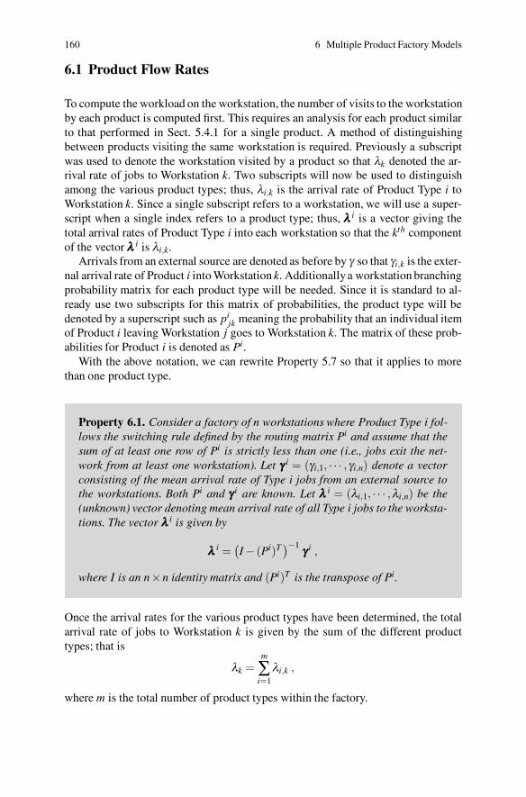
160 6 Multiple Product Factory Models
6.1 Product Flow Rates
To compute the workload on the workstation, the number of visits to the workstationby each product is computed first. This requires an analysis for each product similarto that performed in Sect. 5.4.1 for a single product. A method of distinguishingbetween products visiting the same workstation is required. Previously a subscriptwas used to denote the workstation visited by a product so that λk denoted the ar-rival rate of jobs to Workstation k. Two subscripts will now be used to distinguishamong the various product types; thus, λi,k is the arrival rate of Product Type i toWorkstation k. Since a single subscript refers to a workstation, we will use a super-script when a single index refers to a product type; thus, λλλ i is a vector giving thetotal arrival rates of Product Type i into each workstation so that the kth componentof the vector λλλ i is λi,k.
Arrivals from an external source are denoted as before by γ so that γi,k is the exter-nal arrival rate of Product i into Workstation k. Additionally a workstation branchingprobability matrix for each product type will be needed. Since it is standard to al-ready use two subscripts for this matrix of probabilities, the product type will bedenoted by a superscript such as pi
jk meaning the probability that an individual itemof Product i leaving Workstation j goes to Workstation k. The matrix of these prob-abilities for Product i is denoted as Pi.
With the above notation, we can rewrite Property 5.7 so that it applies to morethan one product type.
Property 6.1. Consider a factory of n workstations where Product Type i fol-lows the switching rule defined by the routing matrix Pi and assume that thesum of at least one row of Pi is strictly less than one (i.e., jobs exit the net-work from at least one workstation). Let γγγ i = (γi,1, · · · , γi,n) denote a vectorconsisting of the mean arrival rate of Type i jobs from an external source tothe workstations. Both Pi and γγγ i are known. Let λλλ i = (λi,1, · · · ,λi,n) be the(unknown) vector denoting mean arrival rate of all Type i jobs to the worksta-tions. The vector λλλ i is given by
λλλ i =(
I − (Pi)T)−1 γγγ i ,
where I is an n×n identity matrix and (Pi)T is the transpose of Pi.
Once the arrival rates for the various product types have been determined, the totalarrival rate of jobs to Workstation k is given by the sum of the different producttypes; that is
λk =m
∑i=1
λi,k ,
where m is the total number of product types within the factory.
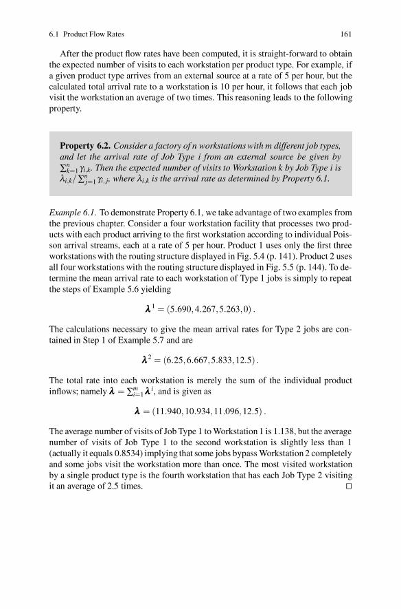
6.1 Product Flow Rates 161
After the product flow rates have been computed, it is straight-forward to obtainthe expected number of visits to each workstation per product type. For example, ifa given product type arrives from an external source at a rate of 5 per hour, but thecalculated total arrival rate to a workstation is 10 per hour, it follows that each jobvisit the workstation an average of two times. This reasoning leads to the followingproperty.
Property 6.2. Consider a factory of n workstations with m different job types,and let the arrival rate of Job Type i from an external source be given by∑n
k=1 γi,k. Then the expected number of visits to Workstation k by Job Type i isλi,k/∑n
j=1 γi, j, where λi,k is the arrival rate as determined by Property 6.1.
Example 6.1. To demonstrate Property 6.1, we take advantage of two examples fromthe previous chapter. Consider a four workstation facility that processes two prod-ucts with each product arriving to the first workstation according to individual Pois-son arrival streams, each at a rate of 5 per hour. Product 1 uses only the first threeworkstations with the routing structure displayed in Fig. 5.4 (p. 141). Product 2 usesall four workstations with the routing structure displayed in Fig. 5.5 (p. 144). To de-termine the mean arrival rate to each workstation of Type 1 jobs is simply to repeatthe steps of Example 5.6 yielding
λλλ 1 = (5.690,4.267,5.263,0) .
The calculations necessary to give the mean arrival rates for Type 2 jobs are con-tained in Step 1 of Example 5.7 and are
λλλ2 = (6.25,6.667,5.833,12.5) .
The total rate into each workstation is merely the sum of the individual productinflows; namely λλλ = ∑m
i=1 λλλ i, and is given as
λλλ = (11.940,10.934,11.096,12.5) .
The average number of visits of Job Type 1 to Workstation 1 is 1.138, but the averagenumber of visits of Job Type 1 to the second workstation is slightly less than 1(actually it equals 0.8534) implying that some jobs bypass Workstation 2 completelyand some jobs visit the workstation more than once. The most visited workstationby a single product type is the fourth workstation that has each Job Type 2 visitingit an average of 2.5 times. ��
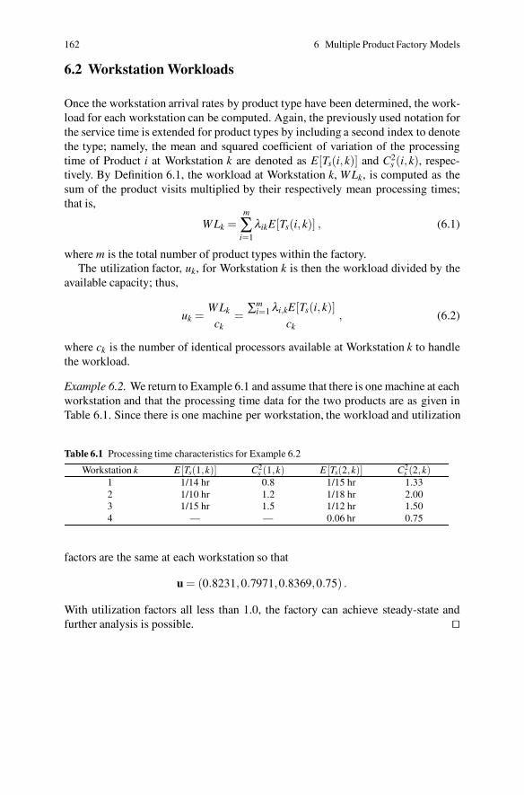
162 6 Multiple Product Factory Models
6.2 Workstation Workloads
Once the workstation arrival rates by product type have been determined, the work-load for each workstation can be computed. Again, the previously used notation forthe service time is extended for product types by including a second index to denotethe type; namely, the mean and squared coefficient of variation of the processingtime of Product i at Workstation k are denoted as E[Ts(i,k)] and C2
s (i,k), respec-tively. By Definition 6.1, the workload at Workstation k, W Lk, is computed as thesum of the product visits multiplied by their respectively mean processing times;that is,
W Lk =m
∑i=1
λikE[Ts(i,k)] , (6.1)
where m is the total number of product types within the factory.The utilization factor, uk, for Workstation k is then the workload divided by the
available capacity; thus,
uk =W Lk
ck=
∑mi=1 λi,kE[Ts(i,k)]
ck, (6.2)
where ck is the number of identical processors available at Workstation k to handlethe workload.
Example 6.2. We return to Example 6.1 and assume that there is one machine at eachworkstation and that the processing time data for the two products are as given inTable 6.1. Since there is one machine per workstation, the workload and utilization
Table 6.1 Processing time characteristics for Example 6.2
Workstation k E [Ts(1,k)] C2s (1,k) E [Ts(2,k)] C2
s (2,k)1 1/14 hr 0.8 1/15 hr 1.332 1/10 hr 1.2 1/18 hr 2.003 1/15 hr 1.5 1/12 hr 1.504 — — 0.06 hr 0.75
factors are the same at each workstation so that
u = (0.8231,0.7971,0.8369,0.75) .
With utilization factors all less than 1.0, the factory can achieve steady-state andfurther analysis is possible. ��

6.3 Service Time Characteristics 163
6.3 Service Time Characteristics
Although the determination of arrival rates under multiple product types is a simpleextension of results from the previous chapter, the calculations required for the meanand squared coefficient of variation of the service time are slightly more involvedand are based on the material contained within Sect. 1.6.3. Specifically, for Work-station k, the service time will be the random variable Ts(i,k) whenever Product i isbeing processed. The service time for an arbitrary job, independent of the job type,is the random variable denoted by Ts(k). In the long-run, the probability that a givenmachine at Workstation k will be processing a Type i job is λi,k/λk; thus, Ts(k) is amixture of random variables since
Ts(k) =
⎧
⎪
⎪
⎨
⎪
⎪
⎩
Ts(1,k) with probabilityλ1,kλk
...
Ts(m,k) with probabilityλm,kλk
,
where m is the number of products within the factory.The mean and coefficient of variation for the service time at Workstation k can
be computed using Property 1.10. That is, the mean is
E[Ts(k)] =m
∑i=1
λi,k
λkE[Ts(i,k)] =
W Lk
λk, (6.3)
and the second moment is
E[(Ts(k))2] =m
∑i=1
λik
λkE[Ts(i,k)2] .
It is not too hard to show the identity E[X2] = E[X ]2(1 +C2[X ]) which will thenyield an equivalent expression for the second moment as
E[(Ts(k))2] =m
∑i=1
λik
λkE[Ts(i,k)]2(1 +C2
s (i,k)) .
Combining the above two equations yields an expression for the squared coefficientof variation for the service times at Workstation k when there are m product typeswithin the factory as
C2s (k) =
∑mi=1(λi,k/λk)E[Ts(i,k)]2(1 +C2
s (i,k))(
∑mi=1(λi,k/λk)E[Ts(i,k)]
)2 − 1 . (6.4)
Example 6.3. We are now ready to derive the mean and squared coefficients of varia-tion for the four workstation service times using the arrival rate data of Example 6.1and the service time data of Example 6.2. We show the calculations necessary for thefirst workstation and leave it to the reader to verify the remaining three workstations.
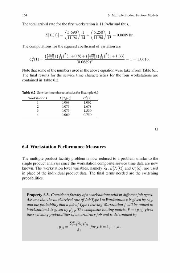
164 6 Multiple Product Factory Models
The total arrival rate for the first workstation is 11.94/hr and thus,
E[Ts(1)] =(
5.69011.94
)
114
+(
6.25011.94
)
115
= 0.0689 hr .
The computations for the squared coefficient of variation are
C2s (1) =
( 5.69011.94
)( 114
)2 (1 +0.8)+(6.250
11.94
)( 115
)2 (1 +1.33)(0.0689)2 − 1 = 1.0616 .
Note that some of the numbers used in the above equation were taken from Table 6.1.The final results for the service time characteristics for the four workstations arecontained in Table 6.2.
Table 6.2 Service time characteristics for Example 6.3
Workstation k E [Ts(k)] C2s (k)
1 0.069 1.0622 0.073 1.6783 0.075 1.5304 0.060 0.750
��
6.4 Workstation Performance Measures
The multiple product facility problem is now reduced to a problem similar to thesingle product analysis since the workstation composite service time data are nowknown. The workstation level variables, namely λk, E[Ts(k)] and C2
s (k), are usedin place of the individual product data. The final terms needed are the switchingprobabilities.
Property 6.3. Consider a factory of n workstations with m different job types.Assume that the total arrival rate of Job Type i to Workstation k is given by λi,k,and the probability that a job of Type i leaving Workstation j will be routed toWorkstation k is given by pi
j,k. The composite routing matrix, P = (p jk) givesthe switching probabilities of an arbitrary job and is determined by
p jk =∑m
i=1 λi j pijk
λ jfor j,k = 1, · · · ,n .

6.4 Workstation Performance Measures 165
Once the composite routing matrix is obtained, Property 5.8 can be used to de-termine the squared coefficients of variation for the workstation arrival streams, andthen the composite waiting times for an arbitrary job, CTq(k) for Workstation k, canbe derived using either Property 3.3 or 3.6. As long as there is no priority beinggiven to specific job types, all jobs experience the same queue; therefore, the meancycle time within Workstation k by Job Type i is given as
CTs(i,k) = CTq(k)+E[Ts(i,k)] . (6.5)
Combining Property 6.2 with Eq. (6.5) allows for the computation of the mean timethat each product type spends within the factory.
Property 6.4. Consider a factory of n workstations with m different job types.Assume that the external arrival rate of jobs of Type i to Workstation k isgiven by γi,k, and the total arrival rate of Job Type i to Workstation k is givenby λi,k. Furthermore assume that the mean time spent waiting for processingin Workstation k by an arbitrary job (namely, CTq(k)) has been determined.Then the mean time spent within the factory by a Type i job is given by
CT is =
∑nk=1 λik(CTq(k)+E[Ts(i,k)])
∑nj=1 γi j
for i = 1, · · · ,m.
Conditional cycle time information for individual products given their destination(such as good or bad parts) is considerably more complex and requires a Markovprocess modeling approach [4] beyond the scope of this book.
Example 6.4. We now complete the analysis of the factory contained in Exam-ples 6.1–6.3. The matrix of probabilities are obtained from Property 6.3. For ex-ample, the probability of going from Workstation 2 to Workstation 1 is determinedas
p21 =λ12 p1
21 +λ22 p221
λ2=
4.267(0.1)+6.667(0)10.934
= 0.039 .
Continuing with the other workstations should yield
P =
⎡
⎢
⎢
⎣
0 0.706 0.294 00.039 0 0.351 0.6100.024 0 0 0.5260.100 0.200 0.300 0
⎤
⎥
⎥
⎦
.
The analysis required to obtain the mean waiting times in the workstations is thesame procedure as for individual product systems once the composite product dataand transition probability matrix P have been developed. The squared coefficient of
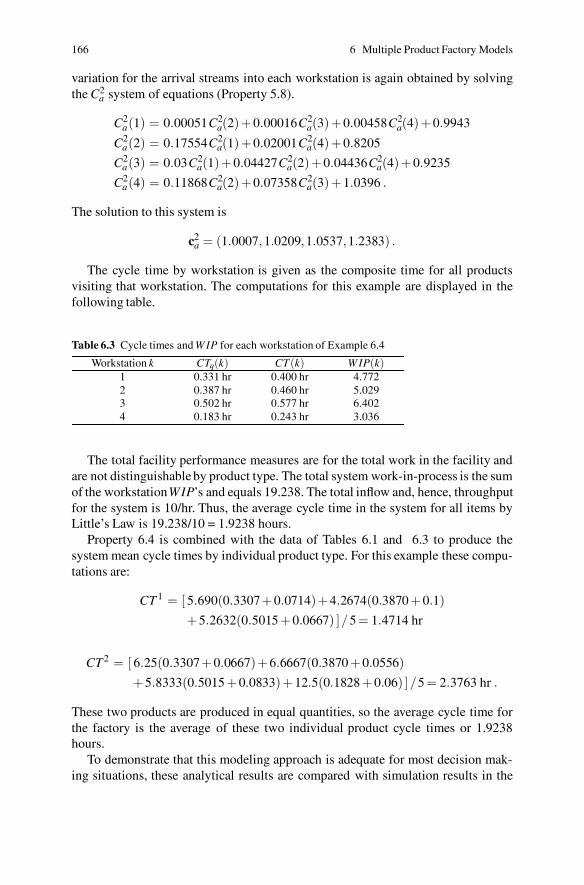
166 6 Multiple Product Factory Models
variation for the arrival streams into each workstation is again obtained by solvingthe C2
a system of equations (Property 5.8).
C2a(1) = 0.00051C2
a(2)+0.00016C2a(3)+0.00458C2
a(4)+0.9943
C2a(2) = 0.17554C2
a(1)+0.02001C2a(4)+0.8205
C2a(3) = 0.03C2
a(1)+0.04427C2a(2)+0.04436C2
a(4)+0.9235
C2a(4) = 0.11868C2
a(2)+0.07358C2a(3)+1.0396 .
The solution to this system is
c2a = (1.0007,1.0209,1.0537,1.2383) .
The cycle time by workstation is given as the composite time for all productsvisiting that workstation. The computations for this example are displayed in thefollowing table.
Table 6.3 Cycle times and W IP for each workstation of Example 6.4
Workstation k CTq(k) CT(k) W IP(k)1 0.331 hr 0.400 hr 4.7722 0.387 hr 0.460 hr 5.0293 0.502 hr 0.577 hr 6.4024 0.183 hr 0.243 hr 3.036
The total facility performance measures are for the total work in the facility andare not distinguishable by product type. The total system work-in-process is the sumof the workstationWIP’s and equals 19.238. The total inflow and, hence, throughputfor the system is 10/hr. Thus, the average cycle time in the system for all items byLittle’s Law is 19.238/10 = 1.9238 hours.
Property 6.4 is combined with the data of Tables 6.1 and 6.3 to produce thesystem mean cycle times by individual product type. For this example these compu-tations are:
CT 1 = [ 5.690(0.3307+0.0714)+4.2674(0.3870 +0.1)+5.2632(0.5015 +0.0667) ]/5 = 1.4714 hr
CT2 = [ 6.25(0.3307+0.0667)+6.6667(0.3870 +0.0556)+5.8333(0.5015 +0.0833)+12.5(0.1828 +0.06) ]/5 = 2.3763 hr .
These two products are produced in equal quantities, so the average cycle time forthe factory is the average of these two individual product cycle times or 1.9238hours.
To demonstrate that this modeling approach is adequate for most decision mak-ing situations, these analytical results are compared with simulation results in the

6.5 Processing Step Modeling Paradigm 167
following table. All of the critical parameters are close enough for the analyticalmodel to be a usable tool for decision purposes. Due to the quantity of the data, theinformation is given by rows for each workstation in Table 6.4. One row labeled Si for simulation results for Workstation i, and the associated analytical results in thefollowing row labeled A i.
Table 6.4 Comparison of simulation and analytical results for Example 6.4
Workstation CT W IP E [Ta] C2[Ta] E [Td] C2[Td ]S 1 0.398 4.744 0.084 1.001 0.084 1.050A 1 0.400 4.772 0.084 1.000 0.084 1.042S 2 0.427 4.677 0.091 1.028 0.091 1.443A 2 0.460 5.029 0.091 1.021 0.091 1.440S 3 0.569 6.309 0.090 1.035 0.090 1.397A 3 0.577 6.402 0.090 1.053 0.090 1.389S 4 0.248 3.107 0.080 1.330 0.080 1.044A 4 0.243 3.036 0.080 1.238 0.080 0.983
S sys 1.888 18.84 — — — —A sys 1.924 19.24 — — — —
��
• Suggestion: Do Problems 6.1–6.2 and 6.5–6.11.
6.5 Processing Step Modeling Paradigm
To this point, all analyses have considered that every visit to a workstation was prob-abilistically identical to all other visits to the same workstation. In other words, themean and standard deviation of processing time was the same whenever the sametype of job visited the same workstation. Furthermore, the switching probabilitiesonly depended on job type and not on whether or not the job was visiting the work-station for the first or the second time. There are many facilities where jobs makemore than one scheduled visit to various workstations and the processing character-istics are different for the various visits. These re-entrant flow systems are prevalentin the semiconductor industry as well as many job shop production type facilities.When a job requires a different processing time distribution from visit to visit orwhen a job is scheduled to visit a workstation more than once, it is necessary tokeep track of not only the job location but also the visit number to that location. Toaccomplish this extra requirement for job location control, a data description methodis used that is based on the process step that the job is undergoing.
The processing step modeling paradigm is a rather straight forward method ofaccomplishing the informational requirements of re-entrant flow systems. The ideais to list the processing steps that a job must go through during the production pro-cess. Associated with each processing step is the information needed for processingthat includes the workstation being visited and the processing time characteristics.
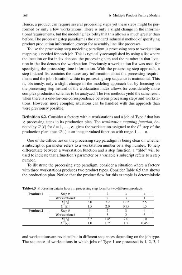
168 6 Multiple Product Factory Models
Hence, a product can require several processing steps yet these steps might be per-formed by only a few workstations. There is only a slight change in the informa-tional requirements, but the modeling flexibility that this allows is much greater thanbefore. The processing step paradigm is the standard industrial method of specifyingproduct production information, except for assembly line like processes.
To use the processing step modeling paradigm, a processing step to workstationmapping is needed for each job. This is typically accomplished by using a list wherethe location or list index denotes the processing step and the number in that loca-tion in the list denotes the workstation. Previously a workstation list was used forspecifying the processing time information. With the processing step approach, astep indexed list contains the necessary information about the processing require-ments and the job’s location within its processing step sequence is maintained. Thisis, obviously, only a slight change in the modeling approach but by focusing onthe processing step instead of the workstation index allows for considerably morecomplex production schemes to be analyzed. The two methods yield the same resultwhen there is a one-for-one correspondence between processing steps and worksta-tions. However, more complex situations can be handled with this approach thanwere previously possible.
Definition 6.2. Consider a factory with n workstations and a job of Type i that hasνi processing steps in its production plan. The workstation mapping function, de-noted by wi(�) for � = 1, · · · ,νi, gives the workstation assigned to the �th step of theproduction plan; thus wi(·) is an integer-valued function with range 1, · · · ,n.
One of the difficulties on the processing step paradigm is being clear on whethera subscript or parameter refers to a workstation number or a step number. To helpdifferentiate between a workstation function and a step function, a “tilde” will beused to indicate that a function’s parameter or a variable’s subscript refers to a stepnumber.
To illustrate the processing step paradigm, consider a situation where a factorywith three workstations produces two product types. Consider Table 6.5 that showsthe production plan. Notice that the product flow for this example is deterministic
Table 6.5 Processing data in hours in processing step form for two different products
Product 1 Step # 1 2 3 4Workstation # 1 2 3 1
E [Ts] 3.0 7.2 1.62 2.5C2[Ts] 1.5 2.0 0.75 1.5
Product 2 Step # 1 2 3 4Workstation # 1 3 2 3
E [Ts] 3.2 1.45 7.0 1.0C2[Ts] 1.0 1.75 1.7 0.45
and workstations are revisited but in different sequences depending on the job type.The sequence of workstations in which jobs of Type 1 are processed is 1, 2, 3, 1
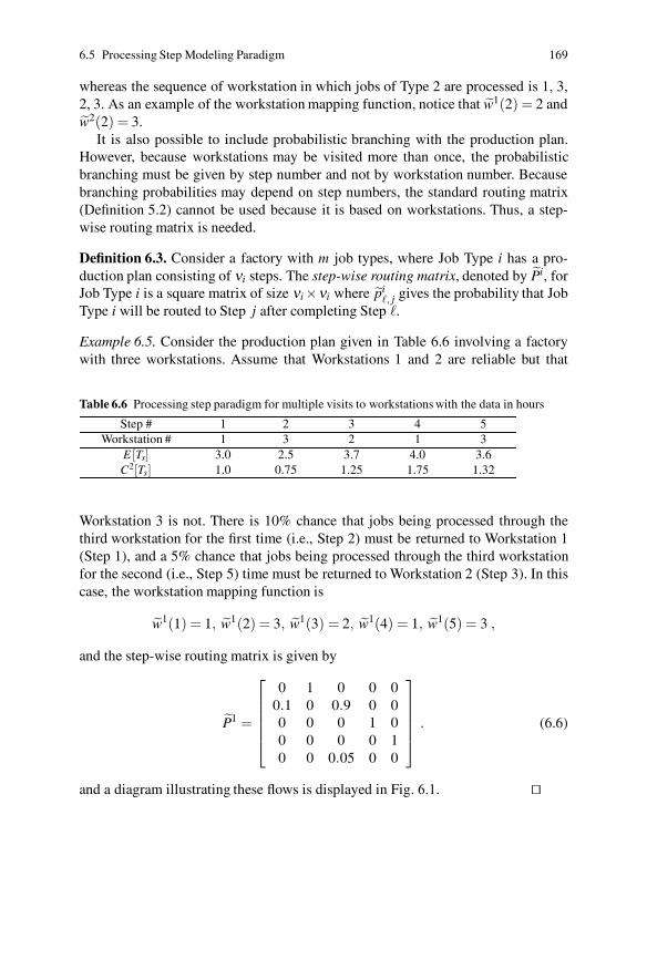
6.5 Processing Step Modeling Paradigm 169
whereas the sequence of workstation in which jobs of Type 2 are processed is 1, 3,2, 3. As an example of the workstation mapping function, notice that w1(2) = 2 andw2(2) = 3.
It is also possible to include probabilistic branching with the production plan.However, because workstations may be visited more than once, the probabilisticbranching must be given by step number and not by workstation number. Becausebranching probabilities may depend on step numbers, the standard routing matrix(Definition 5.2) cannot be used because it is based on workstations. Thus, a step-wise routing matrix is needed.
Definition 6.3. Consider a factory with m job types, where Job Type i has a pro-duction plan consisting of νi steps. The step-wise routing matrix, denoted by ˜Pi, forJob Type i is a square matrix of size νi×νi where pi
�, j gives the probability that JobType i will be routed to Step j after completing Step �.
Example 6.5. Consider the production plan given in Table 6.6 involving a factorywith three workstations. Assume that Workstations 1 and 2 are reliable but that
Table 6.6 Processing step paradigm for multiple visits to workstations with the data in hours
Step # 1 2 3 4 5Workstation # 1 3 2 1 3
E [Ts] 3.0 2.5 3.7 4.0 3.6C2[Ts] 1.0 0.75 1.25 1.75 1.32
Workstation 3 is not. There is 10% chance that jobs being processed through thethird workstation for the first time (i.e., Step 2) must be returned to Workstation 1(Step 1), and a 5% chance that jobs being processed through the third workstationfor the second (i.e., Step 5) time must be returned to Workstation 2 (Step 3). In thiscase, the workstation mapping function is
w1(1) = 1, w1(2) = 3, w1(3) = 2, w1(4) = 1, w1(5) = 3 ,
and the step-wise routing matrix is given by
˜P1 =
⎡
⎢
⎢
⎢
⎢
⎣
0 1 0 0 00.1 0 0.9 0 00 0 0 1 00 0 0 0 10 0 0.05 0 0
⎤
⎥
⎥
⎥
⎥
⎦
. (6.6)
and a diagram illustrating these flows is displayed in Fig. 6.1. ��
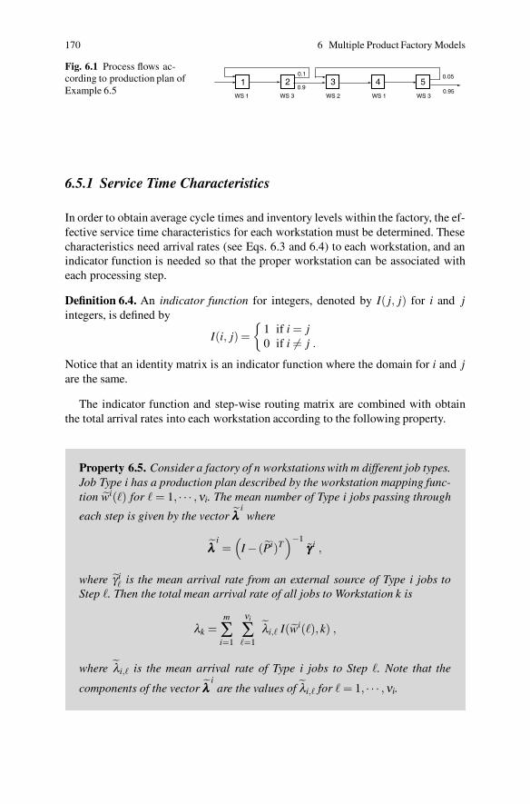
170 6 Multiple Product Factory Models
Fig. 6.1 Process flows ac-cording to production plan ofExample 6.5
1 2 3 4 50.9
0.1 0.05
0.95WS 1 WS 3 WS 3WS 1WS 2
6.5.1 Service Time Characteristics
In order to obtain average cycle times and inventory levels within the factory, the ef-fective service time characteristics for each workstation must be determined. Thesecharacteristics need arrival rates (see Eqs. 6.3 and 6.4) to each workstation, and anindicator function is needed so that the proper workstation can be associated witheach processing step.
Definition 6.4. An indicator function for integers, denoted by I( j, j) for i and jintegers, is defined by
I(i, j) ={
1 if i = j0 if i �= j .
Notice that an identity matrix is an indicator function where the domain for i and jare the same.
The indicator function and step-wise routing matrix are combined with obtainthe total arrival rates into each workstation according to the following property.
Property 6.5. Consider a factory of n workstations with m different job types.Job Type i has a production plan described by the workstation mapping func-tion wi(�) for � = 1, · · · ,νi. The mean number of Type i jobs passing through
each step is given by the vector ˜λλλi
where
˜λλλi=(
I − (˜Pi)T)−1
γγγ i ,
where ˜γ i� is the mean arrival rate from an external source of Type i jobs to
Step �. Then the total mean arrival rate of all jobs to Workstation k is
λk =m
∑i=1
νi
∑�=1
˜λi,� I(wi(�),k) ,
where ˜λi,� is the mean arrival rate of Type i jobs to Step �. Note that the
components of the vector ˜λλλi
are the values of ˜λi,� for � = 1, · · · ,νi.
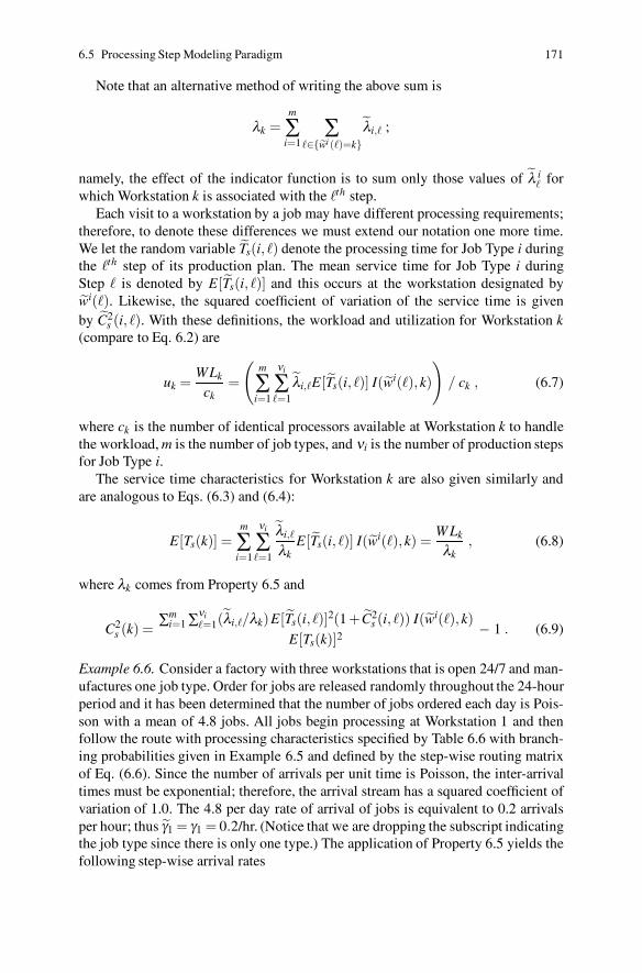
6.5 Processing Step Modeling Paradigm 171
Note that an alternative method of writing the above sum is
λk =m
∑i=1
∑�∈{wi (�)=k}
˜λi,� ;
namely, the effect of the indicator function is to sum only those values of ˜λ i� for
which Workstation k is associated with the �th step.Each visit to a workstation by a job may have different processing requirements;
therefore, to denote these differences we must extend our notation one more time.We let the random variable ˜Ts(i, �) denote the processing time for Job Type i duringthe �th step of its production plan. The mean service time for Job Type i duringStep � is denoted by E[˜Ts(i, �)] and this occurs at the workstation designated bywi(�). Likewise, the squared coefficient of variation of the service time is givenby ˜C2
s (i, �). With these definitions, the workload and utilization for Workstation k(compare to Eq. 6.2) are
uk =WLk
ck=
(
m
∑i=1
νi
∑�=1
˜λi,�E[˜Ts(i, �)] I(wi(�),k)
)
/ ck , (6.7)
where ck is the number of identical processors available at Workstation k to handlethe workload, m is the number of job types, and νi is the number of production stepsfor Job Type i.
The service time characteristics for Workstation k are also given similarly andare analogous to Eqs. (6.3) and (6.4):
E[Ts(k)] =m
∑i=1
νi
∑�=1
˜λi,�
λkE[˜Ts(i, �)] I(wi(�),k) =
W Lk
λk, (6.8)
where λk comes from Property 6.5 and
C2s (k) =
∑mi=1 ∑νi
�=1(˜λi,�/λk)E[˜Ts(i, �)]2(1 + ˜C2
s (i, �)) I(wi(�),k)E[Ts(k)]2
− 1 . (6.9)
Example 6.6. Consider a factory with three workstations that is open 24/7 and man-ufactures one job type. Order for jobs are released randomly throughout the 24-hourperiod and it has been determined that the number of jobs ordered each day is Pois-son with a mean of 4.8 jobs. All jobs begin processing at Workstation 1 and thenfollow the route with processing characteristics specified by Table 6.6 with branch-ing probabilities given in Example 6.5 and defined by the step-wise routing matrixof Eq. (6.6). Since the number of arrivals per unit time is Poisson, the inter-arrivaltimes must be exponential; therefore, the arrival stream has a squared coefficient ofvariation of 1.0. The 4.8 per day rate of arrival of jobs is equivalent to 0.2 arrivalsper hour; thus ˜γ1 = γ1 = 0.2/hr. (Notice that we are dropping the subscript indicatingthe job type since there is only one type.) The application of Property 6.5 yields thefollowing step-wise arrival rates
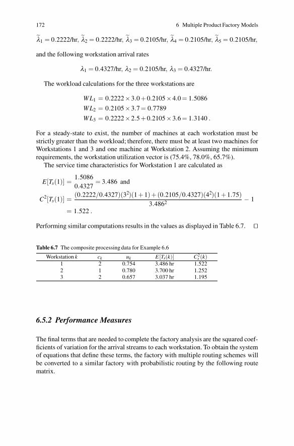
172 6 Multiple Product Factory Models
˜λ1 = 0.2222/hr, ˜λ2 = 0.2222/hr, ˜λ3 = 0.2105/hr, ˜λ4 = 0.2105/hr, ˜λ5 = 0.2105/hr,
and the following workstation arrival rates
λ1 = 0.4327/hr, λ2 = 0.2105/hr, λ3 = 0.4327/hr.
The workload calculations for the three workstations are
WL1 = 0.2222×3.0 +0.2105×4.0 = 1.5086
WL2 = 0.2105×3.7 = 0.7789
WL3 = 0.2222×2.5 +0.2105×3.6 = 1.3140 .
For a steady-state to exist, the number of machines at each workstation must bestrictly greater than the workload; therefore, there must be at least two machines forWorkstations 1 and 3 and one machine at Workstation 2. Assuming the minimumrequirements, the workstation utilization vector is (75.4%, 78.0%, 65.7%).
The service time characteristics for Workstation 1 are calculated as
E[Ts(1)] =1.50860.4327
= 3.486 and
C2[Ts(1)] =(0.2222/0.4327)(32)(1 +1)+(0.2105/0.4327)(42)(1 +1.75)
3.4862 − 1
= 1.522 .
Performing similar computations results in the values as displayed in Table 6.7. ��
Table 6.7 The composite processing data for Example 6.6
Workstation k ck uk E [Ts(k)] C2s (k)
1 2 0.754 3.486 hr 1.5222 1 0.780 3.700 hr 1.2523 2 0.657 3.037 hr 1.195
6.5.2 Performance Measures
The final terms that are needed to complete the factory analysis are the squared coef-ficients of variation for the arrival streams to each workstation. To obtain the systemof equations that define these terms, the factory with multiple routing schemes willbe converted to a similar factory with probabilistic routing by the following routematrix.

6.5 Processing Step Modeling Paradigm 173
Property 6.6. Consider a factory of n workstations with m different job types.Job Type i has a production plan described by the workstation mapping func-tion wi(�) for � = 1, · · · ,νi. The workstation routing matrix, P is defined, fork = 1, · · · ,n, by
pk, j =
(
m
∑i=1
νi
∑�=1
νi
∑r=1
˜λi,� pi�,r I(wi(�),k) I(wi(r), j)
)
/ λk ,
where the terms ˜λi,� and λk are determined by Property 6.5.
Our goal here is to determine the characteristics of the arrival streams to theworkstations, therefore, we need the coefficient of variation for the external arrivals.Let these be denoted by ˜C2
a(i,0, �); in other words, ˜C2a(i,0, �) is the squared coeffi-
cient of variation for the inter-arrival times of Job Type i from an external source thatenter the production process at Step � of the ith production plan. The characteristicsof the external arrival streams are given, for Workstation k, by
γk =m
∑i=1
νi
∑�=1
˜γ i� I(wi(�),k) , (6.10)
and
C2a(0, j) =
(
m
∑i=1
νi
∑�=1
˜γ i�˜C2
a(i,0, �) I(wi(�),k)
)
/ γk . (6.11)
The system of equations defined by Property 5.8 or 5.9 can now be used to find thesquared coefficients of variation for the arrival streams to each workstation.
Example 6.7. Example 6.6 can now be completed (Fig. 6.1). The associated averageproduct routing matrix for the three workstations obtained from Property 6.6 is
P =
⎡
⎣
0 0 11 0 00 0.538 0
⎤
⎦ .
The system of equations for computing the coefficients of variation for the averageproduct arrival streams at each workstation is
C2a(1) =
0.20.4327
(1)+0.21050.4327
[(
1−u22
)
C2a(2)+u2
2C2s (2)]
= 0.1905C2a(2)+0.8328
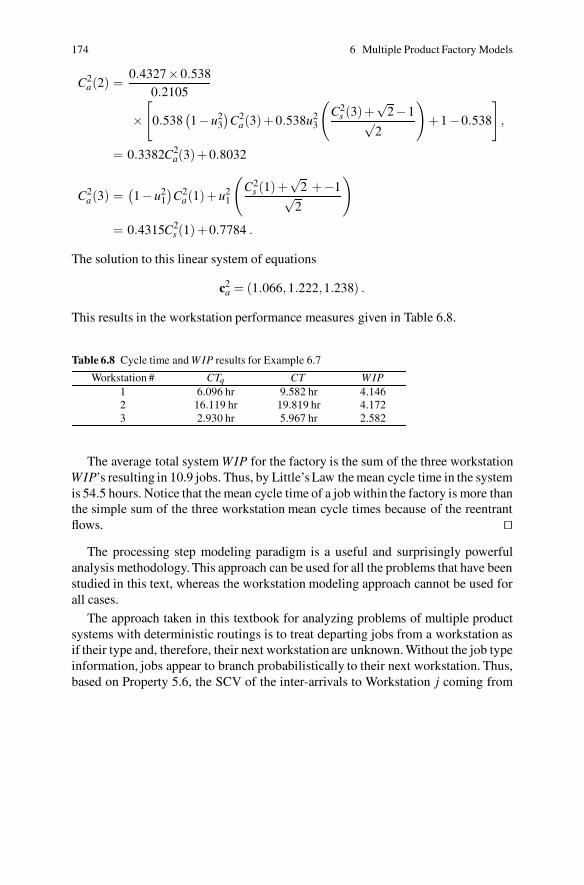
174 6 Multiple Product Factory Models
C2a(2) =
0.4327×0.5380.2105
×[
0.538(
1−u23
)
C2a(3)+0.538u2
3
(
C2s (3)+
√2−1√
2
)
+1−0.538
]
,
= 0.3382C2a(3)+0.8032
C2a(3) =
(
1−u21
)
C2a(1)+u2
1
(
C2s (1)+
√2 +−1√
2
)
= 0.4315C2s (1)+0.7784 .
The solution to this linear system of equations
c2a = (1.066,1.222,1.238) .
This results in the workstation performance measures given in Table 6.8.
Table 6.8 Cycle time and W IP results for Example 6.7
Workstation # CTq CT W IP1 6.096 hr 9.582 hr 4.1462 16.119 hr 19.819 hr 4.1723 2.930 hr 5.967 hr 2.582
The average total system WIP for the factory is the sum of the three workstationWIP’s resulting in 10.9 jobs. Thus, by Little’s Law the mean cycle time in the systemis 54.5 hours. Notice that the mean cycle time of a job within the factory is more thanthe simple sum of the three workstation mean cycle times because of the reentrantflows. ��
The processing step modeling paradigm is a useful and surprisingly powerfulanalysis methodology. This approach can be used for all the problems that have beenstudied in this text, whereas the workstation modeling approach cannot be used forall cases.
The approach taken in this textbook for analyzing problems of multiple productsystems with deterministic routings is to treat departing jobs from a workstation asif their type and, therefore, their next workstation are unknown. Without the job typeinformation, jobs appear to branch probabilistically to their next workstation. Thus,based on Property 5.6, the SCV of the inter-arrivals to Workstation j coming from

6.5 Processing Step Modeling Paradigm 175
Fig. 6.2 Illustration of a multiple product deterministic routing process with the products beingrepresented by distinct symbols
Workstation k, C2a(k, j) is obtained from the departing workstation’s composite C2
dby
C2a(k, j) = pk, jC
2d +1− pk, j , (6.12)
where pk, j is the job’s branching probability derived from Property 6.6. For prob-abilistic (Markovian) routings, this SCV adjustment is mathematically exact. Butfor deterministic routings, this approach can be significantly inaccurate, especiallywhen there are only a few deterministic routes with very little re-entrant flows. Thepurpose of this section is to present an alternate method for determining the squaredcoefficient of variation for the workstation arrival streams, although for most sit-uations, the models presented above should prove to be sufficiently accurate formost purposes. The following example demonstrates the potential for inaccurateestimates.
Example 6.8. To illustrate the potential inaccuracy of (6.12), consider a workstationthat processes three products with each going to a specified and different worksta-tion upon leaving this workstation as illustrated by Fig. 6.2. For purposes of thisexample, the workstation of the figure will be designated as Workstation 4, and theProducts 1, 2, and 3 are sent to Workstations 1, 2, and 3, respectively. The indi-vidual arrival stream information (into this workstation) and necessary workstationprocessing time parameters are listed in the following table.
Table 6.9 Arrival stream and service time characteristics by product type for Fig. 6.2
Product i λi C2a(i) E [Si] C2
s (i)1 1 1.50 0.3 1.52 1 2.50 0.3 1.53 1 0.75 0.3 1.5
The workstation utilization factor is 3(0.3) = 0.9; there is only one machine avail-able. The C2
d for the composite departure stream, using the typical i.i.d. approxima-tion of Property 5.2 is
C2d(4) = (1−u2
4)Ca(4)2 +u24C2
s (4) (6.13)
=(
1−0.92) (1.50 +2.50 +0.75)3
+0.92(1.5) = 1.516 .
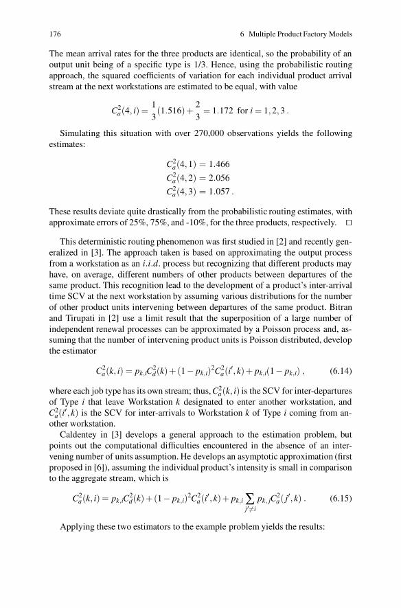
176 6 Multiple Product Factory Models
The mean arrival rates for the three products are identical, so the probability of anoutput unit being of a specific type is 1/3. Hence, using the probabilistic routingapproach, the squared coefficients of variation for each individual product arrivalstream at the next workstations are estimated to be equal, with value
C2a(4, i) =
13(1.516)+
23
= 1.172 for i = 1,2,3 .
Simulating this situation with over 270,000 observations yields the followingestimates:
C2a(4,1) = 1.466
C2a(4,2) = 2.056
C2a(4,3) = 1.057 .
These results deviate quite drastically from the probabilistic routing estimates, withapproximate errors of 25%, 75%, and -10%, for the three products, respectively. ��
This deterministic routing phenomenon was first studied in [2] and recently gen-eralized in [3]. The approach taken is based on approximating the output processfrom a workstation as an i.i.d. process but recognizing that different products mayhave, on average, different numbers of other products between departures of thesame product. This recognition lead to the development of a product’s inter-arrivaltime SCV at the next workstation by assuming various distributions for the numberof other product units intervening between departures of the same product. Bitranand Tirupati in [2] use a limit result that the superposition of a large number ofindependent renewal processes can be approximated by a Poisson process and, as-suming that the number of intervening product units is Poisson distributed, developthe estimator
C2a(k, i) = pk,iC
2d(k)+(1− pk,i)2C2
a(i′,k)+ pk,i(1− pk,i) , (6.14)
where each job type has its own stream; thus, C2a(k, i) is the SCV for inter-departures
of Type i that leave Workstation k designated to enter another workstation, andC2
a(i′,k) is the SCV for inter-arrivals to Workstation k of Type i coming from an-other workstation.
Caldentey in [3] develops a general approach to the estimation problem, butpoints out the computational difficulties encountered in the absence of an inter-vening number of units assumption. He develops an asymptotic approximation (firstproposed in [6]), assuming the individual product’s intensity is small in comparisonto the aggregate stream, which is
C2a(k, i) = pk,iC
2d(k)+(1− pk,i)2C2
a(i′,k)+ pk,i ∑
j′�=i
pk, jC2a( j′,k) . (6.15)
Applying these two estimators to the example problem yields the results:

6.6 Group Technology and Cellular Manufacturing 177
Table 6.10 Comparisons of three methods for estimating splitting with simulation results
Method C2a(4,1) C2
a(4,2) C2a(4,3)
Simulation 1.466 2.056 1.057Markovian Routing 1.172 1.172 1.172Poisson (Eq. 6.14) 1.394 1.839 1.061
Asymptotic (Eq. 6.15) 1.533 1.866 1.283
For this situation, the Poisson approximation for the number of intervening unitsyields the best overall approximation. However, other assumptions such as the as-sumption in [2] of a small number of intervening units approximations based on anErlang assumption might yield better approximations. The Erlang approach unfor-tunately does not result in an analytical expression and numerical evaluations mustbe made.
• Suggestion: Do Problems 6.3–6.4, 6.12 and 6.14.
6.6 Group Technology and Cellular Manufacturing
Batch manufacturing is the most common form of production used in the UnitedStates [5, p. 420] making up approximately 50% of the production activity. Onemethod that attempts to make batch manufacturing more efficient is group tech-nology. The basic idea of group technology is to essentially establish sub-factorieswithin a factory with each sub-factory being dedicated to the production of a subsetof the total number of part types produced by the factory, where the part types havebeen grouped by common characteristics. (Of course, this concept can be appliedto the production of subsequences as well as the full production process for a parttype.) Thus, the machines of the factory are grouped into cells of machines neededto produce the job type family assigned to that sub-factory. Part families are chosenso that the parts have as similar processing operations as possible. The forming ofthese part families is called group technology.
Definition 6.5. Group technology is the analysis of processing operations with thegoal of determining the similarity of the processing functions and, hence, the group-ing of the associated parts for production purposes.
The normal factory organization is to group similar machines together and pro-duce all part types by routing each part through this one grouping of machines for agiven processing operation. However, group technology takes advantage of group-ing machines according to the similarities of the parts being manufactured which iscalled cellular manufacturing.
Definition 6.6. The concept of organizing the factory into sub-factories with thecapability to produce a technology group is called cellular manufacturing.
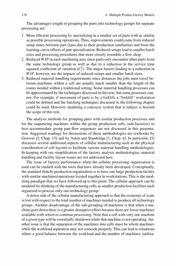
178 6 Multiple Product Factory Models
The advantages sought in grouping the parts into technology groups for separateprocessing are:
1. More efficient processing by specializing in a smaller set of parts with as similaras possible processing operations. Thus, improvements could come from reducedsetup times between part types due to their production similarities and from thelearning-curve effects of part specialization. Reduced setups lead to smaller batchsizes and processing procedures that more closely resemble a flow shop.
2. Reduced W IP in each machining area since parts only encounter other parts fromthe same technology group as well as due to a reduction in the service timesquared coefficient of variation (C2
s ). The major factors leading to a reduction inW IP, however, are the impacts of reduced setups and smaller batch sizes.
3. Reduced material handling requirements since distances the jobs must travel be-tween machines within a cell are usually much smaller than the length of theroutes needed within a traditional setting. Some material handling processes canbe approximated by the techniques discussed in this text, but some processes can-not. For example, if movement of parts is by a forklift, a “forklift” workstationcould be defined and the batching techniques discussed in the following chaptercould be used. However, modeling a conveyor system that is subject is beyondthe scope of this text.
The analysis methods for grouping parts with similar production processes andfor the sequencing machines within the group production cells (sub-factories) tobest accommodate group part-flow sequences are not discussed in this presenta-tion. Suggested readings for discussions of these methodologies are textbooks byGroover [5, Chap. 15] and by Askin and Standridge [1, Chap. 6]. In particular, [5]discusses several additional aspects of cellular manufacturing such as the physicalconsideration of cell layouts to facilitate various material handling methodologies.In keeping with our simplification of the factory analysis methodologies, materialhandling and facility layout issues are not addressed here.
The issue of factory performance when the cellular processing organization isused can be studied with the tools that have already been developed. Conceptually,the standard (batch) production organization is to have one large production facilitywith similar machines/operations located together in workstations. This is the mod-eling paradigm that we have followed up to this point. The cellular approach can bemodeled by thinking of the manufacturing cells as smaller production facilities eachorganized to process only one technology group.
A down side of the cellular manufacturing approach is that the economy of scaleis lost with respect to the total number of machines needed to produce all technologygroups. Another disadvantage of the sub-grouping of machines is that when a ma-chine goes down there is a greater disruptive effect because there are fewer machinesavailable with which to continue processing. Note that a cell with only one machineof a given type will be essentially shutdown while that machine is not operating. An-other issue is that the separation of the machines into cells must be whole machineswhile the workload separation may not coincide properly. This can lead to situationswhere a good balance between the workload and the number of machines (utiliza-
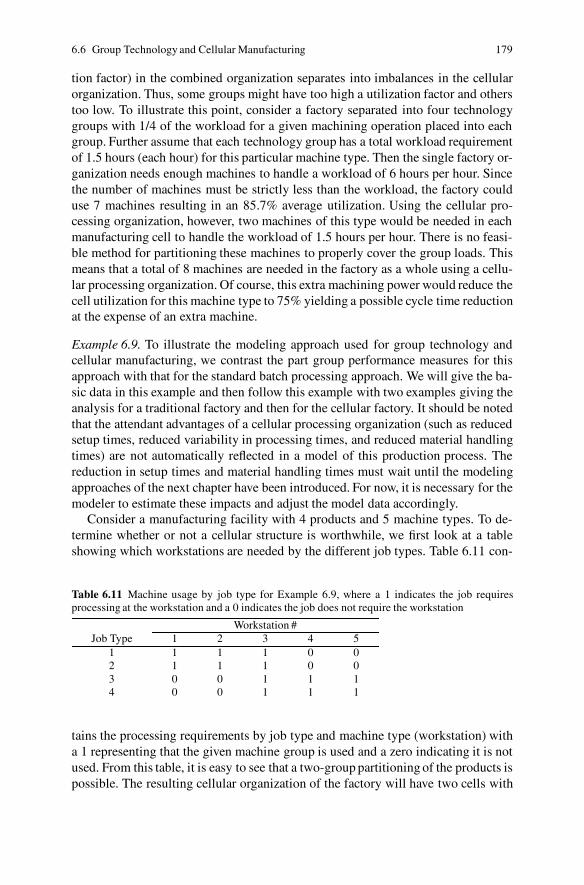
6.6 Group Technology and Cellular Manufacturing 179
tion factor) in the combined organization separates into imbalances in the cellularorganization. Thus, some groups might have too high a utilization factor and otherstoo low. To illustrate this point, consider a factory separated into four technologygroups with 1/4 of the workload for a given machining operation placed into eachgroup. Further assume that each technology group has a total workload requirementof 1.5 hours (each hour) for this particular machine type. Then the single factory or-ganization needs enough machines to handle a workload of 6 hours per hour. Sincethe number of machines must be strictly less than the workload, the factory coulduse 7 machines resulting in an 85.7% average utilization. Using the cellular pro-cessing organization, however, two machines of this type would be needed in eachmanufacturing cell to handle the workload of 1.5 hours per hour. There is no feasi-ble method for partitioning these machines to properly cover the group loads. Thismeans that a total of 8 machines are needed in the factory as a whole using a cellu-lar processing organization. Of course, this extra machining power would reduce thecell utilization for this machine type to 75% yielding a possible cycle time reductionat the expense of an extra machine.
Example 6.9. To illustrate the modeling approach used for group technology andcellular manufacturing, we contrast the part group performance measures for thisapproach with that for the standard batch processing approach. We will give the ba-sic data in this example and then follow this example with two examples giving theanalysis for a traditional factory and then for the cellular factory. It should be notedthat the attendant advantages of a cellular processing organization (such as reducedsetup times, reduced variability in processing times, and reduced material handlingtimes) are not automatically reflected in a model of this production process. Thereduction in setup times and material handling times must wait until the modelingapproaches of the next chapter have been introduced. For now, it is necessary for themodeler to estimate these impacts and adjust the model data accordingly.
Consider a manufacturing facility with 4 products and 5 machine types. To de-termine whether or not a cellular structure is worthwhile, we first look at a tableshowing which workstations are needed by the different job types. Table 6.11 con-
Table 6.11 Machine usage by job type for Example 6.9, where a 1 indicates the job requiresprocessing at the workstation and a 0 indicates the job does not require the workstation
Workstation #Job Type 1 2 3 4 5
1 1 1 1 0 02 1 1 1 0 03 0 0 1 1 14 0 0 1 1 1
tains the processing requirements by job type and machine type (workstation) witha 1 representing that the given machine group is used and a zero indicating it is notused. From this table, it is easy to see that a two-group partitioning of the products ispossible. The resulting cellular organization of the factory will have two cells with

180 6 Multiple Product Factory Models
both cells needing Workstation 3. So these three machines will need to be partitioned(if possible) into the cells according to the work demand in each group.
Each job type requires 4 processing steps as shown in Table 6.12. This table con-tains the mean arrival rate for each job type, the sequence in which the workstationsmust be visited, and the mean processing time at each step.
Table 6.12 Arrival rates, processing sequence, and mean service times by job type and processingstep for Example 6.9
Workstation Sequence Mean Service Timeby Step # by Step #
Job Type Arrival Rate 1 2 3 4 1 2 3 41 0.064/hr 3 1 2 1 8 hr 6 hr 4.5 hr 6 hr2 0.096/hr 1 2 3 1 5 hr 6 hr 8 hr 4 hr3 0.080/hr 4 3 5 4 2 hr 4 hr 8 hr 4 hr4 0.100/hr 3 4 5 3 7 hr 3 hr 2 hr 4 hr
The arrival processes are each assumed to be exponentially distributed (C2a = 1)
and the processing times are assumed to follow an Erlang-2 distribution (C2s = 1/2).
The number of machines at each workstation are 2, 1, 3, 1, and 1 for Workstations 1through 5, respectively. ��
Example 6.10. Traditional Factory Model. In this example, we summarize theanalysis of Sect. 6.5 for the data of Example 6.9. The standard (batch) process-ing organization model of this system has 5 workstations for processing the 4 parttypes.
The workload for each workstation (machine group) is computed by consideringall products that visit the workstation and the number of times they visit. For ex-ample, Workstation 1 is visited twice by Job Type 1 (6 hours processing on visit 1and 6 hours processing on visit 2) twice by Job Type 2 (5 hours processing on visit1 and 4 hours processing on visit 2). The release rate is 0.064 jobs/hour for Type 1and 0.096 jobs/hour for Type 2. Hence the total amount of work that is released forWorkstation 1 is
workload1 = (6 +6)0.064 +(5 +4)0.096 = 1.632 .
Thus, at least two machines are needed in Workstation 1. The utilization factor forWorkstation 1, u1, is the workload divided by the number of machines available(assuming 100% availability)
u1 = 1.632/2 = 0.816 .
A similar analysis for the other four workstations yields the results of Table 6.13.The expected processing time for Workstation 1 is a function of the three distinct
processing times (Job Type 1 uses the machine twice but has the same processingtime for each visit) and the relative frequencies of these visits. That is, the ma-chine processing time distribution characteristics are developed using the mixture

6.6 Group Technology and Cellular Manufacturing 181
Table 6.13 Workload and utilization factors for Example 6.10
Workstation # Num Machines Workload Utilization1 2 1.632 0.8162 1 0.864 0.8643 3 2.700 0.9004 1 0.780 0.7805 1 0.840 0.840
of distributions methodology (as in 1.6.3). That is, each visit to the machine by ajob can possibly have a different processing time distribution. Thus, we need to useEqs. (6.3) and (6.4) for the mean and SCV computations, respectively. For Work-station 1, the total arrival rate of jobs is 0.32 per hour (two inflows of Job Type 1 ata rate of 0.064 per hour and two inflows of Job Type 2 at a rate of 0.096 per hour).Thus, the mean processing time is computed as
E[S1] =(
0.0640.32
)
6 +(
0.0640.32
)
6 +(
0.0960.32
)
5 +(
0.0960.32
)
4 = 5.100 hr .
Recall that all processing times are assumed to be distributed according to an Erlang-2 with specified means. Thus, the SCV is computed as
E[S21] = 2
(
0.0640.32
)
62(1 +1/2)+(
0.0960.32
)
52(1 +1/2)
+(
0.0960.32
)
42(1 +1/2) = 40.05 hr2
C2s (1) =
E[S21]−E[S1]2
E[S1]2=
40.05−26.0126.01
= 0.540 .
Continuing with the other four workstations yields the data of Table 6.14.
Table 6.14 Service time characteristics for Example 6.10
Workstation k λk E [Sk] C2s (k)
1 0.32/hr 5.100 hr 0.5402 0.16/hr 5.400 hr 0.5283 0.44/hr 6.136 hr 0.6314 0.26/hr 3.000 hr 0.6035 0.18/hr 4.667 hr 1.112
The final step before obtained the system of equations defining the squared co-efficients of variation is the calculation of the probabilities of a job leaving oneworkstation being sent to another workstation; namely, implementing Property 6.6which yields
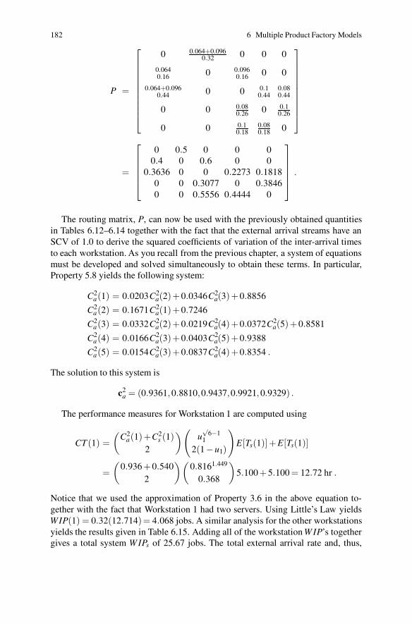
182 6 Multiple Product Factory Models
P =
⎡
⎢
⎢
⎢
⎢
⎢
⎢
⎢
⎢
⎢
⎣
0 0.064+0.0960.32 0 0 0
0.0640.16 0 0.096
0.16 0 0
0.064+0.0960.44 0 0 0.1
0.440.080.44
0 0 0.080.26 0 0.1
0.26
0 0 0.10.18
0.080.18 0
⎤
⎥
⎥
⎥
⎥
⎥
⎥
⎥
⎥
⎥
⎦
=
⎡
⎢
⎢
⎢
⎢
⎣
0 0.5 0 0 00.4 0 0.6 0 0
0.3636 0 0 0.2273 0.18180 0 0.3077 0 0.38460 0 0.5556 0.4444 0
⎤
⎥
⎥
⎥
⎥
⎦
.
The routing matrix, P, can now be used with the previously obtained quantitiesin Tables 6.12–6.14 together with the fact that the external arrival streams have anSCV of 1.0 to derive the squared coefficients of variation of the inter-arrival timesto each workstation. As you recall from the previous chapter, a system of equationsmust be developed and solved simultaneously to obtain these terms. In particular,Property 5.8 yields the following system:
C2a(1) = 0.0203C2
a(2)+0.0346C2a(3)+0.8856
C2a(2) = 0.1671C2
a(1)+0.7246
C2a(3) = 0.0332C2
a(2)+0.0219C2a(4)+0.0372C2
a(5)+0.8581
C2a(4) = 0.0166C2
a(3)+0.0403C2a(5)+0.9388
C2a(5) = 0.0154C2
a(3)+0.0837C2a(4)+0.8354 .
The solution to this system is
c2a = (0.9361,0.8810,0.9437,0.9921,0.9329) .
The performance measures for Workstation 1 are computed using
CT (1) =(
C2a(1)+C2
s (1)2
)
(
u√
6−11
2(1−u1)
)
E[Ts(1)]+E[Ts(1)]
=(
0.936 +0.5402
)(
0.8161.449
0.368
)
5.100 +5.100 = 12.72 hr .
Notice that we used the approximation of Property 3.6 in the above equation to-gether with the fact that Workstation 1 had two servers. Using Little’s Law yieldsWIP(1) = 0.32(12.714)= 4.068 jobs. A similar analysis for the other workstationsyields the results given in Table 6.15. Adding all of the workstation W IP’s togethergives a total system W IPs of 25.67 jobs. The total external arrival rate and, thus,
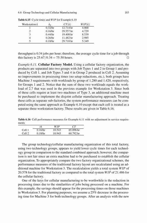
6.6 Group Technology and Cellular Manufacturing 183
Table 6.15 Cycle times and W IP for Example 6.10
Workstation k λk CT(k) W IP(k)1 0.32/hr 12.714 hr 4.0682 0.16/hr 29.557 hr 4.7293 0.44/hr 19.408 hr 8.5394 0.26/hr 11.482 hr 2.9855 0.18/hr 29.718 hr 5.349
throughput is 0.34 jobs per hour; therefore, the average cycle time for a job throughthis factory is 25.67/0.34 = 75.50 hours. ��
Example 6.11. Cellular Factory Model. Using a cellular factory organization, theproducts are separated into two groups with Job Types 1 and 2 in Group 1 and pro-duced by Cell 1, and Job Types 3 and 4 in Group 2 produced in Cell 2. Assumingno improvements in processing times (no setup reductions, etc.), both groups haveMachine 3 requirements with workloads by group of 1.280 and 1.420, respectively,for Groups 1 and 2. Notice that the sum of these two workloads equals the work-load of 2.7 that was used in the previous example for Workstation 3. Since bothof these cells require at least two machines of Type 3, an additional machine mustbe purchased to implement the disjoint cellular manufacturing approach. Treatingthese cells as separate sub-factories, the system performance measures can be com-puted using the same approach as Example 6.10 except that each cell is treated as aseparate three-workstation factory. These results are given in Table 6.16.
Table 6.16 Cell performance measures for Example 6.11 with no adjustment in service require-ments
th W IP CTCell 1 0.16/hr 10.543 65.896 hrCell 2 0.18/hr 10.943 60.792 hr
The group technology/cellular manufacturing organization of this total factory,using two technology groups, appears to yield lower cycle times for each technol-ogy group in comparison to the standard combined approach; however, the compar-ison is not fair since an extra machine had to be purchased to establish the cellularorganization. To appropriately compare the two factory organizational schemes, theperformance measures of the traditional factory layout are recalculated using an ad-ditional machine for Workstation 3. The recalculation yields a total system WIP of20.578 for the traditional factory as compared to the total system WIP of 21.486 forthe cellular factory.
One of the keys for cellular manufacturing to be worthwhile is the reduction inprocessing times due to the similarities of jobs being processed on a machine. Forthis example, the savings should appear for the processing times on those machinesin Workstation 3. For planning purposes, we assume a 25% decrease in the process-ing time for Machine 3 for both technology groups. After an analysis with the new
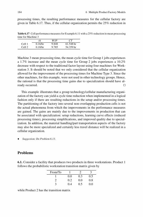
184 6 Multiple Product Factory Models
processing times, the resulting performance measures for the cellular factory aregiven in Table 6.17. Thus, if the cellular organization permits the 25% reduction in
Table 6.17 Cell performancemeasures for Example 6.11 with a 25% reduction in mean processingtime for Machine 3
th W IP CTCell 1 0.16/hr 9.848 61.548 hrCell 2 0.18/hr 9.785 54.359 hr
Machine 3 mean processing time, the mean cycle time for Group 1 jobs experiencesa 1.7% increase and the mean cycle time for Group 2 jobs experiences a 10.2%decrease with respect to the traditional factor layout using four machines for Work-station 3. It should be noted that we only considered that the cellular organizationallowed for the improvement of the processing times for Machine Type 3. Since theother machines, for this example, were not used in other technology groups. Hence,the rational is that the processing time gains due to specialization should have al-ready occurred. ��
This example illustrates that a group technology/cellular manufacturing organi-zation of the factory can yield a cycle time reduction when implemented in a logicalfashion only if there are resulting reductions in the setup and/or processing times.The partitioning of the factory into several non-overlapping production cells is notthe actual phenomena from which the improvements in the performance measuresare gained. The gains are mainly due to the improvements in production that canbe associated with specialization: setup reductions, learning curve effects (reducedprocessing times), processing simplifications, and improved quality due to special-ization. In addition, the material handling/part transportation aspects of the factorymay also be more specialized and certainly less travel distance will be realized in acellular organization.
• Suggestion: Do Problem 6.13.
Problems
6.1. Consider a facility that produces two products in three workstations. Product 1follows the probabilistic workstation transition matrix given by
From/To 1 2 31 0.0 0.3 0.52 0.2 0.0 0.83 0.4 0.5 0.0
while Product 2 has the transition matrix

Problems 185
From/To 1 2 31 0.0 0.6 0.42 0.3 0.0 0.73 0.4 0.1 0.0
The workstation processing time distributions are different by product. For Prod-uct 1, these data are
Workstation # E[Ts] C2s
1 1.1 hr 1.02 1.0 hr 1.53 0.6 hr 2.0
For Product 2, these data are
Workstation # E[Ts] C2s
1 0.25 hr 1.02 0.35 hr 1.53 0.60 hr 2.0
The mean release rate for Product 1 is 0.2 jobs per hour and for Product 2 is 0.3 jobsper hour, both Poisson distributed releases into Workstation 1.(a) Determine the minimum number of (identical) machines that must be placed ineach workstation so that a steady-state system results.(b) Using the number of machines determined in Part (a), find the workstation andsystem performance measures: cycle time, work-in-process, and throughput.
6.2. Resolve Problem 1 with machine availabilities less than one. Two sets of ma-chine availabilities and repair time data for the three workstations are given below.Compare these answers with those of Problem 1.(a)
Workstation # 1 2 3Availability 0.9 0.9 0.9
E[R] 1 hr 1 hr 1 hrC2[R] 1.5 1.75 2.0
(b)
Workstation # 1 2 3Availability 0.95 0.90 0.87
E[R] 42 min 60 min 72 minC2[R] 1.5 1.75 2.0
6.3. Consider a factory with the process flow as given in the following table.
Step # 1 2 3 4 5 6WS # 1 2 3 1 2 4E[Ts] 10 min 7.5 min 7.5 min 8.6 min 10 min 10.9 minV [Ts] 79.2 min2 68.4 min2 82.8 min2 72 min2 126 min2 90 min2

186 6 Multiple Product Factory Models
In addition, an inspection is preformed after the third processing step, and 10%of the jobs must be totally reworked and are returned to the beginning of process.Compute the system and workstation measures of effectiveness of throughput,W IPand cycle time. There are two machines in Workstations 1 and 2 and one machine inWorkstations 3 and 4. Consider an arrival rate of jobs of 5 per hour (exponentiallydistributed time between arrivals) from an external source.
6.4. Resolve Problem 6.3 with machine availabilities and repair time data given by:
Workstation # 1 2 3 4Availability 0.9 0.85 0.8 0.99
E[R] 1 hr 1 hr 1 hr 1 hrC2[R] 1 1 1 1
6.5. The Southwestern Specialties Company has a line of four products that theyproduce in their factory located in Houston, Texas. The Houston factory consists ofthree workstations (called Workstations 1, 2 and 3). The four products take differ-ent routes through the three workstations and have different numbers of processingsteps. There are currently three machines in Workstation 1 and 3, and one machinein Workstation 2.
Orders are released to the factory in a random fashion with the mean rate of totalorder releases being 7.68 per day. The random order release implies that the timebetween orders is exponentially distributed. The release of orders to the factor israndom with 20% of the orders being for Product 1, 30% for Product 2, 25% forProduct 3, and 25% for Product 4.
The processing step sequence and mean processing times in hours, are givenin the following table where the individual processing times follow an Erlang-2distribution.
Step # 1 2 3 4 5Product 1 Workstation # 3 1 2 1 —
Mean Time 8.0 6.0 1.7 6.0 —Product 2 Workstation # 1 2 3 2 1
Mean Time 5.0 1.6 8.0 1.5 5.0Product 3 Workstation # 2 1 2 3 1
Mean Time 1.9 4.0 2.2 8.0 4.0Product 4 Workstation # 3 1 2 — —
Mean Time 8.0 3.0 2.2 — —
What is the average cycle time for all products combined? What is the mean cycletime for each product?
6.6. This problem is designed to encompasses all of the basic components of build-ing a multiple product model. To help reduce the time to solve the problem, manyof the numerical values are given so that the entire problem need not be workedout. There are ten parts to the problem with several tables of numerical values beinggiven; however, many of the tables will contain incomplete information, so thoseplaces in the table should be filled in.

Problems 187
Fig. 6.3a Process routing forProduct 1 for Problem 6.6
Fig. 6.3b Process routing forProduct 2 for Problem 6.6
A company is developing a factory to produce two different products. Both prod-ucts use three distinct machining processes; thus, the factory will require three work-stations. Company management would like to know several things about the factorybefore it is built. To support this analysis engineering has developed estimates forthe necessary product processing information. This information is listed below, andFigs. 6.3a and 6.3b depict the product processing routings. Answer the questionsand fill in the missing data.
Mean processing times by product and workstation.
Product/WS 1 1 31 0.120 hr 0.100 hr 0.060 hr2 0.100 hr 0.035 hr 0.060 hr
SCV of the processing times by product and workstation.
Product/WS 1 1 31 0.7 0.8 0.92 0.8 0.9 1.0
Machine availabilities and repair time characteristics.
Workstation # 1 2 3Availability 0.90 0.95 0.93
E[R] 1.00 hr 1.00 hr 1.00 hrC2[R] 1.50 1.75 2.00
Answer the following questions and fill in the missing information.(a) Write the system of equations needed to find the mean flow rates into each work-station for Product 1. These equations would yield the following mean arrival ratesfor the two products into the three workstations:
Product/WS 1 2 31 9.5135/hr 6.7568/hr 9.4865/hr2 3.4326/hr 4.0439/hr 4.3260/hr
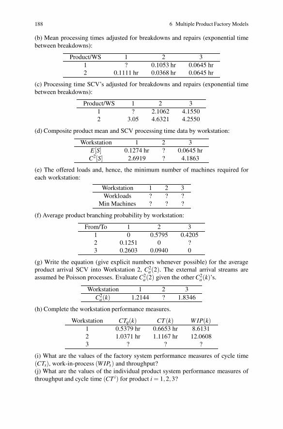
188 6 Multiple Product Factory Models
(b) Mean processing times adjusted for breakdowns and repairs (exponential timebetween breakdowns):
Product/WS 1 2 31 ? 0.1053 hr 0.0645 hr2 0.1111 hr 0.0368 hr 0.0645 hr
(c) Processing time SCV’s adjusted for breakdowns and repairs (exponential timebetween breakdowns):
Product/WS 1 2 31 ? 2.1062 4.15502 3.05 4.6321 4.2550
(d) Composite product mean and SCV processing time data by workstation:
Workstation 1 2 3E[S] 0.1274 hr ? 0.0645 hrC2[S] 2.6919 ? 4.1863
(e) The offered loads and, hence, the minimum number of machines required foreach workstation:
Workstation 1 2 3Workloads ? ? ?
Min Machines ? ? ?
(f) Average product branching probability by workstation:
From/To 1 2 31 0 0.5795 0.42052 0.1251 0 ?3 0.2603 0.0940 0
(g) Write the equation (give explicit numbers whenever possible) for the averageproduct arrival SCV into Workstation 2, C2
a(2). The external arrival streams areassumed be Poisson processes. Evaluate C2
a(2) given the other C2a(k)’s.
Workstation 1 2 3C2
a(k) 1.2144 ? 1.8346
(h) Complete the workstation performance measures.
Workstation CTq(k) CT (k) W IP(k)1 0.5379 hr 0.6653 hr 8.61312 1.0371 hr 1.1167 hr 12.06083 ? ? ?
(i) What are the values of the factory system performance measures of cycle time(CTs), work-in-process (WIPs) and throughput?(j) What are the values of the individual product system performance measures ofthroughput and cycle time (CT i) for product i = 1,2,3?
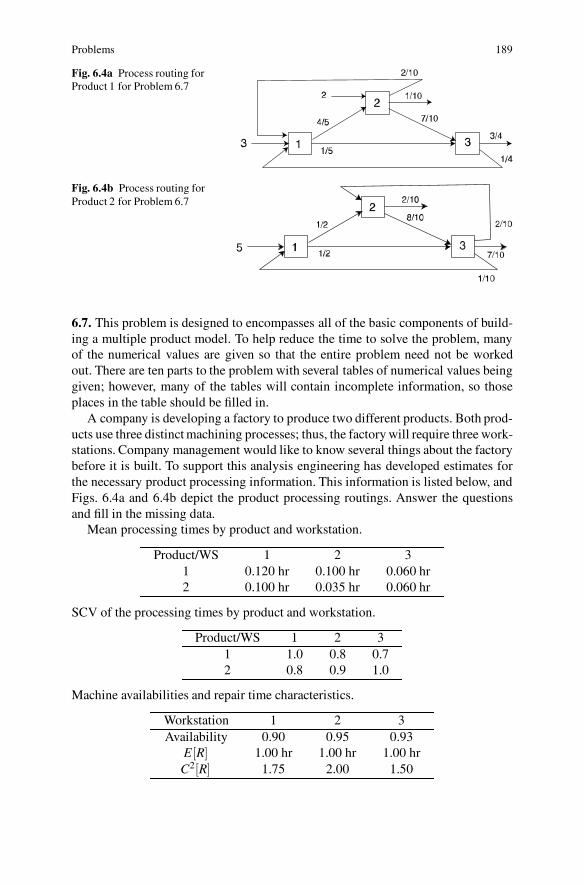
Problems 189
Fig. 6.4a Process routing forProduct 1 for Problem 6.7
Fig. 6.4b Process routing forProduct 2 for Problem 6.7
6.7. This problem is designed to encompasses all of the basic components of build-ing a multiple product model. To help reduce the time to solve the problem, manyof the numerical values are given so that the entire problem need not be workedout. There are ten parts to the problem with several tables of numerical values beinggiven; however, many of the tables will contain incomplete information, so thoseplaces in the table should be filled in.
A company is developing a factory to produce two different products. Both prod-ucts use three distinct machining processes; thus, the factory will require three work-stations. Company management would like to know several things about the factorybefore it is built. To support this analysis engineering has developed estimates forthe necessary product processing information. This information is listed below, andFigs. 6.4a and 6.4b depict the product processing routings. Answer the questionsand fill in the missing data.
Mean processing times by product and workstation.
Product/WS 1 2 31 0.120 hr 0.100 hr 0.060 hr2 0.100 hr 0.035 hr 0.060 hr
SCV of the processing times by product and workstation.
Product/WS 1 2 31 1.0 0.8 0.72 0.8 0.9 1.0
Machine availabilities and repair time characteristics.
Workstation 1 2 3Availability 0.90 0.95 0.93
E[R] 1.00 hr 1.00 hr 1.00 hrC2[R] 1.75 2.00 1.50
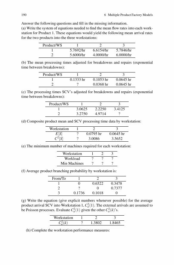
190 6 Multiple Product Factory Models
Answer the following questions and fill in the missing information.(a) Write the system of equations needed to find the mean flow rates into each work-station for Product 1. These equations would yield the following mean arrival ratesfor the two products into the three workstations:
Product/WS 1 2 31 5.7692/hr 6.6154/hr 5.7846/hr2 5.6000/hr 4.0000/hr 6.0000/hr
(b) The mean processing times adjusted for breakdowns and repairs (exponentialtime between breakdowns):
Product/WS 1 2 31 0.1333 hr 0.1053 hr 0.0645 hr2 ? 0.0368 hr 0.0645 hr
(c) The processing times SCV’s adjusted for breakdowns and repairs (exponentialtime between breakdowns):
Product/WS 1 2 31 3.0625 2.2250 3.41252 3.2750 4.9714 ?
(d) Composite product mean and SCV processing time data by workstation:
Workstation 1 2 3E[S] ? 0.0795 hr 0.0645 hrC2[S] ? 3.0086 3.5652
(e) The minimum number of machines required for each workstation:
Workstation 1 2 3Workload ? ? ?
Min Machines ? ? ?
(f) Average product branching probability by workstation is:
From/To 1 2 31 0 0.6522 0.34782 ? 0 0.73773 0.1736 0.1018 0
(g) Write the equation (give explicit numbers whenever possible) for the averageproduct arrival SCV into Workstation 1, C2
a(1). The external arrivals are assumed tobe Poisson processes. Evaluate C2
a(1) given the other C2a(k)’s.
Workstation 1 2 3C2
a(k) ? 1.3802 1.8465
(h) Complete the workstation performance measures:

Problems 191
Fig. 6.5a Process routing forProduct 1 for Problem 6.8
1/5
72/3
1/3
2/10
1/10
7/10
4/5
7/8
7/8
Fig. 6.5b Process routing forProduct 2 for Problem 6.8
Workstation CTq(k) CT (k) W IP(k)1 0.2533 hr 0.3757 hr 4.27142 ? ? ?3 0.5537 hr 0.6182 hr 7.2857
(i) What are the values of the factory system performance measures of cycle time(CTs), work-in-process (WIPs) and throughput?(j) What are the values of the individual product system performance measures ofthroughput and cycle time (CT i) for i = 1,2?
6.8. This problem is designed to encompasses all of the basic components of build-ing a multiple product model. To help reduce the time to solve the problem, manyof the numerical values are given so that the entire problem need not be workedout. There are ten parts to the problem with several tables of numerical values beinggiven; however, many of the tables will contain incomplete information, so thoseplaces in the table should be filled in.
A company is developing a factory to produce two different products. Both prod-ucts use three distinct machining processes; thus, the factory will require three work-stations. Company management would like to know several things about the factorybefore it is built. To support this analysis engineering has developed estimates forthe necessary product processing information. This information is listed below, andFigs. 6.5a and 6.5b depict the product processing routings. Answer the questionsand fill in the missing data.
Mean processing times by product and workstation.
Product/WS 1 2 3 41 7.2 min 6 min 9 min 7.2 min2 6 min 2.1 min 3.6 min
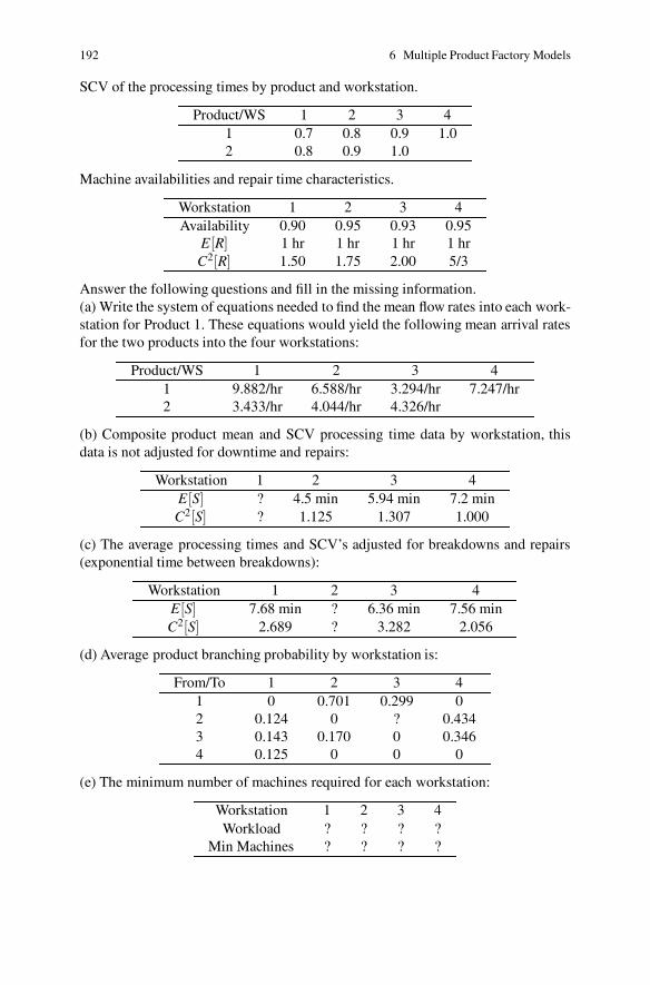
192 6 Multiple Product Factory Models
SCV of the processing times by product and workstation.
Product/WS 1 2 3 41 0.7 0.8 0.9 1.02 0.8 0.9 1.0
Machine availabilities and repair time characteristics.
Workstation 1 2 3 4Availability 0.90 0.95 0.93 0.95
E[R] 1 hr 1 hr 1 hr 1 hrC2[R] 1.50 1.75 2.00 5/3
Answer the following questions and fill in the missing information.(a) Write the system of equations needed to find the mean flow rates into each work-station for Product 1. These equations would yield the following mean arrival ratesfor the two products into the four workstations:
Product/WS 1 2 3 41 9.882/hr 6.588/hr 3.294/hr 7.247/hr2 3.433/hr 4.044/hr 4.326/hr
(b) Composite product mean and SCV processing time data by workstation, thisdata is not adjusted for downtime and repairs:
Workstation 1 2 3 4E[S] ? 4.5 min 5.94 min 7.2 minC2[S] ? 1.125 1.307 1.000
(c) The average processing times and SCV’s adjusted for breakdowns and repairs(exponential time between breakdowns):
Workstation 1 2 3 4E[S] 7.68 min ? 6.36 min 7.56 minC2[S] 2.689 ? 3.282 2.056
(d) Average product branching probability by workstation is:
From/To 1 2 3 41 0 0.701 0.299 02 0.124 0 ? 0.4343 0.143 0.170 0 0.3464 0.125 0 0 0
(e) The minimum number of machines required for each workstation:
Workstation 1 2 3 4Workload ? ? ? ?
Min Machines ? ? ? ?
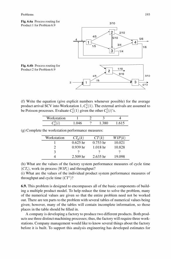
Problems 193
Fig. 6.6a Process routing forProduct 1 for Problem 6.9
1/4
44/5
1/5 3/4
2/10
3/10
5/6
1/6
5/10
2
4
3
1
Fig. 6.6b Process routing forProduct 2 for Problem 6.9
(f) Write the equation (give explicit numbers whenever possible) for the averageproduct arrival SCV into Workstation 1, C2
a(1). The external arrivals are assumed tobe Poisson processes. Evaluate C2
a(1) given the other C2a(i)’s.
Workstation 1 2 3 4C2
a(i) 1.046 ? 1.380 1.615
(g) Complete the workstation performance measures:
Workstation CTq(k) CT (k) W IP(k)1 0.625 hr 0.753 hr 10.0212 0.939 hr 1.018 hr 10.8283 ? ? ?4 2.509 hr 2.635 hr 19.098
(h) What are the values of the factory system performance measures of cycle time(CTs), work-in-process (WIPs) and throughput?(i) What are the values of the individual product system performance measures ofthroughput and cycle time (CT i)?
6.9. This problem is designed to encompasses all of the basic components of build-ing a multiple product model. To help reduce the time to solve the problem, manyof the numerical values are given so that the entire problem need not be workedout. There are ten parts to the problem with several tables of numerical values beinggiven; however, many of the tables will contain incomplete information, so thoseplaces in the table should be filled in.
A company is developing a factory to produce two different products. Both prod-ucts use three distinct machining processes; thus, the factory will require three work-stations. Company management would like to know several things about the factorybefore it is built. To support this analysis engineering has developed estimates for
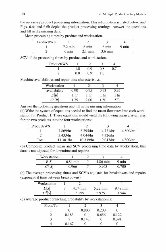
194 6 Multiple Product Factory Models
the necessary product processing information. This information is listed below, andFigs. 6.6a and 6.6b depict the product processing routings. Answer the questionsand fill in the missing data.
Mean processing times by product and workstation.
Product/WS 1 2 3 41 7.2 min 6 min 6 min 9 min2 6 min 2.1 min 3.6 min
SCV of the processing times by product and workstation.
Product/WS 1 2 3 41 1.0 0.9 0.8 0.72 0.8 0.9 1.0
Machine availabilities and repair time characteristics.
Workstation 1 2 3 4availability 0.90 0.95 0.93 0.95
E[R] 1 hr 1 hr 1 hr 1 hrC2[R] 1.75 2.00 1.50 5/3
Answer the following questions and fill in the missing information.(a) Write the system of equations needed to find the mean flow rates into each work-station for Product 1. These equations would yield the following mean arrival ratesfor the two products into the four workstations:
Product/WS 1 2 3 41 7.869/hr 6.295/hr 4.721/hr 4.800/hr2 3.433/hr 4.044/hr 4.326/hr
Total 11.301/hr 10.339/hr 9.047/hr 4.800/hr
(b) Composite product mean and SCV processing time data by workstation, thisdata is not adjusted for downtime and repairs:
Workstation 1 2 3 4E[S] 6.84 min ? 4.86 min 9 minC2[S] 0.966 ? 0.963 0.700
(c) The average processing times and SCV’s adjusted for breakdowns and repairs(exponential time between breakdowns):
Workstation 1 2 3 4E[S] ? 4.74 min 5.22 min 9.48 minC2[S] ? 3.155 2.975 1.544
(d) Average product branching probability by workstation is:
From/To 1 2 3 41 0 0.800 0.200 02 0.183 0 0.656 0.1223 ? 0.143 0 0.3914 0.167 0 0 0

Problems 195
(e) The minimum number of machines required for each workstation:
Workstation 1 2 3 4Workload ? ? ? ?
Min Machines ? ? ? ?
(f) Write the equation (give explicit numbers whenever possible) for the averageproduct arrival SCV into Workstation 1, C2
a(1). The external arrivals are assumed tobe Poisson processes. Evaluate C2
a(1) given the other C2a(k)’s.
Workstation 1 2 3 4C2
a(i) ? 1.602 1.841 1.497
(g) Complete the workstation performance measures:
Workstation CTq(i) CT (i) W IP(i)1 17.40 min 24.96 min 4.7032 48.24 min 52.98 min 9.1273 ? ? ?4 45.12 min 54.60 min 4.366
(h) What are the values of the factory system performance measures of cycle time(CTs), work-in-process (WIPs) and throughput?(i) What are the values of the individual product system performance measures ofthroughput and cycle time (CT i)?
6.10. Using a spreadsheet program such as Excel, solve Problem 6.1.
6.11. Using a spreadsheet program such as Excel, solve Problem 6.2.
6.12. A factory consists of five workstations and produces two products. Developthe product and factory performance measures of throughput, cycle time and work-in-process. Job Type 1 arrives according to a Poisson process with a mean rate of5 per hour and Job Type 2 arrives with a mean rate of 3 per hour and a squaredcoefficient of variation of the inter-arrival times of 2. There are two machines atWorkstation 2; all other workstations have only one machine. The process flow,mean processing times in hours, and squared coefficient of variation of the process-ing times are as follows:
Workstation Mean Service Time SCV Service Timeby Step # by Step # by Step #
Job Type 1 2 3 1 2 3 1 2 31 1 2 3 0.16 0.17 0.18 2.0 1.3 1.001 4 2 5 0.30 0.30 0.28 1.0 1.5 0.75
6.13. For the factory of Problem 6.12, the factory can be segmented into two cellularlines - one product manufactured in each line. Assuming that the mean processingtimes for Machine 2 can be reduced by 15% when the products are not processedon the same machine. That is, the workstation can specialize its setup operationby product type. Compute the product and total factory performance measures andcompare these with the composite factory organization computed in Problem 6.12.
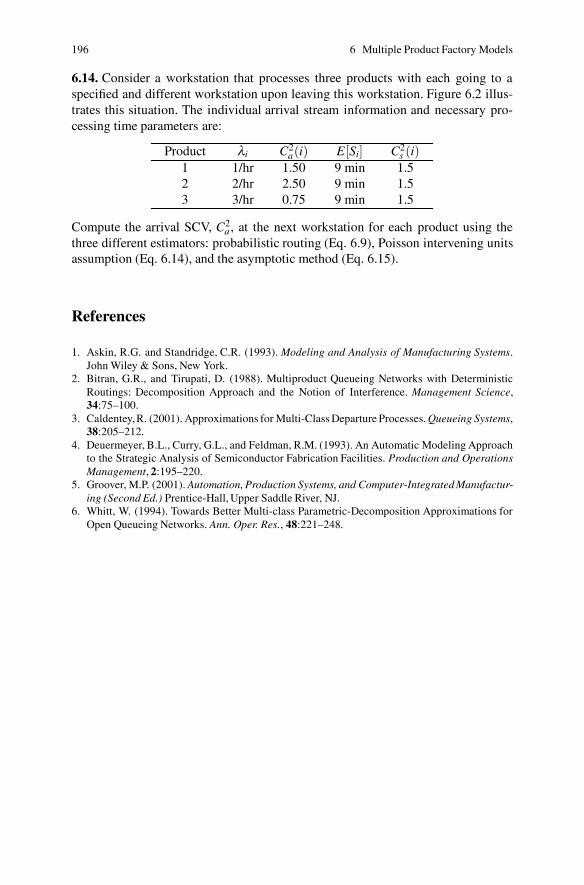
196 6 Multiple Product Factory Models
6.14. Consider a workstation that processes three products with each going to aspecified and different workstation upon leaving this workstation. Figure 6.2 illus-trates this situation. The individual arrival stream information and necessary pro-cessing time parameters are:
Product λi C2a(i) E[Si] C2
s (i)1 1/hr 1.50 9 min 1.52 2/hr 2.50 9 min 1.53 3/hr 0.75 9 min 1.5
Compute the arrival SCV, C2a , at the next workstation for each product using the
three different estimators: probabilistic routing (Eq. 6.9), Poisson intervening unitsassumption (Eq. 6.14), and the asymptotic method (Eq. 6.15).
References
1. Askin, R.G. and Standridge, C.R. (1993). Modeling and Analysis of Manufacturing Systems.John Wiley & Sons, New York.
2. Bitran, G.R., and Tirupati, D. (1988). Multiproduct Queueing Networks with DeterministicRoutings: Decomposition Approach and the Notion of Interference. Management Science,34:75–100.
3. Caldentey,R. (2001). Approximations for Multi-Class Departure Processes. Queueing Systems,38:205–212.
4. Deuermeyer, B.L., Curry, G.L., and Feldman, R.M. (1993). An Automatic Modeling Approachto the Strategic Analysis of Semiconductor Fabrication Facilities. Production and OperationsManagement, 2:195–220.
5. Groover, M.P. (2001). Automation, Production Systems, and Computer-Integrated Manufactur-ing (Second Ed.) Prentice-Hall, Upper Saddle River, NJ.
6. Whitt, W. (1994). Towards Better Multi-class Parametric-Decomposition Approximations forOpen Queueing Networks. Ann. Oper. Res., 48:221–248.
Chapter 7Models of Various Forms of Batching
Grouping individual jobs into sets, called batches, is a strategy frequently used inindustry. One cause of batching is for the purpose of transportation between work-stations. For instance, workers may require mechanical help for moving heavy itemsbetween two machines. If the mechanical help is a large machine such as a forklift,then a pallet might be loaded first before a forklift truck is requested. Another formof batching occurs when items are batched by type for the purpose of sharing amachine setup step even though the items are actually processed individually. Bybatching like items, only one setup need be performed for the whole set. And fi-nally, a frequently encountered batch service process is that of a multiple servicecapacity resource such as an oven. Due to the slow processing rates of some heat-treatment or plating processes, large capacity machines have been developed thatcan process several units of an item simultaneously.
The batching phenomenon is motivated by a perceived beneficial effect of group-ing. However, the impact on downstream processing stations can be significant. Toillustrate, consider the batch move concept where, say k, items are grouped togetherfor the convenience of moving them to a subsequent single unit processing station.Items will arrive at the next workstation k at a time, so the workstation might be idlefor a while and then instantaneously have a queue of waiting units. The variabilityof a batch arrival process when the batch is broken back into individuals (frequentlycaused by processing items simultaneously) is much greater than the inter-arrivalvariability of the individual items and, the workstation queueing behavior will beexacerbated. This leads to increased cycle times and larger WIP levels at the down-stream workstation. In addition, the batch process itself causes an increased delaybecause units must wait for the completion of other units before they can be groupedand continue processing.
In this chapter, models are developed for various forms of batching and so thatthe benefits and costs of the grouping process under consideration can be quanti-fied. For the setup sharing situation, there will be a trade-off between the cycle timeincrease and the setup time savings due to batching. The chapter is concluded witha discussion of network models that include a batch (oven-type) processing work-station. The term “job” can be confusing because in some contexts a job my refer
197

198 7 Models of Various Forms of Batching
Single Unit Server
Batch Forming
Queued Batches
Single Unit Server
Holding Area
Fig. 7.1 The batch move model structure: batches are formed after single unit processing and aretransported to the next workstation; batches wait in the queue until service on individual itemswithin the batch commences; finally, items leave as individuals as soon their processing has beencompleted
to an individual item and in other contexts it may refer to the entire batch. To avoidconfusion, the term “item” will always be used for an individual job and never tothe entire batch.
7.1 Batch Moves
Consider a situation where individual items are grouped together into fixed batchesof size k at the completion of processing at a workstation that processes single units.Items wait in the incomplete batch until the proper quantity has accrued and then thefull batch is transported to the next workstation. (A basic assumption used through-out this text is that transportation time is negligible and, therefore, is not explicitlyconsidered. If transportation time is significant, it can often be approximated in themodel by considering the transporter as a separate workstation.) An additional as-sumption is made that the receiving workstation processes items individually, hence,the batch is merely a convenient transportation tool. The modeling of the batch movesituation is a building block for more complex models. In addition, we will demon-strate that batch moves add to the cycle time in comparison to a system where itemsare moved individually. Figure 7.1 illustrates a batch move system.
To model the batch move, several aspects of the problem will have to be con-sidered. First, the batch forming time as it contributes to each individual item, orthe average item delay within a partial batch, needs to be computed. (The batchforming time is added to the cycle time of the workstation receiving the batch eventhough the batch forming actually takes place at the workstation sending the batch.)Then the arrival stream characteristics for the batch receiving workstation need bedeveloped; that is, the mean arrival rate for batches and the squared coefficient ofvariation of the inter-arrival batch times must be computed. And finally, the model-ing approach for developing the second workstation cycle time is different than ourprevious analyses. The cycle time model is separated into the standard componentsof the queue time and the service time. The queue time, however, is developed from
7.1 Batch Moves 199
the batch point of view. The individual item’s service time is the average time forprocessing individuals. These individuals are assumed to be released immediatelyafter processing to move on to their next workstation. But since there are k items inthe batch, the items have different delays while awaiting their turn at service. Thefirst item served from a batch has no additional delay due to waiting for others fromthe same batch, while the second item serviced from the batch waits for the firstitem, the third item waits for the first two selected items, and so on. The averagedelay is then taken over the composite delay for all items in the batch. These cycletime component analyses are addressed one at a time below.
7.1.1 Batch Forming Time
A batch is formed by grouping k individually arriving items together. Let Td be therandom variable denoting the time between departures from the source workstationthat are to be batched for transportation to the destination workstation. Note thatthe arrival rate of individuals λ (I), in the absence of batching, to the destinationworkstation is given by
λ (I) =1
E[Td ].
The random variable T (B) is the inter-arrival time of batches. This random variableis the sum of k individual inter-departure times
T (B) = Td,1 +Td,2 + · · ·+Td,k .
The individual inter-departure times Td,i for i = 1, · · · ,k are independent and iden-tically distributed (i.i.d.) random variables; thus, the expected value of the batchinter-arrival time is
E[T (B)] = kE[Td ] .
Hence, the arrival rate of batches to the destination workstation, λ (B), is
λ (B) =1
E[T (B)]=
1kE[Td ]
=λ (I)
k. (7.1)
The squared coefficient of variation, C2[T (B)], of the batch inter-arrival times atthe destination workstation is obtained from
C2[T(B)] =V [T (B)]E[T (B)]2
,
where the variance is computed from
V [T (B)] = V [Td,1 +Td,2 + · · ·+Td,k] = kV [Td ] ,
200 7 Models of Various Forms of Batching
since the inter-departure random variables are assumed independent (see Prop-erty 1.6 or Eq. 1.25). Thus, the squared coefficient of variation of the batch inter-arrival times can be computed from the squared coefficient of variation of the indi-vidual inter-arrival times by
C2[T (B)] =V [T (B)]E[T (B)]2
=kV [Td ]
(kE[Td ])2 =C2[Td]
k. (7.2)
The delay that an individual item encounters when being placed into a batchdepends on where it is among the k batched items. The first departing item used tostart the formation of a new batch must wait for k−1 more items to depart before thebatch has been formed and released for transportation to the destination workstation.Denote this delay by the random variable D1 where
D1 = Td,2 + · · ·+Td,k .
The second item forming the new batch has to wait for k−2 succeeding departuresand its waiting time is the random variable D2 given by
D2 = Td,3 + · · ·+Td,k .
The other items in the batch have delay times similarly developed with the lastitem encountering no delay (i.e., Dk = 0). The last item’s arrival signals the batch iscomplete and the batch is instantaneously transported to the destination workstation.The average delay encountered by an item in the batch is then the expected value ofthe sum of all these delays divided by the batch size k; that is,
E[D] =E[D1 +D2 + · · ·+Dk−1 +Dk]
k
=(k−1)E[Td ]+ (k−2)E[Td ]+ · · ·+1E[Td ]+0E[Td]
k
=((k−1)k/2)E[Td ]
k
=(k−1)
2E[Td ] . (7.3)
Thus, the average delay encountered by an individual item when waiting for a batchof size k to form is (k−1)E[Td ]/2.
One should recognize that the term E[Td] in the expected batch waiting time perindividual is the time between arrivals for the particular situation that was used tomotivate this analysis. In this situation, batching after job completion at a worksta-tion is done for the purpose of transporting the items to the next workstation. Thebatching operation could occur at the front of a batch service workstation such asan oven. In this case, the average delay would follow the same form as the resultjust derived, but the individual item’s inter-arrival time would then be denoted as
7.1 Batch Moves 201
E[Ta]. This is the expected time between arrivals to the workstation and, therefore,the inter-arrival time for batch items.
The batching form that has been analyzed is for a single product or for indis-criminate grouping of multiple products. It is very likely that batching is restrictedto jobs of the same type. In this situation, then multiple batch types can be formingsimultaneously and the wait associated with batch formation of a given item typewould be a function of the inter-arrival time to the workstation of that job type.
7.1.2 Batch Queue Cycle Time
Modeling the cycle time for the recipient workstation for the batch move situationhas two distinct components: the queue time and the service time. The queueingdelay is modeled from the batch units point of view. The items within a batch seethis queueing phenomenon as batches waiting and then moving up in the line basedon batches being served. The arrival rate to this queue is λ (B) with correspondingsquared coefficient of variation C2[T (B)]. It may be clearer to denote the randomvariable T (B) as Ta(B) to distinguish and relate this random variable with the indi-vidual inter-arrival time random variable Ta(I).
The service time that these batches observe while they wait in the queue is forbatches (they move forward one location in the queue whenever a batch has beencompletely served). The service time for these batches is the time it takes the serverto process all of the items within the batch being served, which is the random vari-able Ts(B) given by
Ts(B) = Ts,1(I)+Ts,2(I)+ · · ·+Ts,k(I) ,
where the (B) and (I) notation again stands for batches and individuals, respectively.Note that since this is a single item service facility (items are processed one at atime), the processing times Ts,i(I) are independent and identically distributed ran-dom variables with known mean E[Ts(I)] and known squared coefficient of variationC2[Ts(I)]. Thus, the (perceived) batch service time characteristics can be computedfrom these known individual item data as
E[Ts(B)] = kE[Ts(I)] ,
C2[Ts(B)] =C2[Ts(I)]
k.
The G/G/1 cycle time approximation model is used to compute the cycle timein the queue for the waiting batches. The utilization factor for the workstation mustalso be computed for batches. This computation is
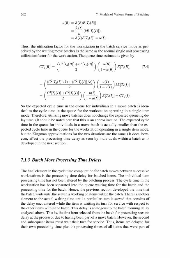
202 7 Models of Various Forms of Batching
u(B) = λ (B)E[Ts(B)]
=λ (I)
k(kE[Ts(I)])
= λ (I)E[Ts(I)] = u(I) .
Thus, the utilization factor for the workstation in the batch service mode as per-ceived by the waiting move batches is the same as the normal single unit processingutilization factor for the workstation. The queue time estimate is given by
CTq(B) =(
C2[Ta(B)]+C2[Ts(B)]2
)(
u(B)1−u(B)
)
E[Ts(B)] (7.4)
=(
(C2[Ta(I)]/k)+(C2[Ts(I)]/k)2
)(
u(I)1−u(I)
)
kE[Ts(I)]
=(
C2[Ta(I)]+C2[Ts(I)]2
)(
u(I)1−u(I)
)
E[Ts(I)] = CTq(I) .
So the expected cycle time in the queue for individuals in a move batch is iden-tical to the cycle time in the queue for the workstation operating in a single itemmode. Therefore, utilizing move batches does not change the expected queueing de-lay time. (It should be noted here that this is an approximation. The expected cycletime in the queue for individuals in a move batch is actually smaller than the ex-pected cycle time in the queue for the workstation operating in a single item mode,but the Kingman approximations for the two situations are the same.) It does, how-ever, affect the processing time delay as seen by individuals within a batch as isdeveloped in the next section.
7.1.3 Batch Move Processing Time Delays
The final element in the cycle time computation for batch moves between successiveworkstations is the processing time delay for batched items. The individual itemprocessing time has not been altered by the batching process. The cycle time in theworkstation has been separated into the queue waiting time for the batch and theprocessing time for the batch. Hence, the previous section developed the time thatthe batch waits until the server is working on items within the batch. There is anotherelement to the actual waiting time until a particular item is served that consists ofthe delay encountered while the item is waiting its turn for service with respect tothe other items within the batch. This delay is analogous to the batch forming delayanalyzed above. That is, the first item selected from the batch for processing sees nodelay at the processor due to having been part of a move batch. However, the secondand subsequent items must wait their turn for service. Thus, items are delayed fortheir own processing time plus the processing times of all items that were part of
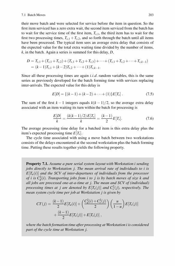
7.1 Batch Moves 203
their move batch and were selected for service before the item in question. So thefirst item serviced has a zero extra wait, the second item serviced from the batch hasto wait for the service time of the first item, Ts,1, the third item has to wait for thefirst two processing times, Ts,1 +Ts,2, and so forth through the batch until all itemshave been processed. The typical item sees an average extra delay that consists ofthe expected value for the total extra waiting time divided by the number of items,k, in the batch. Again a series is summed for this delay, D,
D = Ts,1 +(Ts,1 +Ts,2)+(Ts,1 +Ts,2 +Ts,3)+ · · ·+(Ts,1 +Ts,2 + · · ·+Ts,k−1)= (k−1)Ts,1 +(k−2)Ts,2 + · · ·+(1)Ts,k−1.
Since all these processing times are again i.i.d. random variables, this is the sameseries as previously developed for the batch forming time with services replacinginter-arrivals. The expected value for this delay is
E[D] = {(k−1)+(k−2)+ · · ·+(1)}E[Ts] . (7.5)
The sum of the first k− 1 integers equals k(k − 1)/2, so the average extra delayassociated with an item waiting its turn within the batch for processing is
E[D]k
=(k(k−1)/2)E[Ts]
k=
(k−1)2
E[Ts]. (7.6)
The average processing time delay for a batched item is this extra delay plus theitem’s expected processing time E[Ts].
The cycle time associated with using a move batch between two workstationsconsists of the delays encountered at the second workstation plus the batch formingtime. Putting these results together yields the following property.
Property 7.1. Assume a pure serial system layout with Workstation i sendingjobs directly to Workstation j. The mean arrival rate of individuals to i isE[Ta(i)] and the SCV of inter-departures of individuals from the processorof i is C2
d(i). Transporting jobs from i to j is by batch moves of size k andall jobs are processed one-at-a-time at j. The mean and SCV of (individual)processing times at j are denoted by E[Ts( j)] and C2
s ( j), respectively. Themean system cycle time per job at Workstation j is given by
CT ( j) =(k−1)
2E[Ta(i)]+
(
C2d(i)+C2
s ( j)2
)(
u1−u
)
E[Ts( j)]
+(k−1)
2E[Ts( j)]+E[Ts( j)] ,
where the batch formation time after processing at Workstation i is consideredpart of the cycle time at Workstation j.
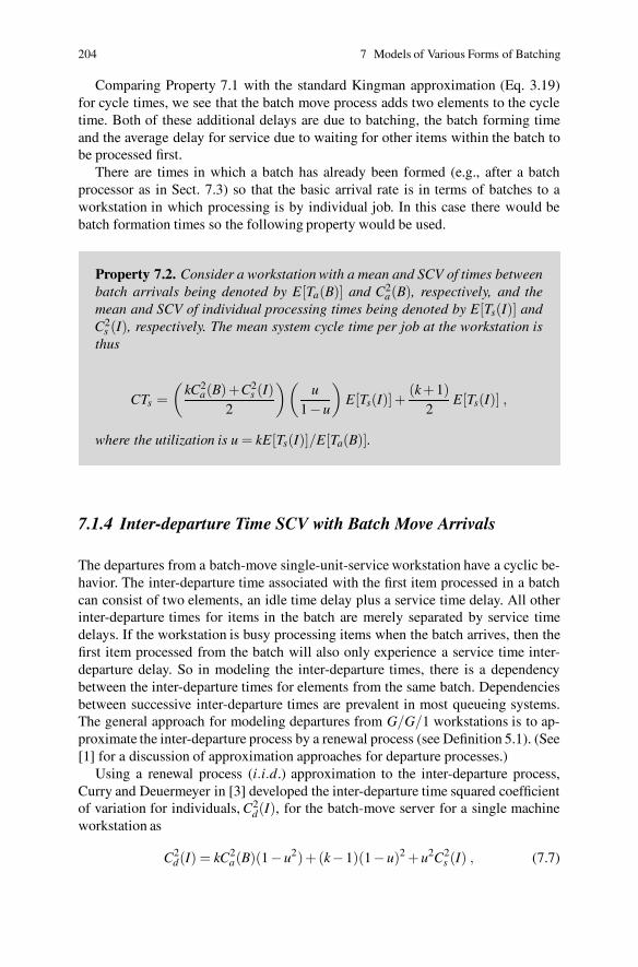
204 7 Models of Various Forms of Batching
Comparing Property 7.1 with the standard Kingman approximation (Eq. 3.19)for cycle times, we see that the batch move process adds two elements to the cycletime. Both of these additional delays are due to batching, the batch forming timeand the average delay for service due to waiting for other items within the batch tobe processed first.
There are times in which a batch has already been formed (e.g., after a batchprocessor as in Sect. 7.3) so that the basic arrival rate is in terms of batches to aworkstation in which processing is by individual job. In this case there would bebatch formation times so the following property would be used.
Property 7.2. Consider a workstation with a mean and SCV of times betweenbatch arrivals being denoted by E[Ta(B)] and C2
a(B), respectively, and themean and SCV of individual processing times being denoted by E[Ts(I)] andC2
s (I), respectively. The mean system cycle time per job at the workstation isthus
CTs =(
kC2a(B)+C2
s (I)2
)(
u1−u
)
E[Ts(I)]+(k+1)
2E[Ts(I)] ,
where the utilization is u = kE[Ts(I)]/E[Ta(B)].
7.1.4 Inter-departure Time SCV with Batch Move Arrivals
The departures from a batch-move single-unit-service workstation have a cyclic be-havior. The inter-departure time associated with the first item processed in a batchcan consist of two elements, an idle time delay plus a service time delay. All otherinter-departure times for items in the batch are merely separated by service timedelays. If the workstation is busy processing items when the batch arrives, then thefirst item processed from the batch will also only experience a service time inter-departure delay. So in modeling the inter-departure times, there is a dependencybetween the inter-departure times for elements from the same batch. Dependenciesbetween successive inter-departure times are prevalent in most queueing systems.The general approach for modeling departures from G/G/1 workstations is to ap-proximate the inter-departure process by a renewal process (see Definition 5.1). (See[1] for a discussion of approximation approaches for departure processes.)
Using a renewal process (i.i.d.) approximation to the inter-departure process,Curry and Deuermeyer in [3] developed the inter-departure time squared coefficientof variation for individuals, C2
d(I), for the batch-move server for a single machineworkstation as
C2d(I) = kC2
a(B)(1−u2)+(k−1)(1−u)2 +u2C2s (I) , (7.7)
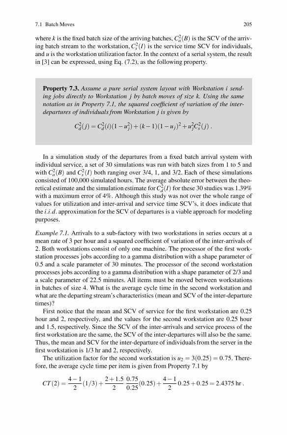
7.1 Batch Moves 205
where k is the fixed batch size of the arriving batches, C2a(B) is the SCV of the arriv-
ing batch stream to the workstation, C2s (I) is the service time SCV for individuals,
and u is the workstation utilization factor. In the context of a serial system, the resultin [3] can be expressed, using Eq. (7.2), as the following property.
Property 7.3. Assume a pure serial system layout with Workstation i send-ing jobs directly to Workstation j by batch moves of size k. Using the samenotation as in Property 7.1, the squared coefficient of variation of the inter-departures of individuals from Workstation j is given by
C2d( j) = C2
d(i)(1−u2j)+(k−1)(1−u j)2 +u2
jC2s ( j) .
In a simulation study of the departures from a fixed batch arrival system withindividual service, a set of 30 simulations was run with batch sizes from 1 to 5 andwith C2
a(B) and C2s (I) both ranging over 3/4, 1, and 3/2. Each of these simulations
consisted of 100,000 simulated hours. The average absolute error between the theo-retical estimate and the simulation estimate for C2
d(I) for these 30 studies was 1.39%with a maximum error of 4%. Although this study was not over the whole range ofvalues for utilization and inter-arrival and service time SCV’s, it does indicate thatthe i.i.d. approximation for the SCV of departures is a viable approach for modelingpurposes.
Example 7.1. Arrivals to a sub-factory with two workstations in series occurs at amean rate of 3 per hour and a squared coefficient of variation of the inter-arrivals of2. Both workstations consist of only one machine. The processor of the first work-station processes jobs according to a gamma distribution with a shape parameter of0.5 and a scale parameter of 30 minutes. The processor of the second workstationprocesses jobs according to a gamma distribution with a shape parameter of 2/3 anda scale parameter of 22.5 minutes. All items must be moved between workstationsin batches of size 4. What is the average cycle time in the second workstation andwhat are the departing stream’s characteristics (mean and SCV of the inter-departuretimes)?
First notice that the mean and SCV of service for the first workstation are 0.25hour and 2, respectively, and the values for the second workstation are 0.25 hourand 1.5, respectively. Since the SCV of the inter-arrivals and service process of thefirst workstation are the same, the SCV of the inter-departures will also be the same.Thus, the mean and SCV for the inter-departure of individuals from the server in thefirst workstation is 1/3 hr and 2, respectively.
The utilization factor for the second workstation is u2 = 3(0.25) = 0.75. There-fore, the average cycle time per item is given from Property 7.1 by
CT (2) =4−1
2(1/3)+
2 +1.52
0.750.25
(0.25)+4−1
20.25 +0.25 = 2.4375 hr .
206 7 Models of Various Forms of Batching
The mean departure rate of individuals equals the mean arrival rate of individualswhich is 3 per hour. The squared coefficient of variation of the inter-departure timesis approximated from Property 7.3 by
C2d(2) = 2(1−0.752)+3(1−0.75)2 +0.752(1.5) = 1.9063 .
��
• Suggestion: Do Problems 7.1 and 7.2.
7.2 Batching for Setup Reduction
The Batch Move Model of Sect. 7.1 was developed to model situations where in-dividual items are batched together for the purpose of transporting them simultane-ously to the next workstation. A similar situation exists when a single-unit process-ing workstation must be setup immediately before a group (or batch) of items of thesame job type are to be processed on the machine. Frequently, this setup operationuses a significant amount of time and this can make it inefficient or even infeasibleto run single unit batches. For this situation, the batching operation can be thoughtof as occurring at the front of this workstation rather than at the end the predeces-sor workstation. Accordingly, the batch forming time will be accounted for in thisworkstation. The reason for forming a batch of say size k is to spread the batch setuptime across k jobs rather than one job. Hence, if the setup time for a certain classof items is one hour, then if these items are run “one-at-a-time” each one wouldadd essentially one hour to their processing time. If this type of item is processedin batches of size 4, then the one hour setup time would be required only once forthe batch, essentially adding 1/4 hour of setup time to each item processed insteadof one hour. Thus, there are many choices for the batch size for each item and abatch quantity should be chosen that balances the setup time reduction against theincreased batching delay as the batching quantity is increased. If there is only oneitem type, then the optimal batch size can be found by searching over the single pa-rameter k. Of course, if there really is only one item type, the machine would alwaysbe left setup for that type and then there would not be a setup time balancing prob-lem, unless recalibration, cleaning, or similar operation is periodically required, andthis operation would usually specify the batch size k. Most realistic problems in-volving setups consist of at least two job types where processing alternates betweentypes.
There are at least two different procedures possible in forming the batches. Onemethod would be to form the batch as the individuals arrive to the workstation andanother method would be to form the batch just before processing. The procedureused would depend on the physical properties of the jobs and the machining re-quirements. For simplicity, we will assume the first procedure, that is, batches forprocessing are formed as the individual jobs arrive to the workstation. We shall also
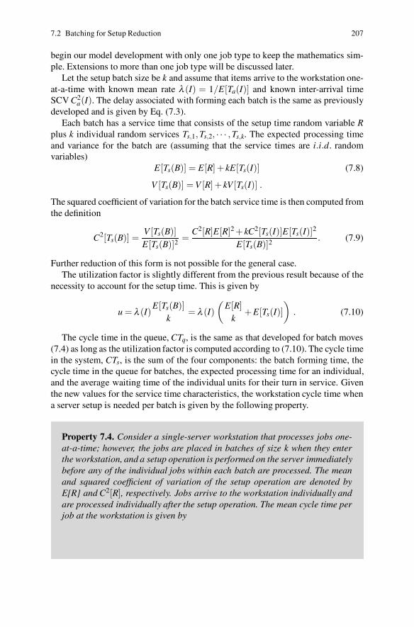
7.2 Batching for Setup Reduction 207
begin our model development with only one job type to keep the mathematics sim-ple. Extensions to more than one job type will be discussed later.
Let the setup batch size be k and assume that items arrive to the workstation one-at-a-time with known mean rate λ (I) = 1/E[Ta(I)] and known inter-arrival timeSCV C2
a(I). The delay associated with forming each batch is the same as previouslydeveloped and is given by Eq. (7.3).
Each batch has a service time that consists of the setup time random variable Rplus k individual random services Ts,1,Ts,2, · · · ,Ts,k. The expected processing timeand variance for the batch are (assuming that the service times are i.i.d. randomvariables)
E[Ts(B)] = E[R]+ kE[Ts(I)] (7.8)
V [Ts(B)] = V [R]+ kV [Ts(I)] .
The squared coefficient of variation for the batch service time is then computed fromthe definition
C2[Ts(B)] =V [Ts(B)]E[Ts(B)]2
=C2[R]E[R]2 + kC2[Ts(I)]E[Ts(I)]2
E[Ts(B)]2. (7.9)
Further reduction of this form is not possible for the general case.The utilization factor is slightly different from the previous result because of the
necessity to account for the setup time. This is given by
u = λ (I)E[Ts(B)]
k= λ (I)
(
E[R]k
+E[Ts(I)])
. (7.10)
The cycle time in the queue, CTq, is the same as that developed for batch moves(7.4) as long as the utilization factor is computed according to (7.10). The cycle timein the system, CTs, is the sum of the four components: the batch forming time, thecycle time in the queue for batches, the expected processing time for an individual,and the average waiting time of the individual units for their turn in service. Giventhe new values for the service time characteristics, the workstation cycle time whena server setup is needed per batch is given by the following property.
Property 7.4. Consider a single-server workstation that processes jobs one-at-a-time; however, the jobs are placed in batches of size k when they enterthe workstation, and a setup operation is performed on the server immediatelybefore any of the individual jobs within each batch are processed. The meanand squared coefficient of variation of the setup operation are denoted byE[R] and C2[R], respectively. Jobs arrive to the workstation individually andare processed individually after the setup operation. The mean cycle time perjob at the workstation is given by
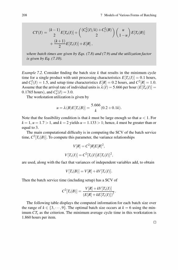
208 7 Models of Various Forms of Batching
CT(I) =(k−1)
2E[Ta(I)]+
(
(C2a(I)/k)+C2
s (B)2
)(
u1−u
)
E[Ts(B)]
+(k+1)
2E[Ts(I)]+E[R] ,
where batch times are given by Eqs. (7.8) and (7.9) and the utilization factoris given by Eq. (7.10).
Example 7.2. Consider finding the batch size k that results in the minimum cycletime for a single product with unit processing characteristics E[Ts(I)] = 0.1 hours,and C2
s (I) = 1.5, and setup time characteristics E[R] = 0.2 hours, and C2[R] = 1.0.Assume that the arrival rate of individual units is λ (I) = 5.666 per hour (E[Ta(I)] =0.1765 hours), and C2
a(I) = 3.0.The workstation utilization is given by
u = λ (B)E[Ts(B)] =5.666
k(0.2 +0.1k).
Note that the feasibility condition is that k must be large enough so that u < 1. Fork = 1, u = 1.7 > 1, and k = 2 yields u = 1.133 > 1; hence, k must be greater than orequal to 3.
The main computational difficulty is in computing the SCV of the batch servicetime, C2[Ts(B)]. To compute this parameter, the variance relationships
V [R] = C2[R]E[R]2,
V [Ts(I)] = C2[Ts(I)]E[Ts(I)]2,
are used, along with the fact that variances of independent variables add, to obtain
V [Ts(B)] = V [R]+ kV [Ts(I)].
Then the batch service time (including setup) has a SCV of
C2[Ts(B)] =V [R]+ kV [Ts(I)]
(E[R]+ kE[Ts(I)])2 .
The following table displays the computed information for each batch size overthe range of k ∈ {3, · · · ,9}. The optimal batch size occurs at k = 6 using the min-imum CTs as the criterion. The minimum average cycle time in this workstation is1.860 hours per item.
��

7.3 Batch Service Model 209
Table 7.1 Data for varying batch sizes for Example 7.2
k u E [Ts(B)] C2[Ts(B)] CTs
3 0.944 0.5 0.340 6.2544 0.850 0.6 0.278 2.4605 0.793 0.7 0.235 1.9746 0.755 0.8 0.203 1.8607 0.728 0.9 0.179 1.8638 0.708 1.0 0.160 1.9179 0.692 1.1 0.145 1.998
7.2.1 Inter-departure Time SCV with Batch Setups
The squared coefficient of variation of the inter-departure times for the workstationwith batch setups can be approximated by an i.i.d. departure model. We again referto [3] for the departure model as given in the following property.
Property 7.5. The squared coefficient of variation for the inter-departuretimes from a workstation that processes jobs one-at-a-time with a batch set-upis
C2[Td(I)] = kC2[Ta(B)](1−u2)+ k(1−u)2−1 +2k(1−u)(E[R]+E[Ts(I)])
E[Ta(B)]+
k(E[R]2(C2[R]+1)+ kE[Ts(I)]2(C2[Ts(I)]+1)+2E[R]E[Ts(I)])(E[Ta(B)])2 ,
where the notation is the same as in Property 7.4.
To illustrate the accuracy of this approximation, consider the case for k = 4 ofthe previous table. A simulation of this case, using 567,715 observations for the in-dividual inter-departure times yielded a mean value of C2[Td(I)] = 2.225 with thei.i.d. approximation being 2.2037, equation 7.11, which is less than -1.0% off of themeasured value. The measured value for C2[Ts(B)] was 0.279 versus the computedvalue of 0.278.
• Suggestion: Do Problem 7.3.
7.3 Batch Service Model
A batch server is a processor that can process several jobs simultaneously. Ovensand metal plating operations are examples, and this is the type of operation that isanalyzed in this section. Namely, we consider a batch server model where a fixed

210 7 Models of Various Forms of Batching
number of items are loaded and processed at the same time. Processing is not starteduntil the number of units in the batch, say k, are available. The batch is then loadedand held in the server for the allotted time. At the completion of service, the batchis removed from the server and the units either as a group or individually are sentto their next workstation. Different types of items may be grouped together or thebatching operation may be restricted to item specific groups.
7.3.1 Cycle Time for Batch Service
The arrival rate for batches and the associated squared coefficient of variation ofinter-arrival times of the batches, as they are related to the individual flow charac-teristics, were developed in Sect. 7.1.1. The modeling approach for a general arrivaland general service situation is to utilize the G/G/1 cycle time approximation, usingbatch timing characteristics in place of individual item information. Previously theadjustment equations for batch arrival data were developed given individual inter-arrival time information. These relationships are
λ (B) =λ (I)
k=
1kE[Ta(I)]
, (7.11)
C2[Ta(B)] =C2[Ta(I)]
k. (7.12)
The service time data, namely E[Ts(B)] and C2[Ts(B)], are characteristics of thejob and processor and so are known data. The workstation cycle time for batchprocessing is given by the following property.
Property 7.6. Consider a single-server workstation that processes jobs infixed batches of size k. Jobs arrive to the workstation individually. Upon enter-ing the workstation, the individual jobs are placed in batches before proceed-ing into the workstation. Service cannot start until a full batch is available.The mean and SCV of batch processing times are denoted by E[Ts(B)] andC2
s (B), respectively. The mean system cycle time per job at the workstation isgiven by
CTs =(k−1)
2E[Ta(I)]+E[Ts(B)]
+(
C2[Ta(B)]+C2[Ts(B)]2
)(
u(B)1−u(B)
)
E[Ts(B)] ,
where the utilization factor, u(B), is computed as u(B) = λ (B)E[Ts(B)].
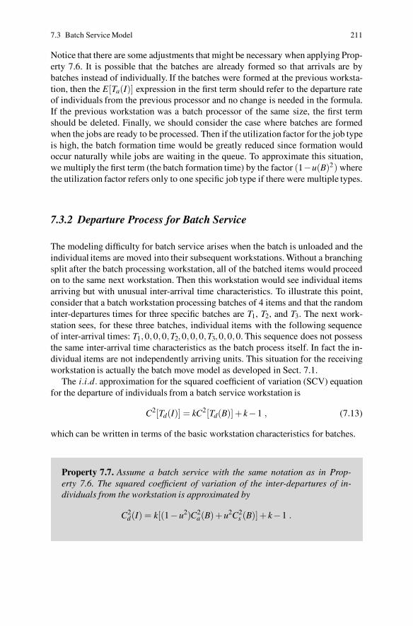
7.3 Batch Service Model 211
Notice that there are some adjustments that might be necessary when applying Prop-erty 7.6. It is possible that the batches are already formed so that arrivals are bybatches instead of individually. If the batches were formed at the previous worksta-tion, then the E[Ta(I)] expression in the first term should refer to the departure rateof individuals from the previous processor and no change is needed in the formula.If the previous workstation was a batch processor of the same size, the first termshould be deleted. Finally, we should consider the case where batches are formedwhen the jobs are ready to be processed. Then if the utilization factor for the job typeis high, the batch formation time would be greatly reduced since formation wouldoccur naturally while jobs are waiting in the queue. To approximate this situation,we multiply the first term (the batch formation time) by the factor (1−u(B)2) wherethe utilization factor refers only to one specific job type if there were multiple types.
7.3.2 Departure Process for Batch Service
The modeling difficulty for batch service arises when the batch is unloaded and theindividual items are moved into their subsequent workstations. Without a branchingsplit after the batch processing workstation, all of the batched items would proceedon to the same next workstation. Then this workstation would see individual itemsarriving but with unusual inter-arrival time characteristics. To illustrate this point,consider that a batch workstation processing batches of 4 items and that the randominter-departures times for three specific batches are T1, T2, and T3. The next work-station sees, for these three batches, individual items with the following sequenceof inter-arrival times: T1,0,0,0,T2,0,0,0,T3,0,0,0. This sequence does not possessthe same inter-arrival time characteristics as the batch process itself. In fact the in-dividual items are not independently arriving units. This situation for the receivingworkstation is actually the batch move model as developed in Sect. 7.1.
The i.i.d. approximation for the squared coefficient of variation (SCV) equationfor the departure of individuals from a batch service workstation is
C2[Td(I)] = kC2[Td(B)]+ k−1 , (7.13)
which can be written in terms of the basic workstation characteristics for batches.
Property 7.7. Assume a batch service with the same notation as in Prop-erty 7.6. The squared coefficient of variation of the inter-departures of in-dividuals from the workstation is approximated by
C2d(I) = k[(1−u2)C2
a(B)+u2C2s (B)]+ k−1 .

212 7 Models of Various Forms of Batching
Although Property 7.7 gives an SCV for the renewal process (Definition 5.1) ap-proximating the departure process, observe that the process formed by individualdepartures of a batch operation is clearly not a renewal process so that modeling thenext workstation could be problematic. This is the topic of the next section.
Property 7.7 illustrates that after a batch service, the process of separating thebatch into individual items causes the squared coefficient of variation to increasesignificantly as a function of the batch size parameter k. One would expect the mul-tiplication of C2[Td(B)] by the batch size k since this reverses the batching processadjustment. However, the additional factor k − 1 indicates that the batch processchanges the system’s flow characteristics significantly. Again this SCV approxima-tion ignores any dependencies in the inter-departure stream and treats each item’sinter-departure time as independent and identically distributed.
Example 7.3. Consider a batch-processing workstation in which arrivals to theworkstation are from another batch server so that the arrivals occur in batches ofsize 5 with a mean rate of 3 batches per hour and an SCV of batch inter-arrivaltimes of 0.75. The SCV of the batch service time is also 0.75 with a workstationload factor or utilization of 84%. The average time each job spends in the worksta-tion is thus given by
CT = 16.8 +0.75 +0.75
2× 0.84
1−0.84×16.8 = 82.95 min .
Note that 16.8 is the service time given in minutes and is obtained by dividing theutilization factor by the arrival rate. In addition, the first term in the cycle timeequation of Property 7.6 was not used since the arrivals were already in batches.
Since the SCV of the inter-arrival times and the service times are the same, itis also the SCV of the inter-departure times for batches. The approximation for theinter-departure SCV of individuals is given by
C2d(I) = 5
[
(1−0.842)(0.75)+0.842(0.75)]
+4 = 7.75.
��
Although the SCV calculation of 7.75 of inter-departures of Example 7.3 maygive an accurate representation of the actual departure stream, there are major prob-lems when using this value in a cycle time calculation for the downstream worksta-tion. The next section discusses how to better utilize batch output when modelingdownstream workstations.
• Suggestion: Do Problems 7.4–7.6.

7.4 Modeling the Workstation Following a Batch Server 213
7.4 Modeling the Workstation Following a Batch Server
Since the unbatching process after a batch-service workstation does not producea renewal process (i.e., a stream of inter-departure times that are independent andidentically distributed), it is prudent to model the recipient workstation as having abatch arrival process. This approach captures the true behavior of the arrival streamincluding the inter-dependence between arrivals, whereas the i.i.d. SCV approxima-tion does not. The analysis of the workstation depends on whether the jobs leavingthe batch processor are sent directly to the next workstation or if a probabilisticbranch follows the batch server.
7.4.1 A Serial System Topology
To illustrate the difficulties inherent in modeling the workstation following a batchservice operation, reconsider Example 7.3 and assume that the workstation of thatexample feeds into a workstation that processes jobs one-at-a-time. This down-stream workstation has a service process described by an exponential distributionwith a mean of 3 minutes. The workstation of Example 7.3 is feeding batches ofsize 5 to our workstation at a mean rate of 3 batches per hour with an SCV of batchinter-arrival times of 0.75 and an SCV of 7.75 of individuals. The workstation uti-lization factor is u = 5× 3× 0.05 = 0.75. Then using the standard approximationfor individuals, the system cycle time for this workstation is
CT =7.75 +1
2× 0.75
1−0.75×0.05 +0.05 = 0.706 hr . (7.14)
Simulating this situation yielded a cycle time estimate of 0.496 hours based onjust over 135,000 simulated services. The resultant inter-arrival stream characteris-tics were measured as E[Ta(I)] = 0.333, with C2[Ta(B)] = 0.753. The workstationutilization factor was measured to be 0.749. This data was from a simulation runlength of 10,000 hours with a statistics reset after 1,000 hours. So even though thefirst two moments of the inter-arrival time distribution were very accurate, the cycletime approximation was off by 42%. Why? The answer is in the arrival stream’scharacteristics. The first two moments of the inter-arrival time distribution does notcapture the grouping behavior observed in the batch arrival process. For example, itis quite possible to have an arrival stream sequence of batches of size 2 with exactlythe same mean and SCV; thus, it is clear that the first two moments alone cannotadequately describe an arrival process of individuals that arise from batches.
To properly take the arrival stream’s characteristics into account, the next work-station after the batch server workstation should be modeled as a batch arrival sta-tion, using the modeling approach detailed in Sect. 7.1 dealing with batch moves,specifically, Property 7.2 should be used. This approach treats the system as a batcharrival and batch server system for the queue time estimate and then adds the in-
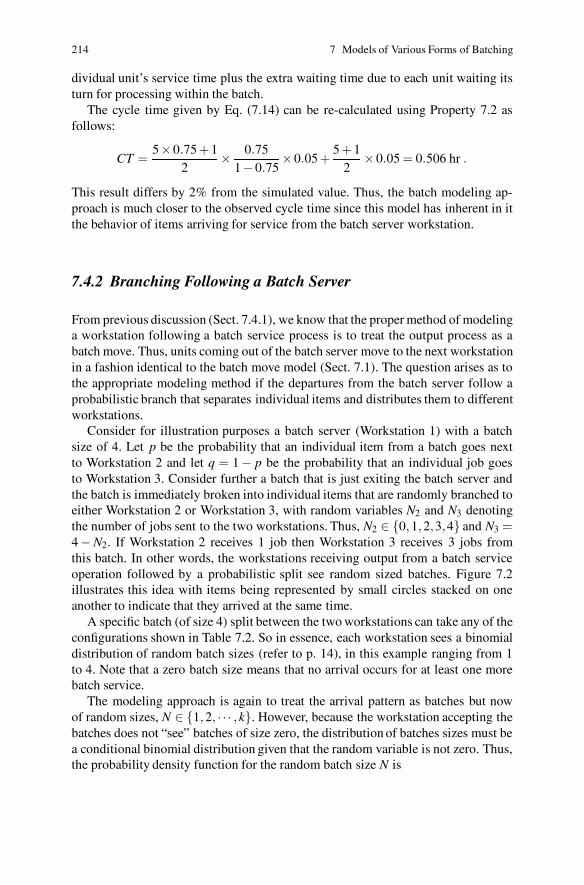
214 7 Models of Various Forms of Batching
dividual unit’s service time plus the extra waiting time due to each unit waiting itsturn for processing within the batch.
The cycle time given by Eq. (7.14) can be re-calculated using Property 7.2 asfollows:
CT =5×0.75 +1
2× 0.75
1−0.75×0.05 +
5 +12
×0.05 = 0.506 hr .
This result differs by 2% from the simulated value. Thus, the batch modeling ap-proach is much closer to the observed cycle time since this model has inherent in itthe behavior of items arriving for service from the batch server workstation.
7.4.2 Branching Following a Batch Server
From previous discussion (Sect. 7.4.1), we know that the proper method of modelinga workstation following a batch service process is to treat the output process as abatch move. Thus, units coming out of the batch server move to the next workstationin a fashion identical to the batch move model (Sect. 7.1). The question arises as tothe appropriate modeling method if the departures from the batch server follow aprobabilistic branch that separates individual items and distributes them to differentworkstations.
Consider for illustration purposes a batch server (Workstation 1) with a batchsize of 4. Let p be the probability that an individual item from a batch goes nextto Workstation 2 and let q = 1− p be the probability that an individual job goesto Workstation 3. Consider further a batch that is just exiting the batch server andthe batch is immediately broken into individual items that are randomly branched toeither Workstation 2 or Workstation 3, with random variables N2 and N3 denotingthe number of jobs sent to the two workstations. Thus, N2 ∈ {0,1,2,3,4} and N3 =4−N2. If Workstation 2 receives 1 job then Workstation 3 receives 3 jobs fromthis batch. In other words, the workstations receiving output from a batch serviceoperation followed by a probabilistic split see random sized batches. Figure 7.2illustrates this idea with items being represented by small circles stacked on oneanother to indicate that they arrived at the same time.
A specific batch (of size 4) split between the two workstations can take any of theconfigurations shown in Table 7.2. So in essence, each workstation sees a binomialdistribution of random batch sizes (refer to p. 14), in this example ranging from 1to 4. Note that a zero batch size means that no arrival occurs for at least one morebatch service.
The modeling approach is again to treat the arrival pattern as batches but nowof random sizes, N ∈ {1,2, · · · ,k}. However, because the workstation accepting thebatches does not “see” batches of size zero, the distribution of batches sizes must bea conditional binomial distribution given that the random variable is not zero. Thus,the probability density function for the random batch size N is
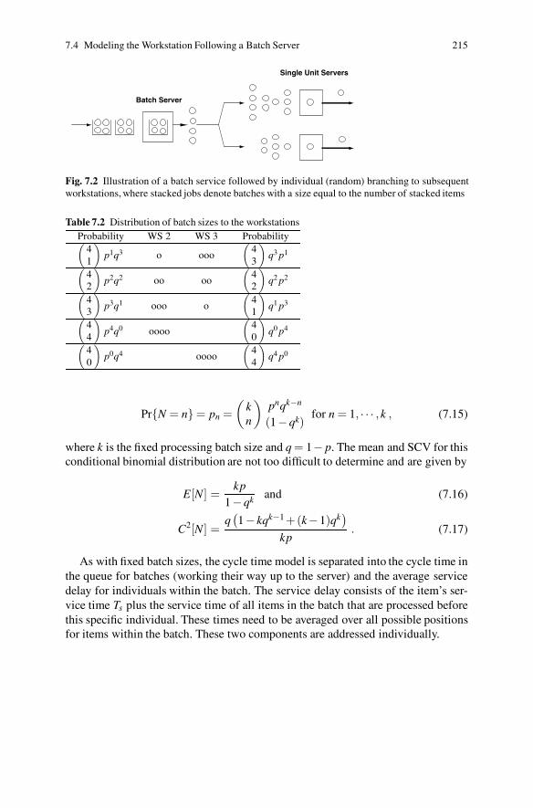
7.4 Modeling the Workstation Following a Batch Server 215
Batch Server
Single Unit Servers
Fig. 7.2 Illustration of a batch service followed by individual (random) branching to subsequentworkstations, where stacked jobs denote batches with a size equal to the number of stacked items
Table 7.2 Distribution of batch sizes to the workstationsProbability WS 2 WS 3 Probability(
41
)
p1q3 o ooo(
43
)
q3 p1
(
42
)
p2q2 oo oo
(
42
)
q2 p2
(
43
)
p3q1 ooo o
(
41
)
q1 p3
(
44
)
p4q0 oooo
(
40
)
q0 p4
(
40
)
p0q4 oooo(
44
)
q4 p0
Pr{N = n}= pn =(
kn
)
pnqk−n
(1−qk)for n = 1, · · · ,k , (7.15)
where k is the fixed processing batch size and q = 1− p. The mean and SCV for thisconditional binomial distribution are not too difficult to determine and are given by
E[N] =kp
1−qk and (7.16)
C2[N] =q(
1− kqk−1 +(k−1)qk)
kp. (7.17)
As with fixed batch sizes, the cycle time model is separated into the cycle time inthe queue for batches (working their way up to the server) and the average servicedelay for individuals within the batch. The service delay consists of the item’s ser-vice time Ts plus the service time of all items in the batch that are processed beforethis specific individual. These times need to be averaged over all possible positionsfor items within the batch. These two components are addressed individually.
216 7 Models of Various Forms of Batching
7.4.2.1 Cycle Time in the Queue for Random Sized Batches
A queued batch can be viewed as seeing batches ahead of it being served as a wholeeven though the service mechanism operates on individual items taken from a batch.The expected delay time is computed for a batch to move up in the first-come-first-serve queue until it (any of its items) becomes the batch being served. (This is thesame model form used for the Batch Move Model of Sect. 7.1). The service timefor each batch is a random sum of i.i.d. random variables which was describedin Sect. 1.6.2. Thus, the measures for the batch service time are obtained throughProperty 1.9 and are given as
E[Ts(B)] = E[N]E[Ts(I)] and
C2[Ts(B)] = C2[N]+C2[Ts(I)]
E[N], (7.18)
where N is the random variable denoting the batch size (Eq. 7.15).The arrival rate of individual items at the workstation following a batch service
with branching probability p is a function of the arrival rate of individuals intothe batch service workstation. For notational clarification denote the batch serverworkstation as #1 and the recipient workstation as #2. Let λ1(I) be the arrival rate ofindividuals into the batch workstation and let λ2(I) be the arrival rate of individualsinto #2 after the branch. Then the relationship between these rates is
λ2(I) = pλ1(I) . (7.19)
However, the batch arrival rate is not quite as straight forward because of the pos-sibility that a batch is of size zero. Assume that #1 operates on batches of size k,then the probability that a batch of size zero is “sent” to #2 is qk where q = 1− p.Therefore, the probability that a batch of size greater than zero departs from #1 is1−qk so that the batch arrival rate to #2 is given by
λ2(B) =(
1−qk) λ1(I)
k, (7.20)
and the expected batch size is given by Eq. (7.16).The squared coefficient of variation of the inter-arrival time into #2 is related
to the squared coefficient of variation of the inter-departure time for #1. Since thedepartures are in terms of batches, the batch inter-arrival time’s squared coefficientof variation into #2 is
C2B[Ta(2)] = (1−qk)C2
B[Td(1)]+qk , (7.21)
where the subscript B is used to indicate that the C2 is for batches. Recall that thefactor qk is the probability that no units from the batch are directed to #2.
Using the standard Kingman approximation, the cycle time in the queue, CTq, forthe batches is given as
7.4 Modeling the Workstation Following a Batch Server 217
CTq(2) =(
C2B[Ta(2)]+C2[Ts(B)]
2
)(
u2
1−u2
)
E[Ts(B)] (7.22)
=(
C2B[Ta(2)]+C2[N]+C2[Ts(I)]/E[N]
2
)(
u2
1−u2
)
E[N]E[Ts(I)] ,
where the utilization factor is computed by u2 = λ2(I)E[Ts(I)].
• Suggestion: Do Problem 7.13.
7.4.2.2 Average Service Delay Times for Random Sized Batches
Once a batch has worked its way through the batch queue and finally has commandof the server, the server will be busy for the specific number of service times equalto the number of items in the batch. The delay time associated with individual itemswithin the batch varies since processed items leave the workstation immediatelyupon completion of their turn in the server. Thus, an average delay is computed bytaking into account the delay associated with each position, with respect to the orderthat items are served, within the batch. This average delay has two components,the service time of the individual and the average delay waiting for other itemspositioned ahead of that individual unit in the batch.
We follow the same logic here that was used in Sect. 7.1.3. The random vari-able D represents the total delay experienced by all jobs within a batch; thus fromEq. (7.5), it follows that
E[D|N = n] =n(n−1)
2E[Ts(I)] ,
where the random variable N is the size of the batch. Since E[E[D|N] ]= E[D] (seeProperty 1.8), the service time delay, st , is obtained as follows
st =E[D]E[N]
+E[Ts(I)] =E[N(N−1)]
2E[N]E[Ts(I)]+E[Ts(I)] (7.23)
=E[N(N +1)]
2E[N]E[Ts(I)] =
E[N2]−E[N]2 +E[N]2 +E[N]2E[N]
E[Ts(I)]
=(
E[N]+12
+V [N]2E[N]
)
E[Ts(I)] =(
1 +E[N]+E[N]C2[N]2
)
E[Ts(I)] .
Notice that for deterministic batches, Eq. (7.23) is identical to Eq. (7.6).

218 7 Models of Various Forms of Batching
7.4.2.3 Cycle Time in the Workstation for Random Sized Batches
The cycle time in a workstation that directly follows a batch server and receivesonly a proportion of the individual items can be obtained by combining the twomajor pieces of the previous two sections yielding the following property.
Property 7.8. Consider a workstation that processes items one-at-a-time witha mean and SCV of the (individual) processing time given by E[Ts] and C2
s .Jobs arrive to the workstation in batches of random size denoted by N. Thetimes between batch arrivals have a mean and SCV of E[Ta(B)] and C2
B[Ta]yielding a mean batch arrival rate of λ (B) = 1/E[Ta(B)]. The mean systemcycle time per item at the workstation is approximated by
CTs =(
E[N]C2B[Ta]+E[N]C2[N]+C2
s
2
)(
u1−u
)
E[Ts]
+(
1 +E[N]+E[N]C2[N]2
)
E[Ts]
where the utilization factor is u = E[N]λ (B)E[Ts].
Example 7.4. Consider a workstation that processes 5 units simultaneously (k = 5).Let the departure rate from this batch workstation be 3 batches per hour with asquared coefficient of variation of the inter-departure times of 0.75. After the batchleaves the workstation, it is broken into individual units and each item has a 25%chance of being sent to the second workstation. The second workstation processesitems one-at-a-time according to an exponential distribution with mean of 12 min-utes. We would like to analyze the second workstation.
The probability of #2 not receiving any units from a particular batch that finishedprocessing at #1 is 0.755 = 0.2373. Thus, the arrival rate of of batches (of any size)to #2 is λa(B) = 3(1− 0.2373) = 2.288 per hour (see Eq. 7.20), or equivalently,E[Ta(B)] = 0.437 hours. Note that the arriving batch can be of any size from 1 to5 units depending on the probabilistic results from individual unit branching. Themean and SCV for the batch size (Eqs. 7.16 and 7.17) are E[N]= 1.639 and C2[N]=0.220. The mean batch size (1.639) together with the batch arrival rate (2.288/hr)and the mean service time (0.2 hr) results in a utilization factor of u = 0.75.
The arrival rate of individual units is the average batch size (1.639) times thebatch arrival rate (2.288/hr) yielding 3.75/hr which is also equal to the branch prob-ability (0.25) times the individual departure rate from the first workstation. TheSCV of the inter-arrival times of batches is determined from the departure processaccording to Eq. (7.21):
C2B[Ta] = (1−0.2373)0.75+0.2373 = 0.809.
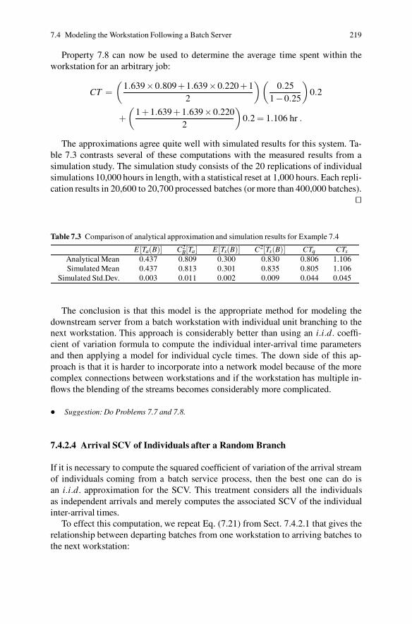
7.4 Modeling the Workstation Following a Batch Server 219
Property 7.8 can now be used to determine the average time spent within theworkstation for an arbitrary job:
CT =(
1.639×0.809+1.639×0.220 +12
)(
0.251−0.25
)
0.2
+(
1 +1.639 +1.639×0.2202
)
0.2 = 1.106 hr .
The approximations agree quite well with simulated results for this system. Ta-ble 7.3 contrasts several of these computations with the measured results from asimulation study. The simulation study consists of the 20 replications of individualsimulations 10,000 hours in length, with a statistical reset at 1,000 hours. Each repli-cation results in 20,600 to 20,700 processed batches (or more than 400,000 batches).
��
Table 7.3 Comparison of analytical approximation and simulation results for Example 7.4
E [Ta(B)] C2B[Ta] E [Ts(B)] C2[Ts(B)] CTq CTs
Analytical Mean 0.437 0.809 0.300 0.830 0.806 1.106Simulated Mean 0.437 0.813 0.301 0.835 0.805 1.106
Simulated Std.Dev. 0.003 0.011 0.002 0.009 0.044 0.045
The conclusion is that this model is the appropriate method for modeling thedownstream server from a batch workstation with individual unit branching to thenext workstation. This approach is considerably better than using an i.i.d. coeffi-cient of variation formula to compute the individual inter-arrival time parametersand then applying a model for individual cycle times. The down side of this ap-proach is that it is harder to incorporate into a network model because of the morecomplex connections between workstations and if the workstation has multiple in-flows the blending of the streams becomes considerably more complicated.
• Suggestion: Do Problems 7.7 and 7.8.
7.4.2.4 Arrival SCV of Individuals after a Random Branch
If it is necessary to compute the squared coefficient of variation of the arrival streamof individuals coming from a batch service process, then the best one can do isan i.i.d. approximation for the SCV. This treatment considers all the individualsas independent arrivals and merely computes the associated SCV of the individualinter-arrival times.
To effect this computation, we repeat Eq. (7.21) from Sect. 7.4.2.1 that gives therelationship between departing batches from one workstation to arriving batches tothe next workstation:
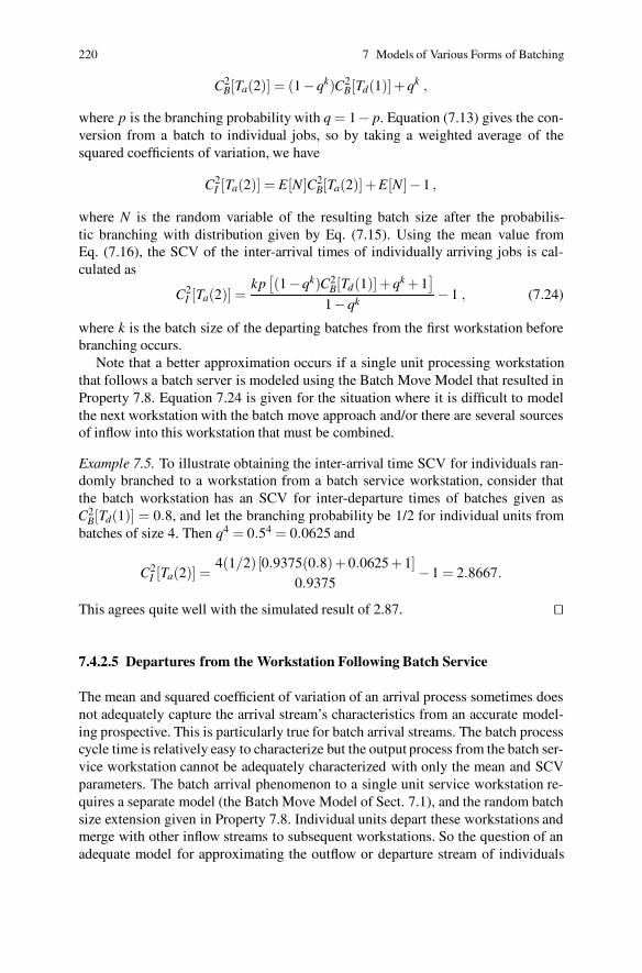
220 7 Models of Various Forms of Batching
C2B[Ta(2)] = (1−qk)C2
B[Td(1)]+qk ,
where p is the branching probability with q = 1− p. Equation (7.13) gives the con-version from a batch to individual jobs, so by taking a weighted average of thesquared coefficients of variation, we have
C2I [Ta(2)] = E[N]C2
B[Ta(2)]+E[N]−1 ,
where N is the random variable of the resulting batch size after the probabilis-tic branching with distribution given by Eq. (7.15). Using the mean value fromEq. (7.16), the SCV of the inter-arrival times of individually arriving jobs is cal-culated as
C2I [Ta(2)] =
kp[
(1−qk)C2B[Td(1)]+qk +1
]
1−qk −1 , (7.24)
where k is the batch size of the departing batches from the first workstation beforebranching occurs.
Note that a better approximation occurs if a single unit processing workstationthat follows a batch server is modeled using the Batch Move Model that resulted inProperty 7.8. Equation 7.24 is given for the situation where it is difficult to modelthe next workstation with the batch move approach and/or there are several sourcesof inflow into this workstation that must be combined.
Example 7.5. To illustrate obtaining the inter-arrival time SCV for individuals ran-domly branched to a workstation from a batch service workstation, consider thatthe batch workstation has an SCV for inter-departure times of batches given asC2
B[Td(1)] = 0.8, and let the branching probability be 1/2 for individual units frombatches of size 4. Then q4 = 0.54 = 0.0625 and
C2I [Ta(2)] =
4(1/2) [0.9375(0.8)+0.0625 +1]0.9375
−1 = 2.8667.
This agrees quite well with the simulated result of 2.87. ��
7.4.2.5 Departures from the Workstation Following Batch Service
The mean and squared coefficient of variation of an arrival process sometimes doesnot adequately capture the arrival stream’s characteristics from an accurate model-ing prospective. This is particularly true for batch arrival streams. The batch processcycle time is relatively easy to characterize but the output process from the batch ser-vice workstation cannot be adequately characterized with only the mean and SCVparameters. The batch arrival phenomenon to a single unit service workstation re-quires a separate model (the Batch Move Model of Sect. 7.1), and the random batchsize extension given in Property 7.8. Individual units depart these workstations andmerge with other inflow streams to subsequent workstations. So the question of anadequate model for approximating the outflow or departure stream of individuals
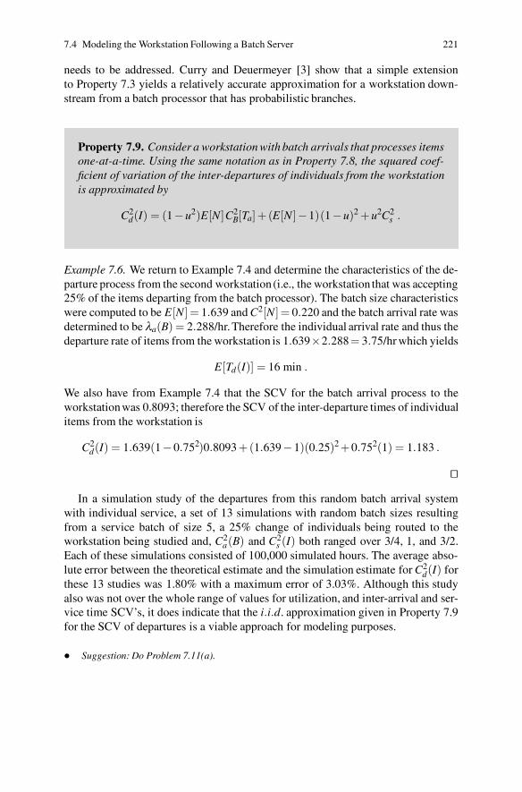
7.4 Modeling the Workstation Following a Batch Server 221
needs to be addressed. Curry and Deuermeyer [3] show that a simple extensionto Property 7.3 yields a relatively accurate approximation for a workstation down-stream from a batch processor that has probabilistic branches.
Property 7.9. Consider a workstation with batch arrivals that processes itemsone-at-a-time. Using the same notation as in Property 7.8, the squared coef-ficient of variation of the inter-departures of individuals from the workstationis approximated by
C2d(I) = (1−u2)E[N]C2
B[Ta]+ (E[N]−1)(1−u)2 +u2C2s .
Example 7.6. We return to Example 7.4 and determine the characteristics of the de-parture process from the second workstation (i.e., the workstation that was accepting25% of the items departing from the batch processor). The batch size characteristicswere computed to be E[N]= 1.639 and C2[N]= 0.220 and the batch arrival rate wasdetermined to be λa(B) = 2.288/hr. Therefore the individual arrival rate and thus thedeparture rate of items from the workstation is 1.639×2.288= 3.75/hr which yields
E[Td(I)] = 16 min .
We also have from Example 7.4 that the SCV for the batch arrival process to theworkstation was 0.8093; therefore the SCV of the inter-departure times of individualitems from the workstation is
C2d(I) = 1.639(1−0.752)0.8093 +(1.639−1)(0.25)2 +0.752(1) = 1.183 .
��
In a simulation study of the departures from this random batch arrival systemwith individual service, a set of 13 simulations with random batch sizes resultingfrom a service batch of size 5, a 25% change of individuals being routed to theworkstation being studied and, C2
a(B) and C2s (I) both ranged over 3/4, 1, and 3/2.
Each of these simulations consisted of 100,000 simulated hours. The average abso-lute error between the theoretical estimate and the simulation estimate for C2
d(I) forthese 13 studies was 1.80% with a maximum error of 3.03%. Although this studyalso was not over the whole range of values for utilization, and inter-arrival and ser-vice time SCV’s, it does indicate that the i.i.d. approximation given in Property 7.9for the SCV of departures is a viable approach for modeling purposes.
• Suggestion: Do Problem 7.11(a).

222 7 Models of Various Forms of Batching
7.5 Batch Network Examples
Modeling the flow of jobs within a factory in which batching occurs can compli-cate the methodology considerably. To help in incorporating batches within yourmodels, we devote this final section to the analysis of two different factories withbatching. The first example includes all three major batch types and without anyfeedback paths. The second example includes a more complex branching structurethat has reentrant flows. The main concept that is demonstrated with these examplesis that the formulas from the various properties cannot be blindly applied — theyoften must be adjusted slightly to fit different situations. However, the bottom lineis that systems with batching can be reasonably well analyzed if the various modelsdiscussed in this chapter are used wisely.
7.5.1 Batch Network Example 1
Consider Fig. 7.3 that has three workstations each of which operates using a differ-ent form of the batch service models studied in this chapter. The first workstation isa setup-batch processing workstation, the second workstation uses oven-batch pro-cessing, and the third workstation is a single unit server with batch arrivals (thebatch move model). Inflow into the system is in terms of individual units with aPoisson arrival rate with a mean of 5 units per hour. These individuals are imme-diately batched into groups of k = 3 and transported into the first workstation. Thebatch forming time in this analysis will be added to the cycle time for Workstation1. The data for each particular workstation is given as it is needed in the solutionprocess.
Note in Fig. 7.3 that once batches are formed, they remain batches until they ei-ther exit the system following processing at Workstation 2 or they make it to Work-station 3. The jobs are large and require a forklift for transportation between work-stations, thus all probabilistic branches are made on batches and not individual jobs.Specifically, 2/3 of the batches leaving Workstation 1 are routed to Workstation 2and 1/3 go to Workstation 3. From Workstation 2, 1/4 of the batches are finished(leave the system) and the remaining 3/4 are routed to Workstation 3. At Worksta-tion 3, the items are then separated once the batch enters service and, subsequently,they leave as individuals. The goal of this analysis is to obtain the expected cycletime and throughput rate for the system as a whole.
Workstation 1 Including Batch Forming Time
The arrival rate of individuals to the first workstation is according to a Poisson pro-cess with a mean rate of 5 per hour. The average batch forming time, BT , to beassociated with each individual item is determined by the equation

7.5 Batch Network Examples 223
q
1-q
p
1-p
Batch Form
Size = k
Setup Batch
Oven Batch
Single Item
Fig. 7.3 Example manufacturing system where each workstation in the facility uses a differentform of the batch processing models
BTstart =(3−1)
215
= 0.2 hr ,
where the 1/5 hour is the mean inter-arrival time. The arrival rate of batches to Work-station 1 is the individual arrival rate divided by the batch size yielding λ1(B) = 5/3per hour. Since the external arrival process is Poisson, the squared coefficient ofvariation of the arrival stream of individuals is 1. Thus, the SCV for the inter-arrivaltime of batches is
C2B[Ta(1)] =
13
.
The first workstation is a setup batch system where a setup is required for everythree jobs. The setup time has a mean of 12 minutes and a variance of 1080 minutes2.After the setup, jobs are processed one-at-a-time with a mean processing time of 6minutes and a variance of 240 minutes2. Thus the characteristics for processing theentire batch is given as
E[Ts,1(B)] = 12 +3×6 = 30 min = 0.5 hr
V [Ts,1(B)] = 1080 +3×240 = 1800 min2 = 0.5 hr2
C2s,1(B) =
0.50.52 = 2 .
The workstation utilization is u1 = λ1(B)× E[Ts,1(B)] = 0.8333.Before usingProperty 7.4 to determine the average cycle time within the first workstation, weneed to add a batch forming time after processing. Because all jobs are moved be-tween workstations by a batch move, we add the batch forming time to the endof this cycle time. (Although the formula of Property 7.1 includes the batch form-
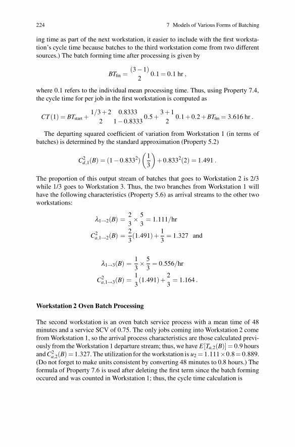
224 7 Models of Various Forms of Batching
ing time as part of the next workstation, it easier to include with the first worksta-tion’s cycle time because batches to the third workstation come from two differentsources.) The batch forming time after processing is given by
BTfin =(3−1)
20.1 = 0.1 hr ,
where 0.1 refers to the individual mean processing time. Thus, using Property 7.4,the cycle time for per job in the first workstation is computed as
CT (1) = BTstart +1/3 +2
20.8333
1−0.83330.5 +
3 +12
0.1 +0.2 +BTfin = 3.616 hr .
The departing squared coefficient of variation from Workstation 1 (in terms ofbatches) is determined by the standard approximation (Property 5.2)
C2d,1(B) = (1−0.8332)
(
13
)
+0.8332(2) = 1.491 .
The proportion of this output stream of batches that goes to Workstation 2 is 2/3while 1/3 goes to Workstation 3. Thus, the two branches from Workstation 1 willhave the following characteristics (Property 5.6) as arrival streams to the other twoworkstations:
λ1→2(B) =23× 5
3= 1.111/hr
C2a,1→2(B) =
23(1.491)+
13
= 1.327 and
λ1→3(B) =13× 5
3= 0.556/hr
C2a,1→3(B) =
13(1.491)+
23
= 1.164 .
Workstation 2 Oven Batch Processing
The second workstation is an oven batch service process with a mean time of 48minutes and a service SCV of 0.75. The only jobs coming into Workstation 2 comefrom Workstation 1, so the arrival process characteristics are those calculated previ-ously from the Workstation 1 departure stream; thus, we have E[Ta,2(B)] = 0.9 hoursand C2
a,2(B) = 1.327. The utilization for the workstation is u2 = 1.111×0.8= 0.889.(Do not forget to make units consistent by converting 48 minutes to 0.8 hours.) Theformula of Property 7.6 is used after deleting the first term since the batch formingoccured and was counted in Workstation 1; thus, the cycle time calculation is
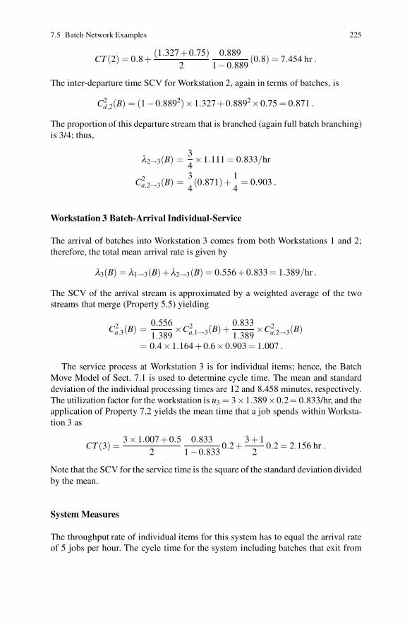
7.5 Batch Network Examples 225
CT (2) = 0.8 +(1.327 +0.75)
20.889
1−0.889(0.8) = 7.454 hr .
The inter-departure time SCV for Workstation 2, again in terms of batches, is
C2d,2(B) = (1−0.8892)×1.327 +0.8892×0.75 = 0.871 .
The proportion of this departure stream that is branched (again full batch branching)is 3/4; thus,
λ2→3(B) =34×1.111 = 0.833/hr
C2a,2→3(B) =
34(0.871)+
14
= 0.903 .
Workstation 3 Batch-Arrival Individual-Service
The arrival of batches into Workstation 3 comes from both Workstations 1 and 2;therefore, the total mean arrival rate is given by
λ3(B) = λ1→3(B)+λ2→3(B) = 0.556 +0.833 = 1.389/hr .
The SCV of the arrival stream is approximated by a weighted average of the twostreams that merge (Property 5.5) yielding
C2a,3(B) =
0.5561.389
×C2a,1→3(B)+
0.8331.389
×C2a,2→3(B)
= 0.4×1.164 +0.6×0.903 = 1.007 .
The service process at Workstation 3 is for individual items; hence, the BatchMove Model of Sect. 7.1 is used to determine cycle time. The mean and standarddeviation of the individual processing times are 12 and 8.458 minutes, respectively.The utilization factor for the workstation is u3 = 3×1.389×0.2= 0.833/hr, and theapplication of Property 7.2 yields the mean time that a job spends within Worksta-tion 3 as
CT (3) =3×1.007 +0.5
20.833
1−0.8330.2 +
3 +12
0.2 = 2.156 hr .
Note that the SCV for the service time is the square of the standard deviation dividedby the mean.
System Measures
The throughput rate of individual items for this system has to equal the arrival rateof 5 jobs per hour. The cycle time for the system including batches that exit from

226 7 Models of Various Forms of Batching
Workstation 2 is determined by computing the work-in-process (W IP) at each work-station, then summing to obtain the system W IP. From the system W IP, using Lit-tle’s Law (WIP = th×CT ), the cycle time for individuals is determined. Note thatthe W IP is to be computed in individual units so that the cycle time for individualsin the system can be computed. The data needed for this analysis and the results arecontained in Table 7.4.
Table 7.4 W IP calculations for the example of Sect. 7.5.1
Workstation i λi(I) CT(i) W IP(i)1 5/hr 3.616 hr 18.082 3.333/hr 7.454 hr 24.843 4.167/hr 2.156 hr 8.98
Table 7.5 Transportation time calculations for the example of Sect. 7.5.1
From/To Move Rate Travel Time W IPEntrance to WS 1 5/hr 5 min 0.417
WS 1 to WS 2 3.333/hr 8 min 0.444WS 1 to WS 3 1.668/hr 9 min 0.250WS 2 to WS 3 2.499/hr 6 min 0.250
Thus, the total system W IP is 51.9 jobs and the average cycle time for individualjobs through this system regardless of their exit point is 51.9/5 = 10.38 hours. Thesecalculations ignored all transportation times. If we assume a sufficient number offorklifts so that there is no waiting when a batch is ready to be moved, it is relativelyeasy to include the time necessary for batch moves. Table 7.5 shows the data andthe calculations needed to include the transportation time needed for the forklifts tomove the various jobs between workstations.
From the analysis contained in Table 7.5, we have that there is an average of1.36 jobs within the transportation system of the factory. Thus, the total W IP in thefactory is 53.26 jobs and the mean cycle time, including move times, is 10.65 hours.
7.5.2 Batch Network Example 2
Consider the network given in Fig. 7.4. The first workstation has two processingmachines, the second workstation has one machine, and the third workstation hasan oven process that serves three units simultaneously. The arrival rate of jobs intothis system is a Poisson process with jobs entering at Workstation 1 at a mean rateof 10 jobs per hour. The data for the three workstations are given in Table 7.6.
Because there are reentrant flows within this factory, the total arrivals rates mustbe determined using a routing matrix. These probabilities given in Fig. 7.4 and result
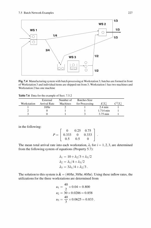
7.5 Batch Network Examples 227
WS 3
WS 1
WS 2
1/4
3/4
1/2
1/2
1/3
1/3
1/3
Fig. 7.4 Manufacturingsystem with batch processingat Workstation 3; batches are formed in frontof Workstation 3 and individual items are shipped out from 3; Workstation 1 has two machines andWorkstation 2 has one machine
Table 7.6 Data for the example of Sect. 7.5.2
External Number of Batches SizeWorkstation Arrival Rate Machines for Processing E [Ts] C2[Ts]
1 10/hr 2 1 2.4 min 12 0 1 1 1.714 min 13 0 1 3 3.75 min 1
in the following:
P =
⎡
⎣
0 0.25 0.750.333 0 0.333
0.5 0.5 0
⎤
⎦ .
The mean total arrival rate into each workstation, λi for i = 1,2,3, are determinedfrom the following system of equations (Property 5.7):
λ1 = 10 +λ2/3 +λ3/2
λ2 = λ1/4 +λ3/2
λ3 = 3λ1/4 +λ2/3 .
The solution to this system is λλλ = (40/hr,30/hr,40/hr). Using these inflow rates, theutilizations for the three workstations are determined from
u1 =402
×0.04 = 0.800
u2 = 30×0.0286 = 0.858
u3 =403
×0.0625 = 0.833 .
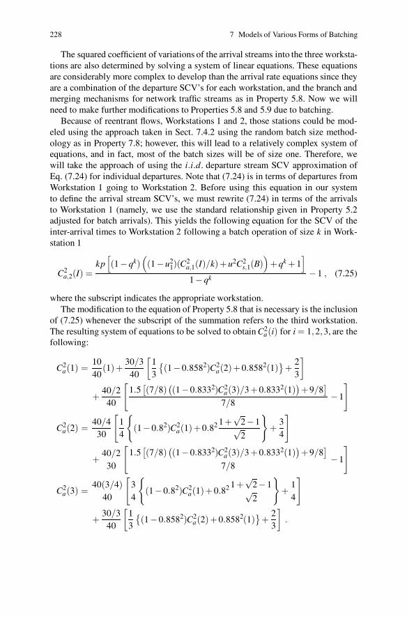
228 7 Models of Various Forms of Batching
The squared coefficient of variations of the arrival streams into the three worksta-tions are also determined by solving a system of linear equations. These equationsare considerably more complex to develop than the arrival rate equations since theyare a combination of the departure SCV’s for each workstation, and the branch andmerging mechanisms for network traffic streams as in Property 5.8. Now we willneed to make further modifications to Properties 5.8 and 5.9 due to batching.
Because of reentrant flows, Workstations 1 and 2, those stations could be mod-eled using the approach taken in Sect. 7.4.2 using the random batch size method-ology as in Property 7.8; however, this will lead to a relatively complex system ofequations, and in fact, most of the batch sizes will be of size one. Therefore, wewill take the approach of using the i.i.d. departure stream SCV approximation ofEq. (7.24) for individual departures. Note that (7.24) is in terms of departures fromWorkstation 1 going to Workstation 2. Before using this equation in our systemto define the arrival stream SCV’s, we must rewrite (7.24) in terms of the arrivalsto Workstation 1 (namely, we use the standard relationship given in Property 5.2adjusted for batch arrivals). This yields the following equation for the SCV of theinter-arrival times to Workstation 2 following a batch operation of size k in Work-station 1
C2a,2(I) =
kp[
(1−qk)(
(1−u21)(C
2a,1(I)/k)+u2C2
s,1(B))
+qk +1]
1−qk−1 , (7.25)
where the subscript indicates the appropriate workstation.The modification to the equation of Property 5.8 that is necessary is the inclusion
of (7.25) whenever the subscript of the summation refers to the third workstation.The resulting system of equations to be solved to obtain C2
a(i) for i = 1,2,3, are thefollowing:
C2a(1) =
1040
(1)+30/3
40
[
13
{
(1−0.8582)C2a(2)+0.8582(1)
}
+23
]
+40/2
40
[
1.5[
(7/8)(
(1−0.8332)C2a(3)/3 +0.8332(1)
)
+9/8]
7/8−1
]
C2a(2) =
40/430
[
14
{
(1−0.82)C2a(1)+0.82 1 +
√2−1√2
}
+34
]
+40/2
30
[
1.5[
(7/8)(
(1−0.8332)C2a(3)/3 +0.8332(1)
)
+9/8]
7/8−1
]
C2a(3) =
40(3/4)40
[
34
{
(1−0.82)C2a(1)+0.82 1 +
√2−1√2
}
+14
]
+30/3
40
[
13
{
(1−0.8582)C2a(2)+0.8582(1)
}
+23
]
.
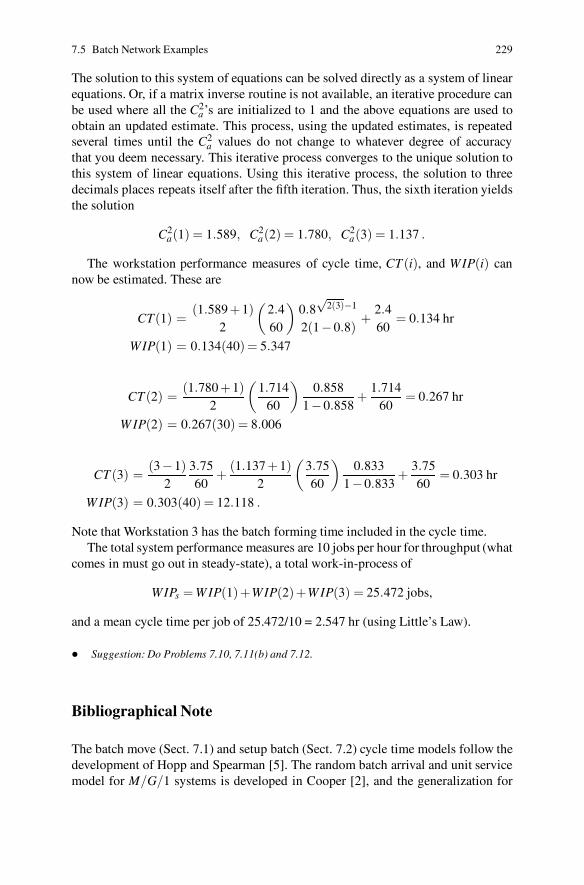
7.5 Batch Network Examples 229
The solution to this system of equations can be solved directly as a system of linearequations. Or, if a matrix inverse routine is not available, an iterative procedure canbe used where all the C2
a’s are initialized to 1 and the above equations are used toobtain an updated estimate. This process, using the updated estimates, is repeatedseveral times until the C2
a values do not change to whatever degree of accuracythat you deem necessary. This iterative process converges to the unique solution tothis system of linear equations. Using this iterative process, the solution to threedecimals places repeats itself after the fifth iteration. Thus, the sixth iteration yieldsthe solution
C2a(1) = 1.589, C2
a(2) = 1.780, C2a(3) = 1.137 .
The workstation performance measures of cycle time, CT (i), and WIP(i) cannow be estimated. These are
CT(1) =(1.589 +1)
2
(
2.460
)
0.8√
2(3)−1
2(1−0.8)+
2.460
= 0.134 hr
WIP(1) = 0.134(40)= 5.347
CT (2) =(1.780 +1)
2
(
1.71460
)
0.8581−0.858
+1.714
60= 0.267 hr
W IP(2) = 0.267(30) = 8.006
CT (3) =(3−1)
23.7560
+(1.137 +1)
2
(
3.7560
)
0.8331−0.833
+3.7560
= 0.303 hr
W IP(3) = 0.303(40) = 12.118 .
Note that Workstation 3 has the batch forming time included in the cycle time.The total system performance measures are 10 jobs per hour for throughput (what
comes in must go out in steady-state), a total work-in-process of
WIPs = W IP(1)+WIP(2)+W IP(3) = 25.472 jobs,
and a mean cycle time per job of 25.472/10 = 2.547 hr (using Little’s Law).
• Suggestion: Do Problems 7.10, 7.11(b) and 7.12.
Bibliographical Note
The batch move (Sect. 7.1) and setup batch (Sect. 7.2) cycle time models follow thedevelopment of Hopp and Spearman [5]. The random batch arrival and unit servicemodel for M/G/1 systems is developed in Cooper [2], and the generalization for

230 7 Models of Various Forms of Batching
the G/G/1 case developed herein agrees with his result for Poisson arrivals. Therenewal process approximations for the departure SCV’s from the various batchservice processes are developed in Curry and Deuermeyer [3]. The developmentapproach is an extension of the G/G/1 departure process analysis of Buzacott andShanthikumar [6]. A more general batching rule is contained in [4] where insteadof using a fixed batch size, a minimum size and a maximum size are establishedso that processing would begin whenever the minimum size is available but if morethat the maximum number of items are queued at the end of an operation, only themaximum would be allowed in the processor.
Problems
7.1. Consider a system with a single workstation that processes jobs one at a time.Jobs arrive to the factory at a rate of one per hour. An analysis of the arrival dataindicates that these inter-arrival times have a squared coefficient of variation (SCV)of 1.5. The service time mean is 0.75 hours with an SCV of 2. The company policy isto work on orders k at a time. That is, orders are held until there are k jobs, then thisgroup of jobs is released into the factory for processing. Since there is no physicalreason for holding the incoming work and forcing it into groups, what is the impacton cycle time of this ”batching” operation for specified k values?(a) k = 2.(b) k = 3.(c) k = 4.(d) k = 5.
7.2. Consider a factory that has a single workstation that processes parts individu-ally. These parts are quite heavy and the company policy is to palatalize incomingparts into groups of k items for ease of transportation. These batches are then re-leased into the factory for processing. These k items are processed at the machineand again placed back on the pallet. When the pallet is full, the k items have beenprocessed, the pallet is transported to shipping.(a) Neglecting the actual transportation time, what is the equation for cycle time ofindividual parts for this factory. This cycle time includes the waiting time for allbatching operations. Compare the batch movement cycle time with that of a systemthat does not need to batch these items for movement within the factory. How muchextra time does an average item incur due to batching for movement purposes?(b) Assume it takes an average of t1 to move a pallet from the unloading dock to theworkstation and an average of t2 to move a pallet from the machine to the next work-station. Assuming no waiting for a forklift to move the pallet, add the transportationtime to the model.
7.3. Consider a factory that processes a single job type. Orders are processed one ata time in a serial processing configuration. One of the workstations requires a ma-chine cleaning operation periodically. This workstation has only one machine. No
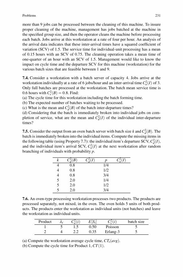
Problems 231
more than 9 jobs can be processed between the cleaning of this machine. To insureproper cleaning of the machine, management has jobs batched at the machine inthe specified group size, and then the operator cleans the machine before processingeach batch. Jobs arrive at this workstation at a rate of four per hour. An analysis ofthe arrival data indicates that these inter-arrival times have a squared coefficient ofvariation (SCV) of 1.5. The service time for individual-unit processing has a meanof 0.15 hours with an SCV of 0.75. The cleaning operation takes a mean time ofone-quarter of an hour with an SCV of 1.5. Management would like to know theimpact on cycle time and the departure SCV for this machine (workstation) for thevarious batch sizes that are feasible between 1 and 9.
7.4. Consider a workstation with a batch server of capacity 4. Jobs arrive at theworkstation individually at a rate of 6 jobs/hour and an inter-arrival time C2
a(I) of 3.Only full batches are processed at the workstation. The batch mean service time is0.6 hours with C2
s (B) = 0.8. Find:(a) The cycle time for this workstation including the batch forming time.(b) The expected number of batches waiting to be processed.(c) What is the mean and C2
d(B) of the batch inter-departure times?(d) Considering that the batch is immediately broken into individual jobs on com-pletion of service, what are the mean and C2
d(I) of the individual inter-departuretimes?
7.5. Consider the output from an oven batch server with batch size k and C2d(B). The
batch is immediately broken into the individual items. Compute the missing items inthe following table (using Property 7.7): the individual item’s departure SCV, C2
d(I),and the individual item’s arrival SCV, C2
a(I) at the next workstation after randombranching of individuals with probability p.
k C2d(B) C2
d(I) p C2a(I)
4 0.8 1/44 0.8 1/24 0.8 3/45 2.0 1/45 2.0 1/25 2.0 3/4
7.6. An oven-type processing workstation processes two products. The products areprocessed separately, not mixed, in the oven. The oven holds 5 units of both prod-ucts. The products enter the workstation as individual units (not batches) and leavethe workstation as individual units.
Product λi C2a(i) E[Si] C2
s (i) batch size1 5 1.5 0.50 Poisson 52 4 2.2 0.35 Erlang-3 5
(a) Compute the workstation average cycle time, CTs(avg).(b) Compute the cycle time for Product 1, CT (1).
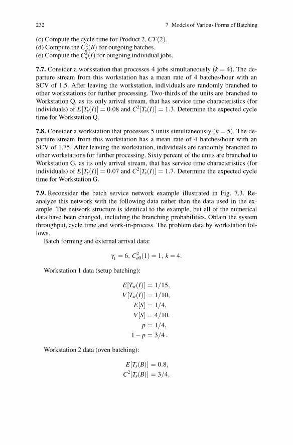
232 7 Models of Various Forms of Batching
(c) Compute the cycle time for Product 2, CT (2).(d) Compute the C2
d(B) for outgoing batches.(e) Compute the C2
d(I) for outgoing individual jobs.
7.7. Consider a workstation that processes 4 jobs simultaneously (k = 4). The de-parture stream from this workstation has a mean rate of 4 batches/hour with anSCV of 1.5. After leaving the workstation, individuals are randomly branched toother workstations for further processing. Two-thirds of the units are branched toWorkstation Q, as its only arrival stream, that has service time characteristics (forindividuals) of E[Ts(I)] = 0.08 and C2[Ts(I)] = 1.3. Determine the expected cycletime for Workstation Q.
7.8. Consider a workstation that processes 5 units simultaneously (k = 5). The de-parture stream from this workstation has a mean rate of 4 batches/hour with anSCV of 1.75. After leaving the workstation, individuals are randomly branched toother workstations for further processing. Sixty percent of the units are branched toWorkstation G, as its only arrival stream, that has service time characteristics (forindividuals) of E[Ts(I)] = 0.07 and C2[Ts(I)] = 1.7. Determine the expected cycletime for Workstation G.
7.9. Reconsider the batch service network example illustrated in Fig. 7.3. Re-analyze this network with the following data rather than the data used in the ex-ample. The network structure is identical to the example, but all of the numericaldata have been changed, including the branching probabilities. Obtain the systemthroughput, cycle time and work-in-process. The problem data by workstation fol-lows.
Batch forming and external arrival data:
γ1 = 6, C2a0(1) = 1, k = 4.
Workstation 1 data (setup batching):
E[Tsi(I)] = 1/15,
V [Tsi(I)] = 1/10,
E[S] = 1/4,
V [S] = 4/10.
p = 1/4,
1− p = 3/4 .
Workstation 2 data (oven batching):
E[Ts(B)] = 0.8,
C2[Ts(B)] = 3/4,

Problems 233
q = 1/3,
1−q = 2/3 .
Workstation 3 (batch move):
E[Ts(I)] = 1/5,
C2[Ts(I)] = 1/2 .
7.10. Consider a factory with a batch server. Let the network structure be the sameas that of Fig. 7.4, except that the branching probabilities are different. The datafor the workstations and the branching probabilities are given below. Develop theworkstation and system performance measures of throughput, cycle time and work-in-process. The external arrival process is assumed to be Poisson. Note: use (7.25)in the C2
a(I) term.
Workstation Inflow Machines Batches E[Ts] C2[Ts]1 10 2 1 1/25 22 0 1 1 1/35 23 0 1 4 1/10 2
From/To 1 2 31 0 1/3 2/32 1/3 0 1/33 4/10 6/10 0
7.11. Consider a network of four workstations with the data given in the followingtables. Draw the network diagram and develop the workstation and system perfor-mance measures of throughput, cycle time and work-in-process. The external arrivalprocess is assumed to be Poisson.(a) Use Property 7.7 in the C2
a(I) computations.(b) Use Eq. (7.25) in the C2
a(I) computations.
Workstation Inflow Machines Batch Size E[Ts] C2[Ts]1 2.5 1 1 0.10 2.002 1 2 1 0.26 1.503 0 1 1 0.13 0.754 0 1 4 0.64 3.00
From/To 1 2 3 41 0 2/4 1/4 1/42 1/3 0 1/3 1/33 4/8 1/8 0 1/84 0 0 2/3 0
7.12. A manufacturer produces two products in a three-workstation facility. Theproducts are similar and both use an identical heat-treatment process. Thus, theseproducts can be indiscriminately mixed for this oven process, that can process six
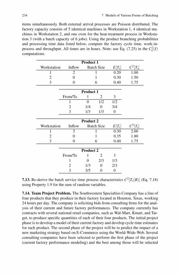
234 7 Models of Various Forms of Batching
items simultaneously. Both external arrival processes are Poisson distributed. Thefactory capacity consists of 5 identical machines in Workstation 1, 4 identical ma-chines in Workstation 2, and one oven for the heat-treatment process in Worksta-tion 3 (with a batch capacity of 6 jobs). Using the product branching probabilitiesand processing time data listed below, compute the factory cycle time, work-in-process and throughput. All times are in hours. Note: use Eq. (7.25) in the C2
a(I)computations.
Product 1Workstation Inflow Batch Size E[Ts] C2[Ts]
1 2 1 0.20 1.002 0 1 0.30 1.503 0 6 0.40 1.75
Product 1From/To 1 2 3
1 0 1/2 1/22 1/4 0 3/43 1/3 1/3 0
Product 2Workstation Inflow Batch Size E[Ts] C2[Ts]
1 3 1 0.30 2.002 0 1 0.35 1.803 0 6 0.40 1.75
Product 2From/To 1 2 3
1 0 2/3 1/32 1/3 0 2/33 3/5 0 0
7.13. Re-derive the batch service time process characteristics C2[Ts(B)] (Eq. 7.18)using Property 1.9 for the sum of random variables.
7.14. Team Project Problem. The Southwestern Specialties Company has a line offour products that they produce in their factory located in Houston, Texas, working24 hours per day. The company is soliciting bids from consulting firms for the anal-ysis of their current and future factory performances. The company currently hascontracts with several national retail companies, such as Wal-Mart, Kmart, and Tar-get, to produce specific quantities of each of their four products. The initial projectphase is to develop a model of their current factory and develop cycle time estimatesfor each product. The second phase of the project will be to predict the impact of anew marketing strategy based on E-Commerce using the World-Wide-Web. Severalconsulting companies have been selected to perform the first phase of the project(current factory performance modeling) and the best among those will be selected
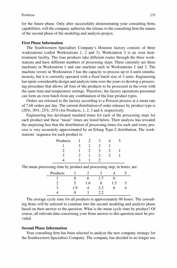
Problems 235
for the future phase. Only after successfully demonstrating your consulting firmscapabilities, will the company authorize the release to the consulting firm the natureof the second phase of the modeling and analysis project.
First Phase InformationThe Southwestern Specialties Company’s Houston factory consists of three
workstations (called Workstations 1, 2 and 3). Workstation 3 is an oven heat-treatment facility. The four products take different routes through the three work-stations and have different numbers of processing steps. There currently are threemachines in Workstation 1 and one machine each in Workstations 2 and 3. Themachine (oven) in Workstation 3 has the capacity to process up to 4 units simulta-neously, but it is currently operated with a fixed batch size of 3 units. Engineeringhas spent considerable design and analysis time over the years to develop a process-ing procedure that allows all four of the products to be processed in the oven withthe same time and temperature settings. Therefore, the factory operations personnelcan form an oven batch from any combination of the four product types.
Orders are released to the factory according to a Poisson process at a mean rateof 7.68 orders per day. The current distribution of order releases by product type is(20%, 30%, 25%, 25%) for Products, 1, 2, 3 and 4, respectively.
Engineering has developed standard times for each of the processing steps foreach product and these “mean” times are listed below. Their analysis has revealedthe surprising fact that the distribution of processing times for each and every pro-cess is very accurately approximated by an Erlang Type-2 distribution. The work-stations’ sequence for each product is:
Products 1 2 3 4 51 3 1 2 12 1 2 3 2 13 2 1 2 3 14 3 1 2
The mean processing time by product and processing step, in hours, are:
Products 1 2 3 4 51 8 6 1.7 62 5 1.6 8 1.5 53 1.9 4 2.2 8 44 8 3 2.2
The average cycle time for all products is approximately 80 hours. The consult-ing firms will be selected to continue into the second modeling and analysis phasebased on their answer to the question: What is the mean cycle time by product? Ofcourse, all relevant data concerning your firms answer to this question must be pro-vided.
Second Phase InformationYour consulting firm has been selected to analyze the new company strategy for
the Southwestern Specialties Company. The company has decided to no longer use

236 7 Models of Various Forms of Batching
Product 1
1 2 38
0.10
0.15
4 51 2 3
0.05
losses0.07
Fig. 7.5a Process flow diagram for Product 1 of Problem 7.15
1 2 34 1 2 3 5
losses
0.04
0.090.08
0.05
2
Product 2
Fig. 7.5b Process flow diagram for Product 2 of Problem 7.15
fixed contracts. They have decided that they would do better by selling the fourproducts over the internet. The research staff has determined that the sales rates arefunctions of the product cycle times and they estimate these functions as:
Product 1: r(1) = 0.1088−0.0006×CT(1),Product 2: r(2) = 0.1632−0.0007×CT(2),Product 3: r(3) = 0.1360−0.0006×CT(3),Product 4: r(4) = 0.1360−0.0009×CT(4).
The company will allow two new machines to be purchased of any type (exclud-ing ovens). The company wants answers to the following questions:(a) What should be the company capacity structure?(b) What is the projected company sales rates and cycle times for the four products?(c) Are the sales consistent and stable? If not what can be done to make them stable?(d) Is the company in a good or bad situation?
7.15. Team Project Problem. Quality Products Inc., a company that manufactureshigh-quality heat-pumps for the housing industry, has a local manufacturing facil-ity. This plant only produces heat-pumps and until recently there was only one ba-sic production process for these items. With the new environmental concerns andgovernment regulations, they have designed and recently brought into production asecond product line of heat-pumps. The production processes for the old and newproduct lines are similar, using the same equipment, but they have slightly differentprocessing sequences and processing times. The product processing sequences areillustrated in Figs. 7.5a and 7.5b. Product 1 is the old heat-pump process and Prod-uct 2 is the production sequence for the new line of heat-pumps. This first quarterof 2002 the daily releases of products to be manufactured is 8 units on the product1 and 2 units of Product 2. The average cycle time for the facility is in the neighbor-hood of 6.2 days.

Problems 237
Quality Products Inc. would like to have a consulting team perform a systemsanalysis for each quarter of the year. They expect that the total of units manufacturedto remain at a demand level of 10 per day but the product mix will change eachquarter. Their quarterly demand forecasts for daily demands by product type are:
First Quarter Second Quarter Third Quarter Fourth QuarterProduct 1 8 6 4 2Product 2 2 4 6 8
The company is concerned about their machining capacities as demands changeover time. They would also like to know what the impacts will be on their cycletimes and they want to estimate the cycle times for the individual products as wellas the facility average. If new machines are needed, they want to get these orderedand installed so that they will not suffer a short-fall in production output versusdemand.
The top-planning engineer for Quality Products Inc. has developed the data forthe old and new product processing steps. The mean processing times (in days) are:
Means Step 1 Step 2 Step 3 Step 4 Step 5 Step 6 Step 7 Step 8Product 1 0.008 0.120 0.070 0.070 0.075 0.100 0.070 0.180Product 2 0.002 0.100 0.090 0.070 0.080 0.080 0.070 0.100
SCV’s Step 1 Step 2 Step 3 Step 4 Step 5 Step 6 Step 7 Step 8Product 1 1.5 1.2 1.3 1.0 1.6 0.9 1.3 0.5Product 2 1.0 1.0 1.0 1.3 1.0 1.0 1.3 1.0
There are currently three machines in Workstation 2 and two machines at Work-station 5. The other workstations seem to be operating okay with a single processingmachine. Workstation 3 is a heat-treatment process and the current capacity of themachine is two jobs at a time.
The product demand data is currently 8 units of Product 1 per day with a SCVof 1.5. Product 2 has a mean demand rate of 2 units per day with an SCV of 0.75.As demand shifts from being predominantly Product 1 to mostly Product 2, thecompany does not anticipate a change in the SCV’s for the individual products.
All of the machines in the factory have a 95% availability factor. The mean repairtimes are, respectively, 0.2, 0.3, 0.4, 0.35, 0.5, days. All repair times are exponen-tially distributed.
7.16. Team Project Problem. The MicroTex Corporation makes special purposemicroprocessors that are used in a variety of machines. The company produces twoproducts as variants from the same processing procedure. The products are distin-guished after one layer or single sequence through the processing steps. After thefirst layer has been completed, the wafers go through a test operation; wafers are
238 7 Models of Various Forms of Batching
characterized as worthless (waste), bad and in need of rework, good wafers but lowcycle speeds, and excellent with high cycle speeds. Product 1 is made from the lowcycle speed processors that are immediately packaged and shipped. The high-speedunits are processed further by a second sequence through the basic operational steps(using the same machines as previously) and then a final test is performed. Unitsagain are characterized as waste, rework and completed units (no low speed unitscan come out of the second test). The completed units are then packaged and shippedas the company’s high-grade product.
Microprocessor chips are produced by a process that starts with pure siliconwafers that are fragile, flat, thin circular objects that look similar to glass. Patternsare placed on the wafers by covering them with a photo-resist material and then ex-posing the images onto the resist by shining light through a template or mast of thedesired image. The images are hardened by baking the wafer in an oven. A patternof holes is then etched into the mask layer by removing the exposed material. Thisallows the dopants to be diffused into selected areas of the wafer. Specific ion atoms(dopants) are implanted on the exposed surface (boron, phosphorous, and arsenic)by diffusion processes. These processes are repeated hundreds of times to producea state of the art microprocessor. Then a wafer probe is used to functionally test theindividual processors on the wafer and characterize their performance potential. Thecompleted wafers are diced into single chips with a diamond saw and then attachedvia glue to a package. The package provides the contact leads to the chip. Wirebonding, generally with gold leads, is used to connect the package leads to the wireconnections within the chip. Then the package containing the chip is encapsulatedwith a plastic coating for mechanical and environmental protection.
The MicroTex wafer fab is a state-of-the-art pilot facility with the latest clustertool technology. These fabrication processes are performed in three basic steps. Thefirst set of processing steps is performed in Workstation 1 with a pair of identical sin-gle wafer processing equipment (machines). At the second workstation, the remain-ing set of operations is performed in a batch mode using a single large capacity (upto eight lots simultaneously) processor (similar to an oven operation). A third work-station contains a single testing machine used to determine the wafer performancecharacteristics. Workstation 4 consists of the packaging operations also performedusing a single piece of equipment. All of the completed products received the samegeneral processing using the same equipment, although the processing times varyfor the second production pass. The wafer units that have graded out as high qualityand speed are processed further.
To prepare for the second layer, the second time through the processing steps, aseparate distinct set of processing must be performed. This preparation processingstep is distinct from previous processing and, therefore, these operations are per-formed on a separate machine in Workstation 5. When completed, these units aresent back through the first three workstations for another sequence of processes. Thesecond sequence of processing has distinct times from those of the first sequence,except for the batch operations of Workstation 2. This is fortunate, allowing batch-ing at Workstation 2 to be indiscriminate of the type of wafers being processed.That is, batches can consist of either or both types of wafers. If the high quality

Problems 239
product wafers grade out acceptably they are also then packaged at Workstation 4and shipped.
Phase IMicroTex management would like your consulting team to develop a model of
their facility and help them answer questions concerning potential areas of improve-ment. The first phase of the project is to utilize their best guess data, compiled bytheir lead engineers, and develop a preliminary model of their company. If theyfind this result acceptable, they will allow your team access to the actual companyproprietary data from which accurate and meaningful data can be developed. Thisrefined model will then be used to develop strategies for future company improve-ment and new product development. These types of facility are extremely expensiveto build, frequently costing from one to two billion dollars for a full scale facility.Thus, continuous operation of the facilities is maintained at all times; 24 hours aday, seven days a week.
The work release rate for the pilot facility is one job (lot of 24 wafers) per hour.All times are given in lot units. The mean times for the first three processing stepsare estimated to be 1.15, 2 and 0.25 hours, respectively. The test operation on aver-age finds that 10% of the processed wafers are scrapped and 15% can be reworkedand are thus reprocessed at Workstation 2. Of the acceptable units, only 1/3 gradeout as high quality and speed and go through further processing. The packagingoperation for the low or first level product takes 45 minutes while the high qualityproduct takes 54 minutes. For the high quality product, the unique first additionalstep takes 2 hours and 15 minutes. The company policy is that when (on the firsttrip through only) a lot is scrapped, it is replaced with a new lot start. The secondtrip through workstation one takes 75 minutes and in Workstation 3 the second triprequires an additional 3 minutes over the first processing time. The batch size usedin Workstation 2 is a fixed quantity of four jobs (four lots of wafers). This is a car-ryover from a previous production line where the machine capacity was limited tofour lots. For the pilot factory, the number of machines in Workstation 1 is two, thenumber of ovens in Workstation 2 is one, and the number of machines in Worksta-tion 3 is one. For this pilot system analysis, we can assume that the order releaseprocess (external arrival process) and all service processes have squared coefficientsof variation with values of 1.
MicroTex wants a short written report of your consulting team’s preliminarymodel to determine if your consulting team will be continued into the actual fac-tory analysis phase.Phase II
The MicroTex Corporation accepts your design team as the company’s consultingteam for the wafer fabrication pilot facility study. During your preliminary analysisperiod, the company has had a team of industrial engineering coop students collect-ing time study data for all the machines used in the facility. The coop group finishedthe analysis on four of the five machine types and furnished the following table:

240 7 Models of Various Forms of Batching
Processing Step E[S] C2s
1 1.15 hr 32 (oven) 2 hr 23 (test) 0.25 hr 1
4 (package) 0.75 hr 45 (special) 2.25 hr 3.05
6 (1) 1.25 hr 37 (oven) 2 hr 28 (test) 0.30 hr 1
9 (packaging) 0.90 hr 4
The current pilot facility has a cycle time around 65-70 hours. Management hasa quality improvement program in place and they predict that scrap losses can bereduced to 5%, rework can be reduced to 10%. In addition, engineering believesthat the processing times variations can be reduced across the board by 50%. Canthe management goal of a cycle time of less than 35 hours be reached?
Engineering is always working to improve the high speed wafer yield percentage.These units are worth considerably more and have an unlimited market. Engineeringfeels that this yield percentage can be drastically improved, but maintaining thecycle time goal of 35 hours will be impossible. Management has, therefore, agreedto allow one more machine (of any type) to be placed in the pilot facility if necessary.What is the maximum high speed wafer yield percentage that can be accommodatedwithin the 35 hour cycle time guideline?
The real goal of the pilot facility is to determine what facility configuration isnecessary for a full scale facility with a release rate of 10 lots per hour. We canassume that all of the learning with respect to yields, variation reductions, etc., carryover to the new facility. Assuming that the best yield results for the pilot facility canbe maintained in the new plant, what is the machine configuration and estimatedcycle time for this facility?
References
1. Albin, S.L, and Kai, S. (1986). Approximation for the Departure Process of a Queue in aNetwork. Naval Research Logistics Quarterly, 33:129–143.
2. Cooper, R.B. (1990). Introduction to Queueing Theory, Third Edition. The MacMillan Com-pany, New York.
3. Curry, G.L., and Deuermeyer B.L. (2002). Renewal approximations of the departure processesof batch systems. IIE Transactions, 34:95–104.
4. Curry, G.L., and Feldman, R.M. (1985). An M/M/1 Queue with a General Bulk Service Rule.Naval Research Logistics Quarterly, 32:595–603.
5. Hopp, W.J., and Spearman, M.L. (1996).Factory Physics: Foundationsof ManufacturingMan-agement. Irwin, Chicago.
6. Buzacott, J.A., and Shanthikumar, G.J. (1993). Stochastic Models of Manufacturing Systems.Prentice-Hall, Englewood Cliffs, New Jersey.
Chapter 8WIP Limiting Control Strategies
Many companies find themselves with too much work-in-process. The disadvan-tages of high levels of W IP are numerous, and many of the disadvantages cannotbe directly measured economically. Two major disadvantages of high W IP levelsthat are difficult to economically evaluate are not being able to respond to demandchanges quickly and the potential to build a considerable quantity of poor qual-ity stock before realizing that there is a quality problem. To help control inventorywithin production and manufacturing facilities,W IP limiting production proceduresare frequently used.
The just-in-time production approach attempts to control product releases basedon factory conditions. The production release approach studied to this point is basedon a schedule or “push” approach. The “pull” production strategy, generally associ-ated with the Toyota production controls, was originally based on a card or kanbansystem. (The term kanban, borrowed from the Japanese language, originally referredto the use of cards to control the movement of parts; however, today many thingsother than cards might be used including simply an empty cart or even golf balls.)The general concept is to release work only when something has left the system(area or range of oversight control). This approach is thus some form of a W IP lim-iting process. One of the simplest approaches is to limit the total WIP and not beconcerned with allocation restrictions within the facility itself. This approach, pop-ularized under the term CONWIP from CONstant WIP (see Hopp and Spearman[8]), puts a new job into the system whenever a job leaves the system after the sys-tem has reached its CONWIP level. Once the system is loaded to the desired limit,this approach maintains a constant WIP in the system. More detailed controls canbe accomplished by restricting the W IP available in regions of the factory and evendown to the workstation level. When the CONWIP approach is implemented foreach workstation, it becomes conceptually equivalent to the kanban approach.
Two different approaches for facility control are studied in this textbook: CON-WIP and kanban control policies. This chapter considers a total W IP limit ap-proach via the mathematical methodology of closed queueing networks. In Chap. 9,WIP limits at individual workstations or kanban control are studied. These two ap-proaches lead to different analytical models for predicting the system performance
241
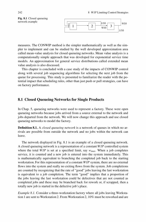
242 8 W IP Limiting Control Strategies
Fig. 8.1 Closed queueingnetwork example
1 2 39/10
1/10
1/10
9/10
measures. The CONWIP method is the simpler mathematically as well as the sim-pler to implement and can be studied by the well developed approximation areacalled mean-value analysis for closed queueing networks. Mean value analysis is acomputationally simple approach that was developed for exponential service timemodels. An approximation for general service distributions called extended meanvalue analysis is also discussed.
This chapter is concluded with a case study of the impacts of CONWIP controlalong with several job sequencing algorithms for selecting the next job from thequeue for processing. This study is presented to familiarize the reader with the po-tential impact that scheduling rules, other than just push or pull strategies, can haveon factory performance.
8.1 Closed Queueing Networks for Single Products
In Chap. 5, queueing networks were used to represent a factory. These were openqueueing networks because jobs arrived from a source external to the network andjobs departed from the network. We will now change this approach and use closedqueueing networks to model the factory.
Definition 8.1. A closed queueing network is a network of queues in which no ar-rivals are possible from outside the network and no jobs within the network canleave.
The network displayed in Fig. 8.1 is an example of a closed queueing network.A closed queueing network is a representation of a constant W IP controlled systemwhere the total WIP is set at a specified limit, say wmax. When a job completesservice, it is counted and a new job is entered into the system immediately. Thisis mathematically equivalent to branching the completed job back to the startingworkstation. For this representation of a constant WIP system, there are no externalflows into the system and really no exiting flows from the system. Job completionsare counted by recognizing that the rate of “good” jobs leaving the last workstationis equivalent to a job completion. The term “good” implies that a proportion ofthe jobs leaving the last workstation could be defectives that are not counted ascompleted jobs and these may be branched back for rework or, if scrapped, then atotally new job is started in the defective job’s place.
Example 8.1. Consider a three-workstation factory where all jobs leaving Worksta-tion 1 are sent to Workstation 2. From Workstation 2, 10% must be reworked and are
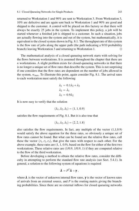
8.1 Closed Queueing Networks for Single Products 243
returned to Workstation 1 and 90% are sent to Workstation 3. From Workstation 3,10% are defective and are again sent back to Workstation 1 and 90% are good andshipped to the customer. A control will be placed on this factory so that there willalways be exactly 25 jobs in the system. To implement this policy, a job will bestarted whenever a finished job is shipped to a customer. In such a situation, jobsare actually flowing into the system and out of the system, but mathematically, it isequivalent to the closed system shown in Fig. 8.1. The throughput rate of this systemis the flow rate of jobs along the upper path (the path indicating a 9/10 probabilitybranch) leaving Workstation 3 and returning to Workstation 1. ��
The mathematical analysis of a closed queueing network starts with solving forthe flows between workstations. It is assumed throughout the chapter that there aren workstations. A slight problem exists for closed-queueing networks in that thereis no longer a unique set of flow rates that describe the system. This is not surprisingif one considers that the flow rates are dependent on the number of jobs allowed inthe system, wmax. To illustrate this point, again consider Fig. 8.1. The arrival ratesto each workstation must satisfy the following
λ1 = 0.1λ2 +λ3
λ2 = λ1
λ3 = 0.9λ2
It is now easy to verify that the solution
(λ1,λ2,λ3) = (1,1,0.9)
satisfies the flow requirements of Fig. 8.1. But it is also true that
(λ1,λ2,λ3) = (2,2,1.8)
also satisfies the flow requirements. In fact, any multiple of the vector (1,1,0.9)would satisfy the above equation for the three rates, so obviously a unique set offlow rates cannot be found. But what can be found are the relative flow rates, callthese the vector (r1, r2, r3), that give the rates with respect to each other. For theabove example, these rates are (1, 1, 0.9), based on the flow for either of the first twoworkstations. These relative rates are (1/0.9, 1/0.9, 1) if they are computed relativeto the flow of the third workstation.
Before developing a method to obtain the relative flow rates, consider the diffi-culty in attempting to perform the standard flow rate analysis (see Sect. 5.4.1). Ingeneral, a solution to the following system of equations is required
λλλ = PT λλλ +γγγ ,
where λλλ is the vector of unknown internal flow rates, γγγ is the vector of known ratesof arrivals from an external source, and P is the routing matrix giving the branch-ing probabilities. Since there are no external inflows for closed queueing networks
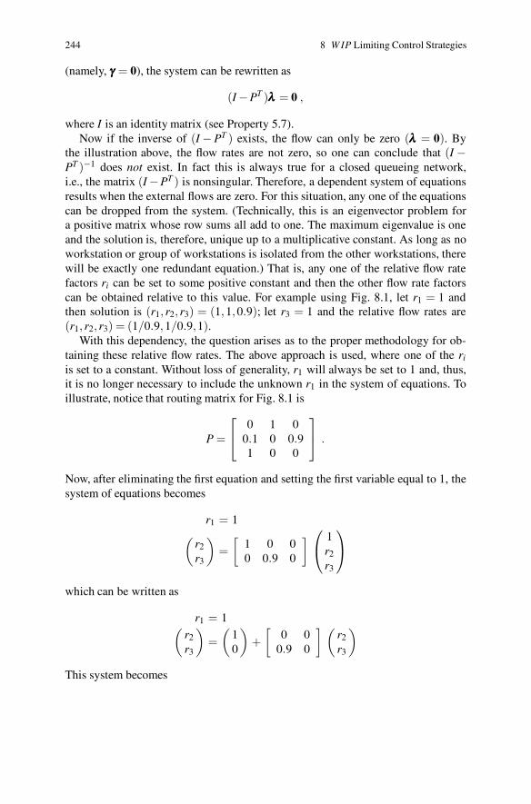
244 8 W IP Limiting Control Strategies
(namely, γγγ = 0), the system can be rewritten as
(I −PT )λλλ = 0 ,
where I is an identity matrix (see Property 5.7).Now if the inverse of (I − PT ) exists, the flow can only be zero (λλλ = 0). By
the illustration above, the flow rates are not zero, so one can conclude that (I −PT )−1 does not exist. In fact this is always true for a closed queueing network,i.e., the matrix (I −PT ) is nonsingular. Therefore, a dependent system of equationsresults when the external flows are zero. For this situation, any one of the equationscan be dropped from the system. (Technically, this is an eigenvector problem fora positive matrix whose row sums all add to one. The maximum eigenvalue is oneand the solution is, therefore, unique up to a multiplicative constant. As long as noworkstation or group of workstations is isolated from the other workstations, therewill be exactly one redundant equation.) That is, any one of the relative flow ratefactors ri can be set to some positive constant and then the other flow rate factorscan be obtained relative to this value. For example using Fig. 8.1, let r1 = 1 andthen solution is (r1, r2, r3) = (1,1,0.9); let r3 = 1 and the relative flow rates are(r1, r2, r3) = (1/0.9,1/0.9,1).
With this dependency, the question arises as to the proper methodology for ob-taining these relative flow rates. The above approach is used, where one of the ri
is set to a constant. Without loss of generality, r1 will always be set to 1 and, thus,it is no longer necessary to include the unknown r1 in the system of equations. Toillustrate, notice that routing matrix for Fig. 8.1 is
P =
⎡
⎣
0 1 00.1 0 0.91 0 0
⎤
⎦ .
Now, after eliminating the first equation and setting the first variable equal to 1, thesystem of equations becomes
r1 = 1(
r2
r3
)
=[
1 0 00 0.9 0
]
⎛
⎝
1r2
r3
⎞
⎠
which can be written as
r1 = 1(
r2
r3
)
=(
10
)
+[
0 00.9 0
] (
r2
r3
)
This system becomes

8.1 Closed Queueing Networks for Single Products 245
r1 = 1(
r2
r3
)
=([
1 00 1
]
−[
0 00.9 0
])−1(10
)
,
yielding (r1, r2, r3) = (1,1,0.9).This same logic can be extended to a general closed network resulting in the
following general property.
Property 8.1. Let P denote the routing matrix associated with a closed queue-ing network containing n workstations, and let Q denote the submatrixformed from P by deleting the first row and first column; that is, qi, j =pi+1, j+1 for i, j = 1, · · · ,n− 1. Then the vector of relative arrival rates toeach workstation, r, is given by r1 = 1 and
⎛
⎜
⎝
r2...
rn
⎞
⎟
⎠=(
I −QT)−1
⎛
⎜
⎝
p1,2...
p1,n
⎞
⎟
⎠.
Notice that I is an identity matrix of dimension n−1×n−1 and the column vectoron the right-hand side of the equation is the first row of the routing matrix minus thefirst element.
• Suggestion: Do Problems 8.1 and 8.2.
8.1.1 Analysis with Exponential Processing Times
In this section, a system of equations for determining the mean cycle time and theexpected WIP in each workstation is developed under the assumption that all pro-cessing times are exponentially distributed. The approach used when all worksta-tions have only one server and there is only one product within the factory serves asthe building block for the more complicated cases; therefore we discuss the simplestcase first and then extend those models to the other cases.
8.1.1.1 Single-Server Systems
The methodology used to determine mean cycle times within a closed network iscalled a mean value analysis. In the initial models of queueing systems, the approachwas to obtain the probability distribution for the number of jobs within the system,and then from the number of jobs, the various measures were obtained. We now
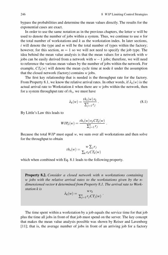
246 8 W IP Limiting Control Strategies
bypass the probabilities and determine the mean values directly. The results for theexponential cases are exact.
In order to use the same notation as in the previous chapters, the letter w will beused to denote the number of jobs within a system. Thus, we continue to use n forthe total number of workstations and k as the workstation index. In later sections,i will denote the type and m will be the total number of types within the factory;however, for this section, m = 1 so we will not need to specify the job type. Theidea behind the mean value analysis is that the mean values for a network with wjobs can be easily derived from a network with w−1 jobs; therefore, we will needto reference the various mean values by the number of jobs within the network. Forexample, CTk(w) will denote the mean cycle time at node k under the assumptionthat the closed network (factory) contains w jobs.
The first key relationship that is needed is the throughput rate for the factory.From Property 8.1, we know the relative arrival rates. In other words, if λk(w) is theactual arrival rate to Workstation k when there are w jobs within the network, thenfor a system throughput rate of ths, we must have
λk(w) =ths(w) rk
∑nj=1 r j
. (8.1)
By Little’s Law this leads to
WIPk(w) =ths(w) rk CTk(w)
∑nj=1 r j
.
Because the total WIP must equal w, we sum over all workstations and then solvefor the throughput to obtain
ths(w) =w ∑ j r j
∑k rk CTk(w)
which when combined with Eq. 8.1 leads to the following property.
Property 8.2. Consider a closed network with n workstations containingw jobs with the relative arrival rates to the workstations given by the n-dimensioned vector r determined from Property 8.1. The arrival rate to Work-station k is
λk(w) =w rk
∑nj=1 r j CTj(w)
.
The time spent within a workstation by a job equals the service time for that jobplus the time all jobs in front of that job must spend on the server. The key conceptthat makes the mean value analysis possible was shown by Reiser and Lavenberg[11]; that is, the average number of jobs in front of an arriving job for a factory
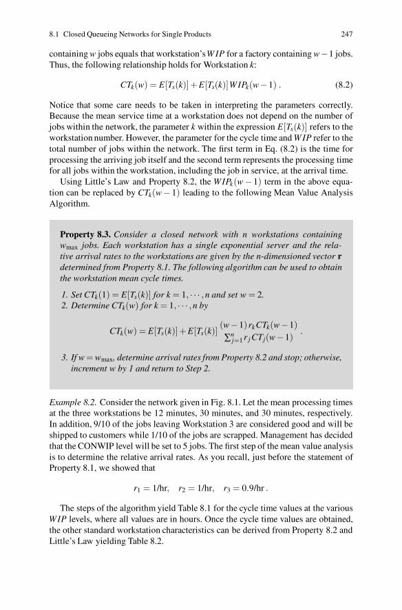
8.1 Closed Queueing Networks for Single Products 247
containing w jobs equals that workstation’sW IP for a factory containing w−1 jobs.Thus, the following relationship holds for Workstation k:
CTk(w) = E[Ts(k)]+E[Ts(k)]WIPk(w−1) . (8.2)
Notice that some care needs to be taken in interpreting the parameters correctly.Because the mean service time at a workstation does not depend on the number ofjobs within the network, the parameter k within the expression E[Ts(k)] refers to theworkstation number. However, the parameter for the cycle time and W IP refer to thetotal number of jobs within the network. The first term in Eq. (8.2) is the time forprocessing the arriving job itself and the second term represents the processing timefor all jobs within the workstation, including the job in service, at the arrival time.
Using Little’s Law and Property 8.2, the WIPk(w− 1) term in the above equa-tion can be replaced by CTk(w− 1) leading to the following Mean Value AnalysisAlgorithm.
Property 8.3. Consider a closed network with n workstations containingwmax jobs. Each workstation has a single exponential server and the rela-tive arrival rates to the workstations are given by the n-dimensioned vector rdetermined from Property 8.1. The following algorithm can be used to obtainthe workstation mean cycle times.
1. Set CTk(1) = E[Ts(k)] for k = 1, · · · ,n and set w = 2.2. Determine CTk(w) for k = 1, · · · ,n by
CTk(w) = E[Ts(k)]+E[Ts(k)](w−1) rkCTk(w−1)∑n
j=1 r j CTj(w−1).
3. If w = wmax, determine arrival rates from Property 8.2 and stop; otherwise,increment w by 1 and return to Step 2.
Example 8.2. Consider the network given in Fig. 8.1. Let the mean processing timesat the three workstations be 12 minutes, 30 minutes, and 30 minutes, respectively.In addition, 9/10 of the jobs leaving Workstation 3 are considered good and will beshipped to customers while 1/10 of the jobs are scrapped. Management has decidedthat the CONWIP level will be set to 5 jobs. The first step of the mean value analysisis to determine the relative arrival rates. As you recall, just before the statement ofProperty 8.1, we showed that
r1 = 1/hr, r2 = 1/hr, r3 = 0.9/hr .
The steps of the algorithm yield Table 8.1 for the cycle time values at the variousWIP levels, where all values are in hours. Once the cycle time values are obtained,the other standard workstation characteristics can be derived from Property 8.2 andLittle’s Law yielding Table 8.2.
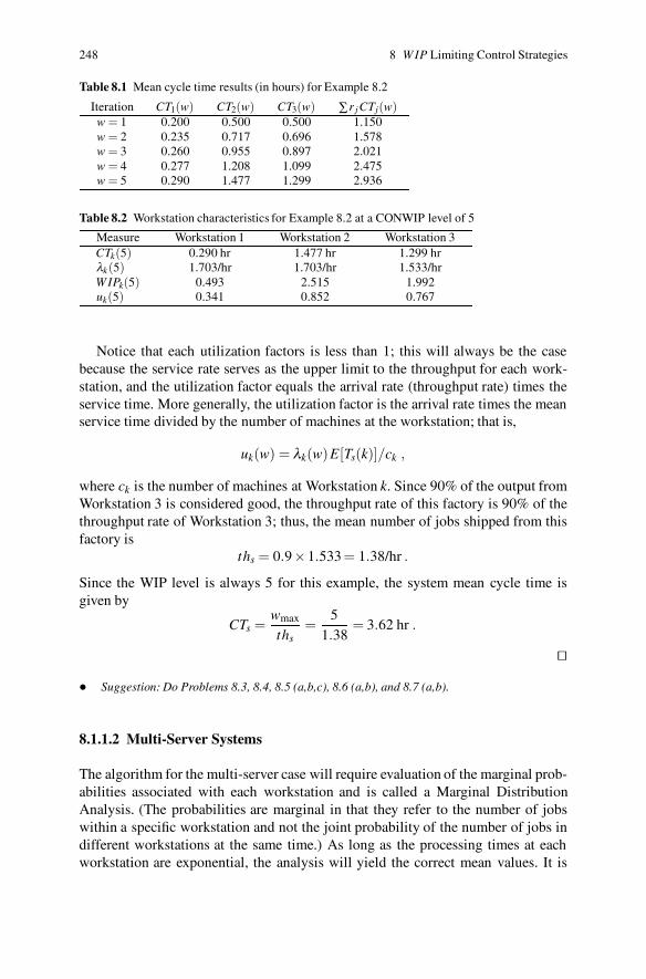
248 8 W IP Limiting Control Strategies
Table 8.1 Mean cycle time results (in hours) for Example 8.2
Iteration CT1(w) CT2(w) CT3(w) ∑r jCTj(w)w = 1 0.200 0.500 0.500 1.150w = 2 0.235 0.717 0.696 1.578w = 3 0.260 0.955 0.897 2.021w = 4 0.277 1.208 1.099 2.475w = 5 0.290 1.477 1.299 2.936
Table 8.2 Workstation characteristics for Example 8.2 at a CONWIP level of 5
Measure Workstation 1 Workstation 2 Workstation 3CTk(5) 0.290 hr 1.477 hr 1.299 hrλk(5) 1.703/hr 1.703/hr 1.533/hrW IPk(5) 0.493 2.515 1.992uk(5) 0.341 0.852 0.767
Notice that each utilization factors is less than 1; this will always be the casebecause the service rate serves as the upper limit to the throughput for each work-station, and the utilization factor equals the arrival rate (throughput rate) times theservice time. More generally, the utilization factor is the arrival rate times the meanservice time divided by the number of machines at the workstation; that is,
uk(w) = λk(w)E[Ts(k)]/ck ,
where ck is the number of machines at Workstation k. Since 90% of the output fromWorkstation 3 is considered good, the throughput rate of this factory is 90% of thethroughput rate of Workstation 3; thus, the mean number of jobs shipped from thisfactory is
ths = 0.9×1.533 = 1.38/hr .
Since the WIP level is always 5 for this example, the system mean cycle time isgiven by
CTs =wmax
ths=
51.38
= 3.62 hr .
��
• Suggestion: Do Problems 8.3, 8.4, 8.5 (a,b,c), 8.6 (a,b), and 8.7 (a,b).
8.1.1.2 Multi-Server Systems
The algorithm for the multi-server case will require evaluation of the marginal prob-abilities associated with each workstation and is called a Marginal DistributionAnalysis. (The probabilities are marginal in that they refer to the number of jobswithin a specific workstation and not the joint probability of the number of jobs indifferent workstations at the same time.) As long as the processing times at eachworkstation are exponential, the analysis will yield the correct mean values. It is
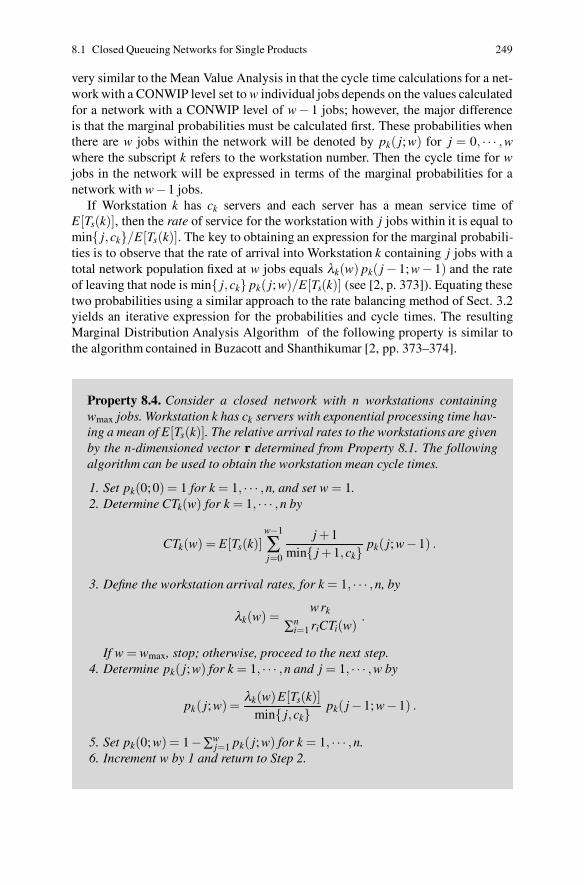
8.1 Closed Queueing Networks for Single Products 249
very similar to the Mean Value Analysis in that the cycle time calculations for a net-work with a CONWIP level set to w individual jobs depends on the values calculatedfor a network with a CONWIP level of w− 1 jobs; however, the major differenceis that the marginal probabilities must be calculated first. These probabilities whenthere are w jobs within the network will be denoted by pk( j; w) for j = 0, · · · ,wwhere the subscript k refers to the workstation number. Then the cycle time for wjobs in the network will be expressed in terms of the marginal probabilities for anetwork with w−1 jobs.
If Workstation k has ck servers and each server has a mean service time ofE[Ts(k)], then the rate of service for the workstation with j jobs within it is equal tomin{ j,ck}/E[Ts(k)]. The key to obtaining an expression for the marginal probabili-ties is to observe that the rate of arrival into Workstation k containing j jobs with atotal network population fixed at w jobs equals λk(w) pk( j − 1; w− 1) and the rateof leaving that node is min{ j,ck} pk( j; w)/E[Ts(k)] (see [2, p. 373]). Equating thesetwo probabilities using a similar approach to the rate balancing method of Sect. 3.2yields an iterative expression for the probabilities and cycle times. The resultingMarginal Distribution Analysis Algorithm of the following property is similar tothe algorithm contained in Buzacott and Shanthikumar [2, pp. 373–374].
Property 8.4. Consider a closed network with n workstations containingwmax jobs. Workstation k has ck servers with exponential processing time hav-ing a mean of E[Ts(k)]. The relative arrival rates to the workstations are givenby the n-dimensioned vector r determined from Property 8.1. The followingalgorithm can be used to obtain the workstation mean cycle times.
1. Set pk(0; 0) = 1 for k = 1, · · · ,n, and set w = 1.2. Determine CTk(w) for k = 1, · · · ,n by
CTk(w) = E[Ts(k)]w−1
∑j=0
j +1min{ j +1,ck}
pk( j; w−1) .
3. Define the workstation arrival rates, for k = 1, · · · ,n, by
λk(w) =w rk
∑ni=1 riCTi(w)
.
If w = wmax, stop; otherwise, proceed to the next step.4. Determine pk( j; w) for k = 1, · · · ,n and j = 1, · · · ,w by
pk( j; w) =λk(w)E[Ts(k)]
min{ j,ck}pk( j−1; w−1) .
5. Set pk(0; w) = 1−∑wj=1 pk( j; w) for k = 1, · · · ,n.
6. Increment w by 1 and return to Step 2.
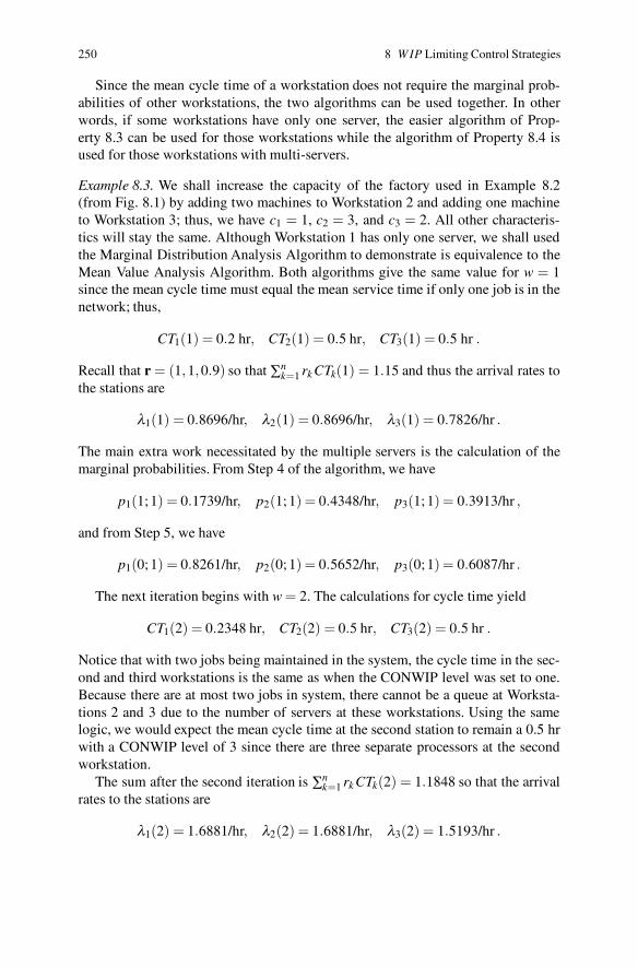
250 8 W IP Limiting Control Strategies
Since the mean cycle time of a workstation does not require the marginal prob-abilities of other workstations, the two algorithms can be used together. In otherwords, if some workstations have only one server, the easier algorithm of Prop-erty 8.3 can be used for those workstations while the algorithm of Property 8.4 isused for those workstations with multi-servers.
Example 8.3. We shall increase the capacity of the factory used in Example 8.2(from Fig. 8.1) by adding two machines to Workstation 2 and adding one machineto Workstation 3; thus, we have c1 = 1, c2 = 3, and c3 = 2. All other characteris-tics will stay the same. Although Workstation 1 has only one server, we shall usedthe Marginal Distribution Analysis Algorithm to demonstrate is equivalence to theMean Value Analysis Algorithm. Both algorithms give the same value for w = 1since the mean cycle time must equal the mean service time if only one job is in thenetwork; thus,
CT1(1) = 0.2 hr, CT2(1) = 0.5 hr, CT3(1) = 0.5 hr .
Recall that r = (1,1,0.9) so that ∑nk=1 rk CTk(1) = 1.15 and thus the arrival rates to
the stations are
λ1(1) = 0.8696/hr, λ2(1) = 0.8696/hr, λ3(1) = 0.7826/hr .
The main extra work necessitated by the multiple servers is the calculation of themarginal probabilities. From Step 4 of the algorithm, we have
p1(1; 1) = 0.1739/hr, p2(1; 1) = 0.4348/hr, p3(1; 1) = 0.3913/hr ,
and from Step 5, we have
p1(0; 1) = 0.8261/hr, p2(0; 1) = 0.5652/hr, p3(0; 1) = 0.6087/hr .
The next iteration begins with w = 2. The calculations for cycle time yield
CT1(2) = 0.2348 hr, CT2(2) = 0.5 hr, CT3(2) = 0.5 hr .
Notice that with two jobs being maintained in the system, the cycle time in the sec-ond and third workstations is the same as when the CONWIP level was set to one.Because there are at most two jobs in system, there cannot be a queue at Worksta-tions 2 and 3 due to the number of servers at these workstations. Using the samelogic, we would expect the mean cycle time at the second station to remain a 0.5 hrwith a CONWIP level of 3 since there are three separate processors at the secondworkstation.
The sum after the second iteration is ∑nk=1 rk CTk(2) = 1.1848 so that the arrival
rates to the stations are
λ1(2) = 1.6881/hr, λ2(2) = 1.6881/hr, λ3(2) = 1.5193/hr .

8.1 Closed Queueing Networks for Single Products 251
Each time the number of jobs within the factory increases, the number of calcula-tions for the marginal probabilities also increase. The probability calculations areshown in Table 8.3.
Table 8.3 Marginal probabilities for w = 2 in Example 8.3
Workstation 1 Workstation 2 Workstation 3pk(1;2) 0.2789 0.4771 0.4624pk(2;2) 0.0587 0.1835 0.1486pk(0;2) 0.6624 0.3394 0.3890
The next iteration begins with w = 3. The calculations for cycle time yield
CT1(3) = 0.2793 hr, CT2(3) = 0.5 hr, CT3(3) = 0.5372 hr .
The sum is ∑nk=1 rk CTk(3) = 1.2627 so that the arrival rates to the stations are
λ1(3) = 2.3758/hr, λ2(3) = 2.3758/hr, λ3(3) = 2.1382/hr .
Notice that the numerical value for CT1(3) is the same whether the algorithm ofProperty 8.4 or 8.3 is used, as long as the values for CT2(3) and CT3(3) come fromProperty 8.4. However, it does serve to check for numerical carelessness, so we willcontinue calculating the probabilities associated with Workstation 1. The probabilitycalculations are shown in Table 8.4.
Table 8.4 Marginal probabilities for w = 3 in Example 8.3
Workstation 1 Workstation 2 Workstation 3pk(1;3) 0.3147 0.4032 0.4159pk(2;3) 0.1325 0.2834 0.2472pk(3;3) 0.0279 0.0727 0.0794pk(0;3) 0.5248 0.2407 0.2575
The next iteration begins with w = 4. The calculations for cycle time yield
CT1(4) = 0.3327 hr, CT2(4) = 0.5121 hr, CT3(4) = 0.6015 hr .
The sum is ∑nk=1 rk CTk(4) = 1.3862 so that the arrival rates to the stations are
λ1(4) = 2.8856/hr, λ2(4) = 2.8856/hr, λ3(4) = 2.5971/hr .
The final probability calculations are shown in Table 8.5.Since our factory has a CONWIP level set at wmax = 5, the final iteration involves
only the first three steps of the algorithm. Then after the final cycle times and arrivalrates are calculated, Little’s Law can be used to obtain the workstation average W IPlevels. These final results are contained in Table 8.6.
The rate at which jobs can be shipped out of this system is
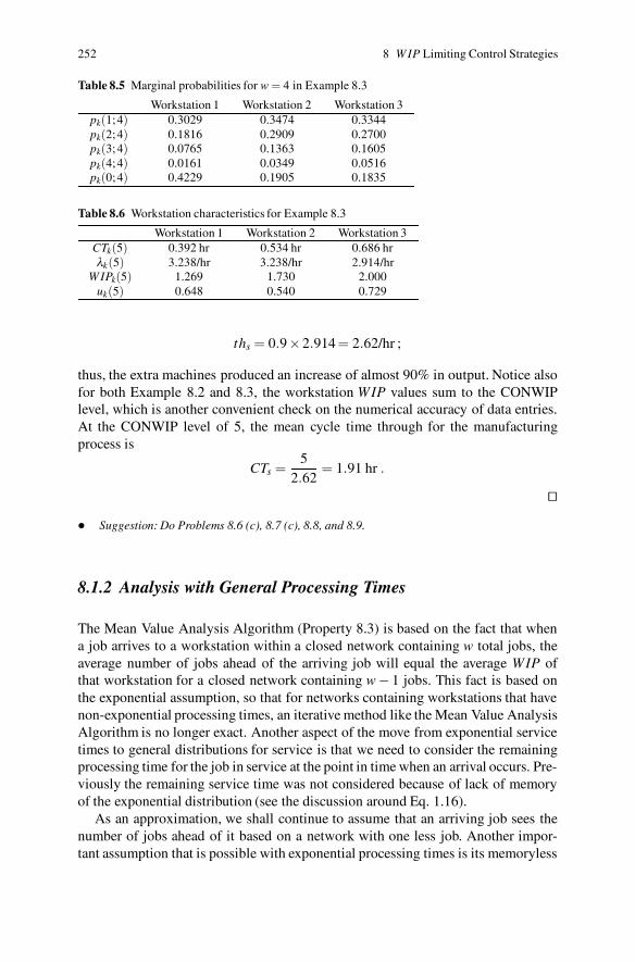
252 8 W IP Limiting Control Strategies
Table 8.5 Marginal probabilities for w = 4 in Example 8.3
Workstation 1 Workstation 2 Workstation 3pk(1;4) 0.3029 0.3474 0.3344pk(2;4) 0.1816 0.2909 0.2700pk(3;4) 0.0765 0.1363 0.1605pk(4;4) 0.0161 0.0349 0.0516pk(0;4) 0.4229 0.1905 0.1835
Table 8.6 Workstation characteristics for Example 8.3
Workstation 1 Workstation 2 Workstation 3CTk(5) 0.392 hr 0.534 hr 0.686 hrλk(5) 3.238/hr 3.238/hr 2.914/hr
W IPk(5) 1.269 1.730 2.000uk(5) 0.648 0.540 0.729
ths = 0.9×2.914 = 2.62/hr ;
thus, the extra machines produced an increase of almost 90% in output. Notice alsofor both Example 8.2 and 8.3, the workstation WIP values sum to the CONWIPlevel, which is another convenient check on the numerical accuracy of data entries.At the CONWIP level of 5, the mean cycle time through for the manufacturingprocess is
CTs =5
2.62= 1.91 hr .
��
• Suggestion: Do Problems 8.6 (c), 8.7 (c), 8.8, and 8.9.
8.1.2 Analysis with General Processing Times
The Mean Value Analysis Algorithm (Property 8.3) is based on the fact that whena job arrives to a workstation within a closed network containing w total jobs, theaverage number of jobs ahead of the arriving job will equal the average WIP ofthat workstation for a closed network containing w− 1 jobs. This fact is based onthe exponential assumption, so that for networks containing workstations that havenon-exponential processing times, an iterative method like the Mean Value AnalysisAlgorithm is no longer exact. Another aspect of the move from exponential servicetimes to general distributions for service is that we need to consider the remainingprocessing time for the job in service at the point in time when an arrival occurs. Pre-viously the remaining service time was not considered because of lack of memoryof the exponential distribution (see the discussion around Eq. 1.16).
As an approximation, we shall continue to assume that an arriving job sees thenumber of jobs ahead of it based on a network with one less job. Another impor-tant assumption that is possible with exponential processing times is its memoryless

8.1 Closed Queueing Networks for Single Products 253
property. In other words, consider a processor with first and second moments givenby E[Ts] and E[T 2
s ]. Assume that a job is undergoing processing and we pick an ar-bitrary point in time and would like to determine the mean remaining time until pro-cessing is finished for that part. For an exponential processor, the mean remainingtime is E[Ts] based on the memoryless property. For a non-exponential processor,the mean remaining time is given by E[T 2
s ]/(2E[T ]2) (see [6]). Thus, we developa modified Mean Value Analysis Algorithm by using the appropriate form for theremaining time for the job in process as seen at an arbitrary point in time.
As you recall, Eq. (8.2) was the basis for the Mean Value Analysis Algorithmand it is composed of three parts: (i) the remaining processing time for the job beingserviced (if any), (ii) a full service time for each job in the queue when the jobunder consideration arrives, and (iii) a full service time for the arriving job. Sincethe utilization factor is the probability that the processor is busy, Eq. (8.2) can bewritten as
CTk(w) = E[Ts(k)]+E[Ts(k)] (WIPk(w−1)−uk(w−1)) (8.3)
+uk(w−1)E[T2s ]/(2E[T ]) ,
where uk(w−1) is the utilization factor for Workstation k when there are a total ofw−1 jobs in the network, and from Property 8.2 we have
uk(w) =w rk E[Ts(k)]
∑nj=1 r j CTj(w)
. (8.4)
The first step in combining Eqs. (8.3) and (8.4) is to use Little’s Law to replaceWIP(w−1) with CT (w−1) in Eq. (8.3). The utilization factor is then eliminated inEq. (8.3) by using Eq. (8.4). Finally, we use the fact
E[Ts(k)2] = E[Ts(k)]2 (C2s (k)+1) (8.5)
since our data usually include the SCV instead of the second moment. After simpli-fying, the following property is obtained that modifies the mean value analysis to anapproximation procedure for non-exponential service times.
Property 8.5. Consider a closed network with n workstations containingwmax jobs. Each workstation has a single processor with processor character-istics given by E[Ts(k)] and C2
s (k) and the relative arrival rates to the worksta-tions are given by the n-dimensioned vector r determined from Property 8.1.The following algorithm can be used to obtain the workstation mean cycletimes.
1. Set CTk(1) = E[Ts(k)] for k = 1, · · · ,n and set w = 2.2. Determine CTk(w) for k = 1, · · · ,n by
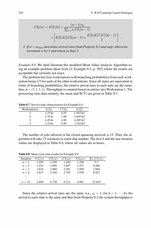
254 8 W IP Limiting Control Strategies
CTk(w) = E[Ts(k)]+(w−1) rk
∑nj=1 r j CTj(w−1)
×[
E[Ts(k)]CTk(w−1)+E[Ts(k)]2 (C2
s (k)−1)2
]
.
3. If w = wmax, determine arrival rates from Property 8.2 and stop; otherwise,increment w by 1 and return to Step 2.
Example 8.4. We shall illustrate this modified Mean Value Analysis Algorithm us-ing an example problem taken from [2, Example 8.5, p. 382] where the results areacceptable but certainly not exact.
The problem has four workstations with branching probabilities from each work-station being 1/3 for each of the other workstations. Since all states are equivalent interms of branching probabilities, the relative arrival rates to each state are the same;thus, r = (1,1,1,1). Throughput is counted based on entries into Workstation 1. Theprocessing time data (namely, the mean and SCV) are given in Table 8.7.
Table 8.7 Service time characteristics for Example 8.4
Workstation k E [Tk] C2[Tk] E [T2k ]
1 1.25 hr 0.25 1.953 hr2
2 1.35 hr 1.00 3.645 hr2
3 1.45 hr 1.00 4.205 hr2
4 1.25 hr 0.50 2.344 hr2
The number of jobs allowed in the closed queueing network is 15. Thus, the al-gorithm will take 15 iterations to reach that number. The first 4 and the last iterationvalues are displayed in Table 8.8, where all values are in hours.
Table 8.8 Mean cycle time results for Example 8.4
Iteration CT1(w) CT2(w) CT3(w) CT4(w) ∑r j CTj(w)w = 1 1.250 1.350 1.450 1.250 5.3w = 2 1.434 1.694 1.847 1.471 6.446w = 3 1.624 2.060 2.281 1.699 7.664w = 4 1.815 2.438 2.745 1.929 8.927
......
......
......
w = 15 3.609 6.738 9.231 4.081 23.659
Since the relative arrival rates are the same (i.e., rk = 1, for k = 1, · · · ,4), thearrival to each state is the same and thus from Property 8.2 the system throughput is

8.2 Closed Queueing Networks with Multiple Products 255
th(15) = λ1(15) =15× r1
∑4j=1 r j CTj
=15
23.659= 0.634/hr .
The throughput estimation for this system agrees to three decimal places with thesimulation results of [2]. The cycle time results, however, are not as impressive.If we assume that the simulation results contained in [2] for this example are theexact values, then the percent errors in the mean cycle time estimates for the fourworkstations are -13.0%, 4.9%, 5.1%, and -4.6%. Thus, for non-exponential servicetimes, the algorithm of Property 8.5 yields acceptable but far from perfect results.However, if we naively used the exponential assumption by following Property 8.3,the errors for the four workstations would be 30.3%, 15.4%, 18.7%, and 26%; thus,if the service time SCV is not 1, it is best to take advantage of the modified versionof the Mean Value Analysis. ��
• Suggestion: Do Problems 8.10 and 8.11.
8.2 Closed Queueing Networks with Multiple Products
It is not too difficult to extend the (single-server) Mean Value Analysis Algorithmto account for multiple products; however, the implementation of the algorithm be-comes intractable with more than just a couple of products and modest CONWIPlevels.
As in Chap. 6, notation will become more cumbersome since there are morequantities that must be reflected in the notation. For the most part, we will be ableto use similar notation as was used in Chap. 6; namely, the index i will be used forthe job type (product) and it will often be written as a superscript. The total numberof job types will be m.
Each job type will have its own routing matrix and thus its own relative arrivalrates which will be denoted by the vector ri = (ri,1, · · · , ri,n). The value of ri isdetermined by Property 8.1, where the matrix P and submatrix Q of the propertyare replaced by the routing matrix Pi and submatrix Qi that describe the switchingprobabilities associated with Job Type i.
With multiple job types, a separate CONWIP level must be specified for eachtype. In other words, when a Type i job is finished, another Type i will be started.Since we assume that there are m different job types, the CONWIP level is a vectorcalled w = (w1, · · · ,wm). The vector ei is used to specify the unit vector with a onein the i-position and zeros elsewhere. The unit vector is used to indicate a decrease(or increase) of one unit of a specified job type. For example, the vector w − e1
represents a CONWIP level specified by w except with one less of Type 1; thus,w− e1 = (w1 −1,w2, · · · ,wm).
In the next section, the Mean Value Analysis Algorithm will be extended and asmall example will be used to demonstrate its implementation. Then in Sect. 8.2.2 anapproximation will be derived that gives a much easier implementation with reason-able results as long as the total CONWIP level is not too small. Finally, in Sect. 8.2.3
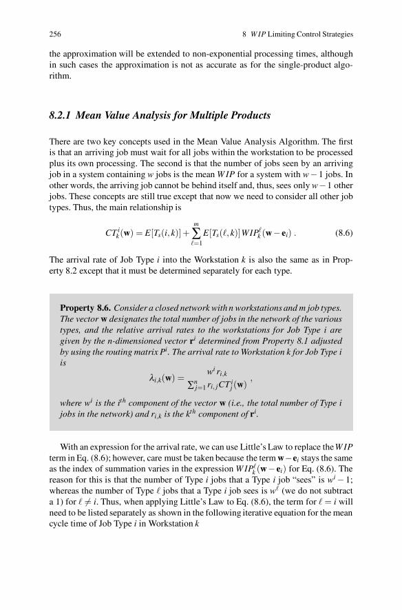
256 8 W IP Limiting Control Strategies
the approximation will be extended to non-exponential processing times, althoughin such cases the approximation is not as accurate as for the single-product algo-rithm.
8.2.1 Mean Value Analysis for Multiple Products
There are two key concepts used in the Mean Value Analysis Algorithm. The firstis that an arriving job must wait for all jobs within the workstation to be processedplus its own processing. The second is that the number of jobs seen by an arrivingjob in a system containing w jobs is the mean W IP for a system with w−1 jobs. Inother words, the arriving job cannot be behind itself and, thus, sees only w−1 otherjobs. These concepts are still true except that now we need to consider all other jobtypes. Thus, the main relationship is
CT ik(w) = E[Ts(i,k)]+
m
∑�=1
E[Ts(�,k)]WIP�k (w− ei) . (8.6)
The arrival rate of Job Type i into the Workstation k is also the same as in Prop-erty 8.2 except that it must be determined separately for each type.
Property 8.6. Consider a closed network with n workstations and m job types.The vector w designates the total number of jobs in the network of the varioustypes, and the relative arrival rates to the workstations for Job Type i aregiven by the n-dimensioned vector ri determined from Property 8.1 adjustedby using the routing matrix Pi. The arrival rate to Workstation k for Job Type iis
λi,k(w) =wi ri,k
∑nj=1 ri, jCT i
j (w),
where wi is the ith component of the vector w (i.e., the total number of Type ijobs in the network) and ri,k is the kth component of ri.
With an expression for the arrival rate, we can use Little’s Law to replace theW IPterm in Eq. (8.6); however, care must be taken because the term w−ei stays the sameas the index of summation varies in the expression W IP�
k (w− ei) for Eq. (8.6). Thereason for this is that the number of Type i jobs that a Type i job “sees” is wi − 1;whereas the number of Type � jobs that a Type i job sees is w� (we do not subtracta 1) for � �= i. Thus, when applying Little’s Law to Eq. (8.6), the term for � = i willneed to be listed separately as shown in the following iterative equation for the meancycle time of Job Type i in Workstation k

8.2 Closed Queueing Networks with Multiple Products 257
CT ik (w) = E[Ts(i,k)]+E[Ts(i,k)]
(wi −1) ri,kCT ik (w− ei)
∑nj=1 ri, jCT i
j(w− ei)
+m
∑�=1� �=i
E[Ts(�,k)]w� r�,kCT �
k (w− ei)∑n
j=1 r�, jCT �j (w− ei)
, (8.7)
where w� is the total number of Type � jobs within the closed network, and theexpression that is written as a ratio is evaluated to zero if the numerator is zero, eventhough the denominator will also be zero. Conceptually, Eq. (8.7) is very similarto the iterative expression in Property 8.3; however, implementation is significantlyworse because of the necessity to determine the cycle time for all combinations ofthe vector w whose individual components are less that their maximum value. Indeveloping the next algorithm, we shall let wmax denote the vector (w1
max, · · · ,wmmax)
so that it is possible for each component to have its own maximum value. We alsolet 0 denote an m-dimensioned vector of all zeros. Finally, we let |w| = ∑m
i=1 |wi|.
Property 8.7. Consider a closed network with n workstations, m job types,and wmax designating the total number of jobs in the network of the varioustypes. Each workstation has a single exponential server and the relative ar-rival rates to the workstations for Job Type i are given by the n-dimensionedvector ri. The following algorithm can be used to obtain the mean cycle timesfor Type i jobs at Workstation k.
1. Set CT ik (0) = 0 and CT i
k(ei) = E[Ts(i,k)] for k = 1, · · · ,n and i = 1, · · · ,m.Set W = 2.
2. For each w such that |w| = W and each wi ≤ wmax, determine CTik(w) for
i = 1, · · · ,m and k = 1, · · · ,n from Eq. (8.7).3. If W = |wmax| = ∑m
i=1 wmax, determine all arrival rates from Property 8.6with w = wmax and stop; otherwise, increment W by 1 and return to Step 2.
Once the arrival rates have been determined, the WIP in each station for each jobtype can be determined and as a check for numerical accuracy, the sum of the W IPshould equal |wmax|. Step 2 contains several “sub-steps” since there will be severalvectors w that satisfy the stated condition, and the order in which the cycle timesare evaluated is important. Whenever a value of CT i
k (w) is to be calculated, it isimportant that the value of CT i
k (w−ei) has already been determined. To insure this,the algorithm should proceed through the possible values of w in either lexicograph-ical order or reverse lexicographical order. (Lexicographical order is the order in adictionary; thus (2,5,3,0) comes before (3,0,2,7) in lexicographical order.)
Example 8.5. Consider a manufacturing facility that has three workstations, witha single machine in each workstation. There are two products that are producedsimultaneously in the factory. The workstation flow diagram for each product are
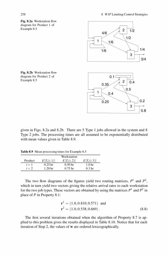
258 8 W IP Limiting Control Strategies
Fig. 8.2a Workstation flowdiagram for Product 1 ofExample 8.5
1
2
3
4/6
1/6
1/4
3/4
1/2
1/2
1/6
Fig. 8.2b Workstation flowdiagram for Product 2 ofExample 8.5
1
2
3
0.35
0.4
0.25 0.2
0.8
0.5
0.4
0.1
given in Figs. 8.2a and 8.2b. There are 5 Type 1 jobs allowed in the system and 8Type 2 jobs. The processing times are all assumed to be exponentially distributedwith mean values given in Table 8.9.
Table 8.9 Mean processing times for Example 8.5
WorkstationProduct E [Ts(i,1)] E [Ts(i,2)] E [Ts(i,3)]
i = 1 0.25 hr 0.50 hr 1.0 hri = 2 1.20 hr 0.75 hr 0.3 hr
The two flow diagrams of the figures yield two routing matrices, P1 and P2,which in turn yield two vectors giving the relative arrival rates to each workstationfor the two job types. These vectors are obtained by using the matrices P1 and P2 inplace of P in Property 8.1:
r1 = (1.0,0.810,0.571) and
r2 = (1.0,0.538,0.669) . (8.8)
The first several iterations obtained when the algorithm of Property 8.7 is ap-plied to this problem gives the results displayed in Table 8.10. Notice that for eachiteration of Step 2, the values of w are ordered lexicographically.
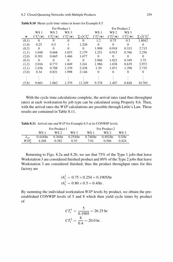
8.2 Closed Queueing Networks with Multiple Products 259
Table 8.10 Mean cycle time values in hours for Example 8.5
For Product 1 For Product 2WS 1 WS 2 WS 3 WS 1 WS 2 WS 3
w CT 11 (w) CT1
2 (w) CT13 (w) ∑r1
kCT1k CT2
1 (w) CT 22 (w) CT 2
3 (w) ∑r2kCT 2
k(0,1) 0 0 0 0 1.2 0.75 0.3 1.8042(1,0) 0.25 0.5 1 1.226 0 0 0 0(0,2) 0 0 0 0 1.998 0.918 0.333 2.715(1,1) 1.048 0.668 1.033 2.179 1.251 0.915 0.766 2.256(2,0) 0.301 0.665 1.466 1.677 0 0 0 0(0,3) 0 0 0 0 2.966 1.023 0.349 3.75(1,2) 2.016 0.773 1.049 3.241 1.986 1.038 0.639 2.972(2,1) 1.036 0.788 1.339 2.438 1.29 1.071 1.298 2.735(3,0) 0.34 0.821 1.998 2.146 0 0 0 0
......
......
......
......
...(5,8) 9.601 1.062 1.379 11.249 9.378 1.407 0.848 10.701
With the cycle time calculations complete, the arrival rates (and thus throughputrates) at each workstation by job type can be calculated using Property 8.6. Then,with the arrival rates the W IP calculations are possible through Little’s Law. Theseresults are contained in Table 8.11.
Table 8.11 Arrival rate and W IP for Example 8.5 at its CONWIP levels
For Product 1 For Product 2WS 1 WS 2 WS 3 WS 1 WS 2 WS 3
λi,k 0.444/hr 0.36/hr 0.254/hr 0.748/hr 0.402/hr 0.5/hrW IPi
k 4.268 0.382 0.35 7.01 0.566 0.424
Returning to Figs. 8.2a and 8.2b, we see that 75% of the Type 1 jobs that leaveWorkstation 3 are considered finished product and 80% of the Type 2 jobs that leaveWorkstation 3 are considered finished; thus the product throughput rates for thisfactory are
th1s = 0.75×0.254 = 0.1905/hr
th2s = 0.80×0.5 = 0.4/hr .
By summing the individual workstation WIP levels by product, we obtain the pre-established CONWIP levels of 5 and 8 which then yield cycle times by productof
CT 1s =
50.1905
= 26.25 hr
CT 2s =
80.4
= 20.0 hr .
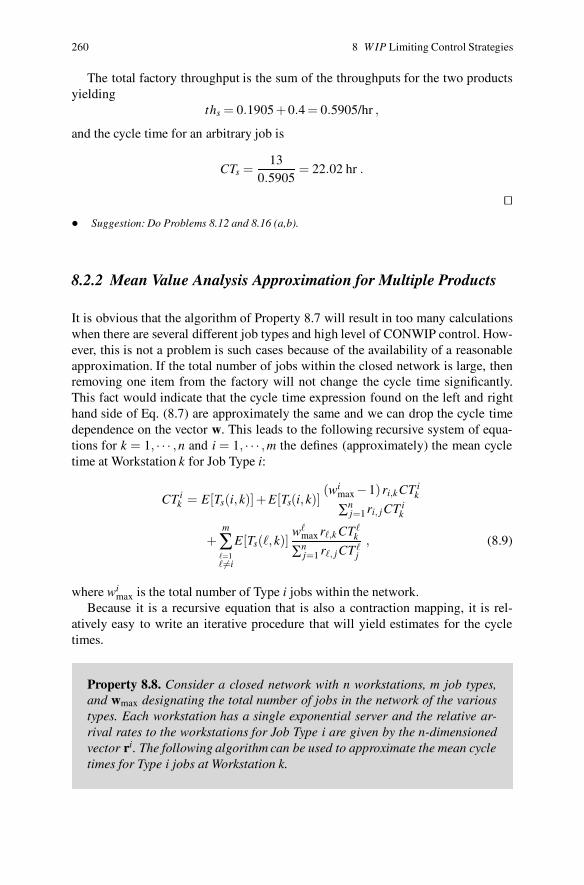
260 8 W IP Limiting Control Strategies
The total factory throughput is the sum of the throughputs for the two productsyielding
ths = 0.1905 +0.4 = 0.5905/hr ,
and the cycle time for an arbitrary job is
CTs =13
0.5905= 22.02 hr .
��• Suggestion: Do Problems 8.12 and 8.16 (a,b).
8.2.2 Mean Value Analysis Approximation for Multiple Products
It is obvious that the algorithm of Property 8.7 will result in too many calculationswhen there are several different job types and high level of CONWIP control. How-ever, this is not a problem is such cases because of the availability of a reasonableapproximation. If the total number of jobs within the closed network is large, thenremoving one item from the factory will not change the cycle time significantly.This fact would indicate that the cycle time expression found on the left and righthand side of Eq. (8.7) are approximately the same and we can drop the cycle timedependence on the vector w. This leads to the following recursive system of equa-tions for k = 1, · · · ,n and i = 1, · · · ,m the defines (approximately) the mean cycletime at Workstation k for Job Type i:
CT ik = E[Ts(i,k)]+E[Ts(i,k)]
(wimax−1) ri,kCT i
k
∑nj=1 ri, jCT i
k
+m
∑�=1� �=i
E[Ts(�,k)]w�
max r�,k CT �k
∑nj=1 r�, jCT �
j
, (8.9)
where wimax is the total number of Type i jobs within the network.
Because it is a recursive equation that is also a contraction mapping, it is rel-atively easy to write an iterative procedure that will yield estimates for the cycletimes.
Property 8.8. Consider a closed network with n workstations, m job types,and wmax designating the total number of jobs in the network of the varioustypes. Each workstation has a single exponential server and the relative ar-rival rates to the workstations for Job Type i are given by the n-dimensionedvector ri. The following algorithm can be used to approximate the mean cycletimes for Type i jobs at Workstation k.

8.2 Closed Queueing Networks with Multiple Products 261
1. Set CT ik,old = E[Ts(i,k)] for k = 1, · · · ,n and i = 1, · · · ,m.
2. For each k = 1, · · · ,n and i = 1, · · · ,m, obtain values for CT ik,new by using
Eq. (8.9) with the CT ik,old values used for the right-hand side cycle time
values and the CT ik,new values are from the left-hand side.
3. Let the error term be defined as maxi,k{|CTik,new−CT i
k,old|}, and if the er-
ror term is less than 10−5 (or other chosen limit), stop; otherwise, let theCT i
k,old values become the CT ik,new values and repeat Step 2.
Example 8.6. Consider again the manufacturing facility of Example 8.5 and illus-trated with Figs. 8.2a and 8.2b. Using the values from Table 8.9 and Eq. (8.8) weget the following iteration, where all values are in hours.
Table 8.12 Mean cycle time values in hours for Example 8.6
For Product 1 For Product 2WS 1 WS 2 WS 3 WS 1 WS 2 WS 3
Iteration # CT 11 CT 1
2 CT13 ∑r1
kCT 1k CT 2
1 CT22 CT 2
3 ∑r2kCT2
k1 0.25 0.5 1 1.226 1.2 0.75 0.3 1.80422 6.839 2.5026 3.1299 10.6533 7.0419 2.75 2.8623 10.43623 7.3696 1.7311 2.1114 9.9774 7.6704 1.97 1.5241 9.74984 8.5411 1.4333 1.7343 10.6924 8.7317 1.672 1.1238 10.3831...
......
......
......
......
15 9.6747 1.0166 1.3911 11.2925 9.7679 1.2567 0.7477 10.9443
Table 8.13 Arrival rate and W IP for Example 8.5 at its CONWIP levels of 5 and 8
For Product 1 For Product 2WS 1 WS 2 WS 3 WS 1 WS 2 WS 3
λ ik 0.4428/hr 0.3586/hr 0.2528/hr 0.731/hr 0.3933/hr 0.489/hr
W IPik 4.2837 0.3646 0.3517 7.1401 0.4942 0.3656
Since 75% of the Type 1 jobs that leave Workstation 3 are considered finishedproduct and 80% of the Type 2 jobs that leave Workstation 3 are considered finished,the product throughput rates for this factory are
th1s = 0.75×0.2528 = 0.1896/hr
th2s = 0.80×0.489 = 0.3912/hr .
By summing the individual workstation WIP levels by product, we obtain the pre-established CONWIP levels of 5 and 8 which then yield cycle times by productof
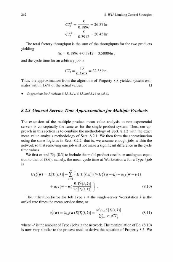
262 8 W IP Limiting Control Strategies
CT 1s =
50.1896
= 26.37 hr
CT 2s =
80.3912
= 20.45 hr
The total factory throughput is the sum of the throughputs for the two productsyielding
ths = 0.1896 +0.3912 = 0.5808/hr ,
and the cycle time for an arbitrary job is
CTs =13
0.5808= 22.38 hr .
Thus, the approximation from the algorithm of Property 8.8 yielded system esti-mates within 1.6% of the actual values. ��
• Suggestion: Do Problems 8.13, 8.14, 8.15, and 8.16 (a,c,d,e).
8.2.3 General Service Time Approximation for Multiple Products
The extension of the multiple product mean value analysis to non-exponentialservers is conceptually the same as for the single product system. Thus, our ap-proach in this section is to combine the methodology of Sect. 8.1.2 with the exactmean value analysis methodology of Sect. 8.2.1. We then form the approximationusing the same logic as in Sect. 8.2.2; that is, we assume enough jobs within thenetwork so that removing one job will not make a significant difference in the cycletime values.
We first extend Eq. (8.3) to include the multi-product case in an analogous equa-tion to that of (8.6); namely, the mean cycle time at Workstation k for a Type i jobis
CT ik(w) = E[Ts(i,k)]+
m
∑�=1
{
E[Ts(�,k)] (WIP�k (w− ei)−u�,k(w− ei) )
+ u�,k(w− ei)E[T 2
s (�,k)]2E[Ts(�,k)]
}
. (8.10)
The utilization factor for Job Type i at the single-server Workstation k is thearrival rate times the mean service time, or
uik(w) = λi,k(w)E[Ts(i,k)] =
wi ri,k E[Ts(i,k)]∑n
j=1 ri, jCT ij
, (8.11)
where wi is the amount of Type i jobs in the network. The manipulation of Eq. (8.10)is now very similar to the process used to derive the equation of Property 8.5. We
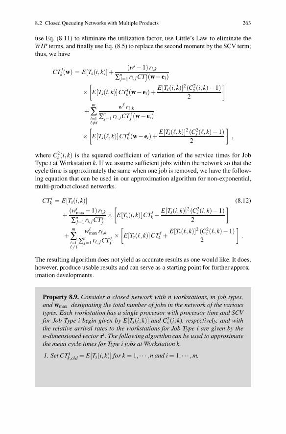
8.2 Closed Queueing Networks with Multiple Products 263
use Eq. (8.11) to eliminate the utilization factor, use Little’s Law to eliminate theWIP terms, and finally use Eq. (8.5) to replace the second moment by the SCV term;thus, we have
CT ik(w) = E[Ts(i,k)]+
(wi −1) ri,k
∑nj=1 ri, jCT i
j (w− ei)
×[
E[Ts(i,k)]CTik(w− ei)+
E[Ts(i,k)]2(C2s (i,k)−1)
2
]
+m
∑�=1� �=i
w� r�,k
∑nj=1 r�, jCT �
j (w− ei)
×[
E[Ts(�,k)]CT �k (w− ei)+
E[Ts(�,k)]2 (C2s (�,k)−1)
2
]
,
where C2s (i,k) is the squared coefficient of variation of the service times for Job
Type i at Workstation k. If we assume sufficient jobs within the network so that thecycle time is approximately the same when one job is removed, we have the follow-ing equation that can be used in our approximation algorithm for non-exponential,multi-product closed networks.
CT ik = E[Ts(i,k)] (8.12)
+(wi
max −1) ri,k
∑nj=1 ri, jCT i
j
×[
E[Ts(i,k)]CTik +
E[Ts(i,k)]2(C2s (i,k)−1)
2
]
+m
∑�=1� �=i
w�max r�,k
∑nj=1 r�, jCT �
j
×[
E[Ts(�,k)]CT �k +
E[Ts(�,k)]2 (C2s (�,k)−1)
2
]
.
The resulting algorithm does not yield as accurate results as one would like. It does,however, produce usable results and can serve as a starting point for further approx-imation developments.
Property 8.9. Consider a closed network with n workstations, m job types,and wmax designating the total number of jobs in the network of the varioustypes. Each workstation has a single processor with processor time and SCVfor Job Type i begin given by E[Ts(i,k)] and C2
s (i,k), respectively, and withthe relative arrival rates to the workstations for Job Type i are given by then-dimensioned vector ri. The following algorithm can be used to approximatethe mean cycle times for Type i jobs at Workstation k.
1. Set CT ik,old = E[Ts(i,k)] for k = 1, · · · ,n and i = 1, · · · ,m.
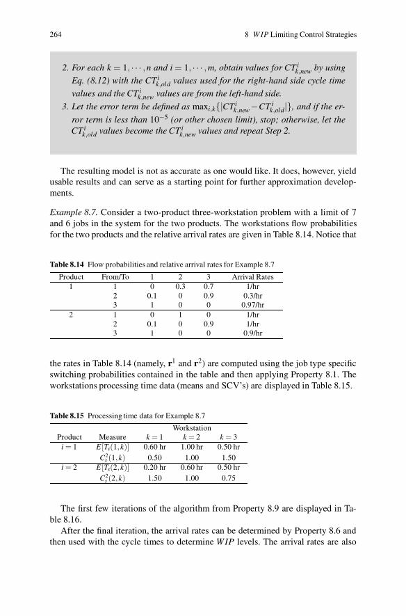
264 8 W IP Limiting Control Strategies
2. For each k = 1, · · · ,n and i = 1, · · · ,m, obtain values for CT ik,new by using
Eq. (8.12) with the CTik,old values used for the right-hand side cycle time
values and the CT ik,new values are from the left-hand side.
3. Let the error term be defined as maxi,k{|CTik,new−CT i
k,old|}, and if the er-
ror term is less than 10−5 (or other chosen limit), stop; otherwise, let theCT i
k,old values become the CT ik,new values and repeat Step 2.
The resulting model is not as accurate as one would like. It does, however, yieldusable results and can serve as a starting point for further approximation develop-ments.
Example 8.7. Consider a two-product three-workstation problem with a limit of 7and 6 jobs in the system for the two products. The workstations flow probabilitiesfor the two products and the relative arrival rates are given in Table 8.14. Notice that
Table 8.14 Flow probabilities and relative arrival rates for Example 8.7
Product From/To 1 2 3 Arrival Rates1 1 0 0.3 0.7 1/hr
2 0.1 0 0.9 0.3/hr3 1 0 0 0.97/hr
2 1 0 1 0 1/hr2 0.1 0 0.9 1/hr3 1 0 0 0.9/hr
the rates in Table 8.14 (namely, r1 and r2) are computed using the job type specificswitching probabilities contained in the table and then applying Property 8.1. Theworkstations processing time data (means and SCV’s) are displayed in Table 8.15.
Table 8.15 Processing time data for Example 8.7
WorkstationProduct Measure k = 1 k = 2 k = 3
i = 1 E [Ts(1,k)] 0.60 hr 1.00 hr 0.50 hrC2
s (1,k) 0.50 1.00 1.50i = 2 E [Ts(2,k)] 0.20 hr 0.60 hr 0.50 hr
C2s (2,k) 1.50 1.00 0.75
The first few iterations of the algorithm from Property 8.9 are displayed in Ta-ble 8.16.
After the final iteration, the arrival rates can be determined by Property 8.6 andthen used with the cycle times to determine WIP levels. The arrival rates are also
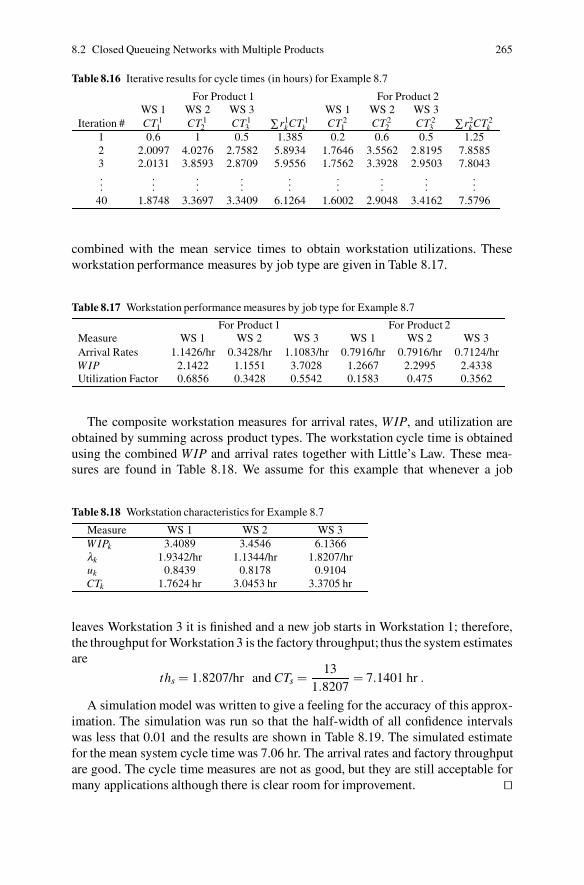
8.2 Closed Queueing Networks with Multiple Products 265
Table 8.16 Iterative results for cycle times (in hours) for Example 8.7
For Product 1 For Product 2WS 1 WS 2 WS 3 WS 1 WS 2 WS 3
Iteration # CT 11 CT 1
2 CT13 ∑r1
kCT 1k CT 2
1 CT22 CT 2
3 ∑r2kCT2
k1 0.6 1 0.5 1.385 0.2 0.6 0.5 1.252 2.0097 4.0276 2.7582 5.8934 1.7646 3.5562 2.8195 7.85853 2.0131 3.8593 2.8709 5.9556 1.7562 3.3928 2.9503 7.8043...
......
......
......
......
40 1.8748 3.3697 3.3409 6.1264 1.6002 2.9048 3.4162 7.5796
combined with the mean service times to obtain workstation utilizations. Theseworkstation performance measures by job type are given in Table 8.17.
Table 8.17 Workstation performance measures by job type for Example 8.7
For Product 1 For Product 2Measure WS 1 WS 2 WS 3 WS 1 WS 2 WS 3Arrival Rates 1.1426/hr 0.3428/hr 1.1083/hr 0.7916/hr 0.7916/hr 0.7124/hrW IP 2.1422 1.1551 3.7028 1.2667 2.2995 2.4338Utilization Factor 0.6856 0.3428 0.5542 0.1583 0.475 0.3562
The composite workstation measures for arrival rates, WIP, and utilization areobtained by summing across product types. The workstation cycle time is obtainedusing the combined WIP and arrival rates together with Little’s Law. These mea-sures are found in Table 8.18. We assume for this example that whenever a job
Table 8.18 Workstation characteristics for Example 8.7
Measure WS 1 WS 2 WS 3W IPk 3.4089 3.4546 6.1366λk 1.9342/hr 1.1344/hr 1.8207/hruk 0.8439 0.8178 0.9104CTk 1.7624 hr 3.0453 hr 3.3705 hr
leaves Workstation 3 it is finished and a new job starts in Workstation 1; therefore,the throughput for Workstation 3 is the factory throughput; thus the system estimatesare
ths = 1.8207/hr and CTs =13
1.8207= 7.1401 hr .
A simulation model was written to give a feeling for the accuracy of this approx-imation. The simulation was run so that the half-width of all confidence intervalswas less that 0.01 and the results are shown in Table 8.19. The simulated estimatefor the mean system cycle time was 7.06 hr. The arrival rates and factory throughputare good. The cycle time measures are not as good, but they are still acceptable formany applications although there is clear room for improvement. ��
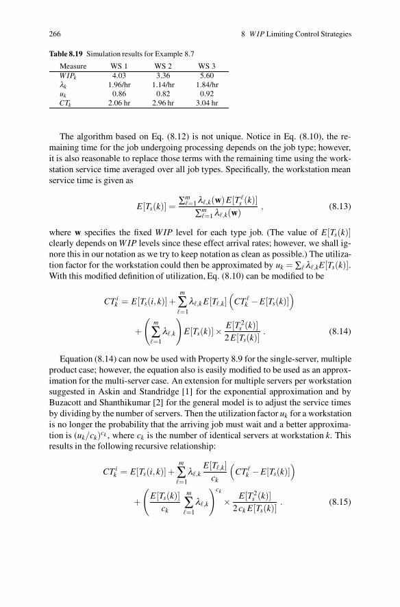
266 8 W IP Limiting Control Strategies
Table 8.19 Simulation results for Example 8.7
Measure WS 1 WS 2 WS 3W IPk 4.03 3.36 5.60λk 1.96/hr 1.14/hr 1.84/hruk 0.86 0.82 0.92CTk 2.06 hr 2.96 hr 3.04 hr
The algorithm based on Eq. (8.12) is not unique. Notice in Eq. (8.10), the re-maining time for the job undergoing processing depends on the job type; however,it is also reasonable to replace those terms with the remaining time using the work-station service time averaged over all job types. Specifically, the workstation meanservice time is given as
E[Ts(k)] =∑m
�=1 λ�,k(w)E[T �s (k)]
∑m�=1 λ�,k(w)
, (8.13)
where w specifies the fixed WIP level for each type job. (The value of E[Ts(k)]clearly depends on W IP levels since these effect arrival rates; however, we shall ig-nore this in our notation as we try to keep notation as clean as possible.) The utiliza-tion factor for the workstation could then be approximated by uk = ∑� λ�,kE[Ts(k)].With this modified definition of utilization, Eq. (8.10) can be modified to be
CT ik = E[Ts(i,k)]+
m
∑�=1
λ�,k E[T�,k](
CT �k −E[Ts(k)]
)
+
(
m
∑�=1
λ�,k
)
E[Ts(k)]×E[T 2
s (k)]2 E[Ts(k)]
. (8.14)
Equation (8.14) can now be used with Property 8.9 for the single-server, multipleproduct case; however, the equation also is easily modified to be used as an approx-imation for the multi-server case. An extension for multiple servers per workstationsuggested in Askin and Standridge [1] for the exponential approximation and byBuzacott and Shanthikumar [2] for the general model is to adjust the service timesby dividing by the number of servers. Then the utilization factor uk for a workstationis no longer the probability that the arriving job must wait and a better approxima-tion is (uk/ck)ck , where ck is the number of identical servers at workstation k. Thisresults in the following recursive relationship:
CT ik = E[Ts(i,k)]+
m
∑�=1
λ�,kE[T�,k]
ck
(
CT �k −E[Ts(k)]
)
+
(
E[Ts(k)]ck
m
∑�=1
λ�,k
)ck
× E[T 2s (k)]
2 ck E[Ts(k)]. (8.15)
8.3 Production and Sequencing Strategies 267
Thus, for the multi-server case, Property 8.9 could be used with Eq. (8.15) toyield approximate cycle times. The iterations are slightly more involved becausethe values for λi,k and E[Ts(k)] must be calculated after each iteration in order toobtain the next estimates for CT i
k , but the extra calculations are not difficult.Although the multi-server approximation based on Eq. (8.15) can give reason-
able results, an iterative method proposed by Marie [9, 10] has been shown to oftengive superior results. Marie’s method uses an aggregation technique that is beyondthe scope of this text; however, the method is worth investigating for those interestedin modeling multi-server networks with non-exponential processing times.
• Suggestion: Do Problem 8.17.
8.3 Production and Sequencing Strategies: A Case Study
In manufacturing systems analysis, the concept of just-in-time manufacturing hasreceived significant interest in recent years. Based on Toyota of Japan’s kanbancontrol concept, the “pull” manufacturing strategy has evolved. This strategy is fun-damentally different from the traditional MPR-type “push” release strategy. Pullversus push production release strategies can have a profound impact on the cycletime for products. This case study will investigate the differences of pull and pushrelease strategies and the impact of scheduling rules on cycle time.
A push-release strategy is one where products are released to the manufacturingsystem based on a schedule. This schedule is usually derived from orders or orderforecasts and the schedule developed based on typical or “standard” production cy-cle times (one such mechanism is the MRP strategy). A pull-release strategy, on theother hand, is one where orders are authorized for release into the shop based onthe completion of processing within the shop. For example, one pull-based controlpolicy is to have a fixed number of parts being manufactured within the shop at anyone time, i.e., a CONWIP control system just analyzed. Hence, when a part is com-pleted and ready for shipping, the next part is released to the shop. In this way, theWIP is controlled and the manufacturing flow times are reduced.
The combination of the job-release strategy (into the system) and the job-sequencing strategy (at a machine center) can have a significant impact on productcycle times. In this case study, these concepts are illustrated and it is shown howto model these schemes for the most complex manufacturing environment - the jobshop. A job shop is a manufacturing system where production steps that requirethe same machinery are processed within the same production area called a ma-chine center. Furthermore, different part types have different routings through theshop and can require multiple processing steps on the same machine. Thus, if thefirst, third and fifth processing steps require the same machine (processing times,of course, can vary by processing step), then the part is routed back to the samemachine center for processing. Due to the re-entrant flow or feedback nature of the

268 8 W IP Limiting Control Strategies
processing routings, this type of manufacturing system is more complex to designand control than the straight-through manufacturing design (called a flow-shop).
In this study, the simulation language used (MOR/DS) was developed by the au-thors [3]; however, the mechanics of simulation model itself are not discussed. Ourconcern is with the results of the study and their implications. The purpose of thissection is two-fold. First, we have always assumed a FIFO (first-in first-out) queue-ing discipline, and this is not always the best possible. Therefore, this case studyshould serve to emphasize that different priority schemes can have a significant ef-fect on cycle times and that a FIFO system is not always preferred. Although thistext presents many mathematical models for manufacturing and production systems,there are still many problems, especially those dealing with sequencing issues, forwhich good mathematical approximations must be developed. Thus the second pur-pose of this section is to illustrate the importance of sequencing and encourage thedevelopment of analysis techniques in this area.
The job-release strategies and the processing sequencing strategies at the work-stations in combination have been the subject of several research studies in recentyears. In this case study, a job shop model is used in conjunction with the strategiesreported in the papers by Wein [13, 14], Harrison and Wein [7], Spearman et al.[12], and Duenyas [5] to illustrate in impact that various control strategies can haveon cycle times. We do not have the space in this textbook to discuss the modeling ofsequencing in coordination with other control strategies, but it is important for thereader to have some understanding of the profound impact that sequencing can haveon factory performance.
8.3.1 Problem Statement
The problem used for illustration purposes is from Wein [14]. This model consistsof three single workstations and three part types to be produced. The part routingsthrough the machine centers and their mean processing times are listed in Table 8.20.Figure 8.3 illustrates the product flow through the facility. All processing times are
Table 8.20 Three-product, three-workstation job shop data from Wein [14]
Product Type Processing Route Mean Times1 3 → 1 → 2 6 min : 4 min : 1 min2 1 → 2 → 3 → 1 → 2 8 min : 6 min : 1 min : 2 min : 7 min3 2 → 3 → 1 → 3 4 min : 9 min : 4 min : 2 min
assumed to be exponentially distributed and the load on each machine center av-erages 89.4% utilization. The three products are to be produced in equal quantitieswith a required total output rate of 8.94 per hour.
Of interest are the effects of a variety of release and sequencing rules on theaverage cycle time for all products. For a workstation with a single machine and a

8.3 Production and Sequencing Strategies 269
Fig. 8.3 Routing diagram forthe problem of Sect. 8.3
1
2
3
in
in
in
out
out
out
fixed job set, sequencing the jobs according to the shortest expected processing time(SEPT ) rule always yields the shortest cycle time; however, it is not necessarilyoptimal for a general job-shop. In this case study, various policies are comparedamong themselves and with a standard push or deterministic release schedule. Thepush variation of the job shop model is given first. The data from Table 8.20 andthe release rates are incorporated into the model. For model specification, there is arelease rule and a sequencing rule for selecting the next job to be processed at themachines. The standard first-in first-out sequencing rule is called the FIFO rule.For job releases into the shop, note that the simulation uses time between releasesand so a deterministic rate of 8.94 per hour results in the time between releases of6.71 minutes. If the three job types are released separately, then the release time is20.13 minutes for each job type since they are to be released in equal numbers. Thisspecific model configuration is denoted as Deter − FIFO (deterministic release,first-in first-out sequencing). Other job sequencing rules order jobs at the machinesin some specified sequence; here the smallest number has the highest priority. Thesequencing rules that will be considered are: SEPT - smallest expected processingtime at the current machine, SRPT - smallest remaining expected processing time atall remaining machines, and W BAL - a workload balance sequencing rule proposedby Harrison and Wein [7], which is essentially SRPT by workstation (includes allremaining visitations to the current workstation).
8.3.2 Push Strategy Model
The general push processing release model is setup to run different sequencing rulesfor the deterministic release policy. The three different polices considered are theSEPT , SRPT , and WBAL rules. The workload-balance sequencing rule (W BAL) as-signs priorities to the jobs at each workstation in the processing sequence accordingto:
Workstation 1: type 2 - step 4, type 3 - step 3, type 1 - step 2, and type 2- step 1;Workstation 2: type 1 - step 3, type 3 - step 1, type 2 - step 5, and type 2 - step 2 ;Workstation 3: type 2 - step 3, type 3 - step 4, type 1 - step 1, and type 3 - step 2.

270 8 W IP Limiting Control Strategies
The workload balance priority sequencing rule (WBAL) gives the highest prior-ity at Workstation i to the job with the smallest remaining expected processing timeto be performed by Workstation i throughout the remainder of the job’s processingsequence. This priority scheme is a variant of the SRPT rule with remaining pro-cessing time being restricted to the workstation in question. To illustrate this priorityscheme, the data from Table 8.20 is used and the sequencing priority for Worksta-tion 1 developed. There are four uses of Workstation 1, these are: product 1-step 2,product 2-steps 1 and 4, and product 3-step 3. The remaining processing times inWorkstation 1 for these four visits are 4, 10, 2, and 4, respectively. Thus, in step4 first priority is given to jobs of product type 2. The tie between product 1-step 2and product 3-step 3 is broken arbitrary in favor of product 3-step 3. Lastly, product2-step 1 is processed. The sequences for the other two workstations are computedsimilarly.
The push-release system is operated by fixing the time between product releasesand staying with that schedule regardless of the number of jobs in the system. Forthis problem, each job type has a desired throughput rate of 3 jobs per hour. Thus, toobtain this throughput rate on a long-term basis, the release rates need be the sameas the desired output rates. Each type of job can either be released at this fixed rate,or a job released to the system at three times that rate and then assigned a type onceactive.
The results for the four sequencing algorithms are displayed in Table 8.21. TheWBAL algorithm yields a mean flow time that is 52% shorter than the worst algo-rithm, SRPT , and 18% better than the next best algorithm, SEPT . In general, thestandard deviations of the flow times follow the same order as the means, exceptthat the FIFO rule yields the lowest, 5.5% lower than the WBAL method.
Table 8.21 Push release policy results for the four job sequencing algorithms with the mean andstandard deviations of the job flow times and throughput rates as given; the results are the averageof 10 replications of length 22,000 with a statistical reset at 2,000
Sequencing Mean Std.Dev. TotalRule Cycle Time Cycle Time Throughput
W BAL 104.3 min 87.7 min 8.88/hrSEPT 127.1 min 130.7 min 8.88/hrFIFO 175.3 min 82.9 min 8.88/hrSRPT 219.3 min 240.6 min 8.82/hr
For push-release control, the work-balance algorithm performs the best of thefour algorithms tested. The best push result, however, can be improved on by limit-ing the total number of jobs allowed in the system (a CONWIP control strategy).
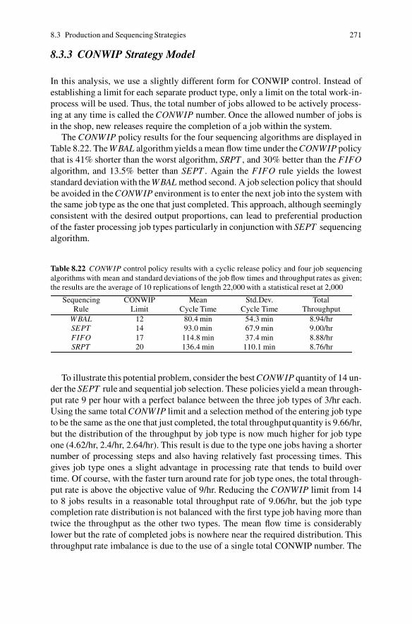
8.3 Production and Sequencing Strategies 271
8.3.3 CONWIP Strategy Model
In this analysis, we use a slightly different form for CONWIP control. Instead ofestablishing a limit for each separate product type, only a limit on the total work-in-process will be used. Thus, the total number of jobs allowed to be actively process-ing at any time is called the CONWIP number. Once the allowed number of jobs isin the shop, new releases require the completion of a job within the system.
The CONWIP policy results for the four sequencing algorithms are displayed inTable 8.22. The W BAL algorithm yields a mean flow time under the CONWIP policythat is 41% shorter than the worst algorithm, SRPT , and 30% better than the FIFOalgorithm, and 13.5% better than SEPT . Again the FIFO rule yields the loweststandard deviation with the W BAL method second. A job selection policy that shouldbe avoided in the CONWIP environment is to enter the next job into the system withthe same job type as the one that just completed. This approach, although seeminglyconsistent with the desired output proportions, can lead to preferential productionof the faster processing job types particularly in conjunction with SEPT sequencingalgorithm.
Table 8.22 CONWIP control policy results with a cyclic release policy and four job sequencingalgorithms with mean and standard deviations of the job flow times and throughput rates as given;the results are the average of 10 replications of length 22,000 with a statistical reset at 2,000
Sequencing CONWIP Mean Std.Dev. TotalRule Limit Cycle Time Cycle Time Throughput
W BAL 12 80.4 min 54.3 min 8.94/hrSEPT 14 93.0 min 67.9 min 9.00/hrFIFO 17 114.8 min 37.4 min 8.88/hrSRPT 20 136.4 min 110.1 min 8.76/hr
To illustrate this potential problem, consider the best CONWIP quantity of 14 un-der the SEPT rule and sequential job selection. These policies yield a mean through-put rate 9 per hour with a perfect balance between the three job types of 3/hr each.Using the same total CONWIP limit and a selection method of the entering job typeto be the same as the one that just completed, the total throughput quantity is 9.66/hr,but the distribution of the throughput by job type is now much higher for job typeone (4.62/hr, 2.4/hr, 2.64/hr). This result is due to the type one jobs having a shorternumber of processing steps and also having relatively fast processing times. Thisgives job type ones a slight advantage in processing rate that tends to build overtime. Of course, with the faster turn around rate for job type ones, the total through-put rate is above the objective value of 9/hr. Reducing the CONWIP limit from 14to 8 jobs results in a reasonable total throughput rate of 9.06/hr, but the job typecompletion rate distribution is not balanced with the first type job having more thantwice the throughput as the other two types. The mean flow time is considerablylower but the rate of completed jobs is nowhere near the required distribution. Thisthroughput rate imbalance is due to the use of a single total CONWIP number. The
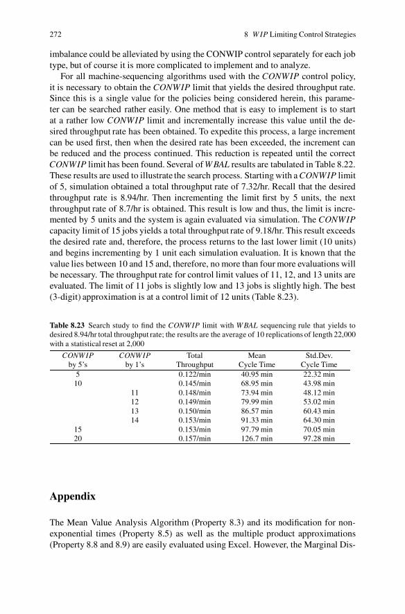
272 8 W IP Limiting Control Strategies
imbalance could be alleviated by using the CONWIP control separately for each jobtype, but of course it is more complicated to implement and to analyze.
For all machine-sequencing algorithms used with the CONWIP control policy,it is necessary to obtain the CONWIP limit that yields the desired throughput rate.Since this is a single value for the policies being considered herein, this parame-ter can be searched rather easily. One method that is easy to implement is to startat a rather low CONWIP limit and incrementally increase this value until the de-sired throughput rate has been obtained. To expedite this process, a large incrementcan be used first, then when the desired rate has been exceeded, the increment canbe reduced and the process continued. This reduction is repeated until the correctCONWIP limit has been found. Several of W BAL results are tabulated in Table 8.22.These results are used to illustrate the search process. Starting with a CONWIP limitof 5, simulation obtained a total throughput rate of 7.32/hr. Recall that the desiredthroughput rate is 8.94/hr. Then incrementing the limit first by 5 units, the nextthroughput rate of 8.7/hr is obtained. This result is low and thus, the limit is incre-mented by 5 units and the system is again evaluated via simulation. The CONWIPcapacity limit of 15 jobs yields a total throughput rate of 9.18/hr. This result exceedsthe desired rate and, therefore, the process returns to the last lower limit (10 units)and begins incrementing by 1 unit each simulation evaluation. It is known that thevalue lies between 10 and 15 and, therefore, no more than four more evaluations willbe necessary. The throughput rate for control limit values of 11, 12, and 13 units areevaluated. The limit of 11 jobs is slightly low and 13 jobs is slightly high. The best(3-digit) approximation is at a control limit of 12 units (Table 8.23).
Table 8.23 Search study to find the CONWIP limit with W BAL sequencing rule that yields todesired 8.94/hr total throughput rate; the results are the average of 10 replications of length 22,000with a statistical reset at 2,000
CONWIP CONWIP Total Mean Std.Dev.by 5’s by 1’s Throughput Cycle Time Cycle Time
5 0.122/min 40.95 min 22.32 min10 0.145/min 68.95 min 43.98 min
11 0.148/min 73.94 min 48.12 min12 0.149/min 79.99 min 53.02 min13 0.150/min 86.57 min 60.43 min14 0.153/min 91.33 min 64.30 min
15 0.153/min 97.79 min 70.05 min20 0.157/min 126.7 min 97.28 min
Appendix
The Mean Value Analysis Algorithm (Property 8.3) and its modification for non-exponential times (Property 8.5) as well as the multiple product approximations(Property 8.8 and 8.9) are easily evaluated using Excel. However, the Marginal Dis-

Problems 273
tribution Analysis Algorithm (Property 8.4) is more complicated and is best handledin Excel with VBA as is the algorithm of Property 8.7. In this appendix, we give theExcel formula needed for the Mean Value Analysis Algorithm and leave the exten-sions to the reader. The material in the Appendix of Chap. 3 can be used to find therelative arrival rates (Property 8.1) of a network. Given the vector r, the followingcan be used to obtain the cycle times for the network of Example 8.2.
The initial data of the problem is established by the following.
A B C D E1 E[Ts-1] E[Ts-2] E[Ts-3]2 0.2 0.5 0.53 r-1 r-2 r-34 1 1 0.9
We skip a row and then setup for the algorithm.
A B C D E6 w CT-1 CT-2 CT-3 Sum7 1 =B2 =C2 =D2
In Cell A8, type =A7+1 and the copy Cell A8 down to Cell A20. In Cell E7, type
=SUMPRODUCT(B7:D7,$B$4:$D$4)
and copy Cell E7 down through Cell E20. Finally, the main iterative step is typedinto Cell B8 as
=B$2+B$2*$A7*B$4*B7/$E7
and then Cell B8 is copied to the right through Cell D8 and then B8 is copied down tothrough Cell D20. It is important when typing the various formulas that care is takento type the dollar signs ($) exactly as shown since at times the row indicator mustbe an absolute address and sometimes the column indicator must be an absoluteaddress. The resulting spreadsheet should give the Mean Value Algorithm througha CONWIP level of 14.
Problems
8.1. Find the relative flow rates for the network displayed in Fig. 8.4.
8.2. Find the relative flow rates for the network displayed in Fig. 8.6.
8.3. Re-consider the Example 8.2 and find the workstation and system performancemeasures for a CONWIP level of(a) 7 jobs, and(b) 10 jobs.
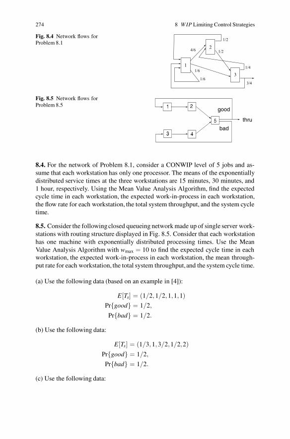
274 8 W IP Limiting Control Strategies
Fig. 8.4 Network flows forProblem 8.1
1
2
3
4/6
1/6
1/6
1/2
1/2
1/4
3/4
Fig. 8.5 Network flows forProblem 8.5
thru
good
bad
8.4. For the network of Problem 8.1, consider a CONWIP level of 5 jobs and as-sume that each workstation has only one processor. The means of the exponentiallydistributed service times at the three workstations are 15 minutes, 30 minutes, and1 hour, respectively. Using the Mean Value Analysis Algorithm, find the expectedcycle time in each workstation, the expected work-in-process in each workstation,the flow rate for each workstation, the total system throughput, and the system cycletime.
8.5. Consider the following closed queueing network made up of single server work-stations with routing structure displayed in Fig. 8.5. Consider that each workstationhas one machine with exponentially distributed processing times. Use the MeanValue Analysis Algorithm with wmax = 10 to find the expected cycle time in eachworkstation, the expected work-in-process in each workstation, the mean through-put rate for each workstation, the total system throughput,and the system cycle time.
(a) Use the following data (based on an example in [4]):
E[Ts] = (1/2,1/2,1,1,1)Pr{good} = 1/2,
Pr{bad} = 1/2.
(b) Use the following data:
E[Ts] = (1/3,1,3/2,1/2,2)Pr{good} = 1/2,
Pr{bad} = 1/2.
(c) Use the following data:
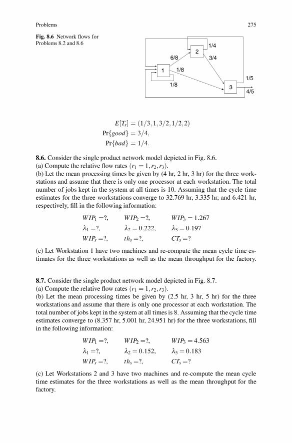
Problems 275
Fig. 8.6 Network flows forProblems 8.2 and 8.6
1
2
3
6/8
1/8
1/8
1/4
3/4
4/5
1/5
E[Ts] = (1/3,1,3/2,1/2,2)Pr{good} = 3/4,
Pr{bad} = 1/4.
8.6. Consider the single product network model depicted in Fig. 8.6.(a) Compute the relative flow rates (r1 = 1, r2, r3).(b) Let the mean processing times be given by (4 hr, 2 hr, 3 hr) for the three work-stations and assume that there is only one processor at each workstation. The totalnumber of jobs kept in the system at all times is 10. Assuming that the cycle timeestimates for the three workstations converge to 32.769 hr, 3.335 hr, and 6.421 hr,respectively, fill in the following information:
W IP1 =?, W IP2 =?, WIP3 = 1.267
λ1 =?, λ2 = 0.222, λ3 = 0.197
W IPs =?, ths =?, CTs =?
(c) Let Workstation 1 have two machines and re-compute the mean cycle time es-timates for the three workstations as well as the mean throughput for the factory.
8.7. Consider the single product network model depicted in Fig. 8.7.(a) Compute the relative flow rates (r1 = 1, r2, r3).(b) Let the mean processing times be given by (2.5 hr, 3 hr, 5 hr) for the threeworkstations and assume that there is only one processor at each workstation. Thetotal number of jobs kept in the system at all times is 8. Assuming that the cycle timeestimates converge to (8.357 hr, 5.001 hr, 24.951 hr) for the three workstations, fillin the following information:
W IP1 =?, W IP2 =?, WIP3 = 4.563
λ1 =?, λ2 = 0.152, λ3 = 0.183
W IPs =?, ths =?, CTs =?
(c) Let Workstations 2 and 3 have two machines and re-compute the mean cycletime estimates for the three workstations as well as the mean throughput for thefactory.
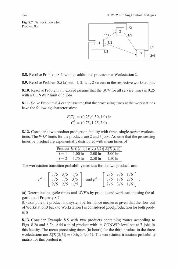
276 8 WIP Limiting Control Strategies
Fig. 8.7 Network flows forProblem 8.7
1
2
3
1/3
1/3
1/3
1/2
1/2
3/4
1/4
8.8. Resolve Problem 8.4, with an additional processor at Workstation 2.
8.9. Resolve Problem 8.5 (a) with 1, 2, 1, 1, 2 servers in the respective workstations.
8.10. Resolve Problem 8.3 except assume that the SCV for all service times is 0.25with a CONWIP limit of 5 jobs.
8.11. Solve Problem8.4 except assume that the processing times at the workstationshave the following characteristics:
E[Ts] = (0.25,0.50,1.0) hrC2s = (0.75,1.25,2.0) .
8.12. Consider a two product production facility with three, single-server worksta-tions. TheWIP limits for the products are 2 and 3 jobs. Assume that the processingtimes by product are exponentially distributed with mean times of
Product E[Ts(i,1)] E[Ts(i,2)] E[Ts(i,3)]i = 1 1.00 hr 2.00 hr 3.00 hri = 2 1.75 hr 2.50 hr 1.50 hr
The workstation transition probabilitymatrices for the two products are:
P1 =
⎡⎣ 1/5 3/5 1/51/5 1/5 3/52/5 2/5 1/5
⎤⎦ and p2 =
⎡⎣ 2/6 3/6 1/63/6 1/6 2/62/6 3/6 1/6
⎤⎦ .
(a) Determine the cycle times and WIP’s by product and workstation using the al-gorithm of Property 8.7.(b) Compute the product and system performance measures given that the flow outofWorkstation3 back toWorkstation1 is consideredgood production for both prod-ucts.
8.13. Consider Example 8.5 with two products containing routes according toFigs. 8.2a and 8.2b. Add a third product with its CONWIP level set at 7 jobs inthis facility. The mean processing times (in hours) for the third product in the threeworkstations are E[Ts(3,k)] = (0.6,0.4,0.5).The workstation transition probabilitymatrix for this product is
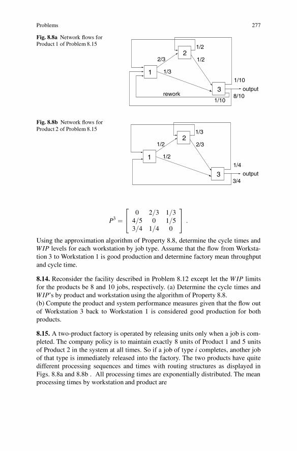
Problems 277
Fig. 8.8a Network flows forProduct 1 of Problem 8.15
1
2
3
2/3
1/3
1/2
1/2
8/10
1/10
rework1/10
output
Fig. 8.8b Network flows forProduct 2 of Problem 8.15
1
2
3
1/2
1/2
1/3
2/3
3/4
1/4
output
P3 =
⎡
⎣
0 2/3 1/34/5 0 1/53/4 1/4 0
⎤
⎦ .
Using the approximation algorithm of Property 8.8, determine the cycle times andWIP levels for each workstation by job type. Assume that the flow from Worksta-tion 3 to Workstation 1 is good production and determine factory mean throughputand cycle time.
8.14. Reconsider the facility described in Problem 8.12 except let the W IP limitsfor the products be 8 and 10 jobs, respectively. (a) Determine the cycle times andWIP’s by product and workstation using the algorithm of Property 8.8.(b) Compute the product and system performance measures given that the flow outof Workstation 3 back to Workstation 1 is considered good production for bothproducts.
8.15. A two-product factory is operated by releasing units only when a job is com-pleted. The company policy is to maintain exactly 8 units of Product 1 and 5 unitsof Product 2 in the system at all times. So if a job of type i completes, another jobof that type is immediately released into the factory. The two products have quitedifferent processing sequences and times with routing structures as displayed inFigs. 8.8a and 8.8b . All processing times are exponentially distributed. The meanprocessing times by workstation and product are
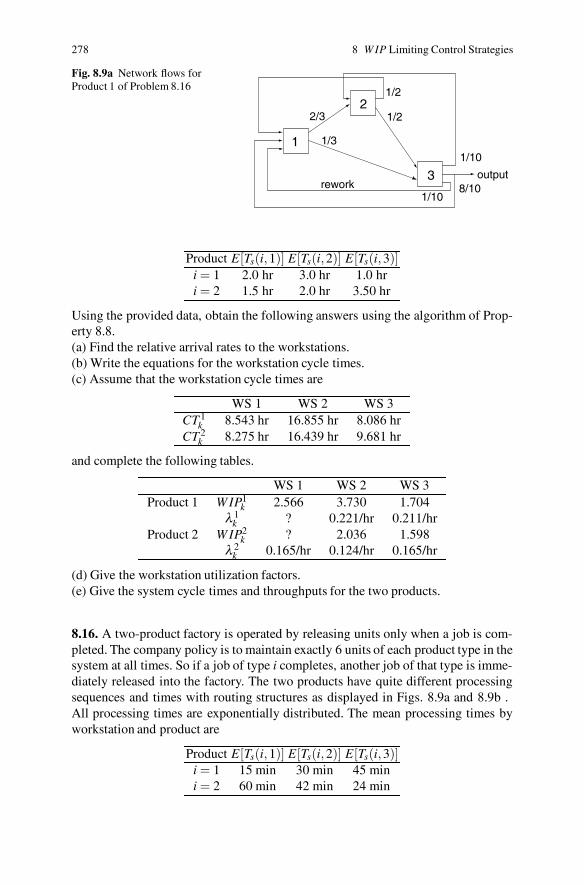
278 8 W IP Limiting Control Strategies
Fig. 8.9a Network flows forProduct 1 of Problem 8.16
1
2
3
2/3
1/3
1/2
1/2
8/10
1/10
rework1/10
output
Product E[Ts(i,1)] E[Ts(i,2)] E[Ts(i,3)]i = 1 2.0 hr 3.0 hr 1.0 hri = 2 1.5 hr 2.0 hr 3.50 hr
Using the provided data, obtain the following answers using the algorithm of Prop-erty 8.8.(a) Find the relative arrival rates to the workstations.(b) Write the equations for the workstation cycle times.(c) Assume that the workstation cycle times are
WS 1 WS 2 WS 3CT 1
k 8.543 hr 16.855 hr 8.086 hrCT 2
k 8.275 hr 16.439 hr 9.681 hr
and complete the following tables.
WS 1 WS 2 WS 3Product 1 W IP1
k 2.566 3.730 1.704λ 1
k ? 0.221/hr 0.211/hrProduct 2 W IP2
k ? 2.036 1.598λ 2
k 0.165/hr 0.124/hr 0.165/hr
(d) Give the workstation utilization factors.(e) Give the system cycle times and throughputs for the two products.
8.16. A two-product factory is operated by releasing units only when a job is com-pleted. The company policy is to maintain exactly 6 units of each product type in thesystem at all times. So if a job of type i completes, another job of that type is imme-diately released into the factory. The two products have quite different processingsequences and times with routing structures as displayed in Figs. 8.9a and 8.9b .All processing times are exponentially distributed. The mean processing times byworkstation and product are
Product E[Ts(i,1)] E[Ts(i,2)] E[Ts(i,3)]i = 1 15 min 30 min 45 mini = 2 60 min 42 min 24 min
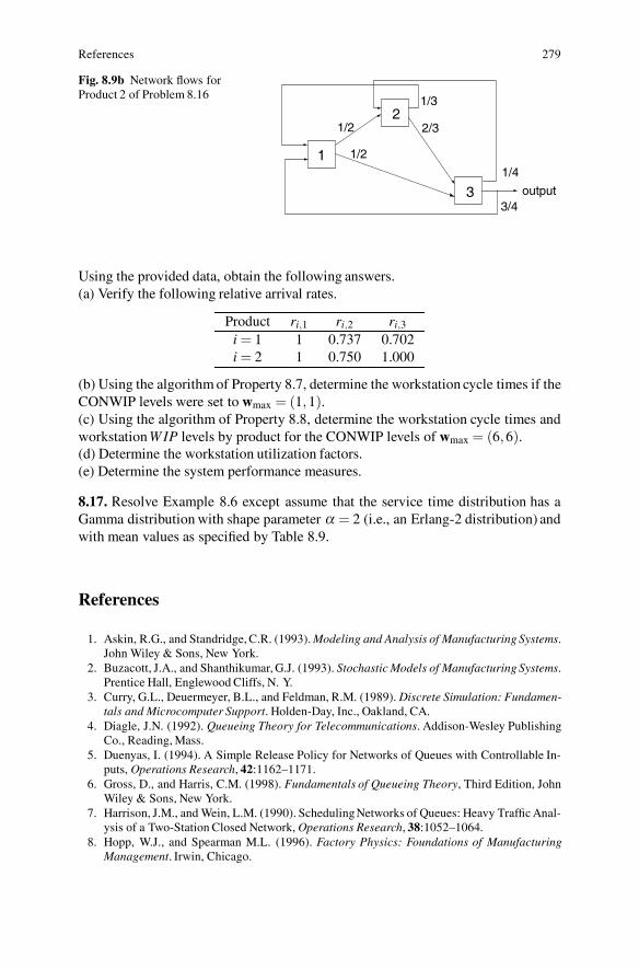
References 279
Fig. 8.9b Network flows forProduct 2 of Problem 8.16
1
2
3
1/2
1/2
1/3
2/3
3/4
1/4
output
Using the provided data, obtain the following answers.(a) Verify the following relative arrival rates.
Product ri,1 ri,2 ri,3
i = 1 1 0.737 0.702i = 2 1 0.750 1.000
(b) Using the algorithm of Property 8.7, determine the workstation cycle times if theCONWIP levels were set to wmax = (1,1).(c) Using the algorithm of Property 8.8, determine the workstation cycle times andworkstation W IP levels by product for the CONWIP levels of wmax = (6,6).(d) Determine the workstation utilization factors.(e) Determine the system performance measures.
8.17. Resolve Example 8.6 except assume that the service time distribution has aGamma distribution with shape parameter α = 2 (i.e., an Erlang-2 distribution) andwith mean values as specified by Table 8.9.
References
1. Askin, R.G., and Standridge, C.R. (1993). Modeling and Analysis of Manufacturing Systems.John Wiley & Sons, New York.
2. Buzacott, J.A., and Shanthikumar, G.J. (1993). Stochastic Models of Manufacturing Systems.Prentice Hall, Englewood Cliffs, N. Y.
3. Curry, G.L., Deuermeyer, B.L., and Feldman, R.M. (1989). Discrete Simulation: Fundamen-tals and Microcomputer Support. Holden-Day, Inc., Oakland, CA.
4. Diagle, J.N. (1992). Queueing Theory for Telecommunications. Addison-Wesley PublishingCo., Reading, Mass.
5. Duenyas, I. (1994). A Simple Release Policy for Networks of Queues with Controllable In-puts, Operations Research, 42:1162–1171.
6. Gross, D., and Harris, C.M. (1998). Fundamentals of Queueing Theory, Third Edition, JohnWiley & Sons, New York.
7. Harrison, J.M., and Wein, L.M. (1990). SchedulingNetworks of Queues: Heavy Traffic Anal-ysis of a Two-Station Closed Network, Operations Research, 38:1052–1064.
8. Hopp, W.J., and Spearman M.L. (1996). Factory Physics: Foundations of ManufacturingManagement. Irwin, Chicago.
280 8 W IP Limiting Control Strategies
9. Marie, R.A. (1979). An Approximate Analytical Method for General Queueing Networks.IEEE Transactions on Software Engineering, 5:530–538.
10. Marie, R.A. (1980). Calculating Equilibrium Probabilities for λ(n)/Ck/1/N Queues. Perfor-mance Evaluation Review, 9:117–125.
11. Reiser, M., and Lavenberg, S.S. (1980). Mean-Value Analysis of Closed Multichain QueuingNetworks. J. Association for Computing Machinery, 27:313–322.
12. Spearman, M.L., Woodruff, D.L., and Hopp, W.J. (1990). CONWIP: A Pull Alternative toKanban, International Journal of Production Research, 28:879–894.
13. Wein, L.M. (1990). SchedulingNetworks of Queues: Heavy TrafficAnalysis of a Two-StationClosed Network with Controllable Inputs, Operations Research, 38:1065–1078.
14. Wein, L.M. (1992). SchedulingNetworks of Queues: Heavy Traffic Analysis of a MultistationNetwork with Controllable Inputs, Operations Research, 40:S312–S344.
Chapter 9Serial Limited Buffer Models
Limited buffer capacity models can be used for the mathematical representations ofa form of kanban control. There are two aspects of limited buffer systems studiedin this chapter. First an approach for developing an analytical approximation modelfor serial flow systems is developed. Then the issue of how these buffer values canbe set to yield an optimal system configuration is addressed.
The systems considered here consist of a set of workstations that have limits onthe number of work-in-process units allowed to wait at each of the single-serverprocessing stations. For serial systems, these workstations are connected in a serialconfiguration so that jobs flow from the first to the second workstation only, andthen from the second to the third workstation, etc., until they exit the facility. Thus,all jobs have the same routing sequence. The workstations have a set number ofjobs that are allowed into the workstation simultaneously and these limits need notbe identical. Let wk represent the work-in-process capacity limitation for Worksta-tion k. This is the total number of jobs allowed in the workstation including the jobbeing processed. Only single-server machines in each workstation are considered;the complexities of multiple servers in a limited-buffer capacity model is beyond thescope of this analysis. (Thus, Workstation k will process jobs on Machine k so theterms Workstation k and Machine k will be used interchangeably.)
There are several methods of operating a W IP-limiting control strategy. The ma-jor policy is that a job may not proceed to the next workstation until a space becomesavailable in that workstation. However, there are several ways the workstation canoperate. The concept of process blocking after job completion is generally used inanalytical models. That is, when a job is finished, it may not be removed from themachine until space is available in the next workstation for this job. This effectivelyblocks the machine from processing other jobs in its queue and is called blockingafter service. Another variation is blocking before service, that is the machine can-not process the job until it has the authorization to move to the next workstation. Acontrol procedure frequently used in practice processes queued jobs in the worksta-tion until they all have been processed and the machine is forced to be idle due tothe lack of unfinished inventory. In this chapter, only the blocking after processingstrategy is implemented for modeling purposes. This strategy allows for the imme-
281
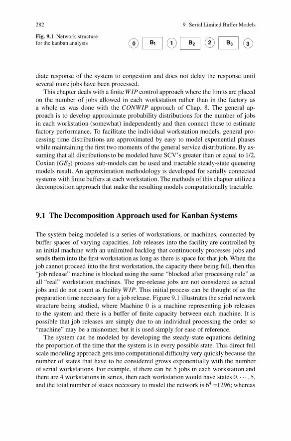
282 9 Serial Limited Buffer Models
Fig. 9.1 Network structurefor the kanban analysis 0 1 2 3B B B1 2 3
diate response of the system to congestion and does not delay the response untilseveral more jobs have been processed.
This chapter deals with a finite W IP control approach where the limits are placedon the number of jobs allowed in each workstation rather than in the factory asa whole as was done with the CONWIP approach of Chap. 8. The general ap-proach is to develop approximate probability distributions for the number of jobsin each workstation (somewhat) independently and then connect these to estimatefactory performance. To facilitate the individual workstation models, general pro-cessing time distributions are approximated by easy to model exponential phaseswhile maintaining the first two moments of the general service distributions. By as-suming that all distributions to be modeled have SCV’s greater than or equal to 1/2,Coxian (GE2) process sub-models can be used and tractable steady-state queueingmodels result. An approximation methodology is developed for serially connectedsystems with finite buffers at each workstation. The methods of this chapter utilize adecomposition approach that make the resulting models computationally tractable.
9.1 The Decomposition Approach used for Kanban Systems
The system being modeled is a series of workstations, or machines, connected bybuffer spaces of varying capacities. Job releases into the facility are controlled byan initial machine with an unlimited backlog that continuously processes jobs andsends them into the first workstation as long as there is space for that job. When thejob cannot proceed into the first workstation, the capacity there being full, then this“job release” machine is blocked using the same “blocked after processing rule” asall “real” workstation machines. The pre-release jobs are not considered as actualjobs and do not count as facility WIP. This initial process can be thought of as thepreparation time necessary for a job release. Figure 9.1 illustrates the serial networkstructure being studied, where Machine 0 is a machine representing job releasesto the system and there is a buffer of finite capacity between each machine. It ispossible that job releases are simply due to an individual processing the order so“machine” may be a misnomer, but it is used simply for ease of reference.
The system can be modeled by developing the steady-state equations definingthe proportion of the time that the system is in every possible state. This direct fullscale modeling approach gets into computational difficulty very quickly because thenumber of states that have to be considered grows exponentially with the numberof serial workstations. For example, if there can be 5 jobs in each workstation andthere are 4 workstations in series, then each workstation would have states 0, · · · ,5,and the total number of states necessary to model the network is 64 =1296; whereas
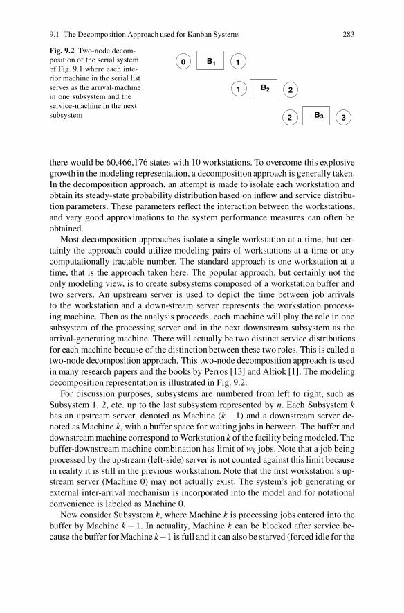
9.1 The Decomposition Approach used for Kanban Systems 283
Fig. 9.2 Two-node decom-position of the serial systemof Fig. 9.1 where each inte-rior machine in the serial listserves as the arrival-machinein one subsystem and theservice-machine in the nextsubsystem
B
B
B
1
2
3
0 1
1 2
2 3
there would be 60,466,176 states with 10 workstations. To overcome this explosivegrowth in the modeling representation, a decomposition approach is generally taken.In the decomposition approach, an attempt is made to isolate each workstation andobtain its steady-state probability distribution based on inflow and service distribu-tion parameters. These parameters reflect the interaction between the workstations,and very good approximations to the system performance measures can often beobtained.
Most decomposition approaches isolate a single workstation at a time, but cer-tainly the approach could utilize modeling pairs of workstations at a time or anycomputationally tractable number. The standard approach is one workstation at atime, that is the approach taken here. The popular approach, but certainly not theonly modeling view, is to create subsystems composed of a workstation buffer andtwo servers. An upstream server is used to depict the time between job arrivalsto the workstation and a down-stream server represents the workstation process-ing machine. Then as the analysis proceeds, each machine will play the role in onesubsystem of the processing server and in the next downstream subsystem as thearrival-generating machine. There will actually be two distinct service distributionsfor each machine because of the distinction between these two roles. This is called atwo-node decomposition approach. This two-node decomposition approach is usedin many research papers and the books by Perros [13] and Altiok [1]. The modelingdecomposition representation is illustrated in Fig. 9.2.
For discussion purposes, subsystems are numbered from left to right, such asSubsystem 1, 2, etc. up to the last subsystem represented by n. Each Subsystem khas an upstream server, denoted as Machine (k− 1) and a downstream server de-noted as Machine k, with a buffer space for waiting jobs in between. The buffer anddownstream machine correspond to Workstation k of the facility being modeled. Thebuffer-downstream machine combination has limit of wk jobs. Note that a job beingprocessed by the upstream (left-side) server is not counted against this limit becausein reality it is still in the previous workstation. Note that the first workstation’s up-stream server (Machine 0) may not actually exist. The system’s job generating orexternal inter-arrival mechanism is incorporated into the model and for notationalconvenience is labeled as Machine 0.
Now consider Subsystem k, where Machine k is processing jobs entered into thebuffer by Machine k− 1. In actuality, Machine k can be blocked after service be-cause the buffer for Machine k+1 is full and it can also be starved (forced idle for the

284 9 Serial Limited Buffer Models
lack of jobs) because of upstream workstation behavior. The blocking of Machine kcannot be mimicked in the decomposition based on knowledge of the subsystem’sstate-probability distribution because of the disconnection between workstations inthe decomposition methodology. Thus, to account for this potential delay, an ap-propriate delay as part of the job processing time is incorporated. Therefore, in thedecomposition structure, the processing time at a server will be longer than the nom-inal processing time. This time will incorporate the probability of blocking due tothe next subsystem being full and an appropriate delay time for completing process-ing at this server to relieve the blockage. Note that the downstream server in turncould be blocked by its downstream subsystem being full and also be forced to waitfor a process completion there, and so forth all the way downstream until the lastserver has been reached. The last server in the serial system can never be blocked. Itis assumed that completed jobs are immediately transported to shipping, or storage,etc., and hence leave the system immediately.
The blocking of an upstream server in a subsystem can be properly accountedfor from the known probability distribution for the subsystem states. Hence, the up-stream server’s processing time does not have to account for downstream blocking.It will, however, be left periodically without a job to process (this situation is re-ferred to as the machine being starved). The additional delay until a job becomesavailable for the upstream server to process must be incorporated into the upstreammachine’s processing time. This delay occurs with a known probability based on theupstream subsystem’s steady-state probability distribution and the associated delaytime is the remaining processing time for the current job on that machine. However,in turn, this workstation could also be starved and forced to wait on its upstreamserver, and so forth all the way back to the job generating Machine 0. This firstmachine can never be starved.
This discussion hopefully has instilled a feeling for the differences in the twoservice times for a given machine when it is playing the role of either the upstreamor the downstream server in the decomposition procedure. One of the main tasks inthe implementation of this decomposition procedure is the estimation of these twodistinct service distributions for each machine. These processes are discussed in thenext section.
9.2 Modeling The Two-Node Subsystem
The first aspect of modeling each subsystem is to describe each server within thetwo-machine subsystem. Initially, the machines will be modeled as exponential pro-cesses, then modeled by a mixture of generalized Erlangs with two or three phases(described in the next subsection), and finally approximated by a two-phase gen-eralized Erlang. Once the machines are described, a state space will be developedusing the general approach of Sect. 3.6.
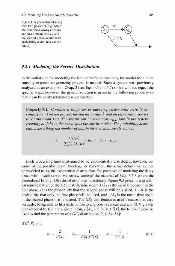
9.2 Modeling The Two-Node Subsystem 285
Fig. 9.3 A generalized Erlangwith two phases (GE2), wherethe first phase always occursand has a mean rate λ1 andthe second phase occurs withprobability α and has a meanrate λ2
(1−α)
λ2α
λ1
9.2.1 Modeling the Service Distribution
In the initial step for modeling the limited buffer subsystems, the model for a finitecapacity exponential queueing process is needed. Such a system was previouslyanalyzed as an example in Chap. 3 (see Eqs. 3.5 and 3.7) so we will not repeat thespecific steps; however, the general solution is given in the following property sothat it can be easily referenced when needed.
Property 9.1. Consider a single-server queueing system with arrivals ac-cording to a Poisson process having mean rate λ and an exponential servicetime with mean 1/μ. The system can have at most wmax jobs in the system,counting all jobs in the queue plus the one in service. The probability distri-bution describing the number of jobs in the system in steady-state is
pi =(λ/μ)i
∑wmaxj=0 (λ/μ) j for i = 0, · · · ,wmax .
Each processing time is assumed to be exponentially distributed; however, be-cause of the possibilities of blockage or starvation, the actual delay time cannotbe modeled using the exponential distribution. For purposes of modeling the delaytimes within each server, we review some of the material of Sect. 3.6.3 where thegeneralized Erlang (GE) distribution was introduced. Figure 9.3 presents a graphi-cal representation of the GE2 distribution, where 1/λ1 is the mean time spent in thefirst phase, α is the probability that the second phase will be visited, 1−α is theprobability that only the first phase will be used, and 1/λ2 is the mean time spentin the second phase if it is visited. The GE2 distribution is used because it is veryversatile, being able to fit a distribution to any positive mean and any SCV greaterthan or equal to 1/2. For a given mean, E[X ], and SCV, C2[X ], the following can beused to find the parameters of a GE2 distribution [2, p. 54–56]:
If C2[X ] > 1,
λ1 =2
E[X ], λ2 =
1E[X ]C2[X ]
, α =1
2C2[X ]; (9.1)
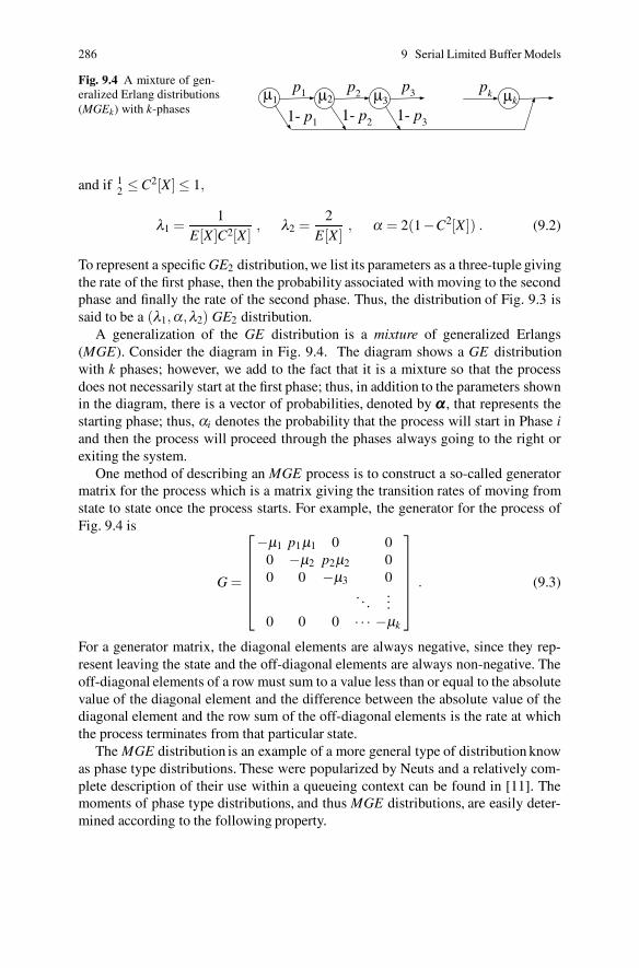
286 9 Serial Limited Buffer Models
Fig. 9.4 A mixture of gen-eralized Erlang distributions(MGEk) with k-phases
p1 p2 p3 pkμ1 μ2 μ3 μk
1- p1 1- p2 1- p3
and if 12 ≤C2[X ]≤ 1,
λ1 =1
E[X ]C2[X ], λ2 =
2E[X ]
, α = 2(1−C2[X ]) . (9.2)
To represent a specific GE2 distribution, we list its parameters as a three-tuple givingthe rate of the first phase, then the probability associated with moving to the secondphase and finally the rate of the second phase. Thus, the distribution of Fig. 9.3 issaid to be a (λ1,α,λ2) GE2 distribution.
A generalization of the GE distribution is a mixture of generalized Erlangs(MGE). Consider the diagram in Fig. 9.4. The diagram shows a GE distributionwith k phases; however, we add to the fact that it is a mixture so that the processdoes not necessarily start at the first phase; thus, in addition to the parameters shownin the diagram, there is a vector of probabilities, denoted by ααα , that represents thestarting phase; thus, αi denotes the probability that the process will start in Phase iand then the process will proceed through the phases always going to the right orexiting the system.
One method of describing an MGE process is to construct a so-called generatormatrix for the process which is a matrix giving the transition rates of moving fromstate to state once the process starts. For example, the generator for the process ofFig. 9.4 is
G =
⎡
⎢
⎢
⎢
⎢
⎢
⎣
−μ1 p1μ1 0 00 −μ2 p2μ2 00 0 −μ3 0
. . ....
0 0 0 · · · −μk
⎤
⎥
⎥
⎥
⎥
⎥
⎦
. (9.3)
For a generator matrix, the diagonal elements are always negative, since they rep-resent leaving the state and the off-diagonal elements are always non-negative. Theoff-diagonal elements of a row must sum to a value less than or equal to the absolutevalue of the diagonal element and the difference between the absolute value of thediagonal element and the row sum of the off-diagonal elements is the rate at whichthe process terminates from that particular state.
The MGE distribution is an example of a more general type of distribution knowas phase type distributions. These were popularized by Neuts and a relatively com-plete description of their use within a queueing context can be found in [11]. Themoments of phase type distributions, and thus MGE distributions, are easily deter-mined according to the following property.

9.2 Modeling The Two-Node Subsystem 287
Fig. 9.5 The MGE3 servicetime process for Example 9.1 2 3 4
0.10 0.15
0.90 0.85
Property 9.2. The moments for a random variable, T , having a phase-typedistribution with generator G and initial probability vector ααα are given by
E[T ] = −ααα G−1 1
E[T 2] = 2ααα G−2 1
E[T 3] = −6ααα G−3 1 ,
where ααα is a row vector, 1 is a column vector of all ones, and G−n = (G−1)n.
Example 9.1. Assume that the processing time for a workstation is described by anMGE3 process where the mean sojourn times for the three phases are 1/2 hr, 1/3 hr,and 1/4 hr, respectively. Furthermore, there is a 90% chance that if the service startsin the first phase it will be finished after the first phase, and an 85% chance thatif the process makes it to the second phase, that it will be finished after that phase(Fig. 9.5). In addition, there is a 90% probability that the process will start in thefirst phase and there is a 10% that it will start in the second phase. For this process,the generator matrix is
G =
⎡
⎣
−2 0.2 00 −3 0.450 0 −4
⎤
⎦ .
and ααα = (0.9,0.1,0). To obtain the moments for the process, the inverse of thegenerator is needed, and this is
G−1 =
⎡
⎣
−0.5 −0.03333 −0.003750 −0.03333 −0.003750 0 −0.25
⎤
⎦ .
Property 9.2 yields a mean of E[T ] = 0.5205 hr and a second moment of E[T 2] =0.5339 hr2; thus, the SCV is C2[T ] = 0.971.
To approximate the MGE3 distribution with a GE2 distribution, Eq. (9.2) is usedto fit the moments. This yields a (1.9792, 0.0586, 3.8425) GE2 distribution. In otherwords, the approximation always starts in the first phase having a mean rate of1.9792/hr, then with probability 5.86% it will enter a second phase having a rateof 3.8425/hr and with probability 94.14% it will finish after the first phase. ��
• Suggestion: Do Problems 9.1–9.3.
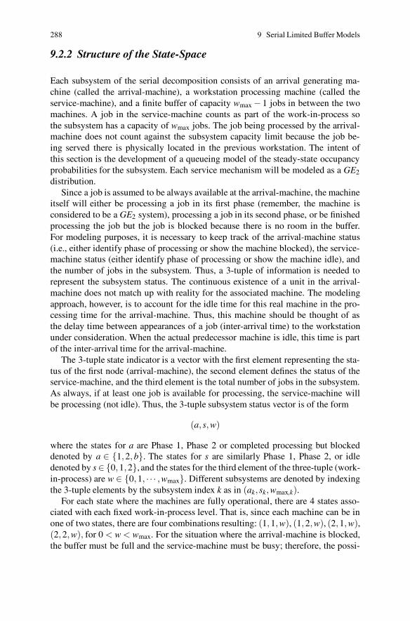
288 9 Serial Limited Buffer Models
9.2.2 Structure of the State-Space
Each subsystem of the serial decomposition consists of an arrival generating ma-chine (called the arrival-machine), a workstation processing machine (called theservice-machine), and a finite buffer of capacity wmax − 1 jobs in between the twomachines. A job in the service-machine counts as part of the work-in-process sothe subsystem has a capacity of wmax jobs. The job being processed by the arrival-machine does not count against the subsystem capacity limit because the job be-ing served there is physically located in the previous workstation. The intent ofthis section is the development of a queueing model of the steady-state occupancyprobabilities for the subsystem. Each service mechanism will be modeled as a GE2
distribution.Since a job is assumed to be always available at the arrival-machine, the machine
itself will either be processing a job in its first phase (remember, the machine isconsidered to be a GE2 system), processing a job in its second phase, or be finishedprocessing the job but the job is blocked because there is no room in the buffer.For modeling purposes, it is necessary to keep track of the arrival-machine status(i.e., either identify phase of processing or show the machine blocked), the service-machine status (either identify phase of processing or show the machine idle), andthe number of jobs in the subsystem. Thus, a 3-tuple of information is needed torepresent the subsystem status. The continuous existence of a unit in the arrival-machine does not match up with reality for the associated machine. The modelingapproach, however, is to account for the idle time for this real machine in the pro-cessing time for the arrival-machine. Thus, this machine should be thought of asthe delay time between appearances of a job (inter-arrival time) to the workstationunder consideration. When the actual predecessor machine is idle, this time is partof the inter-arrival time for the arrival-machine.
The 3-tuple state indicator is a vector with the first element representing the sta-tus of the first node (arrival-machine), the second element defines the status of theservice-machine, and the third element is the total number of jobs in the subsystem.As always, if at least one job is available for processing, the service-machine willbe processing (not idle). Thus, the 3-tuple subsystem status vector is of the form
(a, s,w)
where the states for a are Phase 1, Phase 2 or completed processing but blockeddenoted by a ∈ {1,2,b}. The states for s are similarly Phase 1, Phase 2, or idledenoted by s ∈ {0,1,2}, and the states for the third element of the three-tuple (work-in-process) are w ∈ {0,1, · · · ,wmax}. Different subsystems are denoted by indexingthe 3-tuple elements by the subsystem index k as in (ak, sk,wmax,k).
For each state where the machines are fully operational, there are 4 states asso-ciated with each fixed work-in-process level. That is, since each machine can be inone of two states, there are four combinations resulting: (1,1,w), (1,2,w), (2,1,w),(2,2,w), for 0 < w < wmax. For the situation where the arrival-machine is blocked,the buffer must be full and the service-machine must be busy; therefore, the possi-
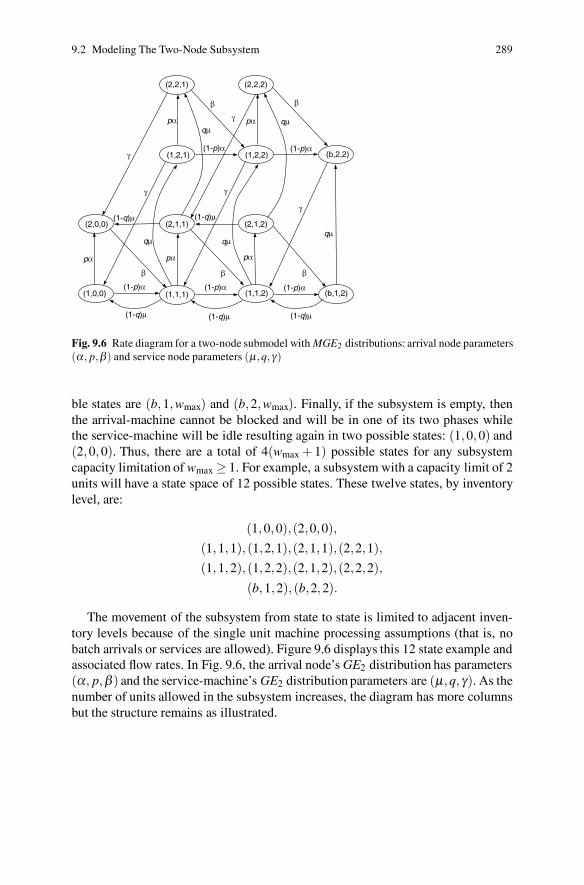
9.2 Modeling The Two-Node Subsystem 289
(1,0,0) (1,1,1) (1,1,2) (b,1,2)
(2,0,0) (2,1,1) (2,1,2)
(1,2,1) (1,2,2) (b,2,2)
(2,2,1) (2,2,2)
γ
γ
γ
γ
β β β
β β
qμqμ
qμ qμ
(1-q)μ
(1-q)μ (1-q)μ (1-q)μ
(1-q)μ
pα pα pα
pα pα
(1-p)α(1-p)α
(1-p)α(1-p)α(1-p)α
γ
qμ
Fig. 9.6 Rate diagram for a two-node submodel with MGE2 distributions: arrival node parameters(α, p,β) and service node parameters (μ,q,γ)
ble states are (b,1,wmax) and (b,2,wmax). Finally, if the subsystem is empty, thenthe arrival-machine cannot be blocked and will be in one of its two phases whilethe service-machine will be idle resulting again in two possible states: (1,0,0) and(2,0,0). Thus, there are a total of 4(wmax + 1) possible states for any subsystemcapacity limitation of wmax ≥ 1. For example, a subsystem with a capacity limit of 2units will have a state space of 12 possible states. These twelve states, by inventorylevel, are:
(1,0,0),(2,0,0),(1,1,1), (1,2,1),(2,1,1),(2,2,1),(1,1,2), (1,2,2),(2,1,2),(2,2,2),
(b,1,2), (b,2,2).
The movement of the subsystem from state to state is limited to adjacent inven-tory levels because of the single unit machine processing assumptions (that is, nobatch arrivals or services are allowed). Figure 9.6 displays this 12 state example andassociated flow rates. In Fig. 9.6, the arrival node’s GE2 distribution has parameters(α, p,β ) and the service-machine’s GE2 distribution parameters are (μ,q, γ). As thenumber of units allowed in the subsystem increases, the diagram has more columnsbut the structure remains as illustrated.
290 9 Serial Limited Buffer Models
9.2.3 Generator Matrix Relating System Probabilities
The steady-state probabilities for the subsystem states, vi, are determined by solvingthe system of equations relating the flows between states. Here the index i representsa 3-tuple (a, s,w); a is the status of the arrival-machine, s is the status of the service-machine, and w is the number of jobs present. The steady-state equations relatingthese states are developed by equating the in-flow into any state with the out-flowfrom that state. (This procedure for obtaining the equations is called the isolationmethod in Sect. 3.6.2). Taking the states one at a time, a system of balance equationsis derived. For the example illustrated in Fig. 9.6 there are twelve such equations (in12 unknowns):
α v(1,0,0) = (1−q)μ v(1,1,1) + γ v(1,2,1)
β v(2,0,0) = (1−q)μ v(2,1,1) + pα v(1,0,0) + γ v(2,2,1)
(α + μ)v(1,1,1) = (1− p)α v(1,0,0) +β v(2,0,0) + γ v(1,2,2)
+(1−q)μ v(1,1,2)
(β + μ)v(2,1,1) = γ v(2,2,2) +(1−q)μ v(2,1,2) + pα v(1,1,1)
(α + γ)v(1,2,1) = qμ v(1,1,1)
(β + γ)v(2,2,1) = pα v(1,2,1) +qμ v(2,1,1)
(α + μ)v(1,1,2) = (1− p)α v(1,1,1) +β v(2,1,1) + γ v(b,2,2)
+(1−q)μ v(b,1,2)
(β + μ)v(2,1,2) = pα v(1,1,2)
(α + γ)v(1,2,2) = qμ v(1,1,2) +(1− p)α v(1,2,1) +β v(2,2,1)
(β + γ)v(2,2,2) = pα v(1,2,2) +qμ v(2,1,2)
γ v(b,2,2) = β v(2,2,2) +(1− p)α v(1,2,2) +qμ v(b,1,2)
μ v(b,1,2) = β v(2,1,2) +(1− p)α v(1,1,2)
To form the generator matrix for this system, the left hand coefficients will bethe negative of the diagonal elements and the coefficients on the right-hand side willbe the off-diagonal elements. The resulting generator is shown in Fig. 9.7, whereblanks represent zeros. Since the vi values for i = 1, · · · ,12 must form a probabilitymass function, the norming equation (i.e., ∑i vi = 1) must be used also. Thus, thesteady-state probabilities can be found by the following property.
Property 9.3. Consider a process described by a generator matrix Q suchthat the sum of the off-diagonal elements of each row equals the absolutevalue of the diagonal element of that row. If the row vector v satisfies
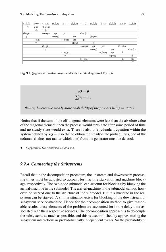
9.2 Modeling The Two-Node Subsystem 291
(1,0,0) (2,0,0) (1,1,1) (1,2,1) (2,1,1) (2,2,1) (1,1,2) (1,2,2) (2,1,2) (2,2,2) (b,1,2) (b,2,2) − α p α (1−p) α
−β β (1−q)μ −(α+μ) qμ pα (1−p)α
γ −(α+γ) pα (1−p)α (1−q)μ −(β+μ) qμ β γ −(β+γ) β (1−q)μ −(α+μ) qμ pα (1−p) α γ −(α+γ) pα (1−p) α (1−q)μ −(β+μ) qμ β γ −(β+γ) β (1−q)μ −μ qμ γ −γ
Fig. 9.7 Q-generator matrix associated with the rate diagram of Fig. 9.6
vQ = 0
∑i
vi = 1 ,
then vi denotes the steady-state probability of the process being in state i.
Notice that if the sum of the off-diagonal elements were less than the absolute valueof the diagonal element, then the process would terminate after some period of timeand no steady-state would exist. There is also one redundant equation within thesystem defined by vQ = 0 so that to obtain the steady-state probabilities, one of thecolumns (it does not matter which one) from the generator must be deleted.
• Suggestion: Do Problems 9.4 and 9.5.
9.2.4 Connecting the Subsystems
Recall that in the decomposition procedure, the upstream and downstream process-ing times must be adjusted to account for machine starvation and machine block-age, respectively. The two-node submodel can account for blocking by blocking thearrival-machine in the submodel. The arrival-machine in the submodel cannot, how-ever, be starved due to the structure of the submodel. But this machine in the realsystem can be starved. A similar situation exists for blocking of the downstream orsubsystem service-machine. Hence for the decomposition method to give reason-able results, these elements of the problem are accounted for in the delay time as-sociated with their respective services. The decomposition approach is to de-couplethe subsystems as much as possible, and this is accomplished by approximating thesubsystem interactions as probabilistically independent events. So the probability of
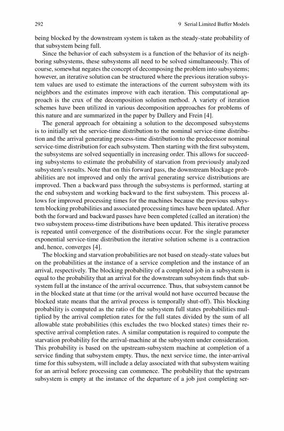
292 9 Serial Limited Buffer Models
being blocked by the downstream system is taken as the steady-state probability ofthat subsystem being full.
Since the behavior of each subsystem is a function of the behavior of its neigh-boring subsystems, these subsystems all need to be solved simultaneously. This ofcourse, somewhat negates the concept of decomposing the problem into subsystems;however, an iterative solution can be structured where the previous iteration subsys-tem values are used to estimate the interactions of the current subsystem with itsneighbors and the estimates improve with each iteration. This computational ap-proach is the crux of the decomposition solution method. A variety of iterationschemes have been utilized in various decomposition approaches for problems ofthis nature and are summarized in the paper by Dallery and Frein [4].
The general approach for obtaining a solution to the decomposed subsystemsis to initially set the service-time distribution to the nominal service-time distribu-tion and the arrival generating process-time distribution to the predecessor nominalservice-time distribution for each subsystem. Then starting with the first subsystem,the subsystems are solved sequentially in increasing order. This allows for succeed-ing subsystems to estimate the probability of starvation from previously analyzedsubsystem’s results. Note that on this forward pass, the downstream blockage prob-abilities are not improved and only the arrival generating service distributions areimproved. Then a backward pass through the subsystems is performed, starting atthe end subsystem and working backward to the first subsystem. This process al-lows for improved processing times for the machines because the previous subsys-tem blocking probabilities and associated processing times have been updated. Afterboth the forward and backward passes have been completed (called an iteration) thetwo subsystem process-time distributions have been updated. This iterative processis repeated until convergence of the distributions occur. For the single parameterexponential service-time distribution the iterative solution scheme is a contractionand, hence, converges [4].
The blocking and starvation probabilities are not based on steady-state values buton the probabilities at the instance of a service completion and the instance of anarrival, respectively. The blocking probability of a completed job in a subsystem isequal to the probability that an arrival for the downstream subsystem finds that sub-system full at the instance of the arrival occurrence. Thus, that subsystem cannot bein the blocked state at that time (or the arrival would not have occurred because theblocked state means that the arrival process is temporally shut-off). This blockingprobability is computed as the ratio of the subsystem full states probabilities mul-tiplied by the arrival completion rates for the full states divided by the sum of allallowable state probabilities (this excludes the two blocked states) times their re-spective arrival completion rates. A similar computation is required to compute thestarvation probability for the arrival-machine at the subsystem under consideration.This probability is based on the upstream-subsystem machine at completion of aservice finding that subsystem empty. Thus, the next service time, the inter-arrivaltime for this subsystem, will include a delay associated with that subsystem waitingfor an arrival before processing can commence. The probability that the upstreamsubsystem is empty at the instance of the departure of a job just completing ser-

9.3 Example of a Kanban Serial System 293
M0M 2M 3MB1 B2 B3
3 4/3
Fig. 9.8 Diagram representation of the example problem of Sect. 9.3 where circles represent ma-chines with mean times listed and boxes representW IP buffer areas with capacities listed
vice is computed based on the service completion rates for the various upstreamsubsystem states excluding the empty states (no service event can occur while thatsubsystem is empty and, therefore, not serving a job). The starvation probability forthe subsystem in question is then the ratio of the sum of the probabilities that thissubsystem has only one job in it times the job completion rates for those states andthe sum of all nonzero states times their respective service-completion rates.
A detailed example is used to illustrate this iteration solution scheme. This sim-ple three workstation serial system with exponential service time distributions con-verges to an acceptable accuracy level in 5 iterations. The errors as compared with asingle long simulation run are in the neighborhood of 1% for the three performancemeasures of cycle time, throughput and work-in-process.
9.3 Example of a Kanban Serial System
A kanban system has been implemented within a facility that has a simple serialstructure for its three workstations. The kanban limits are 4, 3, and 4, respectively,at the three workstations. All three workstations are single machine systems withexponential processing times have means of 80 min, 75 min, and 72 min, respec-tively. When there is room to begin a new job in the first workstation (i.e., when anew job is pulled into the factory), it takes an average of 60 minutes to gather theraw material and do the data entry necessary to begin the job within the factory.Notice that in Fig. 9.8 illustrating this factory, the capacity of the buffers is one lessthan the kanban limits due to a job possibly being in process.
Since the factory is using a kanban control system, each machine is blockedfrom starting service on a new job until the job just completed obtains space in thenext workstation. The first or job arrival generating machine is always busy exceptwhen it has a completed job that is blocked from entering the first workstation. Thissituation blocks the machine from starting on a new job. Completed jobs at the lastworkstation leave the system with no blockage or delays.
Throughout the discussion of the algorithm, it will be important to keep in mindthe distinction between the arrival-machine and the service-machine. The first sub-system contains the machine pair (0, 1) with Machine 0 being the arrival-machineand Machine 1 being the service-machine. The second subsystem contains the ma-chine pair (1,2) with Machine 1 being the arrival-machine and Machine 2 being the
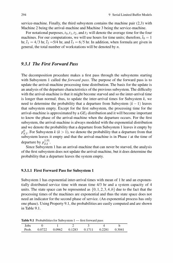
294 9 Serial Limited Buffer Models
service-machine. Finally, the third subsystem contains the machine pair (2,3) withMachine 2 being the arrival-machine and Machine 3 being the service-machine.
For notational purposes, t0, t1, t2, and t3 will denote the average time for the fourmachines. For our computations, we will use hours for time units; therefore, t0 = 1hr, t1 = 4/3 hr, t2 =5/4 hr, and t3 = 6/5 hr. In addition, when formula are given ingeneral, the total number of workstations will be denoted by n.
9.3.1 The First Forward Pass
The decomposition procedure makes a first pass through the subsystems startingwith Subsystem 1 called the forward pass. The purpose of the forward pass is toupdate the arrival-machine processing time distribution. The basis for the update isan analysis of the departure characteristics of the previous subsystem. The difficultywith the arrival-machine is that it might become starved and so the inter-arrival timeis longer than normal; thus, to update the inter-arrival times for Subsystem k, weneed to determine the probability that a departure from Subsystem (k− 1) leavesthat subsystem empty. Except for the first subsystem, the processing time for thearrival-machine is approximated by a GE2 distribution and it will become importantto know the phase of the arrival-machine when the departure occurs. For the firstsubsystem, the arrival-machine is always modeled with the exponential distributionand we denote the probability that a departure from Subsystem 1 leaves it empty byp0
d,1. For Subsystem k (k > 1), we denote the probability that a departure from thatsubsystem leaves it empty and that the arrival-machine is in Phase i at the time of
departure by p(i,0)d,k .
Since Subsystem 1 has an arrival-machine that can never be starved, the analysisof the first subsystem does not update the arrival-machine, but it does determine theprobability that a departure leaves the system empty.
9.3.1.1 First Forward Pass for Subsystem 1
Subsystem 1 has exponential inter-arrival times with mean of 1 hr and an exponen-tially distributed service time with mean time 4/3 hr and a system capacity of 4units. The state space can be represented as {0,1,2,3,4,b} due to the fact that theprocessing times of the machines are exponential and thus the state space does notneed an indicator for the second phase of service. (An exponential process has onlyone phase). Using Property 9.1, the probabilities are easily computed and are shownin Table 9.1.
Table 9.1 Probabilities for Subsystem 1 — first forward pass
Jobs 0 1 2 3 4 bProb. 0.0722 0.0962 0.1283 0.1711 0.2281 0.3041

9.3 Example of a Kanban Serial System 295
The probability that a departure leaves the subsystem empty is the probabilitythat this job was the only job in the subsystem at the departure time. Note that nodeparture can occur if the subsystem is empty. Thus, this probability is computed asthe conditional probability (Definition 1.3) that there is one job in the system giventhat system in not empty; that is,
p0d,1 =
0.09621−0.0722
= 0.1037 .
The throughput rate for this subsystem is based on the steady-state probabilitiesand is computed from the mean arrival rate times the probability that the system isnot blocked. Thus, the throughput rate for subsystem one is
th(1) = 1× (1−0.3041)= 0.6959/hr .
Summary: The first forward pass of Subsystem 1 will always use probabilitiesderived from Property 9.1. Assume these probabilities are denoted by vi for i =0, · · · ,wmax +1, where wmax +1 represents the blocked state. (For ease of notation,we shall let vwmax be written as vmax and let vwmax+1 be written as vb.) Then theprobability that a departure will leave the system empty is
p0d,1 =
v1
1− v0, (9.4)
and the mean throughput rate is given by
th(1) =1− vb
t0, (9.5)
where t0 is the mean time needed to release jobs into the factory (or the time toprepare jobs for processing) once there is room available.
9.3.1.2 First Forward Pass for Subsystem 2
The second subsystem has Machine 1 as the arrival-machine and Machine 2 as theservice-machine. The buffer for this subsystem has a limit of 2 therefore its capac-ity is 3 units. For the first pass, the service distribution is exponential with meantime 5/4 hr. The inter-arrival time distribution used for the arrival-machine is themachine’s nominal service time (exponentially distributed with mean time 4/3 hror, equivalently, a mean rate of 0.75/hr) interspersed with periodic delays due tomachine starvation. That is, periodically this arrival-machine (that is really the ma-chine for Subsystem 1) does not have a job to process and must wait for its ownarrival which is exponentially distributed with a mean time of 1 hr. Thus, when anarrival occurs to Subsystem 2, this job departs from Subsystem 1 and if it leavesthat subsystem empty, the time until the next departure includes both the idle timeof Machine 1 plus the service time of Machine 1. Therefore, the probability that
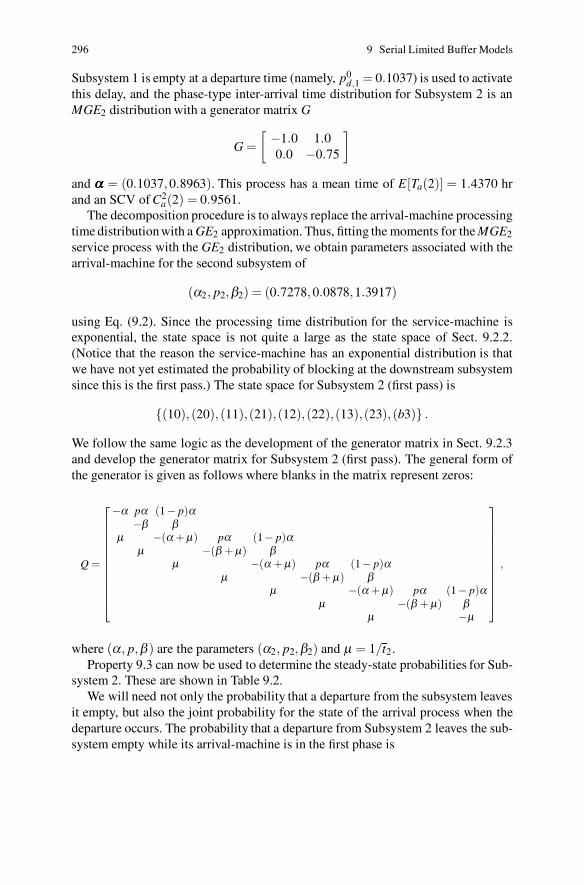
296 9 Serial Limited Buffer Models
Subsystem 1 is empty at a departure time (namely, p0d,1 = 0.1037) is used to activate
this delay, and the phase-type inter-arrival time distribution for Subsystem 2 is anMGE2 distribution with a generator matrix G
G =[
−1.0 1.00.0 −0.75
]
and ααα = (0.1037,0.8963). This process has a mean time of E[Ta(2)] = 1.4370 hrand an SCV of C2
a(2) = 0.9561.The decomposition procedure is to always replace the arrival-machine processing
time distribution with a GE2 approximation. Thus, fitting the moments for the MGE2
service process with the GE2 distribution, we obtain parameters associated with thearrival-machine for the second subsystem of
(α2, p2,β2) = (0.7278,0.0878,1.3917)
using Eq. (9.2). Since the processing time distribution for the service-machine isexponential, the state space is not quite a large as the state space of Sect. 9.2.2.(Notice that the reason the service-machine has an exponential distribution is thatwe have not yet estimated the probability of blocking at the downstream subsystemsince this is the first pass.) The state space for Subsystem 2 (first pass) is
{(10), (20), (11),(21),(12),(22),(13),(23), (b3)} .
We follow the same logic as the development of the generator matrix in Sect. 9.2.3and develop the generator matrix for Subsystem 2 (first pass). The general form ofthe generator is given as follows where blanks in the matrix represent zeros:
Q =
⎡
⎢
⎢
⎢
⎢
⎢
⎢
⎢
⎢
⎢
⎢
⎢
⎣
−α pα (1− p)α−β β
μ −(α + μ) pα (1− p)αμ −(β + μ) β
μ −(α + μ) pα (1− p)αμ −(β + μ) β
μ −(α + μ) pα (1− p)αμ −(β + μ) β
μ −μ
⎤
⎥
⎥
⎥
⎥
⎥
⎥
⎥
⎥
⎥
⎥
⎥
⎦
,
where (α, p,β ) are the parameters (α2, p2,β2) and μ = 1/t2.Property 9.3 can now be used to determine the steady-state probabilities for Sub-
system 2. These are shown in Table 9.2.We will need not only the probability that a departure from the subsystem leaves
it empty, but also the joint probability for the state of the arrival process when thedeparture occurs. The probability that a departure from Subsystem 2 leaves the sub-system empty while its arrival-machine is in the first phase is
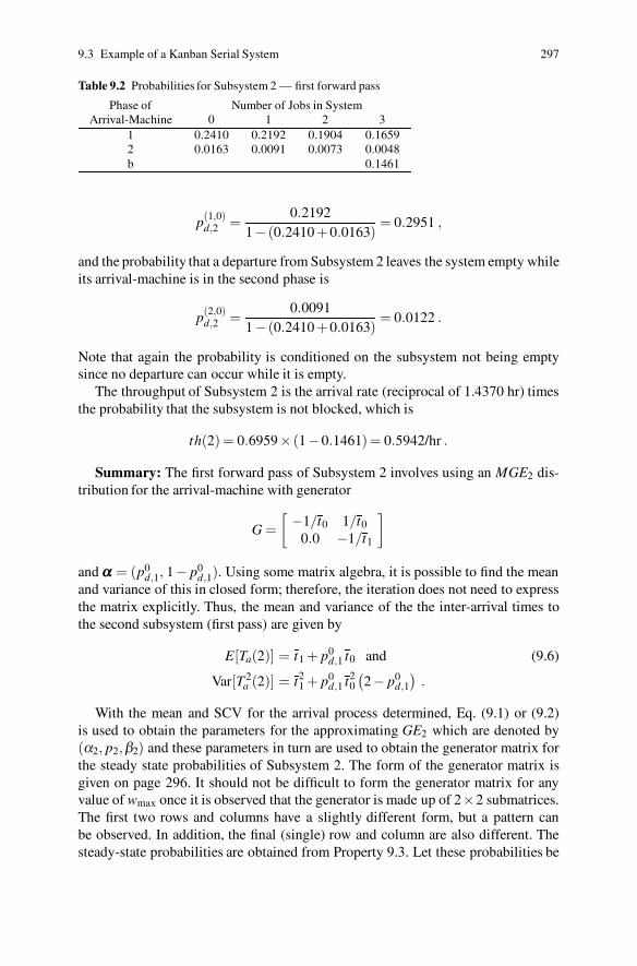
9.3 Example of a Kanban Serial System 297
Table 9.2 Probabilities for Subsystem 2 — first forward pass
Phase of Number of Jobs in SystemArrival-Machine 0 1 2 3
1 0.2410 0.2192 0.1904 0.16592 0.0163 0.0091 0.0073 0.0048b 0.1461
p(1,0)d,2 =
0.21921− (0.2410 +0.0163)
= 0.2951 ,
and the probability that a departure from Subsystem 2 leaves the system empty whileits arrival-machine is in the second phase is
p(2,0)d,2 =
0.00911− (0.2410 +0.0163)
= 0.0122 .
Note that again the probability is conditioned on the subsystem not being emptysince no departure can occur while it is empty.
The throughput of Subsystem 2 is the arrival rate (reciprocal of 1.4370 hr) timesthe probability that the subsystem is not blocked, which is
th(2) = 0.6959× (1−0.1461)= 0.5942/hr .
Summary: The first forward pass of Subsystem 2 involves using an MGE2 dis-tribution for the arrival-machine with generator
G =[
−1/t0 1/t0
0.0 −1/t1
]
and ααα = (p0d,1, 1− p0
d,1). Using some matrix algebra, it is possible to find the meanand variance of this in closed form; therefore, the iteration does not need to expressthe matrix explicitly. Thus, the mean and variance of the the inter-arrival times tothe second subsystem (first pass) are given by
E[Ta(2)] = t1 + p0d,1 t0 and (9.6)
Var[T 2a (2)] = t2
1 + p0d,1 t2
0
(
2− p0d,1
)
.
With the mean and SCV for the arrival process determined, Eq. (9.1) or (9.2)is used to obtain the parameters for the approximating GE2 which are denoted by(α2, p2,β2) and these parameters in turn are used to obtain the generator matrix forthe steady state probabilities of Subsystem 2. The form of the generator matrix isgiven on page 296. It should not be difficult to form the generator matrix for anyvalue of wmax once it is observed that the generator is made up of 2×2 submatrices.The first two rows and columns have a slightly different form, but a pattern canbe observed. In addition, the final (single) row and column are also different. Thesteady-state probabilities are obtained from Property 9.3. Let these probabilities be
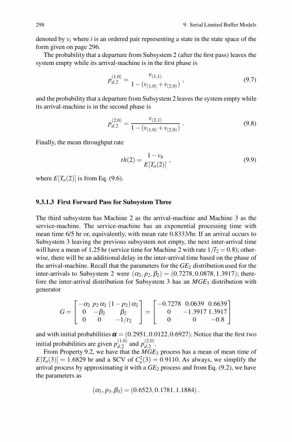
298 9 Serial Limited Buffer Models
denoted by vi where i is an ordered pair representing a state in the state space of theform given on page 296.
The probability that a departure from Subsystem 2 (after the first pass) leaves thesystem empty while its arrival-machine is in the first phase is
p(1,0)d,2 =
v(1,1)
1− (v(1,0) + v(2,0)), (9.7)
and the probability that a departure from Subsystem 2 leaves the system empty whileits arrival-machine is in the second phase is
p(2,0)d,2 =
v(2,1)
1− (v(1,0) + v(2,0)). (9.8)
Finally, the mean throughput rate
th(2) =1− vb
E[Ta(2)], (9.9)
where E[Ta(2)] is from Eq. (9.6).
9.3.1.3 First Forward Pass for Subsystem Three
The third subsystem has Machine 2 as the arrival-machine and Machine 3 as theservice-machine. The service-machine has an exponential processing time withmean time 6/5 hr or, equivalently, with mean rate 0.8333/hr. If an arrival occurs toSubsystem 3 leaving the previous subsystem not empty, the next inter-arrival timewill have a mean of 1.25 hr (service time for Machine 2 with rate 1/t2 = 0.8); other-wise, there will be an additional delay in the inter-arrival time based on the phase ofthe arrival-machine. Recall that the parameters for the GE2 distribution used for theinter-arrivals to Subsystem 2 were (α2, p2,β2) = (0.7278,0.0878,1.3917); there-fore the inter-arrival distribution for Subsystem 3 has an MGE3 distribution withgenerator
G =
⎡
⎣
−α2 p2 α2 (1− p2)α2
0 −β2 β2
0 0 −1/t2
⎤
⎦=
⎡
⎣
−0.7278 0.0639 0.66390 −1.3917 1.39170 0 −0.8
⎤
⎦
and with initial probabilities ααα = (0.2951,0.0122,0.6927). Notice that the first two
initial probabilities are given p(1,0)d,2 and p(2,0)
d,2 .From Property 9.2, we have that the MGE3 process has a mean of mean time of
E[Ta(3)] = 1.6829 hr and a SCV of C2a(3) = 0.9110. As always, we simplify the
arrival process by approximating it with a GE2 process and from Eq. (9.2), we havethe parameters as
(α3, p3,β3) = (0.6523,0.1781,1.1884) .
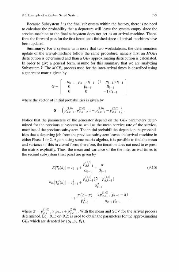
9.3 Example of a Kanban Serial System 299
Because Subsystem 3 is the final subsystem within the factory, there is no needto calculate the probability that a departure will leave the system empty since theservice-machine to the final subsystem does not act as an arrival-machine. There-fore, the forward pass for the first iteration is finished since all arrival-machines havebeen updated.
Summary: For a systems with more that two workstations, the determinationupdate of the arrival-machine follow the same procedure, namely first an MGE3
distribution is determined and than a GE2 approximating distribution is calculated.In order to give a general form, assume for this summary that we are analyzingSubsystem k. The MGE3 process used for the inter-arrival times is described usinga generator matrix given by
G =
⎡
⎣
−αk−1 pk−1 αk−1 (1− pk−1)αk−1
0 −βk−1 βk−10 0 −1/tk−1
⎤
⎦
where the vector of initial probabilities is given by
ααα =(
p(1,0)d,k−1, p(2,0)
d,k−1, 1− p(1,0)d,k−1− p(2,0)
d,k−1
)
.
Notice that the parameters of the generator depend on the GE2 parameters deter-mined for the previous subsystem as well as the mean service rate of the service-machine of the previous subsystem. The initial probabilities depend on the probabil-ities that a departing job from the previous subsystem leaves the arrival-machine ineither Phase 1 or 2. Again, using some matrix algebra, it is possible to find the meanand variance of this in closed form; therefore, the iteration does not need to expressthe matrix explicitly. Thus, the mean and variance of the the inter-arrival times tothe second subsystem (first pass) are given by
E[Ta(k)] = tk−1 +p(1,0)
d,k−1
αk−1+
πβk−1
(9.10)
Var[T 2a (k)] = t2
k−1 +p(1,0)
d,k−1(2− p(1,0)d,k−1)
α2k−1
+π (2−π)
β 2k−1
+2p(1,0)
d,k−1(pk−1−π)
αk−1 βk−1,
where π = p(1,0)d,k−1× pk−1 + p(2,0)
d,k−1. With the mean and SCV for the arrival processdetermined, Eq. (9.1) or (9.2) is used to obtain the parameters for the approximatingGE2 which are denoted by (αk, pk,βk).
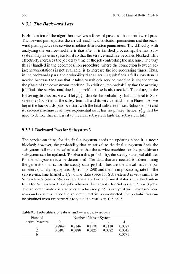
300 9 Serial Limited Buffer Models
9.3.2 The Backward Pass
Each iteration of the algorithm involves a forward pass and then a backward pass.The forward pass updates the arrival-machine distribution parameters and the back-ward pass updates the service-machine distribution parameters. The difficulty withanalyzing the service-machine is that after it is finished processing, the next sub-system may have no space for it so that the service-machine becomes blocked. Thiseffectively increases the job delay time of the job controlling the machine. The waythis is handled in the decomposition procedure, where the connection between ad-jacent workstations is not available, is to increase the job processing times. Thus,in the backwards pass, the probability that an arriving job finds a full subsystem isneeded because the time that it takes to unblock service-machine is dependent onthe phase of the downstream machine. In addition, the probability that the arrivingjob finds the service-machine in a specific phase is also needed. Therefore, in the
following discussion, we will let p(i,F)a,k denote the probability that an arrival to Sub-
system k (k < n) finds the subsystem full and its service-machine in Phase i. As webegin the backwards pass, we start with the final subsystem (i.e., Subsystem n) andits service-machine is always exponential so it has no phases; hence, pF
a,n will beused to denote that an arrival to the final subsystem finds the subsystem full.
9.3.2.1 Backward Pass for Subsystem 3
The service-machine for the final subsystem needs no updating since it is neverblocked; however, the probability that an arrival to the final subsystem finds thesubsystem full must be calculated so that the service-machine for the penultimatesubsystem can be updated. To obtain this probability, the steady-state probabilitiesfor the subsystem must be determined. The data that are needed for determiningthe generator matrix for the steady-state probabilities are the arrival-machine pa-rameters (namely, α3, p3, and β3 from p. 298) and the mean processing rate for theservice-machine (namely, 1/t3). The state space for Subsystem 3 is very similar toSubsystem 2 (see p. 296) except there are two additional states since the kanbanlimit for Subsystem 3 is 4 jobs whereas the capacity for Subsystem 2 was 3 jobs.The generator matrix is also very similar (see p. 296) except it will have two morerows and columns. Once the generator matrix is constructed, the probabilities canbe obtained from Property 9.3 to yield the results in Table 9.3.
Table 9.3 Probabilities for Subsystem 3 — first backward pass
Phase of Number of Jobs in SystemArrival-Machine 0 1 2 3 4
1 0.2869 0.2246 0.1578 0.1110 0.07872 0.0407 0.0180 0.0125 0.0082 0.0045b 0.0571

9.3 Example of a Kanban Serial System 301
The probability that an arrival finds the system full (i.e., the probability that anarrival gets blocked) is a conditional probability based on the state of the arrival-machine when the arrival occurs. (Notice that because the service-machine processis not exponential, the time-averaged probability of finding the system full is not thesame as the probability of finding the system full at a departure time.) The probabil-ity that an arrival will occur to Subsystem 3 while its arrival-machine is in Phase 1is 1− p3 = 0.8219 (recall that p3 is a parameter of the arrival-machine GE2 distribu-tion as determined by the forward pass) and it will occur while the arrival-machineis in Phase 2 with probability p3 = 0.1781. The conditional probability that the ar-riving job will find a full system given that the arrival-machine is in Phase 1 at thearrival time is
Pr{full|Arrival Phase 1} =0.0787
0.2869 +0.2246+0.1578+0.1110+0.0787= 0.0916 ,
and the conditional probability that the arriving job will find a full system given thatthe arrival-machine is in Phase 2 is
Pr{full|Arrival Phase 2) =0.0045
0.0407 +0.0180 +0.0125 +0.0082+0.0045= 0.0534 ;
therefore, the probability of blocking occuring upon an arrival from the second sub-system is
pFa,3 = 0.8219×0.0916 +0.1781×0.0534 = 0.0849 .
The throughput of Subsystem 3 is the arrival rate (the reciprocal of 1.6829 hr)times the probability that Subsystem 3 is not blocked, which is
th(3) = 0.5942× (1−0.0571)= 0.5603/hr .
Summary: The backward pass starts with the final subsystem and begins withdetermining its steady-state probabilities. The state space will always be of the formgiven on p. 296 and the generator will be similar to that on p. 296. Once the generatormatrix is constructed, Property 9.3 is used to yield the probabilities denoted as vi fori an ordered pair representing a state. The blocking probability is given by
pFa,n = (1− pn)
v(1,max)
∑maxi=0 v(1,i)
+ pnv(2,max)
∑maxi=0 v(2,i)
, (9.11)
where pn is the parameter from the approximating GE2 distribution for the arrival-machine of the final subsystem. Finally, the mean throughput rate is
th(n) =1− vb
E[Ta(n)], (9.12)
where E[Ta(n)] is from Eq. (9.10).
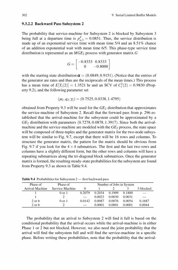
302 9 Serial Limited Buffer Models
9.3.2.2 Backward Pass Subsystem 2
The probability that service-machine for Subsystem 2 is blocked by Subsystem 3being full at a departure time is pF
a,3 = 0.0851. Thus, the service distribution ismade up of an exponential service time with mean time 5/4 and an 8.51% chanceof an addition exponential wait with mean time 6/5. This phase-type service timedistribution is represented as an MGE2 process with generator matrix G
G =[
−0.8333 0.83330 −0.8000
]
with the starting state distribution ααα = (0.0849,0.9151). (Notice that the entries ofthe generator are rates and thus are the reciprocals of the mean times.) This processhas a mean time of E[Ts(2)] = 1.3521 hr and an SCV of C2
s (2) = 0.9830 (Prop-erty 9.2), and the following parameter set
(μ2,q2, γ2) = (0.7525,0.0338,1.4795)
obtained from Property 9.3 will be used for the GE2 distribution that approximatesthe service-machine of Subsystem 2. Recall that the forward pass from p. 296 es-tablished that the arrival-machine for the subsystem could be approximated by aGE2 distribution with parameters (0.7278,0.0878,1.3917). Since both the arrival-machine and the service-machine are modeled with the GE2 process, the state spacewill be composed of three-tuples and the generator matrix for the two-node subsys-tem will be similar to Fig. 9.7, except that there will be 16 rows and columns. Tostructure the generator matrix, the pattern for the matrix should be obvious fromFig. 9.7 if you look for the 4× 4 submatrices. The first and the last two rows andcolumns have a slightly different form, but the other rows and columns will have arepeating submatrices along the tri-diagonal block submatrices. Once the generatormatrix is formed, the resulting steady-state probabilities for the subsystem are foundfrom Property 9.3 as shown in Table 9.4.
Table 9.4 Probabilities for Subsystem 2 — first backward pass
Phase of Phase of Number of Jobs in SystemArrival-Machine Service-Machine 0 1 2 3 3-blocked
1 0 or 1 0.2079 0.2034 0.1909 0.1800 —1 2 — 0.0023 0.0030 0.0031 —
2 or b 0 or 1 0.0142 0.0087 0.0076 0.0054 0.16872 or b 2 — 0.0001 0.0001 0.0001 0.0044
The probability that an arrival to Subsystem 2 will find it full is based on theconditional probability that the arrival occurs while the arrival-machine is in eitherPhase 1 or 2 but not blocked. However, we also need the joint probability that thearrival will find the subsystem full and will find the service-machine in a specificphase. Before writing these probabilities, note that the probability that the arrival-
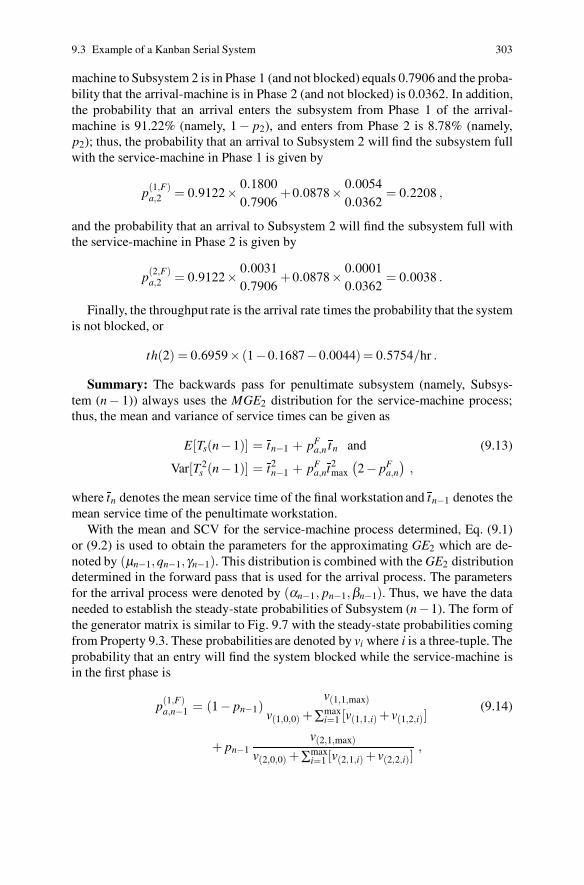
9.3 Example of a Kanban Serial System 303
machine to Subsystem 2 is in Phase 1 (and not blocked) equals 0.7906 and the proba-bility that the arrival-machine is in Phase 2 (and not blocked) is 0.0362. In addition,the probability that an arrival enters the subsystem from Phase 1 of the arrival-machine is 91.22% (namely, 1− p2), and enters from Phase 2 is 8.78% (namely,p2); thus, the probability that an arrival to Subsystem 2 will find the subsystem fullwith the service-machine in Phase 1 is given by
p(1,F)a,2 = 0.9122× 0.1800
0.7906+0.0878× 0.0054
0.0362= 0.2208 ,
and the probability that an arrival to Subsystem 2 will find the subsystem full withthe service-machine in Phase 2 is given by
p(2,F)a,2 = 0.9122× 0.0031
0.7906+0.0878× 0.0001
0.0362= 0.0038 .
Finally, the throughput rate is the arrival rate times the probability that the systemis not blocked, or
th(2) = 0.6959× (1−0.1687−0.0044)= 0.5754/hr .
Summary: The backwards pass for penultimate subsystem (namely, Subsys-tem (n− 1)) always uses the MGE2 distribution for the service-machine process;thus, the mean and variance of service times can be given as
E[Ts(n−1)] = tn−1 + pFa,n tn and (9.13)
Var[T 2s (n−1)] = t2
n−1 + pFa,nt2
max
(
2− pFa,n
)
,
where tn denotes the mean service time of the final workstation and tn−1 denotes themean service time of the penultimate workstation.
With the mean and SCV for the service-machine process determined, Eq. (9.1)or (9.2) is used to obtain the parameters for the approximating GE2 which are de-noted by (μn−1,qn−1, γn−1). This distribution is combined with the GE2 distributiondetermined in the forward pass that is used for the arrival process. The parametersfor the arrival process were denoted by (αn−1, pn−1,βn−1). Thus, we have the dataneeded to establish the steady-state probabilities of Subsystem (n−1). The form ofthe generator matrix is similar to Fig. 9.7 with the steady-state probabilities comingfrom Property 9.3. These probabilities are denoted by vi where i is a three-tuple. Theprobability that an entry will find the system blocked while the service-machine isin the first phase is
p(1,F)a,n−1 = (1− pn−1)
v(1,1,max)
v(1,0,0) +∑maxi=1 [v(1,1,i) + v(1,2,i)]
(9.14)
+ pn−1v(2,1,max)
v(2,0,0) +∑maxi=1 [v(2,1,i) + v(2,2,i)]
,
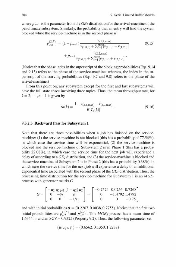
304 9 Serial Limited Buffer Models
where pn−1 is the parameter from the GE2 distribution for the arrival-machine of thepenultimate subsystem. Similarly, the probability that an entry will find the systemblocked while the service-machine is in the second phase is
p(2,F)a,n−1 = (1− pn−1)
v(1,2,max)
v(1,0,0) +∑maxi=1 [v(1,1,i) + v(1,2,i)]
(9.15)
+ pn−1v(2,2,max)
v(2,0,0) +∑maxi=1 [v(2,1,i) + v(2,2,i)]
.
(Notice that the phase index in the superscript of the blocking probabilities (Eqs. 9.14and 9.15) refers to the phase of the service-machine; whereas, the index in the su-perscript of the starving probabilities (Eqs. 9.7 and 9.8) refers to the phase of thearrival-machine.)
From this point on, any subsystem except for the first and last subsystems willhave the full state space involving three tuples. Thus, the mean throughput rate, fork = 2, · · · ,n−1 is given by
th(k) =1− v(b,1,max)− v(b,2,max)
E[Ta(k)]. (9.16)
9.3.2.3 Backward Pass for Subsystem 1
Note that there are three possibilities when a job has finished on the service-machine: (1) the service-machine is not blocked (this has a probability of 77.54%),in which case the service time will be exponential, (2) the service-machine isblocked and the service-machine of Subsystem 2 is in Phase 1 (this has a proba-bility 22.08%), in which case the service time for the next job will experience adelay of according to a GE2 distribution, and (3) the service-machine is blocked andthe service-machine of Subsystem 2 is in Phase 2 (this has a probability 0.38%), inwhich case the service time for the next job will experience a delay of an additionalexponential time associated with the second phase of the GE2 distribution. Thus, theprocessing time distribution for the service-machine for Subsystem 1 is an MGE3
process with generator matrix G
G =
⎡
⎣
−μ2 q2 μ2 (1−q2)μ2
0 −γ2 γ2
0 0 −1/t1
⎤
⎦=
⎡
⎣
−0.7524 0.0256 0.72680 −1.4792 1.47920 0 −0.75
⎤
⎦
and with initial probabilities ααα = (0.2207,0.0038,0.7755). Notice that the first two
initial probabilities are p(1,F)a,2 and p(2,F)
a,2 . This MGE3 process has a mean time of1.6344 hr and an SCV = 0.9325 (Property 9.2). Thus, the following parameter set
(μ1,q1, γ1) = (0.6562,0.1350,1.2238)
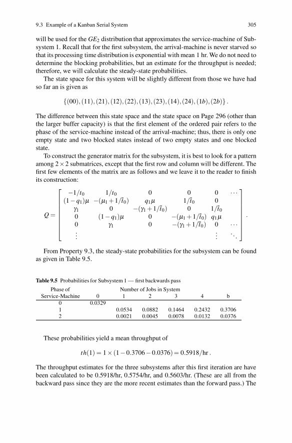
9.3 Example of a Kanban Serial System 305
will be used for the GE2 distribution that approximates the service-machine of Sub-system 1. Recall that for the first subsystem, the arrival-machine is never starved sothat its processing time distribution is exponential with mean 1 hr. We do not need todetermine the blocking probabilities, but an estimate for the throughput is needed;therefore, we will calculate the steady-state probabilities.
The state space for this system will be slightly different from those we have hadso far an is given as
{(00), (11), (21), (12),(22),(13),(23),(14),(24), (1b),(2b)} .
The difference between this state space and the state space on Page 296 (other thanthe larger buffer capacity) is that the first element of the ordered pair refers to thephase of the service-machine instead of the arrival-machine; thus, there is only oneempty state and two blocked states instead of two empty states and one blockedstate.
To construct the generator matrix for the subsystem, it is best to look for a patternamong 2×2 submatrices, except that the first row and column will be different. Thefirst few elements of the matrix are as follows and we leave it to the reader to finishits construction:
Q =
⎡
⎢
⎢
⎢
⎢
⎢
⎢
⎢
⎣
−1/t0 1/t0 0 0 0 · · ·(1−q1)μ −(μ1 +1/t0) q1μ 1/t0 0
γ1 0 −(γ1 +1/t0) 0 1/t0
0 (1−q1)μ 0 −(μ1 +1/t0) q1μ0 γ1 0 −(γ1 +1/t0) 0 · · ·...
.... . .
⎤
⎥
⎥
⎥
⎥
⎥
⎥
⎥
⎦
.
From Property 9.3, the steady-state probabilities for the subsystem can be foundas given in Table 9.5.
Table 9.5 Probabilities for Subsystem 1 — first backwards pass
Phase of Number of Jobs in SystemService-Machine 0 1 2 3 4 b
0 0.03291 0.0534 0.0882 0.1464 0.2432 0.37062 0.0021 0.0045 0.0078 0.0132 0.0376
These probabilities yield a mean throughput of
th(1) = 1× (1−0.3706−0.0376)= 0.5918/hr .
The throughput estimates for the three subsystems after this first iteration are havebeen calculated to be 0.5918/hr, 0.5754/hr, and 0.5603/hr. (These are all from thebackward pass since they are the more recent estimates than the forward pass.) The
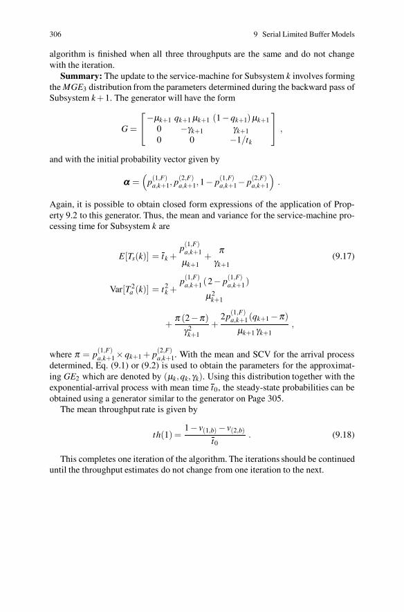
306 9 Serial Limited Buffer Models
algorithm is finished when all three throughputs are the same and do not changewith the iteration.
Summary: The update to the service-machine for Subsystem k involves formingthe MGE3 distribution from the parameters determined during the backward pass ofSubsystem k+1. The generator will have the form
G =
⎡
⎣
−μk+1 qk+1 μk+1 (1−qk+1)μk+1
0 −γk+1 γk+1
0 0 −1/tk
⎤
⎦ ,
and with the initial probability vector given by
ααα =(
p(1,F)a,k+1, p(2,F)
a,k+1,1− p(1,F)a,k+1− p(2,F)
a,k+1
)
.
Again, it is possible to obtain closed form expressions of the application of Prop-erty 9.2 to this generator. Thus, the mean and variance for the service-machine pro-cessing time for Subsystem k are
E[Ts(k)] = tk +p(1,F)
a,k+1
μk+1+
πγk+1
(9.17)
Var[T 2a (k)] = t2
k +p(1,F)
a,k+1 (2− p(1,F)a,k+1)
μ2k+1
+π (2−π)
γ2k+1
+2p(1,F)
a,k+1(qk+1 −π)
μk+1 γk+1,
where π = p(1,F)a,k+1× qk+1 + p(2,F)
a,k+1. With the mean and SCV for the arrival processdetermined, Eq. (9.1) or (9.2) is used to obtain the parameters for the approximat-ing GE2 which are denoted by (μk,qk, γk). Using this distribution together with theexponential-arrival process with mean time t0, the steady-state probabilities can beobtained using a generator similar to the generator on Page 305.
The mean throughput rate is given by
th(1) =1− v(1,b) − v(2,b)
t0. (9.18)
This completes one iteration of the algorithm. The iterations should be continueduntil the throughput estimates do not change from one iteration to the next.
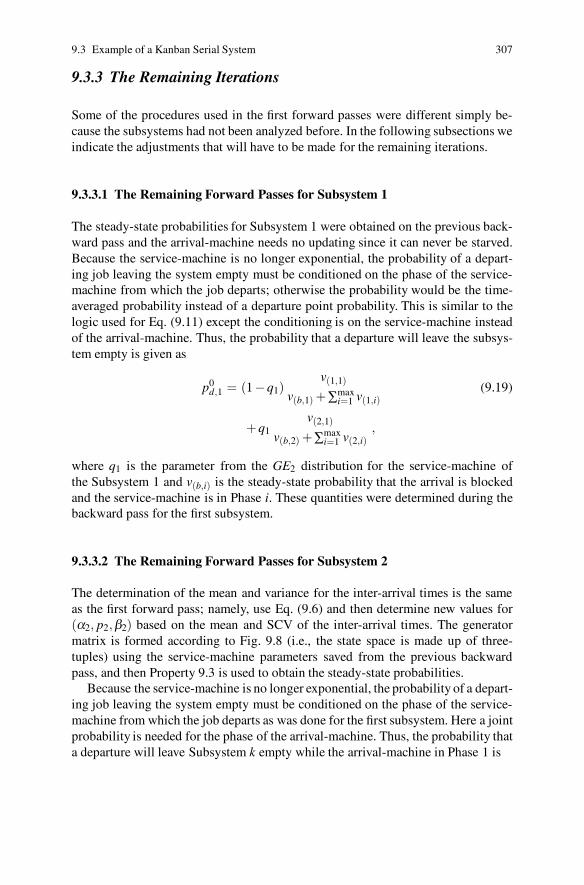
9.3 Example of a Kanban Serial System 307
9.3.3 The Remaining Iterations
Some of the procedures used in the first forward passes were different simply be-cause the subsystems had not been analyzed before. In the following subsections weindicate the adjustments that will have to be made for the remaining iterations.
9.3.3.1 The Remaining Forward Passes for Subsystem 1
The steady-state probabilities for Subsystem 1 were obtained on the previous back-ward pass and the arrival-machine needs no updating since it can never be starved.Because the service-machine is no longer exponential, the probability of a depart-ing job leaving the system empty must be conditioned on the phase of the service-machine from which the job departs; otherwise the probability would be the time-averaged probability instead of a departure point probability. This is similar to thelogic used for Eq. (9.11) except the conditioning is on the service-machine insteadof the arrival-machine. Thus, the probability that a departure will leave the subsys-tem empty is given as
p0d,1 = (1−q1)
v(1,1)
v(b,1) +∑maxi=1 v(1,i)
(9.19)
+q1v(2,1)
v(b,2) +∑maxi=1 v(2,i)
,
where q1 is the parameter from the GE2 distribution for the service-machine ofthe Subsystem 1 and v(b,i) is the steady-state probability that the arrival is blockedand the service-machine is in Phase i. These quantities were determined during thebackward pass for the first subsystem.
9.3.3.2 The Remaining Forward Passes for Subsystem 2
The determination of the mean and variance for the inter-arrival times is the sameas the first forward pass; namely, use Eq. (9.6) and then determine new values for(α2, p2,β2) based on the mean and SCV of the inter-arrival times. The generatormatrix is formed according to Fig. 9.8 (i.e., the state space is made up of three-tuples) using the service-machine parameters saved from the previous backwardpass, and then Property 9.3 is used to obtain the steady-state probabilities.
Because the service-machine is no longer exponential, the probability of a depart-ing job leaving the system empty must be conditioned on the phase of the service-machine from which the job departs as was done for the first subsystem. Here a jointprobability is needed for the phase of the arrival-machine. Thus, the probability thata departure will leave Subsystem k empty while the arrival-machine in Phase 1 is

308 9 Serial Limited Buffer Models
p(1,0)d,k = (1−qk)
v(1,1,1)
v(b,1,max) +∑maxi=1 [v(1,1,i) + v(2,1,i)]
(9.20)
+qkv(1,2,1)
v(b,2,max) +∑maxi=1 [v(1,2,i) + v(2,2,i)]
,
where qk is the parameter from the GE2 distribution for the service-machine ofSubsystem k with k = 2, · · · ,n−1. The probability that a departure will leave Sub-system k empty with the arrival-machine in Phase 2 is
p(2,0)d,k = (1−qk)
v(2,1,1)
v(b,1,max) +∑maxi=1 [v(1,1,i) + v(2,1,i)]
(9.21)
+qkv(2,2,1)
v(b,2,max) +∑maxi=1 [v(1,2,i) + v(2,2,i)]
.
9.3.3.3 The Remaining Forward and Backward Passes
The forward pass for the final subsystem and all the backward passes remain thesame as during the first iteration. Recall that one iteration includes both the forwardand backward passes. Once the throughputs converge, the decomposition algorithmis finished.
9.3.4 Convergence and Factory Performance Measures
The changing values of throughput by iteration are shown in Table 9.6 and it isseen that five iterations are sufficient for convergence. The throughput values in the
Table 9.6 Throughput results from the first five iterations
Subsystem 1 Subsystem 2 Subsystem 3Iteration 1 0.5916/hr 0.5754/hr 0.5602/hrIteration 2 0.5831/hr 0.5820/hr 0.5798/hrIteration 3 0.5824/hr 0.5823/hr 0.5821/hrIteration 4 0.5823/hr 0.5823/hr 0.5823/hrIteration 5 0.5823/hr 0.5823/hr 0.5823/hr
table are from the backwards pass. The values calculated from the forward pass areignored.
The performance measures for each workstation and the system as a whole arecomputed from the throughput rate and the steady-state probabilities for each sub-system as representative of the associated workstation. Notice that the throughputsare the same for each subsystem (0.5823/hr for our example) if convergence hastaken place, but of course, the steady-state probabilities are different. To illustrate,

9.3 Example of a Kanban Serial System 309
consider Table 9.7 that shows the steady-state probabilities for Subsystem 1 as deter-mined by the final backwards pass. The last row of the table gives the probabilities
Table 9.7 Probabilities for Subsystem 1 — fifth backwards pass
Phase of Number of Jobs in SystemService-Machine 0 1 2 3 4 b
0 0.03031 0.0501 0.0846 0.1434 0.2434 0.37452 0.0023 0.0048 0.0086 0.0148 0.0432
Sum 0.0303 0.0524 0.0894 0.1520 0.6759 —
for the number of jobs in the subsystem. Notice that the probability of 4 jobs in thesubsystem is the sum for the last two columns since the system contains 4 jobs whenit is blocked. Thus the average number of jobs in the system is
W IP(1) = 1×0.0524 +2×0.0894 +3×0.1520+4×0.6759 = 3.391 ,
and the cycle time (from Little’s Law) is
CT (1) =W IP(1)
th(1)=
3.3910.5823
= 5.823 hr .
The system WIPs is the sum of individual the WIP’s for each workstation (sub-system) and equals 7.215 jobs, and the cycle-time estimate is 7.215/0.5823 =12.391 hr. The system and individual workstation results from the analytical pro-cedure are compared with those from a simulation model. The simulation run waslong enough so that the half-width of the confidence limits for each estimate wasapproximately 1% of the estimate or smaller. The simulation and analytical com-parisons are given in Table 9.8. Both the mean throughput and cycle time errors areless that 1% and the error in the W IP estimates is less than 2%; thus, the results ofthe algorithm yield very acceptable results.
Table 9.8 Comparison of the analytical and simulation results
Analytical Simulationth W IP CT th W IP CT
System 0.5823/hr 6.798 11.674 hr 0.588/hr 6.892 11.717 hrWorkstation 1 0.5823/hr 3.391 5.823 hr 0.588/hr 3.447 5.861 hrWorkstation 2 0.5823/hr 1.784 3.063 hr 0.588/hr 1.807 3.072 hrWorkstation 3 0.5823/hr 1.623 2.787 hr 0.588/hr 1.638 2.785 hr
The results of our analysis indicate that the WIP in each workstation is signifi-cantly below the kanban limits set for system control. One reason for this is that thejob preparation time to initiate each job to the factory is on the same order as theprocess times. This is established so that the computations would result in numbers
310 9 Serial Limited Buffer Models
that could easily be checked. It is often the case that the rate at which Machine 0operates would be significantly greater than the workstation processing rates.
9.3.5 Generalizations
Serial flow networks only were considered in this presentation. General feed-forward flow networks, that is acyclic flow only with no feedback branching, werestudied by Lee and Pollock [10], and general networks that also allow backwardbranching were studied by Jun and Perros [9]. This latter problem class encountersthe phenomenon called dead-locking and these systems are difficult even to simu-late (see Deuermeyer et al. [5] and Venkatesh et al. [16]).
• Suggestion: Do Problems 9.6–9.8.
9.4 Setting Kanban Limits
A significant problem associated with the implementation of a W IP limiting con-trol strategy for factory operations is the setting of the kanban or WIP limits. Thisproblem has been studied in the literature for special cases [2, 7, 8, 14] and Chap. 7of the book by Papadopoulos, Heavey and Browne [12] discusses the results andcharacterizations of the structural properties found in the literature to that date. Arecent analysis by Spinellis, Papadopoulos and Smith [15] uses simulated annealingas the optimization tool to find the buffer settings for long production lines. Heuris-tic methods (such as simulated annealing, tabu search and genetic algorithms (see[3]) are particularly suited to the optimization of this type of problem due to thecombinatorial and stochastic nature of the problem. These methods are called meta-heuristics. According to Glover and Laguna [6]: “A meta-heuristic refers to a masterstrategy that guides and modifies other heuristics to produce solutions beyond thatnormally generated in a quest for local optimality.”
The problem is to find the individual buffer capacities (workstation WIP limits)that maximize the throughput for a given total allocation of buffer units for a se-rial system of workstations. The maximum throughput for a system without a totalbuffer-units limit is obtained by infinite queues allowed at each machine in the se-rial configuration. To make the problem realistic, the objective has been taken tofind the optimal allocation of a fixed number of buffer units. By allocation is meantthe number of buffer units to assign to each of the machines (workstations). So byfixing the total number of units available, the allocation of these units to the variousmachines so as to maximize the system throughput is a well-defined problem. Thenthe question of how many total units to allow can be answered based on a secondarycriterion such as an upper limit on the mean cycle time or reaching a minimumthroughput level.
9.4 Setting Kanban Limits 311
In this section, a scheme is developed for obtaining very good, if not optimal,buffer level configurations. Researchers such as Altiok and Stidham [2] conjecturethat the response function (throughput) is smooth and convex in nature. The exam-ple problem discussed below demonstrates that this function is not actually convexfor all cases. Thus, the solution methodology must deal with local maxima thatare not the global maximum. The general search strategy is to use a neighborhoodsearch procedure for finding local maxima in conjunction with a restart proceduredesigned to explore the solution space beyond these local maxima. The underly-ing throughput evaluation methodology is the decomposition approach (mean-valueresponse generator) discussed in this chapter. The approach developed herein canbe viewed as a particular application of tabu search, but apparently the complexmeta-heuristic structure commonly used for non-convex combinatorial problemsis not needed. For example, the approach in [15] of using simulated annealing ismuch more complex than appears necessary for the buffer allocation problem. Theirheuristic methodology, however, allows for the simultaneous optimization of bufferallocations and machine processing rates. This combined optimization is a muchmore difficult problem that requires this more powerful approach.
9.4.1 Allocating a Fixed Number of Buffer Units
For a given number of buffer space units, the problem is to find the best allocation ofthese units across the workstations so as to maximize the system throughput. Sincethis total must remain constant, it seems reasonable to use an exchange algorithmwhere a single unit is taken from one workstation and assigned to another. Then thethroughput for this new configuration is evaluated. The basic step of the algorithmis to evaluate all single units exchanges (both positive and negative) for each pairof workstations (this is called a cycle). A cycle results in n(n−1) evaluations for an workstation problem. The best configuration for all these exchanges is stored asthe current best (incumbent solution) and the process repeated. If the best exchangevalue is not better than the incumbent solution, then the process has reached a localmaximum. In this way a local search is performed with the best configuration beingused as the base point for further explorations (cycles). For concave functions thislocal search procedure converges to the global maximum.
Once a local maximum has been obtained, the pair-wise exchange of a single unitof buffer space between two workstations cannot find a better point and each addi-tional cycle will terminate again with this same solution. To allow the explorationto continue, a restart procedure is initiated once a local maximum has been identi-fied. The restart procedure implemented herein is to start the unit-exchange processfrom the local maximum with this configuration’s throughput value set to zero (anincumbent value of zero). This allows the unit-exchange process to find the secondbest point in the neighborhood as the solution obtained during the cycle since thestarting point (configuration) cannot be generated by this exchange procedure. Theneighborhood search (cycle procedure) continues from this solution. This one-unit
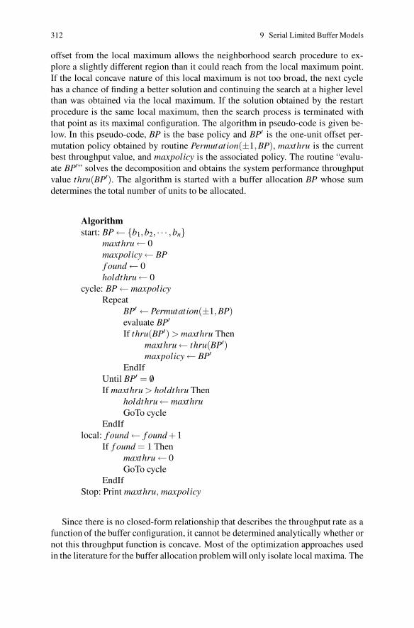
312 9 Serial Limited Buffer Models
offset from the local maximum allows the neighborhood search procedure to ex-plore a slightly different region than it could reach from the local maximum point.If the local concave nature of this local maximum is not too broad, the next cyclehas a chance of finding a better solution and continuing the search at a higher levelthan was obtained via the local maximum. If the solution obtained by the restartprocedure is the same local maximum, then the search process is terminated withthat point as its maximal configuration. The algorithm in pseudo-code is given be-low. In this pseudo-code, BP is the base policy and BP′ is the one-unit offset per-mutation policy obtained by routine Permutation(±1,BP), maxthru is the currentbest throughput value, and maxpolicy is the associated policy. The routine “evalu-ate BP′” solves the decomposition and obtains the system performance throughputvalue thru(BP′). The algorithm is started with a buffer allocation BP whose sumdetermines the total number of units to be allocated.
Algorithmstart: BP ← {b1,b2, · · · ,bn}
maxthru ← 0maxpolicy ← BPf ound ← 0holdthru← 0
cycle: BP ← maxpolicyRepeat
BP′ ← Permutation(±1,BP)evaluate BP′
If thru(BP′) > maxthru Thenmaxthru ← thru(BP′)maxpolicy ← BP′
EndIfUntil BP′ = /0If maxthru > holdthru Then
holdthru← maxthruGoTo cycle
EndIflocal: f ound ← f ound +1
If f ound = 1 Thenmaxthru ← 0GoTo cycle
EndIfStop: Print maxthru, maxpolicy
Since there is no closed-form relationship that describes the throughput rate as afunction of the buffer configuration, it cannot be determined analytically whether ornot this throughput function is concave. Most of the optimization approaches usedin the literature for the buffer allocation problem will only isolate local maxima. The
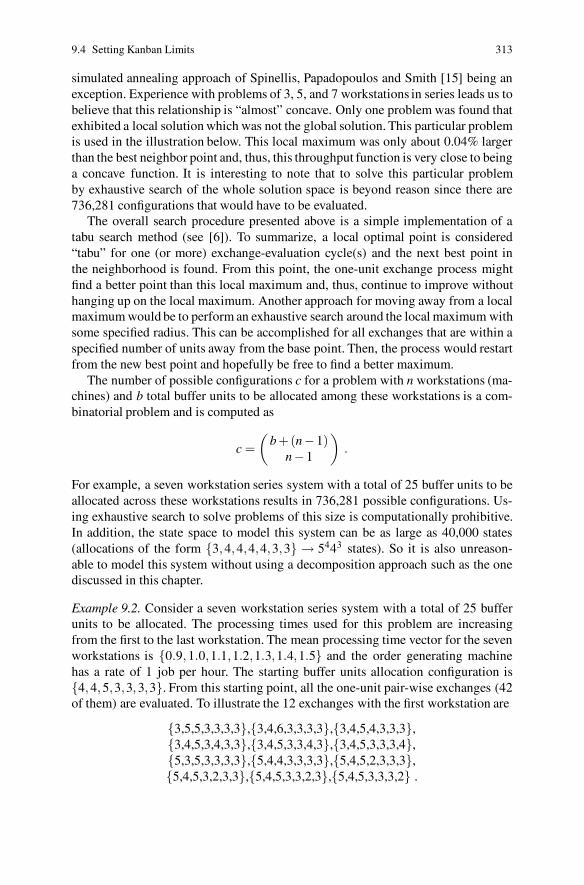
9.4 Setting Kanban Limits 313
simulated annealing approach of Spinellis, Papadopoulos and Smith [15] being anexception. Experience with problems of 3, 5, and 7 workstations in series leads us tobelieve that this relationship is “almost” concave. Only one problem was found thatexhibited a local solution which was not the global solution. This particular problemis used in the illustration below. This local maximum was only about 0.04% largerthan the best neighbor point and, thus, this throughput function is very close to beinga concave function. It is interesting to note that to solve this particular problemby exhaustive search of the whole solution space is beyond reason since there are736,281 configurations that would have to be evaluated.
The overall search procedure presented above is a simple implementation of atabu search method (see [6]). To summarize, a local optimal point is considered“tabu” for one (or more) exchange-evaluation cycle(s) and the next best point inthe neighborhood is found. From this point, the one-unit exchange process mightfind a better point than this local maximum and, thus, continue to improve withouthanging up on the local maximum. Another approach for moving away from a localmaximum would be to perform an exhaustive search around the local maximum withsome specified radius. This can be accomplished for all exchanges that are within aspecified number of units away from the base point. Then, the process would restartfrom the new best point and hopefully be free to find a better maximum.
The number of possible configurations c for a problem with n workstations (ma-chines) and b total buffer units to be allocated among these workstations is a com-binatorial problem and is computed as
c =(
b +(n−1)n−1
)
.
For example, a seven workstation series system with a total of 25 buffer units to beallocated across these workstations results in 736,281 possible configurations. Us-ing exhaustive search to solve problems of this size is computationally prohibitive.In addition, the state space to model this system can be as large as 40,000 states(allocations of the form {3,4,4,4,4,3,3} → 5443 states). So it is also unreason-able to model this system without using a decomposition approach such as the onediscussed in this chapter.
Example 9.2. Consider a seven workstation series system with a total of 25 bufferunits to be allocated. The processing times used for this problem are increasingfrom the first to the last workstation. The mean processing time vector for the sevenworkstations is {0.9,1.0,1.1,1.2,1.3,1.4,1.5} and the order generating machinehas a rate of 1 job per hour. The starting buffer units allocation configuration is{4,4,5,3,3,3,3}. From this starting point, all the one-unit pair-wise exchanges (42of them) are evaluated. To illustrate the 12 exchanges with the first workstation are
{3,5,5,3,3,3,3},{3,4,6,3,3,3,3},{3,4,5,4,3,3,3},{3,4,5,3,4,3,3},{3,4,5,3,3,4,3},{3,4,5,3,3,3,4},{5,3,5,3,3,3,3},{5,4,4,3,3,3,3},{5,4,5,2,3,3,3},{5,4,5,3,2,3,3},{5,4,5,3,3,2,3},{5,4,5,3,3,3,2} .
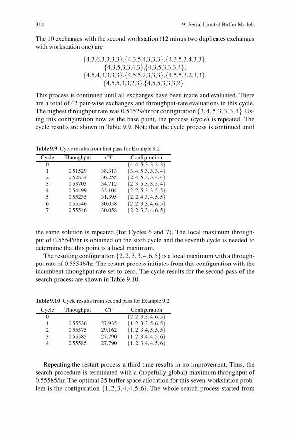
314 9 Serial Limited Buffer Models
The 10 exchanges with the second workstation (12 minus two duplicates exchangeswith workstation one) are
{4,3,6,3,3,3,3},{4,3,5,4,3,3,3},{4,3,5,3,4,3,3},{4,3,5,3,3,4,3},{4,3,5,3,3,3,4},
{4,5,4,3,3,3,3},{4,5,5,2,3,3,3},{4,5,5,3,2,3,3},{4,5,5,3,3,2,3},{4,5,5,3,3,3,2} .
This process is continued until all exchanges have been made and evaluated. Thereare a total of 42 pair-wise exchanges and throughput-rate evaluations in this cycle.The highest throughput rate was 0.51529/hr for configuration {3,4,5,3,3,3,4}. Us-ing this configuration now as the base point, the process (cycle) is repeated. Thecycle results are shown in Table 9.9. Note that the cycle process is continued until
Table 9.9 Cycle results from first pass for Example 9.2
Cycle Throughput CT Configuration0 {4,4,5,3,3,3,3}1 0.51529 38.313 {3,4,5,3,3,3,4}2 0.52834 36.255 {2,4,5,3,3,4,4}3 0.53703 34.712 {2,3,5,3,3,5,4}4 0.54499 32.104 {2,2,5,3,3,5,5}5 0.55235 31.395 {2,2,4,3,4,5,5}6 0.55546 30.058 {2,2,3,3,4,6,5}7 0.55546 30.058 {2,2,3,3,4,6,5}
the same solution is repeated (for Cycles 6 and 7). The local maximum through-put of 0.55546/hr is obtained on the sixth cycle and the seventh cycle is needed todetermine that this point is a local maximum.
The resulting configuration {2,2,3,3,4,6,5} is a local maximum with a through-put rate of 0.55546/hr. The restart process initiates from this configuration with theincumbent throughput rate set to zero. The cycle results for the second pass of thesearch process are shown in Table 9.10.
Table 9.10 Cycle results from second pass for Example 9.2
Cycle Throughput CT Configuration0 {2,2,3,3,4,6,5}1 0.55536 27.935 {1,2,3,3,5,6,5}2 0.55575 29.162 {1,2,3,4,5,5,5}3 0.55585 27.790 {1,2,3,4,4,5,6}4 0.55585 27.790 {1,2,3,4,4,5,6}
Repeating the restart process a third time results in no improvement. Thus, thesearch procedure is terminated with a (hopefully global) maximum throughput of0.55585/hr. The optimal 25 buffer space allocation for this seven-workstation prob-lem is the configuration {1,2,3,4,4,5,6}. The whole search process started from
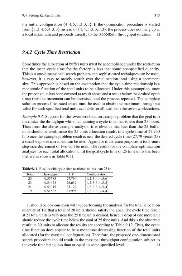
9.4 Setting Kanban Limits 315
the initial configuration {4,4,5,3,3,3,3}. If the optimization procedure is startedfrom {3,3,4,5,4,3,3} instead of {4,4,5,3,3,3,3}, the process does not hang up ata local maximum and proceeds directly to the 0.55585/hr throughput solution. ��
9.4.2 Cycle Time Restriction
Sometimes the allocation of buffer units must be accomplished under the restrictionthat the mean cycle time for the factory is less that some pre-specified quantity.This is a one-dimensional search problem and sophisticated techniques can be used,however, it is easy to merely search over the allocation total using a decrementsize. This approach is based on the assumption that the cycle-time relationship is amonotonic function of the total units to be allocated. Under this assumption, oncethe proper value has been covered (a result above and a result below the desired cycletime) then the increment can be decreased and the process repeated. The completesolution process illustrated above must be used to obtain the maximum throughputvalue for each specified total units available for allocation to the seven workstations.
Example 9.3. Suppose for the seven-workstation example problem that the goal is tomaximize the throughput while maintaining a cycle time that is less than 25 hours.Then from the above example analysis, it is obvious that less than the 25 bufferunits should be used, since the 25 units allocation results in a cycle time of 27.790hr. Since the example problem result is near the desired cycle time (27.79 verses 25)a small step-size increment can be used. Again for illustration purposes, a total-unitsstep-size decrement of two will be used. The results for the complete optimizationanalyses for each total allocation until the goal cycle time of 25 time units has beenmet are as shown in Table 9.11.
Table 9.11 Results with cycle time restricted to less than 25 hr
Total Throughput CT Configuration25 0.55585 27.790 {1,2,3,4,4,5,6}23 0.54473 26.659 {1,2,3,3,4,5,5}21 0.53015 25.122 {1,2,2,3,4,5,4}19 0.51522 23.995 {1,2,2,3,3,4,4}
It should be obvious even without performing the analysis for the total allocationquantity of 19, that a total of 20 units should satisfy the goal. The cycle time resultat 21 total units is very near the 25 time units desired, hence, a drop of one more unitshould reduce the cycle time below the goal of 25 time units. And this is the observedresult; at 20 units to allocate the results are according to Table 9.12. Thus, the cycletime function does appear to be a monotone decreasing function of the total unitsallocated (for the maximal configuration). Therefore, the proposed one-dimensionalsearch procedure should result in the maximal throughput configuration subject tothe cycle time being less than or equal to some specified level. ��
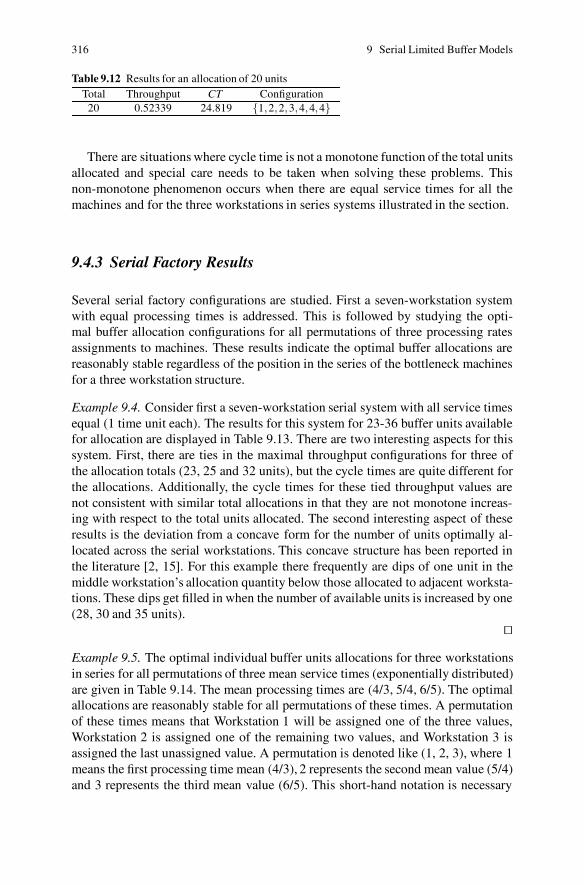
316 9 Serial Limited Buffer Models
Table 9.12 Results for an allocation of 20 unitsTotal Throughput CT Configuration
20 0.52339 24.819 {1,2,2,3,4,4,4}
There are situations where cycle time is not a monotone function of the total unitsallocated and special care needs to be taken when solving these problems. Thisnon-monotone phenomenon occurs when there are equal service times for all themachines and for the three workstations in series systems illustrated in the section.
9.4.3 Serial Factory Results
Several serial factory configurations are studied. First a seven-workstation systemwith equal processing times is addressed. This is followed by studying the opti-mal buffer allocation configurations for all permutations of three processing ratesassignments to machines. These results indicate the optimal buffer allocations arereasonably stable regardless of the position in the series of the bottleneck machinesfor a three workstation structure.
Example 9.4. Consider first a seven-workstation serial system with all service timesequal (1 time unit each). The results for this system for 23-36 buffer units availablefor allocation are displayed in Table 9.13. There are two interesting aspects for thissystem. First, there are ties in the maximal throughput configurations for three ofthe allocation totals (23, 25 and 32 units), but the cycle times are quite different forthe allocations. Additionally, the cycle times for these tied throughput values arenot consistent with similar total allocations in that they are not monotone increas-ing with respect to the total units allocated. The second interesting aspect of theseresults is the deviation from a concave form for the number of units optimally al-located across the serial workstations. This concave structure has been reported inthe literature [2, 15]. For this example there frequently are dips of one unit in themiddle workstation’s allocation quantity below those allocated to adjacent worksta-tions. These dips get filled in when the number of available units is increased by one(28, 30 and 35 units).
��
Example 9.5. The optimal individual buffer units allocations for three workstationsin series for all permutations of three mean service times (exponentially distributed)are given in Table 9.14. The mean processing times are (4/3, 5/4, 6/5). The optimalallocations are reasonably stable for all permutations of these times. A permutationof these times means that Workstation 1 will be assigned one of the three values,Workstation 2 is assigned one of the remaining two values, and Workstation 3 isassigned the last unassigned value. A permutation is denoted like (1, 2, 3), where 1means the first processing time mean (4/3), 2 represents the second mean value (5/4)and 3 represents the third mean value (6/5). This short-hand notation is necessary
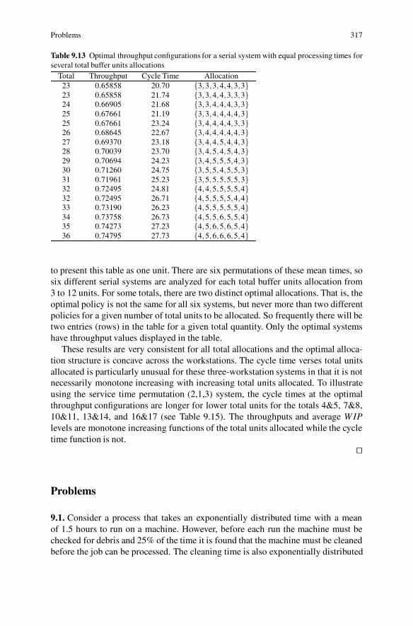
Problems 317
Table 9.13 Optimal throughput configurations for a serial system with equal processing times forseveral total buffer units allocations
Total Throughput Cycle Time Allocation23 0.65858 20.70 {3,3,3,4,4,3,3}23 0.65858 21.74 {3,3,4,4,3,3,3}24 0.66905 21.68 {3,3,4,4,4,3,3}25 0.67661 21.19 {3,3,4,4,4,4,3}25 0.67661 23.24 {3,4,4,4,4,3,3}26 0.68645 22.67 {3,4,4,4,4,4,3}27 0.69370 23.18 {3,4,4,5,4,4,3}28 0.70039 23.70 {3,4,5,4,5,4,3}29 0.70694 24.23 {3,4,5,5,5,4,3}30 0.71260 24.75 {3,5,5,4,5,5,3}31 0.71961 25.23 {3,5,5,5,5,5,3}32 0.72495 24.81 {4,4,5,5,5,5,4}32 0.72495 26.71 {4,5,5,5,5,4,4}33 0.73190 26.23 {4,5,5,5,5,5,4}34 0.73758 26.73 {4,5,5,6,5,5,4}35 0.74273 27.23 {4,5,6,5,6,5,4}36 0.74795 27.73 {4,5,6,6,6,5,4}
to present this table as one unit. There are six permutations of these mean times, sosix different serial systems are analyzed for each total buffer units allocation from3 to 12 units. For some totals, there are two distinct optimal allocations. That is, theoptimal policy is not the same for all six systems, but never more than two differentpolicies for a given number of total units to be allocated. So frequently there will betwo entries (rows) in the table for a given total quantity. Only the optimal systemshave throughput values displayed in the table.
These results are very consistent for all total allocations and the optimal alloca-tion structure is concave across the workstations. The cycle time verses total unitsallocated is particularly unusual for these three-workstation systems in that it is notnecessarily monotone increasing with increasing total units allocated. To illustrateusing the service time permutation (2,1,3) system, the cycle times at the optimalthroughput configurations are longer for lower total units for the totals 4&5, 7&8,10&11, 13&14, and 16&17 (see Table 9.15). The throughputs and average W IPlevels are monotone increasing functions of the total units allocated while the cycletime function is not.
��
Problems
9.1. Consider a process that takes an exponentially distributed time with a meanof 1.5 hours to run on a machine. However, before each run the machine must bechecked for debris and 25% of the time it is found that the machine must be cleanedbefore the job can be processed. The cleaning time is also exponentially distributed
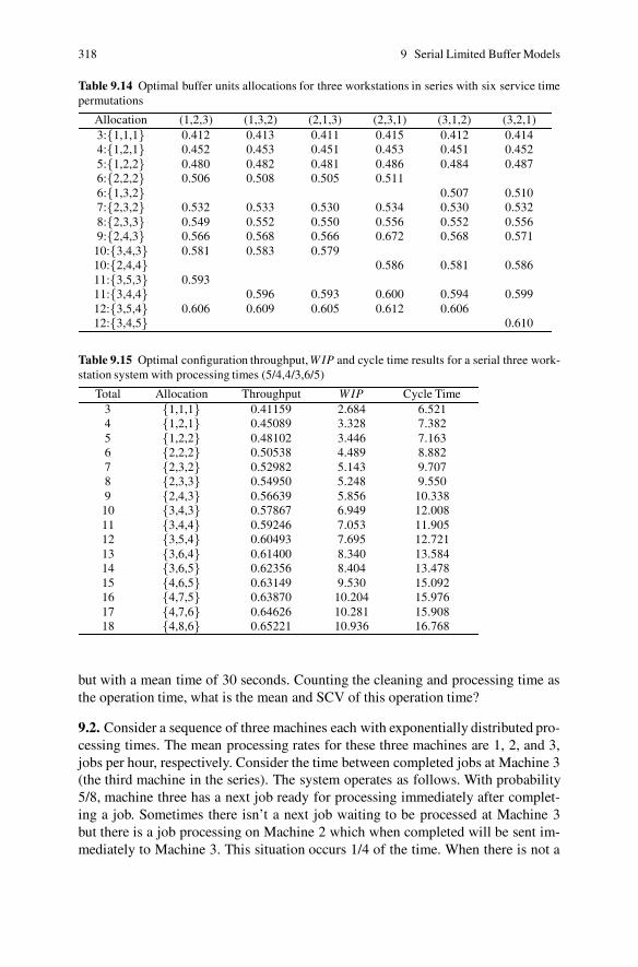
318 9 Serial Limited Buffer Models
Table 9.14 Optimal buffer units allocations for three workstations in series with six service timepermutations
Allocation (1,2,3) (1,3,2) (2,1,3) (2,3,1) (3,1,2) (3,2,1)3:{1,1,1} 0.412 0.413 0.411 0.415 0.412 0.4144:{1,2,1} 0.452 0.453 0.451 0.453 0.451 0.4525:{1,2,2} 0.480 0.482 0.481 0.486 0.484 0.4876:{2,2,2} 0.506 0.508 0.505 0.5116:{1,3,2} 0.507 0.5107:{2,3,2} 0.532 0.533 0.530 0.534 0.530 0.5328:{2,3,3} 0.549 0.552 0.550 0.556 0.552 0.5569:{2,4,3} 0.566 0.568 0.566 0.672 0.568 0.571
10:{3,4,3} 0.581 0.583 0.57910:{2,4,4} 0.586 0.581 0.58611:{3,5,3} 0.59311:{3,4,4} 0.596 0.593 0.600 0.594 0.59912:{3,5,4} 0.606 0.609 0.605 0.612 0.60612:{3,4,5} 0.610
Table 9.15 Optimal configuration throughput,W IP and cycle time results for a serial three work-station system with processing times (5/4,4/3,6/5)
Total Allocation Throughput W IP Cycle Time3 {1,1,1} 0.41159 2.684 6.5214 {1,2,1} 0.45089 3.328 7.3825 {1,2,2} 0.48102 3.446 7.1636 {2,2,2} 0.50538 4.489 8.8827 {2,3,2} 0.52982 5.143 9.7078 {2,3,3} 0.54950 5.248 9.5509 {2,4,3} 0.56639 5.856 10.33810 {3,4,3} 0.57867 6.949 12.00811 {3,4,4} 0.59246 7.053 11.90512 {3,5,4} 0.60493 7.695 12.72113 {3,6,4} 0.61400 8.340 13.58414 {3,6,5} 0.62356 8.404 13.47815 {4,6,5} 0.63149 9.530 15.09216 {4,7,5} 0.63870 10.204 15.97617 {4,7,6} 0.64626 10.281 15.90818 {4,8,6} 0.65221 10.936 16.768
but with a mean time of 30 seconds. Counting the cleaning and processing time asthe operation time, what is the mean and SCV of this operation time?
9.2. Consider a sequence of three machines each with exponentially distributed pro-cessing times. The mean processing rates for these three machines are 1, 2, and 3,jobs per hour, respectively. Consider the time between completed jobs at Machine 3(the third machine in the series). The system operates as follows. With probability5/8, machine three has a next job ready for processing immediately after complet-ing a job. Sometimes there isn’t a next job waiting to be processed at Machine 3but there is a job processing on Machine 2 which when completed will be sent im-mediately to Machine 3. This situation occurs 1/4 of the time. When there is not a
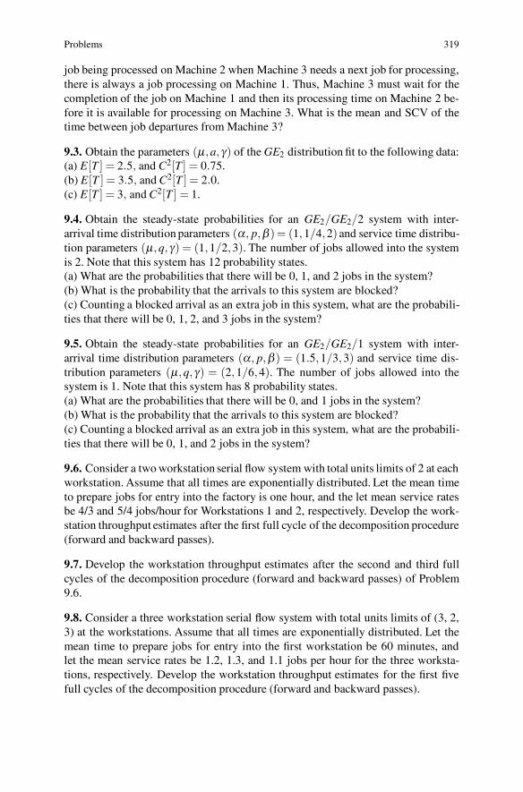
Problems 319
job being processed on Machine 2 when Machine 3 needs a next job for processing,there is always a job processing on Machine 1. Thus, Machine 3 must wait for thecompletion of the job on Machine 1 and then its processing time on Machine 2 be-fore it is available for processing on Machine 3. What is the mean and SCV of thetime between job departures from Machine 3?
9.3. Obtain the parameters (μ,a, γ) of the GE2 distribution fit to the following data:(a) E[T ] = 2.5, and C2[T ] = 0.75.(b) E[T ] = 3.5, and C2[T ] = 2.0.(c) E[T ] = 3, and C2[T ] = 1.
9.4. Obtain the steady-state probabilities for an GE2/GE2/2 system with inter-arrival time distribution parameters (α, p,β )= (1,1/4,2) and service time distribu-tion parameters (μ,q, γ) = (1,1/2,3). The number of jobs allowed into the systemis 2. Note that this system has 12 probability states.(a) What are the probabilities that there will be 0, 1, and 2 jobs in the system?(b) What is the probability that the arrivals to this system are blocked?(c) Counting a blocked arrival as an extra job in this system, what are the probabili-ties that there will be 0, 1, 2, and 3 jobs in the system?
9.5. Obtain the steady-state probabilities for an GE2/GE2/1 system with inter-arrival time distribution parameters (α, p,β ) = (1.5,1/3,3) and service time dis-tribution parameters (μ,q, γ) = (2,1/6,4). The number of jobs allowed into thesystem is 1. Note that this system has 8 probability states.(a) What are the probabilities that there will be 0, and 1 jobs in the system?(b) What is the probability that the arrivals to this system are blocked?(c) Counting a blocked arrival as an extra job in this system, what are the probabili-ties that there will be 0, 1, and 2 jobs in the system?
9.6. Consider a two workstation serial flow system with total units limits of 2 at eachworkstation. Assume that all times are exponentially distributed. Let the mean timeto prepare jobs for entry into the factory is one hour, and the let mean service ratesbe 4/3 and 5/4 jobs/hour for Workstations 1 and 2, respectively. Develop the work-station throughput estimates after the first full cycle of the decomposition procedure(forward and backward passes).
9.7. Develop the workstation throughput estimates after the second and third fullcycles of the decomposition procedure (forward and backward passes) of Problem9.6.
9.8. Consider a three workstation serial flow system with total units limits of (3, 2,3) at the workstations. Assume that all times are exponentially distributed. Let themean time to prepare jobs for entry into the first workstation be 60 minutes, andlet the mean service rates be 1.2, 1.3, and 1.1 jobs per hour for the three worksta-tions, respectively. Develop the workstation throughput estimates for the first fivefull cycles of the decomposition procedure (forward and backward passes).
320 9 Serial Limited Buffer Models
References
1. Altiok, T. (1996). Performance Analysis of Manufacturing Systems. Springer-Verlag, N.Y.2. Altiok, T., and Stidham, Jr., S. (1983). The Allocation of Interstage Buffer Capacities in Pro-
duction Lines. IIE Transactions, 15:292–299.3. Arrts, E., and Lenstra, J.K., editors (1997). Local Search in CombinatorialOptimization. John
Wiley & Sons.4. Dallery, Y., and Frein, Y. (1993). On Decomposition Methods for Tandem Queueing Net-
works with Blocking. Operations Research, 41:386–399.5. Deuermeyer, B. L., Curry, G.L., Duchowski, A.D., and Venkatesh, S. (1997). An Automatic
Approach to Deadlock Detection and Resolution in Discrete Simulation Systems. INFORMSJournal on Computing, 9:195–205.
6. Glover, F., and Luguna, M. (1997). Tabu Search, Kluwer Academic Publishers.7. Hillier, F.S., and So, K.C. (1991). The Effect of the Coefficient of Variation of Operation
Times on the Allocation of Storage Space in Production Line Systems. IIE Transactions,23:198–206.
8. Hillier, F.S., and So, K.C. (1995). On the Optimal Design of Tandem Queueing Systems withFinite Buffers. Queueing Systems, 21:245–266.
9. Jun, K.P., and Perros, H.G. (1988). Approximate Analysis of Arbitrary Configurations ofQueueing Networks with Blocking and Deadlock. Queueing Networks with Blocking: Pro-ceedings of the First International Conference Workshop, Raleigh, NC, pp. 259–279.
10. Lee, H. S., and Pollock, S.M. (1990). Approximation Analysis of Open Acyclic ExponentialQueueing Networks With Blocking. Operations Research, 38:1123–1134.
11. Neuts, M.F. (1981). Matrix-Geometric Solution in Stochastic Models, Johns Hopkins Univer-sity Press, Baltimore.
12. Papadopoulos, H.T., Heavey, C., and Browne, J. (1993). Queueing Theory in ManufacturingSystems Analysis and Design. Chapman & Hall, London.
13. Perros, H. (1994). Queueing Networks with Blocking. Oxford University Press, N. Y.14. Smith, J.M., and Daskalaki, S. (1988). Buffer Space Allocation in Automated Assembly
Lines. Operations Research, 36:343–358.15. Spinellis, D., Papadopoulos, C. and Smith, J.M. (2000). Large Production Line Optimization
using Simulated Annealing. Int. J. Prod. Res., 38:509–541.16. Venkatesh, S., Smith, J., Deuermeyer, B.L., and Curry, G.L. (1998). Deadlock Detection and
Resolution for Discrete-Event Simulation: Multiple-Unit Seizes. IIE Transactions, 30:201–216.
Glossary
availability The long-run average fraction of time that the processor is availablefor processing jobs, denoted by a (p. 113).
cellular manufacturing The concept of organizing the factory into sub-factorieswith the capability to produce a technology group (p. 177).
closed queueing network A network of queues in which no arrivals are possiblefrom outside the network and no jobs within the network can leave (p. 242).
coefficient of variation (CV) The standard deviation divided by the mean; usuallyrestricted to positive random variables (p. 13).
conditional probability The probability of event A given B is Pr(A∩B)/Pr(B) ifPr(B) �= 0 (p. 2). Also used for random variables when information of one randomvariable is known and the distribution of the other random variable is desired (p. 26).
CONWIP A production control strategy in which a constant level of work-in-process is maintained within the facility and thus a form of pull-release controlis used for jobs entering the system but not at each workstation (p. 241).
correlation coefficient The covariance of two random variables divided by theproduct of the two standard deviations (p. 29).
covariance The expected value of the product of the difference of one randomvariable and its mean multiplied by the difference of the second random variableand its mean (p. 29).
cumulative distribution function (CDF) A function associated with a randomvariable giving the probability that the random variable is less than or equal to thespecified value (p. 5).
cycle time The time that a job spends within a system. The average cycle time isdenoted by CT (p. 46).
321

322 Glossary
effective arrival rate The rate at which jobs enter the system, often denoted by λe.Notice that λ often represents the rate that jobs come to the system and λe representsthe rate that jobs are allowed into the system (p. 73).
effective processing time The time duration from when a job first has control ofa processor or machine until the time at which the job releases the processor ormachine so that it is available to begin work on another job; thus, it might includeactual processing time plus a setup time or repair time in case of processor failure(p. 113).
event A subset from the sample space, or a set of outcomes (p. 1).
expected value The expected value of a discrete random variable is the sum overall possible values of the random variable times the probability that the value willoccur; with continuous random variables, the integral replaces the sum (p. 10).
group technology The analysis of processing operations with the goal of deter-mining the similarity of the processing functions and, hence, the grouping of theassociated parts for production purposes (p. 177).
independence Random variables are independent if knowledge of the value of onerandom variable does not provide any information in predicting the value of theother random variables (p. 7).
indicator function The indicator function for integers is a matrix with the valueof 1 on the diagonal and 0 off the diagonal. If the matrix is square, it is an identitymatrix (p. 170).
job type Jobs with different routes or different processing characteristics are saidto be of different job types (p. 48).
joint distribution function The distribution function associated with two or morerandom variables (p. 23).
kanban A production control strategy in which a maximum limit on work-in-process at each workstation is maintained and thus a form of pull-release controlis used at each workstation (p. 281).
marginal distribution function The distribution function associated with one ran-dom variable, usually derived from a joint distribution function (p. 24).
mean The mean of a random variable is its expected value (p. 11).
memoryless property The lack of memory property is usually associated with arandom variable that denotes the time at which an event occurs and the propertyimplies that the probability of when the event will occur is the same as the condi-tional probability of when the event occurs given that the event has not yet occurred(p. 17).
mixture of random variables The probabilistic selection of one random variableamong a group of independent random variables (p. 34).
Glossary 323
outcome An element of the sample space (p. 1).
offered workload See workload.
Poisson process A renewal process formed by the sum of exponential random vari-ables (pp. 16 and 134).
probability density function (pdf) A function associated with a continuous ran-dom variable such that a probability that the random variable is between to valuesequals the integral of the function between those values (p. 6).
probability mass function (pmf) A function associated with a discrete randomvariable giving the probability that the random variable equals the independent vari-able (p. 6).
probability space A three-tuple (Ω ,F ,Pr) where Ω is a sample space, F is acollection of events from the sample space, and Pr is a probability measure thatassigns a number to each event contained in F (p. 1).
pull A general control strategy applied to a system that has a limit applied to itswork-in-process. After the maximum number of jobs are within the system, furtherjobs are allowed into the system only when they are “pulled” into the system byother jobs departing from the system (pp. 241 and 267).
push The standard operating assumption for open queueing networks in which jobsenter the system whenever they arrive to the system or according to a scheduleindependent of the system status (pp. 241 and 267).
random variable A function that assigns a real number to each outcome in thesample space (p. 4).
renewal process A process formed by the sum of nonnegative random variablesthat are independent and identically distributed (p. 134).
routes The sequence of processing steps for a job (p. 48).
routing matrix A matrix of probabilities, P = (pi j), where pi, j is the probabilitythat an arbitrary job leaving Workstation i will be routed directly to Workstation j(p. 139).
sample space A set consisting of all possible outcomes (p. 1).
squared coefficient of variation (SCV) The variance divided by the square of themean value (usually restricted to positive random variables) (p. 13).
standard deviation The square root of the variance (p. 11).
step-wise routing matrix A routing matrix indicating the probability of movingfrom processing step to processing step instead of from workstation to workstation(p. 169).
switching rule The probabilities that indicate the probabilistic branching for jobsas they depart from one workstation and get routed to another (p. 139).

324 Glossary
throughput rate The number of completed jobs leaving the system per unit oftime. The throughput rate averaged over many jobs is denoted by th (p. 47).
variance The variance of a random variable is the expected value of the squareddifference between the random variable and its mean. Equivalently, it is the secondmoment minus the square of the mean (p. 11).
work-in-process The number of jobs within a system that are either undergoingprocessing or waiting in a queue for processing. The average work-in-process isdenoted by W IP (p. 46).
workload The total amount of work that is required of a workstation per unit oftime and is determined by the sum of the total arrival rate (per time unit) for eachproduct type multiplied by its associated mean processing time (in time units con-sistent with the arrival rate) (p. 159).
workstation A collection of one or more identical machines or resources (p. 47).
workstation mapping function Gives the workstation assigned to each step of theproduction plan (p. 168).

Index
algorithmmarginal distribution analysis
exponential, 249non-exponential, 267
mean value analysisExcel, 272exponential, 247multi-product, 257, 260, 263non-exponential, 253
arrival processclosed networks, 246, 256merging streams, 134multiple product, 160random branching, 219SCV for merging streams, 141total arrival rate, 140
asymptotic approximation, 134
balance equations, 73batch models
batch move, 198batch network example, 222batch type service, 209departure SCV, 220setup reduction, 206workstations after batch service, 213
Bernoulli, 14Bernoulli decomposition, 136binomial, 14Bortkiewicz, L.V., 16breakdowns, 113
cellular manufacturing, 177central limit theorem, 22Chebyshev, P.L., 10closed queueing network, 241, 255coefficient of variation, 13
conditional expectation, 33conditional probability
definition, 2probability density function, 26probability mass function, 25
confidence interval, 100convolution, 8, 9CONWIP, 241correlation coefficient, 28covariance, 28Coxian distribution, 89, 282cumulative distribution function
definition, 5joint, 23properties, 5
cycle time, 46
de Moivre, A., 21decomposition, 128, 282departure process, 125
batch moves, 204batch service, 211, 220batch setups, 209deterministic routings, 175splitting streams, 135, 214
deterministic routing, 174diagrams, 73distributions
Bernoulli, 14binomial, 14continuous uniform, 16Coxian, 89discrete uniform, 13Erlang, 18exponential, 17
memoryless property, 17, 85gamma, 19
325

326 Index
generalized Erlang (GE), 89, 285geometric, 15mixture of generalized Erlangs (MGE), 286normal, 21Poisson, 15Weibull, 20Weibull parameters, 36
effective arrival rate, 73effective processing time, 113Erlang, 18Erlang models, 85, 87Excel
equation generation, 150gamma function, 35goal seek, 36matrix inverse, 97mean value analysis, 272simulation, 62, 98, 150t-statistic, 100Weibull parameters, 36
expected valuedefinition, 10property, 11
exponential, 17
factory modelsdeterministic, 54deterministic routing, 174general structure, 133multiple product networks, 159processing step paradigm, 167serial workstations, 125single workstation, 69various forms of batching, 197
factory performancegeneral networks, 138
factory performance modelingstochastic, 125
finite queues, 285flow shop, 48
gamma distribution, 19gamma function, 19, 35Gauss, K., 21general distribution models, 93, 95general service models, 91, 253generalized Erlang (GE), 89, 285generator, 286, 290geometric, 15glossary, 321Gosset, W.S., 16group technology, 177
i.i.d., 32independence, 7, 28
job shop, 48job type, 48joint
cumulative distribution function, 23probability density function, 25probability mass function, 23
just-in-time, 241
kanban, 241, 267, 281Kendall notation, 76
marginalprobability density function, 25probability mass function, 24
marginal distribution analysisexponential, 249non-exponential, 267
Markovian routing, 136matrix inverse, 97mean, 11mean value analysis, 242
Excel, 272exponential, 245, 247multi-product, 257, 260, 263, 267multi-servers, 249, 267non-exponential, 253
memoryless property, 17, 85merging streams, 133mixture of generalized Erlangs (MGE), 286mixtures of random variables, 34multiple product networks, 159multiple servers, 249, 267multiple streams, 139multivariate distributions, 23
network, 125, 222network approximations, 138non-identical servers, 81nonserial network models, 133, 139normal, 21
offered workload, 159open systems
multiple streams, 139single product, 145
operator-machine interactions, 116
performance measurescycle time, 46throughput rate, 47work-in-process, 46
phase-type models, 89
Index 327
Poisson, 15Pollaczek and Khintchine formula, 91probability, 1
conditional, 2measure, 1properties, 1space, 1
probability density functionconditional, 26definition, 6joint pdf, 25marginal pdf, 25
probability mass functionconditional, 25definition, 6joint, 23marginal, 24
processing step, 48processing step paradigm, 167processing time variability, 111pull, 241, 267push, 241, 267
queueing modelsErlang-2/M/1/3, 87G/G/1 approximation, 93G/G/c approximation, 95GE-2/Erlang-2/1/3, 89limited buffer, 285M/Erlang-2/1/3, 86M/G/1, 91M/M/1, 77, 78
cycle time, 80M/M/1/n, 69non-identical servers, 81Pollaczek and Khintchine formula, 91
queueing network modelsclosed, 241open, 125, 133
queueing notation, 76
random sized batches, 216–218random variable
definition, 4random variables
convolution, 8correlation coefficient, 29fixed sum, 31independent, 7, 28mixture, 34nonnegative, 9random sum, 33
re-entrant flow, 48relative arrival rates, 245
renewal process, 134repairs, 113routing, 48routing matrix, 139
sample space, 1scale parameter, 19, 20serial network model, 128, 213, 293setups, 206shape parameter, 19, 20simulation, 62, 98, 150single server, 90skewness, 23solutions to linear systems, 97splitting streams, 135squared coefficient of variation, 13
departure SCV, 127service SCV, 163
standard deviation, 10steady-state, 69, 73sums of random variables
fixed, 31random, 33
switching probabilities, 164switching rule, 139
throughput rate, 47two-node systems, 284
uniform, continuous, 16uniform, discrete, 13utilization, 84
multiple products, 162single product, 92
variancecoefficient of variation, 13definition, 11property, 12
Venn diagrams, 2
Weibull distribution, 20, 36Weibull, W., 20WIP
formula, 52limits
constant, 241kanban, 281
production controlpull, 241push, 241
work-in-process, 46workload, 159, 162workstations, 46, 47