1. University of California, San Diego

2. Tsinghua University

An Algorithmic Framework of

Large-Scale Circuit Simulation Using

Exponential Integrators

Hao Zhuang1, Wenjian Yu2, Ilgweon Kang1, Xinan

Wang1, and Chung-Kuan Cheng1

2

Outline

• Motivation & Contributions

• Background of time-domain circuit simulation

• Our algorithmic framework

• Exponential integrators

• Invert Krylov subspace method

• Experimental results

• Conclusions & future directions

Motivation • SPICE

– critical to wide ranges of IC

• Modern IC

– billions of transistors

– complex interconnects

• Requirement:

– new structures e.g., FinFET, 3D

– strong coupled

– post-layout effects

– capability & accuracy

• Simulation runtime

– Long or ∞

3

From Dick Sites, “Datacenter

Computers modern challenges in CPU

design” Google Inc. 2015 & Intel i7

From Synopsys Inc. Issue 3, 2012

Technology Update FinFET: The Promises

and the Challenges

• Target of matrix factorization:

conductance matrix 𝐺 ONLY Less expensive

4

Contributions • Exponential Integration

Stable, Explicit No Newton-Raphson

• Handling tasks (even when traditional schemes

FAIL)

• large-scale, strong coupled, post-layout

A promising framework

Basic & BENR as An Example (1)

• Differential Equations

• BE: Backward Euler

5

capacitance

(/inductance)

conductance

(/incidence)

time step

input

nonlinear devices dynamics

Basic & BENR as An Example (2)

• NR: Newton-Raphson

• BENR: Backward Euler + Newton-Raphson

iterations

6

Jacobian matrix

Basic & BENR as An Example (3)

• NR: Newton-Raphson

• BENR: Backward Euler + Newton-Raphson

iterations

7

Jacobian matrix

capacitance

matrix

Matrix Exponential Method

• Our previous attempt [Weng12]

where

8

Matrix Exponential Method

• Our previous attempt [Weng12]

where

• It also uses NR

The Jacobian matrix

9

capacitance matrix

10

𝐶, 𝐺 matrices from FreeCPU [Zhang, Yu TCAD 2013]

nnz: non-zero terms

𝐺 𝐶

Matrices from a Post-Layout Case

11 𝑙𝑢(𝐶)

𝐶, 𝐺 matrices

𝐺 𝐶

𝐿 𝑈

Matrices from a Post-Layout Case

12

𝑙𝑢(𝐶

𝑕+ 𝐺)

𝐶, 𝐺 matrices

𝐺 𝐶 𝐿 𝑈

Matrices from a Post-Layout Case

13

Matrices from a Post-Layout Case

𝐿 and 𝑈 of 𝑙𝑢(𝐶)

𝐿 and 𝑈 of 𝑙𝑢(𝐶

ℎ+ 𝐺)

𝑙𝑢(𝐺)

𝐿 𝑈

𝐶, 𝐺 matrices

14

𝐿 and 𝑈 of 𝑙𝑢(𝐶

ℎ+ 𝐺)

𝐿 and 𝑈 of 𝑙𝑢(𝐺)

In this example, 𝑙𝑢(𝐺) • contains less nnz (~10%)

&

• less complicated nnz

distributions

Matrices from a Post-Layout Case

• Traditional methods are

all challenged by 𝐶,

when 𝐶 is complicated,

• Two techniques:

– ER: Exponential Rosenbrock Formulation

– Invert Krylov subspace to compute 𝑒𝐽𝑣

• Computational advantages

– Simple matrix factorization target: exploit the

feature of 𝑙𝑢(𝐺)

– Stable explicit method to solve circuit system

15

Our proposed framework

ER: Exponential Rosenbrock

Start from

𝑑𝑥 𝑡

𝑑𝑡= 𝑔 (𝑥 , 𝑢, 𝑡)

• The next time step solution [Hochbruck, et. al. SIAM09]

𝑥 𝑘+1 = 𝑥 𝑘 + 𝑕𝑘𝜙1 𝑕𝑘𝐽𝑘 𝑔 (𝑥 𝑘 , 𝑢, 𝑡𝑘) + 𝑕𝑘2 𝜙2 𝑕𝑘𝐽𝑘 𝑏k

where 𝐽𝑘 = 𝜕𝑔 /𝜕𝑥 , 𝑏𝑘 = 𝜕𝑔 /𝜕𝑡

𝜙1 𝑕𝑘𝐽𝑘 = (𝑒ℎ𝑘𝐽𝑘−𝐼𝑛)/𝑕𝑘𝐽𝑘

𝜙2 𝑕𝑘𝐽𝑘 = (𝑒ℎ𝑘𝐽𝑘−𝐼𝑛)/𝑕𝑘2𝐽𝑘

2 − 𝐼𝑛/𝑕𝑘𝐽𝑘

16

Exponential Integrators:

Proved to be Stable, Explicit, High-Order Accuracy for ODE

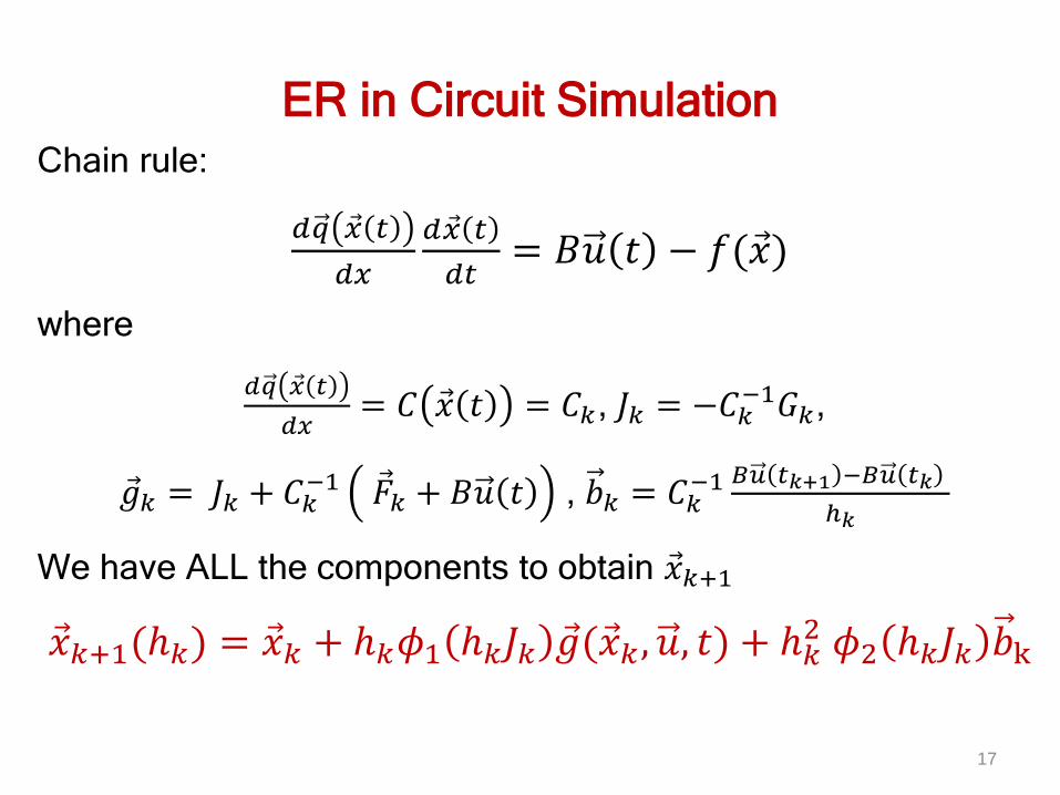
ER in Circuit Simulation

Chain rule:

𝑑𝑞 𝑥 𝑡

𝑑𝑥

𝑑𝑥 𝑡

𝑑𝑡= 𝐵𝑢 𝑡 − 𝑓(𝑥 )

where

𝑑𝑞 𝑥 𝑡

𝑑𝑥= 𝐶 𝑥 𝑡 = 𝐶𝑘, 𝐽𝑘 = −𝐶𝑘

−1𝐺𝑘,

𝑔 𝑘 = 𝐽𝑘 + 𝐶𝑘−1 𝐹 𝑘 + 𝐵𝑢 𝑡 , 𝑏𝑘 = 𝐶𝑘

−1 𝐵𝑢 𝑡𝑘+1 −𝐵𝑢 𝑡𝑘

ℎ𝑘

We have ALL the components to obtain 𝑥 𝑘+1

𝑥 𝑘+1(𝑕𝑘) = 𝑥 𝑘 + 𝑕𝑘𝜙1 𝑕𝑘𝐽𝑘 𝑔 (𝑥 𝑘 , 𝑢, 𝑡) + 𝑕𝑘2 𝜙2 𝑕𝑘𝐽𝑘 𝑏k

17

Local Nonlinear Error Control

The local nonlinear error estimator [Caliari09]

𝑒𝑟𝑟 𝑥 𝑘+1, 𝑥 𝑘 = 𝜙1 𝑕𝑘𝐽𝑘 𝐶𝑘−1Δ𝐹 𝑘

where Δ𝐹 𝑘 = 𝐹 𝑥 𝑘+1 − 𝐹 (𝑥 𝑘)

18

ER-C: ER with Correction Term

Reuse Δ𝐹 𝑘 to improve the accuracy by padding

the extra term

𝐷𝑘 = 𝛾𝑕𝑘𝜙2 𝑕𝑘𝐽𝑘 𝐶𝑘−1Δ𝐹 𝑘

The further corrected solution is

𝑥 𝑘+1,𝑐 = 𝑥 𝑘+1 − 𝐷𝑘

Krylov Method for MEVP 𝑒𝐽𝑣 • 𝑒𝐽𝑣: Matrix Exponential and Vector Product

(MEVP) via standard Krylov subspace [Weng12]

𝐾𝑚 𝐽, 𝑣 ≔ 𝑠𝑝𝑎𝑛 𝑣 , 𝐽𝑣 , 𝐽2𝑣 , … , 𝐽𝑚−1𝑣

– Arnoldi process and Matrix reduction:

𝐽𝑉𝑚 = 𝑉𝑚𝐻𝑚 + 𝑕𝑚+1,𝑚𝑣 𝑚+1𝑒 𝑚T

• MEVP is computed by

𝑒𝐽𝑣 ≈ 𝑣 2𝑉𝑚 𝑒𝐻𝑚𝑒 1

• Explicit feature: time stepping only by scaling 𝐻𝑚

with h,

𝑒ℎ𝐽𝑣 ≈ 𝑣 2𝑉𝑚 𝑒ℎ𝐻𝑚𝑒 1

19

20

Standard Krylov subspace

Im

Re 0

“like” these eigenvalues

Eigenvalues of J: small magnitude of Re

Eigenvalues of J: large magnitude of Re

(a) Standard Krylov Basis [Weng12]

𝐾𝑚 𝐽, 𝑣 ≔ 𝑠𝑝𝑎𝑛 𝑣 , 𝐽𝑣 , 𝐽2𝑣 , … , 𝐽𝑚−1𝑣

spectrum of

𝐽 = −𝑪−𝟏𝑮

21

Standard Krylov subspace

Im

Re 0

• these eigenvalues

defines the major

dynamical behavior

• demand more bases to

characterize

Eigenvalues of J: small magnitude of Re

Eigenvalues of J: large magnitude of Re

(a) Standard Krylov Basis [Weng12]

𝐾𝑚 𝐽, 𝑣 ≔ 𝑠𝑝𝑎𝑛 𝑣 , 𝐽𝑣 , 𝐽2𝑣 , … , 𝐽𝑚−1𝑣

spectrum of

𝐽 = −𝑪−𝟏𝑮

22

Im

Re

Im

Re 0 0

Invert Krylov subspace method captures

“important” eigenvalues in the original spectrum

Eigenvalues of J: small magnitude of Re

Eigenvalues of J: large magnitude of Re

Invert Krylov subspace

Invert Krylov Basis [Zhuang, et. al. DAC14]

𝐾𝑚 𝐽−1, 𝑣 ≔ 𝑠𝑝𝑎𝑛 𝑣 , 𝐽−1𝑣 , 𝐽−2 𝑣 , … , 𝐽−𝑚+1𝑣

spectrum of 𝐽−1 spectrum of 𝐽

Simple Matrix Fct. Taget

23

Invert Krylov Subspace approach transfers

𝐽 = −𝐶−1𝐺 𝐽−1= −𝐺−1𝐶

At each iteration, we

generate invert

Krylov subspace

𝑉𝑚 = 𝑣 1, 𝑣 2, ⋯ , 𝑣 𝑚

by solving

−𝑮𝒘 = 𝑪𝒗𝒊−𝟏

24

Overall Framework

ER-C: further

improve the solution

• No Newton-Raphson

• Build upon exponential

integrators

• explicit method for

DAE solver

• adjust error by step

size control

Experimental Results

• Implemented in MATLAB2013a & C/C++ (GCC

4.7.3)

– Opensource BSIM3 device model with C

– MATLAB Executable (MEX) external interface

between device evaluation and matrix solvers

• Linux workstation

– Intel CPU i7 3.4GHZ

– 32GB memory.

– Utilize single thread mode.

25

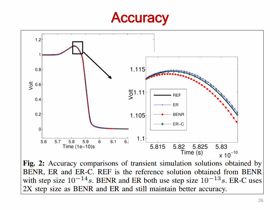
Accuracy

26

27

Runtime Performance • #Dev.: the number of devices.

• nnzC & nnzG: the number of non-zero

elements in linear C and G.

• #step: the number of steps for transient

simulation;

For each time step,

• #NRa: the average NR iterations

• #ma: the average dimension of invert

Krylov subspace

• RT(s): the runtime.

• SP: the runtime speedup Test circuits

28

Conclusions and Future Directions

Accelerate SPICE-level time-domain simulation

• Exponential Integrators

• Stable explicit formulation

• 𝑒𝐽𝑣 w/ invert Krylov Subspace & Less expensive matrix factorizations.

• Handling tasks even when traditional methods fail.

Future directions:

• parallelism, can be accelerated further by multicore/many-core computing systems.

• many derivatives & tools can be built upon.

Thanks and Q&A

29