Wave diffraction

$Page 1: Wave diffraction$
Waves and Diffraction in SolidsSolution to Chapter Problems

Bruce M. ClemensStanford University

Winter 2002

ii

Copyright 2002 Bruce M. Clemens

Contents

1 Waves and Fourier Analysis 1

2 Group Velocity and Dispersion 9

3 Physical Examples of Waves 11

4 Wave Intensity and Polarization 15

5 Maxwell’s Equations: Light Waves 17

6 X-Ray Scattering From Electrons and Atoms 21

7 X-Ray Scattering From Crystals 23

8 Experimental Methods of Diffraction 43

9 Phonons: Lattice Vibrations and Modes 61

10 Quantum Mechanics Review 69

11 Quantized Phonon Behavior 77

12 Statistical Mechanics 81

iii

iv CONTENTS

Chapter 1

Waves and Fourier Analysis

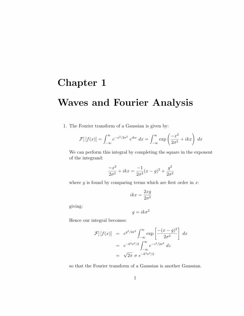
1. The Fourier transform of a Gaussian is given by:

F ] [f(x)] =∫ ∞−∞

e−x2/2σ2

eikx dx =∫ ∞−∞

exp

(−x2

2σ2+ ikx

)dx

We can perform this integral by completing the square in the exponentof the integrand:

−x2

2σ2+ ikx =

−1

2σ2(x− g)2 +

g2

2σ2

where g is found by comparing terms which are first order in x:

ikx =2xg

2σ2

giving:g = ikσ2

Hence our integral becomes:

F ] [f(x)] = eg2/2σ2

∫ ∞−∞

exp

[−(x− g)2

2σ2

]dx

= e−k2σ2/2

∫ ∞−∞

e−z2/2σ2

dz

=√

2π σ e−k2σ2/2

so that the Fourier transform of a Gaussian is another Gaussian.

1

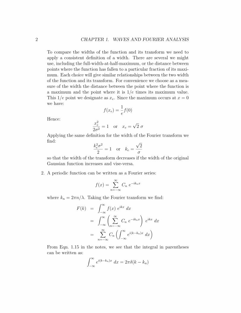
2 CHAPTER 1. WAVES AND FOURIER ANALYSIS

To compare the widths of the function and its transform we need toapply a consistent definition of a width. There are several we mightuse, including the full-width-at-half-maximum, or the distance betweenpoints where the function has fallen to a particular fraction of its maxi-mum. Each choice will give similar relationships between the two widthof the function and its transform. For convenience we choose as a mea-sure of the width the distance between the point where the function isa maximum and the point where it is 1/e times its maximum value.This 1/e point we designate as xe. Since the maximum occurs at x = 0we have:

f(xe) =1

ef(0)

Hence:x2e

2σ2= 1 or xe =

√2 σ

Applying the same definition for the width of the Fourier transform wefind:

k2eσ

2

2= 1 or ke =

√2

σso that the width of the transform decreases if the width of the originalGaussian function increases and vise-versa.

2. A periodic function can be written as a Fourier series:

f(x) =∞∑

n=−∞Cn e

−iknx

where kn = 2πn/λ. Taking the Fourier transform we find:

F (k) =∫ ∞−∞

f(x) eikx dx

=∫ ∞−∞

( ∞∑n=−∞

Cn e−iknx

)eikx dx

=∞∑

n=−∞Cn

(∫ ∞−∞

ei(k−kn)x dx)

From Eqn. 1.15 in the notes, we see that the integral in parenthesescan be written as: ∫ ∞

−∞ei(k−kn)x dx = 2πδ(k − kn)

3

Hence the Fourier transform is given by:

F (k) =∞∑

n=−∞2πCn δ(k − kn)

We see that the Fourier transform of a periodic function is non-zero onlyat k values corresponding to harmonic components of the periodicity.

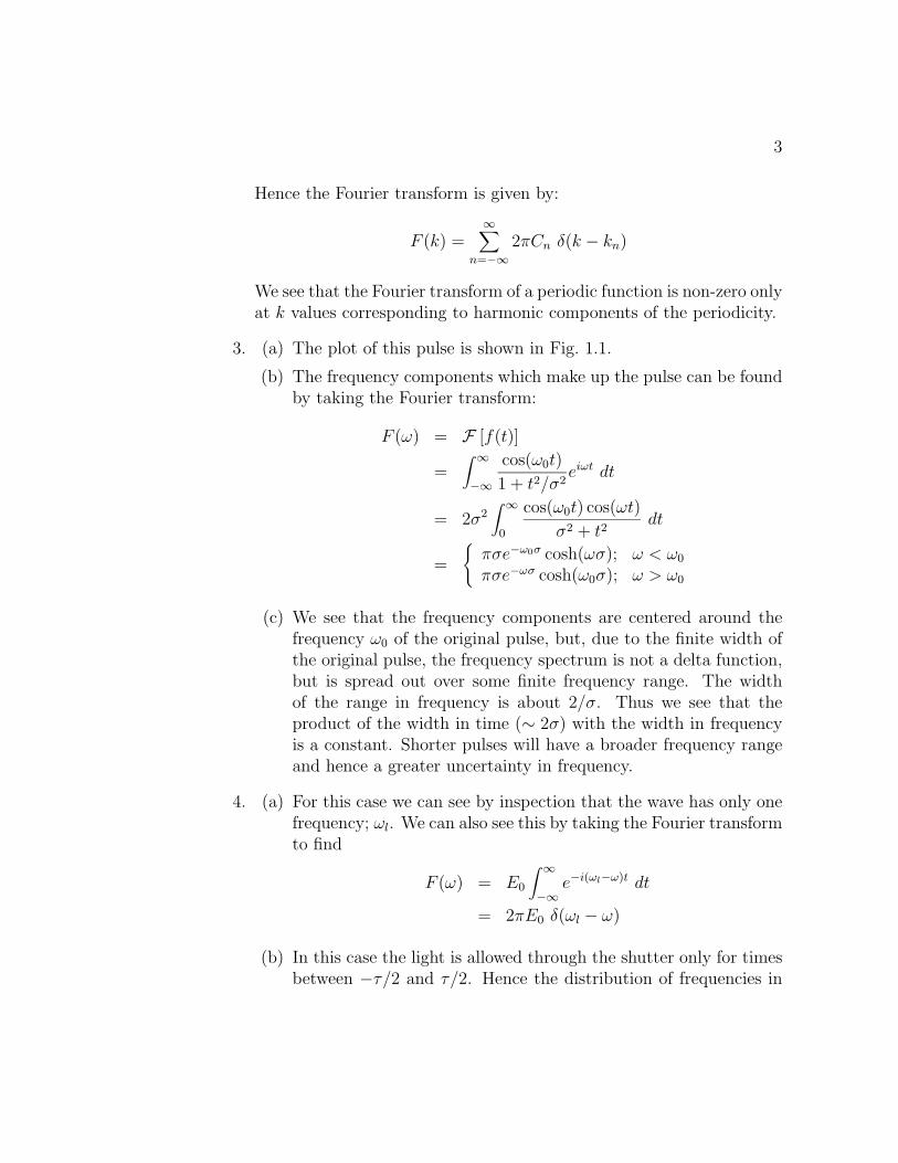
3. (a) The plot of this pulse is shown in Fig. 1.1.

(b) The frequency components which make up the pulse can be foundby taking the Fourier transform:

F (ω) = F [f(t)]

=∫ ∞−∞

cos(ω0t)

1 + t2/σ2eiωt dt

= 2σ2∫ ∞

0

cos(ω0t) cos(ωt)

σ2 + t2dt

=

{πσe−ω0σ cosh(ωσ); ω < ω0

πσe−ωσ cosh(ω0σ); ω > ω0

(c) We see that the frequency components are centered around thefrequency ω0 of the original pulse, but, due to the finite width ofthe original pulse, the frequency spectrum is not a delta function,but is spread out over some finite frequency range. The widthof the range in frequency is about 2/σ. Thus we see that theproduct of the width in time (∼ 2σ) with the width in frequencyis a constant. Shorter pulses will have a broader frequency rangeand hence a greater uncertainty in frequency.

4. (a) For this case we can see by inspection that the wave has only onefrequency; ωl. We can also see this by taking the Fourier transformto find

F (ω) = E0

∫ ∞−∞

e−i(ωl−ω)t dt

= 2πE0 δ(ωl − ω)

(b) In this case the light is allowed through the shutter only for timesbetween −τ/2 and τ/2. Hence the distribution of frequencies in


1.0

0.5

0.0

-0.5

f

-4 -2 0 2 4

t/σ

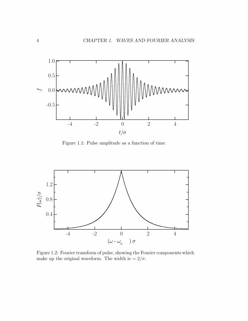
Figure 1.1: Pulse amplitude as a function of time.

1.2

0.8

0.4

F( ω

)/σ

-4 -2 0 2 4

(ω - ω ) σ

Figure 1.2: Fourier transform of pulse, showing the Fourier components whichmake up the original waveform. The width is ∼ 2/σ.

5

this pulse (still given by the Fourier transform) is now

F (ω) = E0

∫ τ/2

−τ/2e−i(ωl−ω)t dt

=E0

i(ωl − ω)

(ei(ωl−ω)τ/2 − e−i(ωl−ω)τ/2

)=

2E0

ωl − ωsin [(ωl − ω)τ/2]

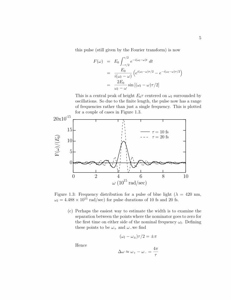
This is a central peak of height E0τ centered on ωl surrounded byoscillations. So due to the finite length, the pulse now has a rangeof frequencies rather than just a single frequency. This is plottedfor a couple of cases in Figure 1.3.

20x10-15

15

10

5

0

F( ω

)/( E

0)

1086420ω (10

15 rad/sec)

τ = 10 fs τ = 20 fs

Figure 1.3: Frequency distribution for a pulse of blue light (λ = 420 nm,ωl = 4.488× 1015 rad/sec) for pulse durations of 10 fs and 20 fs.

(c) Perhaps the easiest way to estimate the width is to examine theseparation between the points where the nominator goes to zero forthe first time on either side of the nominal frequency ωl. Definingthese points to be ω+ and ω−we find

(ωl − ω±)τ/2 = ±π

Hence

∆ω ≈ ω+ − ω− =4π

τ


So that the more we shrink the length in time with wider thespread in frequencies (and hence wavelengths). For the case shownin Figure 1.3 we have pulse widths of 10 fs and 20 fs. This corre-sponds to frequency ranges of 1.26×1015 rad/sec. and 0.628×1015

rad/sec. respectively. More interestingly this gives a spread inwavelengths given by

∆λ = 2πc

(1

ω−− 1

ω+

)

= 2πc

(∆ω

ω−ω+

)

≈ λl∆ω

ωl

This gives a wavelength spreads of 118 nm and 59 nm for the twopulse widths, both of which are appreciable fractions of the nomi-nal wavelength. So the shorter the light pulse the more uncertainits color.

5. (a) The Fourier transform of a delta function can be easily found byrecalling the sifting property of the delta function∫ ∞

−∞δ(x) f(x) dx = f(0)

Hence we find:i.

F (k) =∫ ∞−∞

δ(x) eikx dx = 1

ii.

F (k) =∫ ∞−∞

[δ(x− a) + δ(0) + δ(x+ a)] eikx dx

= eika + 1 + e−ika

= 1 + 2 cos ka

iii.

F (k) =∫ ∞−∞

[δ(x− 2a) + δ(x− a) + δ(0) + δ(x+ a) + δ(x+ 2a)] eikx dx

= ei2ka + eika + 1 + e−ika + e−i2ka

= 1 + 2 cos ka+ 2 cos 2ka

7

Sketches are shown in Figure 1.4

(b) The result for part i is a constant and so has no maxima. Thepeaks in parts ii and iii occure when ka = 2πn, or k = 2πn/a,which is the one-dimensional Bragg condition.

(c) For the infinite number of delta functions we can generalize to find

F (k) = 1 + 2∞∑n=1

cosnka

It is tricky to do so, but it can be shown that this is also an infinitestring of delta functions. One might deduce this by observing thatin going from the three delta functions in part ii to the five inpart iii the peaks sharpened and the background dropped. Henceextrapolating to an infinite number of delta functions will produceanother string of delta function peaks.

5

4

3

2

1

0

-1

F(k

)

-6 -4 -2 0 2 4 6

ka

i ii iii

Figure 1.4: Fourier transform of delta functions.

6. From an above problem we find that the frequency distribution in apulse of with τ is given by

∆ω =4π

τ


Hence the energy range is given by

∆E = h∆ω = h∆ν =2h

τ

Plugging in numbers we find

∆E =2 · 4.136× 10−15 eV sec

50× 10−15 sec= 0.17eV

Chapter 2

Group Velocity and Dispersion

1. The given equation can be solved for the dispersion relationship ω(k):

ω(k) =√ω2c + k2c2

The phase velocity is then:

vp =ω

k=

√ωck2

+ c2

and the group velocity is:

vg =dω

dk=

kc2√ω2c + k2c2

=kc2

ω=c2

vp

2. (a) The phase velocity is given by:

vp =ω

k=

√T

ρ+ αk2

=

√T

ρ

√1 +

αk2ρ

T

≈√T

ρ+αk2

2

√ρ

T

The qroup velocity is given by:

vg = vp + kdvpdk≈ vp + αk2

√ρ

T≈√T

ρ+

3αk2

2

√ρ

T

9

10 CHAPTER 2. GROUP VELOCITY AND DISPERSION

(b) For vibrations on a finite string the allowed wave numbers aregiven by:

kn =nπ

L

The allowed frequencies are:

ωn = vpkn ≈(nπ

L

)√T

ρ

[1 +

αρ

2T

(nπ

L

)2]

Thus the higher order (n > 1) frequencies are greater for thestiff wire than for the flexible wire. This gives the overtones ofthe instrument a distinctive sound. However, Dick Dale used stiffstrings because he wailed on them so hard that normal stringsbroke too often.

Chapter 3

Physical Examples of Waves

1. We know that the solutions for waves on a finite string of length L aregiven by:

ξn(x, t) = Bn sin (knx)

where the wavenumbers are restricted to maintain an integral numberof half wavelengths in the length of the string:

kn =nπ

L; λn =

2L

n

The allowed frequencies are just given by:

ωn = vkn =

√T

ρ

nπ

L

These solutions are just the Fourier components for a disturbance witha wavelength λ = 2L. We can find the magnitude of each harmoniccomponent by finding the corresponding Fourier coefficient for the ini-tial disturbance. Hence we find;

Bn =1

2L

∫ L

−Lf(x) sin

(2nπx

2L

)dx

=1

L

∫ L

0f(x) sin(knx) dx

=1

L

[∫ L/2

0

2bx

Lsin(knx) dx+

∫ L

L/2

(2b− 2bx

L

)sin(knx) dx

]

=4b

n2π2(−1)

n−12 ; n = 1, 3, 5, 7, . . .

11

12 CHAPTER 3. PHYSICAL EXAMPLES OF WAVES

So only the odd harmonics are present.

2. The transducer launches a wave which can be represented as

ξ = A ei(ωt−kz)

Hence the phase difference ∆φ for the wave at the source and transduceris just

∆φ = kL

The experimental observation that ∆φ is linear with frequency ω meansthat

kL = mω

Hence the velocity is given by

v =ω

k=L

m

Therefore we can find the modulus from

Y = v2ρ

=ρL2

m2

3. (a) The group velocity is:

vg =dω

dk=

{aη1/2 cos ka

2if 2nπ < ka

2≤ (2n+ 1)π

−aη1/2 cos ka2

if (2n+ 1)π < ka2≤ 2(n+ 1)π

(b) For small k, cos ka/2 ≈ 1, so the group velocity is:

vg ≈ ±aη1/2

where the sign is the sign of k. This is a constant, independentof k, so in this limit the phase and group velocities are equal, andthere is no dispersion.

(c) The group velocities will be zero when:

coska

2= 0

13

This will occur when:

ka

2=

(2n+ 1)π

2

or:

k =(2n+ 1)π

a

This is the Brillouin zone boundaries for this one-dimensional case.Hence the group velocity is zero when the wave number of thephonon satisfies the Bragg condition for diffraction.

14 CHAPTER 3. PHYSICAL EXAMPLES OF WAVES

Chapter 4

Wave Intensity andPolarization

1. (a) The power is proportional to the square of the wave:

P ∝ ξ2 = ξ20 cos2(kz − ωt) =

ξ20

2[1 + cos(2kz − 2ωt)]

So the power has a DC component with a magnitude of ξ20/2 and

an oscillatory part with a the same magnitude with twice thefrequency of the original wave.

(b) For this wave, in the z = 0 plane, the angle between the x-axisand a line connecting origin to the wave is given by:

tan θ =ξyξx

=sin(kz − ωt)cos(kz − ωt)

so that:

θ = kz − ωtAs t increases, θ decreases, so this is a left handed circularly po-larized wave. The power is again proportional to the square of theamplitude:

P ∝ ξ2 = ξ20

[cos2(kz − ωt) + sin2(kz − ωt)

]= ξ2

0

which means that the power is constant in time.

15

16 CHAPTER 4. WAVE INTENSITY AND POLARIZATION

2. (a) For t = 0, the points at which the two contributions to this waveare in-phase are given by the solutions to the equation:

k1xp = k2xp ± 2πn

where n is an integer. From this we find:

xp = ± 2πn

k1 − k2

(b) The times at which the contributions are in-phase at the positionx = 0 are found by solving:

ω(k1)tp = ω(k2)tp ± 2πn

This yields:

tp = ± 2πn

ω(k1)− ω(k2)

(c) For non-zero time, the positions where the contributions to thewave are in-phase are a function of time. We denote these posi-tions as xp(t). They can be found by solving the following equa-tion:

k1xp(t)− ω(k1)t = k2xp(t)− ω(k2)t± 2πn

Differentiating yields:

dxp(t)

dt=ω(k1)− ω(k2)

k1 − k2

Chapter 5

Maxwell’s Equations: LightWaves

1. (a) Substitution of the given solution into the wave equation gives:

−k2E = −ω2εrε0µrµ0E− iωµrµ0σE

dividing through by −ω2E yields:

k2

ω2=

1

v2p

= εrε0µrµ0 +iµrµ0σ

ω

(b) The square of the index of refraction is given by:

n2 =c2

v2p

=1

ε0µ0

(εrε0µrµ0 + i

µrµ0σ

ω

)= εrµr + i

µrσ

ε0ω(5.1)

The complex part of n can be found by writing:

n2 = Meiφ

where:

M =

√(εrµr)2 +

(µrσ

ε0ω

)2

and φ = arctan(

σ

εrε0ω

)Then n is just:

n =√n2 =

√M eiφ/2

17

18 CHAPTER 5. MAXWELL’S EQUATIONS: LIGHT WAVES

which has imaginary part:

=[n] = β =√M sin(

φ

2)

so that n is a complex quantity, and we can write:

n = n0 + iβ

where n, β ∈ R.

We can come up with an algebraic relationship between β and thematerials constants by writing n2 as:

n2 = (n0 + iβ)2 = n20 − β2 + 2in0β

comparing this with Eqn. 5.1 above, we equation the real andimaginary parts to find:

n20 − β2 = εrµr ; 2n0β =

µrσ

ε0ω

These two equations can be solved for β to find:

β =

√√√√−εrµr2

+1

2

√(εrµr)2 +

(µrσ

ε0ω

)2

As a side note, we can also solve for n0 to find:

n0 =

√√√√εrµr2

+1

2

√(εrµr)2 +

(µrσ

ε0ω

)2

Hence for nonconducting media, where σ = 0, we find:

β = 0 ; n = n0 =√εrµr

The relationship between the imaginary part of n and the absorp-tion coefficient is explored in the notes.

(c) From the notes we find:

α =2ωβ

c

which, combined with the above gives the desired result.

19

2. (a) The expression for light which is a right-circularly polarized waveat z = 0 and is traveling in the z direction through media withindices of refraction nx and ny for the x and y components of thefield respectively is given by:

E = E0

{cos

[ω(nxz

c− t

)]x− sin

[ω(nyz

c− t

)]y}

We see that in the x−y plane at z = 0, the vector E would have afixed length and rotate in a clockwise direction when viewed fromnegative to positive z.

(b) As we move through the media, we see that the phases of thetwo components change at a different rate due to the differencein refractive indices. The light will be linearly polarized when thetwo components are in phase. Since they were originally out ofphase by π/2 at z = 0, this will occur at a position zL whichsatisfies:

ω(nxzLc

)= ω

(nyzLc

)+π

2

Solving for zL we find:

zL =πc

2ω(nx − ny)

Inserting this position into our field we find:

E(zL, t) = E0

{cos

[ω(nxzLc− t

)]x− sin

[ω(nyzLc− t

)]y}

= E0

{cos

[nxπ

2(nx − ny)− ωt

]x

− sin

[nyπ

2(nx − ny)− ωt

]y

}

= E0

{cos

[nxπ

2(nx − ny)− ωt

]x

− sin

[nxπ

2(nx − ny)− π

2− ωt

]y

}

= cos

[nxπ

2(nx − ny)− ωt

](x+ y)

20 CHAPTER 5. MAXWELL’S EQUATIONS: LIGHT WAVES

If we plot E on the x−y plane at z = zL we find that it is linearlypolarized and oscillates with time along a line at 45◦ between the+x and +y axes.

Chapter 6

X-Ray Scattering FromElectrons and Atoms

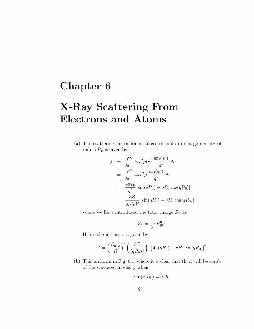
1. (a) The scattering factor for a sphere of uniform charge density ofradius R0 is given by:

f =∫ ∞

04πr2ρ(r)

sin(qr)

qrdr

=∫ R0

04πr2ρ0

sin(qr)

qrdr

=4πρ0

q3[sin(qR0)− qR0 cos(qR0)]

=3Z

(qR0)3[sin(qR0)− qR0 cos(qR0)]

where we have introduced the total charge Ze as:

Ze =4

3πR3

0ρ0

Hence the intensity is given by:

I =(E0reR

)2(

3Z

(qR0)3

)2

[sin(qR0)− qR0 cos(qR0)]2

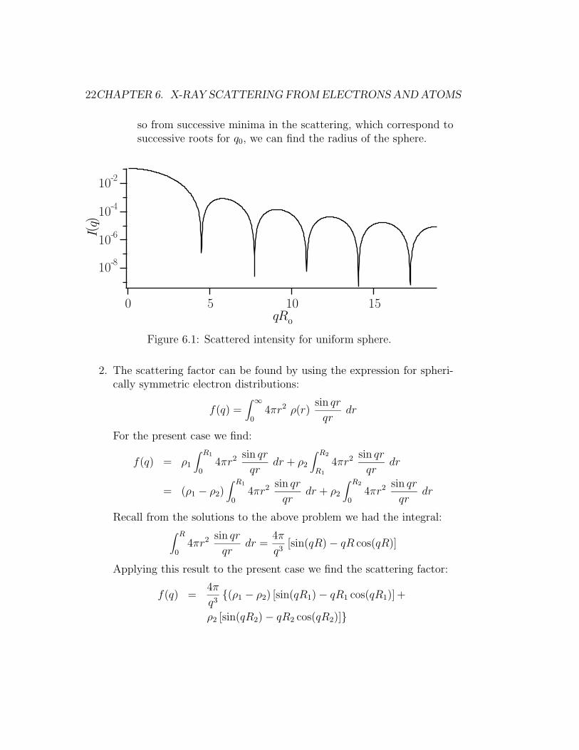
(b) This is shown in Fig. 6.1, where it is clear that there will be zero’sof the scattered intensity when:

tan(q0R0) = q0R0

21

10-8

10-6

10-4

10-2

I(q)

151050qR

22CHAPTER 6. X-RAY SCATTERING FROM ELECTRONS AND ATOMS

so from successive minima in the scattering, which correspond tosuccessive roots for q0, we can find the radius of the sphere.

Figure 6.1: Scattered intensity for uniform sphere.

2. The scattering factor can be found by using the expression for spheri-cally symmetric electron distributions:

f(q) =∫ ∞

04πr2 ρ(r)

sin qr

qrdr

For the present case we find:

f(q) = ρ1

∫ R1

04πr2 sin qr

qrdr + ρ2

∫ R2

R1

4πr2 sin qr

qrdr

= (ρ1 − ρ2)∫ R1

04πr2 sin qr

qrdr + ρ2

∫ R2

04πr2 sin qr

qrdr

Recall from the solutions to the above problem we had the integral:∫ R

04πr2 sin qr

qrdr =

4π

q3[sin(qR)− qR cos(qR)]

Applying this result to the present case we find the scattering factor:

f(q) =4π

q3{(ρ1 − ρ2) [sin(qR1)− qR1 cos(qR1)] +

ρ2 [sin(qR2)− qR2 cos(qR2)]}

Chapter 7

X-Ray Scattering FromCrystals

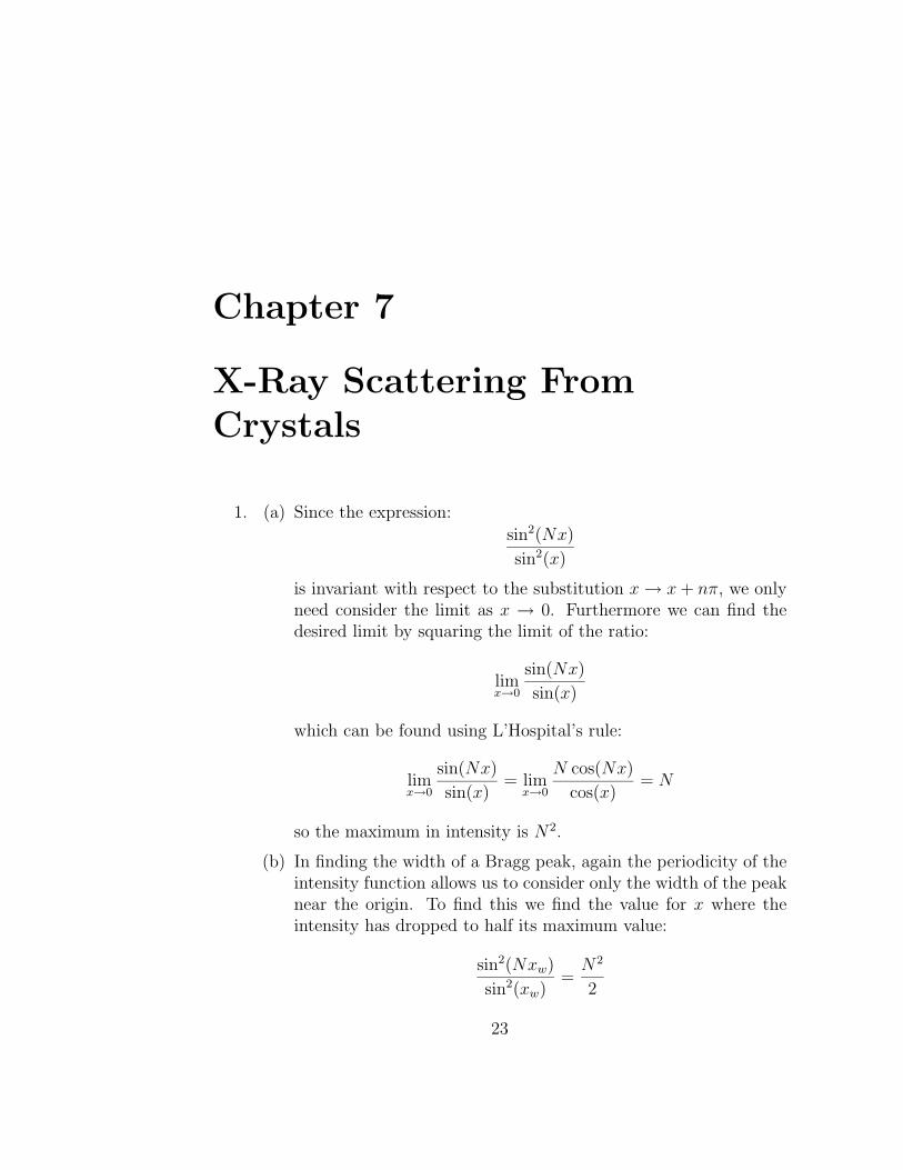
1. (a) Since the expression:

sin2(Nx)

sin2(x)

is invariant with respect to the substitution x→ x+ nπ, we onlyneed consider the limit as x → 0. Furthermore we can find thedesired limit by squaring the limit of the ratio:

limx→0

sin(Nx)

sin(x)

which can be found using L’Hospital’s rule:

limx→0

sin(Nx)

sin(x)= lim

x→0

N cos(Nx)

cos(x)= N

so the maximum in intensity is N2.

(b) In finding the width of a Bragg peak, again the periodicity of theintensity function allows us to consider only the width of the peaknear the origin. To find this we find the value for x where theintensity has dropped to half its maximum value:

sin2(Nxw)

sin2(xw)=N2

2

23

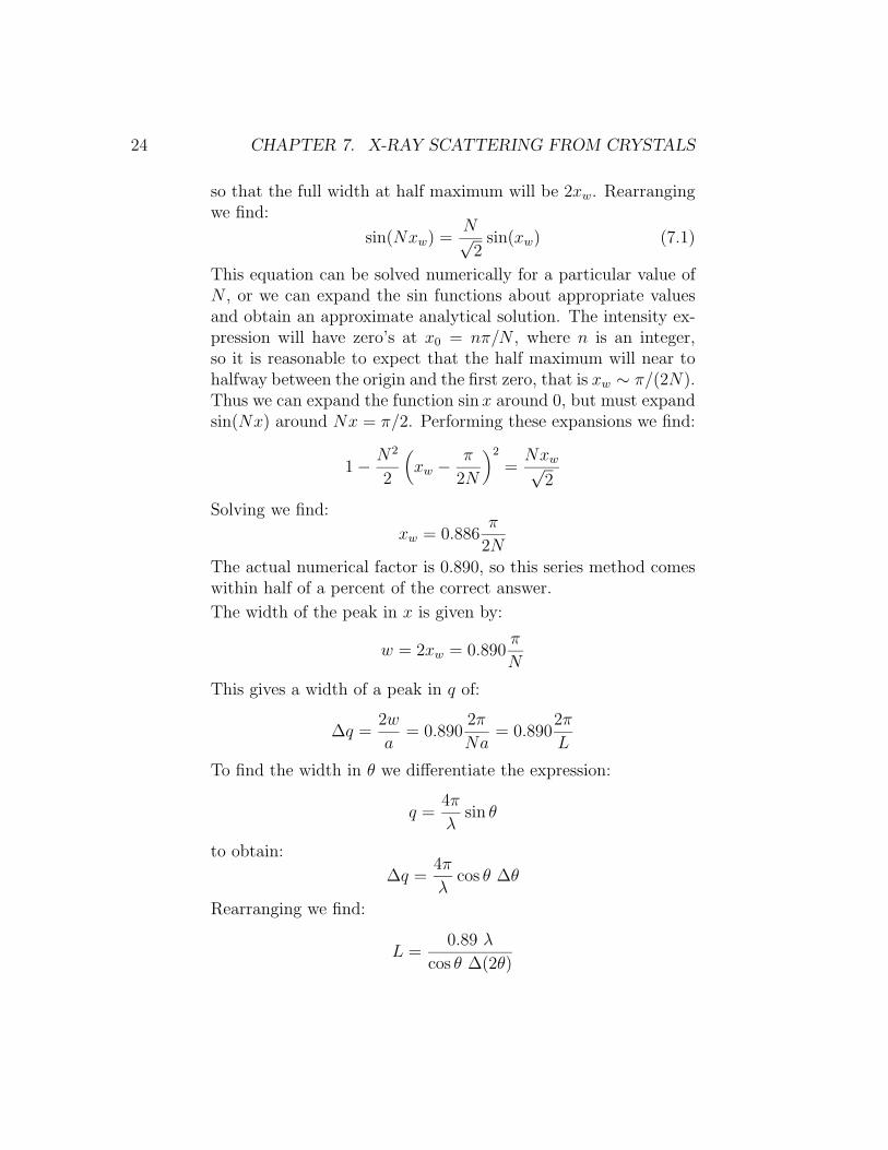
24 CHAPTER 7. X-RAY SCATTERING FROM CRYSTALS

so that the full width at half maximum will be 2xw. Rearrangingwe find:

sin(Nxw) =N√

2sin(xw) (7.1)

This equation can be solved numerically for a particular value ofN , or we can expand the sin functions about appropriate valuesand obtain an approximate analytical solution. The intensity ex-pression will have zero’s at x0 = nπ/N , where n is an integer,so it is reasonable to expect that the half maximum will near tohalfway between the origin and the first zero, that is xw ∼ π/(2N).Thus we can expand the function sin x around 0, but must expandsin(Nx) around Nx = π/2. Performing these expansions we find:

1− N2

2

(xw −

π

2N

)2

=Nxw√

2

Solving we find:

xw = 0.886π

2NThe actual numerical factor is 0.890, so this series method comeswithin half of a percent of the correct answer.

The width of the peak in x is given by:

w = 2xw = 0.890π

N

This gives a width of a peak in q of:

∆q =2w

a= 0.890

2π

Na= 0.890

2π

L

To find the width in θ we differentiate the expression:

q =4π

λsin θ

to obtain:

∆q =4π

λcos θ ∆θ

Rearranging we find:

L =0.89 λ

cos θ ∆(2θ)

25

(c) The subsidiary maximum between the Bragg peaks occur whenthe numerator of the intensity function has maxima. This occursat:

xsm =(n+

1

2

)π

N; n = 1, 2, 3, . . . , N − 1

There are a total of N−2 of these maximum between Bragg peaks.

2. (a) To calculate accurately the thickness of the film using a ruler andFig. 8.11, we need to find a dimension in the figure which can beaccurately measured with a ruler and which correlates with thethickness of the film. We could measure the main peak width andextract from that the thickness of the film as in the problem in thehomework, but it is difficult to measure the width of such a narrowpeak with just a ruler. The many subsidiary maxima provide uswith a better way. These subsidiary maxima are have spacing inq of ∆q = 2π/t, where t is the film thickness. We can measure thewidth in angle for a given number of oscillations and accuratelyextract the average oscillation width in that range by dividing theangular width for many oscillations by the number of oscillations.I found that 32 fringes on the left-hand side of the peak covereda linear distance on the figure of 34.8 mm. I measured also thatthere were about 6.45 mm/degree on this figure, so I find theaverage angular width for the fringes in this region to be ∆(2θ) =0.169 degrees, so that the angular width of a fringe in radians is∆θ = 1.47× 10−3 radians. Differentiating the expression for q wefind:

∆q =4π

λcos θ ∆θ

So we find:

t =2π

∆q=

λ

2 cos θ ∆θ

Which for 2θ ≈ 28.5 gives t ≈ 435A.

(b) For crystals with two different thicknesses we have fringe spacinggiven by:

∆q1 =2π

t1; and ∆q2 =

2π

t2Near the Bragg peak the subsidiary maxima for the two crystalswill add together, but as we move away from the Bragg peak maxi-mum we the differences in spacing will add up until the maximum


for one crystal will be at the position of the minimum for theother. At this point the subsidiary maxima will be washed out.This is exactly the mechanism for washing out of finite thicknessoscillations due to a continuous distribution of thicknesses.

The maxima and minima for the two crystals coincide at Nw oscil-lations away from the Bragg peak the difference in position of themaximum for the two crystals is equal to half the average spacingof the subsidiary maxima, or:

Nw(∆q1 −∆q2) =∆q1 + ∆q2

4

Inserting ∆q1 = 2π/t1 and ∆q2 = 2π/t2, we find:

Nw =∆q1 + ∆q2

2(∆q1 −∆q2)

=1

4

2π/t1 + 2π/t22π/t1 − 2π/t2

=1

4

t2 + t1t2 − t1

=1

2

〈t〉∆t

where 〈t〉 = (t1 + t2)/2 is the average thickness, and ∆t = t2 − t1.So we have that the difference in thickness is given by:

∆t =〈t〉

2Nw

since there are about 50 oscillations observed on either side of thepeak, we have that the difference in thickness is given by:

∆t =435A

100≈ 4A

which is about two lattice planes.

3. (a) For the FCC real space lattice we find:

a2 × a3 =a2

4

∣∣∣∣∣∣∣x y z0 1 11 0 1

∣∣∣∣∣∣∣ =a2

4(x + y − z)

27

so that the cell volume is given by:

Vcell = a1 · a2 × a3 =a3

8(1 + 1) =

a3

4

and the reciprocal lattice vector b1 is given by:

b1 =a2 × a3

a1 · a2 × a3

=1

a(x + y − z)

Similarly we find:

b2 =1

a(−x + y + z)

b3 =1

a(x− y + z)

This is just a BCC lattice with lattice parameter 2/a.

(b) For the BCC real space lattice, we find:

a2 × a3 =a2

4

∣∣∣∣∣∣∣x y z−1 1 11 −1 1

∣∣∣∣∣∣∣ =a2

2(x + y)

so that the cell volume is given by:

Vcell = a1 · a2 × a3 =a3

4(1 + 1) =

a3

2

and the reciprocal lattice vector b1 is given by:

b1 =a2 × a3

a1 · a2 × a3

=(

2

a3

)(a2

2

)(x + y) =

1

a(x + y)

Similarly we find:

b2 =1

a(y + z)

b3 =1

a(x + z)

Which is an FCC lattice with lattice parameter 2/a. Hence thereciprocal lattice of BCC if FCC and vise versa.


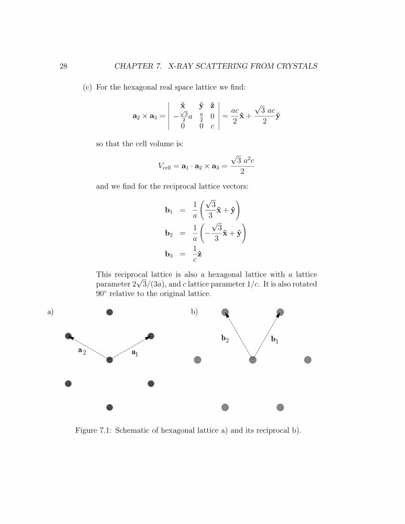
(c) For the hexagonal real space lattice we find:

a2 × a3 =

∣∣∣∣∣∣∣x y z

−√

32a a

20

0 0 c

∣∣∣∣∣∣∣ =ac

2x +

√3 ac

2y

so that the cell volume is:

Vcell = a1 · a2 × a3 =

√3 a2c

2

and we find for the reciprocal lattice vectors:

b1 =1

a

(√3

3x + y

)

b2 =1

a

(−√

3

3x + y

)

b3 =1

cz

This reciprocal lattice is also a hexagonal lattice with a latticeparameter 2

√3/(3a), and c lattice parameter 1/c. It is also rotated

90◦ relative to the original lattice.

a1a2

b1b2

a) b)

Figure 7.1: Schematic of hexagonal lattice a) and its reciprocal b).

29

4. The unit cell of diamond cubic can be taken to be FCC with a basisof (000), and a/4(111), so there will be eight terms in the sum for thestructure factor, corresponding to the atoms at:

(000) a4(111) a

2(110) a

(34

34

14

)a2(101) a

(34

14

34

)a2(011) a

(14

34

34

)We find:

F (q) =∑n

fneiq·rn

= f[1 + eiπ(h+k+l)/2 + eiπ(h+k) + eiπ(3h+3k+l)/2+

eiπ(h+l) + eiπ(3h+k+3l)/2 + eiπ(k+l) + eiπ(h+3k+3l)/2]

=[1 + eiπ(h+k) + eiπ(h+l) + eiπ(k+l)

] [1 + eiπ(h+k+l)/2

]

=

8 h, k, l = even and

h+ k + l = 4× integer4 (1∓ i) h, k, l odd

0 otherwise

In the h, k, l odd case, the minus sign occurs if (h+ k+ l+ 1)/2 is evenand the plus sign if (h+ k + l + 1)/2 is odd.

5. (a) The lattice vectors of the orthorhombic lattice can be taken as:

a1 = ax

a2 = by

a3 = cz

The cell volume is obviously Vcell = abc and the reciprocal latticevectors are:

b1 =1

ax

b2 =1

by

b3 =1

cz


(b) The reciprocal lattice vectors which correspond to the planes (h1, k1, l1)and (h2, k2, l2) are:

Gh1k1l1 =h1

ax +

k1

by +

l1c

z

Gh2k2l2 =h2

ax +

k2

by +

l2c

z

The spacing between sets of (hkl) planes is given by:

dhkl =1

|Ghkl|=

(ha

)2

+

(k

b

)2

+

(l

c

)2−1/2

The angle θ between these two plane normals is found by:

cos θ =Gh1k1l1 ·Gh2k2l2Gh1k1l1Gh2k2l2

= dh1k1l1dh2k2l2

(h1h2

a2+k1k2

b2+l1l2c2

)

6. In general the scattered amplitude from a collection of scatterers isgiven by (in the kinematic approximation):

ε =E0reR

exp [i(ωt− kR)]∑p

fpeiq·Rp

where the sum runs over all the scatterers in the collection. In thiscase, the position vectors can be written as:

Rp =

{pax −(N − 1)/2 ≤ p ≤ (N − 1)/20 |p| > (N − 1)/2

so the sum in the above expression for scattered amplitude becomes:

∑p

fpeiq·Rp =

(N−1)/2∑p=−(N−1)/2

fpeipqxa

We can perform this sum by making the substitution p′ = p+(N−1)/2.This leads to:∑

p

fpeiq·Rp = e−iqxa(N−1)/2

N−1∑p′=0

fpeip′qxa

= f

(e−iqxaN/2

e−iqxa/2

)(1− eiqxaN1− eiqxa

)

= fsin qxaN/2

sin qxa/2

31

where we have pulled f out of the sum since for this problem they areidentical scatterers.

In this problem you are asked to describe the scattered amplitude, soyou must describe the behavior of the scattered amplitude as a functionof the scattering vector q.

(a) In this part the scatterers are point charge electrons. Hence f = 1.The scattered amplitude is independent of the y and z compo-nents of the scattering vector so that the scattered amplitude iseverywhere the same on planes which are perpendicular to the xdirection. The scattered amplitude has a maximum in magnitudeat the condition qxa/2 = nπ, which leads to a condition for themaximum of:

qmaxx =

2πn

awhich is really the Bragg condition for this one-dimensional crys-tal. However, instead of Bragg points, we have Bragg planes ofconstant amplitude perpendicular to the x axis with spacing 2π/a.A scattering vector which terminates on one of these Bragg planessatisfies the condition for a maximum in scattered amplitude.

(b) For the case where we have atoms rather than point electrons, theatomic scattering factor f is no longer a constant independent ofq. Hence the magnitude of the scattered amplitude is no longera constant on one of the Bragg planes, and drops off with thedependence of f(q) away from the x-axis.

7. (a) The scattering factor for this electron distribution is found bytaking the Fourier transform in the normal fashion:

f =∫ρ eiq·r dV

= ρ0

∫ ∞∞

δ(z) eiqzz dz∫ a/2

−a/2eiqxx dx

∫ a/2

−a/2eiqyy dy

= a2ρ0

(sin qxa/2

qxa/2

)(sin qya/2

qya/2

)

(b) For q along the z-axis, the scattering factor becomes

f = a2ρ0


which is just the total number of electrons in each plate. Thediffracted intensity from N of these plates stacked along the z-axis with spacing d is then just

I =I0r

2e

R2(a2ρ0)2

(N−1∑n=0

einqzd)2

= I0

(reaρ0

R

)2 sin2 Nqzd/2

sin2 qZd/2

This, of course, will have peaks at qz = 2Π/d.

8. The general expression for scattered intensity in electron units froma collection of atoms can be found by squaring and normalizing Eqn.8.11:

Ieu =

∣∣∣∣∣∑p

fpeiq·Rp

∣∣∣∣∣2

where the sum runs over all the atoms in the solid. Note that theexponent in the sum involves the dot product of q and the positionvector for the atoms. Hence any change in the position of the atomswhich does not have a component along the direction of q will have noeffect on the observed diffraction. Hence, movement of the atoms in adirection perpendicular to [111] direction will not affect the (111) peak,so the stacking faults as described in this problem have no effect.

9. The scattered intensity is given by our general formula:

I(q) =(E0reR

)|F (q)|2

3∏j=1

sin(Nj

q·aj2

)sin

(q·aj

2

)2

In this case N+1 = N2 = 100 and N3 = 10. We have a simple cubicstructure so F (q) is just the atomic scattering factor f(q). There willbe peaks at

qB = 2πGhkl = 2π

(h

x

a+ k

y

a+ l

z

a

)The peaks will have widths:

∆qx = ∆qy =2π

100a; ∆qz =

2π

10a

A cross section of the x− z plane of this intensity is shown in Fig. 7.2.

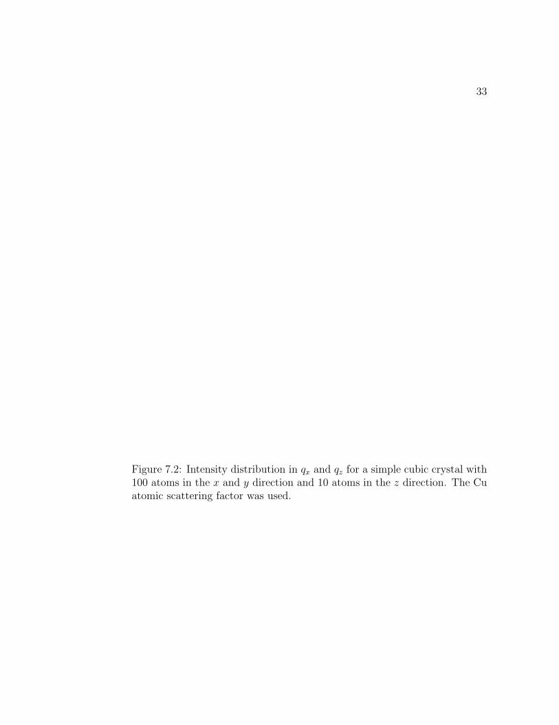
33

Figure 7.2: Intensity distribution in qx and qz for a simple cubic crystal with100 atoms in the x and y direction and 10 atoms in the z direction. The Cuatomic scattering factor was used.


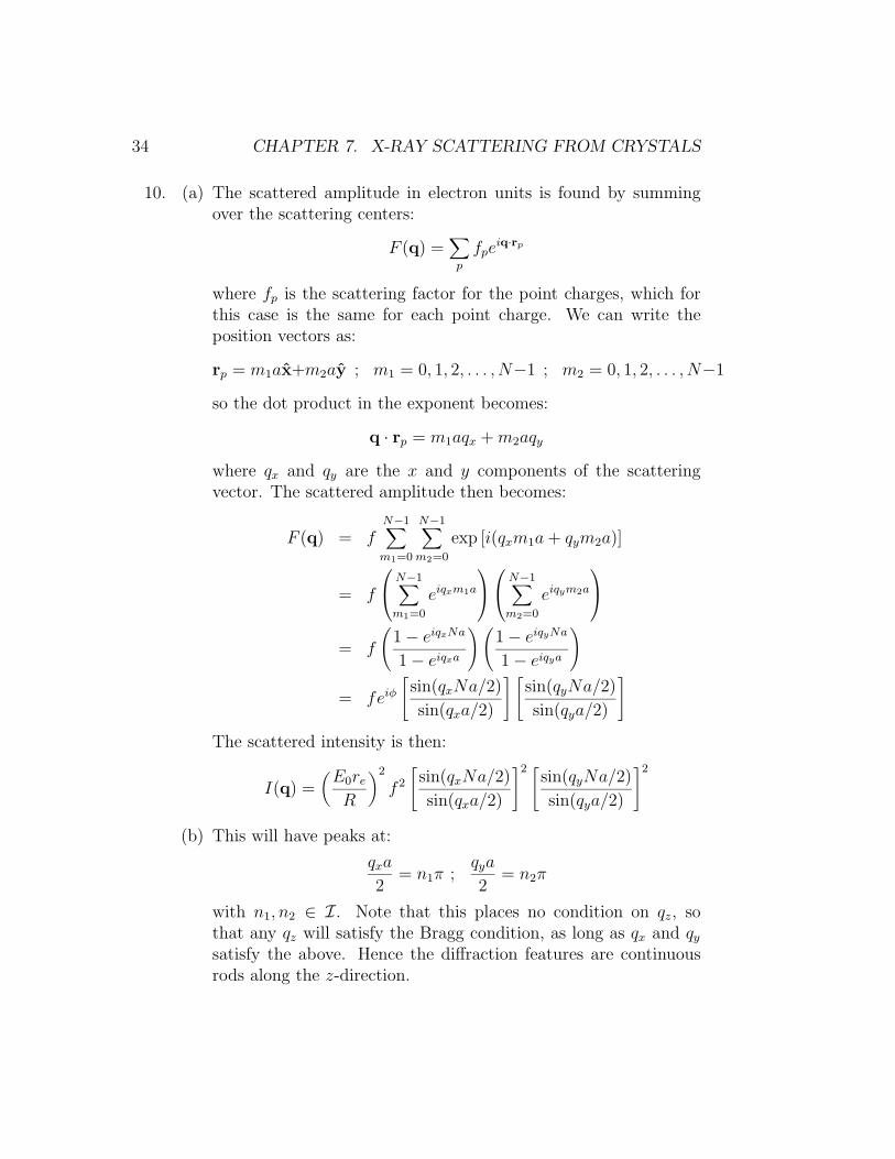
10. (a) The scattered amplitude in electron units is found by summingover the scattering centers:

F (q) =∑p

fpeiq·rp

where fp is the scattering factor for the point charges, which forthis case is the same for each point charge. We can write theposition vectors as:

rp = m1ax+m2ay ; m1 = 0, 1, 2, . . . , N−1 ; m2 = 0, 1, 2, . . . , N−1

so the dot product in the exponent becomes:

q · rp = m1aqx +m2aqy

where qx and qy are the x and y components of the scatteringvector. The scattered amplitude then becomes:

F (q) = fN−1∑m1=0

N−1∑m2=0

exp [i(qxm1a+ qym2a)]

= f

N−1∑m1=0

eiqxm1a

N−1∑m2=0

eiqym2a

= f

(1− eiqxNa1− eiqxa

)(1− eiqyNa1− eiqya

)

= feiφ[

sin(qxNa/2)

sin(qxa/2)

] [sin(qyNa/2)

sin(qya/2)

]

The scattered intensity is then:

I(q) =(E0reR

)2

f 2

[sin(qxNa/2)

sin(qxa/2)

]2 [sin(qyNa/2)

sin(qya/2)

]2

(b) This will have peaks at:

qxa

2= n1π ;

qya

2= n2π

with n1, n2 ∈ I. Note that this places no condition on qz, sothat any qz will satisfy the Bragg condition, as long as qx and qysatisfy the above. Hence the diffraction features are continuousrods along the z-direction.

35

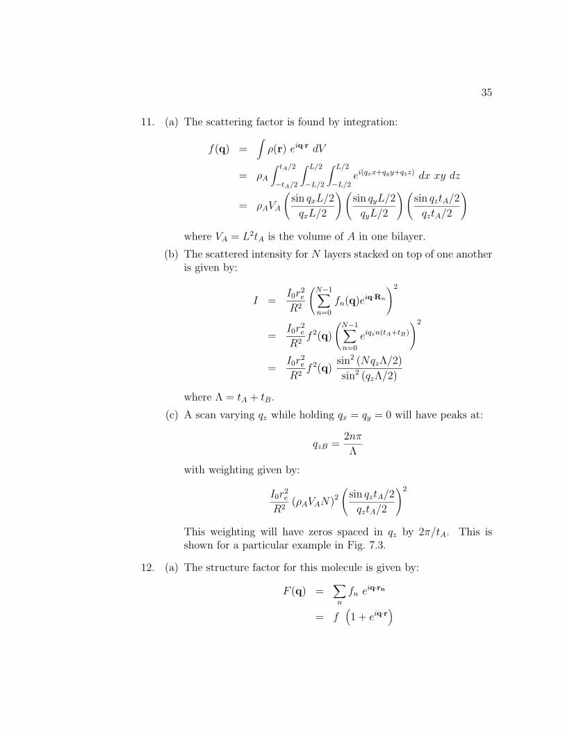
11. (a) The scattering factor is found by integration:

f(q) =∫ρ(r) eiq·r dV

= ρA

∫ tA/2

−tA/2

∫ L/2

−L/2

∫ L/2

−L/2ei(qxx+qyy+qzz) dx xy dz

= ρAVA

(sin qxL/2

qxL/2

)(sin qyL/2

qyL/2

)(sin qztA/2

qztA/2

)

where VA = L2tA is the volume of A in one bilayer.

(b) The scattered intensity for N layers stacked on top of one anotheris given by:

I =I0r

2e

R2

(N−1∑n=0

fn(q)eiq·Rn

)2

=I0r

2e

R2f 2(q)

(N−1∑n=0

eiqzn(tA+tB)

)2

=I0r

2e

R2f 2(q)

sin2 (NqzΛ/2)

sin2 (qzΛ/2)

where Λ = tA + tB.

(c) A scan varying qz while holding qx = qy = 0 will have peaks at:

qzB =2nπ

Λ

with weighting given by:

I0r2e

R2(ρAVAN)2

(sin qztA/2

qztA/2

)2

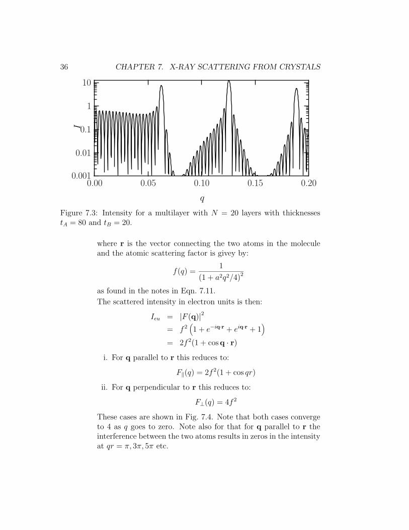
This weighting will have zeros spaced in qz by 2π/tA. This isshown for a particular example in Fig. 7.3.

12. (a) The structure factor for this molecule is given by:

F (q) =∑n

fn eiq·rn

= f(1 + eiq·r

)

0.001

0.01

0.1

1

10I

0.200.150.100.050.00

q


Figure 7.3: Intensity for a multilayer with N = 20 layers with thicknessestA = 80 and tB = 20.

where r is the vector connecting the two atoms in the moleculeand the atomic scattering factor is givey by:

f(q) =1

(1 + a2q2/4)2

as found in the notes in Eqn. 7.11.

The scattered intensity in electron units is then:

Ieu = |F (q)|2

= f 2(1 + e−iq·r + eiq·r + 1

)= 2f 2(1 + cos q · r)

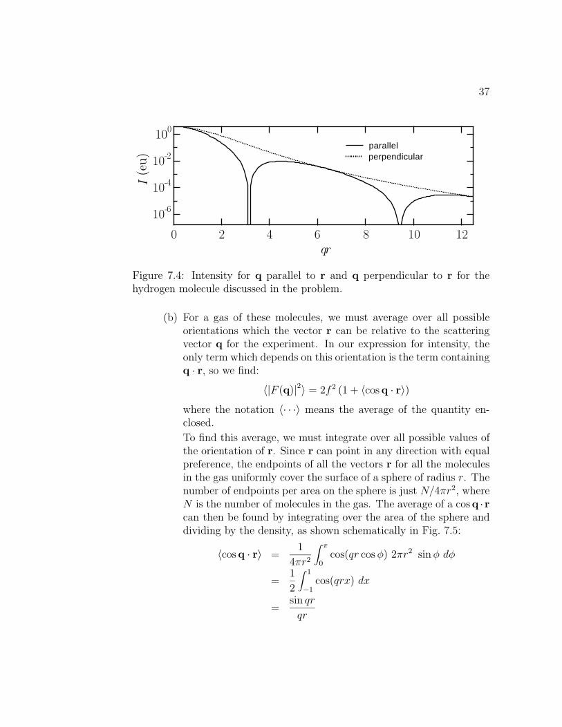
i. For q parallel to r this reduces to:

F‖(q) = 2f2(1 + cos qr)

ii. For q perpendicular to r this reduces to:

F⊥(q) = 4f2

These cases are shown in Fig. 7.4. Note that both cases convergeto 4 as q goes to zero. Note also for that for q parallel to r theinterference between the two atoms results in zeros in the intensityat qr = π, 3π, 5π etc.

10-6

10-4

10-2

100

I (e

u)

121086420qr

parallel perpendicular

37

Figure 7.4: Intensity for q parallel to r and q perpendicular to r for thehydrogen molecule discussed in the problem.

(b) For a gas of these molecules, we must average over all possibleorientations which the vector r can be relative to the scatteringvector q for the experiment. In our expression for intensity, theonly term which depends on this orientation is the term containingq · r, so we find:

〈|F (q)|2〉 = 2f2 (1 + 〈cos q · r〉)where the notation 〈· · ·〉 means the average of the quantity en-closed.

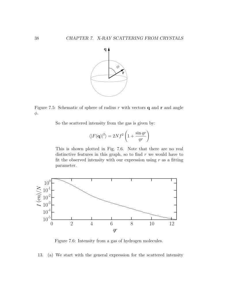
To find this average, we must integrate over all possible values ofthe orientation of r. Since r can point in any direction with equalpreference, the endpoints of all the vectors r for all the moleculesin the gas uniformly cover the surface of a sphere of radius r. Thenumber of endpoints per area on the sphere is just N/4πr2, whereN is the number of molecules in the gas. The average of a cos q ·rcan then be found by integrating over the area of the sphere anddividing by the density, as shown schematically in Fig. 7.5:

〈cos q · r〉 =1

4πr2

∫ π

0cos(qr cosφ) 2πr2 sinφ dφ

=1

2

∫ 1

−1cos(qrx) dx

=sin qr

qr

10-5

10-4

10-3

10-2

10-1

100

I (e

u)/

N

121086420qr


r

q

φ

Figure 7.5: Schematic of sphere of radius r with vectors q and r and angleφ.

So the scattered intensity from the gas is given by:

〈|F (q)|2〉 = 2Nf 2

(1 +

sin qr

qr

)

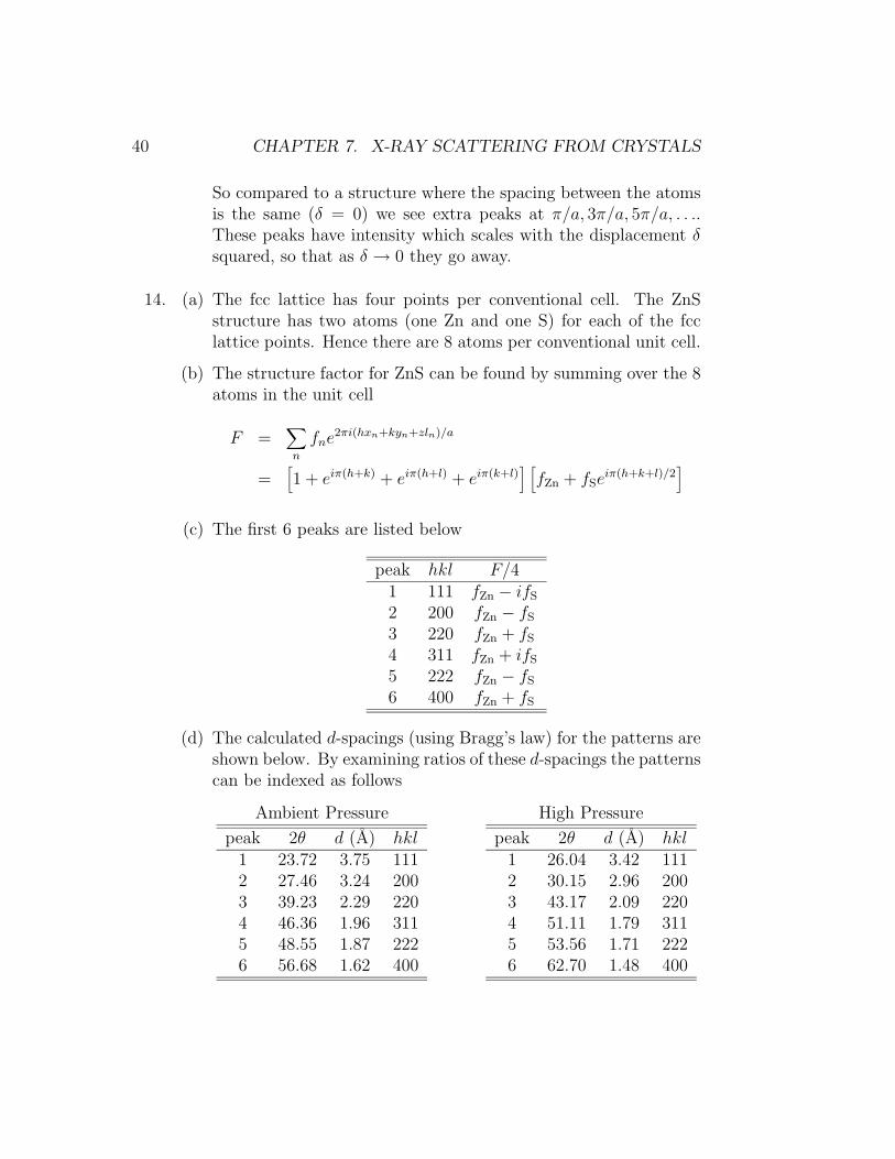
This is shown plotted in Fig. 7.6. Note that there are no realdistinctive features in this graph, so to find r we would have tofit the observed intensity with our expression using r as a fittingparameter.

Figure 7.6: Intensity from a gas of hydrogen molecules.

13. (a) We start with the general expression for the scattered intensity

39

for a collection of atoms

Ieu =

[∑p

fpeiq·rp

]2

For this case the positions of the atoms can be written as a sumof the position of the cell plus the position within the cell:

rp = 2max+ rn

where rn is the position of the atom within the cell and takes thevalues:

r1 = 0 and r2 = (a+ δ)x

for the two atoms within each cell. Hence the intensity becomes:

Ieu = f 2

(N−1∑m=0

eiqx2am

)2 (1 + eiqx(a+δ)

)2

= 2f 2

(sin qxaN

sin qxa

)2

[1 + cos qx(a+ δ)]

where qx is the component of q along the x-direction, and wherewe have used the sum we performed earlier in this class. This is aseries of planes of intensity perpendicular to the x-axis and withspacing π/a.

For small δ we find

Ieu ≈ 2f2

(sin qxaN

sin qxa

)2 [1 + cos qxa− qxδ sin qxa−

(qxδ)2

2cos qxa

]

(b) At the point q = πx/a we find

Ieu = 2f2N2 [1 + cosπ(1 + δ/a)]

≈ f 2N2

(πδ

a

)2

(c) At the point q = 2πx/a we find

Ieu = 2f2N2 [1 + cos 2π(1 + δ/a)]

≈ 4f2N2

1−(πδ

a

)2


So compared to a structure where the spacing between the atomsis the same (δ = 0) we see extra peaks at π/a, 3π/a, 5π/a, . . ..These peaks have intensity which scales with the displacement δsquared, so that as δ → 0 they go away.

14. (a) The fcc lattice has four points per conventional cell. The ZnSstructure has two atoms (one Zn and one S) for each of the fcclattice points. Hence there are 8 atoms per conventional unit cell.

(b) The structure factor for ZnS can be found by summing over the 8atoms in the unit cell

F =∑n

fne2πi(hxn+kyn+zln)/a


] [fZn + fSe

iπ(h+k+l)/2]

(c) The first 6 peaks are listed below

peak hkl F/41 111 fZn − ifS

2 200 fZn − fS

3 220 fZn + fS

4 311 fZn + ifS

5 222 fZn − fS

6 400 fZn + fS

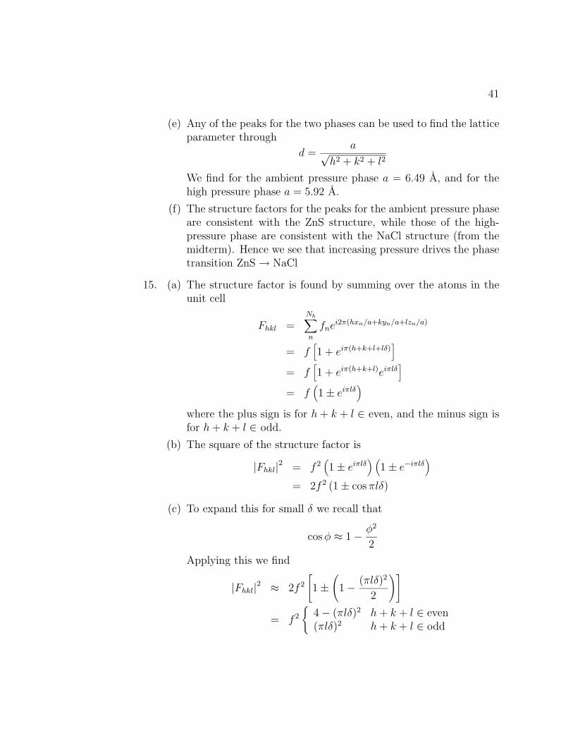
(d) The calculated d-spacings (using Bragg’s law) for the patterns areshown below. By examining ratios of these d-spacings the patternscan be indexed as follows

Ambient Pressure

peak 2θ d (A) hkl1 23.72 3.75 1112 27.46 3.24 2003 39.23 2.29 2204 46.36 1.96 3115 48.55 1.87 2226 56.68 1.62 400

High Pressure

peak 2θ d (A) hkl1 26.04 3.42 1112 30.15 2.96 2003 43.17 2.09 2204 51.11 1.79 3115 53.56 1.71 2226 62.70 1.48 400

41

(e) Any of the peaks for the two phases can be used to find the latticeparameter through

d =a√

h2 + k2 + l2

We find for the ambient pressure phase a = 6.49 A, and for thehigh pressure phase a = 5.92 A.

(f) The structure factors for the peaks for the ambient pressure phaseare consistent with the ZnS structure, while those of the high-pressure phase are consistent with the NaCl structure (from themidterm). Hence we see that increasing pressure drives the phasetransition ZnS→ NaCl

15. (a) The structure factor is found by summing over the atoms in theunit cell

Fhkl =Nb∑n

fnei2π(hxn/a+kyn/a+lzn/a)

= f[1 + eiπ(h+k+l+lδ)

]= f

[1 + eiπ(h+k+l)eiπlδ

]= f

(1± eiπlδ

)where the plus sign is for h+ k + l ∈ even, and the minus sign isfor h+ k + l ∈ odd.

(b) The square of the structure factor is

|Fhkl|2 = f 2(1± eiπlδ

) (1± e−iπlδ

)= 2f 2 (1± cos πlδ)

(c) To expand this for small δ we recall that

cosφ ≈ 1− φ2

2

Applying this we find

|Fhkl|2 ≈ 2f2

[1±

(1− (πlδ)2

2

)]

= f 2

{4− (πlδ)2 h+ k + l ∈ even(πlδ)2 h+ k + l ∈ odd


A change in δ only makes a small relative change in the intensityof the h+k+l ∈ even peaks, while a change in δ makes a relativelylarge change in the intensity of the h+k+l ∈ odd peaks. Hence toexamine changes in δ we will examine the corresponding changesin the h+ k + l ∈ odd peaks.

Chapter 8

Experimental Methods ofDiffraction: Adventures inReciprocal Space

1. (a) The reciprocal lattice vector for the (200) planes is given by:

G200 = 2b1 =2

ax

So when aligned to observe the (200) peak, q is given by:

q = 2πG200 =4π

ax

(b) The path length difference ∆L for the x-rays scattered by planesseparated by a distance a along the direction of q is just:

∆L = 2a sin θ

when on the (200) Bragg peak, the scattering angle satisfies:

λ = 2d sin θ200

where the plane spacing d200 is just given by:

d200 =a

2

43

44 CHAPTER 8. EXPERIMENTAL METHODS OF DIFFRACTION

solving for sin θ200 we find:

sin θ200 =λ

a

which gives:

∆L = 2λ

2. (a) The general reciprocal lattice vector for this cubic lattice is givenby

Ghkl =1

a(hx+ ky + lz)

Therefore, the structure factor for CsCl is

Fhkl = fCs + fCleiπ(h+k+l)

For the (100) peak this becomes

F(100) = fCs − fCl

and for the (200) peak we find

F(200) = fCs + fCl

(b) The structure factor for the chemically disordered BCC lattice is

FBCChkl = 〈f〉

[1 + eiπ(h+k+l)

]As we have seen in class, this gives no peak for the case h+k+ l =odd, while the CsCl structure gives the difference between theatomic scattering factors for this condition. Hence by examiningthe intensity for the k + k + l = odd reflections we can determineif the structure is ordered into the CsCl structure or is chemicallydisordered and so is the BCC structure.

3. The reciprocal lattice vectors for the orthorhombic system are givenby:

b1 =x

a; b2 =

y

b; b3 =

z

c

45

The Bragg condition becomes:

qB = 2πGhkl

= 2π

(hx

a+ky

b+lz

c

)

For the primitive lattice there is only one atom at position r1 = 0 sothe the structure factor is:

F (q) = f(q)

For the base-centered lattice, there are two atoms at positions:

r1 = 0 ; and r2 =ax

2+by

2

so the structure factor becomes:

F (q) = f(q)(1 + eiq·r2

)= f(q)

[1 + eiπ(h+k)

]= f(q)×

{2 h+ k ∈ even0 h+ k ∈ odd

For the body-centered lattice the atom positions are:

r1 = 0 ; and r2 =ax

2+by

2+cz

2


F (q) = f(q)[1 + eiπ(h+k+l)

]= f(q)×

{2 h+ k + l ∈ even0 h+ k + l ∈ odd

For the face-centered lattice, the atom positions are:

r1 = 0 ; r2 =ax

2+by

2; r3 =

ax

2+cz

2; and r4 =

by

2+cz

2


F (q) = f(q)[1 + eiπ(h+k) + eiπ(h+l) + eiπ(k+l)

]= f(q)×

{4 hkl unmixed0 hkl mixed


The structure factors for these structures for the first several peaksare summarized in Table 8.1. One way to distinguish these structureswould be to look for the (100), (001), (110), (101), and (111) peaks.We see from Table 8.1 that the primitive lattice would exhibit all ofthese peaks, the base-centered lattice would exhibit the (001), (110)and (111) peaks, the body-centered lattice would exhibit the (110) and(101) peaks, while the face-centered lattice would exhibit the (111)peak. Hence the structures could be distinguished by looking at theoccurrence of these peaks.

Structure Factorhkl q/2π primitive base body face

100, 010 x/a, y/b f 0 0 0001 z/c f 2f 0 0110 x/a+ y/b f 2f 2f 0

101, 011 x/a+ z/c, y/b+ z/c f 0 2f 0111 x/a+ y/b+ z/c f 2f 0 4f

200, 020, 002 2x/a, 2y/b, 2z/c f 2f 2f 4f

Table 8.1: Structure factor and scattering vector for the first several peaksfor the four orthorhombic lattices.

4. The structure factor F contains the information to distinguish thesetwo phases. In general F is given by:

F (q) =∑n

fneiq·rn

where fn and rn are the atomic scattering factor and the position ofthe nth atom. We are interested in the structure factor Fhkl evaluatedat a Bragg peak where:

q = 2πGhkl = 2π(hb1 + kb2 + lb3)

For the ordered compound, the atoms are at:

Pt atoms a(0, 0, 0), a/2(1, 1, 0)Fe atoms a/2(1, 0, 1), a/2(0, 1, 1)

47

The structure factor F is then:

Fhkl = fPt(1 + eiπ(h+k)

)+ fFe

(eiπ(h+l) + eiπ(k+l)

)=

2 (fPt + fFe) h, k, l unmixed2 (fPt − fFe) h, k even and l odd or h, k odd and l even0 h, k mixed

For the disordered compound, the average atom is on each FCC siteso:

Fhkl =fPt + fFe

2

(1 + eiπ(h+k) + eiπ(h+l) + eiπ(k+l)

)=

{2(fPt + fFe) h, k, l unmixed0 h, k, l mixed

Thus there are some peaks, for example (001), (223), and (112), wherethe ordered phase has a structure factor of 2(fpt − fFe) and the disor-dered phase has a structure factor of 0.

5. (a) The substrate has a cubic structure so the reciprocal lattice vectorsare:

bs1 =1

as0x ; bs2 =

1

as0y ; bs3 =

1

as0z

so that the diffraction vector at the Bragg condition is given by:

qsB = 2πGshkl = 2π(hbs1 + kbs2 + lbs3) =

2π

as0(hx + ky + lz)

The observed substrate peak is at a diffraction vector given by:

qsB = qsx + qsz

Equating components of these two vectors we find:

qs =2πh

as0=

2πl

as0

For the tetragonally distorted film the reciprocal lattice vectorsare given by:

bf1 =1

af‖x ; bf2 =

1

af‖y ; bf3 =

1

af⊥z


and the diffraction vector at the Bragg condition is given by:

qfB = 2πGfhkl = 2π(hbf1 + kbf2 + lbf3) =

2π

af‖(hx + ky) +

2π

af⊥lz

The observed film peak is at a diffraction vector given by:

qfB =qsx

1− δx+

qsz

1− δzEquating the x-components of these vectors we find:

2πh

af‖=

qs

1− δx=

2πh

as0

(1

1− δx

)

Rearranging we find:

af‖ = as0(1− δx)

Similarly, by equating the y-components and rearranging we find:

af⊥ = as0(1− δz)

(b) As we found in this homework set, the width in q of a diffractionpeak is related to the length L of the sample through:

∆q = 0.92π

L

Hence the thickness of the film is:

t ≈ 0.92π

∆qz

and the in-plane grain size is:

lg ≈ 0.92π

∆qx

6. • Sample A

To begin indexing we calculate the d-spacing for each of the peaks.To try to find a pattern, we divide the d-spacing for each peak into

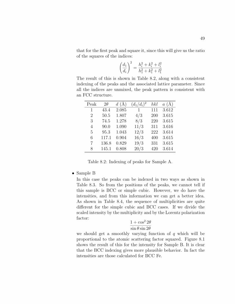
49

that for the first peak and square it, since this will give us the ratioof the squares of the indices:(

d1

di

)2

=h2i + k2

i + l2ih2

1 + k21 + l21

The result of this is shown in Table 8.2, along with a consistentindexing of the peaks and the associated lattice parameter. Sinceall the indices are unmixed, the peak pattern is consistent withan FCC structure.

Peak 2θ d (A) (d1/di)2 hkl a (A)

1 43.4 2.085 1 111 3.6122 50.5 1.807 4/3 200 3.6153 74.5 1.278 8/3 220 3.6154 90.0 1.090 11/3 311 3.6165 95.3 1.043 12/3 222 3.6146 117.1 0.904 16/3 400 3.6157 136.8 0.829 19/3 331 3.6158 145.1 0.808 20/3 420 3.614

Table 8.2: Indexing of peaks for Sample A.

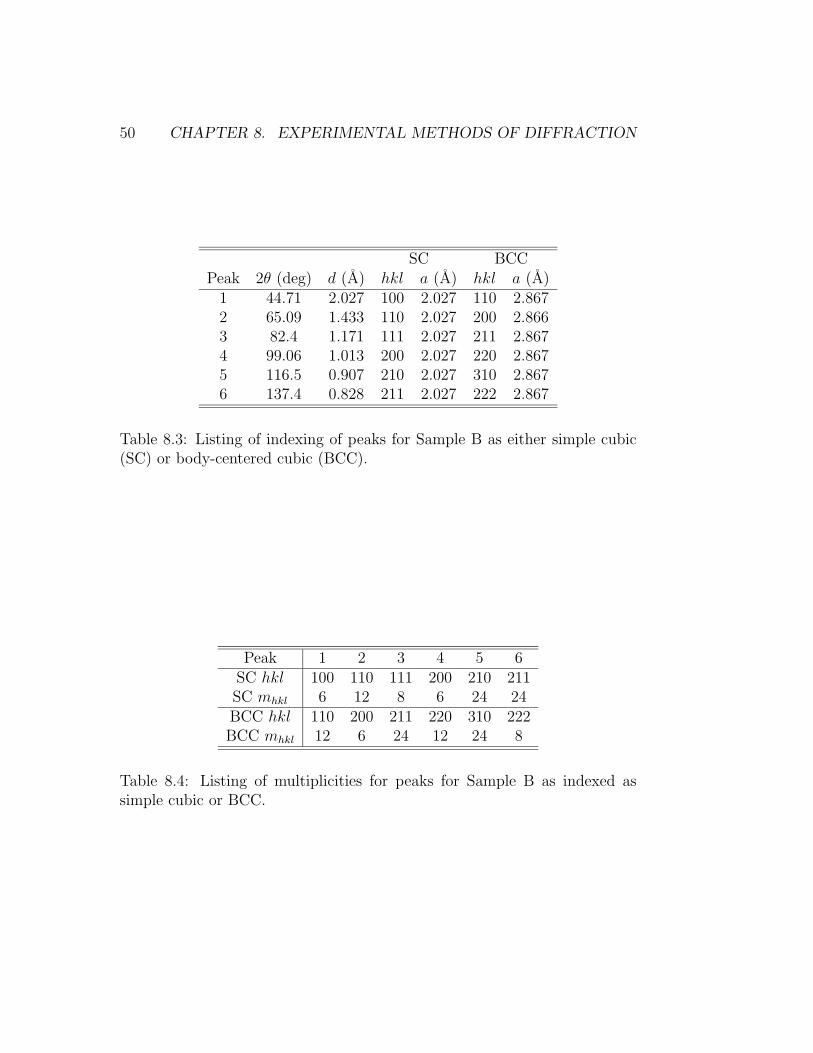
• Sample B

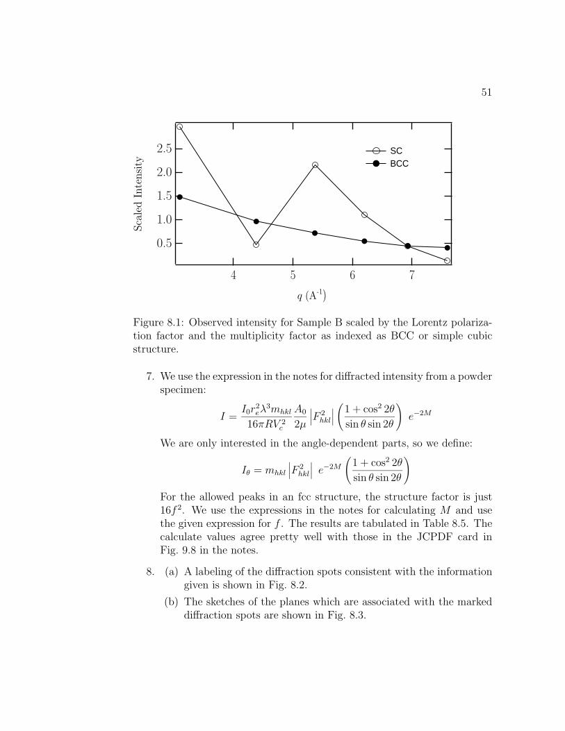
In this case the peaks can be indexed in two ways as shown inTable 8.3. So from the positions of the peaks, we cannot tell ifthis sample is BCC or simple cubic. However, we do have theintensities, and from this information we can get a better idea.As shown in Table 8.4, the sequence of multiplicities are quitedifferent for the simple cubic and BCC cases. If we divide thescaled intensity by the multiplicity and by the Lorentz polarizationfactor:

1 + cos2 2θ

sin θ sin 2θwe should get a smoothly varying function of q which will beproportional to the atomic scattering factor squared. Figure 8.1shows the result of this for the intensity for Sample B. It is clearthat the BCC indexing gives more plausible behavior. In fact theintensities are those calculated for BCC Fe.


SC BCCPeak 2θ (deg) d (A) hkl a (A) hkl a (A)

1 44.71 2.027 100 2.027 110 2.8672 65.09 1.433 110 2.027 200 2.8663 82.4 1.171 111 2.027 211 2.8674 99.06 1.013 200 2.027 220 2.8675 116.5 0.907 210 2.027 310 2.8676 137.4 0.828 211 2.027 222 2.867

Table 8.3: Listing of indexing of peaks for Sample B as either simple cubic(SC) or body-centered cubic (BCC).

Peak 1 2 3 4 5 6SC hkl 100 110 111 200 210 211SC mhkl 6 12 8 6 24 24BCC hkl 110 200 211 220 310 222BCC mhkl 12 6 24 12 24 8

Table 8.4: Listing of multiplicities for peaks for Sample B as indexed assimple cubic or BCC.

51

2.5

2.0

1.5

1.0

0.5

Sca

led I

nte

nsi

ty

7654

q (A-1)

SC BCC

Figure 8.1: Observed intensity for Sample B scaled by the Lorentz polariza-tion factor and the multiplicity factor as indexed as BCC or simple cubicstructure.

7. We use the expression in the notes for diffracted intensity from a powderspecimen:

I =I0r

2eλ

3mhkl

16πRV 2c

A0

2µ

∣∣∣F 2hkl

∣∣∣ (1 + cos2 2θ

sin θ sin 2θ

)e−2M

We are only interested in the angle-dependent parts, so we define:

Iθ = mhkl

∣∣∣F 2hkl

∣∣∣ e−2M

(1 + cos2 2θ

sin θ sin 2θ

)

For the allowed peaks in an fcc structure, the structure factor is just16f 2. We use the expressions in the notes for calculating M and usethe given expression for f . The results are tabulated in Table 8.5. Thecalculate values agree pretty well with those in the JCPDF card inFig. 9.8 in the notes.

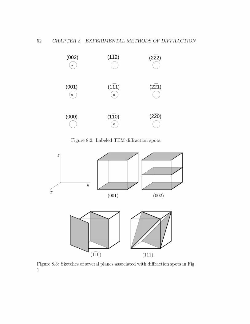
8. (a) A labeling of the diffraction spots consistent with the informationgiven is shown in Fig. 8.2.

(b) The sketches of the planes which are associated with the markeddiffraction spots are shown in Fig. 8.3.


(000)

(001)

*

*

*

*

(002) (112)

(111)

(110)

(222)

(221)

(220)

Figure 8.2: Labeled TEM diffraction spots.

x

y

z

(001) (002)

(110) (111)

Figure 8.3: Sketches of several planes associated with diffraction spots in Fig.1

53

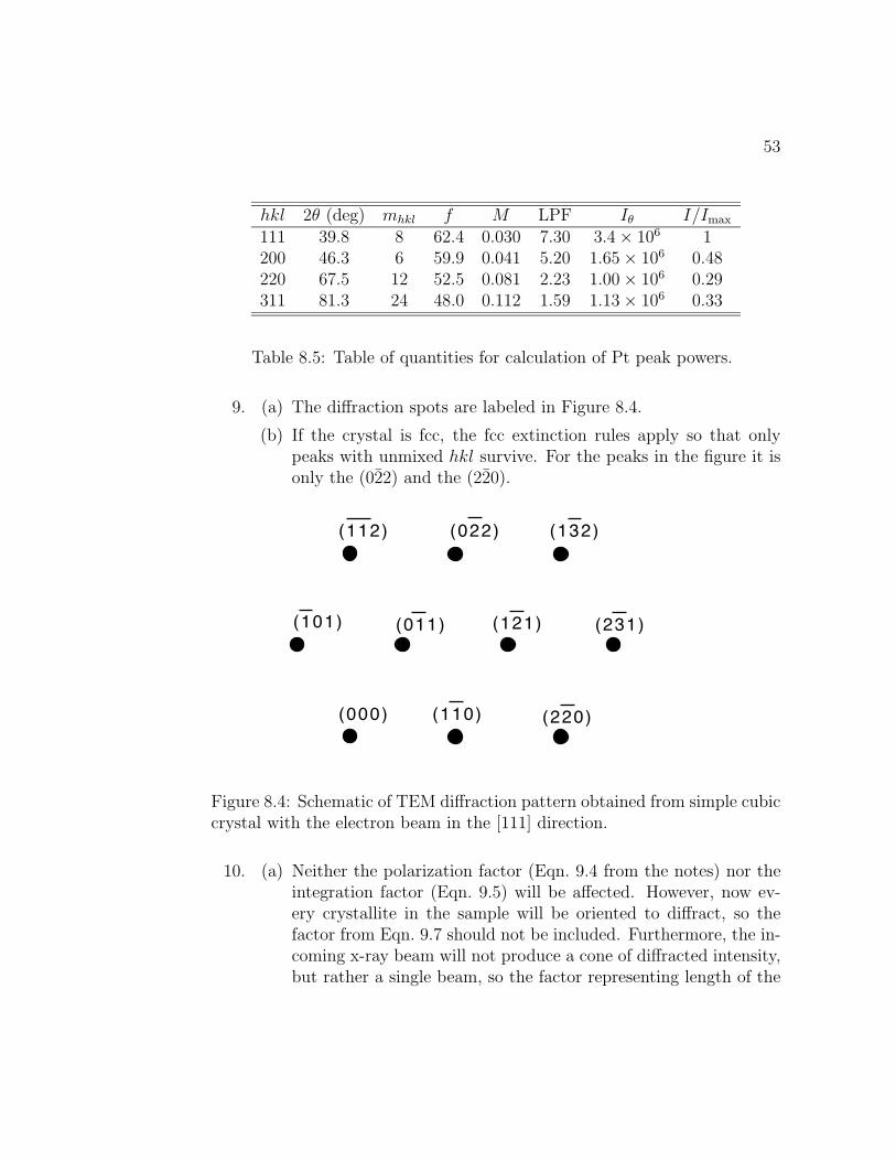
hkl 2θ (deg) mhkl f M LPF Iθ I/Imax

111 39.8 8 62.4 0.030 7.30 3.4× 106 1200 46.3 6 59.9 0.041 5.20 1.65× 106 0.48220 67.5 12 52.5 0.081 2.23 1.00× 106 0.29311 81.3 24 48.0 0.112 1.59 1.13× 106 0.33

Table 8.5: Table of quantities for calculation of Pt peak powers.

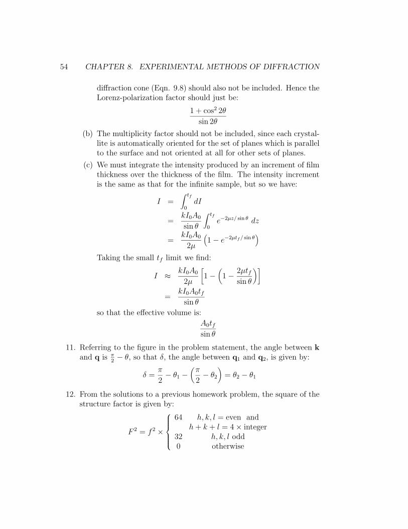
9. (a) The diffraction spots are labeled in Figure 8.4.

(b) If the crystal is fcc, the fcc extinction rules apply so that onlypeaks with unmixed hkl survive. For the peaks in the figure it isonly the (022) and the (220).

(000)

(011)

(110) (220)

(022)

(121) (231)

(132)(112)

(101)

Figure 8.4: Schematic of TEM diffraction pattern obtained from simple cubiccrystal with the electron beam in the [111] direction.

10. (a) Neither the polarization factor (Eqn. 9.4 from the notes) nor theintegration factor (Eqn. 9.5) will be affected. However, now ev-ery crystallite in the sample will be oriented to diffract, so thefactor from Eqn. 9.7 should not be included. Furthermore, the in-coming x-ray beam will not produce a cone of diffracted intensity,but rather a single beam, so the factor representing length of the


diffraction cone (Eqn. 9.8) should also not be included. Hence theLorenz-polarization factor should just be:

1 + cos2 2θ

sin 2θ

(b) The multiplicity factor should not be included, since each crystal-lite is automatically oriented for the set of planes which is parallelto the surface and not oriented at all for other sets of planes.

(c) We must integrate the intensity produced by an increment of filmthickness over the thickness of the film. The intensity incrementis the same as that for the infinite sample, but so we have:

I =∫ tf

0dI

=kI0A0

sin θ

∫ tf

0e−2µz/ sin θ dz

=kI0A0

2µ

(1− e−2µtf/ sin θ

)Taking the small tf limit we find:

I ≈ kI0A0

2µ

[1−

(1− 2µtf

sin θ

)]=

kI0A0tfsin θ

so that the effective volume is:

A0tfsin θ

11. Referring to the figure in the problem statement, the angle between kand q is π

2− θ, so that δ, the angle between q1 and q2, is given by:

δ =π

2− θ1 −

(π

2− θ2

)= θ2 − θ1

12. From the solutions to a previous homework problem, the square of thestructure factor is given by:

F 2 = f 2 ×

64 h, k, l = even and

h+ k + l = 4× integer32 h, k, l odd0 otherwise

55

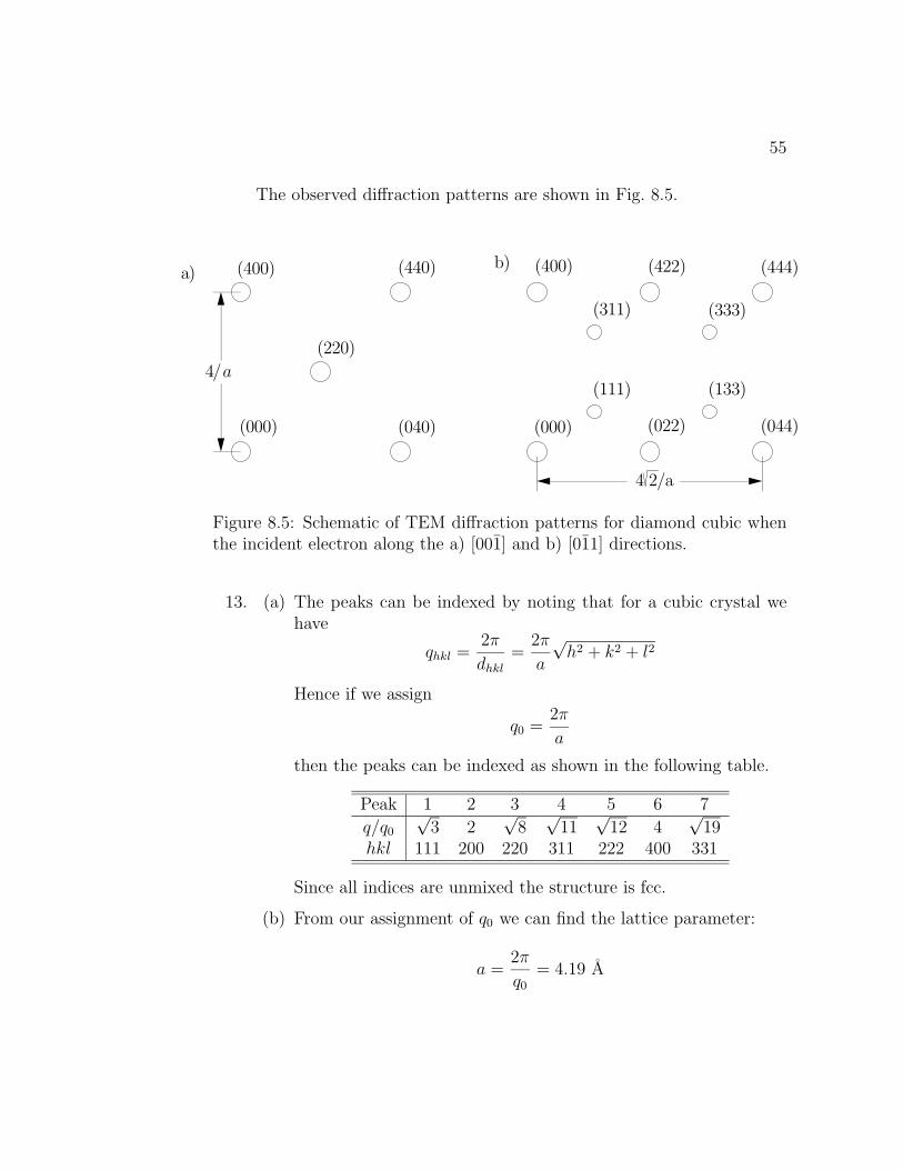
The observed diffraction patterns are shown in Fig. 8.5.

a)

(000)

(400)

(220)

(040)

(440)

4/a

b)

(000)

(400) (422) (444)

(311) (333)

(111) (133)

(022) (044)

4 2/a

Figure 8.5: Schematic of TEM diffraction patterns for diamond cubic whenthe incident electron along the a) [001] and b) [011] directions.

13. (a) The peaks can be indexed by noting that for a cubic crystal wehave

qhkl =2π

dhkl=

2π

a

√h2 + k2 + l2

Hence if we assign

q0 =2π

a

then the peaks can be indexed as shown in the following table.

Peak 1 2 3 4 5 6 7

q/q0

√3 2

√8√

11√

12 4√

19hkl 111 200 220 311 222 400 331

Since all indices are unmixed the structure is fcc.

(b) From our assignment of q0 we can find the lattice parameter:

a =2π

q0

= 4.19 A


14. (a) To index the peaks we first calculate d-spacings, as shown in thetable below. Then the ratio of the square of d-spacings is calcu-lated. It is found that this is consistent with a simple cubic latticewith lattice parameter a = 3.26 Aor a bcc structure with latticeparameter a = 2.305 A. However, in the peak sequence for bcc,there is a peak with indices 321 which appears between the 222and 400 peaks. This peak was not observed for this sample, so itis concluded that the sample is simple cubic.

Peak 2θ d(A) (dn/d1)2 hklsc hklbcc1 27.32 3.26 1 100 1102 39.03 2.31 2 110 2003 48.30 1.88 3 111 2114 56.38 1.63 4 200 2205 63.76 1.46 5 210 3106 70.70 1.33 6 211 2227 83.83 1.15 8 220 400

(b) The density is given by

ρ =n(MCu +MZr)

NAa3

where n is the number of formula units per cell and NA is Avo-gadro’s number. Solving for n we find

n =ρa3NA

MCu +MZr

Plugging in numbers we find that n = 1 so there is one formulaunit per cell.

(c) We know we have a cubic cell with one Cu and one Zr atom ineach cell. Although there are several possibilities for the positionsof the atoms in the cell, we can at least think of the simplest,which is to have one atom at the center of the cell and one at thecorner. This is the CsCl structure which has structure factor

Fhkl = fA + fBeiπ(h+k+l)

Thus for peak 1 which is the (100) peak we have

F100 = fA − fB

57

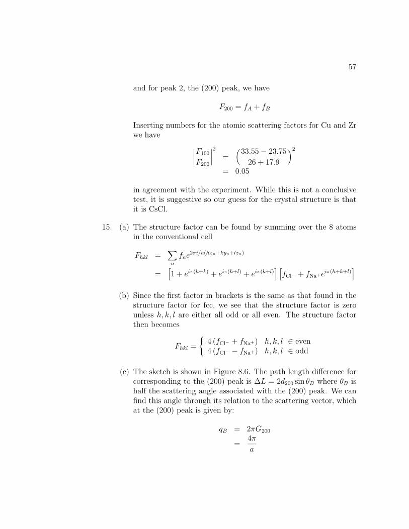
and for peak 2, the (200) peak, we have

F200 = fA + fB

Inserting numbers for the atomic scattering factors for Cu and Zrwe have ∣∣∣∣F100

F200

∣∣∣∣2 =(

33.55− 23.75

26 + 17.9

)2

= 0.05

in agreement with the experiment. While this is not a conclusivetest, it is suggestive so our guess for the crystal structure is thatit is CsCl.

15. (a) The structure factor can be found by summing over the 8 atomsin the conventional cell

Fhkl =∑n

fne2πi/a(hxn+kyn+lzn)


] [fCl− + fNa+eiπ(h+k+l)

](b) Since the first factor in brackets is the same as that found in the

structure factor for fcc, we see that the structure factor is zerounless h, k, l are either all odd or all even. The structure factorthen becomes

Fhkl =

{4 (fCl− + fNa+) h, k, l ∈ even4 (fCl− − fNa+) h, k, l ∈ odd

(c) The sketch is shown in Figure 8.6. The path length difference forcorresponding to the (200) peak is ∆L = 2d200 sin θB where θB ishalf the scattering angle associated with the (200) peak. We canfind this angle through its relation to the scattering vector, whichat the (200) peak is given by:

qB = 2πG200

=4π

a


Hence

sin θB =λ

4πqB

=λ

a

Hence the path difference is

∆L = 2d200 sin θB

= 2(a

2

)(λ

a

)= λ

qk

a

k'

Figure 8.6: Schematic of diffraction condition for the (200) peak in NaClstructure.

(d) For the case of two identical atoms we let fCl− → fNa+ → f andwe find that

Fhkl =

{8 h, k, l ∈ even0 otherwise

This results in a reciprocal lattice which is just simple cubic with areciprocal lattice parameter of 2/a (Figure 8.7). This suggests thatwe could simplify the problem by noticing that the real lattice hasbecome a simple cubic lattice with a new lattice parameter halfthat of the original.

59

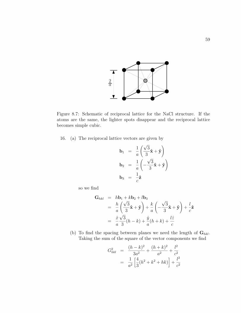
2a

Figure 8.7: Schematic of reciprocal lattice for the NaCl structure. If theatoms are the same, the lighter spots disappear and the reciprocal latticebecomes simple cubic.

16. (a) The reciprocal lattice vectors are given by

b1 =1

a

(√3

3x + y

)

b2 =1

a

(−√

3

3x + y

)

b3 =1

cz

so we find

Ghkl = hb1 + kb2 + lb3

=h

a

(√3

3x + y

)+k

a

(−√

3

3x + y

)+l

cz

=x

a

√3

3(h− k) +

y

a(h+ k) +

lz

c

(b) To find the spacing between planes we need the length of Ghkl.Taking the sum of the square of the vector components we find

G2hkl =

(h− k)2

3a2+

(h+ k)2

a2+l2

c2

=1

a2

[4

3(h2 + k2 + hk)

]+l2

c2


Hence the plane spacing is given by

dhkl =1

Ghkl

=

{[4

3a2(h2 + k2 + hk)

]+l2

c2

}−1/2

(c) If c =√

8/3 a we find:

dhkl = a[4

3(h2 + k2 + hk) +

3

8l2]−1/2

Hence

d002 =√

2/3 a = 0.816 a

d110 = a/2 = 0.5 a

d101 =√

24/41 a = 0.765 a

Since the d-spacing and scattering angle are related through λ =2dhkl sin θ, the largest d will have the smallest scattering angle sothe peaks occur in the order: (002),(101),(110)

Education

Wave diffraction