Tensor Completion for PDEs with uncertain coefficients and Bayesian Update techniques

Tensor completion for PDEs with uncertaincoefficients and Bayesian Update

Alexander Litvinenko(joint work with E. Zander, B. Rosic, O. Pajonk, H. Matthies)

Center for UncertaintyQuantification


Center for Uncertainty Quantification Logo Lock-up

http://sri-uq.kaust.edu.sa/

Extreme Computing Research Center, KAUST

Alexander Litvinenko (joint work with E. Zander, B. Rosic, O. Pajonk, H. Matthies)Tensor completion for PDEs with uncertain coefficients and Bayesian Update

http://sri-uq.kaust.edu.sa/

4*

The structure of the talk

Part I (Stochastic forward problem):1. Motivation2. Elliptic PDE with uncertain coefficients3. Discretization and low-rank tensor approximations

Part II (Bayesian update):1. Bayesian update surrogate2. Examples

Part III (Tensor completion):1. Problem setup2. Tensor completion for Bayesian Update

4*

Motivation to do Uncertainty Quantification (UQ)

Motivation: there is an urgent need to quantify and reduce theuncertainty in output quantities of computer simulations withincomplex (multiscale-multiphysics) applications.

Typical challenges: classical sampling methods are often veryinefficient, whereas straightforward functional representationsare subject to the well-known Curse of Dimensionality.Nowadays computational predictions are used in criticalengineering decisions and thanks to modern computers we areable to simulate very complex phenomena. But, how reliableare these predictions? Can they be trusted?

Example: Saudi Aramco currently has a simulator,GigaPOWERS, which runs with 9 billion cells. How sensitiveare the simulation results with respect to the unknown reservoirproperties?




3 / 30

4*

Part I: Stochastic forward problem

Part I: Stochastic Galerkin method to solveelliptic PDE with uncertain coefficients

4*

PDE with uncertain coefficient and RHS

Consider− div(κ(x , ω)∇u(x , ω)) = f (x , ω) in G × Ω, G ⊂ R2,u = 0 on ∂G, (1)

where κ(x , ω) - uncertain diffusion coefficient. Since κ positive,usually κ(x , ω) = eγ(x ,ω).For well-posedness see [Sarkis 09, Gittelson 10, H.J.Starkloff11, Ullmann 10].Further we will assume that covκ(x , y) is given.




4 / 30

4*

My previous work

After applying the stochastic Galerkin method, obtain:Ku = f, where all ingredients are represented in a tensor format

Compute maxu, var(u), level sets of u, sign(u)[1] Efficient Analysis of High Dimensional Data in Tensor Formats,

Espig, Hackbusch, A.L., Matthies and Zander, 2012.

Research which ingredients influence on the tensor rank of K[2] Efficient low-rank approximation of the stochastic Galerkin matrix in tensor formats,

Wahnert, Espig, Hackbusch, A.L., Matthies, 2013.

Approximate κ(x , ω), stochastic Galerkin operator K in TensorTrain (TT) format, solve for u, postprocessing[3] Polynomial Chaos Expansion of random coefficients and the solution of stochastic

partial differential equations in the Tensor Train format, Dolgov, Litvinenko, Khoromskij, Matthies, 2016.




5 / 30

4*

Canonical and Tucker tensor formats

Definition and Examples of tensors




6 / 30

4*

Canonical and Tucker tensor formats

[Pictures are taken from B. Khoromskij and A. Auer lecture course]

Storage: O(nd )→ O(dRn) and O(Rd + dRn).




7 / 30

4*

Definition of tensor of order d

Tensor of order d is a multidimensional array over a d-tupleindex set I = I1 × · · · × Id ,

A = [ai1...id : iµ ∈ Iµ] ∈ RI , Iµ = 1, ...,nµ, µ = 1, ..,d .

A is an element of the linear space

Vn =d⊗µ=1

Vµ, Vµ = RIµ

equipped with the Euclidean scalar product 〈·, ·〉 : Vn ×Vn → R,defined as

〈A,B〉 :=∑

(i1...id )∈I

ai1...id bi1...id , for A, B ∈ Vn.




8 / 30

4*

Discretization of elliptic PDE

Now let us discretize our diffusion equation withuncertain coefficients




9 / 30

4*

Karhunen Loeve and Polynomial Chaos Expansions

Apply bothKarhunen Loeve Expansion (KLE):κ(x , ω) = κ0(x) +

∑∞j=1 κjgj(x)ξj(θ(ω)), where

θ = θ(ω) = (θ1(ω), θ2(ω), ..., ),ξj(θ) = 1

κj

∫G (κ(x , ω)− κ0(x)) gj(x)dx .

Polynomial Chaos Expansion (PCE)κ(x , ω) =

∑α κ

(α)(x)Hα(θ), compute ξj(θ) =∑

α∈J ξ(α)j Hα(θ),

where ξ(α)j = 1κj

∫G κ

(α)(x)gj(x)dx .

Further compute ξ(α)j ≈∑s

`=1(ξ`)j∏∞

k=1(ξ`, k )αk .




10 / 30

4*

Final discretized stochastic PDE

Ku = f, where

K:=∑s

`=1K` ⊗⊗M

µ=1∆`µ, K` ∈ RN×N , ∆`µ ∈ RRµ×Rµ ,u:=

∑rj=1 uj ⊗

⊗Mµ=1 ujµ, uj ∈ RN , ujµ ∈ RRµ ,

f:=∑R

k=1 f k ⊗⊗M

µ=1 gkµ, f k ∈ RN and gkµ ∈ RRµ .(Wahnert, Espig, Hackbusch, Litvinenko, Matthies, 2011)

Examples of stochastic Galerkin matrices:




11 / 30

4*

Part II

Part II: Bayesian update

We will speak about Gauss-Markov-Kalman filter for theBayesian updating of parameters in comput. model.

4*

Mathematical setup

Consider

K (u; q) = f ⇒ u = S(f ; q),

where S is solution operator.Operator depends on parameters q ∈ Q,hence state u ∈ U is also function of q:

Measurement operator Y with values in Y:

y = Y (q; u) = Y (q,S(f ; q)).

Examples of measurements:y(ω) =

∫D0

u(ω, x)dx , or u in few points




12 / 30

4*

Random QoI

With state u a RV, the quantity to be measured

y(ω) = Y (q(ω),u(ω)))

is also uncertain, a random variable.Noisy data: y + ε(ω),

where y is the “true” value and a random error ε.

Forecast of the measurement: z(ω) = y(ω) + ε(ω).




13 / 30

4*

Conditional probability and expectation

Classically, Bayes’s theorem gives conditional probability

P(Iq|Mz) =P(Mz |Iq)

P(Mz)P(Iq) (orπq(q|z) =

p(z|q)

Zspq(q));

Expectation with this posterior measure is conditionalexpectation.

Kolmogorov starts from conditional expectation E (·|Mz),from this conditional probability via P(Iq|Mz) = E

(χIq |Mz

).




14 / 30

4*

Conditional expectation

The conditional expectation is defined asorthogonal projection onto the closed subspace L2(Ω,P, σ(z)):

E(q|σ(z)) := PQ∞q = argminq∈L2(Ω,P,σ(z)) ‖q − q‖2L2

The subspace Q∞ := L2(Ω,P, σ(z)) represents the availableinformation.

The update, also called the assimilated valueqa(ω) := PQ∞q = E(q|σ(z)), is a Q-valued RV

and represents new state of knowledge after the measurement.Doob-Dynkin: Q∞ = ϕ ∈ Q : ϕ = φ z, φmeasurable.




15 / 30

4*

Numerical computation of NLBU

Look for ϕ such that q(ξ) = ϕ(z(ξ)), z(ξ) = y(ξ) + ε(ω):

ϕ ≈ ϕ =∑α∈Jp

ϕαΦα(z(ξ))

and minimize ‖q(ξ)− ϕ(z(ξ))‖2L2, where Φα are polynomials

(e.g. Hermite, Laguerre, Chebyshev or something else).Taking derivatives with respect to ϕα:

∂

∂ϕα〈q(ξ)− ϕ(z(ξ)),q(ξ)− ϕ(z(ξ))〉 = 0 ∀α ∈ Jp

Inserting representation for ϕ, obtain:




16 / 30

4*


∂

∂ϕαE

q2(ξ)− 2∑β∈J

qϕβΦβ(z) +∑β,γ∈J

ϕβϕγΦβ(z)Φγ(z)

= 2E

−qΦα(z) +∑β∈J

ϕβΦβ(z)Φα(z)

= 2

∑β∈J

E [Φβ(z)Φα(z)]ϕβ − E [qΦα(z)]

= 0 ∀α ∈ J .




17 / 30

4*


Now, rewriting the last sum in a matrix form, obtain the linearsystem of equations (=: A) to compute coefficients ϕβ: ... ... ...

... E [Φα(z(ξ))Φβ(z(ξ))]...

... ... ...

...ϕβ

...

=

...

E [q(ξ)Φα(z(ξ))]...

,

where α, β ∈ J , A is of size |J | × |J |.




18 / 30

4*


We can rewrite the system above in the compact form:

[Φ] [diag(...wi ...)] [Φ]T

...ϕβ...

= [Φ]

w0q(ξ0)...

wNq(ξN)

[Φ] ∈ RJα×N , [diag(...wi ...)] ∈ RN×N , [Φ] ∈ RJα×N .Solving this system, obtain vector of coefficients (...ϕβ...)

T forall β.Finally, the assimilated parameter qa will be

qa = qf + ϕ(y)− ϕ(z), (2)

z(ξ) = y(ξ) + ε(ω), ϕ =∑

β∈JpϕβΦβ(z(ξ))




19 / 30

4*

Explanation of ” Bayesian Update surrogate” from E. Zander

I Let the stochastic model of the measurement is given by

y =M(q) + ε, ε -measurement noise (3)

I Best estimator ϕ for q given z, i.e.

ϕ = argminϕ E[‖q(·)− ϕ(z(·))‖22]. (4)

I The best estimate (or predictor) of q given themeasurement model is

qM(ξ) = ϕ(z(ξ))). (5)

I The remainder, i.e. the difference between q and qM, isgiven by

q⊥M(ξ) = q(ξ)− qM(ξ), (6)

I Due to the minimisation property of the MMSEestimator—orthogonal to qM(ξ), i.e. cov(q⊥M,qM) = 0.




20 / 30

I In other words,

q(ξ) = qM(ξ) + q⊥M(ξ) (7)

yields an orthogonal decomposition of q.I Actual measurement y , prediction q = ϕ(y). Part qM of q

can be “collapsed” to q. Updated stochastic model q′ isthus given by

q′(ξ) = q + q⊥M(ξ) (8)

q′(ξ) = q(ξ) + (ϕ(y)− ϕ(z(ξ))). (9)




21 / 30

4*

Example: 1D elliptic PDE with uncertain coeffs

−∇ · (κ(x , ξ)∇u(x , ξ)) = f (x , ξ), x ∈ [0,1]

+ Dirichlet random b.c. g(0, ξ) and g(1, ξ).3 measurements: u(0.3) = 22, s.d. 0.2, x(0.5) = 28, s.d. 0.3,x(0.8) = 18, s.d. 0.3.

I κ(x, ξ): N = 100 dofs, M = 5, number of KLE terms 35, beta distribution for κ, Gaussian covκ, cov.length 0.1, multi-variate Hermite polynomial of order pκ = 2;

I RHS f (x, ξ): Mf = 5, number of KLE terms 40, beta distribution for κ, exponential covf , cov. length 0.03,multi-variate Hermite polynomial of order pf = 2;

I b.c. g(x, ξ): Mg = 2, number of KLE terms 2, normal distribution for g, Gaussian covg , cov. length 10,multi-variate Hermite polynomial of order pg = 1;

I pφ = 3 and pu = 3




22 / 30

4*

Example: updating of the solution u

0 0.5 1-20

0

20

40

60

0 0.5 1-20

0

20

40

60

Figure: Original and updated solutions, mean value plus/minus 1,2,3standard deviations

[graphics are built in the stochastic Galerkin library sglib, written by E. Zander in TU Braunschweig]




23 / 30

4*

Example: Updating of the parameter

0 0.5 10

0.5

1

1.5

0 0.5 10

0.5

1

1.5

Figure: Original and updated parameter κ.




24 / 30

4*

Part III. Tensor completion

Now, we consider how toapply Tensor Completion Techniques

for Bayesian Update

In Bayesian Update surrogate, the assimilated PCE coeffs ofparameter qa will beNEW gPCE coeffs=OLD gPCE coeffs + gPCE of UpdateALL INGREDIENTS ARE TENSORS!

qa = qf + ϕ(y)− ϕ(z), (10)

z(ξ) = y(ξ) + ε(ω), qa ∈ RN×#Ja , N = 1..107, #Ja > 1000,#Jf < #Ja.

4*

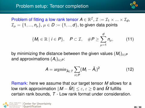
Problem setup: Tensor completion

Problem of fitting a low rank tensor A ∈ RI , I := I1 × ...× Id ,Iµ = 1, ...,nµ, µ ∈ D := 1, ..,d, to given data points

Mi ∈ R | i ∈ P, P ⊂ I, #P ≥d∑µ=1

nµ, (11)

by minimizing the distance between the given values (Mi)i∈Pand approximations (Ai)i∈P :

A = argminA∈T

∑i∈P

(Mi − Ai)2 (12)

Remark: here we assume that our target tensor M allows for alow rank approximation ‖M − M‖ ≤ ε, ε ≥ 0 and M fulfillscertain rank bounds, T - Low rank format under consideration.




26 / 30

4*

Problem setup: Tensor completion

L. Grasedyck et all, 2016, hierarchical and tensor train formatsW. Austin, T, Kolda, D, Kressner, M. Steinlechner et al, CPformat

Goal: Reconstruct tensor with O(log N) number of samples.Methods:1. ALS inspired by LMaFit method for matrix completion,complexity O(r4d#P).2. Alternating directions fitting (ADF), complexity O(r2d#P).




27 / 30

4*

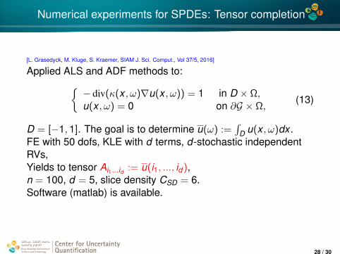
Numerical experiments for SPDEs: Tensor completion

[L. Grasedyck, M. Kluge, S. Kraemer, SIAM J. Sci. Comput., Vol 37/5, 2016]

Applied ALS and ADF methods to:− div(κ(x , ω)∇u(x , ω)) = 1 in D × Ω,u(x , ω) = 0 on ∂G × Ω,

(13)

D = [−1,1]. The goal is to determine u(ω) :=∫

D u(x , ω)dx .FE with 50 dofs, KLE with d terms, d-stochastic independentRVs,Yields to tensor Ai1...id := u(i1, ..., id ),n = 100, d = 5, slice density CSD = 6.Software (matlab) is available.




28 / 30

4*

Example: updating of the solution u

0 0.5 1-20

0

20

40

60

0 0.5 1-20

0

20

40

60

0 0.5 1-20

0

20

40

60

0 0.5 1-20

0

20

40

60

0 0.5 1-20

0

20

40

60

Figure: Original and updated solutions, mean value plus/minus 1,2,3standard deviations. Number of available measurements 0,1,2,3,5

[graphics are built in the stochastic Galerkin library sglib, written by E. Zander in TU Braunschweig]




29 / 30

4*

Conclusion

I Introduced low-rank tensor methods to solve elliptic PDEswith uncertain coefficients,

I Explained how to compute the maximum and the mean inlow-rank tensor format,

I Derived Bayesian update surrogate ϕ (as a linear,quadratic, cubic etc approximation), i.e. computeconditional expectation of q, given measurement y .

I Apply Tensor Completion method to sparse measurementtensor in the likelihood.




30 / 30

Education

Tensor Completion for PDEs with uncertain coefficients and Bayesian Update techniques