Statistics for Social Scienceand Public Policy

Advisors:S.E. Fienberg D. Lievesley 1. Rolph

Springer-Verlag Berlin Heidelberg GmbH

Statistics for Social Science and Public Policy

Brennan: Generalizability Theory.

Devlin/Fienberg/Resnick/Raeder (Eds.) : Intelligence, Genes,and Success: Scientists

Respond to TheBell Curve.

Finkelstein/Ievin: Statistics for Lawyers, SecondEdition.

Gastwirth (Ed.) : Statistical Sciencein the Courtroom.

HandcockiMorris: Relative Distribution Methods in the SocialSciences.

JohnsoniAlbert: OrdinalData Modeling.

Morton/Rolph: PublicPolicyand Statistics: CaseStudiesfromRAND.

Zeisel/Kaye: ProveIt withFigures: Empirical Methods in Law and Litigation.

Robert L. Brennan

Generalizability Theory

Springer

Robert L. BrennanIowa Testing ProgramsUniversity of IowaIowa City, IA 52242-1529USA

Advisors:

Stephen E . FienbergDepartment of StatisticsCarnegie Mellon UniversityPittsburgh, PA 15213USA

lohn RolphDepartment of Information and

Operations ManagementGraduate School of BusinessUniversity of Southern CaliforniaLos Angeles, CA 90089USA

Denise LievesleyInstitute for StatisticsRoom H.113UNESCO7 Place de Fontenoy75352 Paris 07 SPFrance

Library of Congress Cataloging-in-Publication DataBrennan, Robert L.

Generalizability theory / Robert L. Brennanp. cm. - (Statistics for social science and public policy)

Includes bibliographieal references (p. ) and indexes .

I . Psychometries. 2. Psychology-Statistical methods . 3. Analysis ofvariance . 1. Title . H. Series .BF39.B755 2001150' .1 '5 I95-dc2 I 2001032009

Printed on acid- free paper.© 2001 Springer-Verlag Berlin Heidelberg

Originally published by Springer-Verlag Berlin Heidelberg New York in 200I.

Softcover reprint of the hardcover Ist edition 200I

All rights reserved. This work may not be translated or copied in whole or in part without thewritten permission of the publisher

analysis. Use in connection with any form of information storage and retrieval, electronicadaptation, computer software, or by similar or dissimilar methodology now known or hereafterdeveloped is forbidden .The use of general descriptive names, trade names, trademarks, etc ., in this publication, evenif the former are not especially identified, is not to be taken as a sign that such names , asunderstood by the Trade Marks and Merchandise Marks Act, may accordingly be used freely byanyone .

Production managed by Allan Abrams; manufacturing supervised by Jeffrey Taub.Photocomposed copy prepared by the author using It<TEX.

987 654 3 2 I

ISBN 978-1-4419-2938-9 ISBN 978-1-4757-3456-0 (eBook)DOI 10.1007/978-1-4757-3456-0

Springer-Verlag New York Berlin HeidelbergA member 0/ BertelsmannSpringer Science+Business Media GmbH

(Springer-Verlag Berlin Heidelberg GmbH), except for brief excerpts in connection with reviews or scholarly

To Cicely

Preface

In 1972 a monograph by Cronbach, Gleser, Nanda, and Rajaratn am waspublished ent itled The Dependability of Behavioral Measurem ents. Thatbook incorp orat ed, systematized, and extended their previous research intowhat came to be called generalizability theory, which liberalizes classicaltest t heory, in part through the app lication of analysis of variance proce­dures that focus on variance components. Generalizability theory is perhapsth e most broadly defined measurement model currently in existence, andthe Cronbach et al. (1972) t reat ment of the theory represents a major con­tribution to psychometrics. However , as Cronb ach et al. (1972, p. 3) state,t heir book is "complexly organized and by no means simple to follow" and,of course, it is nearly 30 years old.

In 1983, ACT , Inc. pub lished my monograph ent it led Elements of Gen­eralizability Theory, with a slight ly revised version appearing in 1992. Thatt reatment is considerably less comprehensive th an Cronbach et al. (1972)but still det ailed enough to convey much of the richness of the theory andto facilit ate its application. However , t he 1983/1 992 monograph is essen­t ially two decades old, it does not cover mult ivariate generalizability theoryin dept h, and it does not incorporate recent developments in statistics thatbear upon the est imation of variance components. Also, of course, t herehave been numerous developments in genera lizability th eory in the last 20years.

This book provides a much more comprehensive and up-to-date treat ­ment of generalizability th eory. It covers all of t he major topics th at havebeen discusscd in generalizability theory, as weIl as some new ones. In ad-

viii Preface

dition, it provides a synthesis of those parts of the statistiealliterature thatare directly applicable to generalizability theory.

The principal intended audience is measurement practitioners and upper­level graduate students in the behavioral and social sciences, particularlyeducation and psychology. Generalizability theory has broader applicabil­ity, however. Indeed, it might be used in virtually any field that attendsto measurements and their errors. Readers will benefit from some familiar­ity with classieal test theory and analysis of variance, but the treatmentof most topics does not presume specific background. In particular, vari­ance components are a central focus of generalizability theory, but it isnot assumed that readers are familiar with them or with procedures forestimating them.

Although the statistieal aspects of generalizability theory are undeni­ably important, perhaps the most distinguishing feature of the theory is itsconceptual framework, whieh permits a multifaceted perspective on mea­surement error and its components. What makes generalizability theoryboth challenging and useful is that it marries this rieh conceptual frame­work with powerful, but sometimes complicated, statistieal procedures.This book gives substantial attention to both aspects of generalizabilitytheory-the conceptual framework and the statistieal machinery. However,the book per se is neither a treatise on the philosophy of measurement, nora textbook on statistieal procedures. Rather, it integrates those parts ofboth topics that bear upon generalizability theory.

Precursors to generalizability theory are evident in papers written aslong aga as the 1930s. However, generalizability theory per se is relativelynew, it is evolving, and there are a few somewhat different perspectiveson the theory. Most of these perspectives are complementary, or might beviewed as special cases or extensions . Even so, Ijudged it necessary to adoptone principal perspective and maintain it throughout this book. That per­spective is closely aligned with Cronbach et al. (1972), but there are someoccasional differences. For example, except for the last chapter, this bookdoes not emphasize regressed score estimates of universe scores nearly asmuch as Cronbach et al. (1972). Also, there are some notational differences,especially in those chapters that treat multivariate generalizability theory.

There are three sets of chapters in this book. They are ordered in termsof increasing complexity. The fundamentals of univariate generalizabilitytheory are contained in Chapters 1 to 4. They might be used as part of agraduate--levelcourse in advanced measurement. Additional, more challeng­ing topies in univariate theory are covered in Chapters 5 to 8, and Chapters9 to 12 provide my own perspective on multivariate generalizability theory.

The treatment of multivariate generalizability theory is inspired by thework of Cronbach et al. (1972), but there are notieeable differences in em­phasis , coverage, and notational conventions. I have tried to provide thereader with different ways of thinking about multivariate generalizabilitytheory, and I have tried to illustrate its similarities to and differences from

Preface IX

univariate theory. An important goal of this book is to make multivar iategeneralizability theory more accessible to practitioners.

More consideration is given to reliability-like coefficients than is necessi­tated by the theory. However, in my experience, many students and mea­surement practitioners have great difficulty, at least initially, in appreciat­ing the applicability and usefulness of generalizability theory unless theycan relate some of its results to classical reliability coefficients. For thisreason , such coefficients are act ively considered, although the magnitudesof variance components , and particularly error variances, are clearly moreimportant .

Many of the topi cs covered here could be treated using matri x opera tors .With th e except ion of one appendix, however , matrix opera tors are notemployed, because doing so would render the content inaccessible to manystudents and practitioners who might benefit from the theory.

I am grateful to ACT, Inc., for permitting me to use parts of Brennan(1992a). That monograph clearly infiuenced my treatment of Chapters 2to 5 and several appendices. Also, Chapter 1 is largely a revised version ofBrennan (1992b) used with the permission of the publisher , the NationalCouncil on Measurement in Education, and parts of Section 5.4 are fromBrennan (1998) used with permission of the publisher, Sage. I am alsograteful to ACT , Inc. for permitting me access to ACT Assessment dataused for various multivariate examples in the later chapters of this book,to Suzanne Lane for permit ting me to use the QUASAR data referenced inSection 5.4, to Clare Kreiter for the opportunity to analyze data discussedin Section 8.3, and to J udy Ru at Iowa Testing Programs (ITP) for herassistance with ITP data.

I especially want to acknowledge the considerable benefit I have receivedover the last 30 years from numerous communicat ions with Lee Cronbach.Also, I am par ticularly grateful to Michael Kane, whose research, insights,criticisms, and support have contributed greatly to my own thinking, re­search, and writ ings about generalizability theory. I have benefited as weilfrom joint research with Xiaohong Gao, especially in the area of perfor­mance assessments.

Others who have infiuenced my work include David Jarjoura, Joe Crick,Richard Shavelson, Noreen Webb, Gerald Gillmore, and Dean Colton. Fi­nally, I want to thank my students, especially Won-Chan Lee, Scott Bishop ,Guemin Lee, Dong-In Kim, Janet Mee, Pin g Yin, and Steven Rattenborg.They have assisted me in numerous ways. In particular , their questionsand comments have often infiuenced how I think about and present th etheory. My thanks to all of them. Finally, I am grateful to my secretary,Sue Wollrab , for her help in preparing the manuscript .

Iowa City, IAJanuary, 2001

Robert L. Brennan

Contents

Preface vii

Principal N otational Conventions xix

1 Introduction 11.1 Framework of Generalizability Theory . . . . . . . . . . .. 4

1.1.1 Universe of Admissible Observations and G Studies . 51.1.2 Infinite Universe of Generalization and D Studies .. 81.1.3 Different Designs and /or Universes of Generalization 131.1.4 Other Issues and Applications . 17

1.2 Overview of Book . 181.3 Exercises .... . 19

2 Single-Facet Designs 212.1 G Study p x i Design . . . . . . . . . . . . . . . 222.2 G Study Variance Components for p x i Design 24

2.2.1 Estimating Variance Components . 252.2.2 Synthetic Data Exampl e . 28

2.3 D Studies for the p x I Design 292.3.1 Error Variances . . . . . . 312.3.2 Coefficients.... .... 342.3.3 Synthetic Data Example . 35

xii Contents

2.3.4 Real-D ata Examples .2.4 Nested Designs .

2.4.1 Nesting in Both the G and D Studies2.4.2 Nesting in t he D Study, Only .

2.5 Summary and Other Issues .2.5.1 Other Indices and Coefficients .2.5.2 Total Score Metric

2.6 Exercises .

3739404445474850

3 Multifacet Universes of Admissible Observations andG Study Designs 533.1 Two-Facet Univer ses and Designs . . . . . 54

3.1.1 Venn Diagr ams . . . . . . . . . . . 543.1.2 Illustrative Designs and Universes 57

3.2 Linear Models, Score Effects , and Mean Scores 603.2.1 Notational System for Main and Interaction Effects 613.2.2 Linear Models 633.2.3 Expressing a Score Effect in Term s of Mean Scores 66

3.3 Typical ANOVA Computations . . . . . . . . . . 673.3.1 Observed Mean Scores and Score Effects . 673.3.2 Sums of Squares and Mean Squares 693.3.3 Synthetic Data Examples . . . . . . . . . 70

3.4 Random Effects Variance Components . . . . . . 743.4.1 Defining and Interpreting Vari ance Components 743.4.2 Expected Mean Squares . . . . . . . . . . . . 763.4.3 Estimating Variance Components Using the

EMS Procedure . . . . . . . . . . . . . . . . 793.4.4 Estimating Vari ance Component s Directl y from

Mean Squares . . . . . . . . . . . . . . . . . . 803.4.5 Synthet ic Dat a Examples . . . . . . . . . . . 833.4.6 Negative Estimates of Variance Components 84

3.5 Variance Components for Other Models . . . . . . . 853.5.1 Model Restrietions and Definitions of Vari ance Com-

ponents . . . . . . . . . . . . . 863.5.2 Expected Mean Squares . . . . 893.5.3 Obtaining a2(aIM) from a2(a) 893.5.4 Example: APL Program 90

3.6 Exercises 92

4 Multifacet Universes of Generalization andD Study Designs 954.1 Random Models and Infini te Universes of Generalization . 96

4.1.1 Universe Score and Its Variance . 974.1.2 D Study Variance Components 1004.1.3 Error Vari ances . . . . . . . . . . 100

Contents xiii

4.1.4 Coefficients and Signal-Noise Ratios . . . . . . . . 1044.1.5 Venn Diagrams . . . . . . . . . . . . . . . . . . . . 1074.1.6 Rules and Equations for Any Obj ect of Measurement 1084.1.7 D Study Design Structures Different from t he

G Study . . . . . . . . . . . . . . . . . . . . . . . 1094.2 Random Mod el Examples . . . . . . . . . . . . . . . . . 110

4.2.1 p x I x 0 Design with Synthetic Data Set No. 3 1104.2.2 p x (I: 0) Design with Synthetic Data Set No. 3 1134.2.3 p x (R :T) Design with Syntheti c Data Set No. 4 1154.2.4 Performance Assessments . . . . 117

4.3 Simplified Procedures for Mixed Models 1204.3.1 Rules 1214.3.2 Venn Diagrams . . . . . . . . . . 122

4.4 Mixed Model Examples 1254.4 .1 p x I x 0 Design with Items Fixed . 1254.4 .2 p x (R:T) Design with Tasks Fixed 1254.4.3 Perspecti ves on Tr aditional Reliability Coefficients 1274.4.4 Generalizability of Class Means . 1304.4.5 A Perspective on Validity 132

4.5 Summary and Other Issues 1354.6 Exercises 136

5 Advanced Topics in Univariate Generalizability Theory 1415.1 General Procedures for D Studies . . . . . . . . . . . 141

5.1.1 D Study Vari ance Components . . . . . . . . 1425.1.2 Universe Score Varian ce and Error Vari ances 1445.1.3 Examples ... . .. . . . . 1455.1.4 Hidden Facet s . . . . . . . . . . . . . . . . . 149

5.2 Stratifi ed Objects of Measurement . . . . . . . . . 1535.2.1 Relationship s Among Varianc e Components 1555.2.2 Comments... ... . . . . . .. . . 156

5.3 Conventional Wisdom About Group Means 1575.3.1 Two Random Facets . . . . . . . . . 1575.3.2 One Random Facet . . . . . . . . . . 159

5.4 Conditional Standard Errors of Measurement 1595.4.1 Single-Fac et Designs . . . . 1605.4.2 Multifacet Random Designs . . . . . . 164

5.5 Other Issues . . . . . . . . . . . . . . . . . . . 1655.5.1 Covari an ces as Estimat ors of Vari an ce Components. 1665.5.2 Estimators of Universe Scores . . . . 1685.5.3 Random Sampling Assumptions 1715.5.4 Generalizability and Other Theories 174

5.6 Exercises 175

xiv Contents

6 Variability of Statistics in Generalizability Theory 1796.1 Standard Errors of Estimated Variance Components 180

6.1.1 Normal Procedure . . 1816.1.2 Jackknife Procedure . . . . . . . . . . . . . . 1826.1.3 Bootstrap Procedure . . . . . . . . . . . . . . 185

6.2 Confidence Intervals for Estimated Vari ance Components 1906.2.1 Normal Procedure . . . . 1906.2.2 Satterthwaite Procedure . 1906.2.3 Ting et al. Procedure 1916.2.4 Jackknife Procedure . . . 1956.2.5 Boots trap Procedure . . . 196

6.3 Vari ability of D Study Statistics 1966.3.1 Absolute Error Vari ance . 1976.3.2 Feldt Confidence Interval for E p2 . 1986.3.3 Arteaga et al. Confidence Interval for <I> 200

6.4 Some Simulation Studies . . . . . . . . 2016.4.1 G Study Vari ance Components 2016.4.2 D St udy St at ist ics 205

6.5 Discussion and Other Issues 2086.6 Exercises 211

7 Unbalanced Random Effects Designs 2157.1 G St udy Issues . . . . . . . . . . . . . 216

7.1.1 Analogous-ANOVA Procedure 2177.1.2 Unbalanced i :p Design. . . . . 2207.1.3 Unbalancedp x(i :h)Design 2227.1.4 Missing Data in t he p x i Design 225

7.2 D Study Issues . . . . . . . . . . . . . 2277.2.1 Unb alanced I :p Design .. . . 2287.2.2 Unbalanced p x (I: H) Design. 2317.2.3 Unbalanced (P: c) x I Design. 2337.2.4 Missing Dat a in the p x I Design . 2357.2.5 Metric Matters . . . . . 237

7.3 Other Topics . . . . . . . . . . 2407.3.1 Estimation Procedures . 2417.3.2 Computer Programs 245

7.4 Exercises 247

8 Unbalanced Random Effects Designs-Examples 2498.1 ACT Science Reasoning . . . . . . . 2498.2 District Means for ITED Vocabulary 2518.3 Clinical Clerkship Performance 2578.4 Testlets 2628.5 Exercises 265

Contents xv

9 Multivariate G Studies 2679.1 Introduction .. . . . . 2689.2 G Study Designs . . . 273

9.2.1 Single-Facet Designs 2759.2.2 Two-Facet Crossed Designs 2789.2.3 Two-Facet Nested Designs . 281

9.3 Defining Covariance Components . 2849.4 Estimating Covariance Components for Balanced Designs 286

9.4.1 An Illustrative Derivation . . 2879.4.2 General Equations . . . . . . 2899.4.3 Standard Errors of Estimated

Covariance Components . . . . 2939.5 Discussion and Other Topics . ... . 295

9.5.1 Interpreting Covariance Components . 2959.5.2 Computer Programs 297

9.6 Exercises 298

10 Multivariate D Studies 30110.1 Universes of Generalization and D Studies . . . . . . . . . . 301

10.1.1 Variance-Covariance Matrices for D Study Effects . 30210.1.2 Variance-Covariance Matrices for Universe Scores and

Errors of Measurement . . . . . . . 30310.1.3 Composites and APriori Weights. . 30510.1.4 Composites and Effective Weights . 30610.1.5 Composites and Estimation Weights 30710.1.6 Synthetic Data Example . . . . 308

10.2 Other Topics . . . . . . . . . . . . . . 31010.2.1 Standard Errors of Estimated

Covariance Components . . . . 31010.2.2 Optimality Issues . . . . . . . . 31210.2.3 Conditional Standard Errors of Measurement

for Composites . . . . . . . . . . . . . . . . . 31410.2.4 Profiles and Overlapping Confidence Intervals . 31710.2.5 Exp ected Within-Person Profile Variability . . 32010.2.6 Hidden Facets. . . . . . . . . . . . . . . . . . . 32410.2.7 Collapsed Fixed Facets in Multivariate Analyses 32610.2.8 Computer Programs . . . . . . 328

10.3 Examples . . . . . . . . . . . . . . . . 32810.3.1 ACT Assessment Mathematics 32810.3.2 Painting Assessment . . . . . . 33410.3.3 Listening and Writing Assessment 339

10.4 Exercises 343

xvi Contents

11 M ultivariate U nbalanced Designs 34711.1 Estimating G Study Covariance Components 347

11.1.1 Observed Covariance . 34911.1.2 Analogous TP Terms 34911.1.3 CP Terms . . . . . 35311.1.4 Compound Means 35911.1.5 Variance of a Sum 36011.1.6 Missing Data . . . 36311.1.7 Choosing a Procedure 366

11.2 Examples of G Study and D Study Issues 36711.2.1 ITBS Maps and Diagrams Test . 36711.2.2 ITED Literary Materials Test . . 37311.2.3 District Mean Difference Scores . 380

11.3 Discussion and Other Topics 38811.4 Exercises 388

12 Multivariate Regressed Scores 39112.1 Mult iple Linear Regression 39212.2 Est imating Profiles T hrough Regression 395

12.2.1 Two Independent Variables . . . 39512.2.2 Synthetic Data Example . . . . . 40112.2.3 Variances and Covariances of Regressed Scores 40412.2.4 Stand ard Errors of Estim at e and Tolerance Intervals 40712.2.5 Different Samp le Sizes and/or Designs . . . 40912.2.6 Expected Within-Person Profile Variability 412

12.3 Predicted Composites . . . . . . 41512.3.1 Difference Scores . . . . . . . . . . . . 41712.3.2 Synthetic Data Example . . . . . . . . 41912.3.3 Different Sample Sizes and /or Designs 42112.3.4 Relat ionships with Estimat ed Profiles 42212.3.5 Other Issues . 424

12.4 Comments . 42612.5 Exercises 427

Appendices 431A. Degrees of Freedom and Sums of Squares for Selected Bal­

anced Designs. . . . . . . . . . . . . . . . . . . . . . . . . . 431B. Expected Mean Squares and Estim ators of Random Effects

Variance Components for Selected Balanced Designs . . . . 435C. Matrix Procedures for Estimating Variance Components and

Their Variability . . . . . . . . . . . . . . . . . . . . . . . . 439D. Table for Simplified Use of Sat tert hwaite's Procedure . . . . 445E. Formulas for Selected Unbalanced Random Effects Designs 449F. Mini-Manual for GENOVA 453G. urGENOVA . . . . .... .. .. . . . . . . . . . . . ... . 471

H. mGENOVA .1. Answers to Selected Exercises

References

Author Index

Subject Index

Contents xvii

473475

507

521

525

Principal Notational Conventions

Operators

x

E

Crossed withNested withinExpectation

Miscellaneous

A or Est Estimat e'Y Confidence coefficient

Univariate G Studies and Universes of Admissible Observations

nN0:

&wXw

/laVa

11"(&)df(0:)

SS(o:)MS(o:)

G study sample size for a facetSize of a facet in th e universe of admissible observationsAn effect, or the indices in an effectThe indices not in 0:

All indices in a G study designAn observable score for a G study designPopulation and/or universe mean score for 0:

Score effect for 0:

Product of sample sizes for indices not in 0:

Degrees of freedom for 0:

Sum of squares for 0:

Mean square for 0:

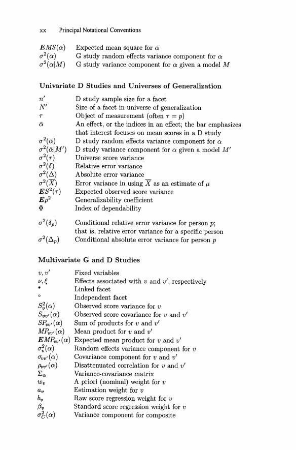
xx Principal Notational Conventions

E MS (Ci )(72(Ci)(72 (Ci1M)

Expected mean square for CiG study random effects variance component for CiG st udy variance component for Ci given a model M

Univariate D Studies and Universes of Generalization

n'N'T

ä

(72 (ä)(72(ä IM' )(72 (T)(72(8)(72(ß)

(72(X )ES2(T)E p2

q,

(72(8p )

(72( ß p )

D study sample size for a facetSize of a facet in universe of generalizat ionObj ect of measurement (often T = p)An effect, or the indices in an effect; the bar emphasizesthat interest focuses on mean scores in a D st udyD study random effects variance component for CiD study variance component for Ci given a model M'Universe score varianceRelative error varianceAbsolute error varianceError variance in using X as an estimate of f..lExp ected observed score varianceGeneralizability coefficientIndex of dependability

Conditional relative error variance for person p;t hat is, relat ive error variance for a specific personConditional absolute error variance for person p

Multivariate G and D Studies

v,v'v,e•o

S;(Ci )«: (Ci)SPvv'( Ci)MPvv'( Ci)EMPvv'(Ci)(7; (Ci )(7vv' (Ci )Puv' (Ci )E",W V

avbv

ßv(7& (Ci)

Fixed variablesEffects associated with v and u", respect ivelyLinked facetIndependent facetObserved score variance for vObserved score covariance for v and V i

Sum of products for v and V i

Mean product for v and V i

Expected mean product for v and V i

Random effects variance component for vCovariance component for v and V i

Disattenuated correlation for v and V i

Variance-covariance matrixA priori (nominal) weight for vEstimation weight for vRaw score regression weight for vStandard score regression weight for vVariance component for composite

1Introduction

The pursuit of scientific endeavors necessitates careful attention to mea­surement procedures, the purpose of which is to acquire information aboutcertain attributes or characterist ics of objects. However , the informationobtained from any measurement procedure is fallible to some degree. Thisis evident even for a seemingly uncontroversial measurement procedure suchas one used to associate a numerical value (measurement) with the lengthof an object . Clearly, the measurements obt ained may vary depending onnumerous condit ions of measurement, such as the ruler used, the personwho records the measurement , lighting conditions, and the like.

Although all measurements are fallible to some extent, scientists seekways to increase the precision of measurement. To do so, they frequentlyaverage measurements over some subset of predefined conditions of mea­surement. This average measurement serves as an est imate of the "ideal"measurement th at would be obtained (hypothetically) by averaging overall predefined condit ions of measurement. A substantive question thenbecomes, "How many instances of which conditions of measurement areneeded for acceptably precise measurement?" For example, if prior researchhas demonstrated th at the choice of ruler has little influence on measure­ments of th e length of certain objects, but considerable variability is as­sociated with the persons who record measurements, then it is sensible toavet age measurements over many persons but few rulers.

Another way that scientists sometimes increase the precision of mea­surement is to fix one or more conditions of measurement . For example, aspecific ruler might be used to obtain all measurements of the length of anobject . However, the choice of a specific ruler for all measurements involves

2 1. Introduction

a restrietion on the set of measurement conditions to which generalizationis intended. In other words , fixing a condition of measurement reduces errorand increases the precision of measurements, but it does so at the expenseof narrowing interpretations of measurements.

It is evident from this perspective on measurement that "error" does notmean mistake, and what constitutes error in a measurement procedure is,in part, a matter of definition. It is one thing to say that error is an inherentaspect of a measurement pro cedure; it is quite another thing to quantifyerror and specify which conditions of measurement contribute to it . Doingso necessitates specifying what would constitute an "ideal" measurement(i.e., over what conditions of measurement is generalization intended) andthe conditions under which observed scores are obtained.

These and other measurement issues are of concern in virtually all areasof science . Different fields may emphasize different issues, different objects,different characteristics of objects, and even different ways of addressingmeasurement issues, but the issues themselves pervade scientific endeav­ors. In education and psychology, historically these types of issues havebeen subsumed under the heading of "reliability." Generalizability theoryliberalizes and extends traditional notions of reliability.

Broadly conceived , reliability involves quantifying the consistencies andinconsistencies in observed scores. It has been stated that "A person withone watch knows what time it is; a person with two watches is never quitesure!" This simple aphorism highlights how easily investigators can be de­ceived by having information from only one element in a larger set of inter­est, Generalizability theory enables an investigator to identify and quantifythe sources of inconsistencies in observed scores that arise, or could arise ,over replications of a measurement procedure.!

Generalizability theory offers an extensive conceptual framework and apowerful set of statistical procedures for addressing numerous measurementissues. To an extent, the theory can be viewed as an extension of classicaltest theory (see, e.g., Feldt & Brennan, 1989) through an application ofcertain analysis of variance (ANOVA) procedures to measurement issues.Classical theory postulates that an observed measurement can be decom­posed into a "true" score T and a single undifferentiated random errorterm E. As such, any single application of the classical test theory modelcannot clearly differentiate among multiple sources of error. By contrast,when Fisher (1925) introduced ANOVA, he

revolutionized statistical thinking with the concept of the fac­torial experiment in which the conditions of observation areclassified in several respects. Investigators who adopt Fisher'sline of thought must abandon the concept of undifferentiated

1Brennan (in press) provides an extensive consideration of reliability from the per­spective of replications.

1. Introduction 3

error. The error formerly seen as amorphous is now at t ributedto multiple sources, and a suitable experiment can estimate howmuch variation arises from each controllable source (Cronb achet al., 1972, p. 1).

Generalizability th eory liberalizes classical theory by employing ANOVAmethods th at allow an investigator to unt angle mult iple sources of errorthat cont ribute to the undifferentiated E in classical theory

The defining tr eatment of generalizability theory is a book by Cronb achet al. (1972) ent it led The Dependability 01 Behavioral Measurement s. Ahistory of the theory is provided by Brennan (1997). In discussing thegenesis of the theory, Cronbach (1991, pp. 391- 392) states:

In 1957 I obtained funds from the Nation al Institute of Men­t al Health to produce, with Gleser's collaborat ion, a kind ofhandbook of measurement theory.. .."Since reliability has beenstudied thoroughly and is now understood," I suggested to theteam, "let us devote our first few weeks to out lining th at sectionof the handb ook, to get a feel for the undert aking." We learnedhumility th e hard way-the enterprise never got past th at topic.Not until 1972 did the book appear .. . th at exhausted our find­ings on reliability reinterpreted as generalizability. Even then,we did not exhaust the topic.

When we tri ed init ially to summarize prominent , seeminglytransparent , convincingly argued papers on test reliability, themessages conflicted.

To resolve these conflicts, Cronbach and his colleagues devised a richconcept ual framework and marri ed it to analysis of random effects variancecomponents . The net effect is "a tapestry th at interweaves ideas from atleast two dozen aut hors" (Cronbach, 1991, p. 394). In particular , Burt(1936), Hoyt (1941), Ebel (1951), and Lindquist (1953, Chap. 16) discussedANOVA approaches to reliability. Indeed, the work by Burt and Lindquistappears to have ant icipated the development of generalizability theory.

The essential features of univariate generalizability th eory were largelycompleted with technical reports in 1960-1961. These were revised intothree journal art icles, each with a different first author (Cronbach et al. ,1963; Gleser et al., 1965; and Rajaratn am et al., 1965).

In the mid 1960s, motivated by Harinder Nanda's studies on interbat ­tery reliability, th e Cronbach team began their development of multivari­ate generalizability theory, which is incorporated in their 1972 monograph .Cronb ach (1976) provides some additional perspectives.

Since the Cronbach et al. (1972) monograph , a number of publicationshave been substant ially devoted to explicat ing the theory at various levelsof detail and complexity. Für example, Brennan (1983, 1992a) provides amonograph on generalizability th eory that is quit e extensive but st ill less

4 1. Introduction

detailed than Cronbach et al. (1972). Shavelson and Webb (1991) providean introductory monograph, and Cardinet and Tourneur (1985) providea monograph in French. Shorter treatments of generalizability theory aregiven by Algina (1989), Brennan and Kane (1979), Crocker and Algina(1986), Feldt and Brennan (1989), and Strube (2000). Brief introductionsare provided by Anal (1988, 1990), Brennan (1992b), Rentz (1987), andShavelson and Webb (1992). In addition, Brennan (2000a) treats concep­tual issues, including misconceptions. Also, overviews of the theory areincorporated in Shavelson and Webb's (1981) review of the generalizabil­ity theory literature from 1973 to 1980, and in the Shavelson et al. (1989)coverage of additional contributions in the 1980s.

1.1 Framework of Generalizability Theory

Although classical test theory and ANOVA can be viewed as the parentsof generalizability theory, the child is both more and less than the simpleconjunction of its parents, and appreciating generalizability theory requiresan understanding of more than its lineage (see Figure 1.1). For example,although generalizability theory liberalizes classical test theory, not all as­pects of classical theory, as explicated by Feldt and Brennan (1989), areincorporated in generalizability theory. Also, not an of ANOVA is relevantto generalizability theory; indeed, some perspectives on ANOVA are incon­sistent with generalizability theory. In addition, the ANOVA issues empha­sized in generalizability theory are different from those that predominate inmany experimental design and ANOVAtexts. In particular, generalizabilitytheory concent rates on variance components and their estimation.

Perhaps the most important aspect and unique feature of generalizabil­ity theory is its conceptual framework. Among the concepts are universes0/ admissible observations and G (generalizability) studies , as wen as uni­uerses 0/ generalization and D (decision) studies. The concepts and themethods of generalizability theory are introduced next using a hypotheticalscenario involving the measurement of writing proficiency. As illustrated bythis scenario , generalizability analyses are useful not only for understand­ing the relative importance of various sources of error but also for designingefficient measurement procedures.f

2This hypothetical scenario is a somewhat revised version of Brennan (1992a) , whichis reprinted here with permission ofthe publisher, the National Council on Measurementin Education.

Classicaltest theory

1.1 Framework of Generalizabiiity Theory 5

Analysisof vari ance

~ .>r----------,

GeneralizabilityTheory

ConceptualIssues:

Universe of admissibleobservation and G study;Universe of generalizat ion

and D study

Statistical Issues:

Variance componentsError variances

Coefficients and indices

FIGURE 1.1. Parents and conceptuai framework of generalizabiiity theory.

1.1.1 Universe of Admissible Observations and G Studies

Suppose an invest igator, Mary Smith, decides that she wants to const ructone or more measurement procedures for evaluating writing proficiency.She might proceed as folIows. First she might identify, or otherwise char­acterize, essay prompts that she would consider using, as weIl as potenti alraters of writing proficiency. At this point, Smith is not committing herselfto actually using, in a particular measurement procedure, any specific itemsor rat ers- or , for that mat ter , any specific number of items or rat ers. She ismerely characterizing t he facets of measurement that might inte rest her orother investigators. A facet is simply a set of similar condit ions of measure­ment. Specifically, Smith is saying that any one of the essay prompts con­stitutes an admissible (i.e., acceptable to her) condition of measurement forher essay-prompt facet . Similarly, any one of the rat ers const it utes an ad­missible condition of measurement for her rat er facet . We say t hat Smith'suniverse of admis sible observat ions contains an essay-prompt facet and arater facet .

Fur thermore, suppose Smith would accept as meanin gful to her a pairingof any rater (r) with any prompt (t) . If so, Smith's universe of admissibleobservat ions would be described as being crossed , and it would be denotedt x r , where the "x" is read "crossed with." Specifically, if t here were Ntprompts and N; raters in Smit h's universe, t hen it would be described ascrossed if any one of the NtNr combinat ions of conditions from t he two

6 1. Introduction

facets would be admissible for Smith. Here, it is assumed that Nt and N;are both very large (approaching infinity, at least theoretically).

Note that it is Smith who decides which prompts and which raters consti­tute the universe of conditions for the prompt and rater facets, respectively.Generalizability theory does not presume that there is some particular def­inition of prompt and rater facets that all investigators would accept. Forexample , Smith might characterize the potential raters as college instruc­tors with a Ph .D. in English, whereas another investigator might be con­cerned about a rater facet consisting of high school teachers of English . Ifso, Smith's universe of admissible observations may be of little interest tothe other investigator. This does not invalidate Smith's universe, but it doessuggest that other investigators need to pay careful attention to Smith'sstatements about facets if such investigators are to judge the relevance ofSmith's universe of admissible observations for their own concerns.

In the above scenario, no explicit reference has been made to persons whorespond to the essay prompts in the universe of admissible observations.However, Smith's ability to specify a meaningful universe of prompts andraters is surely, in some sense, dependent upon her ideas about a popula­tion of examinees for whom the prompts and raters would be appropriate.Without some such notion, any characterization of prompts and ratersas "admissible" seems vague, at best. Even so, in generalizability theorythe word universe is reserved for conditions of measurement (prompts andraters, in the scenario), while the word population is used for the objectsof measurement (persons, in this scenario).

Presumably, Smith would accept as admissible to her the response ofany person in the population to any prompt in the universe evaluated byany rater in the universe. If so, the population and universe of admissibleobservations are crossed, which is represented p x (t x r), or simply p x t x r .For this situation, any observable score for a single essay prompt evaluatedby a single rater can be represented as:

X pt r = J.l + IIp + IIt + IIr + IIpt + Vin: + IItr + IIptr, (1.1)

where J.l is the grand mean in the population and universe and 11 designatesany one of the seven uncorrelated effects, or components, for this design."

The variance of the scores given by Equation 1.1, over the population ofpersons and the conditions in the universe of admissible observations is:

That is, the total observed score variance can be decomposed into sevenindependent variance components. It is assumed here that the populationand both facets in the universe of admissible observations are quite large

3 Actually, the effect ptr is a residual effect involving the tripIe interaction and all othersources of error not explicitly represented in the universe of admissible observations.

1.1 Framework of Generalizability Theory 7

TABLE 1.1. Expected Mean Squares and Estimators of Variance Componentsfor p x t x r Design

Effect(o:) EMS(o:)

p (J2(ptr) + nt(J2(pr) + nr(J2(pt) + ntnr(J2(p)

t (J2(ptr) + np(J2(tr) + nr(J2(pt) + npnr(J2(t)

r (J2(ptr) + np(J2(tr) + nt(J2(pr) + npnt(J2(r)

pt (J2(ptr) + nr(J2(pt)

pr (J2(ptr) + nt(J2(pr)

tr (J2(ptr) + np(J2(tr)

ptr (J2(ptr)

Effect(o:) &2(0:)

P [MS(p) - MS(pt) - MS(pr) +MS(ptr)]jntnr

t [MS(t) - MS(pt) - MS(tr) + MS(ptr)]jnpnr

r [MS(r) - MS(pr) - MS(tr) + MS(ptr)]jnpnt

pt [MS(pt) - MS(ptr)]jnr

pr [MS(pr) - MS(ptr)]jnt

tr [MS(tr) - MS(ptr)]jnp

ptr MS(ptr)

Note . Cl! represents any one of the effects .

(approaching infinity, at least theoretically) . Under these assumptions, thevariance components in Equation 1.2 are called random effects variancecomponents. It is important to note that they are for single person-prompt­rater combinations, as opposed to average scores over prompts andjorraters, which fall in the realm of D study considerations.

Now that Smith has specified her population and universe of admissibleobservations, she needs to collect and analyze data to estimate the variancecomponents in Equation 1.2. To do so, Smith conducts a study in which, letus suppose, she has a sample of n r raters use a particular scoring procedureto evaluate each of the responses by a sample of np persons to a sampleof nt essay prompts. Such a study is called a G (generalizability) study.The design of this particular study (i.e., the G study design) is denotedp x t x r . We say this is a two-facet design because the objects of mea­surement (persons) are not usually called a "facet." Given this design, theusual procedure for est imat ing the variance components in Equation 1.2

8 1. Introduction

employs the expected mean square (EMS) equations in Table 1.1. The re­sulting estimators of these variance components, in terms of mean squares,are also provided in Table 1.1. These so-called "ANOVA" estimators arediscussed extensively in Chapter 3.

Suppose the following estimated variance components are obtained fromSmith's G study.

&2(p) = .25,a-2(pt ) = .15,

and

(1.3)

These are estimates of the actual variances (parameters) in Equation 1.2.For example, a- 2 (p) is an estimate of the variance component a 2 (p), whichcan be interpreted roughly in the following manner. Suppose that, for eachperson in the population, Smith could obtain the person's mean score (tech­nically, "expected" score) over all Nt essay prompts and all N; raters inthe universe of admissible observations. The variance of these mean scores(over the population of persons) is a2 (p). The other "main effect" variancecomponents for the prompt and rater facets can be interpreted in a similarmanner. Note that for Smith's universe of admissible observations, the es­timated variance attributable to essay prompts, &2(t) = .06, is three timesas large as the estimated variance attributable to raters, a-2 (r ) = .02. Thissuggests that prompts differ much more in average difficulty than ratersdiffer in average stringency.

Interaction variance components are more difficult to describe verbally,but approximate statements can be made . For example, &2(pt) estimatesthe extent to which the relative ordering of persons differs by essay prompt,and &2(pr) estimates the extent to which persons are rank ordered differ­ently by different raters. For the illustration considered here, it is espe­cially important to note that a-2 (pt ) = .15 is almost four times as largeas a- 2 (pr) = .04. This fact, combined with the previous observation that&2(t) is three times as large as a-2(r ), suggests that prompts are a consid­erably greater source of variability in persons' scores than are raters. Theimplication and importance of these facts becomes evident in subsequentsections .

1.1.2 Infinite Universe 0/ Generalization and D Studies

The purpose of a G study is to obtain estimates of variance componentsassociated with a universe of admissible observations. These estimates canbe used to design efficient measurement procedures for operational use andto provide information for making substantive decisions about objects ofmeasurement (usually persons) in various D (decision) studies. Broadlyspeaking, D studies emphasize the estimation, use, and interpretation of

1.1 Framework of Genera lizabiiity Theory 9

variance components for decision-making with well-specified measurementprocedures.

Perhaps the most important D st udy considerat ion is the specificationof a universe of generalization, which is the universe to which a decision­maker wants to generalize based on the results of a particular measurementprocedure. Let us suppose that Smith's universe of generalizat ion containsall the prompts and rat ers in her universe of admissible observations. Sinceboth facets are assumed to be infinite, Smith's universe of generalizationwould be called "infinite" as well. In t his scenario , then, it is assumed thatSmith wants to generalize persons' scores based on t he specific promptsand raters in her measurement procedure to these persons ' scores for auniverse of generalization that involves many other prompts and raters. Inanalysis of variance terminology, such a model is described as random, andsometimes the prompt and rater facets are said to be random, too.

The universe of generalization is closely related to replications of themeasurement procedure. Let us suppose that Smith decides to design hermeasurement procedure such that each person will respond to n~ essayprompts, with each response to every prompt evaluated by the same n~

raters. Fur thermore, assurne that decisions about a person will be basedon his or her mean score over t he n~n~ observations associate d with theperson. This is a verbal description of a D st udy p x T x R design. It ismuch like t he p x t x r design for Smith's G st udy, but t here are someimportant differences.

First , the sample sizes for the D study (n~ and n~) need not be thesame as the sam ple sizes for the G study (nt and nr ) . This distinction ishighlighted by the use of primes with D study sample sizes. Second , forthe D st udy, interest focuses on mean scores for persons, rather than singleperson-promp t-ratet observat ions that are the focus of G study est imatedvariance components . This emphasis on mean scores is highlight ed by theuse of upp ercase let ters for t he facet s in Smith's D st udy p x T x R design .

Let us suppose t hat Smith decides t hat a replication of her measurementprocedure would involve a different sample of n~ essay prompts and a dif­ferent sarnple of n~ raters. Such measurement procedures are described as"randomly parallel." Th ese randomly parall el replications span the ent ireuniverse of generaliz ation, in the sense that the replications exhaust allconditions in the universe.

Universe Scores

In principle, for any person , Smith can conceive of obtaining the person 'smean score for every inst ance of the measurement procedure in her universeof generalization. For any such person , the expected value of these meanscores is th e person's universe score.

10 1. Introduction

The variance of universe scores over all persons in the population iscalled universe score variance. It has conceptual similarities with true scorevariance in classical test theory.

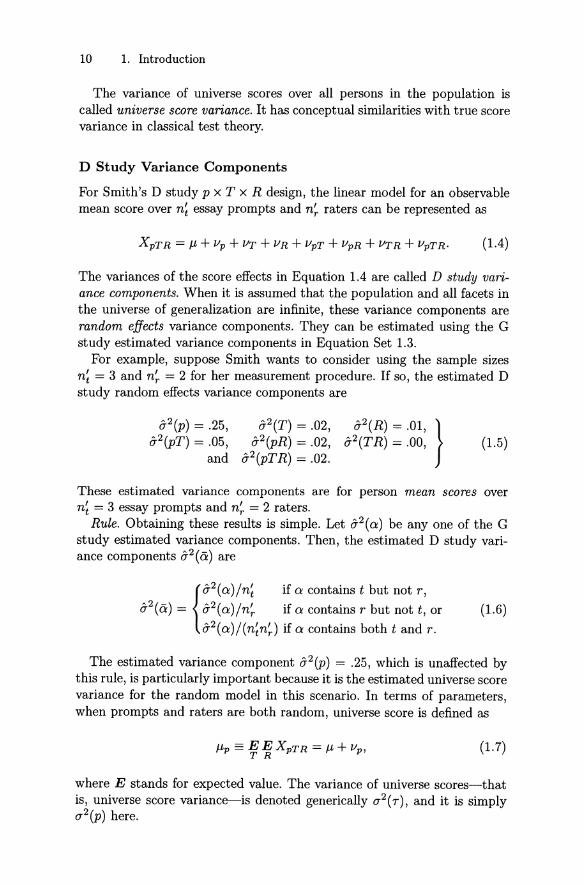
D Study Variance Components

For Smith's D study p x T x R design, the linear model for an observablemean score over n~ essay prompts and n~ raters can be represented as

XpTR = J.L + I/p + I/T + I/R + I/pT + I/pR + I/TR + I/pTR· (1.4)

The variances of the score effects in Equation 1.4 are called D study vari­ance components. When it is assumed that the population and all facets inthe universe of generalization are infinite, these variance components arerandom effects variance components. They can be estimated using the Gstudy estimated variance components in Equation Set 1.3.

For example, suppose Smith wants to consider using the sampIe sizesn~ = 3 and n~ = 2 for her measurement procedure. If so, the estimated Dstudy random effects variance components are

a-2(p) = .25,a-2 (pT ) = .05,

and(1.5)

These estimated variance components are for person mean scores overn~ = 3 essay prompts and n~ = 2 raters.

Rule. Obtaining these results is simple. Let a-2(0') be any one of the Gstudy estimated variance components. Then, the estimated D study vari­ance components a-2 (ö) are

{a-2 (0') /n~ if 0' contains t but not r,

a-2(ö) = a-2(0')/n~ if 0' contains r but not t , or

a-2(0')/ (n~n~) if 0' contains both t and r .

(1.6)

The estimated variance component a-2(p) = .25, which is unaffected bythis rule, is particularly important because it is the estimated universe scorevariance for the random model in this scenario. In terms of parameters,when prompts and raters are both random, universe score is defined as

J.Lp == E E XpTR = J.L + I/p,T R

(1.7)

where E stands for expected value. The variance of universe scores-thatis, universe score variance-is denoted generically a2(r) , and it is simplya 2 (p) here.

1.1 Framework of Generalizability Theory 11

TABLE 1.2. Random Effects Variance Components that Enter 0-2(r) , 0-2(8), and0-2(~) for p X T X R Design

D Studios"

T , R Random T Fixed

(J2(p)(J2(T) = (J2(t) /n~

(J2(R) = (J2(r) /n~

(J2(pT) = (J2(pt)/ n~(J2(pR) = (J2 (pr)/n~

(J2(TR) = (J 2(tr) /n~n~

(J2(pTR) = (J2(ptr) /n~n~

a r is univers e score.

Error Variances

T

T

ß, <5

ßß , <5

Given Smith's infinite universe of generalizat ion, vari ance components otherthan (J2(p) cont ribute to one or more different typ es of error variance. Con­sidered below are "absolute" and "relat ive" error variances.

Absolute error variance (J2(ß). Absolute error is simply the differencebetween a person's observed and universe score:

(1.8)

For this scenario , given Equat ions 1.4 and 1.7,

(1.9)

Consequently, t he variance of th e absolute errors 0-2(ß) is the sum of all thevariance components except (J2(p) . This result is also provided in Table 1.2under th e column headed "T, R Random. "

Given th e est imated D st udy variance components in Equation Set 1.5,the est imate of (J2(ß) for three prompts and two raters is:

a2(ß ) = .02 + .01 + .05 + .02 + .00 + .02 = .12,

and its square root is a(ß) = .35, which is interpretable as an est imate ofthe "absolute" stand ard error of measurement (SEM) . Consequently, withthe usual caveats, X pT R ± .35 const it utes a 68% confidence interval forpersons ' universe scores.

Suppose Smith judged a(ß) = .35 to be unacceptably large for her pur­poses, or suppose she decided th at tim e const raints preclude using threeprompts. For either of th ese reasons, or other reasons, she may want toest imate a(ß) for a number of different values of n~ and/or n~. Doing sois simple. Smith merely uses the rule in Equ at ion 1.6 to esti mate the D

12 1. Introduction

0.65 0.854

0.60 0.80 3

W; 0.752

~ 0.55 'öw ~ 0.70~ 0.50

10

e o~ 0.45

~0.65

r.l!! ~0.60:::lCi 0.40 .!:!

'" eO.55.0

~ 0.35CDc~ 0.50

0.30 20.453

0.25 4 0.402 3 4 2 3 4

Number01 Prompts Number01 Prompts

FIGURE 1.2. o-(t.) and Eß2 for scenario with p x T x R design.

study variance components for any pair of D study sam ple sizes of interestto her . Then, as indicated in Table 1.2, she sums all the estimated variancecomponents except O'2 (p), and takes the square root.

The left-hand panel of Figure 1.2 illustrates results for both n~ and n~

ranging from one to four. It is evident from Figure 1.2 that increasing n~

and/or n~ leads to a decrease in O'(Ö) . This result is sensible, since averag­ing over more conditions of measurement should reduce error. Figure 1.2also suggests that using more than three raters leads to only a very slightreduction in O'(Ö) . Consequently, probably it would be unnecessary to usemore than three raters (and perhaps only two) for an actual measurementprocedure. In addition, Figure 1.2 indicates that using additional promptsdecreases O'(Ö) quicker than using additional raters. This is a direct resultof the fact that O'2(t ) = .06 is larger than O'2(r ) = .02, and O'2(pt ) = .15 islarger than O'2 (pr ) = .04. Consequently, for this example, all other thingsbeing equal, it would seem desirable to use as many prompts as possible.

Relative error variance (j2 (8). Relative error is defined as the differ­ence between a person's observed deviation score and his or her universedeviation score:

8p == (XpTR - J.LTR) - (J.Lp - J.L), (1.10)

where J.LTR is the expected value over persons of the observed scores X pTRfor the p x T x R design . It can be shown that

(1.11)

and the variance of these relative errors is the sum of the variance com­ponents for the three effects in Equation 1.11. This result is also given inTable 1.2, under the eolumn headed "T, R Random." Relative error vari­anee is similar to error variance in classical theory.

For the example introduced previously, if n~ = 3 and n~ = 2, then

0'2(8) = .05 + .02 + .02 = .09,

1.1 Framework of Generalizability Theory 13

and its square root is &(6) = .30, which is interpretable as an estimate ofthe "relative" SEM. Note that this value of &(6) is smaller than &(ß) = .35for the same pair of sampie sizes. In general, &(6) is less than &(ß) because,as indicated in Table 1.2, &2(6) involves fewer variance components than&2(ß) . In short, relative interpretations about persons' scores are less errorprone than absolute interpretations.

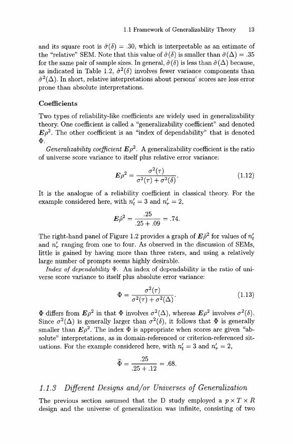
Coefficients

Two types of reliability-Iike coefficients are widely used in generalizabilitytheory. One coefficient is called a "generalizability coefficient" and denotedE p2. The other coefficient is an "index of dependability" that is denotedif>.

Generalizability coefficient E p2. A generalizability coefficient is the ratioof universe score variance to itself plus relative error variance:

(1.12)

(1.13)

It is the analogue of a reliability coefficient in classical theory. For theexample considered here , with n~ = 3 and n~ = 2,

, 2 .25Ep = .25 + .09 = .74.

The right-hand panel of Figure 1.2 provides a graph of E{J2 for values of n~

and n~ ranging from one to four. As observed in the discussion of SEMs,little is gained by having more than three raters , and using a relativelylarge number of prompts seems highly desirable .

Index 01 dependability if>. An index of dependability is the ratio of uni­verse score variance to itself plus absolute error variance:

if> _ (7"2(7)- (7"2(7) + (7"2(ß)"

if> differs from E p2 in that if> involves (7"2 (ß), whereas E p2 involves (7"2 (6).Since (7"2 (ß) is generally larger than (7"2 (6), it follows that if> is generallysmaller than E p2 . The index if> is appropriate when scores are given "ab­solute" interpretations, as in domain-referenced or criterion-referenced sit­uations. For the example considered here, with n~ = 3 and n~ = 2,

if> = .25 = .68..25 + .12

1.1.3 Different Designs and/or Universes of Generalization

The previous section assumed that the D study employed a p x T x Rdesign and the universe of generalization was infinite, consisting of two

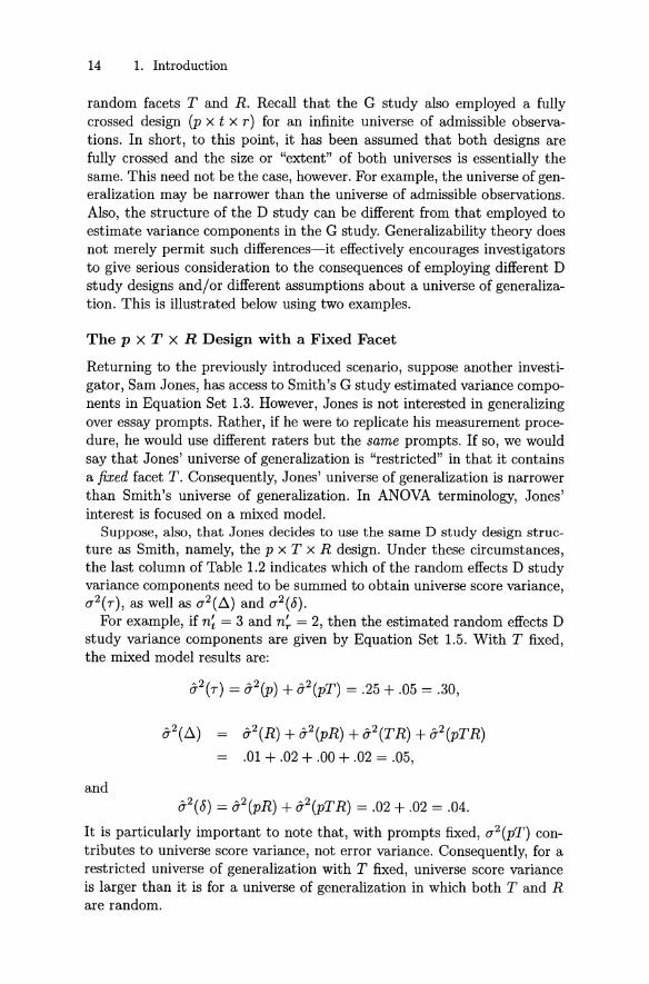
14 1. Introduction

random facets T and R. Recall that the G study also employed a fullycrossed design (p x t x r) for an infinite universe of admissible observa­tions. In short, to this point, it has been assumed that both designs arefully crossed and the size or "extent" of both universes is essentially thesame. This need not be the case, however. For example, the universe of gen­eralization may be narrower than the universe of admissible observations.Also, the structure of the D study can be different from that employed toestimate variance components in the G study. Generalizability theory doesnot merely permit such differences-it effectively encourages investigatorsto give serious consideration to the consequences of employing different Dstudy designs and/or different assumptions about a universe of generaliza­tion. This is illustrated below using two examples .

The p X T X R Design with a Fixed Facet

Returning to the previously introduced scenario, suppose another investi­gator, Sam Jones, has access to Smith's G study estimated variance compo­nents in Equation Set 1.3. However, Jones is not interested in generalizingover essay prompts. Rather, if he were to replicate his measurement proce­dure , he would use different raters but the same prompts. If so, we wouldsay that Jones' universe of generalization is "restricted" in that it containsa fixed facet T . Consequently, Jones' universe of generalization is narrowerthan Smith's universe of generalization. In ANOVA terminology, Jones'interest is focused on a mixed model.

Suppose, also, that Jones decides to use the same D study design struc­ture as Smith, namely, the p x T x R design. Under these circumstances,the last column of Table 1.2 indicates which of the random effects D studyvariance components need to be summed to obtain universe score variance,(12(7), as weIl as (12(ß) and (12(8).

For example, if n~ = 3 and n~ = 2, then the estimated random effects Dstudy variance components are given by Equation Set 1.5. With T fixed,the mixed model results are:

0-2(R) + 0-2(pR) + 0-2(TR)+ 0-2(pTR)

.01 + .02 + .00 + .02 = .05,

and0-2(8) = 0-2(pR) + 0-2(pTR) = .02 + .02 = .04.

It is particularly important to note that, with prompts fixed, (12(pT) con­tributes to universe score variance, not error variance. Consequently, for arestricted universe of generalization with T fixed, universe score varianceis larger than it is for a universe of generalization in which both T and Rare random.

1.1 Framework of Generalizability Theory 15

Given th ese results, it follows from Equation 1.12 th at

EfJ2 = .30 = .88..30 + .04

Recall that , for these D study sampIe sizes (n~ = 3 and n~ = 2), whenprompts were considered random , Smith obt ained EfJ2 = .74. The esti­mated generalizability coefficient is larger when prompts are consideredfixed because a universe of generalization with a fixed facet is narrowerthan a universe of generalization with both facets random. That is, gener­alizations to narrow universes are less error prone th an generalizations tobroader universes. It is important to note, however, this does not necessar­ily mean th at narrow universes are to be preferred, because restricting auniverse also restricts the extent to which an investigator can generalize.For example, when prompts are considered fixed, an investigator cannotlogically draw inferences about what would happen if different promptswere used.

The p X (R:T) Design

To expand our scenario even further , consider a third investigator, AnnHall, who decides that practical const raints preclude her from having allraters evaluate all responses of all persons to all prompts. Rather, shedecides that , for each prompt, a different set of raters will evaluate persons 'responses. This is a verbal description of the D study p x (R :T) design,where ":" is read "nested within ." For this design, the total variance is thesum of five independent variance components ; th at is,

(1.14)

(1.15)

For a random effects model, these variance components can be est imatedusing Smith's est imated G study variance components , even though Smith 'sG study design is fully crossed, whereas Hall's D study design is parti allynested. The process of doing so involves two steps.

First , the G study variance components for the p x (r :t ) design are es­t imated using the results in Equation Set 1.3 for the p x t x r design. Forboth designs, a-2(p) = .25, a-2(t ) = .06, and a-2(pt ) = .15. Formulas for est i­mating the remaining two G study variance components for the p x (r :t)design are:

anda-2 (pr:t ) = a-2 (pr ) + a-2(ptr ), (1.16)

which give a-2 (r:t ) = .02 + .00 = .02, and a-2 (pr:t ) = .04 + .12 = .16.Second, the rule in Equat ion 1.6 is applied to th e est imated G study

variance components for the p x (r :t) design. Assuming n~ = 3 and n~ = 2,

16 1. Introduction

TABLE 1.3. Random Effects Variance Components that Enter (72(r), (72(8), and(72(ß) for p X (R :T) Design

D Studies"

T ,R Random T Fixed

(72(p)a2(T) = (72(t)/n~

a2(R:T) = a2(r:t)/n~n~

a2(pT) = a2(pt)/n~

a2(pR:T) = a2(pr:t)/n~n~

ar is universe score.

the results are :

7

7

6 ,8

0-2(p) = .250, 0-2(T) = .020, 0-2(pT) = .050, } (1.17)0-2(R:T ) = .003, and 0-2(pR: T) = .027.

The second column in Table 1.3 specifies how to combine the est imatesin Equation Set 1.17 to obtain 0-2(7), 0-2(6 ) , and 0-2(8) for a universe ofgeneralization in which both T and R are random. The third column applieswhen prompts are fixed. Once 0-2(7), 0-2(6 ), and 0-2(8) are obtained, E p2and <I> can be estimated using Equations 1.12 and 1.13, respectively.

Suppose, für example, that Hall decides to generalize to a universe inwhich both T and Rare considered random. For thi s universe of general­ization,

0-2(T) + 0-2(pT) + 0-2(R:T) + 0-2(pR:T)

.020 + .050 + .003 + .027 = .100,

and0-2(8) = 0-2(pT) + 0-2(pR: T) = .050 + .027 = .077.

It follows t hat

.250---- = .76..250 + .077

Recall that for the p x T x R design with T and R random, Smith ob­tained Eß2 = .74, which is somewhat different from E ß2 = .76 for the sameuniverse using the p x (R:T) design. The difference in t hese two results isnot rounding error. Rather, it is att ributable to the fact t hat 0- 2(8) = .090for the p x T x R design is larger t han 0-2 (8) = .077 for the p x (R :T) de­sign . This illustrates that reliability, or generalizability, is affected by design

1.1 Framework of Generalizability Theory 17

st ruct ure. Recall t hat it has been demonst rated previously t hat reliability,or generalizability, is also affected by sampie sizes and t he size or "ex­tent" of a universe of generalizat ion. T hese results illust rate an importantfact: name ly, it can be very mislead ing to refer to the reliability or the er­ror variance of a measurement procedure without considerable explanationand qualification.

1.1.4 Other Issues and Applications

All ot her things being equal, the power of generalizability theory is mostlikely to be realized when a G st udy employs a fully crossed design and alarge sampie of condit ions for each facet in the universe of admissible obser­vations. A large sampie of condit ions is beneficial because it leads to morestable est imates of G st udy variance components . A crossed design is ad­vantageous because it maximizes the numb er of design structures that canbe considered for one or more subsequent D studies. However, any designst ruct ure can be used in a G st udy. For example, the hypothetic al scenariocould have used a G st udy p x (r: t ) design , but t hen an investig ator couldnot est imate all variance components for a D st udy p x T x R design.

It often happ ens t hat the dist inction between a G and D st udy is blurred,usually because the only available data are for an operational administ ra­tion of an act ual measurement procedure. In this case, the procedures dis­cussed can st ill be followed to est imate parameters such as erro r variancesand generalizability coefficients , but obviously under these circumstancesan investigator cannot take advantage of all aspects of generalizability t he­ory.

In most applicat ions of generalizability theory, examinees or persons aret he objects of measurement . Occasionally, however, some ot her collectionof condit ions plays t he role of objec ts of measurement. For example, inevaluat ion st udies, classes are often the objects of measurement with per­sons and ot her facets being associated with t he universe of generalizat ion.It is st raight forward to apply generalizability theory in such cases.

Generalizability theory has broad applicability and has been applied innumerous sett ings. Some real-dat a examples are provided in this book ,but these are only a few illustrations. The theory has been applied to avast array of educat ional tests and to a wide range of ot her typ es of tests,including foreign language tests (e.g., Bachman et al., 1994), personalitytests (e.g., Knight et al., 1985), psychological inventories (e.g., Crowleyet al., 1994), career choice instruments (e.g., Hartm an et al., 1988), andcognitive ab ility tests (e.g., T hompson & Melancon, 1987).

Other areas of applicat ion include perform ance assessments in educa­t ion (e.g., Linn & Bur ton , 1994), standard set ti ng (e.g., Brennan , 1995b;Norcini et al., 1987), st udent rat ings of instruction (e.g., Crooks & Kane,1981), teac hing behavior (e.g., Shavelson & Dempsey-Atwood , 1976), mar­keting (e.g., Finn & Kayande, 1997), business (e.g., Marcoulides , 1998), job

18 1. Introduction

analyses (e.g., Webb & Shavelson, 1981), survey research (e.g., Johnson &Bell, 1985), physical education (e.g., Tobar et al., 1999), and sports (e.g.,Oppliger & Spray, 1987).

Generalizability theory has also been used in numerous medical areas tost udy matters such as sleep disorders (e.g., Wohlgemuth et al., 1999), clini­cal evaluations (e.g., Boodoo & O'Sullivan, 1982), nursing (e.g., Butterfieldet al., 1987), dental educat ion (e.g., Chambers & Loos, 1997), speech per­cept ion (e.g., Demorest & Bernstein, 1993), biofeedback (e.g., Hat ch et al.,1992), epidemiology (e.g., Klipst ein-Grobusch et al. , 1997), ment al retar­dat ion (e.g., Ulrich et al., 1989), and computerized scoring of performanceassessments (e.g., Clauser et al., 2000).

1.2 Overview of Book

The hypothet ical scenario used in Section 1.1 is clearly idealized and in­complete , but it does highlight many of the most important and frequentlyused concepts and procedures in generalizability theory. The remainingchapters delve more deeply into th e conceptual and statistical details andextend the theory in various ways.

This book is divided into three sets of chapte rs that are ordered in termsof increasing complexity. The fundamentals of univariate genera lizabilitytheory are contained in Chapters 1 to 4. The scope of these chapte rs isa sufficient basis for performing many generalizability analyses and forunderstanding much of the current literature on generalizability theory.Additional, more challenging topics in univariate theory are covered inChapters 5 to 8. These chapters are devoted largely to stati stical complex­ities such as the variability of est imated variance components and est imat­ing variance components for unbalanced designs. Finally, Chapters 9 to 12cover multivariate generalizability theory, in which each object of measur e­ment has multiple universe scores. In these chapte rs, particular attent ionis given to tables of specifications for educat ional and psychological tests.

This book is intended to be both a textbook and a resource for practition­ers. To serve these dual purposes, most chapters involve four components:a discussion of theory, one or more synthet ic data examples, a few real-dat aexamples, and exercises. Detailed answers to st arred exercises are given inAppendix I; answers to the remaining exercises are available from the au­thor (robert -brennan@uiowa.edu) or the publisher (www.springer-ny.com).Someti mes the four components are split over two chapte rs, and not all top­ics in all chapters are illustrated with real-data examples, but the four-waycoverage predominates.

The real-dat a examples are intended to be instructive; they are not mod­els for "ideal" generalizability analyses. Different applicat ions of generaliz­ability theory tend to involve somewhat different mixes of concept ual and

1.3 Exercises 19

statistical concerns. Consequently, a reasonable approach in one context isnot necessarily appropriate in others. Most of the real-data exampies aredrawn from the field of educational testing, but a few are from other areasof inquiry. Note, also, that Cronbach et al. (1972) provide a number ofillustrative detailed examples from psychology and education.

The synthetic data examples serve two purposes : they illustrate variousresults in a relatively simple manner, and they are sufficiently "small" topermit the reader to perform all computations with a hand-held calculator.In practical contexts, however, computer programs are required for per­forming generalizability analyses. Three computer programs are availablethat are specifically coordinated with the content of this book: GENOVA,urGENOVA, and mGENOVA. These are introduced at appropriate points.Using one or more of these programs, most of the computations discussedin this book can be performed for almost any data set.

The number of decimal digits used in the examples varies, depending onthe context. For synthetic data examples, usually four decimal digits arereported so that readers can be assured that their computations are cor­rect , at least to the next to the last decimal digit. Some real-data examplescome from published papers in which results are reported with fewer digits .Performing computations with four, five, or even more digits is to be rec­ommended so that rounding errors have mimimal impact on final results .However, reporting results with that many decimal digits does not meanthat it is necessarily reasonable to base interpretations on the magnitudeof digits far to the right of a decimal point.

Some students and practitioners who initially encounter generalizabil­ity theory are overwhelmed by the statistical issues. That is why the earlychapters of this book often sidestep statistical complexities or relegate themto exercises. Other students and practitioners have little trouble with thestatistical "hurdle," but the conceptual issues challenge them. In particu­lar , in the author's experience, persons with strong statistical backgroundsare prone to view the theory simply as the application of variance compo­nents analysis to measurement issues. There is an element of truth in sucha perspective, but variance components analysis is a tool used in general­izability theory--it does not encompass the theory. For example, variancecomponents analysis per se does not tell an investigator which componentscontribute to which type of error, and these are central issues in generaliz­ability theory.

1.3 Exercises

1.1* Suppose an investigator obtains the following mean squares for a Gstudy p x t x r design using n p = 100 persons, nt = 5 essay items (or

20 1. Introduction

tasks), and n r = 6 raters.

MS(p) = 6.20,

MS(pt) = 1.60,

and

MS(t) = 57.60,

MS(pr) = .26,

MS(ptr) = .16.

MS(r) = 28.26,

MS(tr) = 8.16,

(a) Estimate the G study variance components assuming both t andr are infinite in the universe of admissible observations.

(b) Estimate the D study random effects variance components for aD study p x T x R design with n~ = 4, n~ = 2, and with personsas the objects of measurement.

(c) For the D study design and sampie sizes in (b), estimate ab­solute error variance, relative error variance, a generalizabilitycoefficient, and an index of dependability.

(d) Estimate er(~) if an investigator decides to use the D studyp x (R:T) design with n~ = 3 and n~ = 2, assuming T and Rare both random in the universe of generalization.

1.2* Suppose an investigator specifies that a universe of generalizationconsists of only two facets and both are fixed. From the perspectiveof generalizability theory, why is this nonsensical?

1.3 Brennan (1992a, p. 65) states that, "... the Spearman-Brown Formuladoes not apply when one generalizes over more than one facet ." Ver­ify this statement using the random model example of the p x T x Rdesign in Section 1.1.2, where Eß2 = .74 with three prompts andtwo raters. Assurne the number of prompts is doubled, in which casethe Spearman-Brown Formula is 2 rel/(l + rel), where rel is reliabil­ity. Explain why the Spearman-Brown formula and generalizabilityprocedures give different results.

2Single-Facet Designs

Throughout this chapter it is assumed that th e universe of admissible obser­vations and th e universe of generalization involve condit ions from th e samesingle facet , usually referred to as an item facet. Also, it is usually assumedth at the population consists of persons. For a single-faceted universe, t hereare two designs th at might be employed in a G study: the p x i or t he i:pdesign, where th e letter pis used to index persons (or examinees) , i indexesitems, "x" is read "crossed with ," and ":" is read "nested within." For thep x i design, each person is administered th e sam e random sample of items.For th e i :p design, each person is administered a different random sampleof items. Similarly, th ere are two possible D study designs: p x l and I :p,where uppercase I is used to emphasize that D study considerat ions involvemean scores over sets of items.

The most common pairing is a G study p x i design with a D study p x Idesign. If we (verbally) neglect th e distinction between i and I , th en wecan say that the two designs are the same . This design is the subject of thefirst three sections of this chapter, which systemati cally introduce many ofthe statistical issues in genera lizability theory. These sect ions are followedby a considerat ion of th e G study i:p and D study Lip designs.

Technically, th e theory discussed in this chapter assurnes that both thepopulati on of persons and th e universe of items are infinite, which is sym­bolized as Np -> 00 and Ni -> 00 . In practice, this assumption is seldom ifever literally true, but it is a useful idealization for many studies.

22 2. Single-Facet Designs

2.1 G Study p X i Design

Let X pi denote the score for any person in the population on any item inthe universe. The expected value of a person 's observed score, associatedwith a process in which an item is randomly selected from the universe, is

(2.1)

where the symbol E is an expectation operator, and the subscript i des­ignates the facet over which the expectation is taken. The score fJ,p canbe conceptualized as an examinee's "average" or "mean" score over theuniverse of items. In a similar manner, the population mean for item i isdefined as

fJ,i == EXpi ,p

and the mean over both the population and the universe is

fJ,==EEXpi.p t

(2.2)

(2.3)

These mean scores are not observable because, for example, examineeresponses to alt items in the universe are never available. Nonetheless, anyperson-item score that might be observed (an observable score) can beexpressed in terms of fJ,p, fJ,i, and fJ, using the linear model:

J.L

+fJ,p-fJ,

+fJ,i - fJ,

+ X pi - fJ,p - fJ,i + fJ,

which can be expressed more succinctly as

(grand mean)

(person effect = IIp )

(item effect = lIi)

(residual effect = IIpi ), (2.4)

(2.5)

Equations 2.4 and 2.5 represent the same tautologies. In each of themthe observed score is decomposed into components, or effects. The onlydifference between the two equations is that in Equation 2.4 each effect isexplicitly represented as a deviation score, while in Equation 2.5 the Greekletter 11 represents an effect.! For example, the person effect is IIp = fJ,p - fJ"and the item effect is lIi = fJ,i - fJ,. The residual effect, Vpi = X pi - fJ,p - fJ,i+fJ"is sometimes referred to as the interaction effect. Actually, both verbal de­scriptions are somewhat misleading because, with a single observed scorefor each person-itern combination, the person-item interaction effect and

lCronbach et aJ. (1972) and Brennan (1992a) use J1.rv to designate a score effect. Forexample, they use J1.P rv rather than vp .

2.1 G Study p x i Design 23

all other residual effects are completely confounded (totally indistinguish­able).2

All of the effects (except f-L) in Equat ions 2.4 and 2.5 are called mndomeffects because they are associated with a process of random sampling fromthe population and universe. Under these assumpt ions, the linear model isreferred to as a random effects model. The manner in which these randomeffects have been defined implies th at

E vp = E Vi = E Vpi = E Vpi = O.P , P ,

(2.6)

Equations 2.5 and 2.6 can be used directly to express mean scores in termsof score effects. For example, given the definition of f-Lp in Equation 2.1, itfollows th at

f-L + vp + E Vi + E Vpi, ,(2.7)

Similarly,(2.8)

To this point, the words "st udy" and "design" have not been used. Thatis, the model in Equation 2.5 has been defined without explicitly specifyinghow any observed data are collected. Let us now assurne that G study dataare collected in the following manner.

• A random sampie of np persons is selected from the popul ation ;

• an independent random sampie of ni items is selected from the uni­verse; and

• each of the np persons is administered each of the ni items, and t heresponses (Xpi ) are obtained.

Technically, this is a description of the G study p x i design, with the linearmodel given by Equat ion 2.5. Th at is, in a sense, Equat ion 2.5 act uallyplays two roles: it characterizes the observable data for the population anduniverse, and it represents the act ual observed data for a G stu dy.

It is "assumed" th at all effects in the model are uncorrelated. Letting aprime designate a different person or item, this means that

E(vpvp') = E(ViVi') = E(VpiVp1i) = E(VpiVpi/) = E(VpiVp1i/) = 0, (2.9)

and(2.10)

2For this reason , Cronbach et al. (1972) denote th e residu al effect as (J1,pi ~ , e).

24 2. Single-Facet Designs

The word "assumed" is in quotes because most of these zero expectationsare a direct consequence of the manner in which score effects have beendefined in the linear model and/or the random sampling assumptions forthe p x i design (see Brennan, 1994).3 For example, the random samplingassumptions imply that E(VpVi) = (Evp)(Evi) = O.

The above development can be summarized by saying that a G studyp x i design is represented by the linear model in Equation 2.5 with uncor­related score effects. This description is adequate provided it is understoodin the sense discussed above. Note, also, that the modeling has been spec­ified without any normality assumptions, and without assuming that scoreeffects are independent, which is a stronger assumption than uncorrelatedscore effects.

2.2 G Study Variance Components for p X i Design

For each score effect, or component, in Equation 2.5, there is an associ­ated variance of the score effect, or component, which is called a variancecomponent. For example, the variance component for persons is

E(fLp - E fLp)2p p

E(fLp - fL)2p

Ev;.p

(2.11)

From this derivation, it is evident that (J'2(p) might be denoted (J'2(fLp) or(J'2(vp). In other words, the variance of person mean scores is identical tothe variance of person score effects. Similarly, for items,

(2.12)

which might be denoted (J'2(fLi) or (J'2(Vi), indicating that the variance ofitem mean scores is identical to the variance of item score effects.

For the interaction of persons and items,

(J'2(pi) = E E(Xpi - fLp - fLi + fL)2 = E E V;i' (2.13)p t p t

The variance component (J'2(pi) might be denoted (J'2(Vpi)' but not (J'2(fLpi) 'Cronbach et al. (1972) denote the interaction (or residual) variance com­ponent as (J'2(pi, e) rather than (J'2(pi) . Their notation explicitly reflectsthe confounding of the interaction variance component with the varianceassociated with other residual effects or sources of "error .""

3T hese distinctions are considered more explicitly in Section 5.4.4The confounded-effects notation is not used routinely in this book, because it is

awkward for multifacet designs.

2.2 G Study Variance Components for p x i Design 25

These variance component s provide a decomposition of the so-called "to­t al" variance:

(2.14)

The derivation of Equ ation 2.14 is tedious, but no assumptions are requiredbeyond t hose in Section 2.1. T he total variance is a variance of scores forsingle persons on single items. It follows that the variance components arefor "single" scores, too .

These variance components might be concept ualized in the followingmanner. Suppose Np and Ni were very large, but still finite. Under thiscircumstance, in theory, all items in the universe could be administe red toall persons in the population. Given t he resulting observed scores, valuesfor the mean scores in Equ ations 2.1 to 2.3 could be obtained. Then (J2(p)could be compute d by taking the variance, over the population of persons,of the scores /-L p . Similarly, (J2(i) could be computed by taking the variance,over the universe of items, of the scores /-L i. Finally, (J 2(pi) could be com­puted by taking the variance, over both persons and items, of the scoresX pi - /-Lp - /-Li + /-L. This approach to interpretin g variance components isclearly a cont rived scenario, but frequentl y it is a helpful concept ual aid .

2.2.1 Estimating Variance Components

In generalizability t heory, variance components assurne cent ral importance.They are t he building blocks t hat provide a crucial foundation for all subse­quent results. To understand variance components , Equations 2.11 to 2.13are useful , but t hey cannot be used directly to estimate variance compo­nents because t hese equations are expressed in terms of squares of t he un­known random effects in the model. Rather , variance components are usu­ally est imated t hrough an analysis of variance. Table 2.1 provides ANOVAcomputational formulas for t he p x i design. Note that 0: is used in Table 2.1(and elsewhere in t his book) as a generic identifier for an effect .

To this point, all reference to mean scores has implied population and/oruniverse mean scores. Now, however , we must clearly distinguish betweenthese mean scores and t heir observed score analogues, which result from a Gstudy. For example, the mean of the observed scores for person p is denotedXp in Table 2.1, and it is t he observed score analogue of /-L p . Similarly, Xiis t he mean of the observed scores for item i, and it is analogous to tu.

Finally, X is analogous to /-L.For th e p x i design , th e derivation of the so-called "ANOVA" est ima­

tors of the variance components in Table 2.1 is rather st raight forward. Onesuch derivation is out lined next . Consider, again , Equ ation 2.4 for t he de­composition of X pi into score effects , or components. Replacing populationand/or universe mean scores with t heir observed score analogues, it is easy

26 2. Single-Facet Designs

TABLE 2.1. ANOVA Formulas and Notation for G Study p x i Design

Effect(a) df(a) SS(a) MS(a) 0-2'(a)

np -1 SS(p) MS(p) 0-2(p) = MS(p) - MS(pi)p

ni

i ni -1 SS(i) MS(i) A2C) MS(i) - MS(pi)(7 Z =

nppi (np - l)(ni - 1) SS(pi) MS(pi) 0-2(pi) = MS(pi)

to show th at

The sum of these squared observed deviation scores is

ni ~)Xp - X) 2+ np2:)Xi - X) 2p

+ L: L:(Xpi - X p - x, + X) 2. (2.15)p

Equation 2.15 provides a decomposition of the tot al sums of squares forthe p x i design into sums of squares at t ributable to persons, items, andinteractions ; th at is,

L L(Xpi - X)2 = SS(p) + SS(i) + SS(pi) .p i

The sums of squares formulas in Equation 2.15 are basic from a defini­tional perspective, but for calculation purposes the formulas reported inTable 2.1 are easier to use. For example,

and the latter formula is computationally easier to use than the former.Each sum of squares has a mean square associated with it , which is

simply the sum of squares divided by its degrees of freedom. For example,

n '" (X X)2MS(p) = t L..p p -np -1

2.2 G Study Variance Components für p x i Design 27

X pi J.t X pi = J.t

+ (J.t p - J.t ) + Vp

+ (J.ti - IL) + Vi

+ (X pi - J.tp - J.ti + J.t ) + Vp i

E MS (p) E MS (i ) E MS (pi )

FIG URE 2.1. Venn diagrams für p x i design.

To est imate varian ce components we make use of well-known equat ions forthe expected values of these mean squares (EMS equat ions):

E MS(p)

E MS(i )

E MS (pi )

(7 2(pi) + ni (72(p)

(72 (pi) +np (72 (i)

(72 (pi) .

(2.16)

(2.17)

(2.18)

Solving these equat ions for t he variance components, and using mean squaresin place of t heir expected values, we obtain the ANOVA estim ators:

0-2 (p)MS (p) - MS (pi)

(2.19)n i

0- 2(i)MS (i) - MS(pi)

(2.20)np

0-2 (pi) MS(pi). (2.21)

For the p x i design , th e equat ions for estimating variance componentscan be illustrated using a Venn diagram approach. More importantly, how­ever , Venn diagrams provide a useful visual and concept ual aid in und er­st anding variance components, as weil as other aspects of generalizabilityanalyses. The upp er left-hand corner of Figure 2.1 provides t he generalform of a Venn diagram for the p x i design , followed by the linear modelexpressions discussed in Section 2.1. The bottom half of Figure 2.1 pro­vides Venn diagram represent ations of the expected mean squares givenby Equat ions 2.16 to 2.18 . Note that circles and their intersections can be

28 2. Single-Facet Designs

TABLE 2.2. Synthetic Data Set No. 1 and the p x i Design

Item Scores (Xpi )

Person 1 2 3 4 5

1 1 0 1 0 0

2 1 1 1 0 0

3 1 1 1 1 1

4 1 1 0 1 1

5 1 1 1 1 1

6 1 1 1 0 1

7 1 1 1 1 1

8 1 1 1 1 0

9 1 1 1 1 1

10 1 1 1 1 1

Xi 1.0.9 .9 .7.7

6 7 8 9 10

o 0 0 0 0

1 0 0 0 0

o 0 0 0 0

o 0 1 0 0

o 1 0 0 0

1 1 0 0 0

1 1 0 0 0

1 1 1 1 1

1 1 1 1 1

1 1 1 1 1

.6 .6 .4 .3 .3

11 12

o 0

o 0

o 0

o 0

o 0

o 0

o 0

o 0

1 0

1 1

.2 .1

.1667

.3333

.4167

.4167

.5000

.5000

.5833

.7500

.9167

1.0000

- ",-2X = .5583 L- X p = 3.7292

pL: X~ = 4.71

tL: L: X 2 = 67p i pt

TABLE 2.3. G Study p x i Design For Synthetic Data Set No. 1

Effect(a)

Pi

pi

df(a)

9

11

99

SS(a)

7.3417

9.6917

12.5583

MS(a)

.8157

.8811

.1269

a-2 (p) = .0574

a-2 (i ) = .0754

a-2 (pi) = .1269

interpreted as expected mean squares, while parts of circles can be inter­preted as variance components, or simple functions ofthem. Note, however,that the actual areas in these diagrams are not generally proportional tothe magnitudes of the variance components. Replacing parameters withestimates, it is evident from the first and third diagrams at the bottom ofFigure 2.1 that a-2 (p) = [MS(p)-MS(pi)lfni, as indicated in Equation 2.19.

2.2.2 Synthetic Data Example

Consider Synthetic Data Set No. 1 in Table 2.2. Using the equations inSection 2.2.1, it is easy to verify the numerical values for a-2 (p), a-2 (i ), anda-2 (pi ) in Table 2.3. Readers unfamiliar with estimating variance compo­nents are encouraged to verify these results. It is evident that the estimatedvariance component for persons, a-2(p) = .0574, is slightly less than the es-

2.3 D Studies for the p x I Design 29

timated variance for items, a2(i ) = .0754, but neither of these variancecomponents is nearly as large as a2 (pi) = .1269. These variance compo­nents appear small in terms of their absolute values. However, since theyare based on dichotomous data, none of them can be larger than 0.25.

In thinking about the magnitudes of these estimated variance compo­nents, it is helpful to remember that they provide a decomposition of theestimated total variance (see Equation 2.14) of scores (0 or 1) for singlepersons on single items. In particular, a2 (i) and a2 (pi) are not estimatedvariance components for mean (or total) scores over the ni = 12 items inthe G study. However, as shown soon, a2 (pi) and sometimes a2 (i) con­tribute to estimates of several types of error variance for mean scores in aD study p x I design, and their contributions to such error variances canbe reduced by increasing the D study sampie size for items.

In Table 2.3 numerical results involving the estimation of variance com­ponents are reported to four decimal places. In part this is done to facilitatedemonstrations of certain algebraic identities. More importantly, this con­vention emphasizes that computations should be performed using as muchnumerical accuracy as possible. Generalizability analyses involve numerouscomputations, and premature rounding can distort estimates of variancecomponents. However, this convention does not mean that four digits aregenerally required for purposes of interpreting estimated variance compo­nents. Indeed, as discussed extensively in Chapter 6, estimated variancecomponents are subject to sampling variability, and when sampie sizes aresmall, such variability is likely to be large enough to cast considerable doubton the stability of third and fourth digits (or any digit, in extreme cases).

Concern about "significant" digits in estimates of variance componentsdoes not mean, however, that it is advisable to perform tests of statisti­cal significance for the estimates themselves. In generalizability theory themagnitudes of estimated variance components are of central importance,rather than their statistical significance at some preassigned level. Even ifan estimated variance component does not possess statistical significance,the ANOVA procedure yields an unbiased estimate. As such, it is better touse the estimate than to replace it by zero (Cronbach et al., 1972, p. 192).In particular, generalizability theory emphatically does not involve per­forming F tests on the ratios of mean squares. In generalizability theory,mean squares are used simply to estimate variance components.

2.3 D Studies für the p x I Design

To this point, discussion has focused on the model and associated variancecomponents for a person's score on a single item (X pi ) in the universeof admissible observations. By contrast, if an examinee is administered asampie of n; items, decisions about the examinee will be based , surely,

30 2. Single-Facet Designs

on his or her average (or total) score over the n~ items, not a score on asingle item . From the perspective of generalizability theory, the intent ofsuch adecision is to generalize from the examinee's observed score to theexaminee's universe score over all items in the universe 0/ generalization.

Another perspective on the universe of generalization is based on thenotion of replications of a measurement procedure (see Brennan, in press).From this perspective, multiple measurements of an examinee would consistof his or her average score on different random samples of n~ items fromthe same universe. Such samples of items, or test forms, are said to berandomly parallel, and for the p x I design, the universe of generalizationcan be viewed as a universe of such randomly parallel forms.

By convention, in generalizability theory, average scores over a sample ofconditions are indicated by uppercase letters. Using this notation for the Dstudy p x I design, the linear model for the decomposition of an examinee 'saverage score XpI over n~ items is

(2.22)

where XpI and X p mean the same thing. 5 Equation 2.22 is completelyanalogous to Equation 2.4, the only difference being that i (for a singleitem) in Equation 2.4 is replaced everywhere by I (for the mean over a setof n~ items) in Equation 2.22.

It is particularly important to note that

f-lp == EXpI,I

(2.23)

which means that f-lp is defined as the expected value of X pI over I inthe universe of generalization. Alternatively, a person 's universe score isthe expected value of his or her observable mean score over all randomlyparallel instances of the measurement procedure, each of which involvesa different random sample of sets of conditions I. In short, the phrase"universe score" refers to the universe of generalization, not the universeof admissible observations.

The variance of the f-lp in Equation 2.23 is called universe score variance:

(2.24)

Alternatively, universe score variance is the expected value of the covariancebetween randomly parallel forms I and I'; that is,

(2.25)

where the covariance is taken over persons, and the expectation is takenover pairs of randomly parallel forms.

5 XpI is more descriptive, but X p is simpler and much more convenient for t he mul­tifacet designs treated in later chapters.

2.3 D Studies für the p x I Design 31

Just as there are G study variance components associated with eachof the random effects in Equation 2.5, so too there are D study variancecomponents associated with the random effects in Equation 2.22. Defini­tions of these variance components are obtained by replacing i with I inEquations 2.11 through 2.13. The person variance component is unchangedby this replacement process, but the other two variance components arealtered-namely,

(2.26)

and(2.27)

(2.29)

By definition , these two D study variance components apply to the pop­ulation of persons and the universe of generalization. For example, (72(I) isinterpretable as the variance of the distribution of mean scores J.LI , whereeach of these means is for the population of persons and a different randomsample of n~ items . One well-known property of a distribution of meanscores for a set of uncorrelated observations is that the variance of the dis­tribution is the variance of the individual elements divided by the samplesize. It follows that

(2.28)

and(72 (pI) = (72(~) .

ni

Equations 2.28 and 2.29 are also applicable when the parameters are re­placed by their estimates. Therefore, the estimated G study variance com­ponents o-2(i) and o-2(pi) can be used to estimate (72(1) and (72(pI) . Also,0-2 (p) from the G study is an estimate of (72 (p) for the universe of general­ization . Estimates of the variance components (72 (p), (72 (I) , and (72 (pI) areinformative in that they characterize examinee performance for the uni­verse of generalization. Moreover, combinations of them give estimates oferror variances and reliability-like coefficients.

2.3.1 Error Variances

The two most frequently discussed types of error in generalizability theoryare absolute error and relative error. A third type is the error associatedwith using the overall observed mean to estimate the mean in the popula­tion and universe .

Absolute Error Variance

Absolute error is the error involved in using an examinee's observed meanscore as an estimate of his or her universe score. For person p, absolute

32 2. Single-Facet Designs

error is defined as

b.pI = XpI - J.tp

= Vt + VpI·

(2.30)

(2.31)

Absolute error is often associated with domain-referenced (criterion­referenced or content-referenced) interpretations of scores.

Since EIb.pI is zero, the variance of b.pI for the population of persons,over randomly parallel forms, is

Since VI and VpI are uncorrelated,

(2.32)

Relative Error Variance

Sometimes an investigator's interest focuses on the relative ordering of in­dividuals with respect to their test performance, or the adequacy of themeasurement procedure for making comparative decisions. In current ter­minology, such decisions are frequently associated with norm-referenced, orrelative, interpretations of test scores. The crucial point about such inter­pretations is that a person's score is interpreted not in isolation but, rather ,with respect to some measurement of group performance. The most obvi­ous single measure of group performance is a group mean score, and theassociated error is called "relative" error in generalizability theory.

Relative error for person p is defined as

(XpI - EXpI) - (J.tp - E J.tp)p P

(XpI - J.LI) - (J.tp - J.t).

(2.33)

(2.34)

In Equation 2.34, the test-form mean for the population J.LI is the referencepoint for a person's observed mean score XpI; and the population anduniverse mean score J.t is the reference point for the person's universe scoreJ.tp ' In other words, for relative interpretations, a person 's raw score XpIcarries no inherent meaning . It is the person's deviation score XpI - J.tIthat carries the meaning, and this deviation score is to be interpreted asan estimate of the person's universe deviation score J.tp - u.

In terms of score effects, XpI is given by Equation 2.22, J.tI = J.t +VI, andJ.tp = J.t + Vp. It follows that

(2.35)

2.3 D Studies für the p x I Design 33

p

(2.36)

FIGURE 2.2. Venn diagrams für p x I design.

That is, relative error 8pI for t he p x I design is identical to t he VpI effectin the linear model for X pI . Since E p8pI is zero, relative error variance is6

2 2 2 2 (J' 2(pi )(J' (8) = EE 8pI = EE(vpI) = (J' (pI) = -,-.

I p I p n i

Comparing Absolute and Relative Error Variance

Relative error variance corresponds to the error variance in classical testtheory, whereas absolute error variance is related to t he "generic" erro rvariance discussed by Lord and Novick (1968, pp. 177-180).

From Equations 2.32 and 2.36, it is evident t hat

(J'2(6) = (J'2(8) + (J'2(I) .

Clearly, (J'2(6) is larger than (J'2(8) unless (J'2(I ) is zero. The assumption ofclassically parall el forms implies t hat MI is a constant for all forms, whichmeans that (J'2(I) is zero. It follows that the assumpt ion of classically par­allel forms does not permit a formal disti nct ion between (J'2(8) and (J'2(6) .In generalizability theory, however, randomly parallel forms can (and usu­ally do) have different means MI , and (J'2( I) is genera lly not zero. It followsthat, from t he perspective of generalizability t heory, any test may consistof an especially easy or difficult set of items relative to the ent ire universeof it ems. Consequent ly, when X pI is interpreted as an est imate of Mp, vari­ability in MI does cont ribute to t he error variance (J' 2(6). By cont rast, thedefinit ion of relative error is such that MI is a constant for all persons int he deviation scores of interest and , therefore, (J'2 (I) does not cont ribute to(J'2(8) , even though (J'2(I) may be positive.

Figure 2.2 provides a Venn diagram perspective on the difference between(J'2(6) and (J' 2(8) for the p x I design. Absolute error variance a2(6 ) is

6St rict ly speaking, (12(8) in Equations 2.36 assumes t hat /-LI in Equation 2.34 isknown, or so accurately est imated t hat it can be assumed known . If 'E.Xpj n p were usedas an est imate of /-L I , t hen (12(8) would increase by [(12(p) - (12 (pI)l/ np. This adjustmentis almost always overlooked in curre nt literat ure on generalizability theory.

34 2. Single-Facet Designs

associated with the ent ire I circle, whereas relati ve error variance a2 (8) isthat part of the I circle th at is contained within th e p circle.

Error Variance for Estimating J.L Using X

The error variances a 2 (8) and a 2 (t. ) are the most frequently discussed errorvariances in generalizability th eory, but there are others, one of which isdenoted a2 (XPI ), or simply a2 (X ). This is the error variance involved inusing th e mean over the sarnple of both persons and items (XPI or X) as anest imate of the mean over both the popul ation of persons and th e universeof items (J.L):

2 - 2er (X) == EE(XPI - J.L) .P I

It can be shown (see Exercise 2.3) that for the p x I design,

a 2 (X ) a 2(p ) +a 2(I ) +a 2 (PI )

a 2 (p) a 2 (i ) a 2 (pi )= --+--+--.n' n' n'n'p t p t

(2.37)

(2.38)

Note the use of uppercase P to designate the mean score over th e sampleof n~ persons.

2.3.2 Coefficients

Classically parallel forms have equal observed score variances. In genera liz­ability theory, randomly parallel forms have no such const raint , but expectedobserved score variance ES2 (p) plays a role." For th e p x I design,

ES2(p) == .If [f(XPI - J.LI )2].That is, ES2 (p) is literally th e expected value of th e observed score variancefor person mean scores, with th e expectat ion taken over randoml y parallelforms. It follows that

E E(vp + VpI) 2I p

a2(p) + a 2(pI)

a 2 (p) + a 2 (8). (2.39)

In terms of the Venn diagr ams in Figure 2.2, expected observed score vari­ance is represented by th e entire p circle, which can be partitioned into two

7 Cronbach et al. (1972) and Brenn an (1992a) use E (J2(X ) for expected observedscore variance. That is, th ey do not explicitly designate that the varia nce is for person s'scores. Also, th ey use (J2 rather tha n 8 2 . The latter is used here to avoid confusion with"total" vari ance, and because 8 2 is much more convenient in mult ivari ate generalizabilitytheory, discussed in Chapte rs 9 to 12.

2.3 D Studies for th e p x I Design 35

parts-universe score variance and relative error variance--as indicated inEquation 2.39.

Cronbach et al. (1972) define a reliability-like coefficient called a gener­alizability coefficient, which is denoted E p2 . A generalizability coefficientcan be viewed as the ratio of universe score variance to expected observedscore variance. Given t he result in Equation 2.39, it follows that

(2.40)

(2.41)

Technically, E p2 is a stepped-up intraclass correlat ion coefficient. The no­tation "E p2" introduced by Cronbach et al. (1972) is intended to implythat a genera lizability coefficient is approximate ly equal to the expectedvalue (over randomly parallel forms of length nD of the squared correlat ionbetween observed scores and universe scores. Also, E p2 is approximate lyequal to the expected value of the correlat ion between pairs of randomlyparallel forms of length n~ .

In terms of est imates , E{J2 for a p x I design is ident ical to Cronbach's(1951) coefficient alpha. For dichotomous dat a, E{J2 for a p x I design isKR-20. [Note that E{J2 is to be interpreted as Est(Ep2).]

It is obvious from Equat ion 2.40 that a generalizability coefficient in­volves relat ive error variance 0'2(8). Brennan and Kane (1977a,b) define acorresponding reliability-like coefficient that involves absolute error vari­ance:

<I> _ O'2(p)- O'2(p) + O'2(ß) '

which is called a phi coefficient or an index of dependability. Note thatthe denominator of <I> is not th e variance of persons' mean scores: it is themean-squared deviati on for persons E(Xp - p,)2.

2.3.3 Synthetic Data Example

Table 2.4 provides various D study results for the p x I design for Syn­thetic Dat a No. 1. The G study estimated variance components are givenin the upper left-hand corner, followed by the D study est imated variancecomponents for the same number of items (12) as in the G study. Th at is,a2 (1) = .0754/ 12 = .0063 and a2 (pI) = .1269/12 = .0106. Immediatelybelow these D study est imated variance components are the estimated er­ror variances and coefficients for n~ = 12. Note that E{J2 = .844 is identi calto KR-20, since the underlying data are dichotomous. Also, a2 (8) = .0106is identical to the usual estimate of classical error variance.

The top right-hand part of Table 2.4 provides estimated D study result sfor 5, 10, 15, and 20 items. For 1 :::; n~ :::; 25, the bottom left-hand figureprovides a(ß ) and a(8), which are the absolute and relative est imatedstandard errors of measurement-that is, the square root s of a2 (ß ) and

36 2. Single-Facet Designs

TABLE 2.4. D Studies for p x I Design Using G St udy Variance Components forSynthetic Data Set No. 1

D Studies

a-2(o) n' 12 5 10 15 20t

a-2(p) = .0574 a-2(p) .0574 .0574 .0574 .0574 .0574

a-2(i) = .0754 a-2(1) .0063 .0151 .0075 .0050 .0038

a-2(pi ) = .1269 a-2(p1) .0106 .0254 .0127 .0085 .0063

X = .5583 a-2(<5) .0106 .0254 .0127 .0085 .0063

a-2(ß) .0169 .0405 .0202 .0135 .0101

a-2(X ) .0131 .0234 .0145 .0116 .0102

Est [E S 2(p)] .0680 .0828 .0701 .0659 .0637E ß2 .844 .693 .819 .871 .901

~ .773 .586 .740 .810 .850

255 10 15 20D Study Sampie Sizes

1.0

0.9

0.8

0.7

5 10 15 20 25D Study Sampie Sizes

0.1

0.4

0.5

0.01-1-,...,..,........,....,,...,-,....,...,....,.....-,...,-,....,...,....,.....-,.....,..,...,....,.....,o

0.3

~CI)

0.2

a-2(<5) . For examp le, the top part of Table 2.4 gives a-2(ß) = .0405 forfive items , which means that the absolute error SEM is a-(ß) = J .0405, orabout .20, as reported in the SEM figure. Note that a-(<5) ::; a-(ß) , and SEMsdecrease as sample sizes increase. Both of these results are predictable fromEqu ations 2.32 and 2.36.

For 1 ::; n~ ::; 25, the bottom right-hand figure provides ~ and E ß2, withthe latter denoted in the figure simply as p. It is evident that E ß2 > ~, andthese coefficients get larger as sample size increases. Both of t hese resultsare predictable from Equations 2.40 and 2.41.

2.3 D Studies für the p x I Design 37

TABLE 2.5. Real-Data Examples of Single-Facer Designs

Dichotomous Dat a Polytomous Dat a

ITBS Math ITED ACT QUA-Concepts Vocab Math IWA SAR

No. Score Cat 's 2 2 2 4 5np 2952 2965 3388 420 229ni 32 40 60 4 9

a- 2(p) .0292 .0372 .0319 .1655 .6624a- 2(i ) .0326 .0155 .0342 .0148 .1903

a-2 (pi ) .1790 .1936 .1776 .3146 1.2341

n~ = nia-2 ( (5) .0056 .0048 .0030 .0786 .1763

E ß 2 .839 .885 .915 .678 .790

2.3·4 Real-Data Examples

This section provides some real-dat a examples of single-facet designs. Thefirst set of examples primarily illustrat es magnitudes of variance compo­nents for several different types of dat a. The last example considers howmany blood pressure readings are needed for acceptably reliable measure­ment.

Dichotomous Versus Polytomous Data

Table 2.5 provides single-facet generalizability analyses for five differenttests, three of which use dichotomously scored items and two of which usepolytomous scored prompts or tasks:

1. Iowa Tests 0/ Basis Skills (ITBS) (Hoover et al. , 1993) Math Con­cepts test, Form K, Level 14, administered to eighth graders in Iowa­32 items scored dichotomously;

2. Iowa Tests 0/ Educational Development (ITED) (Feldt et. al., 1994)Vocabul ary test , Form K, Level 17/18, administered to eleventh grad­ers in Iowa-40 items scored dichotomously;

3. ACT Assessment (ACT , 1997) Mathematics test administered to anequa t ing sample-60 items scored dichotomously;

4. Iowa Writing Assessment (IWA) (Hoover et al., 1994) administeredto eighth graders in Iowa-two prompts evaluated by each of tworaters using a four-point holisti c rubric; and

38 2. Single-Facet Designs

5. QUASAR (see Lane et al., 1996) performance assessment tasks ad­ministered to seventh graders-each of nine tasks evaluated by a sin­gle rater using a five-point holistic rubric.

Comparing results for the various tests is not terribly informative becausethey are developed according to different specifications and administeredto different populations. Still , there are at least two observations we canmake .

• The sum of the G study single-condition variance components for thefirst three tests cannot exceed .25 because the data are dichotomous.No such constraint exists for IWA and QUASAR because the items(i.e., prompts or tasks) are polytomously scored .

• The estimated residual variance component is always the largest. Itsimpact on relative error variance is reduced by averaging over n~

conditions of measurement, as illustrated in Table 2.5 using n~ = nifor the various tests.

This comparison of results for different tests has been presented pri­marily to illustrate typical values of estimated variance components forsingle-facet designs with real data. No strong conclusions should be drawn.Furthermore, it can be argued that every one of the five analyses (exceptperhaps ITED Vocabulary) is flawed either because other random facets areinvolved (raters for IWA and QUASAR) , or because items are explicitlyclassified apriori into a small number of categories (ITBS Math Conceptsand ACT Math). These matters are discussed extensively in subsequentchapters. Still, analyses such as those in Table 2.5 are quite common.

Blood Pressure

Llabre et al. (1988, p. 97) apply generalizability theory to blood pressuremeasurements "in order to determine the number of readings needed toattain reliable estimates." Their paper provides results for a number ofwell-designed studies for various universes of generalization. Here, we focuson analyses in which generalization is over only one facet, replications (r)of the measurement procedure.

Each of 40 subjects (p) had their blood pressure taken three times(i.e., n; = 3) using an ambulatory monitor. The design was repeated inthree different locations: a laboratory, horne, and work. Within a location,readings were taken on the same day. Table 2.6 provides a summary of theresults reported by Llabre et al. for systolic and diastolic readings in thethree settings. Note that the metric here is millimeters of mercury (mmHg) .

The results for <1? in Table 2.6 led Llabre et al. to conclude that

. .. only one reading is necessary whenever generalizations arerestricted to the same day in the laboratory. At least six read-

2.4 Nested Designs 39

TABLE 2.6. Llabre et al. (1988) Study of Blood Pressure

Estirn ated G Study Variance CornponentsLaboratory Horne Work

Effect Sys. Dias. Sys. Dias. Sys. Dias.

p 125.33 64.21 143.51 49.33 150.07 57.62r .89 .06 6.06 1.55 .oo- 2.92pr 22.57 13.66 228.84 111.41 166.82 80.29

o- ( ~)

n' = 1 4.84 3.70 15.33 10.63 12.92 9.12r

n' = 2 3.42 2.62 10.84 7.52 9.13 6.45r

n' = 3 2.80 2.14 8.85 6.14 7.46 5.27r

n' = 4 2.42 1.85 7.66 5.31 6.46 4.56r

n' = 5 2.17 1.66 6.85 4.75 5.78 4.08r

n' = 6 1.98 1.51 6.26 4.34 5.27 3.72r

n~ = 10 1.53 1.17 4.85 3.36 4.08 2.88<I>

n' = 1 .84 .82 .38 .30 .47 .41r

n' = 2 .91 .90 .55 .47 .64 .58r

n' = 3 .94 .93 .65 .57 .73 .68r

n' = 4 .96 .95 .71 .64 .78 .73r

n' = 5 .96 .96 .75 .69 .82 .78r

n' = 6 .97 .97 .79 .72 .84 .81r

n~ = 10 .98 .98 .86 .81 .90 .87aSlight ly negative value set to O.

ings of systolic blood pressure are needed at horne and at work ,and 6 to 10 diastolic blood pressure readings rnay be requiredfrorn work and horne, respect ively.

The Llabre et al. standard for t heir conclusions seerns to be t hat Cf; beabout .80 or greater. T hey rnight also have considered t he absolute-e rrorSEMs in Tab le 2.6.

Here, we are viewing t he results in Table 2.6 as t hree separate st udies­one for each locat ion-wit h only one facet (rep lications) in t he universeof generalization. Clearly, however , a more sophisticated (but considerablymore cornplicated) analysis rnight explicitly represent "locat ion" as a facet .

2.4 Nested Designs

The previo us sections in this chapter have considered rnany issues in gen­eralizab ility theory frorn t he perspective of a G study p x i design and a

40 2. Single-Facet Designs

D st udy p x I design. Obviously, if a similar type of development werenecessary for every design, then at least some aspects of the utility and"generality" of generalizability theory would be suspect . This is not thecase, however. The basic concepts and procedures are appropriate for otherdesigns, as shown most dramatically when mult ifacet designs are consid­ered in subsequent cha pte rs. Here, t he basic concept s and procedures aretreated in the context of a single-facet nested design in which each personis administe red a different sample of the same number of items, with allitems sampled from the same universe.

It is important to not e that , even though the designs discussed in thesection involve nesting, it is assumed that the population of persons iscrossed with the universe of admissible observations and the universe ofgeneralization.

2.4.1 Nesting in Both the G and D Studies

When the G study design is i :p, the linear model is

(2.42)

where X pi , /-L , and /-Lp have t he meanings and definitions discussed in Sec­tion 2.1.8 Equation 2.42 can be expressed more succinctly as

where the effects are uncorrelat ed with zero expectations:

Evp = EVi:p = EVi:p = O.p P t

(2.43)

(2.44)

Equation 2.43 differs from Equation 2.5 for the p x i design in two respects:Equation 2.43 does not have a distinct te rm for t he item effect Vi , and theresidual effects in the two equat ions are different. These two differences bothresult from the fact that Vi:p in the i :p design involves the conJounding ofthe Vi and Vpi effects in the p x i design. This is easily demonstrated:

Vi:p (Xpi - /-Lp) + (/-Li - /-L i) + (/-L - /-L)

(/-Li - /-L) + (Xpi - /-Li - /-Lp + /-L)

= u, +Vpi ' (2.45)

In the i :p design , since each person takes a different sample of items, effectsat t ributable solely to items are indistinguishable from interaction and ot herresidual effects.

SIn this book, t he nesting operator is not used with t he subscripts of X .

2.4 Nested Designs 41

TABLE 2.7. ANOVA Formulas and Notation for G Study i: p Design

Effect(o:) df( o:) SS(o:) MS(o:)

MS(p)SS (p) ' 2( ) MS(p) - MS(i:p)a p = - ---=-..;'----------'--....::....:..

ni

np(ni - 1) SS( i:p) MS(i:p) o-2(i:p) = MS( i:p)i :p

p

-2 - 2SS (p) = ni E pXp - npniX

SS(i :p) = Ep Ei»; - ni EpX~

pJL

+ (JLp - JL )

+ (X pi - JLp )

X pi :=: JL

+Vp

+Vi:p

8E MS (i :p)

EMS(p)

FIGDRE 2.3. Venn diagrams for i :p design.

For the G study i :p design, there are two variance components: a 2(p)and a2(i:p). The variance component a2(p) is given by Equation 2.11, and

(2.46)

Estimators of these variance components, in te rms of mean squa res, areprovid ed in Table 2.7, and Venn diagrams representing the i: p design andits expected mean squares are given in Figure 2.3. In these diagrams , thenesting of items within persons is represented by the inclusion of the ent ireitem circle within the person circle.

42 2. Single-Facet Designs

.'(p) 8p

FIGURE 2.4. Venn diagrams for I :p design.

D Studies

When the D study design also involves nesting, the design is Iip, and thelinear model for an examinee's average score over n~ items is

X pl = f.L + vp +VI :p ' (2.47)

The variance ofthe vp effects is universe score variance (j2(p), which is thesame as for the crossed design, because the universe of generalization isunchanged. The variance component associated with the VI:p effect is

2(/' ) _ (j2( i:p)o .p - I'

ni

(2.48)

Recall from the derivations of ß and 8 for the p x 1 design (Equa­tions 2.30 and 2.33, respectively) that

and

Both of these equations are also applicable to the I :p random effects design,but for this design,

E Xpl = f.L +E vp + E VI :p = u:p p p

In words, since each person takes a different randomly parallel form, tak­ing the expectation of observed scores over the population of persons alsoinvolves taking the expectation over randomly parallel forms from the uni­verse.

It follows that, for the I ip design,

ß = 8 = Xpl - f.Lp = VI: p (2.49)

2.4 Nested Designs 43

TABLE 2.8. Synthetic Data Set No. 2 and the i :p Design

Item Scores (Xpi )a

Person 1 2 3 4 5 6 7 8 Total X p

1 2 6 7 5 2 5 5 5 37 4.625

2 4 5 6 7 6 7 5 7 47 5.875

3 5 5 4 6 5 4 5 5 39 4.875

4 5 9 8 6 5 7 7 6 53 6.625

5 4 3 5 6 4 5 6 4 37 4.625

6 4 4 4 7 6 4 7 8 44 5.500

7 2 6 6 5 2 7 7 5 40 5.000

8 3 4 4 5 6 6 6 4 38 4.750

9 0 5 4 5 5 5 5 3 32 4.000

10 6 8 7 6 6 8 8 6 55 6.875

X = 5.275 I: X~ = 286.0313 I: I: X 2 = 2430p p i p t

aThe numbers 1, 2, .. . , 8 represent different items for each person in i :p design.

and

(2.50)

That is, (72(b.) and (72(6) are indistinguishable in the I :p design , just asthey are in classi cal t heory. This is illustrated by the Venn diagrams inFigure 2.4 . For t he I :p design , erro r variance for t he mean is

(2.51)

Equat ion 2.39 for ES2 (p) applies to t he I :p design , as well. Also, Equa­ti ons 2.40 and 2.41 for E p2 and 11> , respectively, are applicable to the nesteddesign . Moreover , since (72 (6) = (72 (b.), it follows that E p2 = 11>.

Synt het ic D at a Example

Cons ider Synthetic Dat a Set No. 2 in Tab le 2.8. These data might be viewedas examinee scores associated with t heir res po nses to eight free-responseit ems, with each examinee taking a different set of it ems.? Using t he formu­las in Table 2.7 and these synthetic dat a , the reader ca n verify the values

9Careful consideration of such data usually reveals that two facets- items andraters- are confo unded. Such complexit ies are treated in later chapters.

44 2. Single-Facet Designs

TABLE 2.9. G Study i:p and D Study [;p Designs For Synthetic Data Set No. 2

D Studies

Effect(a) df(a) SS(a) MS(a) a-2 (a) n' 4 8t

P 9 62.20 6.9111 .6108 a-2 (p) .6108 .6108

i:p 70 141.75 2.0250 2.0250 a-2 (I :p) .5063 .2531

a- 2(8) = a- 2(L\) .5063 .2531a- 2 (x )a .1117 .0864

Est[ES2 (p)] 1.1170 .8639

EiP=~ .547 .707

aEstimates assurne n~ = 10.

for the G study estimated variance components reported in Table 2.9. Sincethe observed scores for these synthetic data range from 0 to 9, magnitudesof these estimated variance components are many times greater than thosein Table 2.3 on page 28 for Synthetic Data No. 1, where the underlyingdata are dichotomous. Table 2.9 also provides estimates of D study vari­ance components, error variances, and generalizability coefficients for theD study I :p design. Clearly, increasing n~ leads to smaller error variancesand larger coefficients, as expected.

2.4.2 Nesting in the D Study Only

The effects Vi and Vpi are confounded in the Vi :p effect in an i :p design. Interms of variance components, this means that

where the variance components to the right of the equality are indepen­dently estimable with the p x i design. It follows from Equation 2.50 thatabsolute and relative error variance are:

which can be estimated using a-2 (i ) and a-2 (pi ) from a crossed G study.Using Equation 2.51, error variance for the mean is

(2.52)

Comparing this equation with the corresponding result for the p x I designin Equation 2.38, it is evident that (T2(X) for the nested design is smallerthan for the crossed design. In this sense, the I: p design provides more

2.5 Summary and Other Issues 45

TABLE 2.10. D Study p x I Design Based on G Study p x i Designfor SyntheticData Set No. 1

D Studies

a-2(a) n~ 12 5 10 15 20t

a-2(p) = .0574 a-2(p) .0574 .0574 .0574 .0574 .0574

a-2(i) = .0754 a-2(I :p) .0169 .0405 .0202 .0135 .0101

a-2(pi ) = .1269

a-2(8) = a-2(~) .0169 .0405 .0202 .0135 .0101a-2(x )a .0074 .0098 .0078 .0071 .0068

Est [ES2(p}] .0743 .0979 .0776 .0709 .0675Eß2 = ~ .773 .586 .740 .810 .850

a Estimates assurne n~ = 10.

dependable estimates of group mean scores than does the p x I design.This suggests that in contexts such as program evaluat ion where groupmean scores are frequently of principal interest , an investigator is well­advised to administer different samples of items to persons, rather thanthe same sample of items.

Consider , for example, Table 2.10 in which the G study est imated vari­ance components are for the p x i design based on Synthet ic Data Set No.1, and th e D study result s are for the I :p design. These result s can becompared with the corresponding results for the D study p x I design inTable 2.4. Note th at a-2(8) for the I:p design equals a-2(~) for the p x Idesign, and est imated generalizability coefficients for the I :p design aresmaller than those for the p x I design.

No mention has been made of the possibility that G study est imatedvariance components are available for the i: p design, but the investigator'sinterest is in a D study p x I design. In th is circumstance, the universescore variance, (T2(~) , and <P can be est imated, but (T2(8) and E p2 cannotbe est imated, because a-2(i ) and a-2(pi) are confounded in the G studyestimated variance component a-2(i :p).

2.5 Summary and Other Issues

Nested single-facet designs are relatively rare, especially when there areequal numbers of items nested within each person . However, single-facetcrossed designs are very common and frequently referenced in subsequentchapte rs. Therefore, Table 2.11 summarizes the equations for the G studyp x i design and D study p x I designs.

Many of the results in thi s chapte r can be obtained using classical testtheory. For example, the numerical values in Table 2.4 for Eß2 can be

46 2. Single-Facet Designs

TABLE 2.11. Equations for G Study p x i Design and D Study p x I Design

Model for G Study Design: Xp i = J.L + vp + Vi + Vpi

Vp == J.Lp - J.L

Vpi == X pi - J.Lp - J.L i + J.L

a-2 (p) = MS(p) - MS(pi)n i

a-2 (i ) = MS(i) - MS(pi)np

a-2 (pi) = MS(pi)

Model for D Study Design: XpI = J.L + vp + VI + VpI

Absolute Error:

Relative Error:

Absolute Error Variance:

Relative Error Variance:

Exp. Obs. Score Variance:

Generalizability Coefficient:

Dependability Coefficient :

I:::. = X pI - J.Lp

8 = (XpI - J.LI) - (J.Lp - J.L)

a 2 (1:::. ) = a2(i ) + a

2(pi)

n~ n~

a 2 (8) = a2(pi )n~

ES2 (p) = a 2 (p) + a2 (8)

E p2 = a2(p)

a 2 (p) + a 2 (8)

cI> = a2(p)

a2 (p) + a 2 (1:::. )

obt ained using the Spearman-Brown Prophecy Formula:

I1_ nir

r - (' ) 'ni + ni - ni r

where r is KR-20 for the "original" test of ni items , and r' is th e stepped-upor ste pped-down reliability for the "new" test of n~ items. The Spearman­Brown formula does not apply to many of the designs and universes con­sidered in lat er chapters, however.

There are a number of issues that arise in generalizability theory overand beyond thos e already discussed in this chapter. A few such addit ionalissues are briefly considered next; oth ers are introduced in later chapters.

2.5 Summary and Other Issues 47

2.5.1 Other Ind ices and Coefficients

Generaliz ability and phi coefficients are frequentl y reported in generaliz­ability analyses. Their popularity is undoubtedly relat ed to the fact thatthey are reliability-Iike coefficients , and such coeffic ients have been widelyused in measurement contexts since the beginning of the last century. How­ever, other coefficients and indices are sometimes informative and perhapseven more useful in certain contexts. Perhaps t he most frequently cite dcompet ito r is signal-noise ratios.

In interpret ing an error variance it is often helpful to compare its mag­nitude directly to universe score variance. One way to do so is to form t heratio of universe score variance to error variance, which is called a signal­noise ratio. For absolute error, t he signal- noise ratio and its relationshipswith cI> are:

SjN(IJ.) = O'2(p)

= _cI>_O'2 (IJ.) 1 - cI>

and cI> = SjN(IJ.)1 + SjN(IJ.)

Similarly, for relative error, t he signal-noise ratio and its relationships withE p2 are:

and E p2 = SjN(fJ)1 + SjN(fJ)'

As discussed by Cronbach and Gleser (1964) and Brennan and Kane(1977b) , the signal-noise concept arises naturally in discussing communi­cat ion systems where the signal- noise ratio compares the strength of thetransmission to the st rengt h of t he interference. The signal 0' 2 (p) is a func­tion ofthe magnitude ofthe intended discrimin ations J.1. p-J.1. . These intendeddiscriminations reflect t he sensit ivity requir ements t hat must be met if themeasurement procedure is to achieve its intended purpose. The noise re­fleets t he degree of precision, or t he magnitu de of the erro rs that ar ise inpracti ce. If the signal is large compared to the noise, t he intended discrim­inations are easily made. If t he signal is weak compared to the noise, theint ended discrimin ations may be complete ly lost.

Other indices of measur ement precision are discussed by Kane (1996).In particular , he defines an error- to lerance ratio (E j T ) as the root meansquare of t he errors of interest divided by t he root mean square of thetolerances of interest . E jT will be small if errors are small relative to thetolerances, suggest ing that rneasurements have substant ial precision far t heintended use. Supp ose, far example, that t he erro r root mean square is O'(IJ.)and t he to lerance root mean squa re is the standard deviat ion of universescores O'(p) . Then, relationships between E j T and cI> are:

E /T = VI ~ cI> and1

cI> = 1 + (E/T) 2'

48 2. Single-Facet Designs

Similar relationships hold for E/T and E p2 when the SEM is a(o) and thetolerance is a(p) .

The notion of an error-tolerance ratio is not restricted to situations in­volving only square roots of variances, however. For example, for domain­referenced interpretations of scores, often interest focuses on /-Lp - >., where>. is a cut score. Under these circumstances, the root mean square of thetolerances of interest is

the standard error of measurement of interest is

and the error-tolerance ratio is

E/T(>') = (2.53)

Using this error-tolerance ratio, a reliability-like coefficient is

(2.54)

Equation 2.54 is identical to an index of dependability for domain-referencedinterpretations developed by Brennan and Kane (1977a,b) .

Estimating E/T(>') and <1>(>') is slightly more complicated than it mayappear, however, because (X - >.)2 is a biased estimator of (/-L- >.)2. Bren­nan and Kane (1977a,b) showed that an unbiased estimator is

(2.55)

which is one reason that the error variance a2(X ) was introduced previ­ously. When >. = X, ~(>') = KR-21 , which is indicative of the fact thatKR-21 involves absolute error variance, not the relative error variance ofclassical theory.

Table 2.12 provides estimates of the error-tolerance ratios and indices ofdependability for Synthetic Data Set No. 1 when n~ = 12. Note that themagnitudes of both indices depend on >.. When >. = X, the estimate ofE/T(>') achieves its maximum value, and the estimate of <1>(>') achieves itsminimum value.

2.5.2 Total Score Metric

The usual convention in generalizability theory is to report variance com­ponents and error variances in terms of the mean score metric. However,

2.5 Summary and Other Issues 49

TABLE 2.12. EfT(>,) and $(A) for Synthetic Data Set No. 1 with n~ = 12

Variances X = .5583 .6 .7 .8

&2(p) = .0574 (X..-::::. A)2 .0000 .0017 .0201 .0584

&2(D.) = .0169 E/T(A) .616 .606 .512 .406&2(X) = .0131 ~(A) .725 .732 .792 .859

0.7 1.0

0.6

0.5

0.1

.': .

.......... ..........•...................

09 :!-_-c.,_•••••_••••_•••••_•••••_••••_ _ ....::••••:...• ....:••:...._ / /

0.6

O.O-h-.,....,...,....,.......,..,...,....,...,....,...,..,..,...,....,...,....,.,...,..,...,....,..,0.0 0.2 0.4 0.6 0.8 1.0

lambda= Proportion of Heros Correct

0.5+-r-....,...,...,..,...,........,,..,...............,....,..............,..,....,...,..,...,..,0.0 0.2 0.4 0.6 0.8 1.0

lambda= Proportion of Heros Correct

results can be expressed in terms of the total score metric, by multiplyingthe "mean score" variances by (nD2 . For example, for the D study resultsin Table 2.4 with n~ = 12, the universe score variance in terms of the totalscore metric is

(nD2&2(p) = (144)(.0574) = 8.27.

The error variances are

(n~)2 &2(8) = (144)(.0106) = 1.53,

(n~)2 &2(D.) = (144)(.0169) = 2.43,

and(n~)2 &2(X) = (144)(.0131) = 1.89.

When interpreting universe score variance in terms of the total scoremetric, it is helpful to recall that universe score is defined as the expectedvalue of observed scores over randomly parallel forms. Expressing universescore variance in terms of the total score metric simply means that theexpectation is taken over the examinee's observed total scores, rather thanthe examinee 's observed mean scores. The same type of interpretation ap­plies to the error variances expressed in the total score metric. Also, notethat for (nD2(j2(X) the observed mean score under consideration is theaverage of the observed total scores for each person in the sample. Finally,it is easy to show that E p2 and <I> are the same for both metrics.

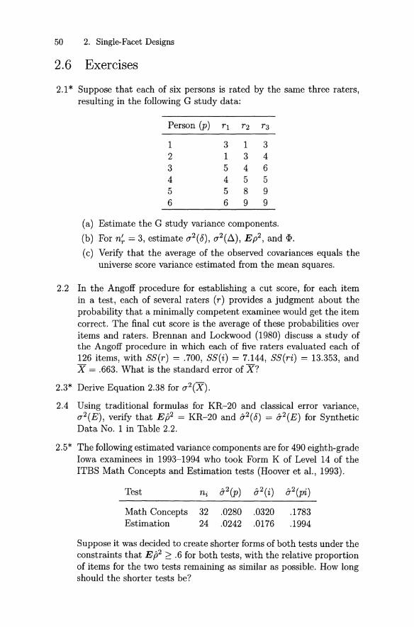
50 2. Single-Facet Designs

2.6 Exercises

2.1* Suppose that each of six persons is rated by the same three raters,resulting in the following G study data:

Person (p) rl

1 32 13 54 45 56 6

1 33 44 65 58 99 9

(a) Estimate the G study variance components.

(b) For n~ = 3, estimate 0'2(0), O'2(ß), E p2, and <1>.

(c) Verify that the average of the observed covariances equals theuniverse score variance estimated from the mean squares.

2.2 In the Angoff procedure for establishing a cut score, for each itemin a test , each of several raters (r) provides a judgment about theprobability that a minimally competent examinee would get the itemcorrect. The final cut score is the average of these probabilities overitems and raters. Brennan and Lockwood (1980) discuss a study ofthe Angoff procedure in which each of five raters evaluated each of126 items, with SS(r) = .700, SS(i) = 7.144, SS(ri) = 13.353, andX = .663. What is the standard error of X?

2.3* Derive Equation 2.38 for O'2(X) .

2.4 Using traditional formulas for KR-20 and classical error variance,O'2(E), verify that E{J2 = KR-20 and 0-2(0) = 0-2(E) for SyntheticData No. 1 in Table 2.2.

2.5* The following estimated variance components are for 490 eighth-gradeIowa examinees in 1993-1994 who took Form K of Level 14 of theITBS Math Concepts and Estimation tests (Hoover et al., 1993).

Test

Math ConceptsEstimation

32 .028024 .0242

.0320

.0176.1783.1994

Suppose it was decided to create shorter forms of both tests under theconstraints that E{J2 2: .6 for both tests, with the relative proportionof items for the two tests remaining as similar as possible . How longshould the shorter tests be?

2.6 Exercises 51

2.6 Verify that ~(A = X) = KR-21 = .725 for Synthetic Data Set No. 1,as reported in Table 2.12.

2.7* Consider the QUASAR data in Table 2.5. The average rating overpersons and tasks was 1.43, and recall that the tasks were scoredusing a five-point holistic scale (1 to 5). If an important decision werebased on an average rating of at least 3, how many tasks would berequired to have an error-tolerance ratio no larger than .5? (Do thecomputations with at least three decimal digits of accuracy.)

2.8 Prove that EMS(p) = (J2(pi) + ni (J2(p).

3Multifacet Universes of AdmissibleObservations and G Study Designs

Often, generalizability analyses may be viewed as two-stage processes. Thegoal of the first stage is to obtain estimated variance components for a Gstudy design, given a universe of admissible observations. The second stageinvolves using these estimated variance components in the context of a Dstudy design and universe of generalization to estimate quantities such asuniverse score variance, error variances, and coefficients. This dichotomy ofstages is somewhat arbitrary at times, but it is a conceptually meaningfuldistinction. Therefore, this chapter treats multifacet G study designs anduniverses of admissible observations, while Chapters 4 and 5 treat multi­facet D study design considerations and universes of generalization.

This chapter may be viewed as a treatment of analysis of variance thatis tailored to balanced designs in generalizability theory. A balanced designhas no missing data and, for any nested facet, the sampie size is constantfor each level of that facet . A notational system is described for charac­terizing G study designs and their effects. Also, algorithms, equations, andprocedures are provided for expressing mean scores in terms of score ef­fects (and vice versa), for calculating sums of squares, and for estimatingvariance components directly from mean squares . The algorithms and pro­cedures are very general and apply to practically any balanced design thatmight be encountered in generalizability theory, ranging from single-facetG study designs to very complicated multifacet ones. In the statisticallit­erature, the estimators of the variance components discussed here are thosefor the so-called "ANOVA procedure."

The topics in this chapter involve many conceptual, notational, and sta­tistical issues that are important in generalizability theory, as presented in

54 3. Multifacet G Study Designs

this book. However, some readers undoubtedly have prior familiarity withcertain topics (e.g., sums of squares in Section 3.3), and computer programssuch as GENOVA (see Appendix F) can be used to perform the numericalcomputat ions discussed here.

For the most part, issues are discussed from the perspective of two-facetuniverses and designs. This restriction is a convenience employed solely forillustrative purposes , rather than a limitation on generalizability theory orthe procedures , equations, and algorithms presented here.

3.1 Two-Facet Universes and Designs

Figure 3.1 provides Venn diagrams and model equations for some possibletwo-facet designs. Usually the two facets are associated with the indices iand h, and p represents the objects of measurement (often persons or exam­inees, but not always). In standard analysis of varian ce terminology, effectsin a design can be identified as either main effects or interact ion effects.From this perspective, p is associated with a main effect . For example, inthe p x i x h design, the main effects are lJp , lJi , and lJh , and all other effects(except J.L) are interaction effects . More simply, we can say that p, i, and hrepresent main effects and pi , ph, i h, and pih represent interact ion effects .For the two-facet designs in Figure 3.1, the effects are identified as follows.

Design Main Effects Interaction Effectsp x i x h p, i, h pi,ph, i h,pihp x(i :h) p,h,i :h ph, pi :h(i :p )x h p, h,i :p ph,ih:pi : (p x h) p, h, i: ph ph(i x h):p p, i :p, h:p ih:pi :h: p p, h:p,i :h:p

For each of these designs, other sources of residual error e are totally con­founded with the effect th at contains all three indices. From some perspec­tives, it is unusual to use the phrase "main effect" as a description of aneffect that involves nesting [e.g., the i:h effect in the p x (i :h) design], butin generalizability theory it is meaningful to associate each facet with amain effect.

Th ese notational convent ions, and the linear model representations ofthese designs, are considered in more detail in Section 3.2. Here, thesedesigns are first described from the perspective of Venn diagrams, and thenillustr ated in terms of some possible universes of admissible observations.

3.1.1 Venn Diagrams

In the Venn diagrams in Figure 3.1, each main effect is represented by acircle. Interaction effects are represented by the intersections of circles. The

3.1 Two-Facet Universes and Designs 55

total number of effects in any design is t he number of distinct areas in t heVenn diagram.

Wh en a main effect involves nesting, it is represented by a circle withinanother circle, or within the intersection of circles. For example, in t hep x (i :h) Venn diagram, the nested nature of t he i :h main effect is repre­sented by t he i circle being within t he h circle; and, in the i: (p x h) Venndiagram , t he nested nat ure of the i :ph main effect is represented by the icircle being within t he intersection of t he p and h circles.

3.1.2 Illustrative Designs and Universes

Für t he designs in Figure 3.1, the universe and popul ation sizes are denotedNi, Ni. , and N p. Unless ot herwise noted , it is assurned that t hey are infi­nite, or large enough to be considered so. The corresponding sampie sizesare denoted n i , nh , and n p ' Unless otherwise noted , it is assumed that con­ditions of i, h, and p are sampled at random. Note that t he ind ices p, i , andh do not designate any partic ular facets , groups of condit ions, or objectsof measurement . Specifically, i does not necessarily represent items, and pdoes not necessarily represent persons.

Next, examples of each of t he illust rative designs are briefly described,given cert ain universes of admissible observations. In these examples, someissues are introduced (without much explanation) to motivate discussionof related topics in subsequent sections of this and later chapt ers.

Items-Crossed-with-Raters in the Universe of Admissibleobservations

Suppose t hat it ems (i) are crossed wit h raters (r) in t he universe of ad­missible observat ions. T his means t hat any one of the N i items might berated by any one of t he N; raters. If the populat ion is crossed wit h t hisuniverse of admissible observat ions, then t he corresponding G study designis p x i x r , in which the responses of n p persons to ni items are each eval­uated by nr rat ers. Esti mated variance components for this fully crosseddesign can be used to est imate results for any possible two-facet design.However , for t he i x r universe, an investigator might conduct a G st udyusing any one of the ot her two-facet designs.

Suppose, for example, t hat n p persons are administe red n i = 12 items,and each of nr = 3 raters evaluates nonoverlapping sets of four items each.This a verb al descript ion of t he p x (i :r) design with n i = 4. It is an ent irelylegiti mate G st udy design for t he universe of admissible observatio ns t hathas i x r. T hat is, even though the universe of admissible observations hascrossed facets, the G st udy design may have nested facets . An investigatorpays a price, however , for using the p x (i: r) design (or any design ot herthan p x i x r ) when t he universe of admissible observat ions is crossed­namely, t he est imated variance components from t he p x (i :r ) design can

56 3. Multifacet G Study Designs

p x i x h Design

J-t Xpih J-t

+(J-tP-J-t) +lIp

+(J-ti-J-t) +lIi

+(J-th-J-t) +lIh

+ (J-tpi - J-tp - J-ti + J-t) + IIpi

+ (J-tph - J-tp - J-th + J-t) + Vph.

+ (J-tih - J-ti - J-th + J-t) + lIih

+ (Xpih - J-tpi - J-tph - J-tih + IIpih

J-tp + J-ti + J-th - J-t)

p

p x (i: h) Design

J-t Xpih

+ (J-tp - J-t)

+ (J-th - J-t)

+ (J-tih - J-th)

+ (JLph - JLp - JLh + JL)

+ (Xpih - J-tph - J-tih + J-th)

J-t

+ IIp

+ IIh

+ lIi:h

+lIph

+ IIpi:h

(i:p) x h Design

h

J-t Xpih

+ (J-tp - J-t)

+ (J-th - J-t)

+ (J-tip - J-tp)

+ (J-tph - J-tp - J-th + J-t)

+ (Xpih - J-tph - J-tip + J-tp)

J-t

+ IIp

+ IIh

+ lIi:p

+ IIph

+ lIih:p

FIGURE 3.1. Venn diagrams and linear models for some two-facet designs .

3.1 Two-Facet Universes and Designs 57

p

JL Xpih

+ (JLp - JL )

+ (JLh - JL )

+ (JLph - JLp - JLh + JL )

+ (Xpih - JLph )

JL

+ vp

+ vh+Vph

+ Vi:ph

i : (p x h) Design

(i x h) :p Design

JL Xpih

+ (JLp - JL )

+ (JLi p - JLp)

+ (JLhp - JLp )

+ (Xpih - JLip - JLhp + JLp )

JL

+vp

+Vi:p

+ vh :p

+ Vih:p

i : h :p Design

Xpih JL Xpih

+ (JLp - JL )

+ (JLhp - JLp )

+ (Xpih - JLhp)

= JL

+vp

+Vh:p

+ Vi:h:p

FIGURE 3.1 (cont inued). Venn diagrams and linear models for some two­facet designs.

58 3. Multifacet G Study Designs

be used to estimate results for only some two-facet D studies. On the otherhand, the p x (i: r) design has a distinct advantage if rater time is at apremium.

Clearly, then, there is no universal answer to the question, "What Gstudy design should be used?" The investigator must make this decisiontaking into account the nature of the universe of admissible observations,likely D study considerations (not yet specified in detail), and time and costconsiderations. All things considered, however, it is generally preferablethat the sample sizes for a G study design be as large as possible. Doing sohelps ensure that the resulting estimated variance components will be asstable as possible.

As another example of a G study design given an i x r universe of admis­sible observations, suppose each person is administered a different sampieof ni items, but all items are evaluated by the same set of nr raters. This is averbal description of the (i: p) x r design. It has the advantage of samplinga total of npni items, rather than only ni items, but, again, the resultingestimated variance components cannot be used to estimate results for allpossible two-facet D study designs.

Iterns-Crossed-with-Occasions in the Universe of AdmissibleObservations

Suppose that items (i) are crossed with occasions (0) in the universe of ad­missible observations. The structure of this universe and the one discussedabove (i x r) are the same, but one of the facets is different. If the popula­tion is crossed with the i x 0 universe of admissible observations, then thecorresponding G study design is p x i x 0 , in which each person respondsto a set of ni items, all of which are administered on no different occasions.Again, however, G study data might be collected using any one of the othertwo-facet designs.

For example, suppose that (a) each person responds to a set of ni itemsadministered on no occasions; (b) for each person , the occasions or times ofadministration are the same; and (c) for each person and each occasion, theni items are different. This is a verbal description of the i: (p x 0) design.In conventional ANOVA terminology, this is the frequently discussed ran­dom effects two-way factorial design with replications (items) within cells.However, this ANOVA description is a potentially misleading way to char­acterize the i: (p x 0) design in generalizability theory, because the i facetdoes not play the role of within-cell replications in the traditional ANOVAsense. Indeed, many designs frequently encountered in generalizability the­ory can be given a conventional ANOVA verbal description, or somethingelose to it, but doing so can cause confusion about the nature and role offacets in generalizability theory. For this reason, such conventional ANOVAdescriptions of designs are rarely used here.

3.1 Two-Facet Universes and Designs 59

As another example of a G st udy design for the i x 0 universe of admis­sible observations, suppose that : (a) each person is administe red a set ofni items on n o occasions; (b) for an individual person the same items areadministe red on each occas ion; but (c) for different persons t he items aredifferent and t he occasions are different. This is a verbal descriptio n of t he(i x 0) :p design.

Also, t he design could be i :o: p. For t his design, (a) each person is admin­istered different items on different occasions, and (b) for different personst he occasions (of t est administ rat ion) are different. This design is some­times called the fully nested design. As such, it is the two-facet analogueof t he i :p design discussed in Chapte r 2.

Items-Nested-Within-Content Categories in the Universe ofAdmissible Observations

Universes of admissible observat ions do not always have all facets crossed .For example, many tests are best viewed as being made up of items (i)nested within conte nt categories (h). In such cases, it is frequentl y reason­able to view the universe of admissible observations as i :h, with every itemin t he universe being associated with one and only one conte nt category h.In addit ion, the numb er of content categories N h is usually quite small.

For an i :h universe of admissible observations of the type describedabove, a G st udy p x i x h design is a logical impossibility. This designwould be reasonable only if every item could be associated with everyconte nt category in the universe, which directly contradicts t he previousdescription of t he universe of admissible observations. There is frequentlyan addit ional issue involved in using this design with a nested universe ofadmissible observat ions; namely, all Nh conte nt categories are usually rep­resented in t he design specifications, implying t hat nh = Nh < 00 . Underthese circumstances, t he model is described as mixed , rather t han random,and the est imated vari ance components are associated with a fixed facet h,with a finite universe of N h condit ions.

When the universe of admissible observat ions has i:h, any G study designmust also have i:h. Ofthe designs in Figure 3.1 only two designs, other thanp x (i :h) , have this characte rist ic. They are the i: (p X h) and i:h:p designs.However , when nh = Ni, < 00, the i :h:p design is not a likely possibilitybecause it necessitates independent samples of content categories for eachperson. For the i: (p x h) design, each person is administe red a differentsam ple of items for each of the n h = Nh content categories.

Persons as a Facet in the Universe of Admissible Observations

Usually persons are viewed as t he objects of measurement , but the t heoryper se does not dictate that persons play this role. Suppose t hat D st udyconsiderations ultim ately will focus on d ass means as t he objects of mea­surement . (For exa mple, t he reliability of d ass means is somet imes a topic

60 3. Multifacet G Study Designs

of concern in program evaluation contexts.) In such cases, the universe ofadmissible observations may have persons crossed with items .

For such a universe of admissible observations, a design often consideredis (p: c) x i, where p, c, and i stand for persons, classes, and items, re­spectively. This (p:c) x i design is simply a specific instance of the generic(i :p) x h design in Figure 3.1. Again, the p, i, and h indices used in spec­ifying the generic two-facet designs do not necessarily stand for persons,items, and some other facet, respectively.

Any group of conditions (persons, items, raters, occasions, classes, etc .)could be considered the objects of measurement. However, strictly speaking,the specification of objects of measurement is a D study consideration.Therefore, further discussion is postponed until Chapter 4.

Other Universes of Admissible Observations and G StudyDesigns

The foregoing discussion illustrates only a very small number of possibleuniverses of admissible observations, G study designs, and related issues.For example, there are other possible two-facet designs, and the number ofpossible designs increases exponentially as the number of facets increases.Also, in theory, the number of possible facets in a universe of admissibleobservations is unlimited, although practical constraints usually precludeusing large numbers of facets in any particular G study.

Furthermore, designs associated with nested universes are sometimes un­balanced (e.g., unequal numbers of items in content categories) and some­times best approached by means of multivariate generalizability theory.Such complexities are treated in later chapters.

The algorithms and procedures discussed next are relevant for a verylarge class of balanced, univariate G study designs, no matter how manyfacets are involved. However, for illustrative purposes, only the p x i x hand p x (i :h) designs are used extensively in the following sections of thischapter.

3.2 Linear Models, Score Effects, and Mean Scores

Figure 3.1 contains two expressions for the linear models associated witheach of the two-facet designs introduced in Section 3.1. The first expressionprovides a decomposition of an observable score Xpih in terms of meanscores, while the second expression provides the decomposition in terms ofscore effects. The two expressions are simply different ways of expressingthe same decomposition, which is a tautology. In this section, a notationalsystem, algorithm, and equations are presented for expressing, relating, andinterpreting effects in linear models.

3.2 Linear Models, ScoreEffects, and Mean Scores 61

The algebraic expressions for the models in Figure 3.1 do not, in and ofthemselves, provide a sufficient basis for analyzing G study data, however.An investigator must also specify the nature of any sampling involved.Except for Section 3.5, it is assumed in this chapter that n < N --; 00

for each facet (as weIl as the objects of measurement "facet"), and thatall sampling is random. When these assumptions are applied to equationssuch as those in Figure 3.1, the resulting models are referred to as randomeffects linear models.

3.2.1 Notational System for Main and Interaction Effects

In the notational system used here, any main effect can be represented inthe following manner:

{primary } { first nesting } {second nesting}index . index (indices) . index (indices) " ..

Main effects that involve nesting are sometimes referred to as nestedmain effects, and those that do not involve nesting are sometimes callednonnested main effects. If a main effect does not involve nesting, then it isrepresented by the primary effect index only. Note that a nesting index fora specific main effect is usually a primary index for some other main effect.For example, in the p x (i: h) design the index h is a nesting index in thenested main effect i:h, and h by itself is also a nonnested main effect.

For the illustrative designs in Figure 3.1 no main effect involves a "sec­ond" nesting index . However, more complicated designs do sometimes in­volve two and even three levels of nesting. It is for this reason that thenotation for a main effect has been specified very generally. Some otherauthors denot e a nested main effect by placing all nesting indices withinparentheses, no matter what level of nesting is involved. For example , if adesign involves the main effect a:b:c, some authors denote it a(bc). Herethe notation a:b:c is preferred because it directly implies that levels of aare nested within levels of b which are nested within levels of c, whereasa(bc) could mean that levels of aare nested within all combinations of alevel of b with a level of c.

Each inter action effect can be represented as a combination of maineffects in the following manner.

{

combination Of} {COmbination Of} {COmbination of }primary : first nesting : second nesting : . . .

index (indices) index (indices) index (indices)

The entire set of interaction effects is obtained by forming all valid combi­nations of main effects. Any such combination is valid provided no indexappears as both a primary and a nesting index. Also, if an index appears

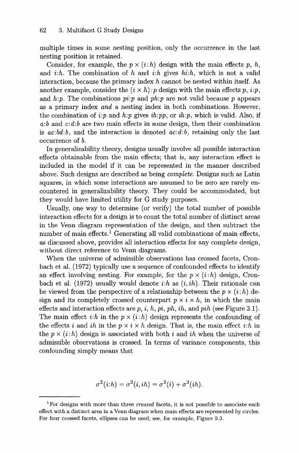
62 3. Multifacet G Study Designs

multiple times in some nesting position, only the occurrence in the lastnesting position is retained.

Consider , for example, the p x (i :h) design with the main effects p, h,and i :h. The combination of hand i:h gives hi :h, which is not a validinteraction, because the primary index h cannot be nested within itself. Asanother example, consider the (i x h) :p design with the main effects p, i :p,and h:p. The combinations pi :p and ph:p are not valid because pappearsas a primary index and a nesting index in both combinations. However,the combination of i:p and h:p gives ih :pp, or ih:p, which is valid. Also, ifa:b and c:d:b are two main effects in some design, then their combinationis ac:bd:b, and the interaction is denoted ac:d:b, ret aining only the lastoccurrence of b.

In generalizability theory, designs usually involve all possible interactioneffects obtainable from the main effects; that is, any interaction effect isincluded in the model if it can be represented in the manner describedabove. Such designs are described as being complete. Designs such as Latinsquares, in which some interactions are assumed to be zero are rarely en­countered in generalizability theory. They could be accommodated, butthey would have limited utility for G study purposes .

Usually, one way to determine (or verify) the total number of possibleinteraction effects for a design is to count the total number of distinct areasin the Venn diagram representation of the design, and then subtract thenumber of main effects.! Generating all valid combinations of main effects,as discussed above, provides aB interaction effects for any complete design,without direct reference to Venn diagrams.

When the universe of admissible observations has crossed facets , Cron­bach et al. (1972) typically use a sequence of confounded effects to identifyan effect involving nesting. For example , for the p x (i :h) design, Cron­bach et al. (1972) usually would denotei :h as (i, ih) . Their rationale canbe viewed from the perspective of a relationship between the p x (i :h) de­sign and its completely crossed counterpart p x i x h, in which the maineffects and interaction effects are p, i, h, pi , ph, ih, and pih (see Figure 3.1).The main effect i:h in the p x (i :h) design represents the confounding ofthe effects i and ih in the p x i x h design. That is, the main effect i :h inthe p x (i :h) design is associated with both i and ih when the universe ofadmissib le observations is crossed. In terms of variance components, thisconfounding simply means that

1 For designs with more than three crossed facets, it is not possible to associate eacheffect with a distinct area in a Venn diagram when main effects are represented by circles.For four crossed facets , ellipses can be used ; see, for example, Figure 9.3.

3.2 Linear Models, Score Effects, and Mean Scores 63

Similarly, pi :h represents the confounding of pi and pih.2

Using the not ation introduced above, it is relatively simple to determinewhich effects from a fully crossed design are confounded in an effect for adesign that involves nesting; namely,

Confounded-Effects Rule: The effects that are confounded are allthose th at involve only indices in the nested effect and that includethe primary index (indices) in the nested effect .

The number of effects th at are confounded in a nested effect is

2 Exp(number of nesting indices),

where Exp means "exponent ial" or "raised to the power." For example,for the effect i:h:p, there are 2 Exp(2) = 4 confounded effects (i, ih, ip,and i hp) when the universe of admissible observat ions has i x h , and p iscrossed with both facets. A notational shorthand for thi s result is:

i :h:p =? i, ih, ip, ihp.

In this book, the operator ":" is used to represent nested effects, becauselisting the sequence of confounded effects is notationally burdensome, es­pecially for complicated designs. Even so, underst anding the confoundedeffects not ation is important, because confounded effects relat e directly tothe universe of admissible observations. By cont rast, the nested effects no­tation relates most directly to the G study design.

Note, however , th at a thou ghtless translat ion of the nested effects nota­tion to the confounded effects notation can lead to nonsensical results . Forexample, with a nested universe of admissible observat ions, such as i :h , itis meaningless to represent th e main effect i:h as (i , ih) , because i and i hare not distinguishable in the universe of admissible observations.

3.2.2 Linear Models

Given these notational convent ions, the linear model for a design can berepresented, in general, as

(3.1)

where

w all indices in the design,

J-L grand mean,

2T his does not rnean t hat variance cornpo nents should be esti rnated for a crosseddesign when the design actually involves nesting.

64 3. Multifacet G Study Designs

a = the index (indices), with any nesting operators,

for any component in the design,

Ver score effect associated with e, and

I: Ver sum of all score effects (except J.L) in

the design under consideration.

Equation 3.1 provides a decomposition of the observed scores X w in termsof score effects Ver' For example, in the p x (i: h) design, w is simply pih,and Ver is used generically to represent score effects associated with thecomponents p, h, i:h, ph, or pi:h.

For the designs in Figure 3.1, the linear models resulting from specificapplications of Equation 3.1 are provided to the far right of the Venn dia­grams. These equations are the most concise and convenient ways to rep­resent the linear models. However, from the perspective of generalizabilitytheory, the linear model expressions immediately to the right of the Venndiagrams are more fundamental, because score effects are always definedin terms of mean scores in generalizability theory. To obtain these meanscore decompositions of X w , an investigator needs to be able to expressany score effect Ver in terms of a linear combination of mean scores. Analgorithm for doing so is provided later, but first we consider definitions ofmean scores for the universe and population, and assumptions for randomeffects models.

In random effects linear models, it is assumed that N -4 00 for all facetsincluding the object of measurement "facet ." For the populations and uni­verses in Figure 3.1, this means that Np -4 00, Ni -4 00, and Nh -4 00.

Under these circumstances, the grand mean in the population and universeis defined as

(3.2)

where w is the set of all indices in the design. Also, the universe (or popu­lation) mean score for any component o is defined as

(3.3)

where ci (note the dot over a) is the set of all indices in w that are notcontained in a . For example, in the p x (i: h) design,

J.Lh

J.Lih

= EEEXpih,p i h

= E ~ Xpih, andp t

EXpih.p

When the design is p x (i: h), there is a potential source of confusionin denoting Ep(Xpih) as J.Lih, rather than J.L i:h' This potential confusion

3.2 Linear Models, Score Effects , and Mean Scores 65

arises because the score effect (for the design) associated with this meanscore (for the universe) is Vi .tv- Unless a specific context dictates otherwise,in this book mean scores for the population and universe are representednotation ally with respect to a crossed universe of admissible observat ionswhich, in turn, is crossed with the population, whereas score effects aredenoted in terms of the act ual design employed. For example, even if thedesign is p x (i :h), when the population and universe consist of crossedfacets , i is not nested within h in the universe and, therefore, JLih (ratherth an JL i :h) correctly reflects the st ructure of the universe. However, if theuniverse of admissibl e observations had i nested within h, then JL i :h wouldbe more descriptive. These notational considerations with respect to meanscores highlight the fact th at , in a specific context, a G study design shouldbe viewed in conjunction with a specified population and universe of ad­missible observations.i'

The definitions of mean scores in Equations 3.2 and 3.3, and the mannerin which score effects are defined, imply that the expected value of anyscore effect V« (for any index in 0: ) is zero:

EVa = O. (3.4)

(3.5)

If this were not so, then th e linear models in Figure 3.1 would not betautologies.

Now, given Equations 3.2 through 3.4, it follows th at one can expressthe mean score for any component 0: in terms of score effects as

{sum of score effects for all components that

JL a = JL + consist solely of one or more indices in 0:.

For example, in the p x (i: h) design,

JL ih = JL + Vh. + Vi :h , (3.6)

which can be verified by replacing X pi h in Equation 3.3 with its decompo­sition in terms of score effects:

JLih E Xpihp

E(JL + v p + Vh + Vi :h + Vph. + Vpi :h)p

JL + E Vp + Vh + vi:h + E Vph + E Vp i .h »p p p

The result in Equation 3.6 follows immediately upon recognizing that Epvp ,

EpVph , and EpVpi :h are all zero, because the expected value of an effect overany of its subscripts is zero.

3In t his bo ok, an obs erved score for single conditions in the un iverse of admissibleobservat ions and/or t he G st udy is not denoted using t he nest ing operator. So, even ift he design is p X (i :h) , the observed score is denoted X pih , not X pi:h.

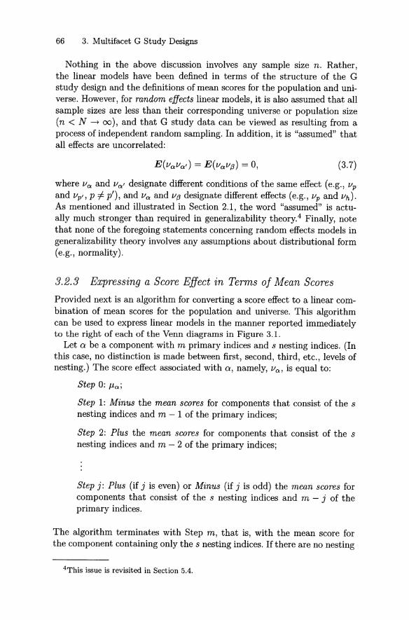
66 3. Multifacet G Study Designs

Nothing in the above discussion involves any sample size n. Rather ,the linear models have been defined in terms of t he st ruct ure of the Gstudy design and the definitions of mean scores for the population and uni­verse. However, for random effects linear models, it is also assumed that allsample sizes are less th an their corresponding universe or population size(n < N --+ (0), and that G study data can be viewed as resultin g from aprocess of indep endent random sampling. In addition, it is "assumed" thatall effects are uncorrelated:

(3.7)

where Va: and Va:' designate different condit ions of the same effect (e.g., vp

and vp' , p f p') , and V« and vß designate different effects (e.g., vp and Vh).

As mentioned and illustrated in Section 2.1, the word "assumed" is actu­ally much stronger th an required in generalizability theory." Finally, notethat none of the foregoing statements concerning rand om effects models ingeneralizability theory involves any assumpt ions about distributional form(e.g., normality).

3.2.3 Expressing a Score Effect in Terms 0/ Mean Scores

Provided next is an algorithm for converting a score effect to a linear com­bination of mean scores for the population and universe. This algorit hmcan be used to express linear models in the manner reported immediatelyto the right of each of the Venn diagrams in Figure 3.1.

Let a be a component with m primary indices and s nest ing indices. (Inthis case, no dist inction is made between first , second, third , etc ., levels ofnesting.) The score effect associated with o, namely, Va: , is equal to :

Step 0: Jla: ;

St ep 1: Minus the mean scores for components th at consist of the snesting indices and m - 1 of the primary indices;

St ep 2: Plus the mean scores for components th at consist of the snesting indices and m - 2 of the primary indices;

St ep j : Plus (if j is even) or Minus (if j is odd) the m ean scores forcomponents that consist of the s nesting indices and m - j of theprimary indices.

The algorithm termin ates with Step m, that is, with the mean score forthe component containing only the s nesting indices. If there are no nestin g

4This issue is revisit ed in Section 5.4.

3.3 Typical ANOVA Computations 67

indices in the component 0:, then Step m results in adding or subtractingJ..l.

Consider, for example, the component pi :h in the p x (i:h) design. Thiscomponent has a single nesting index h, and two primary indices p andi. Step 1 in the algorithm results in subtracting J..lph and J..lih from J..lpih,

because both J..lph and J..lih involve the nesting index hand 2 - 1 = 1 of theprimary indices in pih. Step 2 results in adding J..lh to the result of Step 1because J..lh is the mean score that involves the nesting index hand 2- 2 = 0of the primary indices in pi :h. Therefore,

Vpi:h = J..lpih - J..lph - J..lih + J..lh ·

In the p x (i :h) design with one observation per cell, J..lpih is indistinguish­able from Xpih and, therefore, we usually specify Vpi.h. as

Vpi:h = X pi h - J..lph - J..lih + J..lh·

This latter representation of Vpi:h rather clearly indicates the "residual"nature of this effect in the p x (i :h) design.

3.3 Typical ANOVA Computations

This section provides a treatment of observed mean scores, score effects,sums of squares, degrees of freedom, and mean squares for complete bal­anced designs. Readers familiar with these topics might skim this section,paying attention primarily to notational conventions.

3.3.1 Observed Mean Scores and Score Effects

For each component 0:, the mean score J..lo: has an observed score analogue,denoted X 0:, which is

- 1 ""x; = -(.) 6Xw'7l' 0: .

0:

(3.8)

(3.9)

As in Equation 3.3, a (note the dot above 0:) refers to the set of indices inw that are not included in 0: . For any index in a, the summation runs from1 to the sampie size (n) associated with the index, and

. {I if 0: = Wi and , otherwise, the product7l'(0:) = of the sampie sizes for all indices in o.

Consider, for example, the i component in the p x i x h design. Theobserved mean score associated with a particular item is

68 3. Multifacet G Study Designs

Similarly, for the pi component,

_ 1 nh

x ; = - L:Xpih.nh h=l

For the notational system used here, when a mean is taken over the levelsof a facet, the index for that facet does not appear in the subscript for themean score. Given this convention, it follows from Equation 3.8 that theestimate of the grand mean (i.e., the observed score analogue of J.L) is

(3.10)

where 1f(w) is the product of the sample sizes for all indices in the design.For example, in the p x i x h design,

In summary, then, we use X 0 to denote the observed score analogue ofJ.Lo, and we use X to denote the observed score analogue of J.L. Also, weuse Xo to denote the observed score analogue of vo .5 Equations 3.1, 3.5,and the algorithm in Section 3.2.3 are applicable to the observed scoreanalogues of J.Lo and vo' One simply replaces J.Lo, vo, and J.L with Xo, xo,and X , respectively. For example, in terms of observed mean scores for thep x i x h design,

Xpih = X + xp + Xi + Xh + Xpi + Xph + Xih + Xpih,

and application of the algorithm to the X o terms in this equation gives

Xpih = X+(Xp-X)+(Xi-X)+(Xh- X)

+ (X pi - X p - Xi + X) + (Xph - X p - X h + X)

+ (Xih - Xi - Xh + X)

+ (Xpih - X pi - Xph - Xih + X p + X, + X h - X) .

This familiar decomposition of Xpih in terms of observed mean scores isclearly analogous to the linear model decomposition in terms of J.Lo meanscores in Figure 3.1.

5This is reasonably consistent with other literature in which observed deviation scoresare identified with lowercase roman letters, although Brennan (1992a) uses X", rw,

3.3 Typical ANOVA Computations 69

3.3.2 Sums 0/Squares and Mean Squares

Given these not ational conventions, the sum of squares for any componenta in any design is

SS(a) = 7l"(Ö:)LX~ ' (3.11)

where the summation is taken over all indices in o . Also, t he total sum ofsquares is

(3.12)w

where the summation is taken over all indices in the design.For example, for the p x i x h design, the sum of squares for the i com­

ponent isn i n i

SS(i) = npnhLX~ = npnh L(Xi - X) 2,i = l i=l

the sum of squares for the pi component is

SS(pi ) = nh L LX~i = nh L L(Xpi - X p - x, + X)2 ,p p

and the total sum of squares is

SS(tot ) = LLL(Xpih - X) 2.p h

(3.13)

(3.14)

(3.15)

The definition of SS(a ) in Equat ion 3.11 can be used directly to obt ainthe sum of squares for any component in any complete balanced design.The process of doing so tends to be tedious, however. A simpler procedureis discussed next .

For the component o, let the "sum of squared mean scores" be

(3.16)

where the summation is taken over all the indices in o . An equivalentexpression in terms of squared total scores is

where the summation in parentheses is taken over all indices in w t hat arenot in o .

Note the distinction between SS(a) in Equation 3.11 which involves x'"terms, and T (a) in Equation 3.16 which involves X ", terms. A special caseof Equ ation 3.16 is

- 2T( J1.) = 7l" (w)X , (3.17)

70 3. Multifacet G Study Designs

which is the "sum of squared mean scores" associated with the grand mean.Expressing sums of squares with respect to T terms is st raight forward­

use the algorithm in Section 3.2.3 with V« , /La, and /L replaced by SS(a) ,T(a), and T(/L), respectively. For example , in the p x i x h design, ratherthan using Equation 3.13 to calculate SS(i) , a computat ionally simplerexpression is

SS(i) = T(i ) - T (/L).

Similarly,SS(pi) = T(pi ) - T(p) - T(i ) + T (/L)

can be used instead of Equation 3.14, and

SS(tot) = T(pih) - T(/L)

is more efficient computationally than Equation 3.15.Appendix A provides formulas for T(a) and SS(a) for each component

in each of the illustrative designs in Figure 3.1. These tables also provideformulas for degrees of freedom df (a). For an effect (main effect or inter­action ) that is not nested, the degrees of freedom are the product of the(n - l )s for the indices in the effect, where n is the G st udy sample sizeassociated with the index. For any nested effect, t he degrees of freedom are

{product of (n - l )s } { product of ns }for primary indices x for nesting indices .

Mean square s are simply

SS(a)MS(a) = df(a) ' (3.18)

3.3.3 Synthetic Data Examples

Table 3.1 provides Synthetic Data Set No. 3, with sample means, for thep x i x 0 design with np = 10 persons, ni = 4 items, and no = 2 occasions.Assurne that the infinite universe of admissible observations has i x 0 , andthe data in Table 3.1 arose from a process of independent random samplingfrom this universe .

Clearly, this data set is not an example of an ideal G study, especiallysince the sample sizes are so small. However, the small sample sizes makeit relat ively easy to verify the usual ANOVA statist ics in Table 3.3. Forexample, using Equation 3.16,

4

T( ,; ) ~x2• npn o 6 i

i=l

= (10)(2)[(4.10)2 + (5.56) 2 + (5.80)2 + (5.56)2]

2263.50,

3.3 Typical ANOVA Computations 71

and using Equation 3.17

Therefore,

SS(i) = T( i) - T(f.L) = 2263.50 - 2226.05 = 37.45.

Table 3.2 provides Synthet ic Dat a Set No. 4, with sample means, for thep x (r: t) design with np = 10 persons and nt = 3 tasks, and with each taskevaluated by a different set of n r = 4 raters. Even though raters are nestedwithin tasks in the G study design, suppose raters are crossed with tasksin the universe of admissible observations. This assumption has no bearingon the computations of sums of squares, but it does affect the manner inwhich the sampling presumably occurred. Th at is, raters and tasks wereboth sampled independently, and nr = 4 raters were randomly assigned toeach of the nt = 3 tasks.

The usual ANOVA statistics for Synthetic Dat a Set No. 4 are providedin Table 3.4. For example,

T(pt) n r LLX~tp t

4[(5.25)2 + (4.25)2 + ... + (3.50)2]

2931.5000,

T(p) nr nt L X~p

(4)(3)[(4.75)2 + (5.75)2 + ...+ (4.00) 2]

2800.1667,

T(t) npnr L X~t

(10)(4)[(5.50)2 + (4.80)2 + (3.95)2]

2755.7000,

and

Therefore,

SS(pt) T(pt) - T(p) - T(t) + T(f.L)

= 2931.5000 - 2800.1667 - 2755.7000+ 2707.5000

83.1333.

-.:l

l'-J w

TA

BL

E3.

1.S

ynth

etic

Dat

aS

etN

o.

3an

dth

ep

xi

x0

Des

ign

~

x.:

S e-e

x.;

Xp

o~

01

02o <1

le-e

-

Per

son

ili2

i3i4

i 1i2

i3i4

i 1i2

i3i4

010

2X

p0 tr

:1

26

75

25

55

2.0

5.5

6.0

5.0

5.00

4.2

54

.625

e-t- .:: 0-

24

56

76

75

75.

06.

05.

57.

05

.50

6.25

5.87

5'< t:J <1

l

35

54

65

45

55.

04.

54.

55.

55.

004

.75

4.8

75U

l aq'

::l4

59

86

57

76

5.0

8.0

7.5

6.0

7.00

6.25

6.62

5U

l

54

35

64

56

44.

04.

05.

55

.04.

504.

754

.625

64

44

76

47

85

.04

.05

.57.

54.

756.

255

.500

72

66

52

77

52.

06.

56.

55

.04.

755.

255.

000

83

44

56

66

44.

55.

05.

04

.54

.00

5.50

4.7

50

90

54

55

55

32.

55.

04

.54

.03.

504

.50

4.00

0

106

87

66

88

66.

08

.07.

56.

06.

757.

006.

875

Xio

for

0=

1X

iofo

r0

=2

Xi

Xo

X

3.5

5.5

5.5

5.8

4.7

5.8

6.1

5.3

4.10

5.65

5.80

5.55

5.0

755.

475

5.27

5

TA

BL

E3.

2.S

ynth

etic

Dat

aS

etN

o.4

and

the

px

(r:t

)D

esig

n

Xp

rt

tlt2

t3x.

;P

erso

nT

lT

2T

3T

4T

ST

6T

7T

8T

gT

lOT

UT

l2t

lt2

t3X

p

15

65

55

34

56

73

35.

254.

254.

754.

750

29

37

77

55

57

75

26.

505.

505.

255.

750

33

43

35

33

56

51

63.

254

.00

4.50

3.9

17

47

55

33

14

35

33

55.

002.

754.

003.

917

c...o~

59

29

77

73

72

75

36.

756.

004.

255.

667

~6

34

35

33

63

45

12

3.75

3.75

3.00

3.50

0"0 ;:;

.

77

55

75

55

46.

006.

004.

755.

583

E.

77

37

>8

58

57

75

54

32

11

6.25

5.25

1.75

4.4

17Z 0

99

98

86

66

55

81

18

.50

5.75

3.75

6.00

0~ 0

104

44

33

56

55

71

13

.75

4.75

3.50

4.00

00 3

Xr

: tfü

rt

=1

Xr

: tfü

rt

=2

Xr

: tfü

rt

=3

Xt

X"0 I:: ~ \ll e-e

-

6.1

4.8

5.6

5.5

5.3

4.3

4.7

4.9

4.8

5.6

2.6

2.8

5.5

04.

803.

954

.750

ö' :l CIl

~ c...o

74 3. Multifacet G Study Designs

TABLE 3.3. ANOVA fOT P x i x 0 Design Using Synthetic Data Set No. 3

Effect(a) df(a) 1f(a) T(a) SS(a) MS(a) a-2 (a )

p 9 8 2288.25 62.20 6.9111 .5528

3 20 2263.50 37.45 12.4833 .4417

0 1 40 2229.25 3.20 3.2000 .0074

pi 27 2 2382.00 56.30 2.0852 .5750

po 9 4 2303.50 12.05 1.3389 .1009

io 3 10 2274.20 7.50 2.5000 .1565

pio 27 1 2430.00 25.25 .9352 .9352

Mean(J1.) 80 2226.05

Total 79 203.95

TABLE 3.4. ANOVA for p x (r: t) Design Using Synthetic Data Set No. 4

Effect (a ) df(a ) 1f(a) T(a) SS(a) MS(a) a-2 ( o)

p 9 12 2800.1667 92.6667 10.2963 .4731

t 2 40 2755.7000 48.2000 24.1000 .3252

r.t 9 10 2835.4000 79.7000 8.8556 .6475

pt 18 4 2931.5000 83.1333 4.6185 .5596

pr:t 81 1 3204.0000 192.8000 2.3802 2.3802

Mean(J1.) 120 2707.5000

Total 119 496.5000

3.4 Random Effects Variance Components

This section treats definitions and interpretations of G study random effectsvariance components, procedures for expressing expected mean squares inte rms of t hese variance components, procedures for estimating random ef­fects variance components, and some other issues associated with G studyrandom effects variance components. To avoid ot herwise awkward verbaldescriptions, in this sect ion t he word "facet" is used to refer to eit her afacet in t he universe of adm issible observat ions or the "facet" associatedwith t he objects of measureme nt.

3.4. 1 Defining and Interpreting Variance Components

There is a variance component associated with each of the score effects inthe linear model equation for any G study design. In general , for a randomeffects model , the variance component for a is

(3.19)

(3.20)

3.4 Random Effects Variance Components 75

and it is called a random effects variance component. In words, (i2(0:) isthe variance , in the population and/or universe, of the score effects VQ; or,the expected value of the square of the VQ' For example, for the p x (i: h)design,

The last result in Equation 3.20 results from expressing Vh in terms of meanscores for the universe of admissible observations and the population. Also,since J-L is a constant in Equation 3.20,

Evidently, (i2(h) may be interpreted either as the variance of the h-facetscore effects, or as the variance of the h-facet mean scores. Indeed, whenever0: is a nonnested main effect (i.e., 0: consists of a single index),

When 0: is an interaction effect or a nested main effect,

For example, in the p x (i :h) design,

(i2(ph) = (i2(Vph) = E V;h = E(J-Lph - J-Lp - J-Lh + J-L)2,

which is not (i2(J-Lph) ' Another way to express (i2(ph) is

E[(J-Lph - J-L) - (J-Lp - J-L) - (J-Lh - J-L)f

E[(J-Lph - J-L) - Vp - vhf ·

That is, (i2(ph) can be viewed as the expected value of the square of(J-Lph - J-L) after removing the effects of p and h.

As another example , consider the variance component for the nestedmain effect i :h in the p x (i :h) design:

(3.21)

Now, if i x hin the universe of admissible observations, then Equation 3.21can be expressed in terms of universe mean scores as:

That is, (i2(i :h) is interpretable as the expected value ofthe squared devi­ation mean scores of the form J-Lih - J-Lh . Alternatively, if i :h in the universeof admissible observations, then Equation 3.21 can be expressed as

76 3. Multifacet G Study Designs

using the nesting operator in J.Li :h to explicitly reflect the nesting in theuniverse. In words, when the universe of admissible observations has i:h,then a2(i :h) is interpretable as the expected value, over the h facet , ofthevariance of the i-facet mean scores within a level of h.

In interpreting G study variance components, it is also helpful to viewthem as providing a decomposition of total variance. Specifically,

(3.22)

where the summation is taken over all components in the design . For ex­ample, for the p x (i: h) design the total variance is

a2(Xpi h ) = a2(p) + a2(h) + a2(i :h) + a2(ph) + a2(pi :h).

Equation 3.22 indicates that any a2(a) represents that part of a2 (X w ) thatis uniquely attributable to the component o. Furthermore, since X w is theobserved score associated with a single condition of each facet, the variancecomponents are for single conditions, too .

3.4.2 Expected Mean Squares

The sum of squares for a component divided by its degrees of freedom is amean square, and its expected value is called an expected mean square. Con­sider, for example, the sum of squares for the i component in the p x i x hdesign, which is given in Equation 3.13. The mean square for the i compo­nent is

and its expected value is

(3.23)

Now,

and

3.4 Random Effects Variance Components 77

Replacing these two expressions in Equation 3.23, it can be shown that

The end result is relatively simple because of uncorrelated effects (recallEquation 3.7), but the process involves a substantial amount of algebra, somuch that it would be very impractical to derive EMS equations for everycomponent in every G study design that might be encountered.

It is fortunate, therefore, th at simpler procedures are available. In par­ticular, the notational system used in this book makes it easy to expressthe expected mean squares for each component in a random effects model.In general , for any component ß,

(3.24)

where the summation is taken over all a that contain at least alt 0/ theindices in ß,n(ö:) is defined in Equation 3.9, and (J'2(a) is the random effectsvariance component for o . Based on Equation 3.23, Appendix B reportsthe expected mean squares for every component in each of the illustrativedesigns in Figure 3.1. Also, these expected mean squares can be obtainedusing procedures originally reported by Cornfield and Tukey (1956). Indeed,Equation 3.23 is not hing more than a formula that summarizes one specialcase of the Cornfield and Thkey (1956) procedures.

In Chapter 2 for single-facet designs, it was shown that expected meansquares , and the random effects variance components entering each of them,can be represented in terms of Venn diagrams. Venn diagram representa­tions for the p x i x h and p x (i: h) designs are provided in Figures 3.2and 3.3, respectively.

Estimating variance components involves subst itut ing MS(ß) for EMS(ß)and a-2 (a ) for (J'2(a) in Equation Set 3.24; th at is,

(3.25)

Since these are simult aneous linear equat ions with as many unknowns asequations, they have a unique solution. In general, est imat ing variance com­ponents through "equat ing" mean squares to their expected values is calledthe "ANOVA procedure," which gives best quadratic unbiased est imates(BQUE) without any normality assumpt ions (see Searle et al., 1992).

A number of specific procedures might be used to solve for the a-2 (a ),including

78 3. Multifacet G Study Designs

EMS(p)

EMS(i)

EMS(pi)

'<3EMS(p ih)

EMS(ih)

EMS(h)

EMS(ph)

FIGURE 3.2. Venn diagram representation of expected mean squares for thep x i x h random effects design.

3.4 Randorn Effects Variance Cornponents 79

EMS(ph ) EMS(pi :h)

EMS(p) EMS(h) EMS(i: h)

FIGURE 3.3. Venn diagrarn representation of expected rnean squares für theP X (i :h ) randorn effects design.

• an algebraic procedure discussed by Cronbach et al. (1972) that in­volves explicit use of the E MS equations,

• an algorithm that works directly wit h mean squares, and

• a matrix procedure described in Appendix C.

All three procedures give th e same results provided no negative est imatesoccur . Negative estimates are discussed in Section 3.4.6. The ANOVA pro­cedure, as weil as other est imat ion procedures, for both balanced and un­balanced designs are discussed in more detail lat er in Section 7.3.1.

3.4.3 Estimating Variance Components Using the E MSProcedure

Cronbach et al. (1972) discuss a procedure for estimating vari ance compo­nents that is called t he E MS procedure here. It involves replacing param­ete rs with est imators in the EMS equat ions, and then solving t hem "in

80 3. Multifacet G Study Designs

reverse," in the sense illustrated next . Consider the synthetic data exampleof the p x (r: t) design in Table 3.4. Using Equation 3.25, the mean squaresexpressed in terms of estimators of the variance components are:

MS(p) 10.2963 = 0-2(pr:t) + 4 0-2(pt) + 12 0-2(p) (3.26)

MS(t) 24.1000 = 0-2(pr:t) + 4 0-2(pt) + 10 0-2(r:t) + 40 0-2(t)

MS(r:t) 8.8556 0-2(pr:t) + 10 0-2(r:t)

MS(pt) 4.6185 0-2(pr:t) + 4 0-2(pt) (3.27)

MS(pr:t) 2.3802 = 0-2(pr:t).

Starting at the bottom and replacing 2.3802 for 0-2(pr:t) in Equation 3.27gives

A2( ) _ 4.6185 - 2.3802 _ 5596er pt - 4 -..

Also, replacing 2.3802 for 0-2(pr:t) and .5596 for 0-2(pt) in Equation 3.26gives

0-2(p) = 10.2963 - 2.3802 - 4(.5596) = .4731.12

The other 0-2(a) can be obtained similarly.

3.4.4 Estimating Variance Components Directly from MeanSquares

For simple designs, the Cronbach et al. EMS procedure for estimatingrandom effects variance components is not too tedious, but it does be­come burdensome for more complicated designs. Frequently, therefore, thefollowing algorithm provides a simpler procedure in that it precludes theneed to determine expected mean squares.

Let a be any component consisting of t indices. Also, identify all com­ponents that consist of the t indices in o and exactly one additional index;and call the set of "additional" indices A.6 In this case, it does not matterwhether an index is nested . In general, for the random effects model,

0-2 (o) = _1_ [ some combination ]rr(a) of mean squares '

(3.28)

where rr(a) has been defined in Equation 3.9, and the appropriate combi­nation of mean squares is obtained by

Step 0: MS(a)j

6The "additional" indices in A plus the indices in Q will not always constitute allindices in the design.

3.4 Random Effects Variance Components 81

Step 1: Minus the mean squares for an components that consist ofthe t indices in 0: and exactly one of the indices in A ;

Step 2: Plus the mean squares for an components that consist of thet indices in 0: and any two of the indices in A;

Step j : Plus (if j is even) or Minus (if j is odd) the mean squaresfor an components that consist of the t indices in 0: and any j of theindices in A.

For the estimated variance component that contains an indices in thedesign, the algorithm terminates at Step 0; that is, the variance compo­nent is estim ated by its mean square. Otherwise, the algorithm terminateswhen a step results in one mean square added or subtracted. Except inquite complicat ed designs, it is rare that more than two steps are required .Appendix B provides est imators of variance components , in terms of meansquares, for each component in each of th e illustr ative designs in Figure 3.1.

Consider , for example, the p x i x h design. For a-2(p) in this design1T(a) = ninh, and the set A consists of the indices i and h because bothpi and ph consist of p and exactly one addit ional index. Therefore, Step 1results in subt ract ing MS(pi) and MS(ph) from MS(p) , Step 2 results inadding MS(p ih) , and the algorithm terminates. The resulting estimator is:

a- 2 (p) = MS(p) - MS(pi) - MS(ph) + MS(pih) .ninh

For the variance component a-2(pi ), 1T(ä) = nh; and A consists ofthe indexh , only, because pih is the only component that contains the two indicesin 0: = pi and exactly one addit ional index h. Therefore, Step 1 results insubtracting MS(p ih) from MS(pi), and the algorithm terminates with

A2( .) MS(pi) - MS(pih)u ~ = .

nh

For a-2(pih), 1T(ä) = 1, and A consists of no indices, because 0: = pihcontains an the indices in the design; hence,

a-2(pih) = MS(pih) .

The algorithm has been expressed in terms of est imated random effectsvariance components and mean squares; the same basic algorithm appliesto random effects variance components (i.e., the parameters) and expectedmean squares. Partial underst anding of this algorithm can be obtainedthrough considerat ion of Venn diagrarns , For example, Figures 3.4 and3.5 provide Venn diagram illustrations of which expected mean squaresare added and subtracted to obt ain certain variance components for thep x i x h and p x (i :h) designs.

82 3. Multifacet G Study Designs

+-:EMS(p) EMS(pi) EMS(ph) EMS(pih)

~ -: -: -:(12(pih) EMS(pih)

EMS(pi) EMS(pih)

FIGDRE 3.4. Venn diagram representations of three random effects variancecomponents in terms of expected mean squares for th e p x i x h random effectsdesign .

EMS(P)EMS(ph)

EMS(i:h) EMS(pi :h)

EMS(h)EMS(ph)

FIGDRE 3.5. Venn diagram representations of two random effects var iance com­ponents in terms of expected mean squares for the p x (i :h) random effects de­sign.

3.4 Random Effects Variance Components 83

3.4.5 Synthetic Data Examples

Using the algorithm in the previous section , the reader can verify the val­ues of the est imated varian ce components reported in Tables 3.3 and 3.4.Alternatively, these est imates can be obt ained using the Cronbach et al.EMS procedure or the matrix procedure in Appendix C.

Synthetic Data Set No. 3.

Consider the est imated variance components for the p x i x 0 design inTable 3.3 on page 74 based on Synthetic Data Set No. 3, and recall th at theobserved scores have values between 0 and 9 (see Table 3.1 on page 72). Tounderstand these estimated variance components requires considering theirdefinitions, given the i x 0 universe of admissible observat ions. For example,0-2(p) = .5528 is the estimate of the variance of person mean scores, whereeach mean score is over all items and occasions in the universe. As such0-2(p) is not the same th ing as the variance of the observed mean scoresfor persons in Table 3.1, although the large value of 0-2(p) (relative to mostof the other estimated variance components ) is influenced by the rathersubstantial variability in persons' observed mean scores. By cont rast, therelatively small value for 0-2(0) = .0074 is influenced by the similarity inobserved mean scores for occasions. It is also evident from Table 3.3 th at0-2(p) and 0-2(i) have similar and relatively large values, suggesting thatvariability attributable to persons and items is about equal and substantial.

By far , the largest est imated variance component in Table 3.3 is clearly0-2(pio) = .9352, which incorporates variability attributable to th e three­way interact ion as well as any other unexplained sources of variat ion. Thelarge magnitude of 0-2(pio) is not too surprising, since the largest est imatedvariance component is often the one associated with the highest order inter­action. Moreover, 0-2(pi) = .5750 is noticeably large relat ive to 0-2(po) and0-2 (io) , which suggests that person-item interaction effects are subst antialand need to be taken into account in designing a measurement procedure,as discussed in Chapter 4.

Synthetic Data Set No. 4.

Consider the estimated variance components for the p x (r :t) design inTable 3.4 on page 74, and the associated raw data and mean scores inTable 3.2 on page 73. Suppose the universe of admissible observations hasr x t , not r:t . Then 0-2(r:t) = .6475 is an est imate of (J"2(r) + (J"2(rt) , and0-2(pr:t) = 2.3802 is an est imate of (J" 2(pr) + (J" 2(prt). These two est imatedvariance components are the largest , which is partly influenced by the factthat each of them is an est imate of the sum of two variance componentsfor the universe.

Note also th at 0-2(t) = .3252, which suggests th at the task means (overthe popul ation of persons and universe of raters) are somewhat different .

84 3. Multifacet G Study Designs

TABLE 3.5. Illustration of Negative Estimates of Variance Components

a-2 (a ) from

Effect(a) df(a) T(a) SS(a) MS(a) E MS Alg ,

p 9 2288.25 62.20 6.9111 .6751 .69650 1 2229.25 3.20 3.2000 - .1073 -.1030i :o 6 2274.20 44.95 7.4917 .5981 .5981po 9 2303.50 12.05 1.3389 - .0428 -.0428pi :o 54 2430.00 81.55 1.5102 1.5102 1.5102Meanjjz) 2226.05

To put it another way, there is some evidence of systematic task effects.Also, a-2 (pt ) = .5596, which suggests that the rank order of persons variesby task. Finally, the similarity in the magnitudes of a-2 (p) = .4731 anda-2 (pt ) = .5596 suggests that the variability of persons' scores (over t heinfinite universe of tasks and raters) is about as large as the variabilityattributable to different rank ordering of persons by task. As discussed inChapter 4, the rather large magnitude of a-2 (pt ) needs to be taken intoaccount in designing a measurement procedure .

3.4.6 Negative Estimates of Variance Components

Estimated variance components are subject to sampling variability, and thesmaller the sampIe sizes, the more likely it is that estimates will vary. (Thissubject of sampling variability is treated extensively in Chapter 6.) Onepossible consequence of sampling variability of estimated variance compo­nents is that one or more estimated variance components may be negativeeven though, by definit ion, variance components are nonnegative.

Consider, for example, Table 3.5 which provides ANOVA results andest imated variance components using Synthetic Data Set No. 3 in Tab le 3.1,assuming that the items administered on the two occasions were different .Recall that these dat a were analyzed previously according to the p x i x 0

design. Here, for illustrative purposes only, we are simply analyzing thesedata as if they were associated with a p x (i :0) design.

The column in Table 3.5 headed "E MS" reports the estimated variancecomponents using the Cronbach et al. (1972) procedure. Note, in particular,that whenever an est imated variance component is negat ive, it is replacedby zero everywhere it occurs in all the E MS equations. (Actual values ofthe negative est imates are reported in Table 3.5 so that the reader canverify the computations.) This is the procedure suggested by Cronbach etal. (1972) for dealing with negative estimates.

Alternatively, one can use the algorithm in Section 3.4.4 and simplyset all negative est imates to zero. The est imated variance components thatresult from this procedure are also provided in Table 3.5. (Again , the actual

3.5 Variance Components for Other Models 85

values of the negative est imates are repor t ed for verification purposes.)These results are necessarily identical to those obtained using the matrixprocedure in Appendix C.

In examining the sets of est imated variance components , it is evidentt hat a-2 (i :o) and a-2(pi:o) are identical for t he E MS procedure and thealgorithm, but a- 2 (p) is slight ly different , and the actual magnitudes of t henegative est imates of a2(0) are different . The reason for t hese differencesis that t he zero-replacement aspect of t he EMS procedure has an impacton not only those est imates of variance components t hat turn out to benegative, but also (usually) ot her est imates of variance components, aswell. For example, since EMS (p) involves a2(po), setting a- 2 (po) to zeroinfluences the est imate of a 2 (p). By cont rast , using t he algorit hm, a-2 (p) isexpressed directly as a function of mean squares and sample sizes, and thesedo not change when some ot her est imated variance component is negative.

It follows that , using the EMS procedure, when one or more est imates is(are) negative, other est imated variance components may be biased. Thisdoes not occur if th e algorithm or matrix procedure is used. Therefore,from th e perspective of unbiased est imates being desirable, the algorithmor matrix procedure seems preferable in t he presence of negative est imates.(Note that setting a negative est imate to zero results in the est imate beingbiased no matter which procedure is used.) However , t he EMS proceduremight be preferable if there were a substant ive, t heory-based reason tobelieve t hat t he variance component (i.e., parameter ) associated with t henegative est imate is indeed zero. From a practical perspect ive, choosingamong t he procedures is seldom a crucial issue, because they almost alwaysprovide very similar results, even when t here are several negative est imates.

Negative est imates tend to arise when sample sizes are small, especia llywhen t he design involves a large number of effects. Obvious remedies in­clude, of course , using larger sample sizes. Also, t he possibility of obtainingnegative esti mates can be avoided complete ly using Bayesian procedures(see, e.g., Box & Ti ao, 1973) and other procedures discussed briefly in Sec­tion 7.3.1, but doing so usually necessitat es distributional-form assumpt ionsand substant ial computational complexit ies.

3.5 Variance Components for Other Models

For G st udy purposes it is frequently best to report variance componentsfor the random effects model. As discussed in Chapter 4, these variancecomponents are easily used for a var iety of D studies, including D st udiesin which one or more facets is (are) fixed in t he universe of generalization.However , it someti mes occurs that t he relat ionship between a G st udyand a universe of adm issible observations is such that est imated randomeffects variance components would clearly misrepresent this universe . For

86 3. Multifacet G Study Designs

example, when items are nested within content categories in a universe ofadmissible observations, and the G study design incorporates all contentcategories, estimated random effects variance components are inappropri­ate. Therefore, this section considers procedures for est imating G studyvariance components for any model.

Throughout this section an uppercase M is used as a general designatorfor a model. For example, if n = N for some facets and N ---+ 00 for allot her facets , then the model M is the mixed model; if N ---+ 00 for allfacets , then M is the random model; and if n < N < 00 for some facet ,then the model involves sampling from a finite universe of condit ions forth at facet. When the model is mixed, we usually replace the letter Mwith the uppercase letter(s) for the specific facet( s) th at is (are) fixed.Throughout this section the word "facet" is used to refer to either a facetin the universe of admissible observations, or the "facet" associated withthe object of measurement.

Reading of the rest of this section may be postponed until Chapter 5,because Chapter 4 involves using only random effects G study estimatedvariance components.

3.5.1 Model Restrietions and Definitions of VarianceComponents

Whether or not the model is random, equat ions like those in Figure 3.1are st ill applicable, without necessarily making any notation al changes.Wh at changes are the definitions of mean scores, the assumptions aboutmodel effects, and the definitions of th e variance components. Th ese issuesare treated in detail by Brennan (1994). Here, some relevant issues aresumm arized based on the p x (i: h) design with Np ---+ 00, Ni ---+ 00, andnh = Nh < 00 (i.e., the mixed model with the h facet fixed) .

This mixed model is frequently a good characterization of a measurementprocedure associated with a table of specifications , in which the contentcategories play the role of levels of the h facet . Specifically, in th e universe ofadmissible observations, an infinite universe of items is nested within eachof the Ni, content categories, and all content categories are representedin the p x (i :h) design (i.e., nh = N h < 00). Of course, tests frequentlyconsist of un equal numbers of items within content categories. Für suchtests, a design characterizing the data would be described as unbalanced.Unbalanced designs with mixed models are best treated using mult ivariategeneralizability theory, as introduced in Section 9.1 and discussed morefully in Chapter 11. Here, to avoid such complexities, it is assumed thatthe number of items is a constant in each content category of any form ofa test .

3.5 Variance Components for Other Models 87

When nh = N h the following means scores are defined in the same wayas they are in the random mode!.

fJ.h == E E X pih , fJ. ph == E Xpih , and fJ. i :h == E X pih'p t t p

Note that we use the nesting operator in denoting fJ. i :h because t he universeof admissible observations has i nested within h. However , an expectat ionis not defined over the finite number of levels of the h facet (Nh ) . Conse­quently, the definitions of fJ. and fJ.p for the mixed model are different fromtheir definitions for the random mode!. For the mixed model,

(3.29)

(3.30)

and

fJ.p == ~ L [EXPi h ] 'nh h t

where the summat ion runs from 1 to nh = Nh .

It is important to recognize that these mean scores are defined for theuniverse of admissible observations and the population of persons. As such ,they are defined independent of (and logieally prior to) specifying the linearmodel for the p x (i :h) G study design (or any G st udy design , for thatmatter) . Furthermore, t he score effects in the linear model for the p x (i :h)design are defined in ierms of these mean scores (see Section 3.2.3), andthe linear model is, by definition , a tautology. It follows from the abovedefinitions that

E v p = E Vi:h = E Vpi :h = 0

andL Vh = L Vph = O. (3.31)

h h

The zero sums in Equation 3.31 are an integral part of the mixed model ingeneraliz ability theory. We refer to them as "rest riet ions" on the model todistinguish them from additional const raints that are some time s imposedwhen the linear model is specified. The perspective on mixed models ingeneralizability theory is similar to that of Scheffe (1959).

Note, in particular, that no restrictions are employed in the genemllinearmodel (see, e.g., Searle, 1971, Chap. 9). Consequently, there are a numb erof pro cedures for estimating variance components (and compute r programsfor doing so) that do not employ these restrictions, and such procedures arenot applicable in generalizability theory. To put it bluntly, generalizabilitytheory with fixed facets is not isomorphie with other variance componentsperspectives on t he so-called "general mixed mode!."

In addit ion to model rest riet ions, t he mixed model necessit at es differentdefinitions of variance components. Table 3.6 provides these definitions for

88 3. Multifacet G Study Designs

TABLE 3.6. Variance Components for p x (i :h) Design with h Fixed

Effect

P

h

i :h

ph

pi :h

Definition of a2(a IH)

Ev2p

'L-h vV(nh - 1)

'L-h(E v; h)/nh

'L-h(E v;h )/(nh - 1)

'L-h(E V;i:h)/nh

EMS(aIH)

a2(pi:h IH) + ninh a2(pIH )

a 2 (pi :hIH ) + ni a 2 (phIH )

+npa 2(i :hIH ) + npni a 2(hIH )

a2 (pi :hIH ) + np a2( i :hIH )

a2 (pi :hIH ) + ni a2 (phIH )

a 2 (pi :hIH )

the p x (i :h) design. They are denoted generically as a 2 (a IH ) to emphasizethat the h facet is fixed and to distinguish them from a 2 (o) for the randommodel. The definitions of a2 (a IH ) in Table 3.6 are consistent with thoseused by Comfield and Tukey (1956) and Cronbach et al. (1972), but theseare not always the definitions used by other aut hors in other contexts.Brennan (1994) discusses thi s issue in more detail. Note in particular that ,for a2 (a IH ) in Table 3.6, a divisor of nh is used only if o includes h asa nesting index (an index after the nesting operator ":") , and a divisorof (nh - 1) is used if a includes h as a primary index (an index beforethe nestin g operator) . This convention is consistent with the use of nh or(nh - 1) in the degrees of freedom for o .

The interpretation of variance components for the p x (i :h) mixed modelis similar to the interpretation for the random effects model. The prim arydifference is that the concept of an expectat ion over h is replaced by theconcept of an average over the levels of h. For example, a 2 (pIH ) is thevariance of th e person mean scores, where each mean is th e average overthe nh levels of h, of the expected value over the infinite universe of i withinh (see Equ ation 3.30). Also, a2 (hIH ) is the variance of the mean scores forthe nh levels of h, and a2 ( i :hIH) is the average variance of the i-facet meanscores within a level of h.

In much of the traditional statisticalliterature, a2 (hIH ) would be calleda quadr atic form, rather than a variance component, because a2(hIH) isassociated with fixed effects only. In current literature on generalizabilitytheory, however, this distinction is seldom drawn , because a2(hIH) has theform of a variance for the levels of a facet in the universe. Here, we usu­ally call a2(hIH) a variance component although, in subsequent chapters,the te rm "quadrat ic form" is used in certain contexts . Note t hat, for t hep x (i: h) design with n h = Nh < 00 , t he only quadratic form is a2(hIH).In particular , a2 (phIH) is not a quadrat ic form , even though it involvesthe h facet , because the Vph effects are random effects. An effect is randomif any of its subscripts is associated with a facet for which N -+ 00 .

3.5 Variance Components for Other Models 89

3.5.2 Expected Mean Squares

For any model M , the expec ted mean square for the compo nent ß is

(3.32)

(3.33)

where the summat ion is taken over an 0: that contain at least alt 0/ thein dices in ß, 1T(ä) is given by Equati on 3.9 , (72(o:JM) is t he variance com­ponent for t he model M, and

{

the product of the terms (1 - n]N ) fork(o: Iß) = an primary indices in 0: that are not in ß

[k (o: Iß) = 1 if 0: = ß].

Equation 3.24 for the random effects model is simply a special case ofEquation 3.32 in which k(o:Iß) = 1 for an facets , and the (72(0:IM) arethe random effects vari an ce component s, (72(0:) . Another special case is themixed model with h fixed , with the EMS equ ations given in Table 3.6. (Tosay that the h facet is fixed mean s t hat the condit ions of h in the G studyexhaust t hose in the universe of admissible observations, which implies thatnh = Ni, < 00 and, consequently, 1 - nh/ Nh = 0.) Equation 3.32 appliesto the general case of samp ling from a finit e un iverse and /o r population.Such applicat ions are rare in generalizability theo ry, alt hough Cronbach etal. (1997) pr ovid e a hyp othet ical example.

3.5.3 Obtaining (J2(a IM ) [rotti (J2(a )

The simultaneous EMS equat ions can be solved for the variance compo­nents , wit h numer ical resul t s obtained by repl acing par am eters with esti­m at es. " A pr ocedure that gives t he same resul t s, bu t is often simpler , isdiscussed next. This procedure has the addit ional import ant advant age ofrevealing relati onsh ips between variance components for different mod els.

Given the variance components for a random model (72(0:), the variancecomponents for any model (72(0:IM) are:

(3.34)

where the summation is t aken over an ß that contain at least alt 0/ theindices in 0:, and

{

t he product of the universe sizes (N )II(ßlo:) = for an indices in ß except those in 0:

[II(ß lo:) = 1 if 0: = ß].(3.35)

7The equations could be solved "in reverse" with negative estimates (if present)replaced by zero everywhere they occur, as in the Cronbach et al. E M S procedure forrandom models. This possibility is ignored here.

90 3. Multifacet G Study Designs

Here, no distinction is made between nested and nonnested indices.Replacing parameters with est imates, Equation 3.34 can be used to esti­

mat e variance components for any model M . If one or more of the 0-2 (0: ) is(are) negative, the negative value(s) should be retained in applying Equa­tion 3.34. Even if some of the resulting 0-2(0:IM) are negative, they will beidentical to the matrix-based results in Appendix C, which are the ANOVAprocedure results. "

For example, for the random effects p x (i :h) design with H fixed, Equa­tion 3.34 gives

because Ni; = nh and Ni ---+ 00 . This result is theoretically justified by care­ful considerat ion of the EMS equat ions for the model M and the randomeffects model. That is,

and for t he mixed model with h fixed

Since EMS(pi:h) = a2 (pi:h ) = a2 (pi :hjH) , it follows that

a2(pIH) = a2(p) + a2(ph) ,nh

which is the result obtained using Equation 3.34.

3.5.4 Example: APL Program

The Adult Performance Level (APL) Program was designed to measurefunctional competency in five content areas: community resources (CR) ,occupat ional knowledge (OK), health (H), and government and law (GL) .9That is, the universe of admissible observations can be viewed as havingitems nested with nh = Nh = 5 content areas.

The APL Survey instrument has eight dichotomou sly scored items nestedwithin each of the categories. Th at is, the design of the Survey instrumentis p x (i :h) with n h = Ni, = 5 fixed categories and ni = 8 < Ni ---+ 00 .

BIf any of t he resu lti ng iT2 (a IM ) are negative, usually t hey are set to zero for bot hreport ing and D study purposes.

9T his program , which was developed by ACT (1976), is no longer in active use .

3.5 Varianee Components for Other Models 91

TABLE 3.7. G Study for APL Survey p x (i :h) Design for Southern Region

Effect (o:) df(o:) 7r(ä) SS(o:) MS(o:) a-2 (0: IH )

p 607 40 1014.4553 1.6713 .0378h 4 4864 88.2773 22.0693 .0013a

i :h 35 608 556.0082 15.8860 .0259ph 2428 8 484.3227 .1995 .0051pi:h 21245 1 3375.2418 .1589 .1589

aStrictly speaking, a- 2 (hIH ) is a quadratic form.

This is essent ially a description of a simple table of specifications model.It is simple in two senses: t here is only one set of fixed categories, andthe p x (i: h) design is ba lanced (Le. , equal numbers of ite ms per contentarea) . More complicated table of specification models are considered laterin Chapters 9 to 11.

In 1977, the AP L Survey was administered to examinees in four regions oft he United States: northeast , nort h central, south, and west. In Section 5.2,an analysis is provided that involves all four regions. Here, attention isdirected to the southern region only. Specifically, Table 3.7 reports resu ltsfor n p = 608 southern examinees.

The E MS equ ations in Table 3.6 can be used to estimate (j2(pIH) . Specif­ically, replacing parameters with estimates, it is evident that

a-2 (pIH ) = MS(p) - MS(pi:h) = 1.6713 - .1589 = .0378.ninh 40

Alternatively, it is easy to verify that the est imated ra ndom effects var i­anee components für p and ph are a2 (p) = .0368 and a2 (ph) = .0051,respectively, and using Equation 3.34,

In Table 3.7, a-2 (pIH ) is somewhat larger than a-2 (i :hIH ), suggesting t hatvariability in person means scores (over the universe of items wit hin all con­tent categories) is greater than the var iab ility in item mean scores (over t hepopulation of persons) wit hin a content area. The fact t hat a-2 (pi :hIH ) isquite large relat ive to t he other estimates suggests that there is substantialvariability attributable to interactions of persons and ite ms wit hin contentareas and /or residual errors.

T he observed means over persons and items in the five content categorieswere

CR OK CE H GL

.75 .64 .63 .67 .57

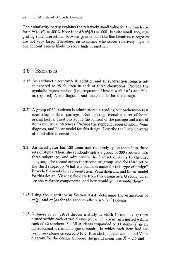
92 3. Multifacet G Study Designs

Their similarity partly explains the relatively small value for the quadraticform a2 (hIH ) = .0013. Note that a2 (phIH ) = .0051 is quite small, too, sug­gesting that interactions between persons and the fixed content categoriesare not very large. Therefore, an examinee who scores relatively high inone content area is likely to score high in another.

3.6 Exercises

3.1* An arithmetic test with 10 addition and 10 subtraction items is ad­ministered to 25 children in each of three classrooms. Provide thesymbolic representation (i.e., sequence of letters with "x"s and ":"s,as required), Venn diagram, and linear model for this design.

3.2* A group of 30 students is administered a reading comprehension testconsisting of three passages. Each passage contains a set of itemsasking factual quest ions about the content of the passage and a set ofitems requiring inferences. Provide the symbolic representation, Venndiagram, and linear model for this design. Describe the likely universeof admissible observations.

3.3 An investigator has 120 items and randomly splits them into threesets of items. Then, she randomly splits a group of 300 students intothree subgroups, and administers the first set of items to the firstsubgroup, the second set to the second subgroup, and the third set tothe third subgroup. What is a common name for this type of design?Provide the symbolic representation, Venn diagram, and linear modelfor this design. Viewing the data from this design as a G study, whatare the variance components, and how would you estimate them?

3.4* Using the algorithm in Section 3.4.4, determine the estimators of(J"2 (p) and (J"2 (h) for the random effects p x (i: h) design.

3.5* Gillmore et al. (1978) discuss a study in which 14 students (p) arenested within each of two classes (c), which are in turn nested withineach of 42 teachers (t) . All students responded to 11 items (i) in aninstructional assessment questionnaire, in which each item had sixresponse categories scored 0 to 5. Provide the linear model and Venndiagram for the design. Suppose the grand mean was X = 2.5 and

3.6 Exercises 93

L X~ = 269.4830 L L X~t = 545.9125t c t

L L L X~ct = 8229.2590 L X~ = 69.0028pe t i

L L X~i = 3003.0981 L L L X~it = 6111.2862t c i t

L L L L X;ict = 97506.4529.p et

Provide the degrees of freedom, T terms, sums of squares, meansquares, and est imated random effects variance components.

3.6 Consider the following scores for 10 students (p) on two science per­formance tasks (t ) with all responses scored by the same three raters(r).

t1 t2p rl r2 r3 rl r2 r31 3 2 1 4 3 12 3 1 1 4 1 13 3 3 3 4 2 24 3 2 1 4 2 15 3 2 2 4 2 26 3 3 2 4 4 27 3 3 2 4 4 38 3 1 0 4 1 09 3 4 1 4 4 110 3 2 2 4 3 3

Provide the degrees of freedom, T terms, sums of squares, meansquares, and est imated random effects variance components.

3.7* Consider the p x (i:h) design for the model M with np < Np < 00,

ni < Ni < 00, and nh < Nh < 00 .

(a) What are the expect ed mean squares for p, ph, and pi:h?

(b) What is (T2(phIM) in terms of random effects varian ce compo­nents ?

(c) Verify (b) given (a).

3.8 Consider, again , Synthetic Data Set No. 1 in Table 2.2, and supposethat persons 1 to 5 are in one dass, and persons 6 to 10 are in asecond dass.

(a) What is the G study design?

94 3. Multifacet G Study Designs

(b) What are the degrees of freedom, T terms, sums of squares,mean squares, and G study estimated random effects variancecomponents?

(c) What are the G study estimated variance components under theassumption that items are fixed-Le., ni = Ni = 127

(d) What are the G study estimated variance components under theassumptions that ne = 2 < Ne = 10, np = 5 < Np = 30, andni = 12 < Ni ---+ oo?

4Multifacet Universes of Generalizationand D Study Designs

In this chapter it is assumed that all facets in the universe of admissi­ble observations can be considered infinite in size and , consequently, theG study variance components have been estimated for a mndom model.Given these assumptions, this chapter provides procedures, equations, andrules for estimating universe score variance , error variances , generalizabilitycoefficients, and other quantities for random and mixed model D studieswith any number of facets. The random model equations and rules arequite general. The mixed model procedures are somewhat simplified; moregeneral procedures are treated in Chapter 5.

The substance of this chapter is at the very center of generalizability the­ory. In particular, considering multifacet universes of generalization forcesan investigator to draw careful distinctions among which facets are fixedand which are random for a measurement procedure. Such decisions af­feet both universe score variance and error variances . Also, the investigatormust consider D study sample sizes and D study design structure, both ofwhich affect error variances .

Some of the issues covered in this chapter overlap those in Chapter 2 forsingle-facet designs. To preclude frequent cross-referencing back to Chap­ter 2, there is some duplication of equations.

96 4. Multifacet D Study Designs

4.1 Random Models and Infinite Universes ofGeneralization

Linear models for multifacet D study designs can be specified using theprocedures discussed in Chapter 3 for G study designs, except th at for Dstudy designs an uppercase index is used if the index is associated witha facet in the universe of generalization. This notational convent ion em­phasizes that D study linear models are for the decomposition of observedmean scores for the objects of measurement over sets of condit ions (notsingle conditions) in the universe of generalization. Unless otherwise noted,persons are the objects of measurement in thi s chapter.

Consider , for example, the p x I x H design. The linear model for thedecomposition of a person 's observed mean scores over n~ and n~ condit ionsis

XpIH = J.1. + Vp + /11 + vn + Vpl + /lpH + /lIH + J.1.pIH , (4.1)

and the linear model associated with the p x (I :H) design is

XpIH = J.1. + /lp + vn + /lI :H + /lp H + /lpI :H' (4.2)

As in Chapter 2, we frequently use X p as an abbreviat ion for the meanfor a person over an sampled conditions of an facets , such as X pIH inEquations 4.1 and 4.2.

Each of the effects in linear models such as those in Equations 4.1 and4.2 can be expressed also in terms of a linear combination of populationand / or universe (of generalization) mean scores that define the effect . To doso, one simply uses the algorithm in Section 3.2.3, replacing any lowercaseindex with an uppercase index if the index is associated with a facet in theuniverse of generalization. So, for example, in terms of mean scores, the/lpH effect in both Equations 4.1 and 4.2 is

/lpH = J.1.pH - J.1.p - J.1.H + J.1. .

In short, linear models for persons' observed mean scores can be expressedexplicitly in terms of linear combinat ions of mean scores or, more com­pactly, in terms of score effects. In th is sense, linear models for D studydesigns are completely analogous to those discussed in Chapter 3 for Gstudy designs.

Since we are assuming in this section th at an effects are random (exceptJ.1.) , the linear models discussed here are mndom effects linear models withdefinitions and assumpt ions like those discussed in Sections 3.2 and 3.4.The only difference is that these definitions and assumpt ions now relate tomeans over sets of condit ions in the universe of generalization rather thansingle conditions in the universe of admissible observat ions. In particular,t he manner in which mean scores are defined implies that the expected

4.1 Randorn Models 97

value of any score effect is zero. For example, for both the p x I x Handp x (I :H ) designs,

J.LH:::::: EEXpIHp I

It follows th at

and J.L:::::: EEEXpIH.p I H

E VH :::::: E (J.LH - J.L) = E J.LH - J.L = o.H H H

Also, all effects are assumed to be uncorrelat ed. This is actu ally astrongerstatement than necessary in th at many pairs of effects are necessarily un­correlated by the manner in which they are defined in generalizability (seeBrennan, 1994; Exercise 4.2).

A particular D study design is associated with a rneasurement procedureand a universe of generalizat ion. Suppose, for example, that n~ = 5, n~ = 2,and the D study design is p x I x H . In this case, any single instance ofthe measurement procedure would result in persons' observed mean scoresassociated with a random sample of n~ = 5 condit ions from the i facetand an independent randorn sampie of n~ = 2 condit ions from the h facet ,and each person's observed mean score would be based on the averagescore over the same 10 pairs of sampled condit ions. Another instance ofthe same measurement procedure would simply involve a different randomsample of size n~ = 5 and n~ = 2 condit ions, using the same design. Theset of all such randomly parallel instances of the measurement procedureis analogous to the set of classically parallel forms in classical theory. Theset of all randomly parallel forms exhausts all condit ions in the universe ofgeneralization.

A particular D study design reflects the manner in which a measure­ment procedure is st ruct ured, but not necessarily the manner in which theuniverse of generalizat ion is st ructured. Especially for random models, itis quite common for a D study design to involve nesting of one or morefacets, although all facets are crossed in the universe of generalizat ion. Forexample, when items are nested within raters in a D study random effectsdesign, it is often the case that an investigator would allow any rater toevaluate any item, at least in principle. If so, the item and rater facetsare crossed in the universe of generalization (I x H) , and presum ably theinvestigator has chosen a nested design for practical reasons, or in order tomake the design efficient, in some sense.

4.1.1 Universe Score and Its Variance

Let R: be the set of random facets in the universe of generalization. Forrandom models, n exhausts the facets in th e universe of generalization,and the universe score for a person p is defined as

(4.3)

98 4. Multifacet D Study Designs

For example, when the facets are land H, the universe score for person pis

fLp ==EEXpIH .I H

That is, a person's universe (of generalization) score is his or her expectedscore over land H in the universe of generalization. Alternatively, a per­son's universe score is the expected value of his or her observable meanscore over all randomly parallel instances of the measurement procedure,each of which involves a different random sample of sets of conditions Iand H.

By convention , the universe of admissible observations is viewed as auniverse of single conditions of facets (e.g., i and h), while the universe ofgeneralization is usually viewed as a universe consisting of sets of conditionsof facets (e.g., land H). When the two universes are the same, except forthis distinction, it is clear that

fLp == EEXpIH = EEXpih .I H i h

(4.4)a2(p) == E (fLP - EfLP)2= Ev; .p p p

For random models, then, a trivial rule for identifying universe score vari­ance when persons are the objects of measurement is:

Rule 4.1.1: a2(p) is universe score variance .

However, it is misleading to think about universe score as an expected valueover conditions in the universe of admissible observations, because universescore is defined with respect to the universe of generalization. Universe scoreis interpretable as an expected value over instances of a measurement pro­cedure, and such instances are not defined until the investigator considersthe universe of generalization and D study issues.

The variance of the universe scores defined in Equation 4.3 is universescore variance:

Universe score variance, as defined in Equation 4.4, also equals the ex­pected value of the covariance of person mean scores over pairs of randomlyparallel instances of the measurement procedure, say, n and n' ; that is,

(4.5)

where the covariance is taken over persons , and the expectation is takenover pairs of randomly parallel forms. For example, consider the p x I x Hdesign. Let I and I' represent different random samples of size n; from onefacet , and let Hand H' represent different random samples of size nhfromthe other facet. Then, n includes these two facets (i.e., I/I' and H/H'),and

E a (XpIH , XpI' H')

4.1 Random Models 99

TABLE 4.1. Random Effects Variance Components that Enter (72(7), (12(0), and(12(ß) for Random and Mixed Model D Studies for the p x I x H Design

D Studies

(j2(ä) I ,H Random H Fixed" I Fixed"

(j2(p) T T 7

(j2(I) = (j2(i) /n~ ~ ~

(j2(H) = (j2(h)/nh ~ ~

(j2(pI) = (j2(pi) /n~ ~,8 ~,8 T

(j2(pH) = (j2(ph)/nh ~,8 T ~,8

(j2(IH) = (j 2(ih) /n~nh ~ ~ ~

(j 2 (pI H) = (j 2 (pih)/ n~nh ~,8 ~,8 ~,8

aDiscussed in Section 4.3.

TABLE 4.2. Random Effects Variance Components that Enter (12(7) , (12(0), and(12 (ß) for Random and Mixed Model D Studies for the p x (I :H) Design

D Studies

I ,H Random H Fixed"

(j 2 (p)(j2(H) = (j2(h)/ nh(j2(I:H) = (j2(i:h) /n~nh

(j2(pH) = (j2(ph) /nh(j2(pI:H) = (j2(pi :h) /n~nh

aDiscussed in Seetion 4 .3 .

T

7

~,8

E [ f (Vp + VpI + VpH + VpIH) X

(Vp + VpI' + VpH' + VpI' H') ] .

After formin g all the cross-products and taking expectations of them , allthat remains is Epv; = (j2(p) , the universe score variance.

It is especially important to not e that universe scores and universe scorevari ance are defined for the universe of generalization and do not depend onD study sam ple sizes or t he struct ure ofthe D study design [e.g., p x I x Hversus p x (I :H)]. By contrast , as discussed soon , error variances do de­pend on both D study sampIe sizes and design structure.

(4.7)

100 4. Multifacet D Study Designs

4.1.2 D Study Variance Components

In Chapter 3 the notation O'2 (a ) was introduced to designate variance com­

ponents associated with random effects in linear models for G study designs.For D study designs, the notation O'2 (ä ) is used to emphasize that D studyvariance components are associated with means for sets of sampled con­ditions.! For random models, obtaining the O'2(ä) from the O'2 (a ) is verysimple:

(4.6)

where

{

1 if ä = p, and, otherwise, the productd(ä) = of the D study sample sizes (n') for all

indices in ä except p.

Tables 4.1 and 4.2 provide equations for the O'2 (ä ) in terms of the O'2 (a)

for the p x I x Hand p x (I: H) designs, respectively. Consider, for ex­ample, O'2 (pH ) for either design. This variance component is the expectedvalue of the square of the VpH effects in the linear model for each design,where VpH is the average of the ~ph effects over n" conditions. Assumingscore effects are uncorrelated, it follows that

0'2 (pH) == EV;H = E [~~~Ph]2 O'2~~h) (4.8)

This sequence of equalities essentially states the well-known result that thevariance of a mean für a set of uncorrelated observations is the variance ofthe individual elements divided by the sample size (see Exercise 4.1). Nonormality assumpt ions are required to derive this result.

4.1.3 Error Variances

The two most frequently discussed types of error in generalizability theoryare absolute error and relative error. A third type is the error associatedwith using the overall observed mean to estimate the mean in the popu­lation and universe. All three of these types of errors were introduced inChapter 2 for single-facet universes and designs. They are extended hereto multifacet universes and designs for random models.

Absolute Error Variance

Absolute error for a person p is defined as

6.pn == X pn -Ilp , (4.9)

1As discussed in Chapter 2, in generalizability theory, the convention is to use themean-score metric, although the total-score metric could be used . This issue is discussedmore extensively in Section 7.2.5.

4.1 Random Models 101

which is often abbreviated

(4.10)

It is the error involved in using an examinee's observed mean score as anestimate of his or her universe score. Consider, for example the p x I x Hdesign in Equation 4.1. Since J.Lp = J.L + l/p, it follows from the definition inEquation 4.9 that

(4.11)

The expected value of D.p over the infinite facets in R: is zero; that is,

ED.pn = O.n

(4.12)

Clearly, for example, the expected value, over land H, of D.p in Equa­tion 4.11 is zero.

Absolute error variance is defined as

(4.13)

The term in square brackets is the error variance for a person p, calledconditional error variance, which is discussed in detail in Section 5.4. Here,we simply note that the overall D.-type error variance in Equation 4.13is interpretable as the expected value (over persons) of conditional errorvariance.? For example, the overall error variance associated with D.p inEquation 4.11 is

In terms of the notational system used here, it is easy to determine whichof the O'2(a) enter O'2(D.):

Rule 4.1.2: O'2(D.) is the sum of all 0'2(6:) except O'2(p) .

The second columns of Tables 4.1 and 4.2 report which variance compo­nents enter 0'2 (D.) for the random effects p x I x Hand p x (I: H) designs,respectively.

2Note that En is within the square brackets in the definition of (72(.:l) in Equa­tion 4.13 in order to express that definition as the expected value (over the population)of conditional error variance. Overall .:l-type error variance would be unchanged, how­ever, if the positions of the E p and En operators were interchanged.

102 4. Multifacet D Study Designs

Relative Error Variance

Relative error for a person p is defined as

(4.14)

which is often abbreviated

(4.15)

As such, op is the error associated with using an examinee's observabledeviation score as an estimate of his or her universe deviation score. Forthe p x I x H design,

EXp = J-t + 111 + IIH + IIIH = J-tIH ,p

and, therefore,

Op (Xp- J-tJH) -(J-tp- J-t)

IIpI + IIpH + IIpIH· (4.16)

The expected value of op over the population and / or over the infinite facetsin R is zero; that is,

E opn = E opn = O.p n

(4.17)

Clearly, for example, for op in Equat ion 4.16, the expected value over p iszero, and the expected value over l and H is also zero.

Relative error variance is defined as

(4.18)

Cronbach et al. (1972) designated relative error variance as Ea2(0), wherethe expectation E is taken over R. Although their notation is not usedhere, the definition in Equation 4.18 is consistent with the Cronbach et al.not ation in that E n is outside the square brackets . We return to this matterin the next section when we discuss expected observed score variance.

For the p x I x H design, op is given by Equation 4.16, and its varianceis

a 2(0) = a 2(pI) + a 2(pH) + a2(pI H )a2 (pi) a 2 (ph) a 2 (pih)

= -- +-- + -=----...:...n~ ni. n~ni. ·

The following rule can be used to obtain a 2 (0) for any random effectsdesign.

4.1 Random Models 103

Rule 4.1.3: (72(8) is the sum of all (72(&) such that & includes p andat least one oth er index.

In other words , (72(8) is the sum of all variance components that involveinteractions of p with facets in t he universe of generalizat ion. The secondcolumns ofTables 4.1 and 4.2 report which variance components ente r (72(8)for the random effects p x 1 x H and p X (1 :H) designs, respectively.

Comparing Absolute and Relative Error Variance

Absolute error variance is always at least as large as relative error variance.For example, for t he p x 1 x H design

and for t he p x (1 :H) design

(72(~) = (72(8) + (72(H) + (72(I:H) .

Assuming the universe of generalizat ion has 1 x H , the difference betweenabsolute and relative error variance for both designs is

because/-LI H - /-L = VI + VH + VI H = VH + VI :H ·

Absolute error variance takes into account the potential differences amongoverall means (/-LIH) for randomly parallel inst ances of a measurement pro­cedure. Ifthe /-LIH are all equal, then (72(8) and (72(~) are indistinguishable.The same kind of statement was made in Chapter 2 when classically parallelforms were discussed for single-facet universes.

The st ruct ure of a D st udy design influences the magnitude of errorvar iances. Suppose t he universe of generalizat ion is 1 x H , and consider t hep x 1 x H and p x (I :H ) design structures with ident ical sample sizes. Forthe p x 1 x H design,

By contrast , for t he p x (I :H) design ,

(72(ph) (72 (pi:h)---+--':-,.-'-

nh n~nh

(72 (ph) (72 (pi) (72(pih)--+--+-:=---:-...:...

nh n~nh n~nh'

since (72(pi:h) = (7 2(pi) + (72(pih) , as discussed in Section 3.2. Note that(72(pi) is divided by n~ when t he design is p x 1 x H , but it is divided by

104 4. Multifacet D Study Designs

n~n~ when the design is p x (I :H) . Therefore, all other things being equal,(12(0) is smaller for the p x (I :H) design than for the p x I x H design.A similar statement applies to (12(.6.). In this sense, for a fixed numberof observations per person , the p x (I: H) design is more efficient thanthe p x I x H design. This result is associated with the fact that, for thep x (I: H) design, the total number of sampled items is n~nh ' whereas onlyn~ items are involved in the p x I x H design-sampling more conditionsof facets tends to reduce error.

Error Variance for Estimating J.L Using X

Absolute error and relative error are, by far, the most frequently discussedand used, but other types of error may be of interest. For example, the errorvariance associated with using the observed grand mean X as an estimateof the mean in the population and universe f1. is

(4.19)

where XP'R = X is the D study mean over the observed levels of alt facets,including persons. That is why the person subscript in Equation 4.19 is anuppercase P. For random models, (12(X) can be obtained by first dividingeach (12(ä) by n~ if ä includes p, and then summing these with all other(12(&) . This verbal recipe is equivalent to the formula :

(12(X) = (12(p) : (12(0) + [(12(.6.) _ (12(0)] .P

(4.20)

Note, in particular, that (12(X) includes the universe score variance (12(p) .Alternatively, for random models, (12(X) can be obtained by first dividingeach of the (12(a) by the product of the D study sarnple sizes for indices ina, and then summing (see Exercise 4.3).

4.1.4 Coefficients and Siqnal-Noise Ratios

Traditionally, two coefficients predominate in generalizability theory, bothof which have a range of zero to one. A generalizability coefficient is verymuch like a reliability coefficient in classical theory. It employs relativeerror variance . A phi coefficient employs absolute error variance.

The basic equation for a generalizability coefficient for multifacet randomdesigns is the same as that for single-facet random designs:

(4.21)

Of course, the variance components that enter (12 (0) for multifacet designsare different from those that enter (12(0) for single-facet designs. This fact

4.1 Rand om Models 105

has consequences, many of which are illustrated in examples later in t hischapter . The symbolism E p2 used to represent a generalizability coeffi­cient highlights that it is interp ret able as an approximat ion to the squaredcorrelation between universe scores and observed scores.

The denominator of E p2 in Equation 4.21 is sometimes called expect edobserved score vari an ce and defined as

(4.22)

where X p = X pn , and t he E in E S 2(p) means t hat the expectation ist aken over t he set of random facets, R . For both this definiti on and t hedefinition of O'2(b') in Equ ation 4.18, the expectation over R is taken last .ES2 (p) is interpret abl e as the expected value over randomly par allel in­st ances of t he measurement pro cedure (i.e., R) of the observed vari ance forthe populati on. Given Equation 4.22 and Rule 4.1.3, it is evident that:

Rule 4.1.4: E S 2(p) is t he sum of all 0'2(&) t ha t include p.

The basic equation for an index of dependability, or ph i coefficient, is t hesame for mul tifacet des igns as it is for single-facet desig ns:

(4.23)

Of course, t he var iance components t hat enter O'2(ß) for mul tifacet de­signs are different from those that ente r O'2 (ß) for single-facet designs. Aphi coefficient differs from a generalizability coefficient only in that <I> in­volves absolute error variance rather t ha n t he relative error variance inE p2. Among ot her things, t his difference means t hat t he denomin ator of <I>is no t the observed variance for persons; it is the mean squared dev iationE (Xp - J.L )2 for persons.

The informat ion in the coefficients E p2 and <I> can be expressed as t hesignal-noise rati os

and

SjN(b') = O'2 (p)0'2(b')

(4.24)

(4.25)

respecti vely, which have limits ranging from zero to infinity. Relat ionshipsbetween E p2 and S/ N (b') are:

2 SjN (b' )Ep = 1 + SjN (b' ) and SjN(o) = E p

2 .1-Ep2

106 4. Multifacet D St udy Designs

Total Variance

FI GURE 4.1. Venn diag rarn representat ion of variance cornponents for thep x I x H design with both land H rand orn.

Corresponding relationships between <I> and S j N (!:i.)are:

SjN (!:i.)<I> = 1 +Sj N (!:i. ) and

<I>SjN(!:i.)=-,T,..

1- 'l.'

Kane (1996) discusses coefficients , signal-noise ratios, and a number ofot her measures of precision t hat might be applied in generalizab ility anal­yses. In par t icular , the error-to lerance ratios discussed in Section 2.5.1 forsingle-facet designs also apply to multifacet designs.

4.1 Randorn Models 107

2a (p )

Total Variance

2o (r)

FIGURE 4.2. Venn diagrarn representation of variance cornponents for thep x (I :H ) design with both l and H randorn.

4.1.5 Venn Diagrams

Figure 4.1 provides Venn diagram representations of variance componentsfor the p x 1 x H design, and Figure 4.2 provides the same type of infor­mation for the p x (1 :H ) design . For each figure, the full Venn diagram inthe upp er left-h and corner represents the so-called "total vari ance'lr'

-- 2 2E (Xp - /1) = E E (Xpn - /1)n: »

3Much of the generalizability theory literat ure uses th e phrase "total variance," butit is not total variance for persons ' mean scores ; rather, it is a mean-squ ared deviationfor persons.

108 4. Multifacet D Study Designs

and its decomposition. Note that total variance is not the same as (i2(X) inEquation 4.19 or ES2 (p) in Equation 4.22. The size of any particular areain these Venn diagrams does not reflect anything about its magnitude.

The upper right-hand corner of each figure represents (i2(L}.) as the fullVenn diagram excluding the universe score variance (i2(p) . The bottom halfof the two figures illustrates that the entire p circle can be associated withexpected observed score variance, which can be partitioned into universescore variance [designated (i2(r) at the bottom of the figures] and relativeerror variance. Comparing the Venn diagram representations of (i2(8) and(i2 (L}.) gives a visual perspective on the additional variance components thatenter (i2(L}.) , namely, all variance components outside the p circle. Theseadditional variance components represent contributions to total variancethat are const ant for all persons .

In comparing the Venn diagrams for the p x I x Hand p x (I :H) de­signs, note that

and(i2(pI:H) = (i2(pI) + (i2(pIH) .

Therefore, the areas associated with (i2(I:H) and (i2(p/ :H) in Figure 4.2represent the combination of two areas in Figure 4.1.

4.1.6 Rules and Equations fOT Any Object of Measuremeni

To this point in this chapter it has been assumed that persons are the ob­jects of measurement. In principle, however, any facet can play that role.Cardinet et al. (1976) refer to this fact as the "symmetry" of generaliz­ability theory. A common example occurs when students are nested withinclassrooms, and classes are the objects of measurement, that is, the unitsabout which decisions are made . No matter what objects of measurementare involved, the equations and rules discussed in this chapter still applyprovided the index p is replaced by the index representing the objects ofmeasurement.

Letting r be a generic index designating the objects of measurement, Ta­ble 4.3 summarizes the notation, rules, and most frequently used equationsfor random model D studies. The equation numbers in Table 4.3 correspondto those in the text. The only differences in the equations are that thosein Table 4.3 are expressed with respect to r , not p, and d(älr) is used inTable 4.3, rather than d(ä) .

These rules and equations assurne that the objects of measurement arenot nested within some other facet. Generalizability theory can treat suchnested, or stratified, objects of measurement , but to do so requires specialconsiderat ions (see Section 5.2).

In practical applicat ions, of course, the (i2(a) in Table 4.3 are replacedwith estimates, which are usually those discussed in Chapter 3. In doing

4.1 Random Models 109

TABLE 4.3. Rules and Equations for Random Model D Studies

Let 7 = obj ects of measurement.Let R = set of all random facets in universe of generalization .

D study vari ance components: 0-2(&) = 0-2(a)jd(&17)

{

I if & = 7 , and, otherwise, the productwhere d(( 17) = of the D st udy sample sizes (n') for all

indices in & except 7 .

Rule 4.1.1: 0-2(7) is universe score vari ance.Rule 4.1.2: 0-2 (~) is the sum of all 0-2(&) except 0-2(7).Rule 4.1.3: 0-2(<5 ) is the sum of all 0-2(& ) such that &

includes 7 and at least one other index.

0-2(X) = 0-2(7)

~ 0-2(<5 ) + [0-2(~) - 0-2(<5 )].

nT

E 2 _ 0-2(7)P - 0-2(7) + 0-2(<5 ) '

<I> = 0-2(7) .

0-2(7) + 0-2(~)

(4.6')

(4.7')

(4.20')

(4.21')

(4.23')

so, it is effect ively assumed that NT = N~ ........ 00 for t he obj ects of mea­surement. Even when this assumpt ion is clearly false, estimates of 0-2 (7) ,0-2(<5 ), and 0-2(~) are not likely to be much affected when the sample sizen~ is even moderately large.?

4.1.7 D Study Design Structures Different from the G Study

Equation 4.7 for det ermining D study variance components assumes thatthe structures of the G and D st udies are the same. Suppose, however , thatthe G study uses the p x i x h design , but the D st udy uses the p x (I :H)design . In this case, before using Equ ation 4.7 to obtain the d(&), the Gstudy vari ance component s for the p x (i :h) design need to be representedin terms of those for the p x i x h design. Doing so gives

and

4This is a very much different issue from what happens when a un iverse-of­generalization facet is fixed in the D study, as discussed lat er in Sectio n 4.3.

110 4. Multifacet D Study Designs

These equalities are basically exampies of the rule discussed in Section 3.2for determining which effects in a fully crossed design are confounded in aneffect from a design that involves nesting:

Confounded-Effects Rule: The effects that are confounded are allthose that involve onIy indices in the nested effect and that includethe primary index (indices) in the nested effect.

When botli the G and D study designs involve nesting, these steps canbe used:

1. use the confounded-effects rule to express each effect in the G studydesign in terms of effects from the fully crossed design;

2. use the confounded-effects rule to express each effect in the D studydesign (single-conditions-version) in terms of effects from the fullycrossed design; and

3. use 1 and 2 to determine, if possible.f which effects from the Gstudy design are confounded in effects for the D study design (singIe­conditions-version) .

For exampIe, suppose the G study uses the p x (i: h) design, but the Dstudy employs the I :H :p design, and we want to know what effects fromthe p x (i: h) design are confounded in the i:h :p effect. For the i :h :p design,

i:h:p ~ (i,ih ,pi,pih);

and for the p x (i: h) design,

i:h ~ (i, ih) and pi :h ~ (pi ,pih) .

It follows that (J2(i :h:p) = (J2(i :h) + (J2(pi:h).

4.2 Random Model Examples

In this section, both synthetic and real-data examples are used to illus­trate random model rules and procedures for D studies. These exampleshighlight some important differences between classical results and those ingeneralizability theory, and they demonstrate a few different ways of de­picting results numerically and graphically. The exercises at the end of thischapter provide additional instructive examples.

4.2.1 p X I X 0 Design with Synthetic Data Set No. 3

Table 4.4 reports resuits for D studies empIoying the p x I x 0 design,based on the G study estimated variance components for Synthetic Data

5It is not always possible to express effects for every nested design in terms of effectsfor another nested design (see Exercise 4.4).

4.2 Random Model Examples 111

TABLE 4.4. Ran dom Effects D Study p x I x 0 Designs For Synthetic Data 3

D Studies

n'on'

t

14

18

116

24

28

216

0-2(p) = .55280-2(i) = .44170-2(0) = .0074

0-2(pi) = .57500-2(po) = .10090-2(io) = .1565

0-2(pio) = .9352

0-2(p)0-2(1)

0-2 (0 )0-2(p1)

0-2(pO)0- 2 (10 )

0-2(pIO)

.553

.110

.007

.144

.101

.039

.234

.553

.055

.007

.072

.101

.020

.117

.553

.028

.007

.036

.101

.010

.058

.553

.110

.004

.144

.050

.020

.117

.553

.055

.004

.072

.050

.010

.058

.553

.028

.004

.036

.050

.005

.029

0-2(7)0-2(6)

0-2(~)

E ß2

<I>

.55

.48

.64

.54

.47

.55

.29

.37

.66

.60

.55

.20

.24

.74

.70

.55

.31

.45

.64

.55

.55

.18

.25

.75

.69

.55

.12

.15

.83

.78

One Occasion Two Occasions

t:.li t:. t:.

li 11 li lili li li

li li li li t:. t:. t:. t:. li11 li li li li

4 6 8 10 12 14 16Number of Items

0.9

0.8

0.7~UJ 0.6C/l

0.5

0.4

0.3, -+--,--,---,--.-...,....-,...-,.--,-~~---,.-....,........,24 6 8 10 12 14 16

Number of Items

0.5

0.4

0.3+-~~-.-...,.-,...-,.~~~---,.-....,........,

2

0.9

0.8

0.7~UJ 0.6C/l

0.9

0.8E·13 0.7<:'-s0.6u

0.5

o.4-+--r--T---"-...,......,.......,,........,.......,....""""-""-"--'-"""'-'2 4 6 8 10 12 14 16

Number of Iterns

0.9

0.8E·13 0.7<:'-g 0.6u

0.5

o.4-+-~---,.-...,......,.......,,........,.......,.......,....-,...-,.--,-.......-.

2 4 6 8 10 12 14 16Number of Iterns

112 4. Multifacet D Study Designs

Set No. 3 in Table 3.3 on page 74. At the top of Table 4.4, the first three Dstudies are for one occasion, and the next three are for two occasions. Forboth sets of D studies, n~ = 4,8 , and 16. These results can be obt ainedusing the equations and rules summarized in Table 4.3 on page 109.

The figures at the bottom of Table 4.4 provide graphs of 8'(8), 8'(~) ,

EjP, and ~ for one and two occasions with 4 :::; n~ :::; 16. Note that thefirst two figures report estimated standard errors of measurement (I.e., thesquare roots of the estimated error variances), rather than estimated errorvariances. Also, the symbol p means E p2 , not its square root."

These numerical and graphical results illustrate that

• relative error variance is smaller than absolute error variance ;

• a generalizability coefficient is larger than an index of dependability;and

• as sampie sizes increase, universe score variance is unchanged, errorvariances decrease, and coefficients increase.

An investigator might reasonably ask questions about which variancecomponents contribute the most to error . Clearly, the answer depends uponthe sample sizes, but 8'2(pIO) is generally large. Also, with only one or twooccasions, 8'2(pO) tends to be relatively large suggesting that the rank or­derings of persons' mean scores over one or two randomly selected occasionsis generally different from the rank orderings of the same persons ' meanscores for another one or two randomly selected occasions.

Apparent Similarities with Some Traditional ReliabilityCoefficients

The values of Eß2 for two occasions may appear conceptually similar totest-retest reliability coefficients-sometimes called coefficientsof stability­but this apparent similarity is misleading for two reasons. For the p x I x 0random effects design, generalization is over both sets of items and sets ofoccasions, whereas a test-retest correlation keeps items fixed in the sensediscussed later in Section 4.3. Also, the generalizability coefficients for twooccasions are for decisions involving mean scores over two administrationsof the same test . By contrast, a test-retest correlation provides an estimateof reliability for scores based on a single administrat ion of a test .

The values of E p2 for one occasion may appear conceptually similar tointernal consistency reliability coefficients, but again there is an importantdifference. Even with n~ = 1 occasion, results for the p x I x 0 randomeffects design are for generalization over occasions. By contrast, for internalconsistency coefficients, occasion is generally a fixed "hidden" facet , as

6Using p2 or E p2 renders a graph too confusing.

4.2 Random Model Examples 113

discussed more fully later in Sect ions 4.4.3 and 5.1.4. If genera lizat ion isintended to a broader set of occasions than the single occasion on whichdata are collected, t hen the random model coefficients with n~ = 1 aremore app ropriat e th an t radit ional measures of internal consiste ncy. Note,however , that estimating the random model coefficients requires a G studywith n o ~ 2, even when the D st udy uses n~ = 1.

Inapplicability of Spearman-Brown Formula

One of the principal results from classical test theory is the Spearm an­Brown formula for predicting reliability for forms of different lengths. Underth e assumpt ions of classical t heory, reliability always increases as test lengthincreases. Thi s is not necessarily t rue in genera lizability theory when th ereare two or more random facets.

Consider , for example, the D st udy in Table 4.4 for n~ = 2 and n;= 4,which gives E/J2 = .64. For a test twice as long, the Spearrnan-Brownformul a predicts th at

E ' 2 = 2(.64) = .78.p 1 + .64

By cont rast , the D study with n~ = 2 and n; = 8 gives E /J2 = .75. T his dis­crepancy is not attributable to rounding error. Using the Spearrnan-Brownformula has the effect of dividing alt variance components th at enter 0-2 (8)by th e same constant . For this example, th en, 0-2(pI) , 0-2(pO), and 0-2(pI O)are all divided by two, whereas generalizability theory leaves 0-2(pO) un­changed for any number of items. It follows th at th e Spearrnan-Brownformul a predicts a larger value for reliability (and a smaller relative errorvari ance) than that obtained using genera lizability theory. Except in t rivialcases, t he Spearrnan- Brown formula does not apply when generalizat ion isover more t han one facet .

4.2.2 p X (I :0 ) Design with Synthetic Data Set No. 3

The D st udy results in Table 4.5 are based on the G study est imated randomeffects variance components for Synthetic Dat a Set No. 3. For Table 4.5,however , t he design struct ure is p x (1:0), not p x I x O. Therefore, be­fore applying th e rules and equations for random model D st udies, t he Gst udy p x i x 0 variance components need to be converted to variance com­ponents for the p x (i :0) design in the manner discussed in Section 4.1.7and illust rated in Tab le 4.5.

The D st udy results in Table 4.5 illustrate the theoretical arguments inSection 4.1.7. For exam ple, for the random model p x I x 0 design withn~ = 2 and n; = 4, Tab le 4.4 reports that

and Efl = .64.

114 4. Multifacet D Study Designs

TABLE 4.5. Random Effects D Study p x (I :0) Designs For Synthetic Data 3

D Studies

a-2 (a) for a-2 (a) for n' 1 1 2 20

p xi xo p x (i :o) n' 4 8 4 81

a-2 (p) = .5528 a-2 (p) = .5528 a-2 (p) .553 .553 .553 .553a-2

( 0 ) = .0074 a-2( 0 ) = .0074 a-2 (0 ) .007 .007 .004 .004

a-2( i) = .4417 } a-2(i:o) = .5982 a-2 (1:0) .150 .075 .075 .037a-2 (io) = .1565

a-2 (po) = .1009 a-2 (po) = .1009 a-2 (pO) .101 .101 .051 .051

a-2(pi) = .5750 } A2( '. ) = 1 5102 a-2 (pI :0 ) .378 .189 .189 .094A2( io) 9352 (J" pt:o .

(J" PW = .

a-2(r) .55 .55 .55 .55a-2 (8) .48 .29 .24 .15

a-2(L\) .64 .37 .32 .19E p2 .54 .66 .70 .79

<I> .47 .60 .63 .75

By contrast, for the same sample sizes, the random model p x (1: 0) designin 1Lable 4.5 gives

0-2 (0) = .24 and E p2 = .70.

That is, all other things being equal, the nested design leads to smallererror variances and , hence, larger coefficients.

Coefficients of Equivalence a nd Stability

The two D studies with n~ = 1 in Table 4.5 for the p x (1:0) designgive identical results to the corresponding D studies in Table 4.4 for thep x I x 0 design. When n~ is a single randomly selected occasion, there isno functional difference between the two designs, and occasion is a "hidden"random facet for both of them. (Hidden facets are discussed more fully laterin Section 5.1.4.)

Data collected using a G st udy p x (i :0) design with no = 2 admin­istrations are often used to estimate reliability in the classical sense of"equivalence and stability." Such a reliability coefficient is est imated bythe correlation between persons ' scores for the two administrations. Thiscorrelat ion involves neither the same items nor the same occasions, and itis an estimate of reliability for a single administration. The refore, it cor­responds conceptually with a generalizability coefficient for random effectsp x (1:0) (or p x I x 0) design with n~ = 1. Indeed, the expected valueof the numerator of the correlat ion (i.e., t he covariance) is the universe

4.2 Random Model Examples 115

score variance, as discussed in Section 4.1.1. There is a difference in th edenominators, however , because a correlat ion uses the geometrie mean ofthe two variances, whereas a generalizability coefficient uses th e expectedobserved score variance (l.e., an arit hmet ic mean) .

4.2.3 p X (R :T) Design with Synthetic Data Set No. 4

Table 4.6 reports results for six D studies using th e p x (R :T) design,based on th e G study est imated variance components in Table 3.4 for th ep x (r :t) design and Synthet ic Dat a Set No. 4. For this D study design,it is important to not e that since rat ers are nested within tasks, examineeresponses to each of th e n~ t asks are evaluated by a different set of n~

rat ers , and the total number of ratings for each examinee is n~n~ . 7

Table 4.6 reports results for all th e possible random effects D studies suchthat n~ :::; 6 and n~n~ is as elose as possible to 12 without exceeding it . Atth e bottom of th e table are "box-bar" plots that graphically summarizest atistics for the various D st udies in the manner illustrat ed in Figure 4.3.8

In these plot s, th e height of the solid box represents est imated universescore variance, and th e magnitudes of 0-2(8) and 0-2(ß) are represented byth e lengths of the bars below the box.

An investigator might examine th e D study results in Table 4.6 if timeand/or cost constraints required using no more th an six tasks and no moreth an 12 ratings per examinee. Clearly, both 0-2(ß) and 0-2(8) change evenwhen the total number of ratings remains constant at 12. Also, using moretasks leads to greater reduction in error variance th an using more rat ers pertask. For example, when n~ = 2 and n~ = 6, 0-2(ß) = .70; whereas whenn~ = 6 and n~ = 2, 0-2(ß) = .40. Under th e const raint th at n~n~ :::; 12, th eD studies in Table 4.6 indicate that error variance is minimized by usingsix tasks with two rat ers per task. However, th e investigator might alsoobserve th at error variances for five tasks are not much larger than thosefor six tasks, and the results for five tasks require a total of only 10 ratingsper examinee, as opposed to 12. This might lead th e investigat or to useonly five tasks.

Table 4.6 also reports th at :

• EiP = .50 for two tasks with six rat ers per task- a total of 12 ratingsper examinee; while

7This does not necessaril y rnean t hat t he universe of genera lization has R: T ; it iscertainly possible t hat the universe has R x T .

8T he generic Venn d iagrarn in Figure 4.3 do es not represent each of th e indiv idualD study vari an ce cornponents . Rat her, it depicts the relat ionships arnong un iverse scorevarian ce, relat ive error var iance , and absolute erro r vari an ce, with (}"2(R.) = (}"2 (f1)_(}"2 (8)being the set of a ll D st udy variance cornpo nents t hat includc indices for randorn facet sonly. For t he pa rticular box-bar plot in Figure 4.3 , E p2 = 32/40 = .80 an d cI> = 32/52 =.62.

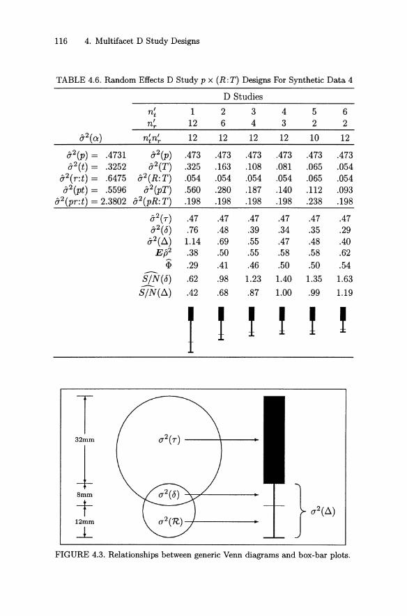
116 4. Mult ifacet D Study Designs

TABLE 4.6. Random Effects D Study p x (R :T) Designs For Synthetic Data 4

D Studies

n' 1 2 3 4 5 6tn' 12 6 4 3 2 2r

a-2 (a ) n~n~ 12 12 12 12 10 12

a-2 (p) = .4731 a-2(p) .473 .473 .473 .473 .473 .473a-2 (t ) = .3252 a-2 (T ) .325 .163 .108 .081 .065 .054

a-2 (r:t ) = .6475 a-2 (R:T ) .054 .054 .054 .054 .065 .054a-2(pt ) = .5596 a-2(pT ) .560 .280 .187 .140 .112 .093

a-2 (pr:t ) = 2.3802 a-2(pR:T ) .198 .198 .198 .198 .238 .198

a-2( 7 ) .47 .47 .47 .47 .47 .47

a-2(8) .76 .48 .39 .34 .35 .29a-2 (ß ) 1.14 .69 .55 .47 .48 .40

E/P .38 .50 .55 .58 .58 .62

il> .29 .41 .46 .50 .50 .54-§.LN(8) .62 .98 1.23 1.40 1.35 1.63

8jN(ß) .42 .68 .87 1.00 .99 1.19

I ! ! ! ! !

T32m m (T2(7)

1} U2(~)

8m m

T12mm

--LFIGURE 4.3. Relationships between generic Venn diagrams and box-bar plots.

4.2 Random Model Examples 117

• Eß2 = .58 for five tasks with two raters per task- a total of 10 ratingsper examinee.

In other words, for these sampie sizes, decreasing the total number of rat­ings per examinee leads to an increase in reliability. Such a result cannotoccur in any single applicat ion of classical theory with its undifferentiatederror term , but it can arise in generalizability theory when there is moreth an one source of rand om error.

This paradoxical result (from the perspective of classical theory) is a di­reet consequence of the fact that (j-2(pt) is relatively large, and its influenceon (j-2(8) decreases as the number oftasks increases, no matter what changesoccur for n~. In this particular example, the slight increase in (j-2(pR:T) asn~n~ goes from 12 to 10 does not offset the sizeable decrease in (j-2(pT) asn~ goes from two to five.

There are several lessons to be learned from this example and the previ­ous ones in this chapter. First , generalizability theory allows for, and indeedencourages, a multidimensional perspective on error variances. Second, tounderstand error variances, one needs to consider both the variance com­ponents th at enter them and D study sample sizes. Third, conventionalwisdom based on classical theory and single-faceted universes frequentlydoes not apply in generalizability theory. This does not mean that classicaltheory is wrong and generalizability theory is right in a universal sense, butit does mean that a single applicat ion of classical theory cannot differentiateamong the contribut ions of multiple sources of error.?

4.2.4 Performance Assessments

Generalizability theory is part icularly weil suited to evaluating assessmentsthat are based on ratin gs of human performance. The use of generalizabilitytheory in performance assessments in educat ional measurement has beenst udied by Brennan (1996b, 2000b), Brennan and Johnson (1995), Cron­bach et al. (1997), and Kane et al. (1999), among others.

Shavelson et al. (1993, p. 222) provide an instructive example of a per­formance assessment program in science called the California AssessmentProgram (CAP) . They state that:

Students were posed five independent tasks. More specifically,students rot ated through aseries of five self-contained stationsat t imed intervals (about 15 mins.) . At one stat ion, students

9Gulliksen (1950, pp . 211-214) dise usses reliability of essay seores from a c1assicalpe rspective, an d Hoover and Bray (1995) outline how c1assical t heory ean be used toexamine mult iple sourees of error in essay exa minations. Isolat ing t he sourees requiresmult iple analyses of different data sets or different subsets of t he same data set . In t hissense t he proeess is som ewhat disjointed and not nearly as int egrated and "rieh" as t heapproach in generalizability t heory.

118 4. Multifacet D Study Designs

were asked to complete a problem solving task (determine whichof these materials may serve as a conductor). At th e next sta­t ion, students were asked to develop a classification system forleaves and then to explain any adjustments necessary to in­clude a new mystery leaf in the system. At yet another, st udentswere asked to conduct tests with rocks and then use the resultsto determine the identity of an unknown rock. At the fourthstation, students were asked to est imate and measure variouscharacteristics of water (e.g., temperature , volume). And at thefifth station, students were asked to conduct aseries of testson samples of lake water to discover why fish are dying (e.g., isthe water too acidic?) . At each stat ion, students were providedwith the necessary materials and asked to respond to aseriesof quest ions in a specified format (e.g., fill in a table).

A predetermined scoring rubric developed by teams of teach­ers in Califomia was used to evaluate th e quality of students'written responses . . . to each of the tasks, Each rubric was usedto score performance on a scale from 0 to 4 (0 = no at tempt ,1 = serious flaws, 2 = sat isfactory, 3 = competent, 4 = out­st and ing). All tasks were scored by three raters.

For the CAP, the G study design is p x t x r with nt = 5 tasks andnr = 3 raters. We assurne here that tasks and raters are both random.Table 4.7 reports the G st udy est imated variance components, along withD studies for various sample sizes.

The G st udy est imated variance component for persons O'2 (p) = .298 isrelatively large, but the est imated variance component for the pt interac­tions a2 (pt ) = .493 is even larger. By contrast, a2 (r ), 0'2 (pr) , and a2(rt )are all elose to zero, which suggests that the rater facet does not cont ributemuch to variability in observed scores. Also, since O'2 (t ) = .003, it appearsthat tasks are quit e similar in average difficulty.

The CAP G study result s are typ ical of generalizability results for manyprograms that involve performance assessments; that is, 0'2 (pt) t ends to berelatively large, the rater facet often cont ributes relatively little variance,and O' 2 (t ) is often small. As discussed by Brenn an (1996b) , other publishedst udies using the p x t x r design that give similar result s include scienceand math assessments discussed by Shavelson et al. (1993) and tests oflistening and writing discussed by Brennan et al. (1995).

The D st udy results at the top of Table 4.7 illustrate that using threeraters gives very little improvement in measurement precision over t hatobtained using two raters, and the figures at the bottom suggest th at asingle rater may be adequate for many purposes. However, it is very elearthat t he number of tasks has a substant ial impact on error variances andcoefficients , which is to be expected since O'2 (pt ) is quite large.

4.2 Random Model Examples 119

TABLE 4.7. Random Effects D Study p x T x R Designs For CAP Data

D Studies

a-2(p) = .298a- 2(t ) = .092a-2 (r ) = .003

a-2 (pt) = .493a-2 (pr ) = .000a-2 (tr ) = .002

a-2 (ptr ) = .148

n'tn'r

a- 2 (p)a-2 (T )a-2 (R)

a-2 (pT )a- 2(pR)

a- 2 (TR)a- 2(pTR)

a-2(T)a-2 (6)

a-2(ll)Ep~

<I>

51

.298

.018

.003

.099

.000

.000

.030

.30

.13

.15

.70

.67

52

.298

.018

.002

.099

.000

.000

.015

.30

.11

.13

.72

.69

53

.298

.018

.001

.099

.000

.000

.010

.30

.11

.13

.73

.70

101

.298

.009

.003

.049

.000

.000

.015

.30

.06

.08

.82

.80

102

.298

.009

.002

.049

.000

.000

.007

.30

.06

.07

.84

.82

103

.298

.009

.001

.049

.000

.000

.005

.30

.05

.06

.85

.82

• 1 Rater

• 2 Raters

0.20+-...,.-...,.--r--r---r---r---r---r---r--,o 1 2 3 4 5 6 7 8 9 10

Number01 Tasks

0.90

0.80

~lli 0.70

g0.60w~ 0.50<51l0.40<Cl:

0.30

0.20+--r--r---r---r---r---r--r-r-r-,o 1 2 3 4 5 6 7 8 9 10

Number01 Tasks0.85

0.90

0.80

mO.70cne0.60w~ 0.50~äi 0.40CI:

0.30

0.85

• 1 Rater

• 2 Raters

I I

0.75

~ 0.65·u:E:~ 0.55oif 0.45

0.35

• 1 Rater

• 2 Raters

~ 0.75·u

~ 0.65o>.~ 0.55:ci

~ 0.45Q;c<3 0.35

• 1 Rater

• 2 Raters

0.25+-...,.--,----,---,---.---.--r-r---r--,o 1 2 3 4 5 6 7 8 9 10

Number01 Tasks

0.25+-...,....-...,....--,---r--r---r---r---r---r--,o 1 2 3 4 5 6 7 8 9 10

Number01 Tasks

No te. G study estimated vari ance co mpo nents were provided by Xiaoho ng Gao.

120 4. Multifacet D Study Designs

The Shavelson et al, (1993) study does not include all potentially rele­vant facets. For example, the occasion on which tasks were administeredwas not varied. Therefore, their study does not permit generalizing to dif­ferent testing occasions. This limitation may be quite important in that theliterature contains some evidence that the relatively large value of (J'2 (pt)is sometimes better characterized as (J'2(ptO) (see Ruiz-Primo et al., 1993;and Webb et al., 2000).

In many performance assessments, there are other facets that may beimportant but are frequently overlooked, including the following.

• Rating occasions: The occasion on which ratings are obtained is oftendifferent from the occasion on which task responses are obtained. Thishappens, for example, when examinee responses are cent rally scored.That is, there are often two occasion facets: testing occasion andrating occasion. There is evidence that the rating occasion facet cancontribute significantly to error (see Wainer, 1993).

• Scoring rubrics : In almost all performance assessments, only one scor­ing rubric is used. However, there are often other rubrics that couldhave been used.

• Modes of testing: Most performance assessments involve only onemethod or mode of testing (e.g., actual performance observed byraters, videotaped performance, performance results recorded in anotebook, etc .). In the absence of evidence to the contrary, there isno compelling reason to believe that scores would be invariant overmodes of testing.

It is not always the case that these other facets (especially rubrics andmodes of testing) are best viewed as random. An investigator might viewone or more of them as fixed, using the methodology discussed in Sec­tion 4.3.

4.3 Simplified Procedures for Mixed Models

Thus far in this chapter it has been assumed that all facets in both theuniverse of admissible observations and the universe of generalization areinfinite in size. Frequently, however, an investigator wants to consider arestricted universe of generalization, that is, a universe of generalizationthat involves only a subset of the conditions in the universe of admissibleobservations.l" In such cases, the procedures discussed in this section canbe used provided certain conditions prevail:

10 A more elegant way to conceptualize a restricted universe is considered in Section 4.5.

4.3 Mixed Models 121

1. t he est imated G study varia nce components are for a random model,and

2. each facet in t he D st udy is either random or fixed , in the sensediscussed next .

If these condit ions do not apply, t hen the procedures in Secti on 5.1 can beused .

Recall that n rep resents t he G study sample size for a facet , and Nrepresents t he size of t he facet in the universe of admissible observat ions .Similarl y, n' represents t he D st udy sample size for a facet , and N ' repre­sents t he size of t he facet in the universe of generalizatio n. We say t hat afacet is fix ed in t he D st udy when n' = N ' < 00. This definition involvestwo considerat ions: t he number of condit ions for the facet in the universeof generalization is finite (N' < 00), and the D st udy sample size equalsthe number of condit ions for the facet in the universe of genera lizat ion(n' = N '). Fur thermore, since t he condit ions in t he D st udy must be con­tained in the universe of generalizat ion, it follows t hat t he condit ions oft he fixed facet in t he D st udy must be the sam e conditions as t hose in t heuniverse of generalization.

In genera lizability t heory it is always assumed t hat , for at least one facet ,generalization is intended to a larger universe of condit ions t han t hoseactually represented in the D st udy. If that were not t he case, t here wouldbe no errors of measurement , by definiti on! In this sect ion, it is assumedthat for every facet n' < N' -t 00 or n' = N' < 00, and for at least onefacet n' < N' -t 00. In t radit ional ANOVA terminology, therefore, thissection t reats mixed models.

4.3.1 Rules

For mixed models, a simp le set of equat ions and rules can be used to obtainuniverse score var iance, error variances, and coefficients. These equat ionsand rul es are based on using t he same u 2 (Q:) as t hose discussed in Sec­tion 4.1 for random models. That is, here we use D st udy random effectsvarian ce components t o obtain results for mixed models. This apparentincongruity means that these simplified procedures have limitations. How­ever , t hese simplified procedures are quite adequate for much practic alwork, and they provide an instruct ive basis for comparing error variancesand coefficients for random and mixed mod els.

T he not ation and equat ions summ ar ized in Table 4.3 on page 109 st illapply, but the rul es in Tab le 4.3 need to be alte red for mixed models. Formixed mod els, an observed mean score might be represented as X pR.F ,

where :F is t he set of fixed facets in the universe of generalization . Rec­ognizing that 'R. cont ains only random facets, t he rules for mixed modelsare:

122 4. Multifacet D Study Designs

Rule 4.3.1: a2(7) is the sum of all a2(&) such that & includes 7 anddoes not include any index in R;

Rule 4.3.2: a 2(ß ) is the sum of all a 2(&) such that & includes at leastone of the indices in R ; and

Rule 4.3.3: a2(8) is the sum of all a 2 (&) such t hat & includes 7 andat least one of the indices in R .

Tables 4.1 and 4.2 on page 99 illust rate these rules for mixed models withthe p x 1 x H and p x (I: H) designs, respectively.

To get a somewhat intui tive notion of why Rules 4.3.1 to 4.3.3 work, itis helpful to consider the expected mean squares for different models (seeSection 3.5). For example, for the p x (I :H) design,

EMS(p) a2(pi:h) + nia2(ph) + ninha2(p)

= a2(pi:hIH) + ninha2(pI H),

a2(pIH) = a2(p)+ a2(ph)

,nh

where a2(pIH) is universe score variance, a2(7), for the mixed model whennh= nh. This result is ident ical to th at obtained using Rule 4.3.1.

where the first equat ion is for the random model , and the second is for themixed model with H fixed. Since EMS(pi :h) = a2(pi:h) = a2(pi:h IH), itfollows that

4.3.2 Venn Diagrams

Visual perspectives on the p x 1 x H and p x (1 :H) designs with H fixedare provided by the Venn diagrams in Figure 4.4 and Figure 4.5, respec­tively. Figure 4.4 for the p x 1 x H design with H fixed can be comparedwith Figure 4.1 for the same design with both Hand 1 random . Note that ,with H fixed, a 2 (ß ) does not include a 2 (H ) because every inst ance of themeasurement procedure would contain the same nhcondit ions. Also, notethat the expected observed score variance is the same whether or not His fixed. What changes is the manner in which ES2(p) is decomposed intoa2 (7) and a2 (8). Specifically, when H is fixed, a2(pH) cont ributes to uni­verse score variance rather th an a 2 (8). In short , restricting the universe ofgeneralizat ion leads to an increase in universe score variance and a decreasein relative error variance, as compared to the random model results. Thesame conclusions are evident in comparing Figure 4.5 for the p x (I :H )design with H fixed with Figure 4.2 for the same design with both H and1 random.

It is evident from Tables 4.1 and 4.2, and from Figures 4.4 and 4.5, thatuniverse score variance for both the p x 1 x H and p x (1: H) designs is

a2(7 ) = a2(p) + a2(pH)

4.3 Mixed Models 123

Total Variance

2a Cr)

FIGURE 4.4. Venn diagram representation of variance components for thep x I x H design wit h I random and H fixed .

when H is fixed . In general, for a specified universe of generalizat ion, uni­verse score variance is unaffected by the structure of the D study. However ,error variances are affected. For example, suppose the universe of general­ization has I x H. If the D study design has H fixed, then for the p x I x Hdesign ,

Clearly, a 2 (0) is smaller for the p x (I :H) design with H fixed. A similarst at ement holds for a2(ll ). Recall from Section 4.1 that the same conclu­sions hold for random models. So, in general, all other things being equal,nest ed designs lead to smaller error variances than crossed designs.

124 4. Multifacet D Study Designs

Total Variance

FIGURE 4.5. Venn diagram representation of variance components for thep x (I: H) design with Irandom and H fixed.

The simplified procedures for mixed models based on Rules 4.3.1 to 4.3.3are very useful, but they have limitations. In particular, they use randomeffects D study variance components , rather than the D study componentsfor the actual mixed model. This deficiency is remedied by the proceduresin Section 5.1. Also, when these rules are used in practice, with parametersreplaced by estimates, strictly speaking it must be assumed that the G andD studies contain the same levels ofthe fixed facet(s) , not simply the samenumber of levels. Under these circumstances, the simplified procedures andthose in Section 5.1 give the same unbiased estimates of universe score vari­ance, error variances, and coefficients. If the G and D studies do not containthe same conditions, then the mixed model estimates are approximationsonly.

4.4 Mixed Model Examples 125

4.4 Mixed Model Examples

In this section, both synthetic and real-data examples are used to illustratethe simplified mixed model procedures in Section 4.3. Many aspects of theseexamples focus on differences between random and mixed model results.Particular emphasis is placed on illustrating how some classical reliabilitystatistics are interpretable from the perspective of random and/or mixedmodel results in generalizability theory, how the reliability of dass meansis easily accommodated in generalizability theory, and how generalizabilitytheory provides an elegant explanation of the reliability-validity paradox.The exercises at the end of this chapter provide additional instructive ex­amples .

4.4.1 P X I X 0 Design with Items Fixed

Section 4.2.1 treated random model D studies for the p x I x 0 design,based on the following G study estimated variance components for Syn­thetic Data Set No. 3.

O'2(p) = .5528O'2(pi) = .5750

O'2 (i ) = .4417O'2 (po) = .1009

O'2(pio) = .9352.

0'2(0) = .0074O'2 (io) = .1565

Now let us consider the p x I x 0 design for sample sizes of n~ = 2 andn~ = 4 with items fixed. Using Rules 4.3.1 to 4.3.3 on page 122 and theequations in Table 4.3 on page 109 , it is easy to verify the mixed modelresults in the first row of the following table.

I fixed .701,0 random .55

.17

.31

Est[ES2 (p)]

.86

.86.19.45

.81

.64.79.55

These mixed model results in the first row can be compared with the pre­viously discussed random model results in the second row. (For both rows,n~ = 2 and n~ = 4.) Clearly, fixing items leads to decreased error variancesand increased coefficients, as theory dictates. Note, also, that expectedobserved score variance is the same for both models. For a given designstructure and sample sizes, fixing a facet affects which variance compo­nents contribute to 0'2(7) and 0'2(0) , but it does not change their sum,

4.4.2 p X (R: T) Design with Tasks Fixed

Section 4.2.3 considered the p x (R :T) design for Synthetic Data Set No. 4under random model assumptions. Suppose , however, that an investigatoralso wants to consider a mixed model in which generalization is over raters,

126 4. Multifacet D Study Designs

TABLE 4.8. D Studies for p x (R :T) Design for Synthetic Data Set No. 4 UnderRandom Model and Model with Tasks Fixed

D Studies

n' 3 3 3 3tn' 1 2 3 4r

0-2(0:) n~n~ 3 6 9 12

0-2(p) = .4731 0-2(p) .473 .473 .473 .4730-2(t) = .3252 0-2(T) .108 .108 .108 .108

0-2(r:t) = .6475 0-2(R:T) .216 .108 .072 .0540-2 (pt ) = .5596 0-2(pT) .187 .187 .187 .187

0-2(pr:t) = 2.3802 0-2 (pR:T ) .793 .397 .265 .198

Model Ran Tf Ran Tf Ran Tf Ran Tf

0-2(7) .47 .66 .47 .66 .47 .66 .47 .660-2(0) .98 .79 .58 .40 .45 .26 .39 .200-2(~) 1.30 1.01 .80 .51 .63 .34 .55 .25

Est [ES2(p)] 1.45 1.45 1.061.06 .92 .92 .86 .86Eß2 .33 .45 .45 .62 .51 .71 .55 .77~ .27 .40 .37 .57 .43 .66 .46 .72

I! ! ! ! , ! ,Note. In the lower half of the t able , t he first ent ries are for a random model (Ran) , an d

the second ent ries are for a mod el with tasks fixed (TI )'

but not tasks. That is, the investigator is also interested in a universe ofgeneralization in which the same tasks would be used for every inst ance ofthe measurement procedure. Table 4.8 provides D study results for boththe random and mixed models under th e assumpt ion that n~ = 3, which isthe same numb er of tasks as those in th e synthet ic dat a.

For the mixed model results with T fixed and only one random facet (R) ,as the number of rat ers increases, error variances decrease and coefficientsincrease. By comparison with the random model , under the mixed model:

• universe score variance is larger,

• error variances are smaller,

• expected observed score variance is unchanged, and

• coefficients are larger.

4.4 Mixed Model Examples 127

These differences are predictable from t heory. The principal explanationis that , for the random model, a-2 (pT ) is part of error variances, whereasa-2 (pT ) cont ributes to universe score variance for t he mixed model with Tfixed.

The D study results for n~ = 1 in Table 4.8 require careful consider­ation. These results are est imates for a measurement procedure havingn~ = 3 tasks with each one evaluated by a single different rater. Clearly,if such dat a were analyzed , the task and rater facets would be completelyconfounded, and it would be impossible to treat raters as random and tasksas fixed . Doing so is possible here because a G st udy was conducted thatinvolved multiple raters and multiple t asks, which permits us to untanglethe cont ribut ions of the task and rat er facets.

4.4.3 Perspectives on Traditional Reliability Coeffici ents

In classical theory, three types of reliability coefficients are frequently dis­cussed:

• Stabilit y and equivalence: correlat ion for scores for different forms ofa test administe red on different occasions;

• St ability or test -retest : correlation of scores for the same form of atest administe red on different occasions; and

• Internal consistency: Cronbach's alpha or KR-20 based on a singleadminist rat ion of a test form.

Table 4.9 provides a genera lizability theory perspective on these coeffi­cients. Int ernal consistency coefficients are discussed more fully in Sec­tion 5.1.4, but the t heory discussed thus far is a sufficient basis for t hemost important distin ctions among t hese coefficients.

Relationships Among Coefficients

These t hree traditional coefficients are est imates of reliability for a singletest form, that is, a form administe red on a single occasion. That is why theD study sampie size for occasions is n~ = 1 for all coefficients, even thoughthe dat a collect ion design (G study) may involve two administrations. Toemphasize th at n~ = 1, a lowercase 0 , rather th an 0 , is used in the D studynot ation in Table 4.9. Second , the coefficients differ with respect to whichfacets are fixed and which are random in the universes of generalization.For a coefficient of stability and equivalence, both occasion and items arerand om; for a coefficient of st ability, items are fixed; and for an internalconsiste ncy coefficient there is a single fixed occasion .

The denominators (expected observed score variance) of the coefficientsin Equations 4.26 to 4.28 are all the same. So, differences in their nu­merators (universe score variance) will dictate relationships amon g them.

128 4. Multifacet D Study Designs

TABLE 4.9. Some Classical Reliability Coefficients from th e Perspect ive of Gen­eralizability Theory

Stability and Equivalence: Cerrelat ion of scores for different forms of atest administered on two different occasions.

G Study:

D Study:

p x (i :o)

p x (1:0)

no = 2

n~ = 1 (random); 1 random

a2(p) + [a2(po) + a2(p1 :0)]

a 2 (p)(4.26)

Stability: Correlation of scores for the same form of a test administe redon two different occasions.

G Study:

D Study:

p x i x 0 n o = 2

P x 1 x 0 n~ = 1 (random); 1 fixed

(4.27)

Internal Consistency (Equivalence) : Cronb ach's alpha or KR-20 basedon a single administ rat ion of a test form.

Not e. To conceptualize an internal consistency estimate of reliabilityand relate it to other coefficients, it is helpful to view th e universe ofadmissible observat ions as having an occasion facet , with a G st udyinvolving the collect ion of dat a on two or more occasions.

G Study: p x i x 0 or p x (i :0) no ~ 2

D Study: p x 1 x 0 or p x (I :0) n~ = 1 (fixed) ; 1 random

(4.28)

(4.29)

(4.30)

4.4 Mixed Model Examples 129

Clearly, a coefficient of equivalence and stability is likely to be smallerthan eit her of the other two. Astability coefficient will be smaller than aninternal consistency coefficient if a2(pI) < a2(po), which is highly likelywhenever n~ is large. These conclusions are in accord with experience; thatis, almost always,

Similarly, almost always,

Interrater Reliability

Int err at er coefficients are another frequently discussed type of reliability.Actually, there are at least two interrater coefficients, both of which areoften misunderstood:

• Standardized: correlation between the scores assigned by the sametwo raters to st udent responses to the same task; and

• Nonstandardized: correlation between the scores assigned by the sametwo raters to st udent responses to different tasks.

The magnitudes of standardized coefficients are often quite high, whilenonstandard ized coefficients tend to be small. As discussed by Brennan(2000b), these results are predictab le from a careful considerat ion of the Dstudy designs, sampie sizes, and universes of generalization that are implicitin these two coefficients .

In the te rminology of genera lizability theory, the standardized coefficientuses the G study p X t X T design with nr = 2 raters evaluating the sament = 1 task. For the D study, the design is p x t x r with a single randomrater and a single fixed task. It follows that the standardized coefficient is

E2 a2(p) + a2 (pt)

p -- a2 (p) + a2(pt) + [a 2 (pr) + a2(ptr )]'

For this coefficient, n~ = 1 because only one t ask is involved in the correla­tion, and n~ = 1 because a correlat ion between two raters gives an est imateof reliability for a single rater.

The nonst andardized coefficient has tasks nested within persons, whichmeans that it effect ively uses the G study (t: p) X r design with n r = 2raters evaluat ing a different tas k for each person. For the D study, thedesign is (t :p) x r with a single random rater and a single random task. Itfollows that t he nonstandardized coefficient is

E?= ~~ ,a2(p) + [a2(t :p) + a2(pr) + a2 (tr:p)]

where a2 (t:p) = a2(t) + a2(pt) and a2(tr:p) = a2(tr) + a2 (ptr ).

130 4. Multifacet D Study Designs

The nonstandardized coefficient in Equation 4.30 is smaller than thestandardized coefficient in Equation 4.29 for two reasons: universe scorevariance for the nonstandardized coefficient is smaller because it does notcontain (J2 (pt); relative error variance for the nonstandardized coefficientis larger by (J2(t) + (J2(pt) + (J2(tr).

The standardized and nonstandardized interrater reliability coefficientsmay be of value in evaluating the extent to which raters are functioningas intended, but neither coefficient characterizes the reliability of studentscores based on two ratings. To do so, variance components containingr need to be divided by n~ = 2. Also, in most cases, investigators wantto generalize over tasks, which means that (J2(pt) should be part of errorvariance, not universe score variance. Finally, often student scores are basedon more than one task. If so, then variance components containing t shouldbe divided by n~.

4.4.4 Generalizability 01 Class Means

Usually persons are the objects of measurement, but aggregates of persons,such as classes, are sometimes the entities about which decisions are made .Kane and Brennan (1977) provide an extensive treatment of the general­izability of class means . Using the procedures, rules, and equations thathave been discussed in this chapter, the reader can verify that coefficientsfor the (P:c) x I design with classes as the objects of measurement are asfollows.

• For generalizing over persons and items (P and 1 random) ,

(4.31)

• For generalizing over items, only (1 random; P fixed),

(4.32)

• For generalizing over persons , only (P random; I fixed),

In each of the coefficients, relative error variances are in square brackets.For <I>(P, I) and <I>(I) , the variance component (J2(I) contributes to absoluteerror variance and is added to the denominators of Equations 4.31 and 4.32,respectively.

Kane et al. (1976) studied the generalizability of class means in the con­text of student evaluations of teaching. One of the questionnaires they used

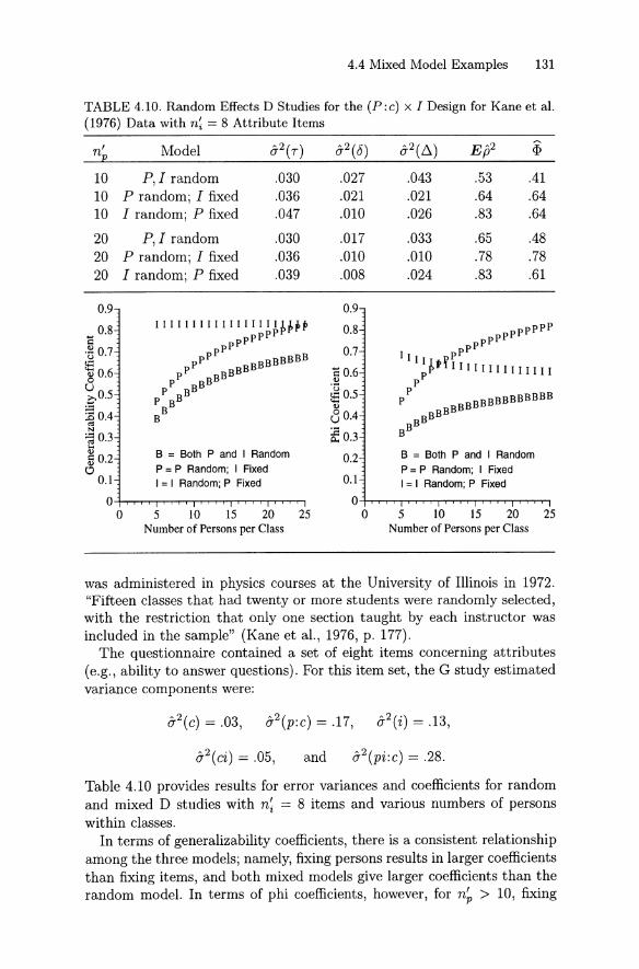
4.4 Mixed Model Examples 131

TABLE 4.10. Random Effects D Studies for the (P :c) x I Design for Kane et al.(1976) Data with n~ = 8 Attribute Items

n' Modelp

10 P,Irand om10 P random; I fixed10 Irandom; P fixed

20 P,Irandom20 P random ; I fixed20 Irandom ; P fixed

.030

.036

.047

.030

.036

.039

.027

.021

.010

.017

.010

.008

.043

.021

.026

.033

.010

.024

.53

.64

.83

.65

.78

.83

.41

.64

.64

.48

.78

.61

5 10 15 20 25Number of Persons per Class

B = Both P and IRandomP = P Random; I FixedI =IRandom; P Fixed

B = Both P and IRandomp = P Random; I FixedI =IRandom; P Fixed

5 10 15 20 25Numberof Persons per Class

0.9

0.8

0.7

C 0.6.,;g 05.... ..,80.4

~0.3

0.2

0.1

o-+-r...........-'T'T'-r--r-r ,...,....,rT""'""'T""T'T"!'"'T""T"'T'T",...,....,....,..,

o

0.9

0.8C'13 0.7t;:

'8 0.6u.q O,5

:E 0.4s:.; 0.3....,&i 0.2o

0.1

o-+-r"T"'T"'T'T'.........,...,....,rT""'""'T""T'T"!'"'T'T'T'T",...,....,....,..,

o

was administe red in physics courses at the University of Illinois in 1972."Fiftee n classes that had twenty or more students were random ly selected,with t he restriction that only one section t aught by each instructor wasincIuded in t he sample" (Kane et al., 1976, p . 177).

The quest ionn aire contained a set of eight items concern ing at tributes(e.g., ability to answer questions). For this item set , the G study est imatedvari ance components were:

and

Table 4.10 provides resul ts for erro r variances and coefficients for randomand mixed D st udies with n~ = 8 items and various numbers of personswithin classes.

In terms of generalizability coefficients, there is a consiste nt relationshipamong t he t hree models; namely, fixing persons results in larger coefficientst han fixing it ems, and bot h mixed models give larger coefficients t han therando m model. In te rms of ph i coefficients , however , for n~ > 10, fixing

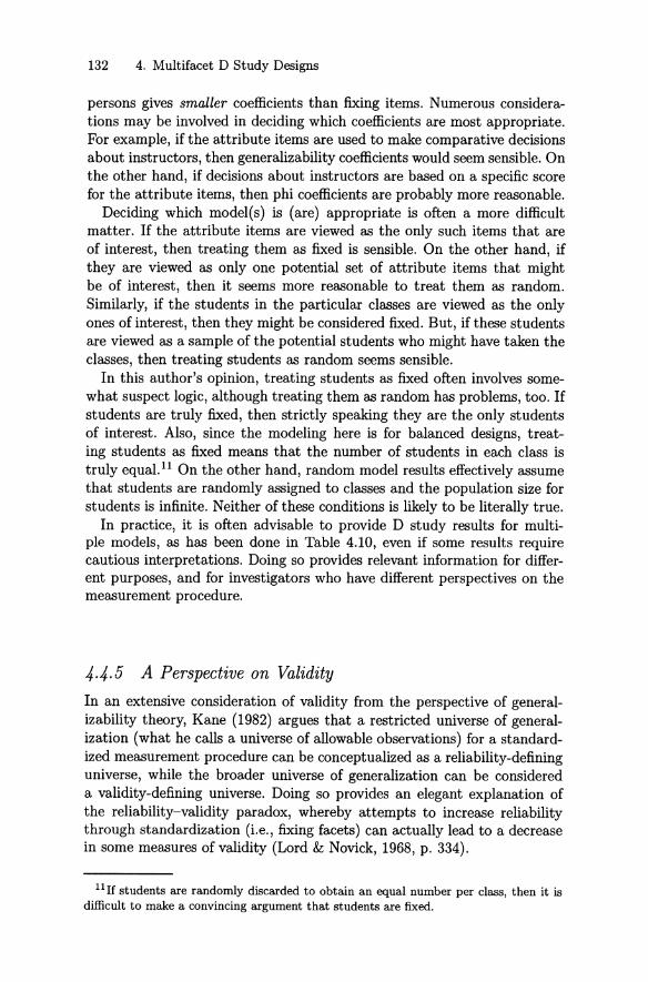
132 4. Multifacet D Study Designs

persons gives smaller coefficients than fixing items. Numerous considera­tions may be involved in deciding which coefficients are most appropriate.For example, if the attribute items are used to make comparative decisionsabout instructors, then generalizability coefficientswould seem sensible. Onthe other hand, if decisions about instructors are based on a specific scorefor the attribute items, then phi coefficients are probably more reasonable.

Deciding which model(s) is (are) appropriate is often a more difficultmatter. If the attribute items are viewed as the only such items that areof interest, then treating them as fixed is sensible. On the other hand, ifthey are viewed as only one potential set of attribute items that mightbe of interest, then it seems more reasonable to treat them as random.8imilarly, if the students in the particular classes are viewed as the onlyones of interest, then they might be considered fixed. But, if these studentsare viewed as a sample of the potential students who might have taken theclasses, then treating students as random seems sensible.

In this author's opinion, treating students as fixed often involves some­what suspect logic, although treating them as random has problems, too. Ifstudents are truly fixed, then strictly speaking they are the only studentsof interest. Also, since the modeling here is for balanced designs, treat­ing students as fixed means that the number of students in each class istruly equal. 11 On the other hand, random model results effectively assurnethat students are randomly assigned to classes and the population size forstudents is infinite. Neither of these conditions is likely to be literally true.

In practice, it is often advisable to provide D study results for multi­ple models, as has been done in Table 4.10, even if some results requirecautious interpretations. Doing so provides relevant information for differ­ent purposes, and for investigators who have different perspectives on themeasurement procedure.

4.4.5 A Perspective on Validity

In an extensive consideration of validity from the perspective of general­izability theory, Kane (1982) argues that a restricted universe of general­ization (what he calls a universe of allowable observations) for a standard­ized measurement procedure can be conceptualized as a reliability-defininguniverse, while the broader universe of generalization can be considereda validity-defining universe. Doing so provides an elegant explanation ofthe reliability-validity paradox, whereby attempts to increase reliabilitythrough standardization (i.e., fixing facets) can actually lead to a decreasein some measures of validity (Lord & Novick, 1968, p. 334).

lllf students are randomly discarded to obtain an equal number per dass, then it isdifficult to make a convincing argument that students are fixed.

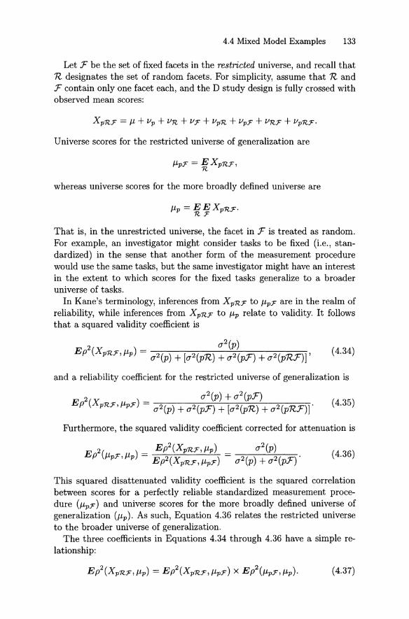
4.4 Mixed Model Examples 133

Let F be the set of fixed facets in the restricted universe, and recall thatn designates the set of random facets. For simplicity, assurne that n andF contain only one facet each, and the D study design is fully crossed withobserved mean scores:

Universe scores for the restricted universe of generalization are

whereas universe scores for the more broadly defined universe are

That is, in the unrestricted universe, the facet in F is treated as random.For example, an investigator might consider tasks to be fixed (i.e., stan­dardized) in the sense that another form of the measurement procedurewould use the same tasks, but the same investigator might have an interestin the extent to which scores for the fixed tasks generalize to a broaderuniverse of tasks.

In Kane's terminology, inferences from XpRF to f.lpF are in the realm ofreliability, while inferences from XpRF to f.lp relate to validity. It followsthat a squared validity coefficient is

(4.34)

and a reliability coefficient for the restricted universe of generalization is

(4.35)

Furthermore, the squared validity coefficient corrected for attenuation is

(4.36)

This squared disattenuated validity coefficient is the squared correlationbetween scores for a perfectly reliable standardized measurement proce­dure (f.lpF) and universe scores for the more broadly defined universe ofgeneralization (f.lp). As such, Equation 4.36 relates the restricted universeto the broader universe of generalization.

The three coefficients in Equations 4.34 through 4.36 have a simple re­lationship:

(4.37)

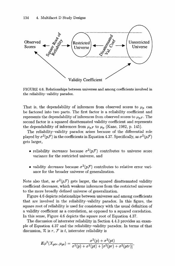
ValidilyCoefficient /

134 4. Multifacet D Study Designs

~Cs'

Observed ~ .:?Scores +-e.~'::.:$~

§~,?o-,~

8j~

+---~~cJ ~~~.

.~ .:::."J'__________'9.____________________ .

FIGURE 4.6. Relationships between universes and amongcoefficients involved inthe reIiability-vaIidity paradox.

That is, the dependability of inferences from observed scores to J,tp eanbe factored into two parts. The first faetor is a reliability coefficient andrepresents the dependability of inferences from observed scores to J,tpF' Theseeond factor is a squared disattenuated validity coefficient and representsthe dependability of inferences from J,tpF to J,tp (Kane, 1982, p. 145).

The reliability-validity paradox arises because of the differential roleplayed by (j2(pF) in the coefficients in Equation 4.37. Specifically, as (j2(pF)gets larger,

• reliability increases because (j2(pF) eontributes to universe scorevariance for the restricted universe, and

• validity decreases beeause (j2(pF) contributes to relative error vari­anee for the broader universe of generalization.

Note also that, as (j2(pF) gets larger , the squared disattenuated validityeoefficient decreases , which weakens inferences from the restricted universeto the more broadly defined universe of generalization.

Figure 4.6 depicts relationships between universes and among coefficientsthat are involved in the reliability-validity paradox. In this figure, thesquare root of reliability is used for consistency with the usual definition ofa validity eoefficient as a correlation, as opposed to a squared correlat ion.In this sense, Figure 4.6 depicts the square root of Equation 4.37.

The discussion of interrater reliability in Section 4.4.3 provides an exam­pIe of Equation 4.37 and the reliability-validity paradox. In terms of thatdiscussion , R. is r , F is t, interrater reliability is

4.5 Summary and Other Issues 135

the squared validity coefficient is

(4.38)

and th e square d disattenuat ed validity coefficient is

(4.39)

So, as (12 (pt) gets larger , interrater reliability will increase, and squaredvalidity as defined by Equation 4.38 will decrease. Also, as (12(pt) getslarger , t he link between the restricted universe and the broader one, asdefined by Equation 4.39, will become weaker. 12

From Kane's perspective on the reliability-validity paradox, it makessense to call Equ ati on 4.38 a squared validity coefficient. Clearly, however,Equation 4.38 is a genera lizability coefficient for a universe of generalizationin which both raters and tas ks are random. This te rminological ambiguityillustrates that generalizability theory "blurs" arbitrary distinctions be­tween reliab ility and validity (Cronbach et al., 1972, p. 380; Brennan , inpress) and forces an invest igator to concent rate on the intended inferences,whatever terms are used to characterize them.

In this discussion of the reliability- validity paradox, it was assumed th atR and :F contain only one facet each. The th eory discussed here has no suchrestriction, however , although equat ions become more complicated when Rand / or :F cont ain multiple facets . Also, it is entirely possible that th e morebroadly defined universe could have one or more fixed facets provid ed th eyare also fixed in the restricted universe. That is, there could be two sets offixed facets: t hose that are fixed in both universes and those that are fixedin the rest ricted universe only.

4.5 Summary and Other Issues

A great deal of the essence of genera lizability theory is capt ured by address­ing one cent ral question, "What const it utes a replication of a measurernentprocedure?" Answering this question requires particular attention to whichfacets are fixed and which are rand om in an investigator-defined rnulti­faceted universe of generalizat ion. Generalizability theory does not provideanswers to question s about which facets should be fixed and which shouldbe randorn. Such answers rnust be sought in the investigator 's substan­t ive theory and intended interpretations. But , generalizability t heory does

12T he squared disattenuated valid ity coefficient in Equ at ion 4.39 is essent ially whatGulliksen (1950 , p. 214) ca lls "conte nt" reliability. It is a lso ca lled "score" reliability insome of t he performan ce assessment literature (see Dunbar et al., 1991).

136 4. Multifacet D Study Designs

provide powerful tools for determining the measurement consequences ofdecisions about which facets are fixed and which are random.

From the perspective of generalizability theory, defining a measurementprocedure requires explicit decisions about three issues:

1. which facets are fixed and which are random in the universe of gen­eralization,

2. D study sample sizes, and

3. D study design structure.

The first issue influences universe score variance , but all three issues in­fluence error variances . In this sense, understanding error variance is amore challenging undertaking than understanding universe score variance.In particular, all three issues need to be taken into account in assessing theinfluence of particular facets on error variance.

In an attempt to simplify interpretations, G study estimated variancecomponents are sometimes converted to percents. For example, for theclass means example in Section 4.4.4, the sum of the estimated variancecomponents is .66, and the percents are given below.

Effect

a2 (a )Percents

c

.034.55

p:c

.1725.76

i

.1319.70

ci

.057.58

pi :c

.2842.42

The virtue of these percents is that they are scale independent. However,they are easily misinterpreted as indicators of the "importance" of eacheffect and/or facet. Such interpretations generaBy require attending to par­ticular statistics, such as error variances, and the kinds of D study issuesmentioned in the previous paragraph. For the class means example, Ta­ble 4.10 clearly indicates that judgments about the contribution of variousfacets to measurement precision depend heavily on such D study issues.

One of the distinct advantages of the procedures discussed in this chap­ter is that they do not require much computational effort once G studyvariance components have been estimated. A hand calculator is often suf­ficient. However, the computer program GENOVA (see Appendix F) canbe used to perform all computations that have been discussed here.

4.6 Exercises

4.1* Assuming effects are uncorrelated, prove the last equality in Equa­tion 4.8; namely,

4.6 Exercises 137

4.2 For the p x I x H design, show that the manner in which score ef­fects are defined in generalizability theory is a sufficient basis for theuncorrelated-effects result (J(VpH , VH) = 0, where the covariance istaken over p and H .

4.3 For the p x (I: H) random effects design, starting with the definitionof (J2(X) in Equation 4.19, show that

2 - (J2(p) (J2(h) (J2(i:h) (J2(ph) (J2(pi:h)(J (X) = -n-'- + - n-'- + n'n' + -n-'-n-'- + -n-'':'::'n-'n-'-'- '

p h t h ph pth

and that Equation 4.20 applies.

4.4* Demonstrate th at it is generally not possible to use the variance com­ponents for a G study p x (i :h) design to est imate results for a Dstudy (I x H) :p design. Show that it is possible to do so if it is as­sumed that (J2( ih:p) = O.

4.5 Consider , again, the p x t x r example in Exercise 3.6.

(a) Provide estimates of D study variance components, universescore variance, error variance, and coefficients for the randommodel with sampie sizes of n~ = 3 and n~ = 2, and with sampiesizes of n~ = 6 and n~ = 1.

(b) For both D studies the total number of observations per personis n~n~ = 6. Why, then, are the error variances for the second Dstudy larger jsmaller th an those for the first?

(c) Estimat e the variance components für the p x i design für theundifferenti ated dat a set with two tasks and three raters, anddetermine Cronbach's alpha for these data.

(d) Why is Cronbach's alpha smallerj larger th an the generalizabilitycoefficient in (a) when n~ = 3 and n~ = 2?

4.6* Consider the G study results in Table 3.4 on page 74 for the randomeffects p x (r :t) design and Synthetic Data Set No. 4. Under a randommodel, what are the D study est imated variance components, universescore variance, error variances and coefficients for the sampie sizes:

(a) n~ = 1 and n~ = 12, and

(b) n~ = 2 and n~ = 6?

Provide box-bar plots , as weil. What is the similarity between theseresults and the corresponding results in Table 4.6 for the p x (R :T)design?

138 4. Multifacet D Study Designs

4.7* Recall the Gillmore et al. (1978) example of the (p:c :t) x i designin Exercise 3.5. Suppose teachers are the objects of measurement.Under random model assumptions, if n~ = 20 and n~ = 11, what ist~minimum number of classes required for the signal-noise ratioSjN(8) to be at least 2?

4.8 For the CAP example in Table 4.7, suppose the task facet were fixedwith n~ = 5 and the rater facet were random with n~ = 1. What arethe estimated universe score variance, error variances, and coefficientsfor the p x T x R design and for the p x (R :T) design? Report resultsto three decimal places. Why are these results so different from thosefor the random model?

4.9* For the random and mixed models in Table 4.8, what is the estimatedstandard error of the mean a(X), assuming n~ = 10, n~ = 3, andn~ = 2?

4.10* Many writing assessments involve exercises or tasks in different genres(e.g., narrative, informational, informative, persuasive, etc.). SupposeG study estimated random effects variance components are availablefor the p x (r: t :g) design, where p stands for students, r stands forraters, t stands for exercises or tasks, and g stands for genre.

(a) Provide a formula for an estimated generalizability coefficientbased on a D study design in which genre is fixed at n~ = 2,there is only one exercise for each genre, and there is only onerating of each exercise.

(b) Suppose data were available for this D study design and Cron­bach's alpha were computed for the four ratings. Estimate alphabased on the G study estimated random effects variance com­ponents.

(c) Why is alpha largerjsmaller than the generalizability coefficientin (a)?

4.11 Assuming items are fixed and persons are random, provide an expres­sion for Eß2 for dass means in terms of mean squares, when G andD study sample sizes are the same.

4.12 In Table 4.10, Eß2 for dass means with items random and personsfixed is nearly constant for all values of n~. Explain this result interms of signal-noise ratios.

4.13 Recall the blood pressure example in Section 2.3.4 from Llabre et al.(1988). In the same paper they describe a study in which each of 40persons had their blood press ure taken in a laboratory using a mer­cury sphygmomanometer. Measurements were taken on two consec­utive days (d), with three replications (r) collected on each day. The

4.6 Exercises 139

resulting G study estimated variance components for the p x (r: d)design were:

Effect

Pdr:dpdpr:d

Systolic83.41

.73

.3024.919.91

Diastolic36.49

oaoa

21.697.99

aSlightly negative estimate replaced by O.

(a) Assuming an investigator wants to generalize over both daysand replications within day, which of these two facets is likelyto contribute more to errors in blood pressure measurements?

(b) Assuming a random model with n~ = 2, what is the minimumnumber of replications required for systolic blood pressure tohave 1> ~ .8? In this case, what is a(~)?

(c) Assuming a random model with n~ = 2, what is the minimumnumber of replications required for diastolic blood pressure tohave <I> ~ .8?

(d) If an investigator does not intend to generalize over days, whatare a(~) and 1> for a single replication, for both systolic anddiastolic blood pressure?

5Advanced Topics in UnivariateGeneralizability Theory

Chapter 3 discussed G studies for random models primarily, although Sec­tion 3.5 provided general procedures for estimating G study variance com­ponents for any model. By contrast, the D study procedures in Chapter 4are based solelyon using random effects G study estimated variance com­ponents. The obvious gap in these discussions is a consideration of generalprocedures for D studies. That is the subject of Section 5.1. Subsequent sec­tions treat stratified objects of measurement , conditional standard errorsof measurement, and several other issues.

5.1 General Procedures for D Studies

The procedures discussed in Chapter 4 are sufficient for estimating D studyresults for most univariate balanced designs in generalizability theory. How­ever, these procedures have severallimitations. First, they presume that Gstudy variance components are estimated for a random model. Sometimes ,however, one or more facets are clearly fixed for the universe of admissibleobservations. Second, for mixed model D studies, the simplified proceduresin Section 4.3 do not provide estimates of the variance components forthe effects in the linear model associated with the D study design and re­stricted universe of generalization, that is, a universe of generalization inwhich one or more facets is fixed. In this sense, these procedures are suscep­tible to misunderstanding. Third, the procedures discussed in Chapter 4 donot apply to D study designs that involve sampling from a finite universe.

142 5. Advanced Topics

Such designs are not common in generalizability t heory, but they do occuroccasionally.

Some additional not ation al conventions are required to accommodatedist inctions drawn in this sect ion. First , we use N' to designate t he sizeof a facet in the universe of generalization. Second , we use a2 (ä IM ' ) todesignate D st udy variance components for mean scores for a model M 'that relat es the D st udy design and the universe of generalization. Recallthat a 2 (a IM ) was introduced in Section 3.5 to designat e G st udy variancecomponents for a model M. Throughout this sect ion -r designates the ob­jects of measurement , N~ --+ 00 , and it is assumed that r is not nest edwithin any other facet.

5.1.1 D Study Variance Components

Before considering a general equat ion for obtaining a 2 (äIM') from a 2 (alM),two special cases are considered: (a) for each facet N' = N , which may ormay not approach infinity; and (b) for each facet N' ::::; N --+ 00 . Unlessot herwise noted , it is assumed in thi s section that the G and D st udy havet he same design structure.

N' = N for Each Facet

In t his case, t he universe of generalizat ion and t he universe of admissibleobservations are the same size, and

where a 2 (a IM ) is discussed in Section 3.5,

{

1 if ä = r , and, otherwise, the productd(ä lr) = ofthe D st udy sample sizes (n') for all

indices in ä except r ,

and

{

t he product of the terms (1 - n' IN')C(älr) = for all primary indices in ä except r

[C(älr ) = 1 if ä = r].

(5.1)

(5.2)

(5.3)

Recall that a prim ary index is one that appears before any colon in t henotational representation of a component.

T he term C(ä lr ) is a finite universe correction factor (see, e.g., Cochran,1977, pp . 23-25) . When N ' --+ 00 , C(älr) = 1 and Equation 5.1 becomest he familiar equation for a random effects D study est imated variance com­ponent. If n' = N' for any primary index in ä, t hen C(älr) = 0 anda 2 (ä IM ' ) = O.

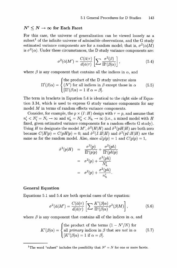
5.1 General Procedures for D Studies 143

N' ::; N -t 00 for Each Facet

For this case, the universe of generalization can be viewed loosely as asubset ' of the infinite universe of admissible observations, and the G studyestimated varian ce components are for a random model; that is, (1'2(aIM)is (1'2(a) . Under these circumstances, the D study variance components are:

2 _ , C(äIT) [", (1'2(ß) ](1' (alM) = d(äIT) ~ TI'(ßla) ,

where ß is any component th at contains all the indices in o, and

{

the product of the D study universe sizesTI'(ßla) = (N') for all indices in ß except those in a

[TI'(ßla) = 1 if a = ß].

(5.4)

(5.5)

The term in brackets in Equat ion 5.4 is identical to the right side of Equa­tion 3.34, which is used to express G study variance components for anymodel M in terms of random effects variance components.

Consider , for example, the P x (1 :H) design with T = p, and assurne thatn~ < NI = Ni -; 00 and n~ = Nh< Nh -; 00 (i.e., a mixed model with Hfixed, given est imated variance components for a random effects G study) .Using H to designate the model M' , a-2(H IH ) and a-2 (pH IH ) are both zerobecause C(Hlp) = C(pHlp) = 0; and a-2(I :H IH ) and a-2(p/ :H IH ) are thesame as for the random model. Also, since C;(plp) = 1 and C(plp) = 1,

(1'2(p) (1'2(ph)--=--'-+--=---'--TI' (plp) TI' (phlp)

2 ( ) (1'2(ph)(1' P+~

h

2() (1'2(ph)(1' P + --,-.n h

General Equation

Equations 5.1 and 5.4 are both special cases of the equation:

2(-IM') = C(äIT) [", K'( ßla) 2(ßIM )] (5.6)(1' a d(äIT) ~ TI'(ßla) (1' ,

where ß is any component th at contains all of the indices in a, and

{

the product of the terms (1 - N' IN) forK'( ßla) = all primary indices in ß that are not in a

[K'(ßla) = 1 if a = ß] .(5.7)

IThe word "subset" includes the possibility th at N' = N for one or more facets .

144 5. Advanced Topics

Equation 5.6 applies under the very general condition that n' :s N ' :s Nfor each facet , where N may or may not approach infinity.

5.1.2 Universe Score Variance and Error Variances

Let

{the set of all random facets in the universeof generalization such that n' < N ',

{the set of all fixed facets (i.e., n' = N' ) inthe universe of generalizat ion,

{

an observable mean score for an objectof measurement r , which is also denotedXr'RF , and

{t he average value of X r over all sampledobjects of measurement.

Note that in this section, a facet occurs in R if conditions of t he facet aresampled from a larger , but possibly finite, set of condit ions.

By definition , the universe score associated with an object of measure­ment is

(5.8)

Note that, since an observed mean score involves all levels of a ll fixed facet sF , universe score does not involve taking an expectat ion over any of them.Absolute error is

(5.9)

relative error is(5.10)

and the error associated with using X as an estimate of /L is simply X - /L.To identify which score effects ente r /Ln ß n and 8r , the observable quan­

tities X rand X can be replaced by their expressions in terms of scoreeffects. Then the variances of /Ln ß n and 8r can be obt ained algebraically.These variances will involve the a2(äIM') , as provided by Equations 5.1,5.4, or 5.6. This tedious process can be circumvented using the followingrules.

Rule 5.1.1: a2(T) is the part icular a2(ä IM' ) with ä = T,

Rule 5.1.2: a2 (ß ) is the sum of all the a2 (ä IM' ) except a2(rJM') , and

Rule 5.1.3: a2 (8) is the sum of all the a2 (ä IM' ) such that ä includesr and at least one of the indices in R .

5.1 General Procedures for D Studies 145

TABLE 5.1. D Studies for the APL p x (I :H) Design for the Southern Region

D Studies

n' 5 5hO'2(a IH ) n' 8 20,

O'2(pIH ) = .0378 O'2(pIH ) .0378 .0378O'2(hIH ) = .0013a O'2(H IH )

O'2(i :hIH ) = .0259 O'2(I :H IH ) .0006 .0003O'2(phIH ) = .0051 O'2(pH IH )

O'2(pi :hIH ) = .1589 O'2(pI :H IH ) .0040 .0016

0'2(7) .0378 .0378O'2(0) .0040 .0016

O'2(~) .0046 .0019Eß2 .905 .959

1> .892 .952aStrictly sp eaking, a-2 (hIH ) is a quadrat ic form .

These rules, which bear an obvious similarity tp those for the randommodel , rely heavily on the fact that a2 (ä IM ' ) = 0 when n' = N' for aprimary index in ä (except 7). Given these rules, the usual formulas applyfor a2(X ), E p2 , and <I> (see Table 4.3 on page 109), as weIl as for signal­noise and error- tolerance ratios.

5.1.3 Examples

The procedures discussed in Sections 5.1.1 and 5.1.2 are general enough toapply to virtually all D studies for balanced designs, although the simpli­fied procedures in Chapter 4 are often sufficient . Th e examples consideredhere are illustrative of situ ations in which the simplified procedures do notsuffice.

APL Survey with N' = N for each Facet

Table 3.7 on page 91 reported variance components for the APL Surveydiscussed in Section 3.5. These variance components are for a p x (i :h)design under a mixed model in which n i = 8 items are nested withineach of nh = Ni, = 5 fixed content categories. Table 5.1 reports D studyresults for the same mixed model; that is, nh = Nft = Ni, = 5 and n~ <NI = Ni --+ 00 . Both the G and D study perspectives on this exampleassurne that the measurement procedure would always involve the sameset of fixed categories, which means that generalization is intended oversampies of items (within content areas) only.

Clearly, for thi s example, 7 = P because persons are the objects of mea­surement. Since H is fixed, we designate the model simply as H . The D

146 5. Advanced Topics

study estimated variance components a-2(äIH) are obtained using Equa­tion 5.1 since N' = N for both facets. For example, for a-2(I :HIH) anda-2(pI:HIH), d(älp) = n~n~ , and C(älp) = 1 because NI -. 00 . Therefore,

a-2(I:HIH) = a-2(i,:h)H)

and a-2(pI:HIH) = a-2(p; :~IH) .~~ ~~

For both a-2(HIH) and a-2(pHIH), C(älp) =°because n~ = Nh. There­fore, both a-2(HIH) and a-2(pHIH) are zero. To appreciate why these twovariance components disappear, recall the notion of replications of a mea­surement procedure. For this example , each replication yields person meanscores over samples of n~ items from every one of the five content areas.Therefore, the set of content area means is constant for all replications.Effectively, this implies that J.LH gets absorbed into J.L and J.LpH gets ab­sorbed into J.Lp . It follows that I/H = J.LH - J.L = 0, which necessarily leadsto a2(H IH ) being zero. Also,

I/pH = (J.LpH - J.Lp) - (J.LH - J.L) =°-°= 0,

which necessarily leads to a2(pH IH ) being zero.In short, because generalization is over only one facet (items) , there are

only three nonzero variance components for the D study p x (I: H) designwith H fixed. This is directly analogous to the fact that there are threevariance components for the D study p x I design and its single-faceteduniverse of generalization.

It is important to note that the procedures employed in this examplerely heavily on the fact that an equal number of items are nested withineach content category. If that were not the case, then the design would beunbalanced and best treated using the multivariate generalizability theoryprocedures discussed in Chapters 9 and 11.2

Mixed Model D Study Given G Study Random Effects VarianceComponents

Using G study random effects variance components, Section 4.3 consideredsimplified procedures for obtaining mixed-model D study results. One ofthe examples involved the p x (R :T) design for Synthetic Data Set No. 4 inTable 3.2, under the assumption that an investigator wanted to generalizeto a restricted universe of generalization with tasks fixed at n~ = NI = 3.In considering this example, it was pointed out that the random effectsestimated variance components a-2 (0:) in Table 4.8 are not associated withthe restricted universe of generalization, even though they can be used toobtain unbiased estimates of universe score variance , error variances , andcoefficients for the restricted universe.

2The APL example considered here is a very simple vers ion of the tabl e of sp ecifica­tions model outlined later in Section 9.1.

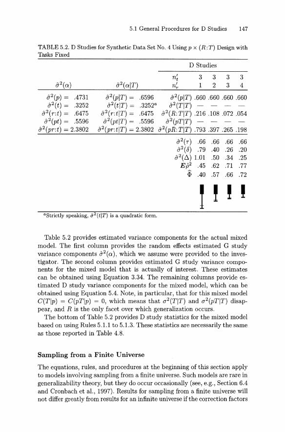
5.1 General Procedures for D Studies 147

TABLE 5.2. D Studies for Synthetic Data Set No. 4 Using p x (R :T) Design withTasks Fixed

D Studies

a2 (p) = .4731a2 (t ) = .3252

a2(r :t ) = .6475a2 (pt ) = .5596

a2(pr :t ) = 2.3802

a2(pIT ) = .6596a2 (t IT ) = .3252 a

a2(r :t IT ) = .6475a2(pt IT ) = .5596

a2(pr :t IT ) = 2.3802

n~ 3 3 3 3n~ 1 2 3 4

a2(pIT ) .660 .660 .660 .660a2(T IT ) - - - ­

a2(R:TIT) .216 .108 .072 .054a2(pT IT ) - - - ­

a2(pR:T IT ) .793 .397 .265 .198

a2(T) .66 .66 .66 .66172(8) .79 .40 .26 .20a2(~) 1.01 .50 .34 .25

E ß2 .45 .62 .71 .77~ .40 .57 .66 .72

aSt rictly speaking, a-2 (t IT ) is a quadratic form.

Table 5.2 provides estim ated variance components for the act ual mixedmodel. The first column provides the random effects estimated G studyvariance components 172(0: ), which we assurne were provided to the inves­tigator. The second column provides est imated G study variance compo­nents for the mixed model that is act ually of interest. These est imatescan be obtained using Equation 3.34. The remaining columns provide es­t imat ed D study vari ance components for the mixed model, which can beobtained using Equation 5.4. Note, in particular , that for this mixed modelC(Tlp) = C(pTlp) = 0, which means that (T2(TIT) and (T2(pTIT) disap­pear , and R is th e only facet over which generalizat ion occurs .

The bottom of Table 5.2 provides D study statistics for the mixed modelbased on using Rules 5.1.1 to 5.1.3. These st ati stics are necessarily the sameas those reported in Table 4.8.

Sampling from a Finite Universe

The equations, rules, and procedures at the beginnin g of this section applyto models involving sampling from a finite universe. Such models are rare ingeneralizability theory, but they do occur occasionally (see, e.g., Section 6.4and Cronb ach et al. , 1997). Results for sampling from a finite universe willnot differ greatly from results for an infinite universe if the correction factors

148 5. AdvancedTopics

TABLE 5.3. D Studies for Synthetic Data Set No. 4 Using the p x (R :T) Designfor Sampling n~ = 2 Tasks from a Finite Universe of Nt = N: = 3 Tasks

D Study

0-2 (pi Nt = 3) = .6596a-2(tlNt = 3) = .3252

a-2(r:tINt = 3) = .6475a-2(ptlNt = 3) = .5596

a-2(pr :tINt = 3) = 2.3802

a-2(öINI = 3) ford(ölp) O(ölp) n~ = 2 and n~ = 6

1 1 a-2(pINI = 3) = .6602 1/3 a-:l(TINI = 3) = .05412 1 a-2(R: TINI = 3) = .0542 1/3 a-2(pTINI = 3) = .09312 1 a-2(pR :TINI = 3) = .198

a-2(7) = .66a-2(0) = .29

a-2(ß) = .40Eß2 = .69

<P = .62

0(öI7) are elose to one. When correction factors are considerably smallerthan one, however, differences can be important.

Consider, again, the p x (R:T) design and Synthetic Data Set No. 4under the assumptions that:

1. each replication of the D study design involves sampling n~ = 2 tasksfrom a finite facet of size NI = 3, and

2. each of the two tasks is evaluated by a random sample of n~ = 6raters from a facet of infinite size.

Presumably, the NI = 3 tasks in the universe of generalization are theactual nt = 3 tasks in the G study,"

Under these assumptions, Table 5.3 provides both G and D study re­sults." The first column in Table 5.3 provides the G study estimated vari­ance components for Nt = 3, which are identified as a-2(aINt = 3). Theycan be obtained using Equation 3.34. These estimates are necessarily identi­cal to the a-2(aIH) in Table 5.2, because the facet sizes (N) for the universe(of admissible observation) are the same for both sets of estimates.

The last column in Table 5.3 provides estimates of the D study variancecomponents. Note , in particular, that a-2(TINI = 3) and a-2(pTINI = 3)are both nonzero because their correct ion factors are nonzero. None of theestimated variance components disappear because sampling is involved for

3If this were not true, interpretations would be strained, at best.4The G study randorn effects est irnate d variance cornpon ents are , of course, the same

as those in Table 5.2.

5.1 General Procedures für D Studies 149

both facets in the universe of generalization, even th ough one of these facets(tasks) is of finite size.

It is instructive to compare D study statistics for sampling from a finiteuniverse in Table 5.3 with the corresponding results for the random modeland the mixed model. With n~ = 6 randomly selected raters, and withn~ = 2, these results are as foIlows.

Model

Random (N: -> (0)Finite sampling (N: = 3)Mixed (N: = 2)

.47

.66

.75

.48

.29

.20

.69

.40

.25

.95

.95

.95

The pattern of t hese results is predict able based solelyon the size of N: :

• universe score variance increases as the size of the universe of gener­alizat ion decreases,

• error variances decrease as the size of the universe of generalizationdecreases , and

• expected observed score vari ance is unaffected by the size of the uni­verse of generalizat ion.

5.1.4 Hidd en Facets

Any reasonably complete discussion of generalizability theory distinguishesbetween universes of admissible observations and universes of generaliza­tion, as weIl as between G studies and D studies. Yet , it is evident thatsome applicat ions of the theory do not require sharp distinctions amongaIl four concepts. For example, when only one set of data is available andthere is no intent to speculate about generalizability for different samplesizes, it can be awkward to talk about two studies, The role of "hidden"facets in generaliz abili ty theory, however , makes important use of aIl fourconcepts.

EssentiaIly, a facet is hidden when there is only one sampled condit ion ofthe facet , which induces interpret ational complexiti es and (usuaIly) bias instatistics such as E p2. It is important to understand that generalizabilitytheory does not create these complexit ies; rather it helps an investigatorunderstand these complexit ies, isolat e sour ces of bias , and even est imatethem. These matters are illustrated next using examples of a hidd en fixedfacet and a hidden random facet.

Hidden Fixed Facets and Internal Consistency Coefficients

A coefficient of int ern al consistency such as Cronbach's (1951) alpha orKuder and Richardson's (1937) Formul a 20 is typic aIly obtained using data

150 5. Advanced Topics

TABLE 5.4. Two Perspectives on the p x I Design

D Studies: n~ = 1 and n~ = 4

a2 (p) = .5528a2 (i ) = .4417a2(0) = .0074a2 (pi ) = .5750a2(po) = .1009a2 (io) = .1565

a2 (pio) = .1565

a2 (plo) = .6537a2 (i lo) = .5982

a2(plo) = .654a2 (110) = .150

a2(7) = .65a2 (8) = .38

Eß2 = .63

a2 (p) = .553a2 (1) = .110a2(0) = .007

a2 (p1) = .144a2 (po) = .101a2 (10) = .039

a2 (p10) = .234

a2(7) = .55a2

( 8) = .48E ß2 = .54

collected on a single occasion, although users often interpret such resultsas if they generalize to other occasions. Let us consider thi s situation fromthe perspective of generalizability theory.

Specifically, recall Synthetic Data Set No. 3 for the p x i x 0 design inTable 3.1 on page 72, which has four items administered on two occasions.The first column in Table 5.4 reports the G study random effects est imatedvariance components . The last column reports the D study estimated vari­ance components and typical statistics for the random model, under theassumpt ions that n~ = 4 and a single occasion is randomly sampled from auniverse of occasions. Let us cont rast these results with those for a singlefixed occasion.

The second column in Table 5.4 provides G study estimated variancecomponents for No = 1, which can be obtained from the random effectsvariance components in the first column using Equation 3.34:

a2 (plo)

a2 (i lo)

a2 (pi lo)

a2 (p) + a2 (po)

= a2 (i ) + a2 (io)

a2 (pi ) + a2(pio).

(5.11)

(5.12)

The third column provides D study estimated variance components forN~ = 1, which can be obt ained using Equation 5.4 or, more simply, bydividing Equations 5.11 and 5.12 by n~ = 4. Note that , by comparison withthe random model results, for a single fixed occasion,

• error variances are smaller, and

• universe score variance and coefficients are larger.

Often, of course, dat a are not collected on two occasions, and reliabilityis estimated simply by computi ng KR-20 or Cronbach's alpha. The result s

5.1 General Procedures for D Studies 151

in Table 5.4 illustrate t hat if generalizat ion is intended over occas ions,then such coefficients will overestimate reliability. T his conclusion directlycontradicts t he conventio nal wisdom that Cronbach's alpha is a lower limitto reliability l''

The lower-limit argument is promulgated, for example, by Lord andNovick (1968) in t heir sect ion on "Coefficient a and t he Reliability of Com­posit e Measurements." As discussed by Brennan (in press), the problemwith t he Lord and Novick proof and all ot hers like it is not t hat t hereis a mathematical error; rather , t he problem is that such proofs fail todifferent iate between t he universe of generalizat ion t hat is of interest toan investigator and the characterist ics of available data. In partic ular, ifdata are collecte d on a single occasion, an est imate of reliability based onsuch data will almost certainly overesti mate reliability when interest is ingenera lizing over occas ions.

When only one condit ion of a facet is sampled, that facet is hidden fromthe investigator in the sense t hat variance components associate d with thatfacet are confounded with other variance components . If all observat ionsare influenced by t he same level of t he facet , then analyses of the data willeffectively treat t he facet as fixed with n = n' = N = N ' = 1. T hat is whywe often refer to occasion as a hidden fixed facet when Cronbach's alphais computed. However, a hidden facet is not always fixed.

Hidden Random Facets and Performance Assessments

Sup pose, for example, that each st udent (P) at a piano recital played a mu­sical select ion (m) of his or her own choosing, with all students evaluated byt he same two judges (j) . Since each st udent played only one musical piece,t he m facet is hidden. Importantly, however , st udents were not required toplay the same musical select ion and, therefore, m is not fixed. Rather , mis more reasonably considered random. To keep matters simple we assumethat each st udent played a different musical selection, and the universe ofgeneralization has musical select ions crossed with judges; t hat is, in t heory,each judge could evaluate performance for each musical selection.

For t his universe of generalizat ion with sampie sizes of n~ = nm = 1and nj = nj = 2, the generalizability coefficient for t he ra ndom effects Dst udy p x m x J design is

(5.13)

P resumably, it is t his coefficient that an investigator would like to est imate.

5There are certainly cases in which alpha is properly interpreted as a lower limit toreliability. Recall, for example, Exercise 4.10.

152 5. Advanced Topics

However, the recital has students (p) completely confounded with musicalselections (m). Therefore, the p x j design that characterizes the availabledata can be denoted more explicitly (p,m) x j, where the notation (p,m)signifies that p and mare completely confounded. This means that

where variance components to the right are for the p x m x j design. Sim­ilarly,

a2[(p, m)j] = a2(pj) + a2(jm) + a2(pjm) .

It follows that E p2 for the (p, m) x J design that characterizes the availabledata is actually an estimate of

E 2 -P2 -

=

a2(p,m) + [a2[(p~m)j]]

a2(p) + a2(m) + a2(pm)

a2(p) + a2(m) + a2(pm) + [a2(pj)

+ a2(jm)

+ a2(pjm)] .

2 2 2

(5.14)

Equation 5.13, with the subscript 1, designates the conceptualization forthe intended universe of generalization. Equation 5.14, with the subscript2, designates the statistic that is estimated using available data. Clearly,Equation 5.14 is not associated with the intended universe of generalization.It is evident from these equations that ar(r) :::; a~(r) , but this does notguarantee that E pr :::; E p~ . However, if

a2(jm) s 2 a2(pm),

then ar(o) 2': a~(o) and EpI :::; Ep~. Conversely, if

a2(jm) » a2(m) + a2(pm),

(5.15)

then it can be true that EpI > Ep~ .6

Clearly, when the m facet is hidden but random, the bias in Ep~ usingthe (p,m) x J design can be either positive or negative, based largely on themagnitude of a2 (jm ). This variance component reflects the extent to whichjudges rank order the difficulty of the musical selections differently. Withwell-trained judges, it seems unlikely that a2(jm) would be very large,and the condition in Equation 5.15 is likely to be true. If so, Ep~ usingthe (p,m) x J design will be an upper limit to reliability for the intendeduniverse of generalization.

6The symbol» means "very much bigger than."

5.2 Stratified Obj ects of Measurernent 153

T his "musical selection" example reasonably weil reflects some of the im­portant considerat ions involved in assessing th e reliability of some types ofperformance assessments , including portfolio assessments, th at have a hid­den random facet. It is particularly important to note th at a hidden randomfacet indu ces bias different from th at induced by a hidden fixed facet , andthe magnitude (and somet imes the direction ) of such bias cannot be ascer­t ained from an analysis of data in which th e facet is hidden. When decisionsare to be made based on n' = 1 for some facet , a G study with n > 1 forth at facet is extraordinarily useful, and often essent ial, because it permitsdisent angling sources of variance th at are otherwise indistinguishable inanalyses of the data with n' = 1.

The "musical selection" example can be extended further by hypothesiz­ing a hidden occasion facet. That is, suppose generalization is intended overoccasions, but th e data used to estimate E p2 come from only one recital.Then, th ere are two hidden facets th at influence th e magnitude E ß2;

1. th e hidden occasion facet that is fixed , which likely causes E ß2 to behigher than it should be; and

2. the hidden musical-selection facet that is randorn , which can causeE ß2 to be either higher or lower than it should be.

Clearly, for this example, a G study with nm > 1 and n o > 1 wouldbe ext raordinarily useful in that it would permit est imat ing th e variancecomponents required for an est imate of reliability for th e intended universeof generalizat ion. This thought experiment indicat es how genera lizabilityth eory helps an investigator understand the consequences of hidden facetson characteristics of a measurement procedure.

Serious considerat ion of many, if not most, real-world studies revealshidden facets. Adesire for simplicity may lead investigat ors to disregardsuch facets, but doing so can lead to misleading interpretations .

5.2 Stratified Objects of Measurement

Often , object s of measurement are st rat ified with respect to some othervariable, and an investigator may be interested in variability within levelsof the stratificat ion variable as weil as variability across levels. To discussand illustrate these matters, consider, again, t he APL Survey. Previousresults (see Tables 3.7 on page 91 and 5.1 on page 145) have focused ononly one region of th e country (south) . Table 5.5 provides results for 608persons in each of four regions (northeast , north cent ral, south, and west)as weil as a "global" analysis for th e undifferentiat ed group of 2432 personsin all regions r+ . We assurne here that regions (r) are fixed and, as before,conte nt catego ries (h) are fixed.

154 5. Advanced Topics

TABLE 5.5. APL Survey Variance Components for All Four Regions

Effect rl r2 T3 r4 r+

p .0446 .0418 .0378 .0403 .0425h .0024 .0024 .0013 .0037 .0024i :h .0272 .0244 .0259 .0203 .0242ph .0056 .0048 .0051 .0050 .0051pi:h .1597 .1431 .1589 .1383 .1503

X .6130 .6886 .6520 .7117 .6663

Tl r2 r3 T4 r+

.0446 .0418 .0378 .0403 .0425

.0007 .0006 .0006 .0005 .0006

.0040 .0036 .0040 .0035 .0038

0'2(7) .0446 .0418 .0378 .0403 .04250'2(0) .0040 .0036 .0040 .0035 .0038O'2(~) .0047 .0042 .0046 .0040 .0044

Xpoih J.t

+vr

+ Vp-r

+Vh

+ vi:h+ Vrh.

+ Vri:h

+ Vph:r

+ Vpi :rh

FIGDRE 5.1. Representations of (p :r) x (i:h) design.

TABLE 5.6. APL Survey Variance Components for (p :r) x (i :h) Design

D Study (72(äIRH)

Eifect

rp:rhi:hrhri :hph :rpi:rh

MB

45.41251.7954

106.022258.9846

.4078

.3609

.1910

.1500

.0018

.0411

.0024

.0242

.0000

.0003

.0051

.1500

Est. Cornfield and Tukey Definitions

.0018 (72(rIRH) = I:r v;/(nr -1)

.0411 (72(p:rIRH) = I:r(Ev;:r)/nr

.0006 (72(1 :HIRH) = EVY:H

.0000 (72(r1:HIRH) = I:r(Ev;I:H)/(nr -1)

5.2 Stratified Objects of Measurement 155

Analyses like those in Table 5.5 are quite adequate for many purposes,but they do not explicitly provide estimated variance components for theactual stratified design (p :r ) x (i :h). A Venn diagram for this design isprovided in Figure 5.1, and the est imated variance components for theAPL Survey are given in Table 5.6.

5.2.1 Relationships Among Variance Components

When nr = N r , nh = Nh , Np --+ 00 , and Ni --+ 00 , we denote the averagevariance components for the individual p x (i :h) designs as

Th ere are simple relationships between these average variance componentsand variance components for the (p:r) x (i :h) stratified design (J"2(aIRH) .Specifically, letting f r = tn; - l) /nr ,

0';(pIH)

O';(hIH)

O';(i:hIH)

0';(phIH)

O';(pi :hIH)

(J"2(p:rIRH)

(J"2(hIRH) + f r(J"2(rhIRH)

= (J"2(i :hIRH) + f r(J"2( ri :hIRH)

(J"2(ph:rIRH)

(J"2(pi: rhIRH) .

(5.16)

It is important to note th at the (J"2(aIRH) are defined in terms of theCornfield and Tukey (1956) conventions (see Section 3.5).

There a re relatively simple formulas for relating variance com pone nts forthe global p x (i :h) design over all regions (J"~(aIH) and variance compo­nents for the (p :r) x (i: h) st rat ified design:

(J"~(pIH)

(J"~(hIH)

(J"~( i :hIH)

(J"~(phIH)

(J"~(pi :hIH)

(J"2(p: rIRH) + f r(J"2(rIRH)(J"2(hIRH)

(J"2( i :hIRH)

(J"2(ph:rIRH) + f r(J"2(rhIRH)

(J"2(pi :rhIRH) + f r(J"2(ri :hIRH) .

(5.17)

For example, the variance component for persons over all regions (J"~ (pIH)involves the variance component for persons within regions (J"2(p:rIRH)and th e variance of the region means (J"2(rIRH) .

Note that (J"2(rIRH) = 2:: v; / (nr - 1) is not involved in Equation Set 5.16but is involved in Equation Set 5.17. Averaging variance components for theindividual regions does not involve variability of the region means, whereasvariance components for r., do involve variability in the region means.

156 5. Advanced Topics

The (1~ (aIH) in Equation Set 5.17 can be used to obtain estimates ofuniverse score variance and error variances for persons over all regions. Todo so,

• use Equation Set 5.17 with Equation 5.1 to obtain D study estimatedvariance components, and then

• use Rules 5.1.1 to 5.1.3 to obtain 8"2(7), 8"2(~) , and 8"2(8) .

The resulting estimates assume the parameters are defined as folIows :

(5.18)

(5.19)

(5.20)

For the (p:r) x (I :H) design and the APL example,

8"2(7)

8"2(~)

8"2(8)

fr8"2(rIRH) +8"2(p:rIRH) = .0425 (5.21)

8"2(I:HIRH) + fr8"2(rI:HIRH) + 8"2(pI:rHIRH) = .0044

= fr8"2(rI :HIRH) + 8"2(pI:rHIRH) = .0038.

These results are virtually identical to those for the global analysis (r+)reported in the last column of Table 5.5. Such equalities are likely whenevernp is large.

Rules suggested by Cardinet et al. (1981) and summarized by Brennan(1992a, pp . 92-97) also could be used to estimate (12(7), (12(8), and (12(~)

for all persons over all regions (see, also, Brennan, 1994). Their rules arequite general in that they permit multiple "inst rumentat ion" facets, whichare associated with the universe of generalization (e.g., items and contentareas) , and multiple "differentiation" facets, which are associated with thepopulation of objects of measurement (e.g., persons and regions). How­ever, their rules do not use the Cornfield and 'Iukey definitions of variancecomponents.

5.2.2 Comments

The subject of stratified objects of measurement illustrates rather dra­matically the importance of giving careful attention to definitions of vari­ance components and D study quantities such as (12(7), (12(~), and (12(8).Clearly, for example, Equation 5.21 for 8"2(7) for the APL example dependson defining variance components according to the Cornfield and Tukey con­ventions and defining (12(7) according to Equation 5.18.

5.3 Conventional Wisdom About Group Means 157

If regions were random, the Cornfield and Tukey definitions imply thatthe multiplicative factor Irno longer applies or , stated differently, Ir shouldbe set to unity. Obviously, this somewhat simplifies the relationships amongvariance components discussed in Section 5.2.1. Otherwise, however, therules and relationships still apply when regions are random.

Sometimes variance components for a stratified analysis are available , butresults for the individual strata are not. In this case, D study results for arandomly sampled stratum can be obtained using the variance componentsthat do not contain the strata index in a primary position. For example,for the APL Survey, the a-2 (a IRH ) that do not contain r as a primaryindex are those for p:r, h , i :h, ph:r , and pi:rh in Table 5.6. These variancecomponents can be used with the rules and pro cedures in Section 5.1 (seeExercise 5.6) .

Throughout this section it has been assumed that the design is balancedin two senses-an equa l number of items within categories and an equalnumber of persons within regions. If either of these condit ions is not ful­filled, then the design is unbalanced , the pro cedures discussed here do notapply, and appropriate pro cedures are much more complicated.

5.3 Conventional Wisdom About Group Means

Sometimes it is asserted that if a test is not reliable enough for makingdecisions about individuals, or if error variance for individuals is unaccept­ably large, then t est scores can still be used for making decisions aboutgroups. Implicit in such a st atement is an assumption that reliability forgroups is necessaril y larger than reliability for persons, and/or error vari­ance for groups is necessarily smaller th an error vari ance for persons. Bren­nan (1995a) , shows that this "convent ional wisdom" about group means isnot necessaril y true. These results are summarized here.

5.3.1 Two Random Facets

Consider the random effects (p:g) x i design with persons (p) nest ed withingroups (g) and crossed with items (i). Suppose that groups are the objectsof measurement, and t he universe of genera lizat ion has P x I , wit h bothfacets being random. For this design and universe, as discussed in Sec­t ion 4.4.4 , the generalizability of group rneans is

(5.22)

158 5. Advanced Topics

By cont ras t , if persons within a single randomly selected group are t heobjects of measurement,

E 2 (J"2(p:g)Pp:g = (J"2(p:g) + (J"2(pI :g) '

and if persons over groups are the objects of measurement,

(5.23)

(5.24)

Usually, when comparative statements are made about reliability coeffi­cients for groups and persons, the intended int erpret at ion of reliability forpersons is given by Equat ion 5.24. Therefore, the convent ional wisdom isviolated when Ep~ < Ep~. It is immediately obvious that this inequalityis true under the trivial (although unlikely) conditions that (J" 2(g) = 0 orn~ -t 00 . Also , Brennan (1995a) shows that this inequ ality is sat isfied when

(J"2 (g) (J"2 (gi)(J"2(g) + (J"2(p:g) < (J"2(gi ) + (J"2(pi:g)'

(5.25)

That is, Inequ ality 5.25 is a sufficient condition for the convent iona l wisdomto be violated.

As an example, refer again to the Kane et al. (1976) course-evaluat ion­questionnaire study discussed in Section 4.4.4. Recall t hat for t he at t ributeitems, the G study est imated vari ance components were:7

0-2(gi) = .05

Using Inequality 5.25,

and

0-2(g) = .03 = 150 < 0-2(gi) = .05 = 1520-2 (g) + 0-2 (p:g) .20 ' 0-2 (gi) + 0-2(pi:g) .33 . .

Therefore, the sufficient condit ion is sat isfied, and E P~ < E P~ for all pairsof values of np and n i. For example, if n~ = 20 and n~ = 8,

Eß~ = .65 < Eß; = .83.

Inequ ality 5.25 is a sufficient condit ion for t he convent ional wisdom aboutreliability coefficients to be violated , but it is not a necessary condit ion .That is, there are circumstances that lead to Ep~ < Ep~ even when In­equality 5.25 is not sat isfied (see Exercise 5.7).

7Here group (g) is used inst ead of d ass (c).

5.4 Conditional Standard Errors of Measurement 159

The conventional wisdom also suggests th at error varian ce for groups isless than error variance for persons . However, this convent ional wisdom isnot necessarily true, either . Relative error variance for group means is:

(5.26)

and relative error variance for person means over groups is:

(5.27)

The conventional wisdom is violated when 0'2(89 ) > O'2(8p). It can beshown (see Exercise 5.8) th at a necessary condition for this inequality is

2 n-1Epp:g >~.

p(5.28)

Clearly, when n p --+ 00 , Inequality 5.28 will not hold. So, for large values ofn p , it is reasonable to assurne th at relative error variance for persons is likelyto be larger th an relative error variance for groups, as the conventionalwisdom suggests . However , for smaIl values of n p , this need not be so.Two sets of condit ions that give 0'2(09 ) > O'2(Op) are: (a) np < 20 andEp~:g = .95, and (b) np < 10 and Ep~:g = .90. These examples are notso ext reme as to be implausible, especiaIly for long tests . Consequently, itis unwise to assurne th at error variance for person mean scores is alwaysgreat er th an error variance for group mean scores.

5.3.2 One Random Facet

When persons are fixed and items are random, as discussed in Section 4.4.4,

(5.29)

By comparing the relative error variance for group means in square brack­ets with the over-all-persons relative error variance in Equation 5.27, itis evident th at th e convent ional wisdom holds for relative error variances.However, it does not always hold for reliability coefficients . Inequality 5.25is a necessary condition for Ep;(I) < Ep~ .

5.4 Conditional Standard Errors of Measurement

For many decades, it has been recognized th at stand ard errors of measure­ment vary as a function of true scores. The importance of this issue is rec­ognized by the current St anda rds for Educational and Psychological Test ing(AERAjAPAjNCME, 1999), as weIl as it s predecessors. Perhaps the best

160 5. Advanced Topics

known example of a conditional SEM formula was derived by Lord (1955,1957) based on the binomial error model. Feldt and Brennan (1989) providea review of many procedures for estimating conditional SEMs. Feldt andQualls (1996) provide a more recent review. Brennan (1996a, 1998) pro­vides an extensive discussion of conditional SEMs in generalizability theory.This section summarizes those parts of Brennan (1996a, 1998) that con­sider univariate balanced designs.f Later chapters treat conditional SEMsfor unbalanced and multivariate designs.

5.4.1 Single-Facet Designs

Section 2.1 considered the assumptions for the single-facet G study p x idesign:

where Vp i = X pi - vp - Vi + f.J. is the residual effect that includes effectsattributable to the pi interaction as weIl as other unexplained sources ofvariability. In Section 2.1 it was noted that most effects are necessarilyuncorrelated because score effects are defined in terms of mean scores ingeneralizability theory. For example,

Note, however, that Ep(VpVpi) and E i(ViVpi) are not necessarily zero. Aswill be shown, the nonzero expectation of ViVpi influences conditional rela­tive SEMs, but it is irrelevant for condit ional absolute SEMs.

Conditional Absolute SEM

Since absolute error for person p is b.p = X p [ - f.J. p , the associated errorvariance is

(5.30)

which is the variance of the mean over n~ items for person p. The averageover persons of 0-2 (b.p ) is 0-2(b.) .

An unbiased estimator is

(5.31)

where n~ and n i need not be the same. The average of the est imates usinga2(b.p ) in Equation 5.31 will be the usual estimate of 0-2(b.).

8Var ious parts of this section are taken from Brennan (1998) with the permission ofthe publisher , Sage .

5.4 Conditional Standard Errors of Measurement 161

Of course, the square root of Equation 5.31 provides an estimator ofcondit ional absolute SEM:

Li(Xpi - XpI )2n;(n i - 1)

(5.32)

Ir items are scored dichotomously and n; = ni, this estimator is Lord 's(1955, 1957) conditional SEM:

(5.33)

(5.34)

Whether or not items are scored dichotomously, when n; = ni = 2, as oftenoccurs in performance assessments,

2

A (A ) ~"(X . _ X )2 = IXp! - Xp21(7 U p = 2~ p t pI 2 'i = !

These conditional absolute SEM result s have been discussed for the p x Idesign, but results are identical for the nested I: p design. That is, thewithin-person (i.e., condit ional) absolute SEM is unaffected by the across­persons design.

Conditional Relative SEM

Relative error for person p is

It follows that

var(XpI - flplp) +var(flI - fl) - 2 COV(XpI - flp , flI - flip)

(72(~p) + (72(I) - 2 COV(VI + VpI , vIlp) .

(72(~p) + (72 (I) - 2 [var(VI) + COV(VI ,VpIlp)]

2( A) (72(i) _ 2 [(72(i) (7(i ,PiIP)](7 up + I I + I ,

n i ~ ~

where(5.35)

is the covariance between item and residual effects for person p. This co­variance is not necessarily zero, as noted at the beginning of this section.The form of Equ ation 5.34 indicates th at (72(Op) can be viewed as an ad­justment to (72(~p) , an adjustment that can be positive or negative . Thesquare root of Equation 5.34 is the condit ional relative SEM for person p.

162 5. Advanced Topics

0.2 0.4 0.6 0.8Proportion Correcl Score

0.008

0.007Q)

g 0.006Cl!

~ 0.005

g0.004w~ 0.003

~Gi 0.002rr

0.001

O.OOO-f--,-'T"'T"",....,.,..,....,...,...,,........,..,....,..'T"'T"",.......,..,....,....,...,...,o0.2 0.4 0.6 0.8

ProportionCorrect Score

O.OOO..:J-..~~~~~~~~~"""""'\

o

0.008

0.007Q)oa0.006

.~

> 0.005

g0.004W

s 0.003::J(51l0.002<t:

0.001

FIGDRE 5.2. Conditional error variances for ITED Vocabulary Test .

Using results from Jarjoura (1986), Brennan (1998) shows that when np

is large an approximate est imator of the conditional relative SEM is

(5.36)

where

(5.37)

is the observed covariance over items between examinee p's item scores andthe item mean scores. For dichotomously scored items , this is the covariancebetween examinee p's item scores and item difficulty levels. Whether or notitems are scored dichotomously, when n~ = n i = 2,

Obviously, O'(op) is complicated by the covariance term O'(i ,pi lp). Con­siderable simplification occurs if it is assumed that 0'(i , pilp) = O. Then

(5.38)

The principal theoretical problem with Equation 5.38 is that the adjust­ment to a2(ß p ) is always negative-namely, a2 (I )- although it is knownfrom Equ ation 5.34 th at the true adjustment may be positive or negative.

Examples

Figure 5.2 provides estimates of 0'2 (ß p) and 0'2 (Op) for a spaced sample of493 eleventh graders in Iowa who took Level 17/18 (Form K) of the 40­item ITED Vocabulary test (Feldt et al., 1994) in Fall 1995. Because items

5.4 Conditional Standard Errors of Measurement 163

0.5 0.5

4

s s

2 3

Mean Score

0.0-!"".::.r-,...,...,.........................,r-r-,.....,...,...,....,....,........,...,o

~0.4c:es

.~

>0.3

4

...

'.

2 3

Mean Score

........

. ... ...... .... .... .. .....

~ 0.4c:co.~

>0.3...eWQl 0.2'S"0rn~0.1

FIGURE 5.3. Conditional error variances for QUASAR Project.

were dichotomously scored, the functional form of absolute error varianceconditional on universe score is a concave-down quadrati c, /-lp(l- /-lp)/n~ . Asimilar statement holds for the estimates (see Equation 5.33), as illustrat edby the perfect quadrati c fit in the left panel of Figure 5.2.

For conditional relative error variance, th e estimates (conditional on X p )

have considerable dispersion, as illustr ated in the right panel of Figure 5.2.Since there is error in the a-2(b"p), and since practical circumstances oftenrequire a single value of a-2( b"p) for all examinees with the same X p, it isnatural to consider using the best fittin g quadratic , which is

,2 --2(Y (b"p) = .00075 + .02063Xp - .02101x;

Figure 5.2 suggests that this quadratic provides a good fit , and, therefore,the square roots might be used as conditional relative SEMs. Alternatively,for a-(b"p) , the simpler estimates based on Equation 5.38 might be used. Forthis example, both sets of estimates are quit e similar (see Exercise 5.10).One advantage of quadratic fits (or any polynomial fit, for that matter) isthat the average of the fitt ed values is ident ical to the average of the unfittedvalues." The obvious advantage of Equat ion 5.38 is th at it is simple.

Figure 5.3 provides est imates of conditional error variances, along withquadratic fits, for 229 seventh graders who took th e mathemati cs perfor­mance tasks th at are part of the QUASAR project (Lane et al., 1996).The est imates are for n~ = 9 polytomously scored tasks. The most notabledifference between Figures 5.3 and 5.2 is that , for specific values of X p, thea-2(6.p) for th e QUASAR example are quite variable, whereas the a-2 (6.p)for the ITED example are not . Th e explanat ion for this difference is thatthe QUASAR tasks are scored using a five-point holistic scale, whereas theITED items are dichotomously scored.

9Expe rie nce suggests that quad rat ic fits are usu ally qu ite ad equ ate für pract ical use.

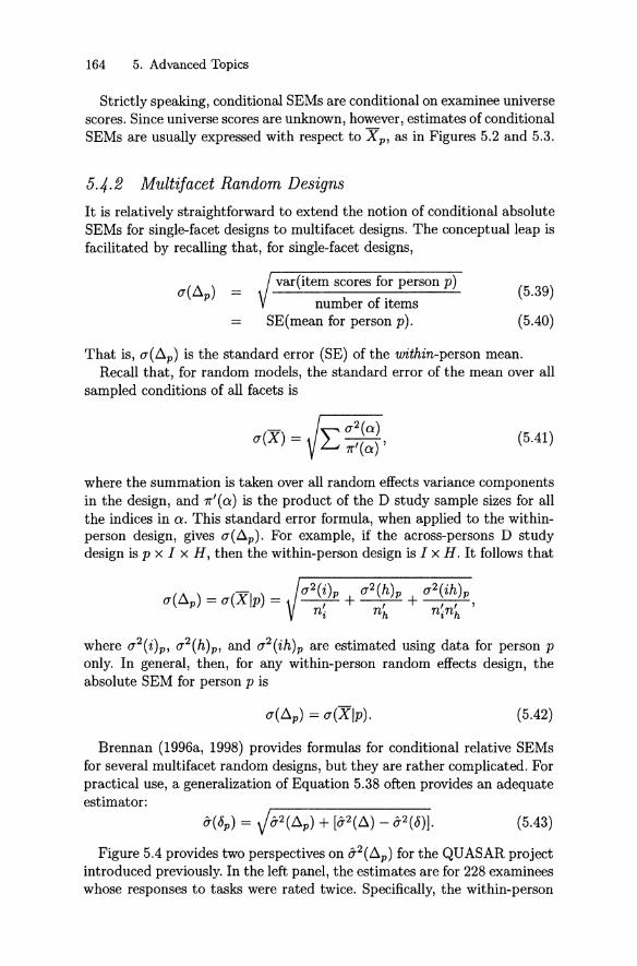
164 5. Advanced Topics

Strictly speaking, conditional SEMs are conditional on examinee universescores. Since universe scores are unknown, however, estimates of conditionalSEMs are usually expressed with respect to X p , as in Figures 5.2 and 5.3.

5.4.2 Multifacet Random Designs

It is relatively straightforward to extend the not ion of conditional absoluteSEMs for single-facet designs to multifacet designs. The conceptualleap isfacilitated by recalling that, for single-facet designs,

var(item scores for person p)

number of itemsSE(mean for person p).

(5.39)

(5.40)

That is, a(~p) is the standard error (SE) of the within-person mean.Recall that, for random models, the standard error of the mean over all

sampled conditions of all facets is

a(X) = (5.41)

where the summation is taken over all random effects variance componentsin the design, and 1T'(a) is the product of the D study sample sizes for allthe indices in a. This standard error formula, when applied to the within­person design, gives a(ßp ) . For example, if the across-persons D studydesign is p x I x H, then the within-person design is I x H . It follows that

where a2(i)p, a2(h)p, and a2(ih)p are estimated using data for person ponly. In general, then, for any within-person random effects design, theabsolute SEM for person p is

(5.42)

Brennan (1996a, 1998) provides formulas for conditional relative SEMsfor several multifacet random designs, but they are rather complicated. Forpractical use, a generalization of Equation 5.38 often provides an adequateestimator:

0-(8p) = J0-2(~p) + [o-2(~) - 0-2(8)] . (5.43)

Figure 5.4 provides two perspectives on 0-2(~p) for the QUASAR projectintroduced previously. In the left panel, the estimates are for 228 examineeswhose responses to tasks were rated twice. Specifically, the within-person

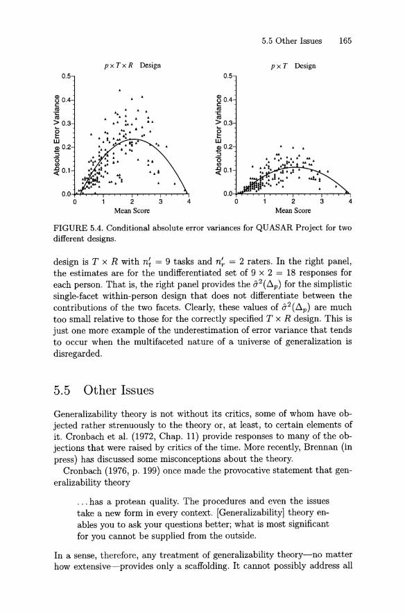
5.5 Ot her Issues 165

p xT xR Design0.5 0.5

~ 0.4 ~ 0.4c: c:l\l . . . l\l.~ '. .~.. .> 0.3 .. . .. >0.3...... .. ...e .' gw wCD 0.2 CD 0.2:; :;ö ö(J) (J)

<'i 0.1 <'i 0.1

2 3 4

Mean Score

p x T Design

. .

2 34Mean Score

FIGURE 5.4. Cond itional absolute error variances for QUASAR Project for twodifferent designs .

design is T x R with n~ = 9 tas ks and n~ = 2 raters. In the right panel ,the est imates are for the undifferentiated set of 9 x 2 = 18 responses foreaeh person. Th at is, the right panel provides the a-2 (.0.p ) for the simplisticsingle-facet within-person design that does not differentiate between thecont ributions of the two facets. Clearly, these values of a-2 (.0.p ) are muchtoo small relative to those for the correct ly specified T x R design. This isjust one more example of the underestimation of error variance that tendsto occur when the multifaeeted nature of a universe of generalizat ion isdisregarded.

5.5 Other Issues

Generalizability theory is not without its critics , some of whom have ob­jeeted rather strenuously to the theory or, at least , to cert ain elements ofit . Cronbach et al. (1972, Chap. 11) provide responses to many of the ob­jeetions that were raised by crit ics of the time . More recently, Brennan (inpress) has diseussed some misconceptions about the theory.

Cronbach (1976, p. 199) onee made the provocative statement that gen­eralizability theory

. . . has a protean quality. The procedures and even th e issuestake a new form in every context. [Generalizability] theory en­ables you to ask your questions better; what is most significantfor you cannot be supplied from the out side.

In asense, therefore, any t reatment of generalizability theory- no matterhow exte nsive--provides only a scaffolding. It cannot possibly address all

166 5. Advanced Topics

TABLE 5.7. Variance-Covariance Matrix for Person Scores for Synthetic DataSet No. 3

01

i1 i2 i3 i4

3.1667 1.0566 .8333 .88893.3889 2.2778 -.1111

2.2778 .0000.6222

Symmetrie

02

i1 i2 i3 i4

1.2778 .6667 .9444 1.5000-.1667 1.6667 .9444 .6111-.7222 1.4444 .6111 .6111.7111 -.0444 .1333 .9556

2.4556 .1556 .2556 .76671.9556 .8000 .2889

1.2111 .63332.2333

issues th at might be of concern to an investigator. In this section , a fewpotentially relevant issues are considered.

The formulas of generalizability theory are almost always presented interms of raw scores, rather than tr ansformed raw scores (i.e., scale scores).For a linear transformation E ß2 and ~ are unchanged; and 0-2(7), 0-2(0),and 0-2 (ß ) are easily obtained by multiplying the raw score values of thesestatisties by the squared slope. For nonlinear tr ansformations, however ,complexities arise, especially when replications are not available, and in­ferences must be drawn based on a single instance of the measurementprocedure. Most current research in this area has focused on condit ionalSEMs for scale scores (e.g., Kolen et al., 1992; Lee et al. , 2000) , but thereare still complexit ies and unsolved problems in applying generalizabilitytheory when average (or total) raw scores are subjected to a nonlineartransformation.

The estimat ion of variance components is clearly cent ral to applicat ionsof generalizability theory, although the theory itself is essent ially silentabout which est imation procedures are preferable. To this point , for prac­tieal and historieal reasons , the so-called ANOVA procedure for completebalanced designs has been emphasized. Using this procedure, the com­puter program GENOVA (see Appendix F) can be used for computat ions.In Chapter 7 other procedures for both balanced and unbalanced randomeffects designs are considered. The topic of estimating variance componentsis extraordinarily broad (see, e.g., Searle et al., 1992) , and sometimes usefulapproaches for specific problems are embedded in other literature (see, e.g.,Longford, 1995) .

5.5.1 Covariances as Est imators 0/ Variance Components

Relat ionships exist between random effects variance components, on theone hand, and variances and covariances of observable scores. In addit ion

5.5 Other Issues 167

to their conceptual value, these relationships can be useful for conductingsome generalizability analyses when only observed variances and covari­ances are available. Consider, for example, Table 5.7 which reports theobserved variances and covariances over persons for the Synthet ic Dat a No3 in Table 3.1 on page 72, which was used to illustrate the p x i x 0 design.Various combinat ions of the elements in thi s variance-covariance matrixcan be used to est imate certain sums of variance components.

For the p x i x 0 design,

(5.44)

where(J"2(Xpio) = E(Xpio - J-Lio)2 .

p

Note that Equation 5.44 includes all variance components that contain theindex p, the index over which variances and covariances are taken. Therelationship in Equation 5.44 also holds for estimates; that is, the averageof the variances on the diagonal of Table 5.7 equals the sum of the estimatesof the variance components , as reported in Table 3.3:

Est[E E (J"2(Xpio)]t 0

0-2(p) + 0-2(pi) + 0-2(pO) + 0-2(pio)

0.5528 + 0.5750+ 0.1009+ 0.9352

2.164,

which is identical to the average of the variances in the diagonal of Table 5.7:

(3.1667+ 3.3889 + ... + 2.2333)/8 = 2.164.

Three ty pes of covariances are identifiable in Table 5.7:

1. covariances with levels of i in common, but different levels of 0­

these are in boldface;

2. covariances with levels of 0 in common, but different levels of i­these are italicized; and

3. covariances that have neither levels of i nor levels of 0 in common­these are in normal typ e above the main diagonal.

In terms of random effects variance components for the p x i x 0 design,the expected value of the i-common covariances is:

(5.45)

where 0' is used to designate a different condit ion of the 0 facet . Thisrelationship also holds for estimates. Specifically,

Est[E E (J" (Xpio, X pio')] = 0-2(p) + 0-2 (pi) = 0.5528 +0.5750 = 1.128,t 0 ';'0'

168 5. Advanced Topics

which is identical to the average of the i-common covariances (boldfacevalues) in Table 5.7:

[1.2778 + 1.6667 + 0.6111 + 0.9556]/4 = 1.128.

Similarly, for the o-common covariances,

(5.46)

and for the covariances that have neither i nor 0 in common,

(5.47)

From Equations 5.44 to 5.47, it is evident that a variance-covariancematrix over persons for the p x i x 0 design provides sufficient informa­tion for an investigator to estimate all random effects variance componentsthat contain the person index p. It is equally evident, however, that sucha variance-covariance matrix does not provide a basis for estimating vari­ance components that do not contain p, namely, a2(i), a2(0), and a2(io).

When persons are the objects of measurement, variance components thatdo not contain p enter a2 (b.) for the p x i x 0 design. It follows that ananalysis of the properties of a measurement procedure based solelyon avariance-covariance matrix over persons is incapable of providing a basisfor estimating absolute error variance a 2(b.).

Although the above discussion has been specifically related to a variance­covariance matrix over persons for the p x i x 0 design, the basic proceduresare applicable to a variance-covariance matrix for any design. That is, thecovariances over a particular facet provide a sufficient basis for estimatingthe random effects variance components that involve that facet .

5.5.2 Estimators of Universe Scores

Observed scores are easy to compute and they are unbiased estimatorsof universe scores. Consequently, they are frequently used. However, thereare other estimators that have characteristics that are sometimes judgeddesirable.

Regressed Score Estimates

For any design, the regression equation discussed by Cronbach et al. (1972)for estimating universe scores has the general form:

(5.48)

where the parameter J..L is the grand mean for the population and universe,X p is a person's observed mean score for the particular sample of conditions

5.5 Other Issues 169

used in a D study, and the parameter p2(X p , /-L p) is t he squared correlationbetween observed and universe scores for the populat ion. T he error varianceassociated with using Pp as an estimate of /-L p is

(5.49)

where p2 is used here as an abb reviation for p2(Xp, /-Lp). Since (12(&) isgenera lly smaller than (12(ß), it is frequently stated th at it is "better" toest imate /-Lp using Pp, rath er th an X p- Such astatement , however , applies toa randomly selected person, not necessarily to a particular person. Also, fora given person, a regressed score est imate is a biased estimate of universescore. The st and ard error of est imate (1 (&) can be used to establish toleranceintervals for Pp, as discussed later in Section 12.2.4.

For th e I :p design, E pXp = /-L , and th e regression equation is

(5.50)

To use this last equation for estimat ing /-Lp we replace th e parameters p2and /-L with th e est imates E rl and X , respectively. Thi s gives

(5.51)

which is sometimes called an "est imat ion" equation to distinguish it fromth e regression Equat ion 5.50. Such point estimates of universe scores wereoriginally proposed by Kelley (1947). Equat ion 5.51 has a Bayesian in­terpretation since any such estimate is based upon information about anindividu al (his or her observed score X p) as well as information about thegroup to which the individual belongs (e.g., a sample mean X). Clearly, fora highly dependable measurement procedure, X p is weighted very heavily,and X receives relat ively little weight. By cont rast, when E {J2 is small, Ppis heavily influenced by t he group mean.

For the p x I design, E pXp = /-LI , t he regression equation is

(5.52)

and an associated est imat ion equat ion requires est imates of /-L, /-LI , and p2.Cronbach et al. (1972) suggest th at /-L can be est imated from th e G study,th e D study, or both; indeed , th ey consider myriad possibilities for esti­mating /-L. Ideally they want both /-LI and p2 to be est imated for the fixedset of items in a par ticular D study. In practice, however, their est ima­t ion equations usually necessit ate one or more of the classical test theoryassumptions of equal means, equal variances, and equal correlations of ob­served and universe scores. When all of these assumpt ions are made, th eest imation equation for the p x I design is identical to Equation 5.51 forthe I:p design. When the classical assumpt ions are relaxed, t he result ingest imation equations are probably best viewed as ad hoc approximations

170 5. Advanced Topics

with properties that are difficult to ascertain (see Cronbach et al., 1972,pp . 138ff).

Although we have focused here on single-facet designs, Equations 5.48and 5.49 apply to any design. In practice, estimates are required for E p2

and JL , as well as JLn if the design is not fully nested.!?

Best Linear Prediction

Jarjoura (1983) suggested that theoretical developments in the area of"best" linear prediction functions (see Searle, 1974; Searle et al., 1992) canbe used to derive predictors of universe scores that have certain optimalproperties. These prediction functions have some similarities with regressedscore estimates, but neither the derivation nor the est imation of such pre­diction functions necessitates any of the classical test theory assumptionsor any assumptions about distributional form. For a p x I design, assum­ing G and D study sample sizes are the same, the best linear predictionfunction for universe scores is

fi,p = JL + A(X - JL) + B(Xp - X), (5.53)

where X p is a person's observed mean score for a particular sample of items(i.e., a particular test form), X is the mean of X p over a sample of persons,

andB = a

2 (p)a2(p) + a2(pi)jn i

The error variance associated with using fi,p as an estimate of JLp is

(5.54)

The last term in the prediction function in Equation 5.53 adjusts X p forthe relative difficulty of a particular test form, and th e second term can beviewed as a correction to this adjustment. Note that B has the form of ageneralizability coefficient. For the nested design, the prediction functionand regression equation are identical , even though the assumpt ions under­lying the two approaches are different. However, for the crossed design, theregression equation has no term corresponding to the second term in theprediction function . Furthermore, for the crossed design, Cronbach et al.(1972) want p2 in the regression equation to be dependent upon the par­ticular form of a test used in a D study. By cont rast , the pararnetcrs A andB in the best linear prediction function are für all randomly parallel formsof a test with a constant number of items.

10/Ln is th e rnean für the randorn facets .

5.5 Other Issues 171

In practice, to use the prediction function in Equation 5.53, an inves­tigator must estimate fl and the variance components (72(p) , (72(i), and(72 (pi) . It is highly desirable that est imates of these parameters be based onmultiple test forms , perhaps by averaging the sampIe means and estimatedvariance components for each of the forms. This approach to estimating theparameters of the prediction function is conceptually simple, but it doesrequ ire the actual existence of multiple test forms, not just an assumptionabout the possibility of multiple forms. There are other approaches to esti­mation, but any reasonably defensible approach would seem to necessitatea larger sampIe of items than those in a particular form of a test.

Subgroup Regressions

Nothing in the theory of regressed score estimates (or best linear predic­tors) requires categorizing a population of persons into different predefinedsubgroups and regressing the observed score for a person to the mean ofthe subgroup into which the person is categorized. However, this practiceis common enough to merit some consideration here. Such practice forcesan investigator to specify a variable (e.g., gender, race, or ethnicity) to beused as a basis for defining group membership , and the choice of a groupingvariable can substantially influence the mean to which an individual exami­nee's observed score is regressed. Consequently, an individual exa minee canhave as many possibly different estimates of fl p as t here are subgroups intowhich such an examinee might be classified.

Furthermore, th e use of regressed score est imates with subgroups canhave unintended negative consequences. For example , suppose that mem­bers of a minority group score lower , on the average, than members of amajority group on some test. Also, suppose that p2 is the same for bothgroups, and separate regression equat ions are used that regress minoritygroup memb ers to their mean and majority group members to their mean .Now, consider a minority and majority examinee who get the same ob­served score, which is between the mean for the minority and the majoritygroups. In this case, th e majority examinee's observed score will be re­gressed upward , the minority examinee's observed score will be regresseddownward, and th e difference between their est imated universe scores couldbe substantial if the group means were quite different .

These comments do not necessarily mean that regressed score estimatesare to be avoided when subgroups are involved. However, investigators areadvised to give careful considerat ion to the consequences of using regressedscore est imates (or best linear predictors) with subgroups.

5.5.3 Random Sampl ing Assumptions

Any theory necessarily involves cert ain assumptions t hat are idealized tosome exte nt, and in inferenti al stat ist ical theories, assumptions are always

172 5. Advanced Topics

made about random sampling, independence, and/or uncorrelated effects.Some investigators find random sampling assumptions less appealing, butrandom sampling explanations are often used to justify assumpt ions ofindependence or uncorrelated effects.

Also, generalizability theory does not dictate that, say, all of the items ina test must be considered to be a random sample from the same undiffer­entiated universe of items. This point was illustrated in examples of tablesof specifications. Almost always, one can structure a universe in such away that random sampling assumptions become more acceptable. Doing somay render a universe more complex, but serious consideration of universesfrequently reveals that they are indeed complex, without even consideringsampling assumptions.

Furthermore, random sampling assumpt ions are not unique to general­izability theory. For example, in introducing their treatment of item sam­pling, Lord and Novick (1968, p. 235) offer the followingrationale in supportof random sampling assumpt ions in test theory.

A possible objection to the item-sampling model (for exam­ple, see Loevinger, 1965) is that one does not ordinarily buildtests by drawing items at random from a pool. There is, how­ever, a similar and equally strong objection to classical test the­ory: Classical theory requires test forms that are strictly paral­lel, and yet no one has ever produced two strictly parallel formsfor any ordinary paper-and-pencil test. Classical test theory isto be considered a useful idealization of situations encounteredwith actual mental tests. The assumption of random samplingof items may be considered in the same way. Further, even ifthe items of a particular test have not actually been drawn atrandom, we can still make certain interesting projections: Wecan conceive an item population from which the items of thetest might have been randomly drawn and then consider thescore the examinee would be expected to achieve over this pop­ulation. The abundant information available on such expectedscores enhances their natural interest to the examiner.

In a related vein, but in the broader context of inferential statistics,Cornfield and Tukey (1956, pp. 912-913) discuss a "bridge analogy" thathas become a famous defense of random sampling assumptions.

In almost any practical situation where analytical statisticsis applied, the inference from the observations to the real con­clusion has two parts, only the first of which is statistical. Agenetic experiment on Drosophila will usually involve flies ofa certain race of a certain species. The statistically based con­clusions cannot extend beyond this race, yet the geneticist willusually, and often wisely, extend the conclusion to (a) the whole

5.5 Other Issues 173

species, (b) all Drosophila, or (c) a larger group of insects . Thiswider extension may be implicit or explicit , but it is almost al­ways present . If we take the simile of the bridge crossing a riverby way of an island , there is a statistical span from t he nearbank to the island , and a subject-matte r span from the islandto th e far bank . Both are important .

By modifying the observation program and the correspond­ing analysis of the dat a, the island may be moved nearer to orfarther from the dist ant bank , and the stat ist ical span may bemade st ronger or weaker . In doing th is it is easy to forget thesecond span, which usually can only be strengthened by im­proving the science or art on which it depends . Yet a balancedunderst anding of, and choice among, the statistical possibilitiesrequires constant at tent ion to the second span. It may often beworth while to move the island nearer to the distant bank , atthe cost of weakening the stati stical span-particularly whenthe subject-matter span is weak.

In an experiment where a population of C columns was spec­ified, and a sampie of c columns was randomly selected, it isclearly possible to make analyses where

1) the c columns are regarded as a sampie of c out of C, or2) the c columns are regarded as fixed.

The questions about these analyses is not their validity but th eirwisdom.... The analyses will differ in the length of their infer­ences; both will be equally st rong statistically. Usually it willbe best to make analysis (1) where the inference is more gen­eral. Only if this analysis is entirely unrevealing on one or morepoints of interest are we likely to be wise in making analysis(2), whose limited inferences may be somewhat revealing.

But what if it is unreasonable to regard c columns as anysort of a fair sampie from a population of C columns with C > c.We can (at least formally and numerically) carry out an anal­ysis with , say, C = 00 . What is the logical position of suchan analysis? It would seem to be much as folIows: We cannotpoint to a specific population from which the c columns were arandom sampie, yet the final conclusion is certainly not to justthese c columns. We are likely to be better off to move the is­land to th e far side by introducing an unspecified population ofcolumns "like th ose observed" and making the inference to themean of this population. This wililengthen the st atistical spanat the price of leaving the location of the far end vague. Unlessthere is a known fixed number of reasonably possible columns,this lengthening and blur ring is likely to be worthwhile.

174 5. Advanced Topics

In short, there is considerable precedent for random sampling assump­tions in many statistieal and psychometrie theories. To say that such as­sumptions are idealized to some extent is hardly a compelling reason toreject them categorieally, partieularly in generalizability theory where thecentral focus is on generalization from a sample of conditions of measure­ment to a universe of conditions of measurement.

5.5.4 Generalizability and Other Theories

At various points in this book, relationships between generalizability theoryand classieal test theory have been discussed. Provided below are brief con­siderations of some similarities and dissimilarities between generalizabilitytheory and three other psychometrie theories.

Covariance Structure Analysis

The discussion of variance-covariance matrices in Section 5.5.1 has ties tocovariance structure analysis and structural equation modeling (see, e.g.,Jöreskog & Sörbom, 1979, and Bollen, 1989), although these methodolo­gies have a much broader scope of inquiry than merely estimating randomeffects variance components (Linn & Werts, 1979) using computer pro­grams such as LISREL (Jöreskog & Sörbom, 1993). Many applications ofthese methodologies are more directly related to multivariate generalizabil­ity theory (see Chapters 9 to 12), which involves specific variance and co­variance components for different fixed strata. Even in such cases, however,the assumptions in covariance structure analysis and structural equationmodeling are usually stronger than those in generalizability analyses . Also,covariance structure analyses and structural equation modeling do not em­phasize generalizations from a sample of conditions of measurement to anexplicitly defined multifaceted universe of conditions of measurement, atleast not to the same extent that generalizability theory does. Even withthese discontinuities, however, covariance structure analyses and structuralequation modeling have potential applicability in generalizability theory.

In asense, covariance structure analysis and structural equation model­ing are extensions of procedures for examining the effects of measurementerror on independent variables in regression analyses. The basie idea behindsuch analyses is summarized by Snedecor and Cochran (1980, pp. 171-172) ,and Fuller (1987) devotes much of his book on Measurement Error Mod­els to this topie . The title of Fuller's book suggests a strong relationshipbetween these models and generalizability theory. There are important dif­ferences, however. Foremost among them is that generalizability theoryrequires that the investigator carefully define the types of errors of inter­est, and generalizability theory focuses on quantifying and understandingthe various sources of measurement error for all variables of interest. Still,

5.5 Other Issues 175

there are similarit ies between some aspects of genera lizability theory andregression analyses with fallible independent variables.

Multiple Matrix Sampling

T here are some similarities between generalizability theory and multipl ematrix sampling theory (see Lord & Novick, 1968, Chap. 11; and Sirot­nik & Wellington, 1977). Both are sampling theories and both considerthe est imation of variance components and their standard errors. Gener­alizability theory, however , involves a concept ual framework that is con­siderably broader than multiple matrix sampling. Also, the two theoriesemphasize different issues and frequently define and est imate parametersin a somewhat different manner. The simplest multiple matrix samplingdesign involves randomly partitioning th e finite universe of items to k sub­universes, randomly partitioning the finite population of persons into ksubpopulat ions, and then randomly pairing the subuniverses and subpopu­lations. These subuniverses and subpopulations are not fixed st rata in thesense discussed in generalizability theory, however.

Also, for sampling from a finite population and /o r universe, variancecomponents are sometimes defined differently in mult iple matrix samplingand genera lizability theory. For example, Sirotnik and Wellington's (1977,p. 354) variance components (called (j2-terms) are not identieal to thosebased on t he Cornfield and Tukey (1956) definitions, whieh are the defini­t ions usually employed in genera lizability theory.

In mult iple mat rix sampling, using generalized symmetrie sums or means,variance components can be estimated for complicated designs with or with­out missing data, and higher-order moments of distribut ions can be esti­mated. Doing so is computationally intensive, but these procedures meritfurther consideration in the context of genera lizability ana lyses.

Item Response Theory

Some believe that item response theory will replace most other measure­ment theories in the future. This author is unconvinced, however. It seemsunarguable th at , if certain (rather strong) assumptions are fulfilled, thenitem response th eory provides a powerful model for addressing a number ofimportant psychometrie issues th at are not easily t reated with ot her theo­ries, including generalizability theory. However , even if these assumpt ionsare fulfilled, item response theory does not easily accommodate generaliza­t ions to multifaceted universes.

Item response theory pays attention to individual items as fixed entitieswithout specific consideratio n of other conditions of measurement . By con­t rast , in generalizability theory, items are generally viewed as random andemphasis is placed on viewing them as sampled conditions of measurement.There are, of course, ot her differences between the two theories, but thefixed/random difference is fundamental. A few efforts have been made to

176 5. Advanced Topics

link the theories (e.g., Kolen & Harris, 1987; Bock et al., 2000) but in t hisauthor's opinion, one theory is not properly viewed as a replacement forthe other. Generalizability theory is primarily a sampling model, whereasitem response theory is principally a scaling model.

5.6 Exercises

5.1* For the APL Survey D st udy design in Table 5.1, each person re­sponds to the same set of items. Suppose, however , that each persontook a different set of eight items for each content area. What isthe notational repr esentation of this design? Wh at are the est imatedG study and D study variance components? What are 0-2(7), 0-2(6),0-2(~) , E{J2, and ~?

5.2* Using the APL Survey Instrument discussed in Sections 3.5 and 5.1.3a test-retest st udy was conducted in which 206 examinees took thesame form of the Survey on two occasions. The resultin g mean squareswere as folIows.

Effect MB Effect MB Effect MB

p 2.9304 po .2085 oi :h .17420 .6068 ph .2767 poh .1089h 18.4148 pi:h .2406 poi:h .0825i :h 10.6986 oh .5290

Provide the notational representation, Venn diagram, and linearmodel for this G study design. What are the estimated G st udy vari­ance components for the model in which content areas are fixed? Ifgeneralizat ion is intended for a single randomly selected occasion andn~ = 8, what are the D st udy variance components, 0-2(7), 0-2(6), andE {J2?

5.3* Why is the value of E {J2 from Exercise 5.2 considerably smaller thanthe value of E{J2 = .905 in Table 5.1? If the result s in Table 5.1were unknown , but the results from Exercise 5.2 were available, whatwould be reasonable est imates of (12 (7), (12 (6), and E p2 under theassumptions implicit in Table 5.1?

5.4 Verify th at Equation Sets 5.16 and 5.17 apply to the est imates re­ported in Tables 5.5 and 5.6 for the APL Survey.

5.5 Given the Cornfield and Tukey definitions of variance components inTable 5.6 and the definition of (12(7) in Equation 5.18, prove that

n -1(12(7) = _r_(12(r IRH) + (12(p:r IRH).

n r

5.6 Exercises 177

Hint : The proof involves careful consideration of model restrictions,as discussed in Section 3.5.

5.6 Using only the variance components in Table 5.6, what is an est imateof E p2 for a randomly selected region?

5.7* Shavelson et al. (1993) provide an example of a voluntary statewidescience assessment program in which st udents (p) in approximately600 schools (g) took five performance tasks (t) . For a subset of theirresults:

For thes e data:

(a) show that Inequality 5.25 is not satisfied; and

(b) provide a few values of np and ni th at lead to a contradiction ofthe conventional wisdom that Ep; > Ep~ .

5.8 When both persons and items are random, prove that a2(8g ) > a2 (8p )

implies th at Inequality 5.28 is satisfied.

5.9* Consider , again, Exercise 2.1. For each of th e six persons determineO'(~p) for n~ = 3 and verify that the average of the squares of theseestim ated conditional SEMs is 0'2(~) .

5.10 For the ITED Vocabulary example in Section 5.4.1, O'2(~) = .00514and 0'2(8) = .00475. For examinees with X p = .6, show that thequadrati c fit and Equation 5.38 give very similar values for O'(8p).

5.11 In Section 5.5.1, the expressions for covariances in terms ofrandom ef­feets variance components are expressed for single conditions of facets(lowercase letters) . Th ese relationships also hold for means over setsof conditions for facets. For Synthetic Data No. 3 in Table 3.1 onpage 72, verify th at

6Variability of Statistics inGeneralizability Theory

Estimates of variance components, error variances , generalizability coef­ficients, and so on, like all statistics, are subject to sampling variability.Traditionally, such variability is quantified through estimated standard er­rors and/or confidence intervals . Cronbach et al. (1972) recognized theimportance of this topic for generalizability analyses and gave it more thanpassing attention, although at that time statistical methodologies for ad­dressing the topic were limited. Subsequently, in the generalizability the­ory literature, Smith (1978, 1982) considered standard errors of estimatedvariance components, Brennan (1992a) summarized some procedures for es­tablishing standard errors and confidence intervals, Brennan et al. (1987)considered bootstrap and jackknife procedures, Betebenner (1998) exam­ined a relatively new procedure for establishing confidence intervals , Wiley(2000) studied the bootstrap, and Gao and Brennan (2001) provided ex­amples from the performance assessment literature.

In the statistical literature, assuming score effects are normally dis­tributed, Searle et al. (1992) treat in detail standard errors for estimatedvariance components,' and Burdick and Graybill (1992) provide a verycomprehensive and readable treatment of confidence intervals for variancecomponents and various ratios of them.

This chapter summarizes most methodologies that have been developedto estimate standard errors and confidence intervals for (estimated) vari-

1 In many resp ects, Searle et a l. (1992) build on the seminal work reported two decadesearlier by Searle (1971) .

180 6. Variability

ance components. These are complicated matters with many unsolved prob­lems, especially when score effects are not normally distributed. Most ofthe procedures discussed apply, at least in theory, to random effects vari­ance components for any balanced design. However, examples, simulations,and exercises are largely specific to the p x i and p x I designs. Extensionsto other designs are evident for some procedures, but largely unstudied forothers. The goal of this chapter is simply to introduce students and prac­titioners of generalizability theory to the methodologies, as they apply ingeneralizability theory. Much research remains to be done.

Most notational conventions in this chapter are the same as those used inprevious chapters. The most noteworthy exception is that a variation on thenotation in Burdick and Graybill (1992) is employed for some procedures.This leads to some notational inconsistencies between parts of this chapterand the rest of this book. Such inconsistencies are identified when theyarise.2

6.1 Standard Errors of Estimated VarianceComponents

In principal, standard errors of estimated variance components can be esti­mated by replicating a study and computing the standard deviation of theresulting sets of estimates. In theory, this procedure has much to recom­mend it (see Brennan, in press). It is directly related to the basic notionof generalizing over randomly parallel instances of a measurement pro­cedure, it is computationally straightforward, and it is empirically basedwithout distributional-form assumptions. For example, Table 6.1 providesestimated variance components for nine forms on one mathematics sub­test of the ACT Assessment (ACT, 1997). The data were collected for anequating study in which all forms were administered to randomly equiva­lent groups . Consequently, the standard deviations in the next-to-the-lastrow are direct empirical estimates of the standard errors of the estimatedvariance components.

Estimated standard errors such as those in Table 6.1 are elose to idealin the sense that they require minimal assumptions. In many contexts,however, replications are simply not available, In the absence of replica­tions, there are two general elasses of procedures for estimating standarderrors. One elass makes assumptions about the distributional form of theeffects, usually multivariate normality. The other dass involves resamplingmethods such as the jackknife and bootstrap.

2It is possible to resolve these notational inconsistencies, but doing so would cornpli ­cate matters substantially for readers who study the literature cited in this chapter.

6.1 Standard Errors of Estimated Variance Components 181

TABLE 6.1. c Study p x i Results for Nine Forms of ACT MathPre-AlgebrajElementary Algebra Subtest with 24 Items

Form np MS(p) MS(i) MS(pi) a-2 (p) a-2 (i) a-2(pi)

A 3388 .9472 85.9556 .1768 .0321 .0253 .1768B 3363 1.0621 91.5600 .1517 .0379 .0272 .1517C 3458 .8872 127.2861 .1421 .0310 .0368 .1421D 3114 .9031 96.5736 .1671 .0307 .0310 .1671E 3428 1.1280 63.5186 .1712 .0399 .0185 .1712F 3318 .9601 136.5013 .1599 .0333 .0411 .1599G 3257 .8828 95.1346 .1717 .0296 .0292 .1717H 3221 .8448 161.2862 .1579 .0286 .0500 .1579I 3178 .8646 94.8867 .1724 .0288 .0298 .1724

Mean .0324 .0321 .1634SD .0040 .0093 .0114Ave SEa .0010 .0094 .0008

aSquare root of the average of the squared estirnated standard errors using Equa-tion 6.!.

6.1. 1 Normal Procedure

The traditional approach to est imat ing standard errors of esti mated vari­ance components assurnes that score effect s have a multivariate normaldistribution . Under this assumption, it can be shown (see Searle 1971, pp .415-417; Searle et al. 1992, pp . 137-138) that an est imator of the standarderror of an estimated variance component is

"" 2[J(ßla )MS( ß)j27 df (ß) + 2 '

(6. 1)

where M design ates t he model, ß ind exes the mean squares that entera-2 (a IM ), and f (ßla ) is t he coefficient of MS (ß) in t he linear combinati onof mean squares that gives a-2 (a jM ). The squar e of t he right-hand side ofEquation 6.1 is an unbiased est imator of the vari an ce of a- 2 (a IM ). For aran dom effects model, a slightly simpler version of Equation 6.1 is

L 2[MS(ß)]2ß df( ß) + 2 '

(6.2)

where, as in previous chapters, 7l" (ä) is the product of the sample sizes forindices not in a .3

3Equation 6.1 applies to both G study and D study variance cornponents (includingerror variances) that can be expressed as linear cornbinations of rnean squares. Equa­tion 6.2 , however, should be used only for G study randorneffects variance cornponents.

182 6. Variability

TABLE 6.2. G Study Results for Synthetic Data Set No. 4 Recast as a p x iDesign

Estimated Standard Errors

df MB Normal Jackknife Ratio"

p 9 10.2963 .6258 .3673 .4254 1.542011 11.6273 .8840 .4577 .5551 1.7774

pi 99 2.7872 2.7872 .3922 .5569 7.0356aRatio of est imated variance component to est imated st andard error, with th e latter

computed using df rather th an df + 2 in Equ ation 6.1.

It is evident from the form of Equation 6.1 that estimate d standarderrors decrease as degrees of freedom (i.e., sarnple sizes) increase. Also,ot her things being equal, est imated standard errors are likely to be smallerfor est imated variance components that involve fewer mean squares. Forthis reason , all other things being equal, the estimated vari ance componentfor a nested effect involving k indices (e.g., i:h) will have a smaller st anda rderro r than for an int eraction effect involving the same kindices (e.g., ih).

Consider again the Synthetic Dat a Set No. 4 in Table 3.2 on page 73recasting it as a p x i design with n p = 10 persons and ni = 12 items.Table 6.2 provides the typical ANOVA results, the est imated variance com­ponents, and the estimates of t he standard errors of the est imated variancecomponents using Equation 6.2. As might be expected with such smallsample sizes, t he estimated standa rd errors are substantial. Of course, wedo not know whether the normality assumptions are sensible for t hese dat a.

Wh en normality assumptions are violat ed , Equ ations 6.1 and 6.2 maygive misleading results. Consider , again, the result s in Table 6.1 for nineforms of an ACT Assessment Mathematics subtest . Each form is basedon 24 dichotomously scored items. The last row in Table 6.1 reports theaverages of the standard errors est imated using Equation 6.2, althoughthere is good reason to believe that normality assumptions are not fulfilledfor these data. Clearly, for a2 (p) and particularly a2(pi ), the normality­based average estimates in the last row are substantially smaller than thepreferable est imates in the next-to-the-last row.

6.1.2 Jackknife Procedure

Quenouille (1949) suggeste d a nonparametric est imato r of bias, Tukey(1958) extended Quenouille's idea to a nonp arametric estimator ofthe stan­dard erro r of a statistic. The theory underlying the jackknife is discussedexte nsively by Shao and Tu (1995). Here, we briefly outline the basics ofthet heory and t hen discuss its application to est imate d variance componentsfor t he p x i design.

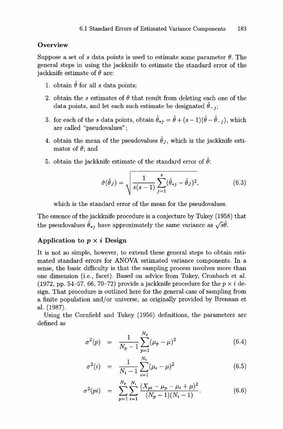
6.1 Standard Errors of Estimated Variance Components 183

Overview

Suppose a set of 8 data points is used to estimate some parameter B. Thegeneral steps in using the jackknife to estimate the standard error of thejackknife estimate of Bare:

1. obtain 8for all 8 data points;

2. obtain the 8 estimates of B that result from deleting each one of thedata points, and let each such estimate be designated 8_j;

3. for each of the s data points, obtain 8*j = 8+ (8-1)(8- 8_ j), whichare called "pseudovalues" ;

4. obtain the mean of the pseudovalues 8J, which is the jackknife esti­mator of B; and

5. obtain the jackknife estimate of the standard error of 8:

(6.3)

which is the standard error of the mean for the pseudovalues.

The essence of the jackknife procedure is a conjecture by Tukey (1958) thatthe pseudovalues 8*j have approximately the same variance as .;s8.

Application to p X i Design

It is not so simple, however, to extend these general steps to obtain esti­mated standard errors for ANOVA estimated variance components. In asense, the basic difficulty is that the sampling process involves more thanone dimension (i.e., facet) . Based on advice from Tukey, Cronbach et al.(1972, pp . 54-57, 66, 70-72) provide ajackknife procedure for the p x i de­sign. That procedure is outlined here for the general case of sampling froma finite population and/or universe, as originally provided by Brennan etal. (1987).

Using the Comfield and Tukey (1956) definitions, the parameters aredefined as

(6.4)

(6.5)

(6.6)

184 6. Variability

Letting cp = 1 - np/Np and Ci = 1 - ni/Ni be finite population/universecorrection factors, the estimators of the variance components are:

a-2 (p)

a-2 (i)

a-2 (pi)

[MS(p) - Ci MS (pi)J!ni

[MS(i) - epMS(pi)J!np

= MS(pi ).

(6.7)

(6.8)

(6.9)

Obviously, these equations give the usual random effects est imates whenCp =Ci = 1.

Consider the following notational convent ions.

B= any estimated variance component for t he p x i design based onanalyzing t he full np x ni matrix [i.e., B could be a-2 (p), a-2 (i) , ora- 2 (pi)];

B_pi = value of B for the (np -1) x (ni - 1) matrix that results fromdelet ing person p and item i;

B-pO = value of Bfor the (np- 1) x ni matrix that results from deletingperson p;

B-Oi = value of Bfor the np x (n, - 1) matrix that results from deletingitem i; and

B-oo = value of B for t he original np x ni matrix (i.e., B= B-oo).

Given these not ational conventions, the pseudovalue for person p and itemi is

B*Pi = npniB-oo - (np - l)niB_po - np(ni - l )B- oi + (np - l)(ni - l)B_pi,(6.10)

and the mea n of t he pseudovalues is the jackknife estimator of ():

(6.11)

For the ANOVA estimators of variance components, BJ = B.The standard error of BJ = Bis estimated using the matrix of pseudoval ­

ues, which has np rows and ni columns. Note that there is one such matrixfor each of the three estimated variance components. For any one of theseestimated variance components, let a-2 (rows) , a-2 (cols), and a- 2 (res) be theestimated variance components for the matrix of pseudovalues. Then, the

6.1 Standard Errors of Estimated Variance Components 185

estimate d st andard error of 0J is4

(6.12)

Table 6.2 provides the jackknife est imates of the three variance compo­nents for t he synthetic data example. The principal advantage of these es­timates is t hat they are not based on any distributional-form assumptions.The principal disadvantage is that exte nsive computat ions are required.Even for t his very small set of synt hetic dat a , each of t he three jackknifeest imates requires computing 11 x 13 = 143 sets of est imated variance com­ponents that are t he basis for the final computations using Equ ation 6.3.

6.1. 3 Bootstrap Procedure

The bootstrap is similar to the jackknife in that both are resampling pro­cedures and both are prim arily nonparametric methods for assessing theaccuracy of a par ticular 0as an est imate of B. A prin cipal difference betweenthe two procedures is that t he bootstrap employs sampling with replace­ment, whereas t he jackknife employs sampling wit hout replacement. Efron(1982) provides an early t heoretical t reatment of t he boot strap ; Efron andTibshirani (1986) provide a simpler and more applied t reatment; and Shaoand Tu (1995) provid e a recent extensive treatment.

Overview

For a stat ist ic based on s observations, the bootstrap algorithm is basedon multiple bootstrap samples, with each such sample consist ing of a ran­dom sample of size s witk replacement from t he original sample. Using t heboot strap , est imation of t he st andard error of a stat ist ic 0 involves thesesteps:

1. using a ra ndom number generator, independent ly dr aw a large num­ber of bootstrap samples, say B of them;

2. for each sample, evaluate the statist ic of inte rest, say Ob (b = 1, ... , B );and

3. calculate the sampie st anda rd deviat ion of t he Ob:

(6.13)

4In their discussion of thejackknife, Cronbach et al. (1972, pp. 56 and 71) incorrectIysuggest that this result be divided by Jnp n; . Also, they suggest jackknifing the loga­rithms of the estimated variance components rather than the cstimates themselves; thisauthor's research does not support doing so.

186 6. Variability

where

(6.14)

is the bootstrap estimate of e.

Note that the bootstrap standard error in Equation 6.13 has the form ofa standard deviation, whereas the formula for the jackknife standard errorin Equation 6.3 has the form of a standard error of a mean .

Application to p X i Design

Although the bootstrap is conceptually simple, it is not unambiguouslyclear how to extend it to the random effects p x i design, which involvestwo dimensions/facets. Difficulties were originally discussed by Brennanet al. (1987) and subsequently by Wiley (2000) .5 The crux of the matteris specifying how to draw bootstrap sampies from the np x ni matrix ofobserved scores. It might seem that the obvious approach is to:

1. draw a sampie of n p persons with replacement from the sampledpersons;

2. draw an independent random sampie of ni items with replacementfrom the sampled items; and

3. let the bootstrap sampie consist of the responses of the sampled per­sons to the sampled items.

This double sampling procedure is designated "boot-p, i."It is important to note that the boot-p, i procedure involves sampling

with replacement, which means that any bootstrap sampie likely will con­tain some repeated persons and some repeated items. This characteristic ofthe boot-p , i procedure introduces bias in estimates of some variance com­ponents (i.e., OB in Equation 6.14 is sometimes biased), which certainlycasts doubt on the accuracy of any associated confidence intervals. For ex­ample, in a random effects design, the ANOVA estimate of &2(p) is usuallyexpressed as [MS(p) - MS(pi)]/ni' but an equivalent expression is

(6.15)

which is the average of the estimates of the item covariances. When itemsare repeated, Equation 6.15 suggests that &2(p) is likely to be an inflatedestimate of a2 (p), especially when ni is relatively smalI. A similar statementholds for &2 (i).

5See also Leucht and Smith (1989) and Othman (1995) .

6.1 Standa rd Errors of Estimated Variance Components 187

Brenn an et al. (1987) suggested three other procedures for obtainingbootstrap samples." The boot-p procedure involves sampling np personswith replacement, but not items. The boot- i procedure involves samplingn i items with replacement , but not persons . The boot-p and boot-i pro­cedures keep items and persons fixed, respectively, in obtaining bootstrapsampies. Since results are desired for a design in which both persons anditems are random, it is to be expected that neither of th ese procedures willbe completely sat isfactory for est imat ing standa rd errors for all esti matedvariance components.

The final procedure suggested by Brennan et al. (1987) is the boot-p , i, T

procedure in which persons, items, and residuals are each sampled withreplacement . RecaB from Section 3.3.2 that , in terms of observed-scoreeffects ,

X pi X + x p + Xi + Tpi

X + (X p - X ) + (X i - X) + (Xpi - X p - X i + X) ,

where, for our purposes here, Tpi is used to designate the residual effect. Theboot-p , i, T procedure involves using a random sampie with replacement ofsize np from the set of x p , an independent random sampie with replacementof size ni from the set of Xi, and an independent random sampie withreplacement of size npni from th e set of Tpi' It is import ant to note thatth e sampling of th e three effects is independent . So, for example, if the firstperson sampled for x p were 12, and the first item sampled for Xi were 15,only by chance would th e sampled residual be th e residual associated withperson 12 and item 15 in the original data.

Intuition and logic such as th at discussed in conjunct ion with Equa­tion 6.15 suggest that none of th ese bootstrap procedures is likely to leadto unbiased est imates of variance components . Wiley (2000) formalizedt hese intuit ive not ions and derived the result s in Figure 6.1 th at adjust forbias induced by the various bootstrap sampling procedures. For example,if boot-p is used to estimate a2(p) or th e stand ard error of 0-2(p), then thebootstrap est imates should be multiplied by np/(np - 1).

For the synt het ic dat a example introduced in Section 6.1.1, Table 6.3provides both unadjusted and adjusted bootstrap means and est imatedstandard errors for 0-2(p), 0-2(i), and 0-2(pi) based on th e four bootstrapsampling procedures introduced above. The result s in Table 6.3 are basedon 1000 replications. For example, the adjusted boot-p value of .6185 forthe mean of 0-2(p) was obtained as folIows.

1. Obtain a bootst rap sampie using the boot-p procedure,

2. for this bootstrap sampie, compute the usual ANOVA esti mate ofa2(p) and designate it 0-2(plboot-p),

6W iley (2000) has sugges ted a few other bootstrap procedu res not considered here.

188 6. Variability

Adjusted Estimates Based on boot-p

= ~ &2(plboot-p)np - 1

&2(i lboot-p) _ _ 1_ &2(pi Iboot-p)np -1

= ~ &2(pil boot-p)n p - 1

Adjusted Estimates Based on boot-i

n i A2("b ')-- er t oot-zni - 1

&2(plboot-i) __1_ &2(pi lboot-i)n i - 1

~ &2(pi lboot-i)ni - 1

Adjusted Estimates Based on boot-p, i

Adjusted Estimates Based on boot-p, i , r

FI GURE 6.1. Wiley's adjustments for bias in bootstrap procedures for estimatingvariance components and their standard errors .

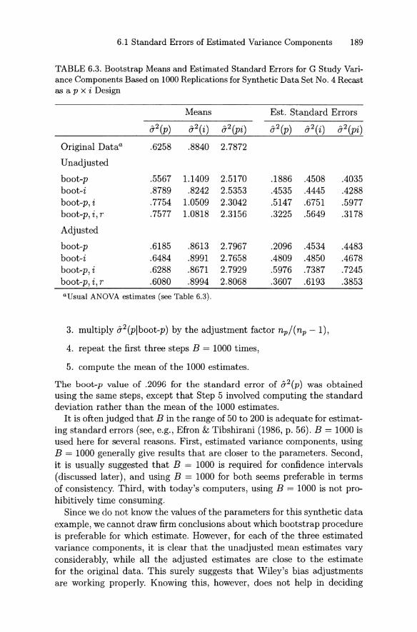
6.1 Standard Errors of Estimated Varianee Components 189

TABLE 6.3. Bootstrap Means and Estimated Standard Errors for G Study Vari­anee Components Basedon 1000 Replieations forSynthetie Data Set No. 4 Reeastas a p x i Design

Means Est. Standard Errors

0-2(p) 0-2(i) 0-2(pi) 0-2(p) 0-2(i) 0-2(pi)

Original Dataa .6258 .8840 2.7872

Unadjusted

boot-p .5567 1.1409 2.5170 .1886 .4508 .4035boot-i .8789 .8242 2.5353 .4535 .4445 .4288boot-p, i .7754 1.0509 2.3042 .5147 .6751 .5977boot-p, i , r .7577 1.0818 2.3156 .3225 .5649 .3178

Adjusted

boot-p .6185 .8613 2.7967 .2096 .4534 .4483boot-i .6484 .8991 2.7658 .4809 .4850 .4678boot-p, i .6288 .8671 2.7929 .5976 .7387 .7245boot-p, i, r .6080 .8994 2.8068 .3607 .6193 .3853

aUsual ANOVA estimates (see Table 6.3).

3. multiply 0-2(plboot-p) by the adjustment factor npj(np - 1),

4. repeat the first three steps B = 1000 times,

5. compute the mean of the 1000 estimates.

The boot-p value of .2096 for th e standard error of a-2 (p ) was obtainedusing the same steps, except that Step 5 involved computing the standarddeviation rather than the mean of the 1000 estimat es.

It is often judged that B in the range of 50 to 200 is adequate for estirnat­ing standard errors (see, e.g., Efron & Tibshirani (1986, p. 56). B = 1000 isused here for several reasons. First, estimated variance components, usingB = 1000 generally give results that are eloser to the parameters. Second,it is usually suggested that B = 1000 is required for confidence intervals(discussed later) , and using B = 1000 for both seems preferable in termsof consistency. Third, with today's computers, using B = 1000 is not pro­hibitively time consuming.

Since we do not know the values of the parameters for this synthetic dataexample, we cannot draw firm conelusions about which bootstrap procedureis preferable for which est imate. However, for each of the three estimatedvariance components, it is elear that the unadjusted mean estimates varyconsiderably, while all the adjusted estimates are elose to the estimatefor the original data. This surely suggests that Wiley 's bias adjustmentsare working prop erly. Knowing this, however, does not help in deciding

190 6. Variability

which bootstrap procedure is preferable for estimating standard errors.Some guidance is provided by simulations treated in Section 6.4 (see alsoWiley, 2000) and the discussion in Section 6.5.

6.2 Confidence Intervals für Estimated VarianceComponents

An estimate of a standard error is sometimes sufficient for an investigator'sjudgments about the variability of estimated variance components. Moreoften than not, however, an investigator wants to establish a confidence in­terval. The first three procedures discussed next for establishing confidenceintervals assume that score effects are normally distributed; the last two(jackknife and bootstrap) do not . With minor exceptions (see Searle, 1971,p. 414), all procedures give results that are only approximate, even whennormality assumptions are fulfilled.?

6.2.1 Normal Procedure

When score effects have a multivariate normal distribution and degreesof freedom are very large, a simple normal approximation to a 100(-y)%confidence interval for a2(aIM) is

(6.16)

where z is the normal deviate corresponding to the upper (1 + ,,/)/2 per­centile point. For moderate degrees of freedom, z can be replaced by Stu­dent's t. In any case, however, the computed upper limit is likely to be toolow, which gives an interval that is too short.

6.2.2 Satterthwaite Procedure

Under the assumption of multivariate normality, a usually better procedureis one developed by Satterthwaite (1941, 1946) and summarized by Graybill(1976 , pp. 642-643). Under the Satterthwaite procedure, an approximate100(-y)% confidence interval on a variance component is

P b [o-2(aIM )v 2( IM) o-2(aIM)v]

ro 2 () ~ a a ~ 2 () :::::. ,,/,Xu V XL V

(6.17)

7Although the notation in this section occasionally recognizes that a random effectsvariance component may come from a mixed model, little explicit attention is givento this issue. See Burdick and Graybill (1992, Chap. 7) for a statistical discussion ofconfidence intervals for variance components in mixed models.

6.2 Confidence Intervals 191

where xb(v) and x'i(v) are the louier U = (1 + ,,/)/2 and L = (1 - ,,/)/2percentile points of the chi-squared distribution with v degrees of freedom,called the "effective" degrees of freedom; and

[I:ß f(ßla)MS(ßW(6.18)

using the notational conventions in Section 6.1.1.As discussed by Brennan (1992a), the numerator of Equation 6.18 is

simply [ß'2(aIM)j2, and the denominator is 0-2[o-2(aIM)Jl2 provided df(ß) +2 in Equation 6.1 is replaced by df(ß) (see Equation 6.1). Letting the ratioof the estimated variance component to its estimated standard error be

o-2(aIM)r = o-[o-2(aIM)] ' (6.19)

it follows that v = 2r2 and r = Vv/2 . Consequently, for a 100b)% confi­dence interval, the limits are

(6.20)

and

upper limit = o-2(aIM) [x'i~~:2)] . (6.21)

The multiplicative terms in square brackets in Equations 6.20 and 6.21 aretabulated in Appendix D for r = 2 to 200. Since r in Equation 6.19 iseasily computed, obtaining a Satterthwaite confidence interval is relativelystraightforward.

Table 6.2 provides r for each of the variance components for the syntheticdata. For example , r = 7.0356 for o-2(pi) , which means that the estimatedvariance component is about seven times larger than its estimated stan­dard error. For this value of r and an 80% confidence interval , the tabledmultiplicative factors in Appendix D are approximately .843 and 1.216. Itfollows that an 80% confidence interval is

(2.7872 x .843, 2.7872 x 1.216) = (2.350,3.388),

or about (2.4, 3.4).

6.2.3 Ting et al. Procedure

Suppose that expressing a variance component in terms of expected meansquares requires subtracting one or more of them. For example, in the p x idesign, o-2(p) = [EMS(p) -EMS(pi)l/ni' Under these circumstances, whennormality assumptions are fulfilled, Burdick and Graybill (1992) claim that

192 6. Variability

the Satterthwaite intervals tend to be too liberal (i.e., too wide) leading toactual coverage being larger than nominal coverage. For a random modeland a balanced design, they recommend a procedure developed by Ting etal. (1990). The Ting et al. procedure is succinctly summarized by Burdickand Graybill (1992, pp. 36-42) . (See also Betebenner, 1998.)

The discussion here employs most of the notational conventions in Bur­dick and Graybill, whieh are slightly different (in obvious ways) from thenot ation used in other parts of this book. Note , especially, that in thissection , 1 - a, rather than "(, designates a confidence coefficient.f

The general problem Ting et al. address is the construction of a confi­dence interval on the parameter

P Q

'IjJ = L kqEMq - L krEMr,q=l r =P + l

(6.22)

where kq , kr ~ 0, the EM are Q expected mean squares that contribute to'IjJ , P is the number of expect ed mean squares with a positive contributionto 'IjJ, and Q - Pis the number of expected mean squares with a negativecontribution to 'IjJ. Although the theory permits 'IjJ to be a linear combinationof random effects variance components, in generalizability theory often 'IjJis a single variance component.

To clarify the notational conventions in Equation 6.22, consider the p x idesign. Using the ANOVA procedure,

(12(p) = EMS(p) - EMS(pi) ,ni

whieh, in terms of the notation in Equation 6.22, means that Q = 2,P = 1, EM1 = EMS(p) , EM2 = EMS(pi) , and k1 = k2 = I/ni' WhenQ = 2, constructing a confidence interval using the Ting et al. procedureis considerably simpler than when Q > 2.

The distribution of estimated variance components generally is not sym­metrie. For th at reason, Ting et al. discuss two one-sided intervals basedon obtaining

1. the lower bound L on an upper 1 - a confidence interval on 'IjJ, and

2. the upper bound U on a lower 1 - a confidence interval on 'IjJ.

The first interval is (L, 00) with probability o , and the second interval is(-00, U) with probability a .9 This general procedure permits obtaining atwo-sided interval (L ,U) with different probabilities in the two tails . More

BIn almost all other parts of this book Q is a generic designator for an effect.9 Although variance components cannot be negative, combinations of variance com­

ponents can be . That is why the second interval is identified as (-00, U) rather than(0, U) .

6.2 Confidence Intervals 193

often than not , investigators want int ervals with equal probabilities in thetwo tails. If so, then Q' should be halved in the following formulas.

Intervals for Q = 2

For Q = 2, the lower bound on an upp er 1 - Q' confidence interval on 'ljJ is

and

where

kl MI - k2M2 ,

GikiMl +Hik~Mi + G12klk2MIM2 ,1

1- -=---F OI. :TJ l ,OO

1---- -1,F1- 0I. :TJ 2 ,OO

( FOI. :TJl,TJ2 - 1)2 - GrF; :TJl ,TJ2 - H~

F OI. :TJ l ,TJ2

(6.23)

with Tl designating degrees of freedom. Note also that in specifying the Fdistribut ion , the Burdick and Graybill (1992) not ation uses the convent ionthat Q' is t he area to the right of the percentile point . So, for example, foran upper 1 - Q' = .9 confidence interval, F OI. :TJl ,OO in GI is t he percentil epoint such t hat t he area to t he right is .1

For Q = 2, t he upper bound on a lower 1 - Q' confidence interval on 'ljJ is

where

Intervals für Q > 2

HrkrMl + G~k~Mi + H12klk2MI M2,1

---- -1,FI - OI. :TJ l ,OO

11- and

F OI. :TJ2 ,OO

(1 - F 1-0I. :TJt,TJ2)2 - HfFf- 0I. :TJt,TJ 2 - G~

F I- 0I. :TJl ,TJ2

(6.24)

Formulas for constructing confidence intervals for Q > 2 are succinct ly sum­marized by Burdick and Graybill (1992, pp . 39-42), but t hey are formidable.For any value of Q, computations can be performed with a hand calcula­tor , but doing so is both tedious and error prone. (Computer programs arediscussed in Sect ion 6.5.)

194 6. Variability

The lower bound for an upp er 1 - a interval on 'ljJ is

(6.25)

where

and

----1 (r = P + 1, ... ,Q),F1-o :T/r ,OO

(FO:T/q,T/r - 1)2 - C~F~:T/q 'T/r - H;

FO:T/q,T/r

P Q

L kqMq - L krMr,q=l r=P+1

P Q

"" C2eM 2 _ "" H 2k2M 26 q q q 6 rrrq= l r = P + 1

P Q P-1 P

+ L L CqrkqkrMqMr + L L C;tkqktMqMt,q=lr=P+1 q=l t>q

11 - (q = 1, . .. , P) ,r-;.:

1

Gqr =

_1_ [(1- 1 )2 ('T/q + 'T/t)2 _ C~'T/q _ C~'T/t]P - 1 FO: T/q+T/t,OO 'T/q'T/t 'T/t 'T/q

(t = q + 1, . .. , P ).

If P = 1 t hen C~t is defined to be zero.The upp er bound for a lower 1 - a int erval on 'ljJ is

(6.26)

where

VuP Q

"" H 2k2M 2 _ "" C2k2M 26qqq 6 rrrq=l r=P+1

P Q Q Q-1

+ L L HqrkqkrMqMr + L L H;ukrkuMrMu ,q=l r = P + 1 r = P+1 u>r

1-::::---- - 1 (q = 1, 00' , P) ,F1-o :T/q ,OO

11- (r = P+ 1, oo . ,Q),

F O:T/r ,OO

(F1- o:T/q,T/r - 1)2 - H;Ff-o:T/q,T/r - C~

F1- o:T/q,T/rand

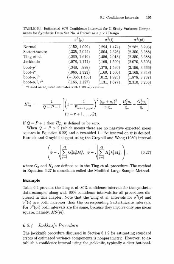
6.2 Confidence Intervals 195

TAßLE 6.4. Estimated 80% Confidence Intervals for G Study Vari an ce Compo­nents for Synthetic Data Set No. 4 Recast as a p x i Design

Normal (.152, 1.099) (.294, 1.474)Satter thwaite (.335, 2.022) (.504, 2.326)Ting et al. (.289, 1.619) (.456, 2.013)J ackknife (.078, 1.174) (.169, 1.599)

boot-p" (.348, .888) (.378, 1.536)boot- z'' (.066, 1.323) (.160, 1.506)boot-p , ia (- .068,1.435) (.012, 1.925)boot-p, i , ra (.166, 1.127) (.131, 1.677)

aBased on adjusted est imates with 1000 replications.

1Q-P-l

(2.282, 3.293)(2.350, 3.388)(2.350, 3.388)(2.070, 3.505)

(2.196, 3.366)(2.169, 3.348)(1.878 , 3.737)(2.310, 3.266)

If Q = P + 1 then H;u is defined to be zero .Wh en Q = P > 2 (which means there are no negative expected mean

squa res in Equation 6.22) and a two-sided 1 - 2a interval on 'l/J is desired ,Burdick and Gr aybill suggest using th e Graybill and Wang (1980) interval

Q

LG~k~MJ , ~ +q=l

(6.27)

where Gq and H q are defined as in the Ting et al. procedure. The methodin Equation 6.27 is sometimes called t he Modified Large Sampie Method.

Example

Table 6.4 provides the Ting et al. 80% confidence intervals for the syntheticdata example, along with 80% confidence intervals for all procedures dis­cussed in this chapter. Note that the Ting et al. intervals for (J2(p) and(J2(i) are both narrower than the corresponding Satterthwaite intervals.For (J 2(pi) both intervals are the same , because they involve only one meansqu are, namely, MS(pi).

6.2.4 Jackknife Procedure

The jackknife pro cedure discussed in Section 6.1.2 for est imating standarderro rs of est imated vari ance components is nonp arametric. However , to es­tablish a confidence interval using the jackknife , typically a distributional-

196 6. Variability

form assumption is required.l'' Usually, normality is assumed, and Stu­dent 's t distribution is employed. Thus, a 100(-y)% confidence interval foreis

where ecan be any one of the variance components and t is the (1 + 'Y)/2percentile point of the t distribution with npni - 1 degrees of freedom (seeCollins, 1970, p. 29).

For the synthetic data example , Table 6.4 provides the jackknife 80%confidence intervals. It is noteworthy that they are narrower than Sat­terthwaite and Ting et al. intervals .

6.2.5 Bootstrap Procedure

An appealing characteristic of the bootstrap algorithm is that it can beused almost automatically to obtain an approximate confidence interval,provided the number of bootstrap samples is B ~ 1000 (see Efron & Tib­shirani, 1986, p. 67). For example , a simple approach to obtaining an 80%approximate confidence interval for eis to use the 10th and 90th percentilepoints of the distribution of the Ob discussed in Section 6.1.3. More gen­erally, an approximate 100(-y)% confidence interval can be defined as the[100(1-'Y)/2]%th and [100(1 +'Y)/2]%th percentile points for Ob. (See Shao& Tu, 1995, and Wiley, 2000, for possibly better, but more complicated,approaches.) For the synthetic data example, Table 6.4 provides 80% con­fidence intervals for each of the four procedures for obtaining bootstrapsamples .

6.3 Variability of D Study Statistics

The methods and procedures discussed in Sections 6.1 and 6.2 can be ap­plied easily to D study variance components that involve nothing more thandivision of G study components by sample sizes. For the p x I design, thismeans that the standard errors for 0'2(1) and O'2(p1) = 0'2(8) are obtainedby dividing the standard errors for O'2 (i ) and O'2 (pi ), respectively, by n~ . Asimilar statement applies to the limits of the confidence intervals .

lOThe version of the jackknife discussed here is more specifically adelete-l jackknifeprocedure. Theory suggests that there may be a delete-d version that could be used toobtain nonparametrie estimates of confidence intervals for est imated variance compo­nents (see the Shao & Tu, 1995, discussion of jackknife histograms on pp . 50, 55-60) .

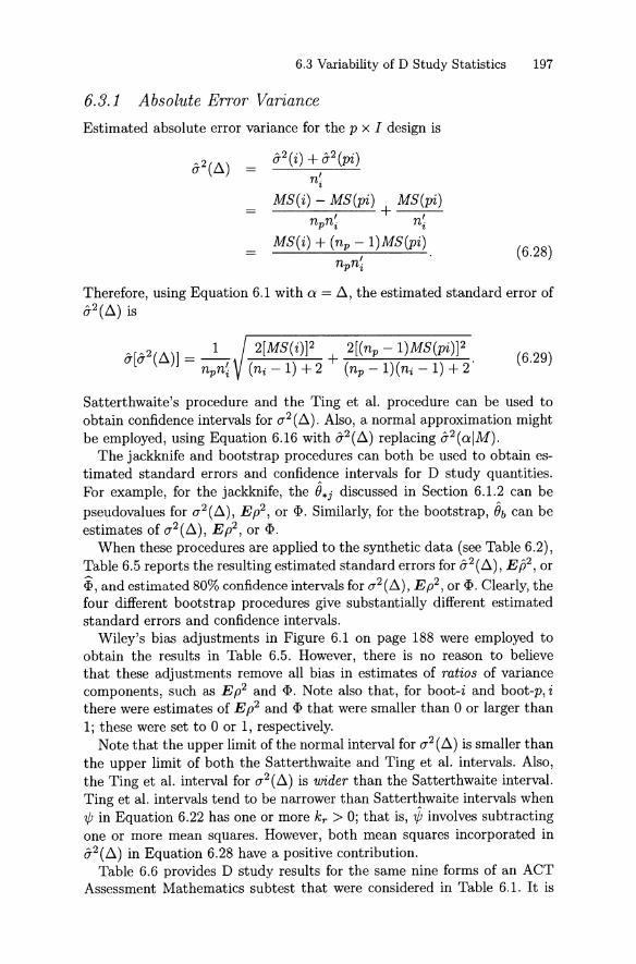
6.3 Variability of D Study Statistics 197

6.3.1 Absolute Error Variance

Estimated absolute error variance for the p x I design is

a2(i ) + a2(pi)

n~

MS (i) - MS(pi) MS(pi)-.......:-:...-~I----"'---'- + I

npni n iMS(i ) + (np - I)MS (pi)

npn~(6.28)

Therefore, using Equation 6.1 with a = .6., the estimated standard error ofa2 (.6.) is

2[MS(i)j2 2[(np - I)MS(pi)j2(n i - 1) + 2 + (np - 1)(ni - 1) + 2 .

(6.29)

Satterthwaite's procedure and the Ting et al. procedure can be used toobtain confidence intervals for a 2(.6. ). Also, a normal approximat ion mightbe employed, using Equation 6.16 with a2(.6.) replacing a2 (a IM ).

The jackknife and bootstrap procedures can both be used to obtain es­timated stand ard errors and confidence intervals for D st udy quantities.For example, for th e jackknife, t he e*i discussed in Section 6.1.2 can bepseudovalues for a2(.6.), E p2, or <P . Similarly, for the bootstrap , eb can beestimates of a2 (.6.), E p2 , or <P .

When th ese procedures are applied to the synthet ic data (see Table 6.2),Table 6.5 reports th e resulting estimated standard errors for a2(.6.) , E p2 ,or~ , and est imated 80% confidence intervals für a 2 (.6.), E p2 , or <P . Clearly, thefour different bootstrap procedures give substantially different est imatedstandard errors and confidence intervals.

Wiley's bias adjustments in Figure 6.1 on page 188 were employed toobtain the results in Table 6.5. However, there is no reason to believeth at these adjustments remove all bias in estimates of ratios of variancecomponents, such as E p2 and <P. Note also that, for boot-i and boot-p, ithere were estimates of E p2 and <P th at were smaller than 0 or larger than1; th ese were set to 0 or 1, respectively.

Note that the upper limit of the normal interval for a2 (.6.) is smaller thanthe upper limit of both the Satterthwaite and Ting et al. intervals. Also,the Ting et al. interval for a 2 (.6.) is wider than the Satterthwaite interval.Ting et al. int ervals tend to be narrower than Satterthwaite intervals when1/J in Equ ation 6.22 has one or more k; > 0; that is, .(JJ involves subtractingone or more mean squares. However , both mean squares incorp orated ina2 (.6.) in Equati on 6.28 have a positive cont ribut ion.

Table 6.6 provides D study results für the same nine forms of an ACTAssessment Mathemati cs subtest th at were considered in Table 6.1. It is

198 6. Variability

TABLE 6.5. D Study Estimated Standard Errors and Confidence Intervals forSynthetic Data Set No. 4 Recast as a p x I Design with n~ = 12, 0-2 (.0. ) = .3059,E ß2 = .729, and (f; = .672

NormalJ ackknifeboot-p"boot-i"boot-p, i a

boot-p, i , Ta

.3048

.3054

.3050

.3089

Means

.7074

.6336

.6103

.6577

.6524

.5848

.5622

.6037

Est . Standard Errors

O'2(~) E jJ2 4>

.0481

.0763 .0902 .1280

.0502 .0984 .1000

.0597 .2565 .2512

.0831 .3006 .2939

.0578 .1930 .1921

E p2 lf>

(457, .845)(.541, .876)

(.244, .368)NormalFeldtArteaga et al.bSatterthwaite (.251, .385)Ting et al. (.255, .410)Jackknife (.208, .404) (.665, .898) (.559, .889)boot-p" (.242, .372) (.595, .805) (.533, .755)boot-i" (.226, .384) (.186, .876) (.145, .838)boot-p, i a (.207, .411) (.000, .895) (.000, .855)boot- p, i, Ta (.233, .384) (.403, .829) (.343, .788)

aBased on 1000 replications; E ß2 and ~ constrained to be between 0 and 1.

bUsing the t ransformation in Equation 6.36.

evident that the empirically based estimate of O'[O'2(8}] in the next-to-the­last row is 10 times larger than the average of the normality-based estimatesin the last row. By contrast, the empirically based est imate of O'[O'2(~}] isquite elose to the average of t he normality-based est imates. This last resultis encouraging since there is good reason to believe that the score effectsfor these real data do not have a multivariate normal distribution.

6.3.2 Feldt Confidence Interval for E p2

Under normality assumptions, Burd ick and Graybill (1992) provide a de­tailed discussion of procedures for establishing confidence intervals on ratiosof variance components. One special case they consider (see pp . 128- 129) ist he two-sided 100(1 - 20:)% exact confidence interval for ( = O'2(p)/O'2(pi}

in a p x i design:

(6.30)

(6.32)

6.3 Variability of D Study Statistics 199

TABLE 6.6. D Study p x I Results for Nine Forms of ACT MathPre-Algebra/Elementary Algebra Subtest with n~ = 24 Items

Form n p MS (i) MS(pi) 0-2(<5) 0-2( ß) E p2 <I>

A 3388 85.95564 .17681 .00737 .00842 .81335 .79217B 3363 91.55995 .15167 .00632 .00745 .85719 .83580C 3458 127.28606 .14213 .00592 .00745 .83980 .80638D 3114 96.57363 .16712 .00696 .00825 .81496 .78794E 3428 63.51859 .17122 .00713 .00790 .84821 .83454F 3318 136.50134 .15989 .00666 .00837 .83346 .79925G 3257 95.13462 .17172 .00716 .00837 .80547 .77971H 3221 161.28615 .15793 .00658 .00866 .81306 .76761I 3178 94.88673 .17237 .00718 .00842 .80063 .77395

Mean .00681 .00814 .82513 .79748SD .00048 .00044 .02006 .02451Ave SEa .00004 .00039

aSquare root of the average of the squared estimated standard errors using Equa-tion 6.l.

where

L * =M p and U* = M; (6.31)

Mpi Fa:T/ p ,T/p; Mpi F 1-a:T/p ,T/p; ,

where M p = MS (p), M pi = MS(pi) , and Tl designates degrees of freedom .Obviously, as in Sect ion 6.2.3, 0: is not being used here to designat e aneffect; rather 1 - 20: is t he confidence coefficient expressed as a prop ortion .

Note t hat ( is a signal-noise ratio für n~ = 1. A genera lizability coefficientfür a test of length n~ in terms of ( is

E 2 _ n~(p - 1 + n~(

This transformation can be applied to the endpoints in Equ ation 6.30 toobtain a confidence interval for E p2. The resulting interval for E p2 is iden­tical to that derived by Feldt (1965) and is identified as such in subsequenttab les and discussion .

For the synthetic data, Mp = MS(p) = 10.2963 with 9 degrees of free­dom , and Mpi = MS(pi) = 2.7872 with 99 degrees üf freedom. Für atwo-sided 80% confidence interval , 0: = .1. Since F.9:9,99 = 1.6956 andF.l :9 ,99 = .4567, it follows t hat L* = 2.1787 and U* = 8.0888. Conse­quently, an 80% confidence interval for ( is (.0982, .5907). Transformingthese limits using Equ ation 6.32 gives (.541, .876) as an 80% interval fürE p2 .

When n p is very large, t his author's experience suggests t hat a Feldtconfidence interval für E p2 is likely to be too narrow for real test forms

200 6. Variability

based on dichotomously scored items. Consider, again, the ACT AssessmentMathematics results in Table 6.6. The range of the nine estimates of E p2

is from about .80 to .86.11 However, since n p > 3000 and ni = 24 forall forms, the degrees of freedom for both p and pi are very large, bothFa :TJp ,TJPi and F 1-a :TJp,TJPi are close to unity for moderately sized confidencecoefficients (e.g., 80%), and the resulting intervals tend to be narrower thanthe empirical data in Table 6.6 would suggest.

6.3.3 Arteaga et al. Confidence Interval [or <I>

As discussed by Burdick and Graybill (1992, p. 129) , assuming score ef­fects are normally distributed, Arteaga et al. (1982) developed the follow­ing approximate two-sided 100(1 - 20:)% confidence interval for the ratioA = (J"2(p)j[(J"2(p) + (J"2(i) + (J"2(pi)] in a p x i design.

(6.33)

where

(6.34)

and

U. _ Mi, - F1-a:TJp,ooMpMpi + (F1- a :TJp ,oo - F1-a :TJp ,TJp.)F1-a:TJp ,TJpiMi,i

p - (np -1)F1-a:TJp,ooMpMpi + F1-a :TJp ,TJiMpMi '

(6.35)with M p = MS(p) , Mi = MS(i), M pi = MS(pi), and 1] designating degreesof freedom.P

It is evident that A is <I> for the p x I design with n~ = 1. For a test oflength n~,

<1>= n~Al+(n~-l)A'

(6.36)

which is simply an application of the Spearman-Brown Formula to A.Therefore, applying the transformation in Equation 6.36 to the limits inEquation 6.33 gives a confidence interval for <1> . For the synthetic data, an80% confidence interval is (.457, 845) .

llSince the various forrns were administered to randomly equivalent groups of ex­aminees, it is unlikely that this variability in estimates is attributable to systematicdifferences in the sarnpies of persons.

12 As in Sections 6.2.3 and 6.3.2, Q does not design ate an effect here .

6.4 Same Simulation Studies 201

6.4 Some Simulation Studies

The real-data example in Tables 6.1 and 6.6 illustr ates th at normality-b asedprocedures for est imating standard errors and/or confidence intervals maynot always work weIl with dichotomous dat a. The synthet ic dat a exam­ple illustrates that different procedures for est imating stand ard errors andconfidence intervals can give quit e different results , and there is no obviousbasis for deciding which estimates are best . An investigator faced with re­sults such as those in Tables 6.2 through 6.4 may be tempted to pick modalresults or discard results that appear atypical. There is no guarantee, how­ever, that either st rategy is defensible, let along optimal.

In this section four simulation st udies are discussed th at may assist inves­tigators in choosing among methods and procedures. The first two stud­ies involve est imated G st udy variance components for th e p x i design.The next two studies involve D study statistics for the p x I design. Allbootstrap result s employ Wiley's adjustments . Wiley (2000) provides someaddit ional simulations of G study results.

6.4.1 G Study Variance Components

Two simulation studies are discussed here. The first is based on normallydistributed score effects; the oth er is based on dichotomous dat a from anactual testing program.

Normal Data

Table 6.7 provides estimated standard error and confidence interval resultsfor a simulat ion st udy using sample sizes of np = 100 and ni = 20, basedon the assumpt ion that score effects are normally distributed with variancecomponents of 0-2(p) = 4, 0-2(i) = 16, and 0-2(pi) = 64. Specifically, eachobservable person-item score was generated using the formula:

X pi = f-l + o-(p)zp + 0-(i )Zi+ o-(pi)Zpi ,

where Zp , Zi , and Zpi are randomly and independently sampled values froma unit normal distribution. (The parameter f-l is irrelevant for our pur ­poses here.) Th is dat a generation procedur e assurnes that Np -; 00 andNi -; 00. Under these assumpt ions, the actual standard errors of the est i­mated variance components are given by Equation 6.1 with mean squaresreplaced by expected mean squares.P These parameters are reported atthe top of Table 6.7.

The simulation involved 1000 t rials. Th at is, 1000 matrices of size np x niwere generated. For each t rial, the variance components were est imated.

13Degrees of freedom are not increased by two.

202 6. Variability

TABLE 6.7. Simulation of G Study Estimated Standard Errors and ConfidenceInterval Coverage with Normal Data for n p = 100, ni = 20, and 1000 Trials

Means Standard Errors

a2(p) a2(i) a2(pi) a2(p) a2(i ) a2(pi )

Par ameters 4.0000 16.0000 64.0000 1.0287 5.3988 2.0869

Empirical 4.0402 15.7535 64.0082 1.0000 5.4046 2.0326Normal 1.0338 5.3267 2.0871Jackknife 4.0402 15.7535 64.0082 1.0327 5.4893 2.0842

boot-p" 4.0395 15.7550 64.0094 1.0337 1·4966 2.0764boot-i" 4.0413 15.7536 64.0064 1.5038 5.2319 2.2956boot-p, i" 4.0407 15.7572 64.0055 2.1075 5.6380 3.6983boot-p, i, r" 4.0365 15.7532 64.0117 1.4751 5.4412 2.0869

Nominal 66.7 Percent Nominal 90 Percent

(T2(p) (T2(i) (T2 (pi) (T 2(p) (T2(i) (T 2(pi)

Normal 66.5 62.9 67.8 90.9 83.9 91.1Satterthwaite 69.6 66.6 67.4 92.1 90.1 90.8Ting et al. 67.7 66.4 67.4 91.0 89.5 90.8Jackknife 65.9 61.8 66.9 90.0 83.0 88.4

boot-p" 65.4 20.9 66.8 90.4 35.2 89.7boot-s" 84·0 60.0 71.4 98.3 82.1 92.3boot-p,ia 94·9 63.3 91·4 100.0 84.7 99·4boot-p, i, ra 84·8 62.1 67.8 98.2 83.6 90.3

aBased on 1000 replications.

Their average values are reported in the "Empirical" row in Table 6.7.The empirical standard errors in the same row are simply the standarddeviations of the 1000 estimates. The standard errors in the "Normal"row were computed using Equation 6.1, which assurnes normality.!" For aninfinitely long simulation, the par ameters , empirical estimates , and normalest imates should all be the same. The differences provide a type of yardstickfor judging the credibility of the simulation results.

For the jackknife results, each of the 1000 trials involved comput ing101 x 21 = 2121 sets of est imate d vari ance components . For each bootstrapprocedure, 1000 replications were employed for each of the 1000 t rials . Thismeans that the results for each of the boot strap procedures were based onone million p x i analyses.

14The reported values for the normal standard errors were obtained by taking thesquare root of the ave rag e of the 1000 squared standard errors.

6.4 Some Simulation Studies 203

Results th at appea r particularly ext reme to thi s author are in italies inTable 6.7. Since the simulat ion condit ions are in accord with major as­sumpt ions of the normal, Satterthwaite, and Ting et al. procedures, it isencouraging that these procedures give results that are close to the parame­te rs and nominal coverages. As predicted by theory, the normal intervals area bit too conservat ive and the Satterthwaite intervals are a bit too liberal,but not by much. Although the jackknife procedure makes no normalityassumpt ions, its results appear quit e good, at least for practical purposes.

By cont rast, the bootstrap results are mixed; it appears that:

• boot-p works weil for (J"2 (p) and (J"2(pi) ;

• boot- i works reasonably weil for (J"2(i ) and better for (J" 2(pi);

• boot-p , i works reasonably weil for (J"2(i) ; and

• boot-p , i, r works reasonably weil for (J"2(i) and quit e weil for (J"2(pi) .

Note, in particular, th at for (J"2(i) , each ofthe bootstrap procedures involv­ing sampling items (i.e., boot- i , boot-p,i , and boot-p, i, r) works reasonablyweil; however, it is not t rue th at for (J"2(p) , each of bootstrap proceduresinvolving sampling persons works weil. Since the p x i design is symmetrie,it seems sensible to conclude that at least some of the asymmet ry in theseresult s is attributable to the five-to-one ratio of the sampie sizes. Appar­ently, the applicability of the bootstrap depends to some exte nt on both thebootstrap sampling procedure employed and the pattern of sampie sizes.

Based on the results in Table 6.7, one rule that might be considered, atleast tentatively, is to use boot-p for (J"2(p) , boot-i for (J"2(i) , and boot-p, i, rfor (J" 2(pi) when it can be assumed that the score effects are approximatelyno rmal.

Nonnormal Dichotomous Data

In generalizability theory, there is often good reason to believe that scoreeffects are not normally distributed, particularly when dat a are dichoto­mous or fall into an otherwise small number of discrete categories. Forsuch data, it is risky to use a simulation such as that in Table 6.7 as a basisfor judgments about the applicability of procedur es. By way of comparison,Table 6.8 provides the result s of a simulation using dichotomous data withthe same sarnple sizes as those in Table 6.7.

Specifically, in Table 6.8 each of the 1000 tri als involved samplingn p = 100 persons without replacement from a population of size Np = 2000and n i = 20 items without replacement from a universe of size N i = 200.The 2000 x 200 dat a set is from an actual testing program.l '' Obviously,this simulation involves sampling from a finite population and universe,

15Severa l tests were concatenated to give the ent ire un iverse of 200 it ems.

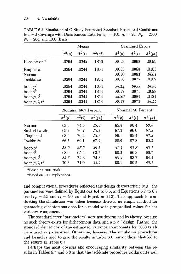
204 6. Variability

TABLE 6.8. Simulation of G Study Estimated Standard Errors and ConfidenceInterval Coverage with Dichotomous Data for n p = 100, ni = 20, Np = 2000,Ni = 200, and 1000 Trials

Means Standard Errors

a2 (p) a2 (i ) a2 (pi ) a2 (p) a2 (i ) a2 (pi )

Parameters? .0264 .0245 .1856 .0053 .0068 .0099

Empirical .0264 .0244 .1854 .0053 .0068 .0103Normal .0050 .0083 .0061Jackknife .0264 .0244 .1854 .0056 .0075 .0107

boot-p" .0264 .0244 .1854 .0044 .0033 .0056boot-i" .0264 .0244 .1854 .0057 .0071 .0098boot-p,ib .0264 .0244 .1854 .0080 .0084 .0121boot-p, i, rb .0264 .0244 .1854 .0057 .0078 .0045

Nominal 66.7 Percent Nominal 90 Percent

a2(p) a2(i) a2(pi) a2 (p) a 2(i) a2 (pi )

Normal 63.6 74.5 43.0 85.8 90.4 68.0Satterthwaite 65.2 76.7 43.2 87.2 96.0 67.3Ting et al. 63.2 76.4 43.2 86.1 95.4 67.3Jackkn ife 66.5 69.1 67.9 88.0 87.8 90.3

boot-p" 58.9 36.7 39.5 81·4 57.8 63.1boot-s" 68.9 65.4 63.7 90.3 86.3 86.7boot-p,ib 84·3 74.3 74.8 98.9 93.7 94.4boot-p, i , rb 70.8 71.0 33.0 90.1 90.5 53.1

a Based on 5000 trials.

bBased on 1000 replications.

and computational procedures reflected t his design characteristic (e.g., t heparameters were defined by Eq uations 6.4 to 6.6; and Equat ions 6.7 to 6.9used cp = .95 and Ci = .90, as did Equat ion 6.12) . This approach to con­ducting the simulation was taken because there is no simple method forgenerating dichotomous data for a model with prespecified values for t hevariance components.

The standard error "parameters" were not determined by theory, becauseno such theory exists for dichotomous data and a p x i design . Rather, thest andard deviations of the estimated variance components for 5000 trialswere used as parameters. Otherwise, however , the simulation proceduresand formulas used to give the results in Table 6.8 mirror those that led tothe results in Table 6.7.

Perhaps the most obvious and encouraging similarity between the re­sults in Tables 6.7 and 6.8 is that the jackknife pro cedure works quite well

6.4 Some Simulation Studies 205

for both normal and dichotomous data, for all three variance components.Perhaps the most obvious difference is that for the normality-based proce­dures (i.e., normal, Satterthwaite, and Ting et al.) the confidence intervalcoverage for a2(pi) is much too low for dichotomous data, and the coveragefor a 2(i) is usually too high.

The bootstrap results are mixed; it appears that:

• boot-p understates the standard errors and nominal confidence co­efficients for all variance components, although results for a 2 (p) aremuch more accurate than for a2 (i ) and a2 (pi );

• boot-i results are reasonably accurate for all variance components;

• boot-p, i results are somewhat accurate for a2 (i ) and a 2 (pi); and

• boot-p, i , r works quite weil for a2 (p) and a2 (i ), but very poorly fora2(pi) .

Clearly, conclusions based on the normal-data simulation do not all gener­alize to the dichotornous-data simulation. In particular, boot-p, i , r worksweil for a2(pi) with normal data, but very poorly with dichotomous data.

6.4.2 D Study Statistics

As noted at the beginning of Section 6.3, for the p x I design, standarderrors for 0-2(8) are obtained by dividing standard errors for 0-2(pi) byn~, and a similar statement applies to confidence interval limits for a 2 (8).Therefore, the simulation results for a2(pi) in Tables 6.7 and 6.8 can be useddirectly to obtain results for a 2 (8). Note, in particular, that the confidenceinterval coverage results for a 2 (pi) are necessarily identical to those fora 2 (t5 ).

Normal Data

Under the assumption that score effects are normally distributed, the sim­ulation results provided in Table 6.9 are for D study statistics for the p x Idesign with n~ = 20. The simulation conditions are exactly the same asthose in Table 6.7 but, of course, the statistics under consideration are dif­ferent, and there are two additional procedures: Feldt's confidence intervalfor E p2, and the Arteage et al. confidence interval for <I> .

The bootstrap estimates, standard errors, and confidence intervals forthese D study statistics employed the Wiley-adjusted bootstrap estimatesof variance components discussed in Section 6.4.1. For example, for eachbootstrap sampie, the boot-p estimate of E p2 was computed as the boot-pestimate of a2 (p) divided by itself plus the boot-p estimate of a2 (pi)/20. 16

16For E/P and ~, any bootstrap estimate smaller than 0 or larger than 1 was set too or 1, respectively.

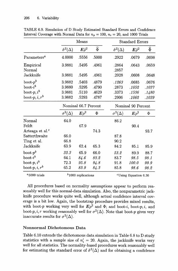
206 6. Variability

TABLE 6.9. Simulation of D Study Estimated Standard Errors and ConfidenceInterval Coverage with Normal Data for n p = 100, ni = 20, and 1000Trials

Means Standard Errors

a2(b.) E ß2 <I> a2(b.) E ß2 <I>

Parameters" 4.0000 .5556 .5000 .2922 .0679 .0698

Empirical 3.9881 .5495 .4961 .2864 .0643 .0659Normal .2857Jackknife 3.9881 .5495 .4961 .2928 .0608 .0648

boot-p'' 3.9882 .5403 .4879 .1263 .0685 .0676boot-z" 3.9880 .5295 .4790 .2873 .1052 .1037boot-p, ib 3.9881 .5110 .4629 .3373 .1536 .1480boot-p, i, rb 3.9882 .5293 .4787 .2906 .1062 .1039

Nominal 66.7 Percent Nominal 90 Percent

(]'2(b.) E p2 <I> (]'2(b.) E p2 <I>

Normal 64.0 86.2Feldt 67.9 90.4Arteaga et al.C 74.3 93.7Satterthwaite 66.0 87.8Ting et al. 66.8 90.2Jackknife 63.9 62.4 65.3 84.2 85.1 85.9

boot-p" 33.3 65.9 66.0 53.2 89.9 88.7boot-z" 64.1 84·6 83.2 83.7 98.5 98.1boot-p , i b 72.3 95.8 94·8 91.8 100.0 99.9boot-p, i , rb 65.2 83.9 84·3 85.8 98.6 98.2

a5000 trials b1000 replications CUsing Equ ation 6.36

All procedures based on normality assumpt ions appear to perform rea-sonably weil for t his normal-dat a simulation. Also, the nonparametric jack-knife proced ure works quite weil, alt hough act ual confidence interval cov-erage is a bit low. Again, the bootstrap proced ure provides mixed results,with boot-p working very weil for E p2 and <I> j and boot-i, boot-p, i, andboot-p, i , r working reasonably weil for (]'2(b.). Note that boot-p gives veryinaccurate results for (]'2 (b.).

Nonnormal Dichotomous Data

Table 6.10 extends the dichotomous data simulation in Table 6.8 to D studystatistics with a sample size of n~ = 20. Again , the jackknife works verywell for all statistics. The normality-based procedures work reasonably wellfor estimating the standard error of a2(b.) and for obtaining a confidence

6.4 Some Simulation Studies 207

TABLE 6.10. Simulation of D Study Estimated Standard Errors and ConfidenceInterval Coverage with Dichotomous Data for n p = 100, ni = 20, Np = 2000,Ni = 200, and 1000 Trials

Means Standard Errors

0-2(6 ) E ß2 <I> 0-2(6 ) E ß2 <I>

Parameters" .00946 .7596 .7363 .00047 .0411 .0452

Empirical .00947 .7544 .7308 .00048 .0418 .0459Normal .00046Jackknife .00947 .7544 .7308 .00050 .0438 .0483

boot-p'' .00944 .7501 .7264 .00026 .0360 .0385boot-i" .00944 .7468 .7229 .00046 .0478 .0517boot-p, ib .00944 .7387 .7147 .00056 .0739 .0781boot-p, i , rb .00944 .7467 .7230 .00039 .0468 .0495

Nominal 66.7 Percent Nomin al 90 Percent

a2(6) E p2 <I> a2(L\) E p2 <I>

Norm al 68.8 89.4Feldt 60.2 84.0Arteaga et al.C 64.1 87.2Satterthwaite 69.8 90.7Ting et al. 69.4 91.5Jackkn ife 69.4 68.4 68.1 90.1 90.1 89.5

boot-p'' 43.0 58.0 57.0 65.7 81.9 81.0boot-z" 65.9 67.9 67.9 88.8 90.8 90.4boot-p , i b 75.7 84 ·0 83. 9 95.0 98.8 98. 7

boot-p, i , r b 61.1 66.7 66.1 85.0 89.3 88.7

asooo trials b 1000 replications CUsing Equation 6.36

interval for a 2(L\). Confidence intervals using Feldt's procedure for E p2

and t he Art eaga et al. procedure for <I> are less accurate, but st ill probablyusable for most practi cal purposes.

For all var iance components, t he bootstrap result s using boot- p and boot­p, i are discouraging, but the boot-i results are very good. Also, the boot ­p, i , r results are quite good for the two coefficients. Clearly, the bootstrapnorm al-data simulat ion results in Table 6.9 are often not confirmed byt he bootstrap dichotomous-dat a simulations in Table 6.10. App arently, thenature of t he underlying data influences t he choice of an opt imum bootstrapprocedure.

208 6. Variability

6.5 Discussion and Other Issues

As noted at the beginning of this chapter, the subject of variability of statis­tics in generalizability theory is complicated, and there are many unan­swered questions. Also, it is evident that many procedures require exten­sive computations. For balanced designs, both GENOVA and urGENOVA(see Appendices Fand G) provide G study estimated standard errors ofthe type discussed in Section 6.1.1, and GENOVA provides D study es­timated standard errors such as those in Section 6.3.1. In addition, forbalanced designs urGENOVA provides both the Satterthwaite and Ting etal. confidence intervals for G study variance components.

Tentative Conclusions

The simulations discussed in this chapter are the only ones yet availablethat systematicaIly compare so many procedures for estimating the vari­ability of statistics in both G and D studies in generalizability theory. Thesesimulations have obvious limitations, however. They apply to single facetcrossed designs only, they involve only one pattern of sample sizes, andthey are based on only normal and dichotomous data.

Still, on balance, these tentative conclusions seem warranted:

• the jackknife procedure works quite weIl for aIl statistics and for dif­ferent types of data; this claim cannot be made for any other proce­dure;

• normality-based procedures do not work weIl for estimating standarderrors or confidence intervals for 0'2 (pi) or 0'2 (0) with dichotomousdata;

• the Ting et al. procedure works somewhat better than the Satterth­waite procedure but not so much better that the simpler Satterth­waite procedure should be abandoned entirely; and

• the Feldt and Arteaga et al. procedures work reasonably weIl forE p2 and <1>, respectively, even when score effects are not normaIlydistributed.

Admittedly, some of these conclusions involve a rather liberal interpreta­tion of "works weIl." In most cases, when standard errors and confidenceintervals are used in generalizability theory, great precision is not required .It is usuaIly sufficient that investigators not be misled by gross inaccuracies.

An important additional conclusion is that the bootstrap provides mixedresults. Sometimes boot-p, boot-i, boot-p, i, and/or boot-p, i, r works quiteweIl, but there is a notable lack of consistency across different statistics,types of data, and sample sizes. It is easy to be misled by the bootstrap,at least as it has been used here, and it is difficult to make statements

6.5 Discussion and Other Issues 209

about its genera l applicability with any great degree of confidence. Thisis unfortunat e since the bootstrap is appealing not only because of itsfreedom from distributional-form assumptions, but also because it appearsrelatively easy to generalize the bootstrap to more complicated designs (see,for example, Wiley, 2000).

M ultifacet Designs

For the most part , the norrnality-based procedures in t his chapter havebeen provided at a level of detail that makes them applicable to any bal­anced design. The confidence interval procedures for E p2 and <I> are obviousexcept ions.

The Ting et al. and Satterthwait e procedures apply to any balanced de­sign. Betebenner (1998) provides simulation results for a2(8) and a2(~)

for variou s two-facet designs. The Satterthwaite procedure is particularlyeasy to use, as discussed in Section 6.2.2. Under the assumption of nor­mally distributed score effects, there are theoreti cal reasons for concludingthat sometimes the Satterthw ait e procedure will give intervals that are tooliberal (i.e., too wide), as confirmed by the norm al-dat a simulat ions in thischa pter . However , with large numb ers of degrees of freedom, any bias inthe Satterthwaite procedure is not likely to be very big. For the single-facetsimulat ions in this cha pte r involving nonnormal data , the Satterthwaite andTing et al. coverages are largely indistinguishable (see, e.g., Table 6.8), andsometimes the Satterthwaite coverage appears slight ly better.

Extending t he jackknife to multifacet crossed designs appears straight­forward , alt hough t he computat ions may be formid able. By cont rast , it isnot unambiguously clear how to exte nd the jackknife to nest ed designs suchas p x (i :h). The essence of th e problem centers on {)- Oih and {) -rpih» If onelevel of i is to be eliminat ed from one level of h t hen the resulting designis unb alanced . If one level of i is be eliminated from each level of h, thealgorit hm does not specify which level of i should be eliminated for eachh. Note also that , when samples sizes are even moderately large, computa­tional demands for the jackknife can be excessive. One or more variationson the delete-d jackknife (see Shao & Tu, 1995) may be advisable.

Other Procedures

Sirotnik and Wellington (1977, p. 346) present ed a framework that canbe used to est imate variance components and their st and ard errors usinggenera lized symmetrie means with what they called "incidence samples ."An incidence sample refers "to the configurat ion of dat a points or entriessampled from a matrix popu lation ." Boodoo (1982) considered these proce­dures in t he specific context of generalizability theory. Stand ard errors canbe est imated using t his th eoret ical framework without revert ing to normal­ity assumpt ions, but computat ions are very complicated . The Sirotnik andWellington procedures have not been widely used in generalizability t heory,

210 6. Variability

but they may have considerable promise if their computational burden canbe overcome.

The confidence intervals discussed in this chapter are one-at-a-time in­tervals. See Burdick and Graybill (1992, pp. 18-20,51-56) for a discussionof simultaneous confidence intervals. Under normality assumptions, Khuri(1981) developed an elegant but complicated procedure for simultaneousconfidence intervals for balanced random models , and Bell (1986) discussedthe Khuri procedure in the specific context of generalizability theory. TheBonferroni inequality applied to one-at-a-time intervals is a simpler ap­proach that often leads to shorter intervals. If Q intervals with a commoncoverage probability are to be established such that

Pr(Lq ~ 'ljJq ~ Uq) = 1 - 2a (q = 1, ... ,Q),

then the Bonferroni inequality states that

2:: 1 - Q(2a).

(LQ s 'ljJQ s UQ)]

(6.37)

So, if an investigator wants a simultaneous coverage probability of at leastSPr for Q intervals , then each of the individual intervals should use

1- SPra=

2Q

which gives an individual coverage probability of

For example, if it is desired that the overall coverage be SPr = .80 for Q = 3intervals, then individual intervals should use a = .0333, which gives anindividual coverage probability of Pr = .9333.

"Achilles Heel" Argument

It has almost become conventional wisdom to believe that the variabilityof estimated variance components is the "Achilles heel" of generalizabilitytheory. Commenting on this, Brennan (2000a, p. 8) states:

Because a generalizability analysis focuses on estimating vari­ance components, the credibility of any conclusions rests onthe extent to which estimated variance components are reason­ably accurate refiections of the parameters. However, it is wellknown that estimated variance components can be quite un­stable when the number of conditions of measurement is small,which is often the case.

6.6 Exercises 211

To the extent that the "Achilles heel" argument is valid , it ap­plies, of course, not only to (generalizability) theory but also toany variance components model. Such models are very preva­lent in statistics, and investigators do not discard them simplybecause some of the est imated parameters may contain sizablerandom error. In th is sense, it is easy to exaggerate the impor­tance of the "Achilles heel" argument , at least relative to whatis accepted practice in other areas of statistical inference.

More importantly, however , the "Achilles heel" argument , asit is usually stated, can be misleading. The argument typicallyfocuses on est imated variance components for single condit ionsof measurement , whereas decisions about examinees are madewith respect to mean or total scores over all sampled condi­tions of measurement. . .. These can be, and often are, quitesmall even when the standard errors for single condit ions ofmeasurement are relat ively large.

Even with (these) caveats . .. , the "Achilles heel" argumentis probably more helpful th an harmful. It properly encouragesinvestigators to pay attention to sampling error, and it providesa strong although indirect challenge to investigators to gatheras much data as possible. After all, th e ultim ate solution tolarge standard errors is the collect ion of more dat a, not simplybetter estimat ion procedures.

It is easy to be discouraged by the complexit ies or inaccuracies of variousmethods discussed in this chapter, and the occasional inconsistent resultsacross methods. Still , in generalizability theory it is almost always advis­able to employ one or more methods to est imate the variability of st atisticsused to make important decisions, even if the methods chosen are less thanoptimal. The message of this chapter is that results should be interpretedwith caut ion, not th at th e topic of variability in est imates should be disre­garded.

6.6 Exercises

6.1* Verify the result for a- [a-2 (~ ) 1 reported in Table 6.2.

6.2* Verify the 80% Satterthwaite confidence interval for a2(~) reportedin Table 6.2.

6.3 Verify the lower limit of the Ting et al. confidence interval for a 2 (p)in Table 6.4.

6.4 Given the results for the p x i design in Table 6.2, what is an 80%confidence interval for a( ß ) if the D study uses the I :p design with

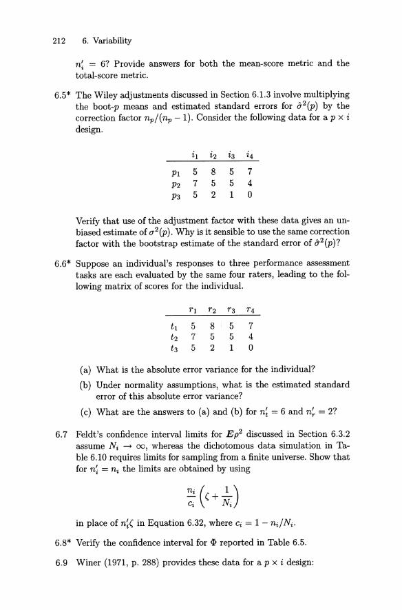
212 6. Variability

n~ = 6? Provide answers for both the mean-score metric and thetotal-score metric.

6.5* The Wiley adjustments discussed in Section 6.1.3 involve multiplyingthe boot-p means and est imate d standard errors for a2(p) by thecorrection factor np/ (np - 1). Consider the following data for a p x idesign.

PI 5 8P2 7 5P3 5 2

5 75 41 0

Verify that use of the adjustment factor with these data gives an un­biased estimate of a 2 (p). Why is it sensible to use the same correctionfactor with the bootstrap estimate of the standard error of a2(p)?

6.6* Suppose an individual 's responses to three performance assessmenttasks are each evalua ted by the same four raters, leading to the fol­lowing matrix of scores for the individual.

t 1 5 8 5 7t2 7 5 5 4t3 5 2 1 0

(a) What is the absolute error variance for the individual?

(b) Under normality assumptions, what is the estimated st andarderror of this absolute error variance?

(c) Wh at are the answers to (a) and (b) for n~ = 6 and n~ = 2?

6.7 Feldt's confidence interval limits for E p2 discussed in Section 6.3.2assurne Ni -+ 00, whereas the dichotomous data simulation in Ta­ble 6.10 requires limits for sampling from a finite universe. Show thatfor n~ = ni the limits are obtained by using

in place of n~( in Equation 6.32, where Ci = 1 - ni/Ni.

6.8* Verify the confidence interval for <I> reported in Table 6.5.

6.9 Winer (1971, p. 288) provides t hese data for a p x i design:

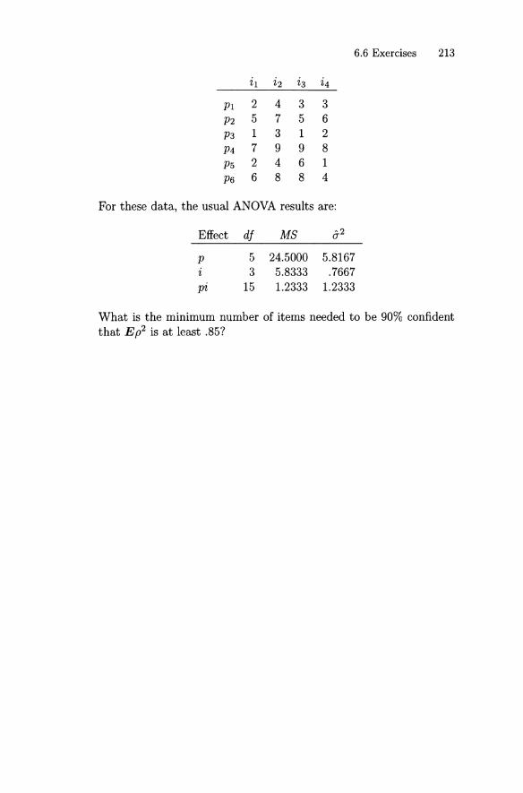
6.6 Exercises 213

i1 i2 i3 i4

Pl 2 4 3 3P2 5 7 5 6P3 1 3 1 2P4 7 9 9 8P5 2 4 6 1P6 6 8 8 4

Für these data, the usual ANOVA results are:

Effect df MB 6"2

P 5 24.5000 5.81673 5.8333 .7667

pi 15 1.2333 1.2333

What is th e minimum number of items needed to be 90% confidentthat E p2 is at least .85?

7Unbalanced Random Effects Designs

To t his point , our discussion of generalizability theory has been restrictedto balanced designs. Doing so substantially decreases a number of statist icalcomplexit ies, and even some concept ual ones. In pract ice, however, gener­alizability analyses with real data are often cha racterized by unb alanceddesigns. Unbalanced random effects designs are the subject of t his chapte r.Unbalanced mixed effects designs are t reated using multivariate generaliz­ability theory, which is discussed in Chapters 9 to 12.1 The discussion hereof unb alanced random effects designs is relevant for bot h univariat e andmultivariate generalizability theory.

There is a vast stat istical literat ure on esti mating variance componentswith unb alanced random effects designs. Most of thi s literature is exten­sively reviewed by Searle et al. (1992), with Searle (1971, Chap . 10) pro­viding an earlier treatment. Jarjoura and Brennan (1981) and Brennan(1994) provide brief summaries. One reason the literature is so extensiveis that there are numerous, and sometimes conflicting, perspectives on thesubject . As vast as the literature is, however, for our purposes it is limitedin one respect-it deals almost exclusively with G st udy issues, although,of course, discussions in stat ist ical literature do not use such terminolo gy.

In this chapte r the est imation of G study variance components is treatedprim arily in terms of one part icular method called t he analogous-A N OVA

1 In multivar iat e generalizability t heory, t he fixed effects in a mixed model play therole of multiple depend ent variabl es, and t here is a random effects design (balancedor unbalan ced) associated wit h each variable. Therefore, in generalizability t heory weseidom need to t reat unbal anced mixed models in t he convent iona l st atistical sense.

216 7. Unbalanced Random Effects Designs

procedure. General equations are provided, along with results and illustra­tions for several G study designs. Matters are even more complicated forD studies, and general procedures applicable to any unbalanced D studydesign are unknown. Consequently, in this chapter estimators of error vari­ances and coefficients are derived and illustrated for several, frequentlyencountered unbalanced D study designs.

7.1 G Study Issues

It is important to recall that the estimation problems induced by unbal­anced designs do not affect the definition of G study variance components.That is, the variance components that characterize the universe of admissi­ble observations are blind to the complexities of estimating random effectsvariance components, and the definitions discussed in Section 3.4 still apply.

In this book, to estimate random effects variance components for bal­anced designs we have employed primarily the ANOVA procedure, whichinvolves solving the simultaneous linear equations that result from equat­ing mean squares with their expected values. Since sums of squares arelinear combinations of mean squares, the same estimators of variance com­ponents would be obtained by equating sums of squares with their expectedvalues. Similarly, since the T terms discussed in Section 3.3 are linear com­binations of sums of squares (and mean squares), the same estimators ofvariance components would be obtained by equating T terms with theirexpected values. Whichever of these sets of statistics is used, the resultingestimators of variance components are unbiased; indeed, they are calledbest quadratic unbiased estimators (BQUE).

Mean squares, sums of squares, and T terms are examples of quadraticforms, that is, statistics that involve squared values of the observations. Anumber of other quadratic forms might be employed to estimate variancecomponents with balanced designs, but a great many of them lead to thesame estimators as those obtained from the ANOVA procedure. For ex­ample, with the p x i and ni = 2, the covariance of person mean scores isidentical to the estimator of a 2(p) obtained from the ANOVA procedure.

The fact that many quadratic forms give the same estimators of variancecomponents with balanced designs is not a statistical virtue per se, but itdoes provide a sense of security that evaporates when unbalanced designsare encountered. For unbalanced designs, it is rare for different quadraticforms to lead to the same estimators of variance components, even whenthe various estimators are unbiased. Furthermore, many properties of theestimators are usually unknown. For unbalanced designs, then, the prin­cipal problem is not obtaining estimators of variance components; rather,the principal problem is that there are many estimators and no obviousstatistical basis for choosing among them.

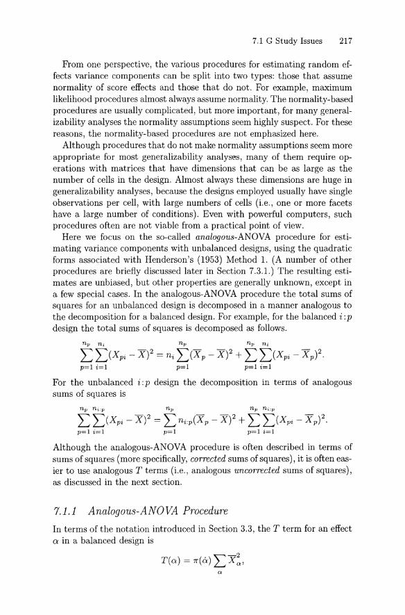
7.1 G Study Issues 217

From one perspective, the various procedures for est imat ing random ef­fects variance components can be split into two types: those that assumenormality of score effects and those th at do not . For example, maximumlikelihood procedures almost always assume normality. The normality-basedprocedures are usually complicated, but more important , for many general­izability analyses the normality assumpt ions seem highly suspect . For thesereasons , the normality-b ased procedures are not emphasized here.

Although procedures that do not make normality assumptions seem moreappropriate for most generalizability analyses, many of them require op­erations with matrices that have dimensions that can be as large as thenumb er of cells in the design. Almost always these dimensions are huge ingeneralizability analyses, because the designs employed usually have singleobservat ions per cell, with large numbers of cells (i.e., one or more facetshave a large number of condit ions). Even with powerful computers, suchprocedures often are not viable from a practical point of view.

Here we focus on the so-called analogous-ANOVA procedure for est i­mating variance components with unbalanced designs, using the quadr ati cforms associated with Henderson's (1953) Method 1. (A number of otherprocedures are briefly discussed later in Section 7.3.1.) The resulting est i­mates are unbiased, but other properti es are generally unknown , except ina few special cases. In the analogous-ANOVA procedure the total sums ofsquares for an unbalanced design is decomposed in a manner analogous tothe decomposition for a balanced design. For example, for the balanced i :pdesign the total sums of squares is decomposed as folIows.

n p n i n p n p ni~~ - 2 ~- - 2 ~~ - 2L...J L...J(Xpi - X) = ni L...J (X p - X) + L...J L...J(Xpi - X p ) .

p= l i=l p=l p=li= l

For the unbalanced i: p design the decomposition in terms of analogoussums of squares is

Although the analogous-ANOVA procedure is often described in terms ofsums of squares (more specifically, corrected sums of squares), it is often eas­ier to use analogous T terms (i.e., analogous uncorrected sums of squares),as discussed in the next sect ion.

7.1.1 Analogous-ANOVA Procedure

In terms of th e notation introduced in Section 3.3, th e T t erm for an effect0: in a balanced design is

218 7. Unbalanced Random Effects Designs

where 7I"(ä) is the product of the sample sizes for the indices not in o, andthe summat ion is over all of the indices in o. This means that each of theX~ terms is multiplied by the same constant 7I"(ä) , which is the numberof observations involved in computing each mean X 0:' For an unbalanceddesign, however , the multiplier is not necessarily a constant. Consider , forexample, the unbalanced p x (i :h) design in which the number of itemswithin each level of h (ni:h) need not be the same. For T(h) in this design,X h is based on npni:h observations , which is not a constant for all levels ofh.

So-called analogous T terms are defined as

(7.1)

where

n<:> is the total number of observations for a given level of o,

e is the set of all indices that are not in o ,

a c means all of the indices in the design, and

the last term is a frequently used computat ional formula.

So, for example, for the unbalanced p x (i :h) design,

It is important to note th at X<:> in Equation 7.1 is defined as a sumdivided by the total number of observations that are summed. So, for ex­ample, for the unbalanced p x (i :h) design,

_ n h n i :h

LLXpihX - h=l i=l

P - n h

Lni:hh=l

Th at is, X p is the sum of all the observations for a level of p divided bythe total number of such observations. By contr ast , X p is not defined as

which is the average over levels of h of the average over levels of i. Ofcourse, these two definitions are equivalent for balanced designs.

Estim ating random effects variance components using analogous T termsinvolves these steps:

(7.2)

7.1 G Study Issues 219

1. obtain the expected value of each T term with respect to fl2, thevariance components, and their multipliers (i.e., coefficients) , and

2. use matrix procedures, or traditional algebraic procedures, to esti­mate the variance components.

Both steps are usually tedious, but obtaining the coefficients of fl2 and thevariance components is considerably simplified by general results discussedby Searle (1971, p. 431) and Searle et al. (1992, p. 186).

In our notation, the coefficient of fl2 in the expected value of every Tterm is simply

where n+ is the total number of observations in the design.e The coeffi­cients of the variance components are often more complicated, however. Ingeneral, the coefficient of (1'2(0:) in the expected value of the T term for ßis

(7.3)

where

, is the set of all indices in 0: that are not in ß (if ß = u; then,= 0:);

nß'Y is the total number of observations for a given combination oflevels of ß and , ; and

nß is the total number of observations for a given level of ß (note

that nß = L'Y nß'Y)'

One useful special case of Equation 7.3 is

(7.4)

where n" is the total number of observations for a given level of 0:. Notealso that

(7.5)

and(7.6)

where w is the effect associated with all the indices in the design.It is important to note that derivation of the k terms given by Equa­

tions 7.2 to 7.6 assumes that the sample sizes are uncorrelated with the

2The coefficient k in this section should not be confused with the coefficients k q andk; in Section 6.2.3 .

220 7. Unbalanced Random Effects Designs

TABLE 7.1. Analogous T Terms for Unbalanced i :p Design

Effect df T SS-2

T(p) - T(J.L)p np -1 'Epni:pXp

i:p n+ -np 'Ep 'Ei X;i T(i:p) - T(p)

Mean(J.L)-2

1 n+X

Note. n+ = 'Ep ni:p'

effects in the linear model for the design. Also, it is assumed that the sam­pie sizes, and sampie size patterns for unbalanced facets, are the same overreplications.

In the following sections, the analogous-ANOVA procedure is illustratedfor the unbalanced i :p design, the unbalanced p x (i: h) design, and thep x i design with missing data. Appendix E provides results for the unbal­anced i: h:p and (p: c) x i designs.

7.1.2 Unbalanced i :p Design

Table 7.1 provides the T terms for the unbalanced i :p design. Consider thecoefficient of (72(p) in the expected value of T(J.L). Using Equation 7.4 witha=p,

As another example, consider the coefficient of (72 ( i: p) in the expected valueof T(p). To obtain this coefficient, use a = i:p and ß = p in Equation 7.3:

Note that npi is the number of observations in each pi combination, whichis necessarily one, because this design has only a single observation for eachcell. Derivation of the other coefficients is straightforward.

The full set of expected T terms is

where

ET(p)

ET(i:p)

ET(J.L)

n+J.L2+ np(72(i:p) + n+(72(p)

n+J.L2+ n+(72(i:p) + n+(72(p)

n+J.L2+ (72(i:p) + Ti (72 (p),(7.7)

(7.8)

Note that ri = ni for a balanced design. That is why the subscript i isattached to r .

Since there are an equal number of equations (the three ET terms) andunknowns (J-L2 and the two variance components), matrix procedures canbe used to obtain estimates of the variance components; the ET termsare simply replaced with computed numerical values. Alternatively, con­ventional algebraic procedures can be employed to express estimators ofthe variance components in terms of analogous T terms, which gives

T(i:p) - T(p)

n., -np

T(p) - T(J-L) - (np - 1)&2(i:p)

(7.9)

(7.10)

Estimators can also be obtained in terms of analogous sums of squares oranalogous mean squares. Analogous sums of squares are obtained by usinganalogous T terms in the usual formulas for sums of squares. Analogousmean squares are analogous sums of squares divided by their degrees offreedom."

Using the expected T terms in Equation Set 7.7 it is easy to derive theexpected values of the analogous mean squares. For example,

EMS(p)ET(p) - ET(f.L)

np -1

3For a nested main effect, the degrees of freedom equals the sampie size associatedwith all indices in the effect minus the sampie size associated with the nesting indices inthe effect . The degrees of freedom for an interaction effect is the product of the degreesof freedom for the main effects that make up the interaction effect.

222 7. Unbalanced Random Effects Designs

(n+ - n+)J1-2 + (np - 1)(j2(i:p) + (n+ - Ti)(j2(p)n p -1

wheren -T't _ + t

t - np

- 1

Similarly,

EMS(i:p)

=

ET(i :p) - ET(p)

n+ -np

(n+ - n+)J1-2 + (n+ - np)(j2(i:p) + (n+ - n+)(j2(p)n+ -np

It follows immediately that the estimators of the variance components interms of analogous mean squares are

a2(p) = [MS(p) - MS(i:p)] jti

a2(i :p) = MS(i:p).

(7.11)

(7.12)

The estimators are unbiased, as are all analogous-ANOVA estimators. Inaddition, for this design, Henderson's (1953) Methods 1 and 3 give the samedecomposition of the sums of squares. Also, assuming effects are normallydistributed, Searle et al. (1992, Chap. 4) discuss other properties of theseestimators."

Table 7.2 provides a small synthetic data example that illustrates thecomputation of estimated variance components for the unbalanced i :p de­sign. Additional aspects of this example are discussed later in Section 7.2.

7.1.3 Unbalanced p X (i: h) Design

Table 7.3 provides degrees of freedom and T -terms for each effect in the un­balanced p x (i: h) design, and Table 7.4 provides all of the coefficients forthe expected values of the T terms for this design. Consider, for example,the coefficient of (j2(h) in the expected value of T(p) for the unbalancedp x (i: h) design. To obtain this coefficient, use a = hand ß = p in Equa­tion 7.3. Since a contains only h, and h is not one of the indices in ß, itfollows that 'Y = h. Therefore,

4 At the beginning of this chapter it was noted that the properties of analogous­ANOVA estimators of variance components are generally unknown for unbalanced de­signs , except for a few special cases . The unbalanced i :p design is one such exception.

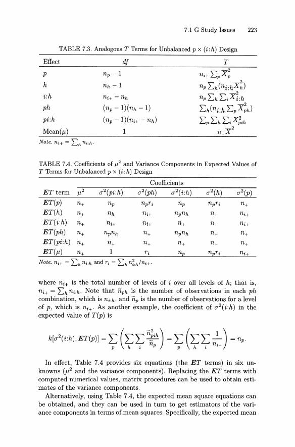
7.1 G Study Issues 223

TABLE 7.3. Analogous T Terms for Unbalanced p x (i: h) Design

Effeet

p

h

i :h

ph

pi:h

Mean(J.L)

Note. ni+ = L:h ni :h'

df

(np - l )( nh - 1)

(np - l )( n i+ - n h)

1

T

TABLE 7.4. Coefficients of J-L2 and Variance Components in Exp ected Values ofT Terms for Unbalanced p x (i :h) Design

Coefficients

ET (p) n + n p n pTi n p npTi n +

ET (h) n + nh n i+ n pn h n+ n i+

ET (i :h) n + n i+ ni+ n + n + ni+

E T (ph) n + npnh n + npnh n + n +

ET(pi :h) n + n+ n + n + n + n+

ET(J.L ) n+ 1 Ti np n pTi n i+

Note. ni+ = L:h ni :h and Ti = L:h n;:h/ni+'

where ni+ is t he tot al numb er of levels of i over all levels of h: t hat is,ni+ = L:h n i :h' Note that nph is t he numbe r of observat ions in eaeh pheombinat ion, which is n i :h, and n p is the number of observat ions for a levelof p, which is n i+ ' As anot her example, t he eoefficient of a 2(i :h) in theexpected value of T(p) is

k[a2(i :h),ET(p)] = L (LL n~ih ) = L (LL f-)= np'p hi p p hi H

In effeet, Table 7.4 provides six equat ions (the E T terms) in six un­knowns (J.L2 and the varianee eomponents). Replacing the E T terms wit heomputed numerieal values, matrix proeedures ean be used to obtain est i­mates of t he varianee eomponents.

Altern atively, using Table 7.4, t he expeeted mean square equat ions eanbe obtained, and t hey ean be used in turn to get est imato rs of t he vari­anee eomponents in te rms of mean squares. Specifieally, t he expected mean

224 7. Unbalanced Random Effects Designs

TABLE 7.5. Synthetic Data Example for Unbalanced p x (i:h) Design

12345678

Mean

4 52 12 41 33 31 23 5o 1

2 3

3 3 5 42 3 1 44 7 6 5545 56 7 5 75 6 4 46 8 6 71 204

4 5 4 5

5 74 68 74 58 95 67 87 8

6 7

4.50 3.75 6.00 4.5001.50 2.50 5.00 2.8753.00 5.50 7.50 5.3752.00 4.75 4.50 4.0003.00 6.25 8.50 6.0001.50 4.75 5.50 4.1254.00 6.75 7.50 6.2500.50 1.75 7.50 2.875

2.50 4.50 6.50 4.500

.4800

.96561.4906

.79002.29001.41561.04254.3856

1.6075

np = 8 ni+ = 8 ri = 3.0000 nh = 2.6667

Effect df T MS

phi:hphpi :hf.L

7 1390.02 1424.05 1440.0

14 1564.535 1610.0

1 1296.0

13.428664.00003.20003.3214

.8429

1.20142.9161

.2946

.9913

.8429

square equations are

EMS(p)

EMS(h)

EMS(i:h)

EMS(ph)

EMS(pi:h)

a2(pi:h) + ri a2(ph) + ni+ a2(p)

= a2(pi:h) + ti a2(ph) + npa2(i:h) + npti a2(h)

= a2(pi:h) + npa2(i:h) (7.13)

= a2(pi:h) + ti a2(ph)

= a2(pi:h),

where

andn, - r't. - t+ t

t - nh- 1

Note that these values of ri and t, are different from those for the i :pdesign.

Using Equation Set 7.13, est imators of the variance component s in termsof mean squares are

&2(p) [MS(p) - riMS(ph)jti + h - ti)MS(pi:h)jti]/ni+

&2(h) = [MS(h) - MS( i :h) - MS(ph) + MS(pi :h)]/npti

a-2 (i :h)

a-2 (ph)

a-2(pi :h)

[MS(i: h) - MS(pi: h)]jnp

[MS(ph) - MS(pi:h)]jt i

MS(pi :h) .

7.1 G St udy Issues 225

(7.14)

The result s in Equation Set 7.14 were first report ed by Jarjoura and Bren­nan (1981).

Table 7.5 provides a small synthetic data example of t he unb alancedp x (i :h) design." Certain aspects of t his example are discussed lat er whenwe consider D st udy issues for unbalanced designs.

7.1.4 Missing Data in the p x i Design

The unb alanced i :p and p x (i: h) designs described in Sections 7.1.2 and7.1.3, respectively, are unbalanced with respect to nesting. By cont rast ,suppose some dat a are missing at random from the p x i design. Let np bet he number of nonmissing observations for person p and ni be the numb erof nonmissing observations for item i . For t his design, Tab le 7.6 providesformulas for degrees of freedom, analogous T terms, and sums of squares.Note that the degrees of freedom for t he pi effect is not the product of t hedegrees of freedom for t he p and i effects. Rather, the degrees of freedomfor pi is the total number of degrees of freedom (n+ - 1) minus t he degreesof freedom far p and i. In this sense, the pi effect is to be interpreted as aresidua l effect.

T he expected T-term equations are

where

E T (p)

E T (i )

E T (pi )

ET(f.L )

n+f.L2 + np(J'2(pi) + np(J'2(i) + n+(J'2(p)

n+f.L2+ nw2(pi) + n+(J'2(i) + nw2(p)

n+f.L2 + n.,(J'2 (pi) + n+(J'2(i) + n+(J'2(p)

n+f.L2+ (J'2(pi) + r p(J'2(i) + rw2(p),

(7.15)

and

Given t hese expected T-term equations, it is st raightforward to showthat t he expected mean squares are

5T he d at a are from Rajaratnam et a l. (1965), a lt hough the analysis here is di fferentfrom theirs.

226 7. Unbalanced Random Effects Designs

TABLE 7.6. Analogous T Terms for p x i Design with Missing Data

Effect df T SS-2

T(p) - T(p.)p np -1 r, npXp_-2

T(i) - T(p.)i ni -1 I:i niX i

pi n+ - np - ni + 1 I:p I:i X;i T{pi) - T(p) - T(i) + T(p.)-2

P. 1 n+X

EMS(p)

EMS(i)

EMS(pi)(7.16)

Note that there is a nonzero coefficient for each of the three variance com­ponents in each of the expected mean squares. By contrast, for designs thatare unbalanced with respect to nesting, only, E MS (ß) involves solely thosevariance components that include all of the indices in ß.

Because the expected mean square equations in Equation Set 7.16 arequite complicated, expressions for estimators of the variance componentsin terms of mean squares are quite complicated, too . Consequently, it issimpler to express estimators of the variance components with respect toT terms. Letting

and

(7.17)

the estimators of the variance components are

Ap[T(pi) - T(p)] + AdT(pi) - T(i)] - [T(pi) - T(p.)]

n+ - r p - ri + 1

T(pi) - T( i) A 2( ')- (7 pt

n+ - ni

T(pi) - T(p) A2( ')-(7 pt],

n+ -np

These estimators were reported by Huynh (1977) based on somewhatmore general equations in Searle (1971, p. 487). Table 7.7 provides a simplesynthetic data example from Huynh (1977) that illustrates the computationof estimates of variance components for a p x i design with missing data.

7.2 D Study Issues 227

TABLE 7.7. Huynh (1977) Example of Missing-Data p x i Design

It ems

p 1 2 3 4 5 6 n p X p Effect df T (j2

1 1 1 1 1 0 1 6 .8311 27.8000 .0473

2 1 0 1 1 1 1 6 .83 P

3 1 1 1 0 0 5 .605 24.7432 .0117

4 0 1 0 1 4 .50pi 42 37.0000 .1840

5 1 0 1 0 4 .50 J..L 1 23.2034

6 1 1 1 1 0 1 6 .83 n p 127 0 1 0 0 4 .258 0 1 1 1 1 5 .80 n i 6

9 1 1 0 1 0 5 .60 n + 59

10 0 0 0 0 4 .00 Tp 9.949211 1 1 1 1 1 1 6 1.00 Ti 5.067812 0 0 0 1 4 .25

iii 4.7682n i 9 8 10 11 10 11 59

The analogous-ANOVA procedure can also be used with more compli-cated missing-data designs. The computat ions are more complex, but thebasic procedure is the same. It is almost always easier to work with T termsand t heir expected values rather than with SS or MS terms.

7.2 D Study Issues

T he analogous-ANOVA procedure for estimating variance components takesinto account the missing data pattern in obtaining the est imates, but theest imate s t hemse lves are est imates of populationjuniverse parameters t hatare defined in such a way that they do not depend on whether data aremissing in obtaining the est imates. So, for example, for the p x (i: h) design ,whet her t he G study is balanced or unbalanced , for the universe of admis­sible observations t he definition of a 2 (p) is EI/; , the definit ion of a 2 (h) isEI/~ , and the definit ion of a 2 (i :h) is E I/; h. Similarly, for t he universe ofgeneralization, t he definition s of t he variance components do not dependon whether t he D study design is balanced or unbalanced . It follows t hatthe occurrence of missing data in the D st udy has no effect on universescore variance. Error vari ances, however , are affected by whether or notthe D study design is balanced.

Suppose the G study design is unbalanced, and consider several possi­biliti es. First, the D st udy might use a balanced design. In this case , theest imate s of the vari ance components from the unbalanced G study areused in exact ly the same way as discussed in Chapters 4 and 5. Second ,

228 7. Unbalanced Random Effects Designs

the D study might use the same sample sizes and sample size patterns asin the G study; that is, decisions might be based on the same data as inthe G study. In this case, error variances are affected by the unbalancedcharacteristics of the G study. Third, the D study might use an unbalanceddesign with sample sizes and/or sample size patterns different from those inthe G study. In this case, error variances will be affected by the unbalancedcharacteristics of the D study.

In generalizability theory, then, unbalanced D study designs often involveconceptual and statistical complexities over and beyond those addressedin statistical treatments of variance components (e.g., Searle, 1971, andSearle et al., 1992). In effect, such treatments consider G study issues,only. By way of illustration, a few of the complexities arising from theunbalanced characteristics of several D study designs are considered in thefollowing sections. The only designs treated explicitly are the unbalancedI:p, p x (I:H), (P:c) x I, and p x I designs.

For balanced designs, as discussed in Chapters 4 and 5, it is possible toprovide relatively simple, general formulas for obtaining D study results forany design. For unbalanced designs, formulas are generally much more com­plicated. Often it is necessary to derive results for the specific design andcircumstances under consideration, as illustrated in the following sectionsand in the exercises at the end of this chapter.

7.2.1 Unbalanced I: p Design

By definition, absolute error is the difference between the observed anduniverse score for an object of measurement. For the unbalanced I: p design,assuming the G and D study sample sizes are the same,

The expected value of ~~ is absolute error variance:

7.2 D Study Issues 229

where i =I i' , The expected values of the eross-product terms are all zero,and the expected value of eaeh squared term is the same. It follows that

whieh clearly depends upon the ni:p' Reeall that (J2( i:p) = Evt,p, and as­sume that the distribution of the ni :p in the population mirrors that in thesample. It follows that

2- L [(J2(i:P)]np p nt :p

(J2( i:p)

ni

where ni is the harmonie mean of the ni:p; namely,

(7.18)

(7.19)

The error varianee (J2(ß) in Equation 7.18 was derived without distin­guishing between G and D study sample sizes. However, they need not beequal. The variance component (J2 (i :p) ean be estimated using the G studysarnple sizes, and it ean be used in Equation 7.18 along with the harmoniemean for the D study sample sizes n~ .

An alternative perspeetive on (J2(ß) is to view it as the average of theeonditional absolute error varianees, in the manner diseussed in Seetion 5.4.For the I :p design, conditional absolute error variance for a person is simplythe variance of the mean of the item scores for the person. Consequently,assuming the G and D study sample sizes are the same,

(7.20)

This equation eannot be simplified using an harmonie mean beeause bothvar(Xpilp) and ni:p eould vary for eaeh person.

For balaneed I :p designs, using ANOVA estimates of varianee eompo­nents in Equations 7.18 and 7.20 gives the same estimate of absolute er­ror varianee . This equality does not neeessarily hold for unbalaneed de­signs, however. Consider again the synthetie data example in Table 7.2 onpage 221. Using Equation 7.18, a-2 (ß ) = 1.8071/3 .9130 = .4618, but usingEquation 7.20, the reader ean verify that the average of the conditionalabsolute error varianees is a-2 (ß ) = .5293.

For the unbalaneed I :p design, Op = ß p, as it does for the balaneeddesign. Viewing a generalizability coefficient as the ratio of universe score

230 7. Unbalanced Random Effects Designs

variance to itself plus relative error variance, we obt ain different est imatesdepending on whether we use Equation 7.18 or 7.20. For the synthet ic datain Table 7.2, using Equation 7.18 gives Eß2 = .525, and using Equation 7.20gives E ß2 = .49l.

A generalizability coefficient can be viewed also as the rat io of universescore variance to expected observed score variance. From thi s perspective,the invest igator might est imate a generalizability coefficient as the ratio ofa2 (p) to the variance of the observed mean scores for persons:

where

- 2 -2L pXp -npX

np -1(7.21)

(7.23)

_ 1 n i:" _ 1 n,, _

x; = -LXPi and X = - LXp- (7.22)ni :p i =l np p=l

It is important to recognize that S 2(p) in Equation 7.21 is not as simplea st atistic as it is for balanced designs. Complexities arise for two relat edreasons: the mean scores for different persons can be based on differentnumbers of items ; and the grand mean X is an unweighted average of theperson mean scores, not L p L i X pdn+ .

It can be shown that

( 2) n (J"2(i ·p)E L pX p = np/i? + np(J"2 (p) + p ni · ,

andE (X2) = J.L2 + (J"2(p) + (J"2 (i.~p ) . (7.24)

np npni

It follows that the expected value of the observed score variance in Equa­tion 7.21 is6

ES2( ) 2( ) (J" 2(i:p)p = (J" p + .. .ni

(7.25)

The form of the expected value of the observed score variance in Equa­tion 7.25 clearly indicates that it is (J"2(p) plus the absolute error variancein Equation 7.18. Consequently, with respect to parameters

Ep2 = (J"2(p) = (J"2(p)

ES2(p) (J"2(p) + (J"2 (~) '

where (J"2(~) is given by Equat ion 7.18. This equality in terms of parametersdoes not necessarily hold for the estimators that have been discussed here,

6 As noted pr eviously, Cronbach et al. (1972) and Bren nan (1992a) des ignate expectedobserved score variance using E q 2(X ). In t his boo k, however , ES2(p) is used for ex­pected observed score varian ce, which simplifies some notational conventions, especiallyin Ch ap ters 9 to 12.

7.2 D Study Issues 231

however. Specifically, replacing the mean-square estimators of O'2 (p) and

O'2 ( i:p) (see Equations 7.11 and 7.12, respectively) in Equation 7.25 doesnot lead to the observed score variance in Equation 7.21. For example, forthe synthetic data in Table 7.2 on page 221, the variance of the observedperson mean scores is .9428, which leads to Eß2 = .541 using Equation 7.25,whereas Eß2 = .525 using Equation 7.18 for a-2(~).

In short, for the unbalanced I: p design, different perspectives on 0'2 (~)

and E p2 lead to different estimates. These differences in estimates are asso­ciated with the fact that , for unbalanced designs, different quadratic formsof the observations often lead to different estimates of variance componentsand statistics formed from them.

7.2.2 Unbalanced p X (I: H) Design

Assuming the G and D study sarnple sizes are the same, the usual estimatorof universe score for the D study p x (I: H) design is

For this estimator, absolute error is

~p X p - fip1

;:;:- L L(Vh + Vi:h + Vph. + Vpi:h),H h i

and absolute error variance is

E(Xp - fip)2

E [~ L L(Vh + vc« + vph + VPi:h)] 2n H h i

Since the expected value of the product of different effects (e.g., EVhVi:h)is zero,

Consider the expected value of the first term in large parentheses:

E (~ n;"v,) 2 E (~n1,v~ +~f,= n;"n;,' v,v" )

Lhn;:hO'2 (h),

(7.27)

232 7. Unbalanced Random Effects Designs

because El/hl/h' = 0 for h f:. h'. By contrast, the expected value of thesecond term in large parentheses in Equation 7.26 is simply ni+(12(i :h).

It follows that

2 (12(h) (12( i:h) (12 (ph) (12(pi :h)(1 (6) = - v - + + - v - + ,

tu, ni+ nh ni+

where

(7.28)

which equals nh for balanced designs. A similar derivation for relative errorvariance leads to

(7.29)

If the G and D study sample sizes differ, then the D study sample sizesshould be used for ni+ and ni :h in Equations 7.27-7.29.

Overall absolute error variance (12(6) can be viewed also as the averageof the conditional absolute error variances (12(6p ) . For the unbalancedp x (I :H) design, (12(6p ) for a particular person p is the variance of themean for the unbalanced I: H design for that person. Letting (12 (h Ip) and(12( i:hlp) represent the variance components for the within-person G studyI :H design for person p, conditional absolute error variance for the personis

(7.30)

Consider, for example, the synthetic data for the first person in Table 7.5 onpage 224. For these data, MS(h) = 3.375, MS(i :h) = 1.050, and ti = 2.5.Estimates of (12(hlp) and (12(i:hlp) can be obtained using Equations 7.11and 7.12, giving 0-2(hlp) = .93 and 0-2(i :hlp) = 1.05. Using these estimatedvariance components with ni+ = 8 and nh = 64/24 = 2.6667 in Equa­tion 7.30 we obtain

0-2(6 ) =~ 1.05 = .48.p 2.6667 + 8

It is straightforward to verify that the average of the eight estimates ofconditional error variance in Table 7.5 is 1.6075, which is identical to theresult obtained using Equation 7.27:

A 2(6) = 2.9161 .2946 .9913 .8429 =(1 2.6667 + 8 + 2.6667 + 8 1.6075.

Recall that this equivalence of estimates does not occur for the I :p design .The equivalence occurs for the p x (I: H) design partly because the within­person design is the same for each person (including the same sample sizes),even though the design is unbalanced .

(7.31)

7.2 D Study Issues 233

A generalizability coefficient can be viewed as the ratio of universe scorevariance to its elf plus relative error variance. For th e synthet ic data inTable 7.5, replacing param eters with est imates in Equ ation 7.29 gives

' 2(; ) _ .9913 .8429 _a o - 2.6667 + -8- - .4771.

It follows that an est imated genera lizability coefficient is

E , 2 - 1.2014 7 6p - 1.2014 + .4771 =. 1 . (7.32)

A generalizability coefficient can be viewed also as the ratio of universe scorevariance to expected observed score variance. For the data in Table 7.5,the reader can verify that th e variance of the observed mean scores is8 2 (p) = 1.6786, which leads to Eß2 = 1.2014/1.6786 = .716, the same valueobtained previously. A partial explanat ion for this equivalence is that , forboth relative error vari ance and observed score variance, the variance istaken over persons, and for th e p x (I :H) design the sampie sizes are thesame for each person.

7.2.3 Unbalanced (P: c) X I Design

From the perspective of t he universe of admissible observations and a Gst udy, the (p: c) x i design is form ally identical to th e p x (i: h) design; thatis, results for t he (p :c) x i design can be obtained by using c, p, and i inplace of h, i , and p, respectively, in the p x (i: h) design. Therefore, withthese notational changes, the G st udy results in Section 7.1.3 also applyto the (p :c) x i design . However , this formal identity is not always easy toperceive, and for this reason , App endix E provides these G study resultsusing the (p: c) x i notation .

This formal identity in terms of G studies does not extend to the D studyissues discussed in Section 7.2.2, however . In Section 7.2.2 p plays the roleof object s of measurement, whereas in this section c plays t hat role. Theimportant distinction is not that the letters are different , but rather thatall facets are crossed with p in the D study p x (I: H) design, whereas chas a facet nested within it in the (P :c) x I design .

Assuming the G and D study sampie sizes are the same, the usual esti­mator of universe score for dass c is the dass mean

For this estimator, absolute error is

6 c X c - J.1.c

L:p Vp :« L:iVi L:iVci L:p L:iVpi :«---'-- + -- +-- + .n p:c n i n i np:cni

234 7. Unbalanced Random Effects Designs

Using a derivation similar to that in Sections 7.2.1 and 7.2.2, absolute errorvari ance is

(7.33)

where np is the harmonie mean of the np :c ; namely,

(7.34)

Altern atively, (j2 (b.) can be viewed as the average of the condit ionalabsolute error variance for each class (j2 (b.c ) . When t he G and D st udysample sizes are the same, (j2(b.c ) is simply the variance of the mean forthe P x I design associated with each class. Therefore, letting (j2(alc)denote the variance components for the p x i design for class c, condit ionalabsolute error variance for class c is

(7.35)

and t he unweighted mean is

(7.36)

(7.37)

For balanced (P: c) x I designs, using ANOVA est imates of variance com­ponents in Equations 7.33 and 7.36 gives the same est imate of absoluteerror variance. This equality does not necessarily hold for unb alanced de­signs, however.

A generaliz ability coefficient for the (P: c) x I design can be viewed ast he ratio of universe score variance (j2(c) to itself plus relat ive error vari­ance:

(j2(6) = (j2(p:c) (j2(ci) _(j2----'(-=--pz_·:c....:....) ... + + ..n p n i npni

Alternatively, a generalizability coefficient can be viewed as the ratio of(j2(c) to expected observed score variance:

(7.38)

Note that observed score variance is defined here as the variance of t heunweighted distribution of class means:

(7.39)

7.2 D Study Issues 235

where

and (7.40)

Obviously, these two persp ectives on a generaliz ability coefficient areequivalent in terms of paramet ers, and for balanced designs they lead tothe same est imates . This equa lity does not necessarily hold for unb alanceddesigns, however. That is, the analogous-ANOVA est imate of a2(c) dividedby the observed score variance in Equation 7.39 gives an estimated gener­alizability coefficient t hat does not necessarily equal 0-2 (C)/[0-2(C) + 0-2(8)],when vari ance components are est imated using the ana logous-ANOVA pro­cedure.?

Estimating a generalizability coefficient using observed score variance asthe denominator is possible, of course, only if the observed score vari anceis known. Usually it is known only when the G and D study sample sizesare the same.

7.2.4 Missing Data in the p x I Design

For the p x I design with missing data, a formula for absolute error varianceis obtained using a derivation like that used with t he I :p design . The resultis

(7.41)

where

(7.42)

is the harmonie mean of the np , which are the numbers of items respondedto by the various persons (recall the not ational conventions in Sect ion 7.1.1).For example, using the synthet ic dat a in Table 7.7 on page 227, Equa­tion 7.41 gives

0-2 (~) = (.0117 + .1840)/4.7682 = .0410.

The derivation of Equation 7.41 assurnes that the G and D study samplesizes are the same. If they differ , the harmonie mean in Equation 7.41should be based on the D st udy sample sizes.

An alternat ive perspective on absolute error variance is to view it as theaverage of the condit ional absolute error variances. When the G and D

7This lack of equiva lence is not ca used by the ana logous-ANOVA pro cedure; it is aconsequence of t he fact t hat , with unbalanced designs, different est ima tion pro cedu resgive different res ults.

236 7. Unbalanced Random Effects Designs

studies are the same and the data are dichotomous, an est imator of condi­tional absolute error variance for a given person is X p(l - X p)/(np - 1),as discussed in Section 5.4.1. Consequently, for dichotomous data an esti­mator of overall absolute error variance, in the sense of an equally weightedaverage of the conditional error variances, is

&2(6.) = ~ :L Xp (l - Xp ) . (7.43)np np - 1

p

This estimator of (72(6.) is not a simple function of &2(i) and &2(pi) , as isthe case for the estimator based on Equation 7.41. For example, using thesynthetie data in Table 7.7, Equation 7.43 gives &2 (6.) = .0446, whieh isclearly different from &2(6.) = .0410 obtained using Equation 7.41.

A generalizability coefficient for the p x I design often is viewed as theratio of (72 (p) to itself plus (72 (pi )/ni" If all persons take all ni' items in theD study, this expression is still appropriate, even if the G study variancecomponents are estimated based on a p x i design with missing data (e.g.,using Equation Set 7.17).

Often , of course, the available data, with their missing patterns, are theonly data available, and an investigator is interested in generalizability withrespect to the sample sizes and sample size patterns in these dat a. Presum­ably, such an investigator believes that a replication of the design (in theD study sense) would involve much the same pattern of missing data. Un­der these circumstances, the investigator might est imate a generalizabilitycoefficient as the ratio of &2(p) to the variance of the observed mean scoresfor persons. This observed variance is given by S2(p) in Equation 7.21, butfor the p x I design with missing data

_ 1 n p _ 1 n p _

x, = =- :LXpi and X = - :LXp. (7.44)np i=l np p=l

The expected value of the observed varian ce for the unbalanced I: pdesign is relatively simple-the only complexity being that an harmoniemean is used in place of a const ant sample size (see Equation 7.25). Forthe unbalanced p x I design, however, the expected value of the observedvariance is a complicated expression involving all three estimated variancecomponents:

ES2(p) = (72(p) + [~ _ L:p L:p' npp' /npnp,] (72(i) + (72.~Pi ) , (7.45)ni np(np - 1) ni

where npp' is the number of items responded to by both persons p andp' (p =I p') , and the term in square brackets multiplying (72 (i) is positive."

8For balan ced designs , the harmonie mean of the n" is ni = ni , wh ich is why i isused here as the subscript of n. Also, for bala nced designs, t he te rm in square bracketsin Eq uation 7.45 [the multiplier of a 2 (i)J is zero.

7.2 D Study Issues 237

Using Equat ion 7.45 with the synthet ic data in Table 7.5 gives an est imatedgeneraliz ability coefficient of E ß2 = .0473;'0896 = .528.

The last two te rms in Equation 7.45 are an expression for 6-ty pe errorvariance for th e unbalanced p x I design, where

(7.46)

with X p and X defined as in Equation 7.44.9 Note, in particular , t hat afraction of O'

2(i ) is included in this version of 0'2(6).10For the syntheti c data in Table 7.5, this perspect ive on 0'2(6) leads to an

est imate of

Note that this est imate of 0'2(6) is actually larqer t han th e est imate of0'2(.6.) based on Equation 7.41, which is .0410! This apparent cont radict ionis at t ributable to th e fact that different sets of quadratic forms are used toobtain th e two est imates. The T terms discussed in Section 7.1.4 are usedin obtaining the value of .0410 based on Equ at ion 7.41. By cont rast , t he

- 2 - 2quadratic forms LXp and X (based on Equation Set 7.44) , as well as theT te rms, are used in obtaining the value of .0423. Again, with unbalanceddesigns, different sets of quadratic forms often lead to different est imatesof vari ance components , and stat istics formed from them.

These are only a few of the complexit ies that arise when D st udy designsare unbalanced in the sense of missing data. Such designs usually involvemore st atistical difficulties th an designs that are unbalanced with respectto nesting. And , of course, complexities escalate as missing-data designsget more involved th an the single-facet p x I design.

7.2.5 Metric Matt ers

Since G st udy variance components are for single conditions of facets, thereis no meaningful distinction between t he mean-score metric and the total­score met ric. Metric issues arise only when D study issues are considered.

By the convent ions of generalizability th eory, D study variance compo­nents and error vari ances are usually expressed in th e mean-score metric.For balanced designs it is easy to convert th em into corresponding resultsfor th e total-score metric. For example, for the balanced I :p design, as­suming G and D study sample sizes are the same, universe score variance

9St rictly speaking, t he last two te rms in Equa tio n 7.45 are only an ap proximation ofthe variance of 8 in Equ at ion 7.46, because t hese two terms do not take into accountE (X - /-LI )2 .

lOOther versions of a 2 (8) are possible. For example, observed devi ati on scores couldbe weighted proportional to t he Tip , which would lead to a different expression for a 2 (8).

238 7. Unbalanced Random Effects Designs

and absolute error variance in the total-score metric are

anda2(~+) = n~a2 (~) = nw2(i :p),

respectively, where the superscript "+" designates total-score metric. ItfolIows, of course, that E p2 is the same for both the mean-score and total­score metrics. For unbalanced designs, however, the two metri cs can lead todifferent values for E p2 (and their signal-noise counte rparts) whenever dif­ferent numbers of conditions are nested within the objects of measurement.A similar st atement applies to the <I> coefficient .

As becomes evident soon, when there are different numbers of condit ionsnest ed within the objects of measurement , the total-score metric may notbe very sensible. Still , D study quantities can be defined and est imatedusing this metric. Consider , again, the unbalanced I :p design, assumingG and D study sample sizes are the same. In the total-score metric, theobserved score for person p is

n i :p

x, = L X pi = n i :pJ.L + n i :pvp + L Vi :p'

i = l

One perspective on the universe score for a person is that it is the expectedvalue of the person's observed scores over replications of the measur ementprocedure. Under the assumpt ions of the unbalanced I :p design, t he dist ri­bution of the n i:p is independent of the effects in the model, which means,among other things, th at there is no "linkage" between any particular n i :p

and any particular person. It follows that the universe score for person pin the tot al score metric is

where1

n i = - Lni:Pnp p

is the arithmetic mean of the ni:p' Consequently, universe score variance issimply

a2(7+) = n~a2(p).

Absolute error for person p in the total-score metric is

and absolute error variance is

(7.47)

(7.48)

7.2 D Study Issues 239

TABLE 7.8. D Study Statistics in Total-Score Metric for Data in Table 7.2

p Scores ni:p X p a-2(~;)

1 2 67 3 15 21.00002 4 5 6 7 6 5 28 6.5000 np 93 5 54 6 5 5 25 2.5000 n+ 374 5 9 8 6 5 5 33 16.5000

ni 4.11115 4 3 5 6 4 18 6.66676 444 3 12 0.0000 Ti 4.2973

7 3 6 6 5 4 20 8.0000 X + = 21.77788 3 54 3 12 3.0000 S2(p) 69.44449 6 8 766 5 33 4.0000

Mean 4.1111 21.7778 7.5741

For any particular value of ni:p , Equation 7.48 gives ni:p(J"2(i:p) , and sincet he dist ribution of t he ni:p is independent of t he effects in t he model,

(J"2 (~+ ) = nw 2(i :p). (7.49)

Using Equ at ions 7.47 and 7.49, a generalizability coefficient is

(J"2(7+)

(J"2(7+) + (J"2 (~+ )

n;(J"2(p)

(7.50)

(7.51)

Consider , aga in, t he synthet ic data in Table 7.2 on page 221, and assurnethat t he G and D st udy sample sizes are t he same. It is easy to verify thatfor t hese data, ni = 4.1111, a-2(7+) = 8.6163, and a-2(~+) = 7.4292. Usingt hese values with Equ ation 7.51 gives E ß2 = .537. Recall t hat the corre­sponding mean-score met ric value reported in Section 7.2.1 was E ß2 = .525.Since both result s use t he analogous-ANOVA G st udy est imated variancecomponents, t his difference is not at t ributable to est imation procedures ; itis a consequence of the difference in metries.

An alte rnat ive expression for E p2 can be obtained using t he average oft he condit iona l absolute error variances in place of (J"2(~+) in Equat ion 7.50.For t he data in Table 7.2, Table 7.8 provid es these conditional absoluteerror var iances and their average (7.5741), which gives E ß2 = .532. Recallthat t he corresponding mean-score metric value reported in Sect ion 7.2.1was E ß2 = .491.

Another expression for E p2 can be obtained by replacing the denomina­to r of Equat ion 7.50 with the expected observed score variance based onpersons' total scores. As shown in Table 7.8, the observed score variance,in t he total-score met ric, for t hese synthet ic data is 69.4444, which gives

240 7. Unbalanced Random Effects Designs

Ei} = .124. This is dramatically different from the corresponding mean­score metric value of EjJ2 = .541. Why? A principal reason is that, for thetotal-score metric, expected observed score variance is a function of notonly the variance components, but also J.L2, which tends to be quite large.In particular, when the G and D study sample sizes are the same, it canbe shown that expected observed score variance is

(7.52)

where Ti = I:p nr:p/n+ (as in Equation 7.8).The fact that ES2(X

p ) involves J.L2 is indicative of the questionable statusof the total-score metric with an unbalanced I: p design. Furthermore, sincethe ni :p are independent of the effects in the model, a high total score fora person is likely to be associated with a large number of observations,and a low total score is likely to be associated with a small number ofobservations. In this sense, "high" and "low" do not have the same meaningfor the total-score and mean-score metrics .

The problematic status of the total-score metric applies to designs inwhich different numbers of conditions are associated with the objects ofmeasurement. This includes designs in which the lack of balance is with re­spect to a facet that is nested within the objects of measurement [e.g., theunbalanced I :p and (P :c) x I designs], as weIl as designs that are unbal­anced in the missing-data sense (e.g., unbalanced p x I design). For otherunbalanced designs, however, no particular problems are encountered us­ing the total-score metric. Consider, for example, the unbalanced p x (I :H)design in Section 7.2.2. Note that there are ni+ observations for each ob­ject of measurement (i.e., person). It follows that the mean-score metric Dstudy variance components and error variances can be converted to theirtotal-score metric counterparts simply by multiplying by nr+.

7.3 Other Topics

Under normality assumptions, Searle et al. (1992) provide estimators ofthe variances of the estimated variance components for a number of un­balanced designs including the i :p design (pp. 427-428), the p x i designwith missing data (pp. 439-440), and the i :h :p design (pp. 429-430). Forthe vast majority of designs that occur in generalizability theory, however,estimators have not been derived , even under normality assumptions.

It was stated in the introduction to this chapter that the complexities ofunbalanced designs do not affect the definition of G study variance compo­nents. This statement does not extend unambiguously to D study variancecomponents, however. For example , for the unbalanced p x (I: H) design ,every instance of the measurement procedure involves a specific and unequal

7.3 Other Topics 241

pattern of n~:h sam pie sizes. Consequently, error variances are conditionalon the imbalance of the D study design, and error variances involve D studyvariance components that are functions of the n~:h'

Analogous-ANOVA estimates of G study variance components are un­biased provided sampie sizes are fixed. That is, the expected value ofanalogous-ANOVA estimates of a variance component, over replicationsinvolving the same sample sizes, equals the variance component. Conse­quently, D study variance components are not necessarily unbiased whenthey employ the G study estimates, and the D study sample sizes are dif­ferent from those used in the G study.

This chapter has emphasized the analogous-ANOVA procedure for es­timating random effects variance components with unbalanced G studydesigns. There are other procedures that have been suggested in the litera­ture, however. The next section provides a brief review of these alternativeprocedures, followed by a discussion of computer programs for obtainingestimates. Some other issues involving unbalanced designs are consideredin the examples in Chapter 8.

7.3.1 Estimation Procedures

Searle et al. (1992) provide an in-depth discussion of most procedures thathave been proposed in the statisticalliterature for estimating variance com­ponents with unbalanced designs. Brennan (1994) briefly reviews some ofthese procedures, and mentions a few others, from the perspective of theirapplicability in generalizability analyses. Terse descriptions of most of thesemethods are provided next . Although the principal intent here is to focuson unbalanced designs and random models, there is occasional referenceto balanced designs andjor mixed models. To avoid such considerationsentirely would create needless discontinuities in discussions. Consequently,some matters covered in Chapter 3 are repeated here.

ANOVA-Like Procedures

There are a number of procedures for estimating variance components thatinvolve the foUowing steps: (i) calculate certain quadratic forms of the ob­servations; (ii) determine the expected values of the quadratic forms interms of the variance components in the model."! and (iii) solve the setof simultaneous linear equations that result from equating the numericalvalues of the quadratic forms to the estimates of their expected values. Wecall such procedures ANOVA-like because , when used with balanced de­signs, they reduce to the basic ANOVA procedure. For unbalanced designs,however, different procedures (i.e., different quadratic forms) can give quite

11 Hartley 's (1967) method of synthesis is often helpful for this step.

242 7. Unbalanced Random Effects Designs

different est imates. For both balanced and unbalanced designs, ANOVA­like procedures do not require assumpt ions about distributional form.

The best-known ANOVA-like procedures are three methods prop osed byHenderson (1953). Henderson's Method 1 is called the analogous-ANOVAprocedure in this chapter. As such, it has been discussed exte nsively al­ready. Although it leads to unbiased est imates of variance components forrandom models, it usually produces biased estimates with models involv­ing fixed effects. Henderson's Methods 2 and 3 were developed for use withmixed models. Method 2 is not applicable to models that include inter­actions between fixed and random effects. This restrietion is removed inMethod 3 whieh provides unbiased est imates of variance components forany mixed model.

Henderson 's Method 3 is often referred to as the fittin g constants methodbecause it employs reductions in sums of squares due to fittin g specifiedsubmodels. The investigator must specify the order of fitting the submod­els, however, and a change in the order can lead to a change in the variancecomponent est imates. For single-observations-per-cell designs that are un­balanced with respect to nestin g, only, Henderson 's Methods 1 and 30ftengive the same est imates for all orderings.P which lends further credence tothe use of the analogous-ANOVA procedure in generalizability theory.

The ana lysis of means is another ANOVA-like procedure. This procedurehides design imbalance by using subclass means; that is, a subclass mean istreated as a single observat ion. For generalizability analyses, however , theprocedure is often not defensible. In a G st udy, using average scores overcondit ions of a facet effect ively confounds that facet with othe rs. Sect ion 8.4provides an example of the problems encountered in generalizability theorywith the analysis-of-means procedure.

Koch (1968) discusses an ANOVA-like procedure based on certain "sym­metrie sums" of products of the observat ions. This procedure makes use ofthe fact that expected values of products of observations are linear func­t ions of the variance components. Incidence sampling procedures (Sirot nik& Wellington, 1977) are similar to the symmetrie sums procedure , but in­cidence sampling procedures tend to be more complex. Another procedurebased on so-called "C terms" is discussed later in Section 11.1.3.

Maximum Likelihood Procedures

The maximum likelihood (ML) procedures discussed in the literat ure as­sume normality of the score effects. There are two basie types: general MLand restricted maximum likelihood (REML). Using general ML, fixed ef­fects and variance components are est imated simultaneously, while theyare est imated separately in REML. With balanced designs, REML est i­mates and analogous-ANOVA estimates are the same, except when neg-

12T his is known to be true for th e i :p, p x (i: h), and (p:c) x i desig ns.

7.3 Other Topics 243

ative variance component estimates are obtained. A principal advantageof maximum likelihood procedures is that the estimated variance compo­nents have certain desirable statistical properties, and asymptotic variancesand covariances of the estimates are immediately available. However, theseproperties are purchased at the price of the normality assumptions.

MINQUE

Minimum norm quadratic unbiased estimation (MINQUE) requires no as­sumptions about distributional form, but estimating variance componentsdoes require specifying apriori weights that correspond to the relative sizesof the variance components. Hartley et al. (1978) developed a special caseof MINQUE, sometimes referred to as MINQUE(O), that assigns aprioriweights of zero to the variance components, except for the residual whichis assigned unit weight. MINQUE(O) was developed to provide a compu­tationally efficient method for estimating variance components when thenumber of observations is large . It is a special case of the first iteratesolution of REML . Estimates obtained using MINQUE(O) are asymptot­ically consistent and locally best quadratic unbiased estimates. However,these characteristics are conditional on the apriori weights, and differentweights generally give different results. An alternative to MINQUE(O) isMINQUE(l) in which the apriori weights are all unity.

In the last two decades, MINQUE(O) has achieved considerable pop­ularity as a method for estimating random effects variance componentswith unbalanced designs. In part , this is probable because it is the defaultprocedure in SAS. Also, Bell (1985) suggests that, all things considered,MINQUE(O) is the best general-purpose alternative for unbalanced designsin generalizability theory. Searle et al. (1992, p. 398), however, are less en­thusiastic because of the dependence of MINQUE(O) (or any special case ofMINQUE) on the choice of a particular set of apriori weights. This authorshares that concern , unless there is some substantive basis for defendingthe choice of the particular apriori weights.

Other Procedures and Comparisons

For unbalanced designs, Cronbach et al. (1972) suggested grouping con­ditions into sets, such as half-tests, and performing analyses in terms ofthese sets of conditions. This procedure is similar to the analysis-of-meansprocedure, but it does not involve the type of confounding induced bythe analysis-of-means procedure. Of course, estimates obtained using thisgrouped-conditions procedure can be influenced by which conditions hap­pen to be assigned to which group.

No discussion of estimating variance components in unbalanced situ­ations would be complete without referring to the frequently employedprocedure of randomly discarding data to make an inherently unbalancedsituation into an apparently balanced one. This procedure, which is exam-

244 7. Unbalanced Random Effects Designs

TABLE 7.9. Estimated Variance Components Using Various Methods with ap X (i: h) Design Based on 2600 Observations

Method &2(p) &2(h) &2(i:h) &2(ph) &2(pi:h)

Henderson's Method 1a .02472 -.00092 .02490 .00931 .18454ML .02448 0 .02341 .00945 .18446REML .02457 0 .02420 .00945 .18446MINQUE(O) .02456 -.00075 .02476 .01001 .18399MINQUE(l) .02430 -.00104 .02490 .00934 .185b

aHenderson's Method 1 is the analogous-ANOVA procedure. For this design, it is alsoHenderson 's Method 3.

bMINQUE(l) results are from SPSS which provided only three decimal digits of ac-curacy for a-2 (pi :h ).

TABLE 7.10. Estimated Variance Components Using Various Methods with a(r:p) X i Design Based on 5092 Observations

Method &2(p) &2(r:p) &2(i) &2(pi) &2(ri :p)

Henderson's Method 1a .07163 .23108 .02235 .00229 .19072ML .06850 .23075 .02192 .00348 .18955REML .07004 .23077 .02235 .00348 .18955MINQUE(O) .07810 .22472 .02233 .00355 .18949MINQUE(l) .06897 .231b .02780 .00134 .191b

aHenderson 's Method 1 is the analogous-ANOVA procedure. For this design, it is alsoHenderson's Method 3.

bMINQUE(l) results are from SPSS which provided only three decimal digits of ac-curacy,

ined in some detail in Sections 8.2 and 8.3, is questionable if it requireseliminating large amounts of data, or leads to a reduced data set that isnot representative of the full data set.

For many of the procedures discussed in this section, Table 7.9 provides acomparison of estimated variance components for a p X (i :h) design usingdata for 100 examinees who took a test consisting of 26 dichotomouslyscored items, each of which was nested within one of four passages (6, 6, 7,and 7 items , respectively). For this example, the estimates from the variousprocedures are not very different, due in part to the fact that the design isonly slightly unbalanced.

Table 7.10 provides another comparison of estimated variance compo­nents. These estimates are for an unbalanced (r:p) x i design, based on arandom sample of 50 persons from a larger data set of polytomously scoreditems that is discussed extensively in Section 8.3. This particular design isconsiderably more unbalanced than that in Table 7.9, and the number ofobservations is nearly twice as large as that in Table 7.9.

7.3 Other Topics 245

For both examples, the various estimation procedures give similar re­sults, due in part to the relatively large numbers of observations (2600 and5092, respectively). It should not be assumed, however, that the differentestimation procedures will always yield similar results.

In general, with unbalanced designs, there is no unambiguously prefer­able procedure for estimating random effects variance components withunbalanced designs. In particular circumstances, of course, one or moreprocedures may be preferable . This book emphasizes Henderson 's Method1 not because it is always preferable , but rather because it makes nodistributional-forrn assumptions, it requires no apriori judgments aboutweights, and it is a practical procedure no matter how large the data setmay be.

7.3.2 Computer Programs

In evaluating computer packages or programs for estimating variance com­ponents in generalizability theory, it is important to know what assump­tions are made in the estimation procedures. Sometimes this is difficult toascertain, in part because not all terminology is standardized. Also, it isoften useful to know how procedures are implemented by the particularpackage or program. Some procedures necessarily make heavy demands oncomputer resources (e.g., ML and REML); and some procedures are of­ten implemented in a manner that is computationally burdensome, if notimpractical, in many generalizability analyses. Designs in generalizabilitytheory usually have (at most) one observation per cell, with large numbersof observations (10,000-50 ,000 is not that unusual) . This means that de­sign matrices are often huge. When the implementation of a procedure usesmatrix operators on such design matrices, the procedure may be imprac­tical for many generalizability analyses . With large amounts of computermemory and/or virtual memory, large design matrices are less problematic,but computational efficiency is still a relevant concern .

Appendix G describes the computer program urGENOVA (Brennan,2001a), which uses the analogous-ANOVA procedure (Henderson's Method1) to estimate random effects variance components. It was designed primar­ily for use with designs that are unbalanced with respect to nesting. How­ever, it can be used with balanced designs and, to a limited extent, withdesigns that are unbalanced with respect to missing data. For designs thatare unbalanced with respect to nesting, urGENOVA can process data setsof almost unlimited size. Designs with thousands of observations typicallyrequire only a second or two of computer time.

Table 7.11 lists procedures in SAS (SAS Institute, 1996), SPSS (SPSS,1997), and S-Plus (Mathsoft, 1997) that provide estimates of random effects

246 7. Unbalanced Random Effects Designs

TABLE 7.11. Comparison of Computerized Procedures for Estimating VarianceComponents for Unbalanced Designs

StatisticalPackage

urGENOVA

SAS

SPSS

S-Plus

Procedure"

analogous ANOVA

MIVQUEOTYPE1MLREML

MINQUE(O)MINQUE(l)TYPE IMLREML

MINQUEOMLREML

EstimationMethod"

Henderson's Method 1

MINQUE(O)Henderson 's Method 3MLREML

MINQUE(O)MINQUE(l)Henderson's Method 3MLREML

MINQUE(O)MLREML

aproeedure name in the statistical package.bEstimation method in the terminology of Seetion 7.3.1.

variance components.P The third column provides the estimation methodin the terminology of this section. Note that SAS TYPE1 and SPSS TYPEI are not Henderson's Method 1. Also, the SAS MIVQUEO procedure isMINQUE(O).

Processing times depend on many considerations, including the amountof memory available, the complexity of the design , the numbers of ob­servations, the algorithms employed, and so on. Furthermore, processingtimes for the different procedures often vary substantially. For example, forthe results reported in Table 7.10, Henderson's Method 1 estimates (usingurGENOVA) took less than a second, MINQUE(O) estimates (using SAS)also took less than one second, Henderson's Method 3 estimates (usingSAS) took nearly aminute, and ML and REML (using SAS) took nearly12 hours.

Processing time is a relevant concern, but not the only issue of impor­tance. With some commercially available statistical packages, "insufficientmemory" error messages are common with even moderately large general­izability analyses, especially with SPSS. Also, memory requirements andprocessing time are likely to be prohibitive for ML and REML when thenumber of observations exceeds 10,000, which is not that large for a gener-

13SAS ANOVA provides analogous-ANOVA sums of squares, but not estimated vari­aneeeomponents.

7.4 Exercises 247

alizability analysis . For example, the results reported in Table 7.10 are fora subset of the data discussed in Section 8.3. For the full data set of 175persons and 17,195 observations, SAS did not produce results for the MLand REML procedures even after 20 hours of processing time .

The discussion of computer programs in this section relates to G studyissues only. None of these packages or programs provides D study results.However, the computer program mGENOVA, which is described in Ap­pendix H, provides some D study results for unbalanced I:p, p x (I :H) ,and (P :c) x I designs.

7.4 Exercises

7.1* Derive "from scratch" the results for ET(p) in Table 7.4. That is,express T(p) in terms of score effects, and then take the expectedvalue.

7.2* Using the expected values of the T terms in Table 7.4, derive theexpected mean square equations for the unbalanced p x (i: h) design.

7.3* Using the expected mean square equations derived in Exercise 7.2,verify Equation Set 7.14 for the estimators ofthe variance componentsin the unbalanced p x (i :h) design.

7.4* Show that the expected mean square equations given by EquationSet 7.14 are identical to those for the balanced p x (i :h) design whenthe ni:h are the same for all levels of h.

7.5* Using the expected T terms for the unbalanced p x i design in Equa­tion Set 7.15, verify the estimators of the variance components givenin Equation Set 7.17.

7.6* Verify the T terms and estimates of the variance components in Ta­ble 7.7.

7.7* For the I:p design, derive E (L:pX~) in Equation 7.23 and E(X2)

in Equation 7.24.

7.8 Derive Equation 7.45. (Hint : The derivation proceeds much like thatused in Exercise 7.7.)

7.9 Prove Equation 7.52.

8Unbalanced Random EffectsDesigns-Examples

This cha pter provides severa l examples of generalizability analyses thatinvolve est imati ng random effects variance components for unbalanced de­signs. Largely, these examples are applicat ions of the t heoret ical resultsdiscussed in Cha pte r 7. Some addit ional topics related to unb alanced de­signs are int roduced as weIl.

8.1 ACT Science Reasoning

The ACT Assessment Science Reasoning Test is a 40-item , 35-minute testthat "measures t he st udent's interpretation, analysis, evaluat ion, reason­ing, and prob lem-solving skills required in the natura l sciences (ACT , 1997,p.16)." Each form consist s of seven test units t hat provide scientific infor­mation (the st imuli) along wit h a set of multipl e-choice test questions.The stimuli can be from various conte nt areas (biology, eart hjspace sei­ences, chemist ry, or physics) , and t hey may be presented in various formats(data representation , research summaries, and conflict ing viewpoints) . Int his sense, t he st imuli are quite heterogenous.

Table 8.1 provides est imated G st udy variance components and variou sD study stat ist ics for five forms of the Sci ence Reasoning Test. For eachof t hese forms, t hree st imuli (h) had five items, three had six items, andone had seven items. T he D st udy statist ics are based on t he same num­bers of items, which means that nh in Equation 7.28 is 6.8966. Each form

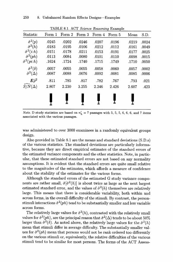
250 8. Unbalanced Random Effects Designs-Examples

TABLE 8.1. ACT Science Reasoning Example

Statistic Form 1 Form 2 Form 3 Form 4 Form 5 Mean S.D.

O'2(p) .0245 .0202 .0246 .0207 .0196 .0219 .0024O'2(h) .0183 .0195 .0106 .0212 .0112 .0161 .0049

O'2(i :h) .0151 .0178 .0211 .0153 .0191 .0177 .00250'2 (ph) .0113 .0084 .0080 .0101 .0110 .0098 .0015

O'2(pi :h) .1624 .1724 .1740 .1715 .1749 .1710 .0050

0'2 (J) .0057 .0055 .0055 .0058 .0060 .0057 .0002O'2(ß ) .0087 .0088 .0076 .0092 .0081 .0085 .0006

E ß2 .811 .785 .817 .782 .767 .793 .021-8jN(ß) 2.807 2.230 3.255 2.246 2.426 2.607 .423

I I , I , ,Note. D study statistics are based on n~ = 7 passages with 5, 5, 5, 6, 6, 6, and 7 iternsassociated with the various passages.

was administered to over 3000 examinees in a randomly equivalent groupsdesign .

Also provided in Table 8.1 are the means and standard deviations (S.D.s)of the various statistics. The standard deviations are particularly informa­tive, because they are direct empirical estimates of the standard errors ofthe estimated variance components and the other statistics. Note, in partic­ular , that these estimated standard erro rs are not based on any normalityassumptions. It is evident that the standard errors are quite small relativeto the magnitudes of the estimates, which affords a measure of confidenceabo ut the stability of the est imates for t he various forms.

Although the standard errors of the estimated G study var iance compo­nents are rather small, O'[O'2(h)] is about twice as large as the next largestesti mated standard error, and the values of O' 2 (h) themselves are relativelylarge. This means that there is considerable variability, both with in andacross forms, in the overall difficulty of the st imuli. By cont rast, t he person­st imuli interactions 0'2 (ph) tend to be substant ially smaller and less variableacross forms.

T he relatively large values for O'2(h), contrasted with the relatively smallvalues for O'2 (ph), are the principal reason that O'2 (ß ) tends to be abo ut 50%larger than 0'2(0). As noted above, the relat ively large values for the O'2(h)mean that stimuli differ in average difficulty. The substantially smaller val­ues for 0'2 (ph) mean that persons would not be rank ordered too differentlyon the various stimuli or , equivalent ly, the relative difficulties of the variousstimuli t end to be similar for most persons. The forms of th e ACT Assess-

8.2 District Means für ITED Vocabulary 251

ment undergo an elaborate equat ing process. This process is unlikely toadjust much for a2 (ph), but it eliminates (or , at least mitigates) constanteffects such as those captured by a2(h). Consequently, it is likely that thedifferences between a2 (D. ) and 172(8) have no particularly important con­sequences for the reported scores.

Contrary to some tenets of convent ional wisdom , reliabilities lower than.80 are not necessarily indicative of poor test s. Such results are to be ex­pected for relatively short tests that sample a heterogeneous conte nt do­main , as does the ACT Science Reasoning Test . (One of the exercises atthe end of this chapte r explores the sam ple sizes that might be used toobtain higher reliability with an increased time limit .) Note, also, that theabsolute-error SEM is V.0085 ~ .09, which is only abo ut a tenth of araw-score point , even with reliabili ties slight ly less th an .80.

In some testing programs, t he user of examinee data knows which formof the test was t aken by each examinee. Generally, this is not the casefor testing programs such as t he ACT Assessment , and usually t he exam­inees in any particular da ta set have t aken different forms . Consequently,"mean" st atistics such as t hose of Table 8.1 provide relevant answers toquest ions about erro r variances and coefficients. These mean results areact ually more st able than the standa rd deviations in the last column sug­gest. The standa rd deviations are estimated standard errors for a singleform. The est imate d standard errors for the "mean" stat ist ics are the st an­dard deviations divided by the square root of five.

It is evident that the means of the G study est imated variance compo­nents are quite st able, which makes them particularly useful in predicting Dstudy results for different sampie sizes and sarnple size patterns. Table 8.2provides est imated D st udy results for 40 and 35 items , for four differentnumbers of st imuli (4, 5, 6, and 7), and für two patterns of sample sizes.The first pattern consists of sample sizes that are about as equal as possi­ble, which gives a value of 11,~ that is quite elose to n~ . The second patternof sample sizes is more diverse, resulting in a smaller value of 11,,, . The firstline in Table 8.2 is a baseline; it provides results using the mean of t he Gstudy est imated vari ance components in Table 8.1 and the sample sizes forthe current ACT Science Test. It is evident from Table 8.2 that for fixedvalues of n~+ and n~, modest vari ation in sam ple size patterns does notmake much difference . However, decreases in n~+, and especially decreasesin n~ , cause not able increases in error var iances.

8.2 District Means for ITED Vocabulary

As an illustration of an unbalanced design in which a facet is nested withinthe obj ects of measurement , consider a G study (p :d) x i design für pupils(p) within school districts (d) in Iowa who took t he 40-item (i) ITED

252 8 . Unbalanced Random Effects Designs-Examples

TABLE 8.2. Different Sampie Size Patterns for ACT Science R eason ing Example

0'2 (8) 0'2 (ß) E p2 --I n ' n~:hv i S/N(ß)n i ± h n h

40 7 5,5,5,6,6,6,7 6.8966 .0057 .0085 .793 2.607

40 6 6,6,7,7,7,7 5.9702 .0059 .0091 .788 2.42140 6 5,6,7,7,7,8 5.8824 .0059 .0091 .787 2.40340 5 8,8,8,8,8 5.0000 .0062 .0099 .779 2.21540 5 6,7,8,9,10 4.8485 .0063 .0101 .777 2.17940 4 10,10,10,10 4.0000 .0067 .0112 .765 1.95840 4 8,10,10,12 3.9216 .0068 .0113 .764 1.936

35 7 5,5,5,5 ,5,5,5 7.0000 .0063 .0091 .777 2.41135 7 3,4,4,5,6,6,7 6.5508 .0064 .0093 .775 2.34635 6 5,6,6,6,6,6 5.9756 .0065 .0097 .771 2.25435 6 4,5,5,6,7,8 5.6977 .0066 .0099 .769 2.20635 5 7,7,7,7,7 5.0000 .0068 .0106 .762 2.07335 5 5,6,7,8,9 4.8039 .0069 .0108 .760 2.03335 4 8,9,9,9 3.9902 .0073 .0119 .749 1.84535 4 6,8,9,12 3.7692 .0075 .0123 .746 1.787

Note. The first line of results is based on th e means of the G study est imated variancecomponents in Table 8.1 using t he sampie sizes for the current ACT Science ReasoningTest .

Vocabulary Test (Form K, Level 17/18) (Feldt et al., 1994) administeredin the Fall of 1997. Table 8.3 provides the results of such a G study basedon a sampIe of about one-third of the pupils in approximately one-thirdof the distriets that took the ITED th at year . For illustrat ive purposes weassurne here that these data ean be viewed as a random effeets design,without taking into aeeount the eomplieating possibility of sampling froma finite popul ation of pupils and /or districts.!

The degree to which the design is unbalaneed is partly indicated by thegroup ed frequeney distribution of the np:d sample sizes at the bottom ofTable 8.3. At a finer level of det ail, the range of the 108 sample sizes was4 to 309, with a mean of 28.6 and a median of 17. The differenee betweenthe mean and the median is largely att ributable to several districts withquite large values for np:d.

Probably the most dramatic aspeet of the G study result s is the relativelylarge varianee eomponent for pupils, O'2 (p:d) ~ .034 eompared to the vari­anee eomponent for districts, O'2(d) ~ .002. Apparently, pupil variability(within districts) is about 17 times greater than district variability. This

1 Although the data are real , there are several aspects of thi s examp le that are ar­tificial. For exa mple, the analysis here is restricted to raw scores . Also, it is not toolikely that an act ua l investigati on would involve sampling one-t hird of t he districts andone-third of th e pupils wit hin each district.

8.2 Distr ict Means for ITED Vocabulary 253

TABLE 8.3. G Study Analysis ofa Sample of District Means for ITED Vocabulary

Effect df T SS MS 172

d 107 37013.57628 429.66310 4.01554 .00213p :d 2983 41666.42500 4652.84872 1.55979 .03412i 39 38417.57198 1833.65881 47.01689 .01509di 4173 39928 .01358 1080.77849 .25899 .00228pi :d 116337 67255.00000 22674 .13770 .19490 .19490

J.L 1 36583.91318

Number-Correct Metrie

np:d freq Mean Variance

4-10 20 19.6459 48.431811-20 43 21.6574 55.745821-40 37 20.9605 59.3581> 40 8 22.4115 66.4076

n p+ = 3091 and 2:d n;:d/n p+ = 81.62245

fact suggests that district -level coefficients may be smaller than pupil-levelcoefficients. This is not a cert ainty, however , because we do not yet knowhow large distriet error variances are relative to pupil error vari an ces. (SeeExercise 8.4.)

Using the same sample sizes as those in the G study, let us consider aD st udy (P :d) x I design , with districts as the objec ts of measurement.General results for t his design are treated in Secti on 7.2.3, with d hereplaying the role of c in Section 7.2.3. The harmonie mean of t he np:d is15.213. Using Equation 7.33, absolute error vari ance is

a2(L\) = .03412 .01509 .00228 .19490 = .003 .15.213 + 40 + 40 + 608.520 00

Recall from Section 7.2.3 that this result is not necessarily equal to theaverage of the 108 condit iona l absolute error variances (see Equation 7.35) .For these data , this average is .00266. In shor t , in terms of SEMs, a(L\) is.0548, while t he average a(L\d) is .0516. These esti mates are qui te simil ar ,given t he substantial lack of balan ce in t he data .

The vari an ce of t he unweighted distribution of distriet mean s is .00476,where each mean is expressed in the proportion-correct metrie. It followsthat an est imate d genera lizability coefficient for the G study sam ple sizesis

E - 2 = 172(d) = .00213 = .4471.

p S2(d) .00476(8.1)

254 8. Unbalanced Random Effects Designs-Examples

Alternatively, using Equation 7.37 relative error variance is estimated tobe

A2(8) = .03412 .00228 .19490 = 0(J 15.213 + 40 + 608.520 .0 262,

and an estimated generalizability coefficient is

.00213 _ 4 9------ .47 ..00213 + .00262

(8.2)

The estimates in Equations 8.1 and 8.2 are remarkably similar, given thesubstantiallack of balance in the data.

Recall that these D study results are based on one-third of the testedpupils in about one-third of the distriets. An investigator might weIl beinterested in the generalizability of the 108 distriet means when each meanis based on all tested examinees. The harmonie mean of these sample sizesis 45.640, whieh can be used in Equation 7.33 to obtain 0-2 (.6.) = .00129 andin Equation 7.37 to obtain 0-2 (8) = .00091. The latter leads to an estimatedgeneralizability coefficient of Eß2 = .7004, which is a "stepped-up" versionof the result in Equation 8.2 for the smaller sample sizes. We are not able toestimate a generalizability coefficient in the manner of Equation 8.1 becausewe have no direct estimate of observed score variance for the larger sam piesizes.

Strictly speaking, the results discussed in the previous paragraph arebased on only a sample of the districts. It is unlikely, however, that muchdifferent results would be obtained by using a larger sample of districts ,or even all the districts. Furthermore, as long as the number of distrietsis large enough to lead to an acceptably stable estimate of universe scorevariance, the magnitude of an estimated coefficient is not likely to be muchaffected by increasing the number of distriets.

If the G study were based on all th e districts in Iowa, and these districtswere viewed as the entire population of interest, there is an additional sta­tistical issue that merits consideration. In this case, it can be argued ratherconvincingly that districts are fixed, whieh suggests that the G study shoulduse a mixed-model analysis, not a random one. In most cases, with unbal­anced designs, the estimation of variance components for mixed modelsis an even more thorny subject than their estimation for random models.One approach that does not make distributional-form assumptions (e.g.,normality) is to use Henderson's (1953) Method 3. For the (p :d) x i de­sign, however, Henderson's Method 3 leads to the same decomposition ofthe total sums of squares as does Method 1 (the analogous-ANOVA pro­cedure). Consequently, equating sums of squares to their expected valuesleads to the same estimates of (J2(p:d), (J2(i) , a;?(di), and (J2(pi :d) for bothMethods 1 and 3. /

Under the mixed model , conventional statistieal terminology would notrefer to a variance component for distriets; rather, it would be called aquadratie form. Setting aside this terminologieal distinction, under the

8.2 District Means für ITED Vocabulary 255

mixed model, given the convent ions adopted in Section 3.5, fJ2 (d) that re­sults from equat ing sums of squares to their expected values, is an est imateof

Clearly, under the mixed model assumpt ions, fJ2(d) can be multiplied by(nd - l)/nd to obt ain a statistic with the conventional form of a variance.

This sidetrack into mixed models is something of a statistical technicalitythat has very little influence on est imates of error variances and coefficients.It is especially important to note th at the fixed part of the mixed modeldiscussed in this section is associated with the objects of measurement, notthe universe of generalizat ion. A fixed facet in the universe of generalizationis an ent irely different matter , as already discussed in Chapter 4, and asdiscussed more fully when we treat multivariate generalizability theory insubsequent chapte rs.

Given the complexit ies and ambiguit ies involved in est imat ing variancecomponents for unbalanced G study designs, it seems natural to considerthe possibility of randomly discarding data until a balanced design is ob­tained. Such an ad hoc procedure hardly deserves to be called a "design,"but it is a frequently employed strategy. Let us consider what might happenif a balanced design were employed for this ITED Vocabulary example.

The total number of pupils in the data set for the 108 districts is 309l.Obviously, if we want to obtain a balanced design, we would like to elimi­nate relatively few districts and pupils. For a particular number of pupils ,say n;, to obt ain a balanced design all distr icts with fewer than n; pupilsare eliminated; the dat a are retained for all distri cts with exact ly n; pupils ;and for districts with more th an n; pupils, a random sample of n; pupilsis drawn. So, for example, we could use all districts, but this would requireusing n; = 4, a very small value, that result s in including only 432 pupils(14%). If n; = 10, then the design will include 93 districts (86%) with atotal of 930 pupils (30%). If n; = 15, then the design will include a muchsmaller number of districts, 66 (61%), with a slightly larger total numberof pupils, 990 (32%). Let us consider using n; = 10.

Obviously, different est imated variance components will be obtained de­pending on which 10 pupils are sampled for districts having more than 10pup ils in the dat a set. This is illustrat ed by th e box-and-whiskers plots inFigure 8.1 based on 250 replicat ions of a balanced design with 10 pupilsper district . For each box, the lowest , middle, and highest lines are at the25th , 50th, and 75th percent ile points , respectively. The bottom whisker isat the 10th percentile point , and the top one at the 90th percentile point .The box-and-wh isker plots are ordered from left to right in terms of verticalaxis lengt hs. For d, di , i t he length is .0025; for p:d and pi :d the length isdoubled to .005. Therefore, if the first three plots were displayed using the

256 8. Unbalanced Random Effects Designs-Examples

0.0035

0.0030

0.0025

0.0020

0.0015

0.0010+----,

d

0.0040

0.0035

0.0030

0.0025

0.0020

0.0015+----,

di

0.0170

0.0165

0.0160

0.0155

0.0150

0.0145+-------,

0.034

0.033

0.032

0.031

0.030

0.029+-----,p:d

0.200

0.199

0.195+-------,

pi:d

FIGURE 8.1. Box-and-whisker plots of estimated variancecomponents for ITEDVocabulary based on a balanced design with 10 students per district and 250replications.

scale of the last two, the first three plots would be half as tall as they aredepicted in Figure 8.1.

It is important to note that the variability of the estimated variancecomponents in Figure 8.1 is not the result of true replications of a bal­anced design with 10 pupils per district. First, the districts and the itemsin each pseudoreplication are the same. Second, for each pseudoreplica­tion, the data are identical for those districts that have exactly 10 pupils.Third, the potentially variable data result from a stratified random sam­pling process that is conditional on the specific, fixed sizes for pupils in theoriginal data set. Although these three characteristics tend to make thepseudoreplications much more similar than they otherwise would be, thereis still evidence of variability for the estimates in Figure 8.1.

The dots in Figure 8.1 approximately locate the analogous-ANOVA esti­mates of the variance components using the original data. Except for a2 (d),these estimates are rather distant from the median of the pseudoreplica­tions estimates. Indeed, a2 (p:d) and a2(pi:d) are very different from thepseudoreplications estlmates.f Why? There are two cIasses of reasons: thecharacteristics of the eliminated data and differences in estimation proce­dures .

The pseudoreplications in Figure 8.1 are based on eliminating all dis­tricts with fewer than 10 pupils. Clearly this may distort estimates if theeliminated districts are unlike the retained ones. The bottom part of Ta­ble 8.3 provides relevant information. For example, there were 20 districtswith sample sizes of 4 to 10 pupils per district. The unweighted average,over these 20 districts, of the mean number-correct score for each district

2The absolute magnitudes of the differences might not be judged very large, but therelative magnitudes are considerable.

8.3 Clinical Clerkship Performance 257

was 19.6459 items correct . Similarly, the average of the observed varianceswas 48.4318. It is apparent from Table 8.3 that the observed means andvariances tend to increase with increases in np:d ' This clearly suggests thatdistricts with 10 students are not interchangeable with districts with largernumbers of students, which will cause discrepancies between the estimatesfor the unbalanced and balanced designs.

The positive relationship between np:d and the sampie statistics willcause other differences, too. For example , the few large districts, whichhave the largest means and variances, will have less of an influence onestimated variance components for the balanced data set .

The above arguments should not be construed as meaning that the full­data estimates in Table 8.3 are necessarily "bettet" than estimates basedon a balanced design with, say, 10 students per district . We may arguethat the full-data estimates are more stable because they are based onlarger sampie sizes, but that does not necessarily mean that the full-dataestimates are closer to the parameters. The essence of the problem is that wehave differences not only in sampie sizes but also in estimation procedures.We know a great deal about the characteristics of the estimates for thebalanced design with the smaller sample sizes, but very little about theanalogous-ANOVA estimates for the full data set.

Still, "squaring off" an unbalanced data set by randomly eliminatingdata has two problematic characteristics: it frequently results in discardinga large amount of data, and the process used to eliminate data is conditionalon sampie sizes in the data set and can lead easily to eliminating data thatare not representative of the full data set . For these reasons, this authoris not sanguine about the procedure, except when only a small amount ofdata needs to be eliminated and there is strong reason to believe that theeliminatcd data are representative.

8.3 Clinical Clerkship Performance

Kreiter et al. (1998) discuss certain psychometrie characteristics of a stan­dardized clinical evaluation form (CEF) used to evaluate the performanceof medical students in various clinical clerkships at a large midwestern med­ieal school. The CEF consists of 19 items measuring behaviorally specificskills judged to be important in clinical performance (e.g. "Accepts respon­sibility for actions") . Ratings are based on a five-point scale ranging from"unacceptable" to "outstanding." Standardized CEFs are often the onlyformal feedback that students receive about their clinical performance inthe clerkships . As such, th e information provided by the CEFs serves animportant role in student assessment , including grading.

Typically, each student is observed by a small number of raters demon­strating his or her clinical skills in real-time and real-world settings. So,

258 8. Unbalanced Random Effects Designs-Examples

TABLE 8.4. G Study for Surgery from Kreit er et al. (1998)

Effect df T SS MS 0-2

P 174 303099.82461 1993.57134 11.45731 .07066r: p 730 306388.57895 3288.75434 4.50514 .22713i 18 301484.60221 378.34894 21.01939 .02300pi 3132 304111.86118 633.68763 .20233 .00245ri :p 13140 309893.00000 2492.38448 .18968 .18968J.L 1 301106.25327

n r :p freq mean n r :p freq mean

2 6 4.2675 7 16 4.16123 24 4.3187 8 4 4.39144 19 4.1025 9 4 4.42405 56 4.1752 10 1 3.46326 44 4.1583 11 1 1.0096

n r+ = 905 and I: n;:p/nr+ = 5.64972

while the instrument is standardized, many other condit ions of measure­ment are not . The Kreiter et al. (1998) study was designed to examine :(i) the magnitudes of the variance components associated with the CEFand the population; (ii) the effect on measurement precision of varying thenumb ers of raters and items ; and (iii) the minimum number of CEF obser­vat ions required to obt ain a reasonably precise measure of performance fora student . Here, these issues are summarized for surgery only, which is oneof six clerkships that students typically experience in a clinical year.

Medical faculty, residents, and adjunct faculty who worked with studentsduring the surgery clerkship filled out a CEF for each student. As is of­ten the case in real-world settings, there was no fully formalized designthat assigned specific raters, or a specific number of raters, to each stu­dent. A total of 175 students was evaluated by 76 raters, with a mean of7.1 ratings per student. No rater evaluated all students, but most ratersevaluated a number of st udents. Clearly, raters are not crossed with stu­dents, but neither are they complete ly nested within students . Kreiter etal. (1998) treat the data as a G study for the (r :p) x i design. This choiceis partly one of convenience, but it does not seem too unreasonable underthe circumst ances. (Some consequences of this choice are considered in Ex­ercise 8.7.) The (r :p) x i design is formally identical to both the p x (i: h)and the (p :c) x i designs; so the results in Section 7.1.3 and Appendix E,respectively, apply with obvious changes in notation.

8.3 Clinical Clerkship Performance 259

0.6 0.8

111 1 I I I 11 11 11111111110.7 8 8 8 88 8 8 8 8 8 88 8 8 8 8 8 8 88 8

0.5 'E:E s 0.6 555555555555555555555~ 0.4 ==

222222222222222222222~ 0.5e o 3 3 3 3 3 3 3 3 3 3 3 3 3 3 3 3 3 3 3 3 3

~0.3 3333333333333333 3 3 333 ~0.42222222222 222 22222222(]) :i5:;

5555555555555 55555555 '"(5 ~0.31l0.2 8 88 8888 88888888888888 e!« (]) 1111111 111111111111115i 0.2

0.1 Cl0.1

0.0 ,. .o 5

j i i i i I i i i i I i

10 15 20Number of Items

I I25

0.0 ,. .o 5

, I ' i i i I i' 'i10 15 20

Number of Items

'i25

FIGURE 8.2. Estimated absolute error SEMs and generalizability coefficientsfor surgery from Kreiter et al. (1998) with n~ = 1, 2, 3, 5, and 8 raters and5 ::; n; ::; 25 iterns.

Table 8.4 on the preceding page provides random-model G study resultsfor the Kreiter et al. (1998) surgery data. The distribution of number ofratings is provided at the bottom of the table, which is one way of char­acterizing the extent to which th e data are unbalanced. The number ofratings ranged from 2 to 11, but over 80% of the students were evaluatedby 3 to 6 raters. The largest est imated variance component is for raters,which is not unexpected given the variabilities of their backgrounds, theirsometimes limited familiarity with the students , and the nonstandardizedcircumstances of their rat ings.

Since 8'2(r :p) is so large, it seems unlikely that a single rating wouldlead to acceptably reliable scores for students. This intuitive judgment andother result s are formalized in Figur e 8.2, which provides random-modelabsolute error SEMs, 8'(~) , and est imated generalizability coefficients for5 to 25 items and 1, 2, 3, 5, and 8 raters." Kreiter et al. (1998) concludedfrom a slightly different presentation of these results th at three or moreraters provide an acceptably reliable measure of student performance usingthe full-length CEF. They also suggested that , from the perspective ofmeasurement precision, the CEF could be shortened. (Other substantivevalidity concerns might not support doing so).

It is important to note that the estimat ion of the G study variance com­ponents was based on an unbalanced design, not because that is the optimalway to collect dat a, but rather because th at is the manner in which the

3rt is ass umed here th at items are random. If the only items of interest were those 19it ems in t he CEF , as spec ified, then it might be argued t hat items should be treated asfixed . T his aut hor seldom t reats ite ms as fixed , however , becaus e almost a lways sp ecificitems are representati ve of some larger set .

260 8. Unbalanced Random Effects Designs-Examples

dat a arose. In this sense, the lack of balance did not arise by "design." Onthe other hand, the D study considerations in the previous paragraph wereaddressed using a balanced design, because the principal questions involverecommended use of the CEF, and the psychometrie consequences of suchuse.

There is no logie in the results presented here to suggest that the D st udydesign should be unbalan ced. Of course, in practice, operational use of theinst rument might result in an unbalanced design. If so, an estimated condi­tional SEM, &(ß p ) , could be obt ained for each student based on the actualnumber of ratings for that student . Also, th e equations in Section 7.2.3,with obvious changes in not ation, could be used to est imate overall ab­solute error variance, generalizability coefficients, and other parameters.For example, suppose the operational use of the CEF generally required aminimum of three ratings per student, but more could be used, and tworatings would be accepted in unusual circumstances. What would be theest imated absolute-error SEM for 200 students if 15% had two ratings, 75%had three ratings, and 10% had four ratings? Under these circumst ances,the harmonie mean is nr = 2.85714, and using Equation 7.33 we obtain&(ß) ~ .29.

As we did in the previous sect ion, let us now consider what est imatedvariance components might have result ed from a balanced design created byrandomly discarding data. The lower part of Table 8.4 provides frequenciesand means for the numbers of ratings (2 to 11) made for the 175 st udents .The total number of ratings is n r+ = 905. Ifwe want to eliminate ratings tocreate a balanced design, a little computat ion leads to the conclusion thatthe fewest rat ings are eliminated using a balanced design with five raters.Under these circumstances, all students with fewer th an five ratings areeliminated; the ratings are retained for students with exactly five ratin gs;and for students having more than five ratin gs, a random sample of fiverat ings is used. This results in retaining 126 students (72%) and 630 ratin gs(about 70%).

Obviously, different estimated variance components will be obt ained de­pending on whieh five scores are sampled for students having more thanfive ratings. This is illustrated by the box-and whiskers plots in Figure 8.3based on 250 replications of a balanced design with five ratings per student.The plots are ordered from left to right in te rms of vertical axis lengths.For p, r:p , and ri:p the length is .02; for i and pi the length is five timessmaller . Therefore, if the last two plots were displayed using the scale ofthe first three, the last two plots would be five tim es shorter th an they aredepieted in Figure 8.3.

These are pseudoreplications, not true ones. The students and the itemsin each pseudoreplication are the same, and the sampling process is condi­t ional on the specific fixed sample sizes (6, 7, ... , 11) in the original dataset . Although the pseudoreplications are much more similar th an t rue ones,

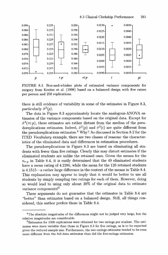
8.3 Clinical Clerks hip Performance 261

0.090 0.235 0.200 0.0230 0.0050

0.088 0.233 0.198 0.0225 0.00450.086 0.231 0.196

0.0220 0.00400.084 0.229 0.194

0.082 0.227 0.192

$0.0215 0.0035

0.080 0.225 0.190 0.0210 0.0030

0.078 0.223 0.188 0.0205 0.00250.076 0.221 0.186

0.0200 0.00200.074 0.219 0.184

0.072 0.217 0.182 0.0195 0.0015

0.070 0.215 0.180 0.0190 0.0010

P rtp ritp pi

FIGDRE 8. 3. Box-and-whisker plots of estimated variance com po ne nts forsurgery from Kreiter et al. (1998) based on a ba lanced design with five ratersp er p erson and 250 replications.

there is st ill evidence of variability in some of the est imat es in Figure 8.3,part icularly (; 2(p).

The dots in Figure 8.3 approximately locat e the analogous-ANOVA es­timates of t he variance components based on t he original data. Except for(;2 ( ri:p), these est imates are rather distant from the median of t he pseu­doreplications est imates . Indeed , (;2(p) and (;2(i) are quite different fromthe pseudoreplications est imates ." Why? As discussed in Section 8.2 for theIT ED Vocabulary example, there are two classes of reasons: the characte r­ist ics of the eliminate d dat a and differences in est imat ion procedures.

The pseudoreplications in Figure 8.3 are based on eliminat ing an st u­dents with fewer than five ratings. Clearly this may distort est imates if theeliminated st udents are unlike t he ret ained ones. Given the means for t hen r :p in Table 8.4, it is easily determined th at the 49 eliminated st udentshave a mean rat ing of 4.2286, while t he mean for the 126 retained st udentsis 4.1515-a rather large difference in t he context of t he means in Table 8.4.This explanation may appea r to imply that it would be better to use anstudents by simply sampling two ratings for each of them. However , doingso would lead to using only about 39% of the original data to est imatevariance components l''

These arguments do not guarantee that the est imates in Table 8.4 are"bette r" t han esti mates based on a balanced design. Still , an things con­sidered, t his aut hor prefers t hose in Table 8.4.

4The abso lute magnitu des of the differences might not be judged very large, but therelat ive magnitudes are considerable.

5Estimates for 1000 replicatio ns were obtained for two ratings per st udent . T he esti ­mat es were more var iable than those in Figure 8.3 for five rat ings, as is to be expec tedgiven the reduced sampie size. Furthermo re. the two-ratin gs esti mates te nded to be evenmore different from the full-data estimates tha n did the five-ratings est imates .

262 8. Unbalanced Random Effects Designs-Examples

8.4 Testlets

Testlets, as the name implies, have been defined as smaIl part-tests in alarger test (Wainer & Kiely, 1987; Wainer & Lewis, 1990; Sireci et al. , 1991).Lee et al. (2001) have defined a testlet as a subset of one or more items ina test form, which is treated as a measurement unit in test construction,administration, and/or scoring. This definition differs from others that havebeen proposed in two important ways: it refers explicitly to test forms,and the definition permits single-item testlets. In effect, the ACT ScienceReasoning example in Section 8.1 is an analysis of a test composed oftestlets.

The discussion of testlets here involves consideration of both balancedand unbalanced random effects designs, as weIl as a mixed model thatforeshadows a multivariate design. As such, this section can be viewed asthe beginning of a transition to multivariate generalizability theory.

There are a number of analytic procedures that have been proposed andused to analyze testlets, most of them based on an IRT model of one kind oranother. Here, we consider testlets from the perspective of generalizabilitytheory. In particular, we concentrate on sample size issues, aggregationissues, and fixed-versus-random issues.

In considering testlets, it is important to distinguish between a test anda form of a test. A test is a generic characterization of the multiple formsthat might be created using the test specifications. So, for example, "ACTScience Reasoning" is an identifier of a test, but there are many extantforms of this test, and many other forms that could be created. (Even ifonly one form of a test is available, the concept of a form is still relevant,because other forms could be created from the same specifications.)

Four Designs

Let us reconsider the synthetic data in Table 7.5 for a test form composedof eight items that are distributed across three testlets. We consider fouranalyses of these data, with the discussion framed in terms of reliabilityconsiderations. For the moment, we are not arguing which of these analysesis preferable; we are simply examining the assumpt ions and consequencesof these analyses .

1. D Study p x H Design. Suppose this test is conceptualized as be­ing composed of three random testlets, with the scores for the threetestlets used as the sole basis for analysis . In this case, the D studydesign is p x H, with nh = 3, but there are still two possible anal­yses. It is easily verified that, if total scores for the three testletsare employed, then E{J2 = .598; if unweighted mean scores are used,E{J2 = .684.

8.4 Testlets 263

2. D Study p x (I :H ) Random EjJects Design. Section 7.2.2 providesresul ts for t he unbalanced p x (I: H ) random effects design . In par­tic ular , Eq uat ion 7.32 gives E ß2 = .716.

3. D Study p x 1 Design. If the testlets are ignored , with t he indiv idua lit ems t reated as an undifferenti at ed set, t hen E ß2 = .885.

4. D Study p x (1 :H ) Design with H Fixed. The testlets could be viewedas fixed . Since t he design is unbalanced , t his possibility is not easilyaccommodated in univariate genera lizability t heory. A full discus­sion awaits our consideration of multivari ate generalizability theoryin Chapters 9 and 10. Here, we simply note that stratified alpha(Cronbach et al., 1965) is an appropriate generalizability coefficient,and it is .941 for these data.

Since the esti mated generalizability coefficients for these four designs arebased on a very small set of highly synt het ic data, no particular conclu­sions should be drawn based on t he absolute magnitude of t he estimates.However , t he relative magnitudes of t he coefficients (1 = lowest ; 4 = high­est) are largely predict able from by underst anding what is fixed and whatis random in t he various designs, what effects are confounded in certaindesigns , and how sarnple sizes affect the coefficients.

The analyses using the p x H design are t he simplest in the sense t hatthey require t he least amount of computation, but t hey involve concep­t ual complexities and amb iguities. One potential amb iguity is t hat E ß2 isdifferent for the total and mean score metrics, because different numbersof items are summed or averaged for t he t hree testlets. Ot her complexi­t ies arise because t he role of items is hidden in t he design, which leads toconfou nded effects. For cxample, a-2 (pH ) from t he p x H design representsthe confounding a-2 (pH ) and a-2 (pI :H ) from t he p x (I :H ) random effectsdesign.

T he p x I ana lysis is comp utationally simple but, for t he dat a in Ta­ble 7.5, t he ana lysis is also conceptually simplist ic, because it assumes t hatt he eight items represent a single random facet. T his design effectively as­sumes that a different form of t he test would include a different set of eightundifferenti ated items, without any considerat ion of their role in testl et s.The higher value of the est imated genera lizability coefficient for the p x 1design , compared to t he p x H design, is attributable largely to the factthat the average covariance for t he eight item scores (1.30) is larger thanthe average covariance for t he three testlet mean scores (.98) .

For the p x (I :H) random effects design , both items and testl ets aret reated exp licit ly as random, with a recognition t hat t here are differentnumbers of it ems associated with tes tle ts. This means t hat a different formof t he test would involve different items and different testlets, but t he sam­ple size patterns would be th e sam e. The analysis may be somewhat com­plex , but there are no particular concept ual ambiguities, and the analysis

264 8. Unbalanced Random Effects Designs-Examples

faithfull y reflects the structure of th e test form. Since items and testletsare random, variability in both facets cont ributes to error, and the analysisreflects this explicit ly.

Cases 2 and 4 have the same design st ruct ure, P x (I :H ); that is, theyboth bundle the items in the same manner. However, in Case 2, the testletsare a random facet , whereas they are fixed in Case 4. Case 4 would be appli­cable, for example, if items were associated with three content categories,all of which would be involved in every form of a test . Since H is fixed,variability in scores attributable to content categories does not affect errorvariance. Consequently, a generalizability coefficient for this design withH fixed will be larger than when H is random . The univariat e p x (I :H )design with H fixed can be viewed from the perspective of multivariategeneralizability theory in which the content categories are the multiple de­pendent variables, and there is a p x 1 design associated with each category,as discussed more fully later in Section 9.1. This multivariate perspectiveovercomes the unbalanced-design problems of a univariate mixed model.

It may not be clear why the p x (1:H) design with H fixed leads toa larger estimated generalizability coefficient than for the p x 1 design.After all, both involve the same number of items, and both view items asrandom. The reason for the difference is that the variance attributable tothe inter act ion of persons and testlets is effectively part of error variancefor the p x 1 design, whereas it is part of universe score variance for t hep x (1: H) design with H fixed.

In considering these four testlet analyses of the same data, it is naturalto ask which one is best. There is no unequivocal answer to th is quest ionwithout an unam biguous specification of t he universe of generalizatio n in­cluding, in particular , the identification of which facets are fixed and whichare random. However , both the p x H and p x 1 analyses have the distinctdisadvantage of hiding a facet.

Single-Item Testlets

Suppose the test specifications require that each form of a geomet ry testcontain an item that tests the Pythagorean theorem. From the perspec­tive of the content categories in a table of specifications, the PythagoreanTheorem item in a particular form represents a fixed condit ion of measure­ment. However, the particular Pythagorean Theorem items in the variousforms of the test will be different. From this perspective, the PythagoreanTheorem items const itute a random facet . In asense, then, when we focuson a single form of the test , the single Pythagorean Theorem item can beviewed as having both fixed and random features. Any particular analysisof the single-form data, however , will necessarily t reat the item as eitherfixed or random.

For example, if such an item is included in a test form that is analyzed us­ing t he p x 1 design, then t he item will be t reated as random. By cont rast ,

8.5 Exercises 265

in IRT , items are effect ively fixed, or to be more specific, the item param­eters are fixed, and a replication would involve identically the same itemparameters, resulting in strictly parallel forms. This difference in underlyingassumptions has a number of consequences that are rarely recognized. Forexample, estimated SEMs under the two models have different statisticalcharacterist ics (see, e.g., Lee et al., 2000).

It is important to underst and th at the fixed and random features of oursingle Pythagorean item are totally confounded in examinee responses. Todisconfound these features, at a minimum we need data for at least twoPythagorean items t aken by the same examinees. Then we can determinehow much variability in examinee responses to all of the items in a testform is attributable to the Pythagorean Theorem fixed category, and howmuch variability is at t ributable to different items that test the PythagoreanTheorem. Knowing this , we may then est imate D study results when a formincludes a single-item Pythagorean Th eorem testlet.

As a simple example in a somewhat different context , consider a writ­ing assessment in which each form contains one narrative prompt and oneinformative prompt, and suppose we are willing to assume that varianceat t ributable to rate rs is negligible. Presumably, the universe of generaliza­t ion has I :H , with H (genre) fixed and I (items-within-genre) random .To disconfound th e fixed/ random aspect of the genre/prompt dist inct ion,suppose we conduct a G study using the p x (i :h) design in which there aretwo prompts for each genre. Then, using the balanced-design mixed modelD study results in Chapter 4, the genre effects are distinguishable from theprompt effects, and an est imated generalizability coefficient for a test formwith one prompt for each genre is

Of course, in many realistic contexts that involve single-ite m testlets ,the designs are unbalanced. For example, a 20-item test form based onspecificat ions for five fixed content categories might consist of 5 items fromone category, 6 from another, 7 from a third, and 2 single-item testlets.For such complex cases, procedures in multivariate generalizability theorycould be employed.

8.5 Exercises

8.1* Form 1 of the ACT Assessment Science Reasoning Test in Table 8.1was administered to 3458 examinees. The resulting analogous T termswere:

266 8. Unbalanced Random Effects Designs-Examples

T(p) = 61977.95000T(i:h) = 62005.88433

T(pi:h) = 89416.00000

T(h) = 60279.46591T(ph) = 69160.59524

T(f.L) = 57802.35003.

Verify the results reported in Table 8.1 for Form 1.

8.2* Using only the "mean" results in Table 8.1 for the ACT ScienceReasoning Test, what is an estimated value of E p2 for the p x Idesign? Why is this a questionable estimate of reliability for thistest?

8.3* For the ACT Science Reasoning Test discussed in Section 8.1, assurnethat each passage takes two minutes to read , and each item requiresan additional half-minute to answer. Under these assumptions, whatsample sizes (nh and n~+) and sarnple size patterns (the n~:h) wouldgive E p2 ~ .85 with testing time no longer than 50 minutes? Use the"mean" results in Table 8.1 to answer this question. Of these alterna­tives , which is likely the most acceptable from a practical perspective?Why?

8.4 For the ITED Vocabulary example in Section 8.2, assuming G andD study sam ple sizes are the same, what is the signal-noise ratio fordistrict means , using absolute error variance as noise? What is thissignal-noise ratio for pupils in a randomly selected district? What isthis signal-noise ratio for pupils across all districts?

8.5 For the medical clerkship example in Section 8.3, suppose that thegrade for a student is the rounded average of three ratings based onusing the current 19-item CEF. Under the assumption that errorsare normally distributed, what is the probability that students witha universe score of 4 will receive a grade of 3 or lower?

8.6 For the circumstances and assumptions in Exercise 8.5, what is theprobability that two examinees with the same universe score will beassigned different grades? For two examinees, p and q, assurne thisquestion is asking for Pr (IXp - X qI>.5 I f.Lp = f.Lq ), where X p andX q are the unrounded average ratings.

8.7* In discussing the medical clerkship example in Section 8.3, it wasnoted that, in the actual data set, raters were neither fully nested norfully crossed. The analysis, however, was conducted as if the ratingswere fully nested. Discuss the G study and D study consequencesof this decision , under the assumption that there is no systematicassignment of raters to students. In particular, consider what o-(~)

and E p2 might be if the D study design had raters crossed withstudents.

8.8* Verify the numerical results reported in Section 8.4 for testlets.

9Multivariate G Studies

It too k Cronbach and his colleagues nearly 10 years to write t heir 1972monograph . This rather long tim e period is directly related to their effortsin developing multivariat e generalizability t heory, which they regard as theprin cipal novel cont ribut ion of their work. In mult ivariat e generalizabilityt heory, each object of measurement has multiple universe scores, each ofwhich is associated with a condit ion of one or more fixed facets, and thereis a random-effects variance components design associated with each fixedcondit ion. These rand om-effects designs are statistically "linked" throughcovariance components to yield a multivariate design.

Obviously, a univariat e random model is a special case of a multivari­ate model. Also, a univariate mixed model is merely a simplification of amultivariat e model. It follows that generalizability theory is essent ially arand om effects theory, and univariat e generalizability theory is best viewedas a special case of mult ivariat e generalizability theory.

Cronbach et al. (1972, Chaps. 9 and 10) provide an exte nsive treat­ment of multivariate generalizability theory. Int roduct ions are provided byBrennan (1992a) , Shavelson and Webb (1981), Shavelson et al. (1989), andWebb et al. (1983). The treatment of multivariat e generalizability theoryin t his book is heavily influenced by Cronbach et al., but there are notabledifferences in emphas is, notation, and scope.

Multivariate generalizability t heory is ext raordinarily powerful and flex­ible. However , t his power and flexibility are purchased at t he price of chal­lenging conceptua l and statistical issues. Many of t he conceptual challengesare associated largely with characte rizing multivar iate designs and uni­verses. Most of t he statistical challenges focus on t he est imat ion of covari-

268 9. Multivariate G Studies

ance components. For these reasons, this chapter is dominated by a detaileddiscussion of multivariate G study designs and procedures for estimatingG study covariance components.

This chapter's treatment of G study design structures includes both bal­anced and unbalanced situations, but procedures for estimating covariancecomponents are restricted to balanced designs. Estimation procedures forunbalanced designs are considered in detail in Chapter 11.

We begin with abrief overview of multivariate generalizability theoryprimarily using the so-called "table of specifications" model as an example .In this example, we consider G study issues and a subset of the D studyissues that might be addressed. The remainder of the chapter is devoted toG study issues only.

9.1 Introduction

In the mid 1960s Cronbach, Gleser, and Rajaratnam published aseries ofthree papers in which they outlined the basics of generalizability theory.Each of them was the first author for one paper. Two papers (Cronbach etal., 1963; and Gleser et al., 1965) focus on univariate generalizability, whilethe third (Rajaratnam et al., 1965) provides a simple but elegant snapshotof their early thinking about multivariate generalizability theory. In asense,this third paper is a generalizability theory perspective on what is nowoften called stratified alpha, which was also considered from a classicalperspective by Cronbach et al. (1965) at about the same time. In the early1980s, Jarjoura and Brennan (1982, 1983) extended the basic model inthe Rajaratnam et al. (1965) paper. They referred to it as the "table ofspecifications" model.

In this model, there is a different set of items nested within each ofthe levels of a fixed facet, such as the content categories in a table ofspecifications . To say the content categories are fixed is to say that everyform of the test would involve the same categories of items. The itemsthemselves are random in the sense that each form of the test would involvea different set of items for each category. For different categories of items ,v and v', the model equations would be

(9.1)

and

(9.2)

9.1 Introduction 269

where v and ~ designate effects for v and v', respectively.' That is, there isa random effects p X i design associated with each level of the fixed facet .The fixed levels are linked in the sense th at th e same persons respond toall items in both levels. Note that t he items in v and v' are not the same;nor is it required that the G study number of items be the same for v andv' . We designat e this multivariat e design as p. x i", with the number oflevels of the fixed facet being nv .

The parameters under eonsiderat ion are variance and covariance com­ponents for the population and universe of admissible observat ions, whiehcan be grouped into th e following three symmetrie matrices.

~p [ O"~(p) O"vv' (p) ] (9.3)O"vv' (p) O"~, (p)

~i [ O"~ (i) ] (9.4)O"~, (i)

~pi [ O"~(pi) ] (9.5)O"~ , (pi)

The diagonal elements are th e variance eomponent s for v and v'. The co­vari ance between universe scores in the off-diagonal positions of ~p is

(9.6)

The ~i and ~pi matrices are diagonal because each level of v has a differentset of items associated with it . T he fact that th ese matrices are representedusing only two rows and two eolumns does not mean th at there are neces­sarily only two levels of the fixed facet . This compaet form simply indicatesthe notation used to represent the elements of t he n v x n v matrices.

As an example, consider th e synthetic data in Table 9.1 where n v = 3.This is the same data set used by Rajaratnam et al. (1965) to illustrat e whatth ey called the "genera lizability of stratified-parallel test s." Also, thesedata were used in Seetion 8.4 to illustrate considerat ions about testlets.The bottom part of Table 9.1 provides the mean squares and est imatedvariance components for each of the th ree levels of v .2 For any pair oflevels of v , the observed covarianee is

(9.7)

1Readers should be careful not to confuse the lowercase Roman letter v wit h thelowercase Gr eek letter u, Note, also, that in t he Cronbach et al. (1972) not ational system,v and V i would be used as prescr ipts.

2Somet imes v refers to t he enti re set of fixed cond itions, and sometimes it refers to asp ecific conditio n. This notationa l Iiber ty simplifies notational conventions. T he contextmakes it clea r how v is to be interpret ed .

270 9. Multivariate G Studies

TABLE 9.1. Synthetic Dat a Example for p. x iODesign

Vi V2 V3

P i i i2 i i i2 i3 i4 i i i2 X pi X p2 X p3 X piXp2 X piXp3 X p2Xp3

1 4 5 3 3 5 4 5 7 4.50 3.75 6.00 16.8750 27.0000 22.50002 2 1 2 3 1 4 4 6 1.50 2.50 5.00 3.7500 7.5000 12.50003 2 4 4 7 6 5 8 7 3.00 5.50 7.50 16.5000 22.5000 41.25004 1 3 5 4 5 5 4 5 2.00 4.75 4.50 9.5000 9.0000 21.37505 3 3 6 7 5 7 8 9 3.00 6.25 8.50 18.7500 25.5000 53.12506 1 2 5 6 4 4 5 6 1.50 4.75 5.50 7.1250 8.2500 26.12507 3 5 6 8 6 7 7 8 4.00 6.75 7.50 27.0000 30.0000 50.62508 0 1 1 2 0 4 7 8 0.50 1.75 7.50 .8750 3.7500 13.1250

Mn 2 3 4 5 4 5 6 7 2.50 4.50 6.50 12.5469 16.6875 30.0781

Vi V2 V3

MS(p) 3.7143 12.2143 4.1423S12(p) = 1.4821MS(i) 4.0000 2.6667 4.0000

MS(pi) .5714 1.0714 .4286 S13(p) = .5000S23(P) = .9464

a2(p) 1.5714 2.7857 1.85718"2 (i) .4286 .1994 .4464

8"2 (pi) .5714 1.0714 .4286

which is an unbiased est imator of the covariance between universe scores.That is, for the p. x iO design,

(9.8)

These est imated variance and covariance components can be displayedin the following three matrices.

[ 1.5714 1.4821 .5000 ]~p = 1.4821 2.7857 .9464

.5000 .9464 1.8571

[ .4286

.4464 ]f:i = .1994

[.5714

.4286 ] .~pi 1.0714

Suppose the universe of generalization consists of randomly parallel testswith two, four, and two items for Vi, V2, and V3, respectively. This meansthat the G study and D study sample sizes are the same, and the est imated

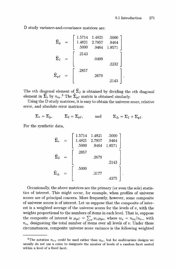
9.1 Introduction 271

D study variance-and-covariance matrices are:

[1.5714 1.4821 .5000 ]:Ep 1.4821 2.7857 .9464

.5000 .9464 1.8571

[.2143

.2232 ]:EI .0499

[.2857

.2143 ] .:EpI = .2679

The vth diagon al element of ~I is obtained by dividing t he vth diagonaleleme nt in ~i by n iv .3 T he ~pI matrix is obtain ed similarly.

Us ing t he D study matrices, it is easy to obtain the un iverse score, relativeerror, and abso lute error matrices:

:Er = :Ep , :Eo = :EpI , and :EL\ = :EI + :EpI .

For the synthetic dat a ,

[1.5714 1.4821 .5000 ]

:Er 1.482 1 2.7857 .9464.5000 .9464 1.8571

[ .2857

.2143 ]:Eo = .2679

[.5000

.4375 ] .:EL\ .3177

Occasionally, t he above matrices are t he primar y (or even t he sole) statis­tics of interest . T his mig ht occur, for example, wh en profiles of universesco res are of principal conce rn. More frequently, however , some compositeof universe scores is of interest . Let us suppose t hat t he composite of inter­est is a weighted average of t he universe scores for the levels of v, with t heweights propor tional to t he numbers of items in each level. T hat is, sup poset he composite of interest is J.Lpc = L:v wv J.Lpv, where W v = niv/ni+, wit hn i+ design at ing t he total number of items over all levels of v . Under t hesecircumstances, composite universe score variance is t he following weig hted

3The notation n i :v could be used rather than niv. but for rnultivariate designs weusually do not use a colon to designate the nurnber of levels of a randorn facet nestedwithin a level of a fixed facet.

272 9. Multivariate G Studies

sum of all of the elements in :Ep :

aß(p) = l: w~a~(p) +l:l:wvwv,avv'(p) .v v#v'

For the synthetic data, the W v weights are .25, .50, and .25, and

(9.9)

aß(p) (.25)2(1.5714) + (.50)2(2.7857) + (.25)2(1.8571)

+ 2(.25)(.50)(1.4821) + 2(.25)(.25)( .5000) + 2(.50)(.25)(.9464)

= 1.5804.

Assuming the estimator of composite universe score is Xpe = ~v wvXpv,relative error variance for the composite is the following weighted sum ofthe diagonal elements of :Eo,

(9.10)

and absolute error variance for the composite is the following weighted sumof the diagonal elements of :Et>,

(9.11)

For the synthetic data in Table 9.1,

aß(J) = (.25)2(.2857) + (.50)2( .2679) + (.25)2(.2143) = .0982

and

aß(ß) = (.25)2(.5000) + (.50)2(.3177) + (.25)2( .4375) = .1380.

A multivariate generalizability coefficient can be defined as the ratioof composite universe score variance to itself plus composite relative errorvariance. Similarly, a multivariate phi coefficient can be defined as the ratioof composite universe score variance to itself plus composite absolute errorvariance. For the synthetic data example considered here, the estimates ofthese coefficients are Eß2 = .941 and (j; = .920. With the w weights beingproportional to the sample sizes, Eß2 is stratified 0: .

The example that has been considered in this section involves unequalnumbers of conditions nested within each of the levels of a fixed facet. Froma univariate perspective, this would require a mixed-model analysis of anunbalanced p x (i :v) design. Using such an analysis to estimate variancecomponents would be quite complicated, whereas the multivariate analysisis rather straightforward.

When there are an equal number of conditions within each level of thefixed facet, the univariate analysis is rather simple (see, e.g., Sections 4.4.2

9.2 G Study Designs 273

and 5.1.3), and the ANOVA variance component estimates for the univari­ate analysis (J"2(alV) are easily expressed in terms of ANOVA variance andcovariance component estimates for a multivariate analysis. In particular,a2(plV) is the average of the elements in ~p ; that is,

(9.12)

where avv'(p) = a~(p) when v = v'. Also, a2(pvlV) is the difference be­tween the average of the variance components in ~p and the average of thecovariance components; that is,

(9.13)

Finally, a;(i:vlVl.. and a2(pi :vlV) are the averages of the variance compo­nents in ~i and ~pi, respectively :

a2( i:vlV) L a~(i) (9.14)

v nv

a2(pi:vlV) L a~(pi). (9.15)v nv

These equalities illustrate that variance components from a univariate bal­anced design can be viewed as simple averages over the conditions of afixed facet . This simplicity disappears for unbalanced designs, however.More importantly, the univariate analysis does not permit differentiatedconsideration of each of the levels of the fixed facet .

The relationships in Equations 9.12 to 9.15 are reminiscent of Scheffe's(1959) treatment of mixed models. Indeed, Scheffe's perspective on mixedmodels is not unlike that of a multivariate G study.

9.2 G Study Designs

Table 9.2 provides a listing of single-facet and some two-facet multivariatedesigns. A superscript filled circle • designates that the facet is crossedwith the fixed multivariate variables. Such a facet is sometimes referred toas being linked. A superscript empty circle 0 designates that the facet isnested within the fixed multivariate variables . When a multivariate designis represented in the manner indicated in the first column ofTable 9.2, thereis a varlance-covariance matrix associated with each letter and with eachcombination of letters. For example, for the p. x i· design the matrices are~p, ~i, and ~pi '

274 9. Multivariate G Studies

UnivariateCounterpart

TABLE 9.2. Some Multivariate Designs and Their Univariate Counterparts

Varianee CovarianeeComponents ComponentsDesign Design

MultivariateDesign

pxi pxipxi p

i:pi:p

i :pp

pxixvp x (i:v)

(i:p)xvi:(pxv)

p. x i· x h· p x i x h p x i x h p x i x h x vp·xi·xho pxixh pxi pxix(h:v)

p·xioxh· pxixh pxh px(i:v)xhp·xioxho pxixh p px[(ixh):v]

p·xW :h·) px(i:h) px(i :h) px(i:h)xvp·xW :h·) px(i :h) pxh px[i:(hxv)]p·xW :hO) px(i:h) p px(i:h:v)

(p. .c") x i" (p:c) xi (p:c) xi (p:c) x i x v(p·:c·)xiO (p:c)xi p :c (p:c) X (i:v)(po:c·)xiO (p:c) x i c (pxi):(cxv)

Note . The univariate counterparts of the multivariate designs use v to designate levels

of a fixed facet.

For eaeh of the multivariate designs in Table 9.2 the variance compo­nents design is the univariate design associated with eaeh one of the fixedvariables. The covariance components design is the univariate design as­sociated with pairs of fixed variables. The univariate counterpart providesa univariate perspeetive on the multivariate design-a perspeetive that isclosely associated with a Venn diagram representation of the multivariatedesign.f

It is somewhat inaeeurate to say that a multivariate design involves avarianee eomponents design and a eovarianee eomponents design. Strictlyspeaking, letting n v be the number of levels of the fixed facet, a multivariatedesign involves nv varianee eomponents designs and nv (nv - 1)/2 eovari­anee eomponents designs. We refer to the multiple variance and eovarianeedesigns only if doing so is required by the particular eontext.

4These notational and terminological conventions are somewhat different, at leastin emphasis, from those used by Cronbach et al. (1972) . For example, they routinelyrefer to linked conditions or joint sampling when we use ., and they routinely refer toindependent conditions or independent sampling when we use o. Such terminology isused much less frequently in this book.

9.2 G Study Designs 275

The designs in Table 9.2 are illustrated in the subsect ions that follow.Some of these illustrations involve modeling specificat ions that characterizemany large-scale educat iona l testing programs. These par tieular illustra­tions are extensions of the simple table of specifications model discussed inSection 9.1. Several other illust rations are variations on a design discussedby Brennan et al. (1995). Of course, t he designs themselves are not re­strieted to these partieular contexts . Although the designs in Table 9.2 areonly a subset of the possible multivariate designs, t hey are a rieh subset.Onl y rarely is multivari ate generalizability theory employed with a morecomplicated design .

Unless otherwise not ed , p stands for persons, c stand s for an aggregat ionof persons (e.g., classes), i and h are random facet s in the universe ofadmissible observations, and v (or occasionally v' ) is used to designatefixed condit ions of measurement. Sometimes we refer to a fixed conditionas a level o] a fixed multivariate variable, or simply a variable or dimension.Note that the set of fixed condit ions in a single multivariate analysis mayrepresent mor e than one facet , as the term [acet is typically used in aunivariate analysis. For example, suppose a and b are fixed facet s in theusual sense. Then , assuming the facets are crossed, there are n a x nb fixedcondit ions of measurement. A multivariate analysis would simply involven a x nb variables or fixed levels, and, in the notational convent ions of thisbook , each of these fixed levels would be indexed with the letter v. Inthis sense, multiple fixed facets are eas ily accommodated in a multivariateana lysis.

Formulating and und erstanding multivariate designs involves many chal­lenging concept ua l issues. To circumvent at least one complexity, we assurnein this section that the st ruct ure of the universe of admissible observat ions''and t he G st udy are t he same. Later in Sect ion 9.5 we briefly consider abroader perspective on these issues.

9.2.1 Singl e-Facet Designs

For multivariate design s, the phrase single-Jacet designs means , more specif­ically, designs with a single random facet . There are four single-facet mul­t ivariate designs. For two of them , the conditions of the single facet arecrossed with persons. For the ot her two , conditions are nest ed within per­sons.

p. x iO Design

The simple table of specifications mod el considered in Section 9.1 is anexample of t he p. x iO design. In this design , a different set of items is

5Cronbach et al. (1972) ca ll t his t he universe of ad missible vectors when t he designis mul tivariat e.

276 9. Multivariate G Studies

- - - -/

[~ ~ ]/,

I \ :EpI \

I \

I \

[X X ]vI :Ei =, ,\ I

[ XX]

\ I :Epi =\ ,

Vl V2

P i l i 2 i 3 i 4 is i 6 i 7 is i g i lO in i l2 i l3 i l 4

1 X X X X X X X X X X X X X X

np X X X X X X X X X X X X X X

FIGURE 9.1. Representations of p. x iO design.

associated with each of the fixed content categories in a table of specifica­tions. Consequently, within each category there is a p x i design, and thereare covariance components associated with p, only. From a univariate per­spect ive, the design is p x (i :v). The multivariate p. x iO design is moreuseful and powerful th an the p x (i :v) design for two reasons : often thereare unequal numbers of items within content categories, which creates com­plexities and ambiguities for a univariate analysis; and a univariate analysisdoes not provide separate estimates of variance and covariance componentsfor each of the levels of the fixed facet .

Figure 9.1 provides three representations ofthe p. x iOdesign. The upperleft-hand corner is a Venn diagram that is identical to a p x (i: v) Venndiagram, except that the diagram in Figure 9.1 has a dashed circle for thefixed facet v, and interactions are not explicitly identified.

The solid p and i circles, and their pi interact ion, are visually associatedwith the three varian ce-covariance matrices in the upp er right-hand cornerof the figure. That is, there is a variance-covariance matrix for each of theVenn-diagram areas bounded entirely by one or more solid lines. Here, forpurposes of simplicity, these matrices employ only two levels of v.

The :Ei and :Epi matrices have empty cells in their off-diagonal positions,indicating that the associated covariance components are zero. These zerocovariances are associated with the fact that the i and pi areas of the Venndiagram do not intersect the v circle. By contrast , the p circle does intersectthe v circle, signifying potentially non zero covariance components for :Ep.

9.2 G Study Designs 277

V

\ [i i ]\ :Ep =

:Ei [i i ]p

:Ep i [i i ]

VI Vz

P i I iz i3 i4 i s i6 i7 i I iz i3 i4 is i6 i7

1 X X X X X X X X X X X X X X

np X X X X X X X X X X X X X X

FIGDRE 9.2. Representat ions of p. x i · design.

The bottom of F igure 9.1 prov ides a ty pical record layout for data fort he p. x iO design. To highlight the fact that different ite ms are associatedwith each of the levels of v , th e item numbers for VI are different from thosefor Vz . Again, t he choice of two levels of V wit h six and eight it ems is forillustrative purp oses, only.

p. x i · Design

The principal difference between the p. x iOand p. x i· designs is that fort he p. x i · design, each level of i is associated wit h each and every level of v .Consider the following examples: (i) examinees are administered t he sameset of items on two occasions, wit h the occas ions considered fixed (perhapsapret est and a post test experiment ); (ii) participants in a job analysisevaluate each of a set of t asks wit h respect to frequency and crit icality;and (iii) examinee responses to each of several writing exercises are scoredwith respect to the same fixed dimensions (e.g., ideas , orga nization, voice,and convent ions) .6

6T he third example begs many quest ions abo ut how t he rat ings are obtained . Inparticu lar, does t he same rat er rat e a11 examinees on both dimensions , or are mult iplerat ers involved in some way? In both t heory and practice, these are important issues,bu t t hey are disregarded for purposes of simplicity here.

278 9. Multivariate G Studies

In all of these examples, the random facet i is crossed with the fixedfacet v, and we assurne here that pis crossed with both facets . Under thesecircumstances, the multivariate design is p. x i", its univariate counterpartis p x i x v, there is a variance components p x i design for each level of v,and there is a covariance components p x i design for each pair of levels ofv .

Figure 9.2 provides three representations on the p. x i· design. As inFigure 9.1, the fixed multivariate variable v is represented by a dashedcircle in the Venn diagram. Because both p and i are crossed with v, thethree matrices are full. This is represented in the Venn diagram by the vcircle intersecting the p and i circles (and their interaction) . The recordlayout representation at the bottom of Figure 9.2 indicates that the samenumber of items (seven) is associated with each level of v. To highlightthat these seven items are the same for Vi and V2, the same item numbersare used. (Note the difference between this record layout and the one inFigure 9.1 for the p. x iO design.) The use of seven items and two levels ofv is purely illustrative.

i· :p. and iO:p. Designs

For both the i": p. and i" :p. designs, each person takes different itemsand possibly different numbers of items. The two designs differ in terms ofwhether each item is associated with all levels of v.

For the i· :p.design, each item is associated with the same fixed dimen­sions. That is, the random i facet is crossed with the fixed v facet . Thismeans that :Ep and :Ei :p are both full matrices, and the univariate (i : p) x vdesign is the counterpart of the multivariate i· :p. design.

By contrast, for the iO :p. design, each item is associated with only onelevel of v. That is, the random i facet is nested within the fixed v facet, :Ei :p

is a diagonal matrix, and the univariatei : (p xv) design is the counterpartof the multivariate i" :p. design. This design is analogous to the simpletable of specifications model in Section 9.1, the only difference being thateach person takes a different set of items for the iO :p. design, whereas eachperson takes the same set of items for the p. x iOdesign.

9.2.2 Two-Facet Crossed Designs

There are four two-facet crossed designs, each of which involves sevenvariance-covariance matrices. From a statistical perspective, these designsdiffer in terms of which matrices are full and which are diagonal.

p. x i· x h· Design

For the p. x i· x h· design, all matrices are fuH, as indicated in Figure 9.3.That is, for each level of v there is a p x i x h variance components design,and for each pair of levels of v there is a p x i x h covariance components

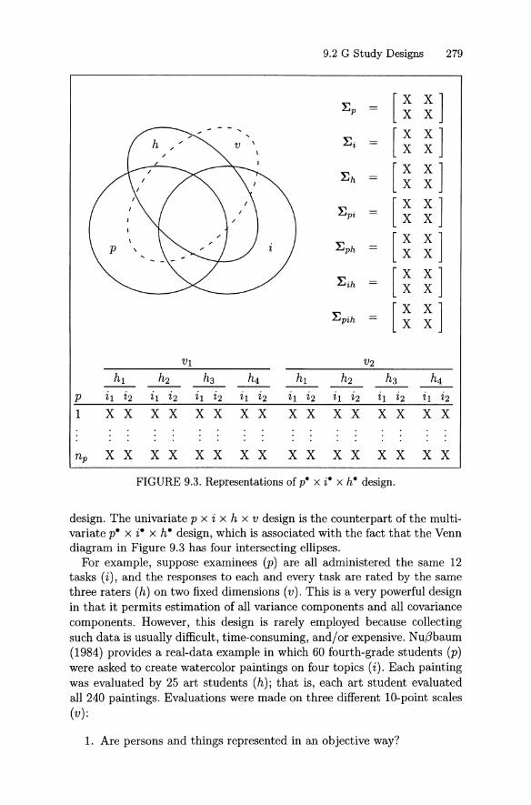
9.2 G Study Designs 279

E p [~ ~ ]E i [~ ~ ]Eh [~ ~ ]E pi [~ ~ ]E ph [~ ~ ]E ih [~ ~ ]

Epih [~ ~ ]VI V2

hl h2 h3 h4 hl h2 h3 h4

P il i2 il i2 il i2 i l i2 il i2 i l i2 i l i2 i l i21 X X X X X X X X X X X X X X X X

np X X X X X X X X X X X X X X X X

FIGURE 9.3. Representations of p. x i· x h· design.

design. The univariate p x i x h x V design is the counterpart of the multi ­variate p. x i- x h· design , which is associated with the fact that the Venndiagram in Figure 9.3 has four intersecting ellipses.

For example, suppose examinees (p) are all administered the same 12tasks (i), and the responses to each and every task are rated by the samethree raters (h) on two fixed dimensions (v) . This is a very powerful designin that it permits estim ation of all variance components and all covariancecomponents. However , thi s design is rarely employed because collect ingsuch dat a is usually difficult , time-consuming , and/or expensive. Nußbaum(1984) provides a real-data example in which 60 fourth- grade students (p)were asked to create wate rcolor paintings on four topics (i). Each paintingwas evaluated by 25 art students (h); that is, each art student evaluatedall 240 paintings. Evaluations were made on three different 10-point scales(v) :

1. Are persons and things represented in an objective way?

280 9. Multivariate G Studies

- - - - », [~~ ]

~i [~~ ]

~h = [X X]

~pi [~~ ]

~ph [X X]~ih = [X X]

[XX]~pih

i

I

I

I

\

\

v

-,

""I

1 XX XX XX XX XX XX XX XX

np XX XX XX XX XX XX XX XX

FIGURE 9.4. Representations of p. x i· x hO design.

2. Is the background appropriate?

3. Do relations between the objects become clear to the viewer?

For later reference, we refer to this as the Painting example .

p. x i· x hO Design

For the p. x i· x hO design different levels of h are associated with each ofthe fixed multivariate levels. Therefore, for each level of v there is a p x i x hvariance components design, and for each pair of levels of v there is a p x icovariance components design. Consequently, ~h, ~ph, ~ih, and ~pih arediagonal matrices; that is, each of the matrices involving h is diagonal.The univariate p x i x (h :v) design is the counterpart of the multivariatep. x i· x hO design, and the univariate counterpart is clearly associatedwith the the Venn diagram in Figure 9.4.

Brennan et al. (1995) provide a real-data example of this design in which50 examinees (p) each listened to 12 tape-recorded messages (i). Examinees

9.2 G Study Designs 281

were told to take notes while each message was played. At the conclusionof each message, examinees were told to use their notes to construct awritten message. The written messages were scored by trained raters ona five-point holistic scale for both listening skills and writing skills. Thelistening score reflected the accuracy and completeness of the informationprovided in the written messages. The writing score reflected other aspectsof the "quality" of the writing. There were two distinct sets of raters (h).Three raters evaluated the written messages for listening, and a differentthree raters evaluated the messages for writing. Subsequent ly, we refer tothis as the LW (i.e., Listening and Writing) example.

p. x iOx h· a n d p" x iOx hOD esigns

In terms of the LW example, if different t asks were used for listeningand writing, but the same raters were used for both dimensions, then thedesign would be p. x iO x h", This design has the same structure as t hep. x i · x hOdesign. The only difference between the two is that the rolesof i and h are interchanged.

Returning again to the LW example, suppose that different tas ks anddifferent raters were used for both listening and writ ing. Then the designwould be p. x iOx li" , and all matrices except ~p would be diagonal.

9.2.3 Two-Facet Nested Designs

For discussion purposes, it is convenient to group multivariate two-facetnested designs into those th at involve nesting with in the universe of admis­sible observations [pe x W:h·) , p. x W:h·) , and p. x (i0: hO) ], and thosethat involve nesting within the population of objects of measurement, whichare designated here as c for these designs [(p.: c") x i", (p.: c") x i", and(pO:c. ) x iO ].7

p. x W:h·) Design

For t he p. x W:h·) design, the variance components design is p x (i: h),the covariance components design is also p x (i :h), all five matrices arefull, and the univariate counterpart is p x (i:h) xv. Ret urning to the LWexample, suppose each of the three raters evaluated only four tasks, buteach rater provided bot h listening and writing scores. In this case, tasks (i)would be nested within raters (h), both tasks and raters would be crossedwith the fixed facet v, and the multivariate design would be p. x W:h·) .

7Strictl y sp eaking, of course, the obj ects of measurement are not identified until theD st udy and universe of generali zat ion are defined , but for discussion purposes here itis convenient to t hink of c as the objects of measurement .

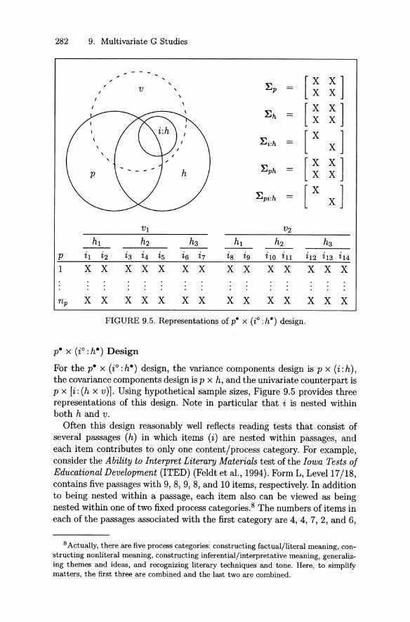
x x x x x x x x x x x x x x

FIGURE 9.5. Representations of p. x W:h· ) design.

p. x (io :h·) Design

For the p. x (io:h·) design, the variance components design is p x (i :h) ,the covariance components design is p x h, and the univariate counterpart isp x [i :(h xv)J. Using hypothetical sample sizes, Figure 9.5 provides threerepresentations of this design. Note in particular that i is nested withinboth hand v .

Often th is design reasonably weIl reflects reading tests that consist ofseveral passages (h) in which items (i) are nested within passages, andeach item cont ributes to only one content / process category. For example,consider the Ability to Interpret Litemry Materials test of the Iowa Tests 0/Educational Development (ITED) (Feldt et al., 1994). Form L, Level 17/18,contains five passages with 9, 8, 9, 8, and 10 items, respectively. In additionto being nested within a passage, each item also can be viewed as beingnested within one of two fixed process categories.f The numbers of items ineach of the passages associated with the first category are 4, 4, 7, 2, and 6,

8 Actually, there are five proc ess categories: constructing factual/literal meaning, con­struct ing nonliteral mean ing, const ructi ng inferential/interpret ative meaning, generaliz­ing t hemes and ideas, and recognizing Iiter ary techn iques and tone. Here, to simplifymatters , the first three are combined and the last two are comb ined.

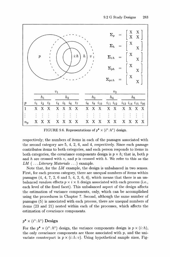
9.2 G Study Designs 283

~p [~ ~ ]\ ~h [ X

X]I \

, \

[ XX]

P I vI ~i:h =

\ I

[ XX]

\ I~ph

~pi :h [ XX]

vI v2

h1 h2 h3 h4 h5

P i 1 22 i3 i4 i5 i6 i7 i s ig i lO in i12 i13 214 it5 it6

1 X X X X X X X X X X X X X X X X

n p X X X X X X X X X X X X X X X X

FIGDRE 9.6. Representations of p. x W:hO) design.

respectively; the numbers of items in each of the passages associated withthe second category are 5, 4, 2, 6, and 4, respectively. Since each passagecont ributes items to both categories, and each person responds to items inboth categories, th e covariance components design is p x h; t hat is, both pand h are crossed with v, and p is crossed with h . We refer to this as theLM ( .. . Lit erary Materials . . . ) example.

Note th at , for th e LM example, the design is unbalanced in two senses.First, for each process category, there are unequal numbers of items withinpassages (4, 4, 7, 2, 6 and 5, 4, 2, 6, 4) , which means that th ere is an un­balanced random effects p x i x h design associated with each process (l.e.,each level of th e fixed facet) . This unbalanced aspect of the design affectsthe est imat ion of variance components , only, which can be accomplishedusing th e procedures in Chapter 7. Second, alt hough th e same numb er ofpassages (5) is associated with each process, th ere are unequal numbers ofitems (23 and 21) nested within each of th e processes, which affect s theest imat ion of covariance components.

p. x W:hO) Design

For the p. x (i° :hO) design, th e variance components design is p x (i :h) ,the only covariance components are those associated with p, and the uni­variat e counte rpart is p x (i :h :v). Using hypothet ical sample sizes, Fig-

284 9. Multivariate G Studies

ure 9.6 provides three representations of this design. Note in particularthat both i and h are nested within v.

Consider, for example, the Maps and Diagrams test of the Iowa Tests0/ Basic Skills (ITBS) (Hoover et al. , 1993). As the name suggests, inthis test there are two distinct types of stimulus materials: maps and di­agrams, Specifically, for Form K, Level 10, there are two maps and twodiagrams. For each of the two maps there are six and seven items, respec­tively; similarly, there are six and seven items, respectively, for each of thetwo diagrams. Subsequently, we refer to this as the MD (i.e., Maps andDiagrams) example.

Class-Means Designs: (p. :c·) x i·, (p.: c·) x i" , and (po: c") x iO

The (p. . c") x i·and (p. :c·) x iOdesigns can be viewed as "class-means"versions of the p. x i· and p. x iO designs, respectively. For the (p. :c") x i·design, as well as the (p.: c") x iO design, all persons (p) in all classes (c)take the same items (i). Furthermore, all persons and all classes contributedata to all levels of v, which means that :Ee and :Ep :e are full matrices.The only difference between these two designs is that the same items areassociated with each level of v for the (p. :c·) x i· design, whereas differentitems are associated with each level of v for the (p.: c") x iO design.

In most large-scale testing programs, the data collection procedure is onein which students are clearly nested within units (e.g., classes or schools),and all students take the same items . In this sense, the (p.: c") x i· and(p. :c") x iO designs are often a more accurate reflection of the realities ofdata collection than are the p. x i· and p. x iO designs. Usually, however,aggregations of persons are explicitly represented in designs only if D studyinterest will focus on the aggregated objects ofmeasurement (e.g., classes).

For the (po:c") x iO design, different groups of persons within each classrespond to different sets of items, and each group-set combination is associ­ated with only one level of v. In describing the design this way, it is impor­tant to note that neither "group" nor "set" is a facet. Rather these wordsare used simply to characterize random samples of persons and items, re­spectively. As such, the only full matrix is :Ee , and the design can be viewedas a matrix sampling version of the simple table of specifications model. Sel­dom, however, are different persons in the same class administered items inentirely different content categories; consequently, the (po :c") x iO designis rare.

9.3 Defining Covariance Components

A covariance component is the expected value of a product of two effects.Letting v designate random effects for variable v, and edesignate randomeffects for variable v' (v =1= v') , a covariance component for the effect o is

9.3 Defining Covariance Components 285

defined as

(9.16)

Consider, for example, the model equations for two levels, v and v', ofthe p. x W:h·) design:

and

X pihv ' = /.Lv' +ep + e h + e i :h + eph + epi :h ,

(9.17)

(9.18)

where the levels of i are different for v and v' . As discussed previously, theeffects within a level of the fixed facet are uncorrelated.? which means that

(9.19)

for a i' ß. Also,

(9.20)

for a i' ß·For the effects in Equations 9.17 and 9.18, there are three covariances

that are not necessarily zero--one for p, one for h , and one for ph. Thesecovariance components are denot ed

and

The covariance components for i :h and pi :h are both zero, because thelevels of i are different for v and v' in the p. x W:h·) design.!?

The definitions of covariance components are unaffected by whether aG study design is balanced or unbalanced. However , est imat ing covariancecomponents is much more complicated for unbalanced designs than for bal­anced ones. For that reason, est imat ion procedur es for unbalanced designsare treated later in Chapter 11.

9Most effects are necessar ily uncorrelated because of th e manner in which score effect sare defined in generalizability th eory.

lOCronb ach et al. (1972) would use different symbols to des ignate ite ms for the two lev­els (e.g., i for v and j for Vi), because th e items are indeed different for th e p. X (i0: h· )design. We do not follow this convent ion in this book, because generalizing this conven­tion to all designs that involve nesting leads to considera ble notational complexity.

286 9. Multivariate G Studies

9.4 Estimating Covariance Components fürBalanced Designs

It is important to understand the distinction between a balanced and anunbalanced covariance components design, as these terms are used in thisbook. Consider any two levels of a fixed facet. In the terminology of thisbook, to say that the covariance components design is balanced für thesetwo levels means that , for both levels of the fixed facet , t he variance compo­nents design is balanced. If t he variance components design involves nest­ing, it is not required that an equal number of condit ions be nested withineach of the two levels of the fixed facet . So, for example, if the variancecomponents design for each level of the fixed facet is p x (i :h) t hen n i mustbe a constant for each level of h within a particular level of v . However , n ineed not be the same for every level of v. For this reason , we somet imesuse n (with an appropriate subscript) to designate the G study sample sizefor one level of v, and m (with an appropriate subscript) to designate apossibly different sample size for a different level of v.

As an example of the distinction between balanced and unbalanced co­variance components designs, consider the p. x (i0 :h· ) design, and supposethere are five levels of v, each of which has nh = 2 levels of h (say, passages).Suppose further that the numbers of items associated with the two passagesfor each of the five levels of v are, respectively, 4/4, 4/4, 6/6, 3/5, and 2/6,where t he slash simply separates sample sizes. Any pairing of the first threelevels of v (Le., 1 with 2,1 with 3, or 2 with 3) const itutes a balaneed eovari­anee eomponents design in the terminology of this book, beeause th e twovariance components designs are balanced. Any pairing involving either ofthe last two levels of v eonstit utes an unbalanced covariance componentsdesign. Clearly, then, for the multivariate p. x (i0 :h· ) design, est imationof some of the covariance components may involve a balanced design, whileest imating others may involve an unbalanced design. As noted earlier , itis somewhat inaccurate to say that the multivariate p. x W:h· ) designinvolves the p x h covariance components design. Strictly speaking, thismultivariate design involves nv(nv - 1)/2 covariance components designsof the form p x h.

Für balanced multivariate designs with a single linked facet (e.g., thep. x iO design) , the observed covariance in Equation 9.7 is an unbiasedestimate of the covariance component for the linked facet. For balanceddesigns with more than one linked facet , we employ a procedure that isvery much like that used to est imate variance components for univariatebalanced designs. For such designs, Sections 3.3 and 3.4 provide equationsfor obtaining sums of squares, mean squares, and expected-mean-squareequat ions with respect to random effects variance components . Given theexpected-mean-square equations, it is straight forward to obtain est imatorsof the variance components for univariate balanced designs. A correspond-

9.4 Estimating Covariance Components 287

ing procedure discussed by Cronbach et al. (1972) can be used to obt ainestimators of covariance components when the covariance components de­sign is balanced. For this procedur e, sums of products (SP) replace sums ofsquares (SS) , mean products (MP) replace mean squares (MS) , expectedmean products (EMP) replace expected mean squares (EMS), and covari­ance components are est imated using the EMP equations. This methodfor est imat ing covariance components is also discussed by Bock (1975, pp.433ff.).

9.4.1 An Illustrative Derivation

Consider the p. x W:h·) multivariate design in which the covariance com­ponents design is p x h. The covariance components for :Ep , :Eh , and :Eph'respectively, are O"vv' (p), O"vv' (h) , and O"vv' (ph). Let us focus on est imatingthe covariance component for persons for levels v and v' of the fixed facet .The sum of products for persons is

SPvv,(p) = n<L (X pv - X v) (Xpv' - X v')p

= nhL XpvXpv' - npnhXvXv'p

= TPvv'(p) - TPvv'(/-L) ,

(9.21)

(9.22)

(9.23)

(9.24)

where the TP terms have obvious similarities with the T terms discussedin Section 3.3. The mean product for persons is

MD () _ SPvv,(p)"vv' p - 1 .np -

From Equations 9.24 and 9.22 it is evident th at the expected value of themean product for persons is

EMP•• ,(P) ~ np~ 1 [nh~ E (X""XP.' ) - npnhE (X. X u' )] , (9.25)

which depends on the expected value of two cross-product terms .To determine the first of these te rms, E (X pvXpv' ) , note that X pv is

simply the average over all levels of i and h of the observed scores forperson p on variable v . Similarly, X pv' is the average over all levels of i andh of th e observed scores for person p on variable v' . Formally,

Using Equations 9.17 and 9.18 in these expressions, we obtain

X - + + L h IJh + Lh Li IJi:h + Lh IJph + L hL i IJpi:hpv - /-Lv IJpnh nhni nh nhni

(9.26)

(9.27)

288 9. Multivariate G Studies

and

The expected value of the product of Equations 9.27 and 9.28, namely,E (X pvX pv' ), has 6 x 6 = 36 terms. Most of them are zero because, ingeneral ,

E (J.Lvea)

E (vaeß)

E (vaea)

= E (J.Lv'va) = 0,

o when a i= ß, and

o { when a is not an effect in thecovariance components design.

(9.29)

(9.30)

(9.31)

Note that Equation 9.31 implies that E (Vi:hei:h) = E (Vpi :hepi:h) = O.Since the possibly different values of ni and mi occur only in conjunctionwith the nested-effects terms in Equations 9.27 and 9.28, and since bothE (Vi:hei:h) and E (Vpi :hepi:h) equal zero, any difference between the val­ues of ni and m i has no effect on E (XpvX pv' ). This is a mathematicaldemonstration of the earlier statement that, if the multivariate design in­volves nesting, it is not required that an equal number of conditions benested within each of the levels of the multivariate fixed facet.

It follows from Equations 9.29 to 9.31 that

(9.33)

Each of the last two terms in Equation 9.32 expands into n~ terms, mostof which are zero. Specifically, (L:h Vh) (L:h eh) involves nh (nh - 1) termsof the form Vheh' (h i= h'), each of which has an expected value of zero.Similarly, (L:h Vph) (L:h eph) involves o« (nh - 1) terms of the form Vpheph'(h i= h'), each of which has an expected value of zero. These are two in­stances of the fact that

E ( e) 0 { when o and a' involve differ-Va o' = ent levels of the same effect.

It follows that Equation 9.32 simplifies to

fV - ) () avv,(h) avv,(ph)E \XpvXpV' = J.LvJ.Lv' + avv, p +--- + .

nh nh

A similar derivation for E (XvXv,) in Equation 9.25 gives

E (X X )_ avv'(p) avv,(h) avv,(ph)

v v' -J.LvJ.Lv'+--+--+ ,np nh npnh

(9.34)

(9.35)

9.4 Estimating Covariance Components 289

and replacing Equations 9.34 and 9.35 in Equation 9.25 leads to the finalresult for the expected mean product for persons:

(9.36)

In a corresponding manner it can be shown that the expected meanproduct for h is

and the expected mean product for ph is

EMPvv,(ph) = <7vv,(ph).

(9.37)

(9.38)

Replacing parameters with estimators in the expected mean product Equa­tions 9.36 to 9.38, it is easy to obtain the estimators of the covariancecomponents for the p x h covariance components design :

avv'(p)

avv,(h)

avv' (ph)

MPvv'(p) - MPvv,(ph)

nh

MPvv,(h) - MPvv,(ph)

(9.39)

(9.40)

(9.41)

9.4.2 General Equations

The form of Equations 9.36 to 9.38 is analogous to the expected-mean­square equations für the p x h design, and the form of Equations 9.39 to9.41 is analogous to equations for the estimated random effects variancecomponents for the p x h design. That is, covariance components in EMPequations playa role that parallels that of variance components in EMSequations. Indeed, general equations for estimating covariance componentsfor balanced multivariate designs closely parallel the general equations inSection 3.4 for estimating random effects variance components for a uni­variate design .

For any component 0: in the covariance components design.l! the sum ofproducts is

SPvv'(O:) = 7l"(ä) LXQ V XQ V ' ,

Q

(9.42)

where X Q V and X Q V ' are deviation scores of the type discussed in Sec­tion 3.3.2, the summation is taken over all indices in 0:, and the multiplier

11 It is important to note that the Cl' terms involved here are those for the covariancecomponents design only.

(9.43)

290 9. Multivariate G Studies

{

the product of the sample sizes for all7l"(ä) = indices in the covariance components

design except those indices in o .

For the p. x (iO :h·) multivariate design in which the covariance compo­nents design is p x h, Equation 9.21 is an instance of Equation 9.42. Forthe same design, another instance is

SPvv,(ph) = L L (Xphv - X pv - x.; + Xv)p h

X (Xphv' - X pv' - Xhv' + Xv'). (9.44)

Since SPvv'(a) in Equation 9.42 is a product of deviation scores, it canbe called the corrected sum of products, as opposed to the uncorrected sumof products that is usually easier to compute:

{

7l"(ä)LXovXov'TPvv,(a) = 0

7l"(all)XvXv'

if ai J.l

if a = J.l,

(9.45)

where 7l"( alt) is the product of the sample sizes for all indices in the covari­ance components deslgn.P To express any SP term with respect to a setof TP terms, the algorithm in Section 3.2.3 can be used, with SP termsreplacing SS terms, and TP terms replacing T terms: Also, using the samereplacements, for one- and two-facet designs, Appendix A provides SPterms with respect to a set of TP terms.

For the p. x (io :h·) multivariate design in which the covariance compo­nents design is p x h, Equation 9.23 expresses SPvv,(p) with respect to TPterms. For the same design, SPvv'(ph) in Equation 9.44 can be expressedas

SPvv,(ph) = TPvv,(ph) - TPvv'(p) - TPvv ,(h) + TPvv'(J.l).

The mean product for a component a is simply

(9.46)

Making use of the zero expectations given by Equations 9.29, 9.30, 9.31,and 9.33, it can be shown that the expected value of the mean product for

127l"(a) has been used previously in Equation 3.9 to designate the corresponding quan­tity for variance components designs.

13In this chapter occasionally Cl< is permitted to represent J1. as well as the effects associ­ated with covariance components. This notationalliberty is adopted to avoid introducingadditional notational conventions.

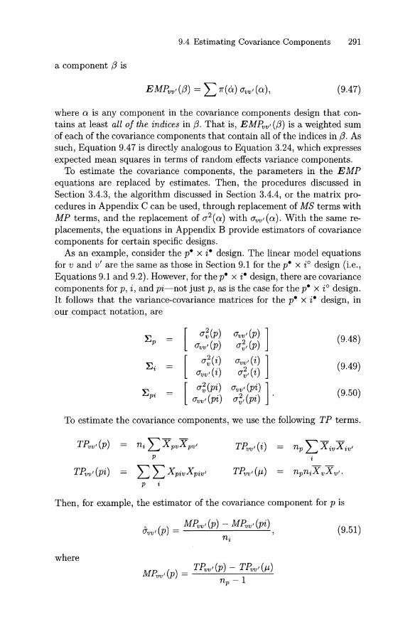
9.4 Estimating Covariance Components 291

a component ß is

(9.47)

where a is any component in the covariance components design that con­tains at least all 01 the indices in ß. That is, EMPvv'(ß) is a weighted sumof each of the covariance components that contain all of the indices in ß. Assuch, Equation 9.47 is directly analogous to Equation 3.24, which expressesexpected mean squares in terms of random effects variance components.

To estimate the covariance components, the parameters in the EMPequat ions are replaced by estimates. Then, the procedures discussed inSection 3.4.3, the algorithm discussed in Section 3.4.4, or the matrix pro­cedures in Appendix C can be used, through replacement of MB terms withMP terms , and the replacement of 0"2(a) with O"vv ,(a). With the same re­placements, the equat ions in Appendix B provide estimators of covariancecomponents for certain specific designs.

As an example, consider the p. x i· design. The linear model equationsfor v and v' are the same as those in Section 9.1 for the p. x iOdesign (i.e.,Equations 9.1 and 9.2). However, for the p. x i · design, there are covariancecomponents for p, i, and pi-not just p, as is the case for the p. x iOdesign.It follows th at the variance-covariance matrices for the p. x i· design, inour compact notation, are

:Ep [O"~(p)

O"vv'(p)

[O"~ (i)

O"vv' (i)

[O"~ (pi)

O"vv' (pi)

O"vv' (p) ]O"~, (p)

O"vv,(i) ]0";,(i)

O"vv' (pi) ]O"~ , (pi) .

(9.48)

(9.49)

(9.50)

To est imate the covariance components, we use the following TP terms.

TPvv,(pi)

ni LXpvXpvl

p

L L XpivXpiv'P

Then, for example, the est imator of th e covariance component for p is

(9.51)

where

MP. ()- TPvv'(p) - TPvv'(p,)

vv' p -np -1

292 9. Multivariate G Studies

TABLE 9.3. Synthetic Data Example für Balanced p. x i · Design

VI V2

P i l i2 i3 i4 i5 i6 il i2 i3 i4 i5 i6 x., Xp2 Xp l Xp2

1 6 4 3 5 4 4 6 4 5 6 4 5 4.3333 5.0000 21.66672 3 2 2 4 5 5 6 4 5 6 2 5 3.5000 4.6667 16.33333 6 5 7 5 4 3 6 5 8 4 6 3 5.0000 4.8333 24.16674 4 2 2 3 3 5 5 4 2 4 3 5 3.1667 3.8333 12.13895 4 4 3 5 4 6 4 5 5 3 3 7 4.3333 4.5000 19.50006 8 5 4 7 5 4 9 6 6 5 7 7 5.5000 6.6667 36.66677 5 4 5 7 4 4 4 5 6 7 4 5 4.8333 5.1667 24.97228 4 5 3 4 5 6 6 7 6 6 5 6 4.5000 6.0000 27.00009 7 5 4 6 6 5 6 7 3 5 5 6 5.5000 5.3333 29.333310 5 3 3 7 4 5 6 5 4 6 2 6 4.5000 4.8333 21.7500

Sum 52 39 36 53 44 47 58 52 50 52 38 55 45.1667 50.8333 233.5278

X l = 4.5167 TPI 2(p) = 1401.1667 TPI2(pi) = 1441.0000X2 = 5.0833 TPI2 (i) = 1385.7000 TPI2(f.L) = 1377.5833

M p[ 3.4611 2.6204 ] Ep [ .3682 .3193 ]

2.6204 3.7500 .3193 .3689

M i [ 4.6967 1.6233 ] E i [ .3444 .0919 ]= 1.6233 4.7367 .0919 .3200

M pi[ 1.2522 .7048 ] :Epi [ 1.2522 .7048 ]= .7048 1.5367 .7048 1.5367

and

MPuu,(pi) =TPuu'(pi) - TPuu'(p) - TPuu,(i) + TPuu'(f.L )

(np - 1)(ni - 1)

Note, in particular, that for both the p. x iO and the p. x i· designs,the definition of the covariance component for p is given by Equation 9.6,but the estimators are different for the two designs. For the p. x iOdesign ,the estimator is simply the observed covariance in Equation 9.7. For thep. x i · design, the estimator is O"uu'(p) in Equation 9.51, which involves thedifference between two mean products.

Table 9.3 provides a synthetic data example of the computations requiredto estimate variance and covariance component s for the p. x i · design .This synthetic data set is for 10 persons and six items, with two levels of afixed facet . The bottom of the t able provides the mean-squares-and-mean­product matrices (Mp , Mi, M pi) in which the diagonal elements are meansquares and t he off-diagonal elements are mean products. The esti mated

9.4 Estimating Covariance Components 293

varia~ce and covariance components are provided in the matrices ~p, ~i ,

and ~pi'

9.4.3 Standard Errors 0/Estimated Covariance Components

Estimated covariance components are subject to sampling variability, ofcourse, but very little has been published about this topic. One resultdiscussed by Kolen (1985, p. 215) and based on Kendall and Stuart (1977,p. 250) is that, if Y and Z have a bivariate normal distribution, then forsamples of size n,

(9.52)

We cannot use this result directly for our purposes here because, amongother things, it is expressed in terms of parameters rather than the esti­mators discussed in this chapter. However, the form of Equation 9.52 isevident in the expression discussed below for the estimator of the standarderror of an estimated covariance component.

For v and v' , let us assume that corresponding effects have a bivariatenormal distribution, and different effects are uncorrelated. For the p. x i·design, this means that (vp, ~p), (Vi, ~i)' and (Vpi' ~pi) have bivariate normaldistributions; and

for a i ß. Under these assumptions, using procedures discussed by Searle(1971, pp . 64-66), an approximate estimator of the standard error of anestimated covariance component is

(9.53)

where ß indexes the mean products that enter o-vv,(a) , and ll'(ä) is givenby Equation 9.43. Note that when v = v', o-[o-vv,(a)] in Equation 9.53 isidentical to Equation 6.2 for the estimated standard error of an estimatedvariance component for a random model.

For the p. x i· design, o-vv' (p) is a linear combination of MPvv'(p) andMPvv,(pi) (see Equation 9.51), and o-[o-vv,(p)] is

MSv(p)MSv' (p) + [MPvv' (p)]2 + _M_Sv.:.....:(pt""·-:-)M_S-'-v,-.:.::(p-;-'i)c-+--'[:-M;-Pv_v,-;:(p--'i)-=-]2n;[(np - 1) + 2] n;[(np - l)(n t - 1) + 2]

(9.54)For the synthetic data in Table 9.3, it is easy to verify that o-[o-vv ,(p)] = .227.

(9.55)

294 9. Multivariate G Studies

The standard error in Equ at ion 9.54 is interpretable as the standarddeviation over replications of o-vv'(p ) = [MPvv'(p) - MPvv,(pi)Jlni, whereeach such estirnate is obtained for a different randorn sample of np personsand ni iterns frorn the population and universe. For each replication, ifthe square of the quantity in Equation 9.54 were obtained , t he expectedvalue over replications of these squared quantities would be the variance ofo-vv' (p).

A special case of Equation 9.53 arises for balanced mult ivariat e designswith a single linked facet , say p. Under the assumpt ions of bivariat e nor­rnality and uncorrelated effects, an est imate of the standard erro r of o-vv' (p)is

S;(p) S;,(p) + [Svv,(p)J2(np - 1) + 2

where S; (p) and S;, (p) are unbiased estimates of the variances of X pv andX pv', respectively, and Svv' (p) = o-vv'(p) is the observed covariance. Forthe p. x iOdesign ,

and

For other designs with a single linked facet , different expressions apply forS;(p) and S;,(p) in terms of est imate d variance components, but Equ a­tion 9.55 still applies .

It is evident frorn the form of Equ ation 9.53 that est imated standarderrors of esti rnated covariance components tend to be large when the esti­mate involves many mean prod ucts, when the cornponent mean squares andrnean products are large, when degrees of freedorn are smalI, and /or whenrr(ß) is srnall. Recall from Section 6.1.1 that est imated standard errors ofest irnate d variance cornponents tend to be large under sirnilar conditions.

In general, the estirnat ed standard erro r of an est imate d covariance com­ponent can be smaller or larger t han the est imated standard erro rs for t heassociated est irnate d variance components; not at ionally, o- [o-vv' (a)] can besmaller or larger than 0- [0-;(a)] or 0- [0-;,(a)]. However, unde r some circurn­st ances, relative magnitudes can be predicted. For example, when rneanproducts are srnall relative to mean squares, est irnated standa rd errors forestirnated covariance components (Equation 9.53) tend to be smaller thanfor estimated variance cornponent s (Equ ation 6.1).

Also, when variance components are equal , standard errors for est imate dcovariance cornponents tend to be smaller than for est imated variance com­ponents. This can be inferred by comparing Equation 9.52 for var[o- (Y, Z)]and the corresponding equat ion for the variance of the est imates of variance(see Kolen , 1985 , p. 215) :

var[o-2 (y)] = 2(j4(Y)/n . (9.56)

Suppose that (j2(y) = (j2(Z). Since corr( Y,Z ) ::; 1, it necessarily followsthat (j(Y, Z) ::; (j2(y) and, therefore, (j2 (y, Z ) ::; (j4(y ). Adding (j4(y ) to

9.5 Discussion and Other Topics 295

bot h sides of this inequality gives

Dividing both sides by n leads to the conclusion that

var[a-(Y, Z)] ::; var [a-2 (y )].

Of course, this result is dependent on normality assumpt ions.

9.5 Discussion and Other Topics

The MP procedure discussed in this chapter for est imat ing covariance com­ponents with balanced designs is directly analogous to the ANOVA pro­cedure for est imat ing variance components that was extensively discussedin ear lier chapte rs. The MP procedure is essent ially the procedure pro­posed by Cronb ach et al. (1972) over a quarter century ago. Implementa­t ion of the MP procedure is relatively st ra ightforward, and t he proceduremakes no assumpt ions about distributional form. Other procedures mightbe considered, however. For example, the "variance of a sum" procedurediscussed later in Section 11.1.5 can be used to obtain maximum likelihoodand MINQUE estimates of covariance components for some designs. Also,structural equation modeling might be used to estimate at least some ofthe covariance components in a multivariate design.

9.5.1 Interpreting Covariance Components

As discussed in Section 9.3, a covariance component is the expected valueof t he product of two effects . This is equivalent to the expected value of t hecovariance of the two effects , since the expected value of the effects them­selves is zero. In interpreting est imates of covariance components, thesedefinitional issues are central.

For multivariate designs with a single linked facet , the interpretat ionof a covariance component is especially straightforward: it is simply thecovariance between universe scores for the v and v' levels of that facet .Furthermore, t he observed covariance is an unbiased est imate of the co­variance component. For designs with more th an one linked facet , however ,it is crucial to note th at observed covariances are not direct estimates ofcovariance components for th e population and universe.

Let us ret urn to the synt hetic dat a example of the multivariate p. x i ·design in Tab le 9.3. The MP est imates of the covariance components arethe lower diagonal elements of the following matri ces, and the MB est imatesof the variance components are the diagonal elements :

[.3682.3193

.8663 ].3689

(9.57)

296 9. Multivariate G Studies

:Ei [ .3444 .2767 ] (9.58)= .0919 .3200

:E pi [1.2522 .5081 ] (9.59).7048 1.5367 .

One way to interpret estimated covariance components is in terms of theestimated disattenuated correlations based on them. These are reported initalics in the upper-diagonal positions of the three matrices. For example,the estimated correlation between universe scores for persons on v and Vi

is

(9.60).3193 = .8663.y' .3682 x .3689

A () o-vv' (p)Pvv' P = J' 2 ( ) ' 2 ( )(Tv P (Tv' P

In words, Vp and ~p are correlated about .87. (The reader can verify that theobserved-score correlation for persons is .73, which is not to be interpretedas an estimate of the disattenuated correlation for persons .)

Similarly, the estimated disattenuated correlation for i is

.0919 = .2767,y' .3444 x .3200

(9.61)

and the estimated disattenuated correlation for pi is

A ( ') o-vv' (pi)Av' pi = J'2( ') '2 ( ')(Tv pt (Tv' pi

,7048 = .5081.y'1.2522 x 1.5367

(9.62)

The positive values of these two disattenuated correlations suggest thatcorrelated error will be an issue in D study results.

Transforming estimated covariance components into disattenuated cor­relations occasionally leads to the uncomfortable occurrence of correlationsgreater than unity. This can occur as a result of sampling error and, ofcourse , it is more likely to occur when sample sizes are smalI. Also, corre­lations greater than unity can be indicative of one or more hidden facets inthe G study design. For example, suppose occasion is a facet in the universeof admissible observations, but occasion is not explicitly represented in theG study design. Suppose also that the data for estimating variance compo­nents were obtained on one occasion, and the data for estimating covariancecomponents were obtained on a different occasion. Then, disattenuated cor­relations greater than unity may result solely because v and Vi effects aremore highly correlated for the "covariance-components occasion" than forthe "variance-components occasion." In short, a disattenuated correlationgreater than unity does not mean the computations are incorrect although,of course, that's always a possibility!

Variance components are necessarily non negative, although ANOVA es­timates of them can be negative due to sampling variability. By contrast,covariance components can be negative, so a negative estimate is not neces­sarily indicative of sampling variability. Even so, in particular studies, there

9.5 Discussion and Other Topics 297

may be good reason to believe t hat one or more covariance components (i.e. ,parameters) should be positive, and t he occurrence of a negative est imate isprobably attributable to sampling variability. In such cases, should a nega­tive est imate be set to zero in the G study? This aut hor thinks not. Even ifthe est imate is negative, the investigator seldom knows for certain that theparameter is positive. Furthermore, using the procedures discussed in thischapte r , the est imate is unbiased, and changing it to zero makes it biased.It is probably not prudent to set a negative est imate to zero, at least notuntil D st udy issues are considered.

Throughout t his chapter, we have assumed that the st ruct ure of the uni­verse of adm issible observat ions and t he G st udy are t he same. Of course,t his need not be t he case. Suppose, for example, t hat t he population anduniverse of admissible observatio ns have the st ructure p. x i · x li". The Gstudy design might have the st ruct ure p. x W: h· ). If so, in addition toconfounded variance components, the G study involves confounded covari­ance components in the sense that

andlYvv,(pi :h) = lYvv,(pi) + lYvv,(pih) ,

(9.63)

(9.64)

where covariance components to t he left of t he equalit ies are for the Gst udy p. x (iD: h· ) design, and t hose to the right are for t he p. x i · x h·popul ation and universe of admissible observat ions. Th ese relationshipsparallel those discussed in Section 3.2.1 for variance components .

As noted above, hidden facets can occur in multivariat e G studies. Again ,suppose that the population and universe of admissible observations havethe structure p. x i · x h· , where h stands for occasion. The G st udy mighthave the p. x i · design and, if so, occasion would be a hidden facet. In t hiscase, assuming t he data were all collected on a single occasion,

lYvv' (plp· x i ·)

lYvv,(i lp· xi·)

lYvv' (pilp· xi·)

lYvv' (p) + lYvv'(po)

lYvv,(i) + lYvv,( io)

lYvv' (pi) + lYvv' (pio),

(9.65)

where covariance components to the left of the equalit ies are for the G studyp. x i · design , and those to the right are for the p. x i · x h· populationand universe of admissible observations. These relationships par allel thosediscussed in Section 5.1.4 for variance components .

9.5.2 Computer Programs

In t he author's opinion, one very real impediment to the use of multivariat egeneralizability t heory has been that applicat ion of t he theory requiresexte nsive computat ions t hat are often not readily performed with available

298 9. Multivariate G Studies

compute r programs/packages. To ameliorate this problem, the compute rprogr am mGENOVA discussed in Appendix H was designed specificaIly formultivariate generalizability theory as discussed in this book. mGENOVAest imat es variance and covariance components for each of the designs inTable 9.2, except the last one, t he (po:c") x iO design.

Input for mGENOVA consists of a set of cont rol cards along with a dataset . The data layout at th e bot tom of the figures in Section 9.2 mirrorsthat employed by mGENOVA. The algorit hms used by mGENOVA are notmatrix-based; consequently, mGENOVA can process an almost unlimitednumb er of observations very rapidly. mGENOVA provides G study out putof the type discussed in this chapte r, as weIl as D study out put of the typediscussed in subsequent chapters.

For balanced multivariat e designs, various compute r packages often canbe used to perform some or aIl of the computations. For example, in theappendix to their overview of multivariate generalizability theory, Webbet al. (1983) provide a discussion and example of how th e SAS GLM andMATRlX procedures can be used to est imate covariance components basedon the MP procedure in Section 9.4.2. SAS IML could be used , as weIl.

9.6 Exercises

9.1* For the APL Survey discussed in Section 3.5.4, Table 3.7 report st hat t he est imated variance components for the southern region, fora univariate mixed model with content categories fixed, are:

a2(plV ) = .0378,a2(i:v lV ) = .0259,

a2 (pvlV ) = .0051,a2 (pi:vlV) = .1589.

(Here we use v and V rather than h and H .) The correspondingvariance-covariance matrices für the multivariat e p. x iOdesign are:

.0342 .0332 .0298 .0353

.0332 .0409 .0386 .0463

.0298 .0386 .0408 .0348

.0353 .0463 .0438 .0548

.0290 .0342 .0345 .0423

.0208.0298

.0364.0081

.0290

.0342

.0345

.0423

.0386

00343 1

9.6 Exercises 299

.1334.1634

~pi .1618.1593

.1765

Use the elements ofthese matrices with Equations 9.12 to 9.15 to ver­ify the results reported above for the variance components o-2(alv).Why is it that o-2(vlV)= .0013 in Table 3.7 does not arise as somecombinat ion of elements in the multivariate variance-covariance ma­trices?

9.2* For the p. x iO x hOdesign, provide the Venn diagram, design matri­ces, and record layout .

9.3 For the (p. :c") x iO design, provide the Venn diagram, design matri­ces, and record layout . For the record layout assurne there are twoclasses with three and two persons per dass, respectively; assurnethere are 6 items in VI, and 14 items in V2 .

9.4* For the p. x i· design and the synthet ic data in Table 9.3, verify thenumerical results for the TP t erms, the MP terms, and the est imatedcovariance components.

9.5* If the synthetic dat a in Table 9.3 were for a p. x iO design, whatwould be o-vv' (p)?

9.6 Suppose the synthetic data in Table 9.3 were for the i · :p. design.Determine the rnean-squares-and-rnean-products rnatrices and thevariance-covariance matrices.

9.7* For th e p. x i · design in Table 9.3, est imate the standard errors ofthe est imated covariance components for i and pi.

9.8 For the p. x i · design in Table 9.3, the est imated variance compo­nents for p are nearly equal. It was stated in Section 9.4.3 that thest and ard error of an est imated covariance component will be smallerthan the standard error of the variance components when the vari­ance components are equal. Verify that thi s statement applies to theest imates in Table 9.3.

9.9* Miller and Kane (2001) discuss a pretest-posttest study in which eachof 30 students took the same 15-item test on two occasions. The 15items were subdivided into five categories (c) of three items (i) each.The pretest, post tes t , and difference-score randorn effects variancecomponents are:

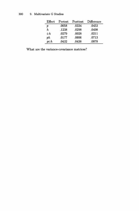
300 9. Multivariate G Studies

Effect

Phi :hphpi :h

Pretest.0058.1238.0279.0177.0432

Posttest.0334.0298.0028.0606.0438

Difference.0453.0498.0211.0713.0878

What are the variance-covariance matrices?

10Multivariate D Studies

This chapter is split into two major parts followed by a few real-data exam­ples. Section 10.1 covers fundamental issues about multivariate universesof generalization and D studies. Section 10.2 treats a selected set of otherissues that, in most cases, are probably less central than the issues coveredin Section 10.1. All of the issues, and most of the results and procedures,discussed in this chapter apply to both balanced and unbalanced multivari­ate D study designs . However, attention is focused primarily on balanceddesigns in the sense that, for each of the fixed levels in the D study, thereis a balanced variance components design. Multivariate unbalanced designsare the subject of Chapter 11.1

10.1 Universes of Generalization and D Studies

Letting T designate the objects of measurement "facet," in multivariategeneralizability theory, for each T there are n v universe scores }.Lrv, eachof which is associated with a single level of the fixed facet. In this sense,there is a universe score profile for each T . The universe score (for an objectof measurement) for any particular level of the fixed facet is the expectedvalue over alt facets in the universe of generalization for that level (and that

1 A number of issues covered in this chapter are not treated by Cronbach et a l. (1972) .

302 10. Multivariate D Studies

object of measurement). Unless otherwise specified, it is always assumedhere that, for each fixed condition of measurement, all facets are random.

Parts of this section are, in effect, an extension of the Jarjoura andBrennan (1982, 1983) multivariate p. x JO table of specifications modelto more complicated multivariate designs. The initial parts of this sectionrepeat some of the introduction to multivariate generalizability theory inSection 9.1.

10.1.1 Variance- Covariance Matrices for D Study Effects

A multivariate D study analysis is, in asense, a conjunction of n v univariaterandom model analyses that are linked through covariance components. Byway of illustration, let us consider the p. x r design. The linear modelequations for levels v and v' are:

andX pv' = XpIv' = /-Lv' + ~p +6 + ~pI,

with the following three D study variance-covariance matrices,

(10.1)

(10.2)

(10.6)

}jp [ a;(p) avv'(p) ] (10.3)avv'(p) a;,(p)

}jI = [ a;(I) avv'(I) ] (10.4)17vv,(I) 17~, (I)

}jpI [ 17;(pI) 17vv'(pI) ] (10.5)avv,(pI) a;,(pI) .

As in Chapter 9, the fact that these matrices are represented using onlytwo rows and two columns does not mean that there are only two levels ofthe fixed facet. This compact form simply indicates the notation used torepresent the elements of the matrices.

For balanced designs, multivariate D study analyses in the mean scoremetric are performed using procedures that are directly analogous to thosediscussed in Chapter 4 for univariate random models. That is, letting ädesignate the indices for a particular D study effect,

2 _ a;(a)av(a) = (-I)'

7fv orr

where

and

= {the product (for v) of the D study sam­ple sizes für all indices in ä except Tj

(_) avv,(a)

avv, a = (-I) ,7fvv' aT

(10.7)

(10.8)

10.1 Universes of Generalization and D Studies 303

where

_ { the product (for v and v') of the D study1I'vv,(a lr ) = sampie sizes for all indices in ä except r . (10.9 )

Recall that D study condit ions are the same for linked effects, and linkedeffects produce nonzero covariance components . It follows that the D studysampie sizes for v and v' are the same for a nonzero covariance component .So, for example, for th e balanced p. x r design, (Jvv,(I) = (Jvv , (i)/n~ and(Jvv,(pI) = (Jvv,(pi)/n~.

Unless otherwise noted, all results in this chapte r are in the mean scoremetric. To obtain D study variance-covariance matrices for the total scoremetric , cert ain rules can be followed. First , to obtain the elements of all Dstudy matrices except ~T ' use 1I'v(älr) and 1I'vv,(älr) as multipliers, ratherth an divisors , of G study variance and covariance components , respectively.Second , transform the elements of ~T as folIows,

where 11'v and 11'v' are t he total number of D study condit ions sampled forv and v', respect ively. These sample sizes are the same as those for thehighest order interaction, for designs with single observations per cell,

10.1.2 Variance-Covariance Matrices for Universe Scores andErrors 0f Measurem ent

Given the variance-covariance matrices for D study effects, it is easy to usethem to express variance-covariance matri ces for profiles of universe scores(~T), relative errors ( ~o), and absolute errors (~b. ). Rules for doing so aredirectly analogous to those discussed in Chapter 4 for univariate randommodels. In particular ,

~T {variance-covariance matrix(10.10)= for universe scores for r

~o {sum of all ~ö such that ä includes r(10.11)

and at least one other index

~b. sum of all ~ö except ~T ' (10.12)

So, for example, for the p. x J. design, these rules lead to the followingmatrices

~p

~pI

~I + ~pI '

(10.13)

(10.14)

(10.15)

304 10. Multivariate D Studies

For any multivariate design, the elements of :Er> :Eo, and :Eb, are varianceand covariance components , as indicated in the following representationsof the matrices.

=

(10.16)

(10.17)

(10.18)

Again, this compact form for representing the matrices does not necessarilymean that nv = 2.

Note that the relative-error and absolute-error covariance componentsin :Eo and :Eb" respectively, are directly analogous to relative-error andabsolute-error variance components . For example, for the p. x I· design,

) ()r7vv' (pi)

r7vv' (o = r7vv' pI = I 'n i

and

) ()r7vv' (i) r7vv' (pi)

r7vv' (Ö) = r7vv,(I + r7vv' pI = --,- + I .n i n i

Often, it is convenient to transform relative-error and absolute-error co­variance components to thei r correlated error counterparts; that is,

(10.19)

and,(Ö) _ avv' (Ö ) ( )

Puv - Jr7~(Ö)r7~,(Ö) 10.20

One of the distinct advantages of multivariate generalizability theory isthat the off-diagonal elements of :Eo and :Eb, provide explicit indicatorsof different types of correlated error. In most other measurement theories,correlated error is assumed not to exist , is confounded with other effects ofinterest , or lurks in statist ical shadows.

As in univariate theory, the expected value of the observed variance forobject-of-measurement mean scores for v is

(10.21)

which we sometimes abbreviate ES; (r ). Similarly, the expected value ofthe observed covariance between object-of-measurement mean scores for vand v' is

(10.22)

10.1 Universes of Generalization and D Studies 305

which we sometimes abbreviate ESvv,(r) . It follows that the observed co­variance is an unbiased estimate of the universe score covariance only whenrelative errors are uncorrelated, as they are for the p. x JO design.

Note that Equation 10.21 is the expected value of a variance and Equa­tion 10.22 is the expected value of a covariance. Unbiased estimators ofthese quantities are the observed variance for v, and the observed covari­ance for v and v', respectively. With persons as the objects of measurement,a matrix display of these estimators is

s [S;(p)

Svv,(p)SSv~r ((p)) ] ,

v' p(10.23)

or, more succinctly,

10.1.3 Composites and APriori Weights

Occasionally, ~T' ~ö, and/or ~c. contain the primary (or even the sole)statistics of concern. This might occur, for example, when profiles of uni­verse scores are of principal concern. More frequently, however, some com­posite of universe scores is of interest. In general, we define a compositeuniverse score as

(10.24)

where the W v are weights defined apriori by an investigator.f Sometimesthey are called nominal weights.

Usually these apriori, or nominal, weights are defined such thatL:v W v = 1 and W v ~ 0 for all v. A common example is W v = niv/ni+,where ni+ designates the total number of items over all levels oE the fixedfacet. In this case, the weights are proportional to the number of items inthe measurement procedure that are associated with each Vj if items arescored dichotomously, the composite is the proportion of items correct.

The theory discussed here, however, does not require that L:v W v = 1.For example, when nv = 2, difference scores can be obtained by settingW v = 1 and W v' = -1 . Also, sometimes all weights are set to unity. Thiscommonly occurs when expressing the composite in the total score metric(see Exercise 10.1).

Composite universe score variance is a weighted sum of the elements in~T :

(Yb(r) L w~(Y~(r) + L L wvwv'(Yvv,(r)v v#v'

(10.25)

2The use of the term "a priori" here is unrelated to the use of that term in thediscussion of MINQUE(O) in Seetion 7.3.1.

306 10. Multivariate D Studies

= LLWvWvIO'vvl(r) .v v'

(10.26)

Equation 10.26 follows from Equation 10.25 because O'vv,(r ) = O'~(r) whenv = v' .

The fact that the W v are used to define composite universe score in no wayrequires that they be used to estim ate composite universe score. However ,usually the W weights are employed to obtain the following estimator ofcomposite universe score,

For this est imator, relative error variance for the composite is

O'b(o) = LLwvwvl O'vvl(o) ,V v'

(10.27)

(10.28)

where O'vv'(0) = O'~ (0) when v = v' . Similarly, absolute error variance forthe composite is

O'b(ß) = L L WVWV' O'vvl(ß) ,V v'

(10.29)

where O'vv,(ß) = O'~(ß) when v = v' .A multivariate generalizability coefficient can be defined as the ratio of

composite universe score variance to itself plus composite relative errorvariance:

O'b (r ) + ab (0)

L v L v' WvWv' O'vv ,(r )

(10.30)

(10.31)

Similarly, a multivariat e phi coefficient can be defined as the ratio of com­posite universe score variance to itself plus composit e absolute error vari­ance:

=

O'b(r) + O'b(ß)

L v L v' WvWv' O'vvl(r )

(10.32)

(10.33)

10.1.4 Composites and Effective Weights

It is evident from the form of Equ at ions 10.25 and 10.26 that different levelsof the fixed facet can have different cont ribut ions to composite universe

10.1 Universes of Generalization and D Studies 307

score variance . In particular, for level v, the proportional contribution is

n v

Wv L Wv' (Jvv'(T)ewv ( T) = _...:.v_'=...:l~,.....,....__

(Jb(T)(10.34)

which means that I:v eWv(T) = l.In terms of distinctions discussed by Wang and Stanley (1970), the

eWv(T) play the role of effective weights, whereas the Wv play the role ofnominal weights .f In the context considered here, nominal weights expressthe investigator's judgment about the relative importance of the variouslevels of the fixed facet in specifying the universe of generalization. Ef­fective weights, which are based in part on nominal weights, reflect therelative statistical contribution of a particular level of the fixed facet . It isclear from Equation 10.34 that effective weights and nominal weights arenot usually the same.

Effective weights can be defined also with respect to composite relativeerror variance and/or composite absolute error variance:

and

Clearly, the effective weights ewv(T), ewv(0), and ewv(tl) usually will bedifferent. There is no comparable trilogy for w weights. That is, w weightsrelate to universe scores, only-not errors of measurement.

10.1.5 Composites and Estimation Weights

Usually the nominal W v weights are used not only to define compositeuniverse score (Equation 10.24) but also to estimate it (Equation 10.27).Sometimes, however, other weights, say av , are used for estimation pur­poses. In this case,

XrCla = LavXrv;v

(10.35)

and mean-squared error involved in using X rCla as an estimate of compos­ite universe score is

MSEc(tl) - 2E[XrCla - fLrcJ

[~(a" -W")~.r31n much of the iiterature, this distinction is drawn with respect to composite ob­

served score variance, rather than composite universe score variance.

308 10. Multivariate D Studies

v v'

+ LLavav'O"vv,(ß),v u'

(10.36)

where O"vv,(ß) is based on the D study sample sizes used with the av. Notethat there is a nonnegative contribution to MSEc(ß) from the elementsof :ET and from the means of the fixed categories (J.Lv ) '

For tests developed according to a table of specifications, a reasonablequestion to consider is the extent to which the fixed category system, andthe assignment of specific numbers of items to categories, leads to a re­duction in some measure of error. After all, if no such reduction occurs, itwould be prudent to reconsider the need for the particular category system.One way to address this question is to compare a-b(ß) to MSEc(ß) whenMSEc(ß) is based on assigning all items to only one of the n v categories.Obviously, there are nv such comparisons, and they are likely to give dif­ferent answers. Even so, this somewhat ad hoc examination of the efficacyof a category system can be useful (see Jarjoura & Brennan, 1982, 1983,for a real-data example) .

Also, it can be useful to examine MSEc(ß) for sample sizes slightlydifferent from those actually used with a measurement procedure. This cangive an investigator a sense of how important it is that all instances of themeasurement procedure (e.g., forms) use exactly the same sample sizes.

Under some circumstances, it may be appropriate to consider mean­square relative error:

v v'

+ LLavav'O"vv,(8) .v v '

(10.37)

For example, if test forms are carefully equated, it might be judged sensi­ble to assurne that :E6 = :Ea and the profile of JLv is constant over forms, atleast approximately. Under these assumptions, MSEc(ß) in Equation 10.36becomes MSEc(8) in Equation 10.37.

10.1.6 Synthetic Data Example

Consider, again, the synthetic data example for the p. x i· design in Ta­ble 9.3 on page 292. In this data set the G study sample size for items isni = 6. If the D study sample size is n~ = 8, then

[.3682 .3193].3193 .3689

[.0431 .0115].0115 .0400

10.1 Universes of Generalization and D Studies 309

:Ep [ [.1565 .0881 ].0881 .1921 .

RecaIl, as weIl, that the G study has observed means of X I = 4.5167 andX z = 5.0833.

Using Equations 10.13 to 10.15, the estimates of the universe score, rel­ative error, and absolute error matrices are

:Er [ .3682 .8663 ] (10.38).3193 .3689

:Eo [ .1565 .5081 ] (10.39).0881 .1921

:EL', [ .1996 ·4627 ] (10.40).0996 .2321 .

The upperdiagonal elements in italics are correlations. That is, the esti­mated correlations between universe scores, relative errors, and absoluteerrors are Puv,(r) = .8663, Puv,(6) = .5081, and Puv'(~) = .4627, respec­tively. Note, in particular, that correlated 6-type error is greater than cor­related ~-type error even though the 6 covariance is smaIler than the ~covariance (see Exercise 10.4 for a condition under which this inequalitycan occur) . Note also that the observed-score variance-covariance matrixthat would be expected with n~ = 8 is

s = [.5247 .7509].4074 .5610 '

(10.41)

where the upper diagonal element is the expected observed score correla­tion.

For the sake of specificity, suppose VI represented accuracy and Vz rep­resented speed in solving math word problems administered by computer.In specifying the universe of generalization, an investigator might judgethat accuracy is three times more important than speed. This would implythat for this investigator's universe WI = .75 and Wz = .25. Under theseassumptions, composite universe score variance is estimated to be

&b(r) = (.75)( .75)( .3682) + (.25)( .25)(.3689) + 2(.75)(.25)(.3193) = .3499.

If examinee reported scores are obtained by weighting accuracy threetimes as much as speed, then the estimation weights are the same as theW weights, the estimate of composite relative error variance is

&b(6) = (.75)(.75)( .1565) + (.25)( .25)(.1921) + 2(.75)(.25)( .0881) = .1331,

the 6-type signal-noise ratio is 2.63, and the multivariate generalizabilitycoefficient is Epz = .724.

310 10. Multivariate D Studies

Under the same assumptions, the estimate of composite absolute errorvariance is

8"b(ö.) = (.75)(.75)(.1996) + (.25)(.25)(.2321) + 2(.75)(.25)(.0996) = .1641,

the ö.-type signal-noise ratio is 2.31, and ~ = .681. The proportional con­tribution of accuracy to composite absolute error variance is estimated tobe

(A) _ .75[.75( .1996) + .25(.0996)] _ 7 9

eWI L.l - .1641 - . 97 ,

which means that accuracy contributes about 80% and speed contributesabout 20% to composite absolute error variance .

These results assurne that the apriori weights and the estimation weightsare the same. By contrast, suppose a second investigator decided to giveequal weight to accuracy and speed in arriving at examinee reported scores,but wanted to interpret these reported scores as estimates of the universeof generalization characterized by the original w weights. In this case, themean-square error in using .5XpI + .5X p2 as an estimate of .75J.lpl + .25J.lp2is

MSEc(Ö.) = [(.50 - .75)4.5167 + (.50 - .25)5.0833]2

+ [(.50 - .75)2.3682 + (.50 - .25)2.3689

+ 2(.50 - .75)(.50 - .25).3193]

+ .25[.1996 + .2321 + 2(.0996)]

= .1839,

which is about 12% larger than composite absolute error variance (.1641)that is based on using the w weights as estimation weights.

10.2 Other Topics

The topics in Section 10.1 are essential to understanding D study issuesin multivariate generalizability theory, but there are numerous other rel­evant topics . One such topic is multivariate unbalanced designs, which isthe subject of Chapter 11. Also, Chapter 12 provides a relatively lengthytreatment of multivariate regressed scores. A few additional topics are cov­ered less extensively in this section . To keep the treatment somewhat lessabstract, the notation and discussion here use persons (p) as the objects ofmeasurement. As always, however, any facet could constitute the objectsof measurement.

10.2.1 Standard Errors 01 Estimated Covariance Components

Section 9.4.3 discussed a normality-based approach to estimating standarderrors of estimated G study covariance components that are linear combi-

10.2 Other Topics 311

nations of mean products. When the D study covariance components arelinear functions of the G study components, the D study components arealso linear combinations of the mean products. Under these circumstances,an approximate estimator of the standard error of an estimated covariancecomponent is

(10.42)

where ß indexes the mean products that enter O'vv,(a), and f(ßla) is the co­efficient of MPvv'(ß) in the formula for O'vv' (a). The only difference betweenEquation 10.42 for D study covariance components and Equation 9.53 forG study covariance components is that f(ßla) in Equation 10.42 plays therole of 1/1T'(&) in Equation 9.53.

The more general formulation in Equation 10.42 permits it to apply toany estimator that is a linear function of the mean products. In particu­lar, this equation applies to estimates of universe score covariance compo­nents, relative error covariance components, and absolute error covariancecomponents-for levels of a fixed facet and for composites. For example,for the p. x P x H· design

where

and

O'vv' (8) = O'vv' (pI) + O'vv' (pH) + O'vv' (pI H) , (10.43)

A ,( IH) = MPvv,(pih)avv p I I .ninh

It follows that an expression for O'vv' (8) in terms of mean products is

O'vv' (8) =

(10.44)

where the terms in the three sets of parentheses are f(piI8) , f(phI8), andf(pihI8), respectively.

Therefore, using Equation 10.42, the estimated standard error of O'vv' (8)is

312 10. Multivariate D Studies

10.2.2 Optimality Issues

To the extent possible, when a composite is under consideration, it is sen­sible to choose sample sizes that minimize composite error variance, givenwhatever other constraints may exist. A relatively simple example is choos­ing D study sample sizes for the p. x JO design under the assumption thatn~+ = Lv n~v is fixed (see Jarjoura & Brennan, 1982). For this design,assuming the estimation weights equal the apriori weights, composite ab­solute error variance is

Since the D study sample sizes n~v are positive integers , iteration might beused to minimize aß(ß). This approach to minimization is defensible to theextent that precise estimates of the variance components are available . Ifthe estimates are imprecise , then any minimization claim based on iterationis suspect, at best.

However, if precise estimates are available, a simpler solution involvesthe following inequality,"

l: w~ [a;(i) ~ a;(Pi)]v nw

> ~ [l: wvJa~(i) + a~(pi)] .nH v

Minimization of aß(ß)occurs when

(10.46)

although the resulting n~v are not necessarily integers. Ta obtain integervalues for practical use, it is possible to iterate around the solution inEquation 10.46.

4This inequality is based on the Cauchy-Schwartz Inequality.

10.2 Other Topics 313

For the synthet ic dat a example introduced in Table 9.3 on page 292, sup­pose th e D st udy design is p. x JO with W l = .75 and W 2 = .25. If th e totalnumb er of items is const rained to be n~+ = 10, th en using Equ ation 10.46the opt imal sam ple sizes are

n~ l = 1O(.75)y!.3444 + 1.2522 = 7.3559.75y!.3444 + 1.2522 + .25y!.3200 + 1.5367

and

1O(.25)y!.3200 + 1.5367n~2 = = 2.6441.

.75y1.3444 + 1.2522 + .25 y1.3200 + 1.5367

Using n~l = 7 and n~2 = 3 gives o-b(~) = .167, and using n~l = 8 andn~2 = 2 gives o-b(~) = .170. Consequently, th e optimal integer samplesizes are seven and three.

This approach to determining sample sizes th at minimize O"b(~) can beexte nded to other, more complicated multivariate designs. Furthermore,constra ints such as cost can be employed instead of, or in addit ion to ,fixing total sample sizes (see, e.g., Marcoulides & Goldstein, 1990, 1992).However , t he logic of multivariate generalizability theory as presented inthis book requir es that the ui; weights be specified a priori, and any sta­t istical procedure that modifies these weights a posteriori is at odds withthis perspective on th e theory. In particular , a statistical procedure de­scribed by Joe and Woodward (1976) for choosing weights that maximizea generalizability coefficient is inconsistent with the logic of multivariategeneralizabili ty th eory presented here. In effect, this procedure producesa set of a poste riori category weights th at may have little to do with therelative importance of the catego ries for the prespecified intended use ofthe measurement procedure.

Although the ui; need to be specified a priori, it is certainly possible fortwo investigators to use the same measurement procedure for different pur­poses, which may well require different weightings of the fixed categories,that is, different values for th e W v . Also, in the early stages of defining auniverse of generalizat ion and deciding on th e relative importance of thevarious categories, it may be very helpful to use various statistical proce­dures, as well as other sources of information, to make an informed choiceof the W v weights. Indeed, at this formative stage, the Joe and Woodward(1976) procedure might be useful. Note, also, th at it is possible to spec­ify effective weights and determine the W v from th em (see Dunnette &Hoggat t , 1957, and Wilks, 1938).

The W v are an integral part of th e specificat ion of an investigator's uni­verse of generalization, which provides at least par t of the definition of t heconst ruct of interest to the investigator. As such, th e W v are fixed, andth ey apply not only to the measurement procedure that generat es a par­ticular set of data, but also to all other randomly parallel inst ances of the

314 10. Multivariate D Studies

measur ement procedure in the universe of generalization. Any optimizationprocedure that treats the W v as random is likely to yield different valuesfor the ui; depending on which instance of the measurement procedure isemployed; and there is no guarant ee that any of these different sets of val­ues for the W v will accurately reflect t he investigator's judgments about therelative importance of the categories. So, any opt imization procedure thattr eats the W v as random effectively creates a moving validity target for in­ferences based on the measurement procedure. In the end, the W c must bespecified before any meaningful st atements can be made about error vari­ances, generalizability coefficients, and so on; and the investigator must beprepared to provide some type of validity defense for the W v values.

10.2.3 Conditional Standard Errors of Measurement forComposites

Section 5.4 discussed conditional standard errors of measurement for bal­anced designs in univariate generalizability theory. As discussed there,a(Ll p) is the standard error of the mean for the within-person D studydesign associated with person p. So, for example, if the across-persons uni­variate D study design is p x I , then the within-person design for eachperson is simply I, and a(Llp) is the standard error of the mean for theperson's item scores.

This logic is easily extended to multivariate designs. Assuming the esti­mat ion weights (av ) and the a priori weights (w v ) are the same, absoluteerro r for the composite is

LlpC X pC - J.Lpc

= L Wv (Xpv - J.Lpv)v

L Wv Llpv'v

It follows immediately that the condit ional absolute-error SEM is

ac(Llp) = L w~ a~(Llp) + L L WvWv' avv'(Llp),v v # v '

where2 -av(Llp) = var(X pv - J.Lpvlp)

is the variance of the mean for person p on v , and

is the covariance of person p's mean scores on v and V'.

(10.47)

10.2 Other Topics 315

TABLE 10.1. Synthetic Data Example of Conditional Absolute Standard Errorsof Measurement for Balanced p. x r Design with n; = 6 and W l = W2 = .5

Actual Fitted"p X p 1 X p2 X pC af(llp ) a~(llp) a12(llp) ac(llp) ac(llp)

4 3.1667 3.8333 3.5000 .2278 .2278 .1722 .4472 .42512 3.5000 4.6667 4.0833 .3167 .3778 -.1000 .3516 .44515 4.3333 4.5000 4.4167 .1778 .3833 .1000 .4362 .45401 4.3333 5.0000 4.6667 .1778 .1333 .1000 .3575 .4594

10 4.5000 4.8333 4.6667 .3833 .4278 .2167 .5578 .45943 5.0000 4.8333 4.9167 .3333 .6278 .4333 .6760 .46397 4.8333 5.1667 5.0000 .2278 .2278 .1722 .4472 .46528 4.5000 6.0000 5.2500 .1833 .0667 .0000 .2500 .46859 5.5000 5.3333 5.4167 .1833 .3111 .1000 .4167 .47016 5.5000 6.6667 6.0833 .4500 .3111 .1333 .5069 .4729

Mn 4.5167 5.0833 4.8000 .2661 .3094 .1328 .4586b .4586b

afitted uc(Llp ) = J- .0187 + .0822 X pc - .0066 X~c .bSquare root of the avetage of t he variances.

These varian ces and covariances can be conceptualized in the followingmanner. Any particular inst ance of the measurement pro cedure will resultin mean scores on v and VI for the person . The variance of the person 'smean scores for v over replicat ions of the measurement procedure is a;(llp).The covariance of these mean scores for v and VI over replications of themeasurement pro cedure is avv,(llp).

The condit iona l relative-errot SEM can be approximated as

(10.48)

The correct ion to aß(llp) in Equation 10.48 is simply the difference be­tween the overall absolute and relative error variances for the composite.The logic behind using this constant correct ion for all persons mirrors thatdiscussed in Section 5.4 for univariate designs .

Consider again the syntheti c dat a example for the p. x J. design in Ta­ble 9.3 on page 292. Assuming the G and D study sample sizes are thesame (n i = n~ = 6) and the apriori weights for the two variables are equal(Wl = W 2 = .5), Table 10.1 provides conditional absolu te-error SEMs forcomposite scores, for each of the 10 persons , with persons ordered fromsmallest to largest observed composite score. Let us focus on person num­ber one (the fourth person from the top of Table 10.1). The raw scores ,means , variances, and covariance for this person are:

316 10. Multivariate D Studies

TABLE 10.2. Synthetic Data Within-person t- x r" and T- x RODesigns

VI V2

t rl r2 r3 rl r2 r3

1 3 2 2 2 3 3~ [ .0741 .2235 ]E t

2 3 3 2 4 4 4 .2235 .2926

3 3 3 3 4 4 4Er [ .0333

.2148 ]=4 3 3 3 3 3 45 2 2 1 2 3 1 [ .3000

.3852 ]6 1 3 3 2 4 3 E tr =

7 2 3 2 2 4 48 3 3 2 2 4 3

E~p [ .0285 .0224 ]9 3 3 2 2 4 3 .0224 .1137

10 3 3 3 4 4 4

Mean 2.6 2.8 2.3 2.7 3.7 3.3

i l i 2 i3 i 4 i 5 i 6 Mean Var Cov

VI 6 4 3 5 4 4 4.3333 1.0667.6000

V2 6 4 5 6 4 5 5.0000 .8000

It follows thato-n~~ l ) = 1.0667/6 = .1778,

o-~(ßl) = .8000/6 = .1333,

o-12(ßd = .6000/ 6 = .1000,

and the est imated conditional absolute-error SEM for person one's com­posite score is

&c(ßI) = ) .25(.1778) + .25(.1333) +2(.25)(.1000) = V.1278 = .3575.

Table 10.1 also provides fitted values for the condit ional absolute-errorSEMs, or, more correctly, the square roots of the quadratic-fits for theconditional absolute-error variances. These are obt ained in th e same man­ner as discussed in Section 5.4 for univariate designs. Note also that theoverall absolute-error SEM can be obtai ned from the conditional values:specifically,

o-c(ß) = 110L o-b(ß p ) = .4586.

p

As another example, suppose the G study design is p. x t· x r"; the Dstudy design is p. x T· x R O, and the G and D study sample sizes are thesame with nt = n~ = 10 tasks and nr = n~ = 3 raters. Table 10.2 provides

10.2 Other Topics 317

hypothetical data for a particular person in the design. Note that the Gstudy design for this person (and all other persons in this design) is te x r" ,and the D study design is Te X RO.

Table 10.2 also provides the three G study estimated variance-covariancematrices for this particular person. For these data, the estimated variance ofthe mean (over 10 tasks and three raters) for VI is the conditional absolute­error variance:

o-r(t) o-r(r) o-r(tr)--+--+--n~ n~ n~n~

.0741 .0333 .300010+-3-+30.0285.

Similarly, for V2,

'2(1:::. ) _ .2926 .2148 .3852_(72 p - 10 + 3 + 30 - .1137.

The estimated conditional absolute-error covariance is simply

Note that (7I2(r) and (7I2(tr) are not present in (7I2(l:::.p ) because they areboth zero for the te x t" design.

These conditional absolute-error variance and covariance components arethe elements of !:D.

pin Table 10.2. Using Equation 10.47 with WI = W2 = .5,

conditional absolute-error variance for the person's composite score is

o-c(l:::.p ) = ).25(.0285) + .25(.1137) + 2(.25)(.0224) = V.0467 = .2162.

Other examples of conditional SEMs for multivariate composites are pro­vided by Brennan (1996a, 1998).

10.2.4 Profiles and Overlapping Confidence Intervals

It is relatively common practice for test publishers to produce score reportsin which a confidence interval is placed around each score in a person 'sprofile of n v test scores. Almost always the width of each interval is twostandard errors of measurement, and the person is usually told somethinglike, "If any two intervals for your scores overlap, then your level of achieve­ment for the two tests is likely the same." This common practice raises anumber of quest ions about overlapping confidence intervals. Here we focuson only two of these questions and develop results based on classical testtheory. We then extend and express these results in terms of multivariate

318 10. Multivariate D Studies

generalizability theory. It is especially important to note that the resultsderived here require normality assumptions.f

Let two tests be denoted X and Y with standard errors of measurement ofaEx and aEy, respectively. Under normality assumptions, 68% confidenceintervals are X ± aEx and Y ± oe-, with endpoints of (XL, X H) and(YL,YH), respectively. Consider a particular person whose true scores onboth tests are the same. For such aperson, the probability that the twointervals will not overlap is

Pr(no overlap) = Pr(XL > YH) + Pr(XH < YL). (10.49)

Since Pr(XL > YH) = Pr(XH < YL), we derive Pr(XL > YH) and thendouble it to obtain the result . To begin,

Pr(XL > YH) Pr(XL - YH > 0)Pr [(X -aEx) - (Y +aEy) > 0]

= Pr(X - Y > aEx +aEy),

which essentially translates the original question about "no overlap" to aquestion ab out the distribution of observed difference scores. Let us assurnethat observed difference scores are normally distributed, under the usualclassical test theory assumption of uncorrelated errors of measurement.Since we are assuming that TX = Ty, the normality assumption is

where a~x +a~y is the variance of the difference in the error scores, whichequals the variance of the observed difference scores. It follows that

Doubling this result we obtain

[ (os +aE )]Pr(no overlap) = 2 1 - Pr z< x y ,

Ja2 +a2Ex Ey

(10.50)

5The classical test theory aspects of this section are based largely on an exercisedeveloped by Leonard S. Feldt .

10.2 Other Topics 319

with its complement being

(

(JE +(JE )Pr(overlap) = 2 x Pr z< x yV(J2 + (J2E x Ey

-1. (10.51)

The probabilities in Equations 10.50 and 10.51 are based on the assump­t ion of uncorrelat ed error, with intervals formed by adding and subtractingone stand ard error of measurement to a person's observed scores on X andY. Also, of course, these prab abiliti es have been derived under the classicaltest theory assumpt ion of undifferentiated errar .

These results are easily extended to designs and situat ions accommo­dated in multivar iate generalizability theory. For example, for each v, 100/,%intervals might be formed with respect to overall absolute error as folIows,

(10.52)

where z(l+'Y )/2 is the z-score associated with a two-sided 100/,% confidenceinterval. Under these circumstances, for a person with the same universescore on v and v',

where the denominator is the standard error of the observed differencescores, which can be denoted (JD(~) '

Equation 10.53 has the same form as Equation 10.51, but there are dis­similar ities. Most importantly, the stand ard error of the difference scoresincorporates the possibility of correlated absolute error." All other thingsbeing equal, large positive values for correlated error lead to larger proba­bilities of overlap than small positive values. In thi s sense, if correlated errorwere present but ignored, th e prab ability of overlap would be understat ed.

Of course, Equation 10.53 simplifies if correlated error is not present(e.g., the p. x JO design), but even th en Equat ion 10.53 differs from theclassical test theory result in Equation 10.51, in that Equation 10.53 isbased on absolute error, whereas Equat ion 10.51 uses the error in classicaltheory. These two types of error may or may not be the same, dependingon the design. For example, if the design is p. x JO

, absolute error and theerror in classical theory are different ; if the design is JO

: p" , absolute errorand classical error are the same.

The probability of overlap result in Equation 10.53 is based on the as­sumption th at the person's universe scores are equal; that is, J." pv - J."pv ' = O.Without this rest riction, we obtain a more general form of Equation 10.53.

6Less importantly, Eq ua tio n 10.53 is stated for any confidence coefficient , whereasEqu ati on 10.51 ap plies as stated for a con fidence coefficient of .68 only.

320 10. Multivariate D Studies

Specifically, for a prespecified value for the difference in universe scores(f..Lpv - f..Lpv' ), the probability that two 100,% intervals will overlap is

Pr(overlap) =

{

Z(1+')')/2 [O"v(ß) + O"v,(ß)] - (f..Lpv - f..Lpv,)}Pr z< -

JO"~(ß) + O";,(ß) - 20"vv,(ß)

{

-z(1+')')/2 [O"v(ß) + O"v' (ß)] - (f..Lpv - f..Lpv') }Pr z < . (10.54)

JO"~(ß) + O";,(ß) - 20"vv,(ß)

Obviously, intervals such as those given in Equation 10.52 and 10.54 canbe expressed in terms of overall relative standard errors of measurement,which leads to probability of overlap equations identical to Equations 10.53and 10.54 except that 0 replaces ß . Similarly, conditional absolute or rel­ative standard errors of measurement can be used.

As an example , consider the p. x r design with n~ = 6 using the sYE­thetic data in Table 9.3 on page 292. Dividing each of the elements in :Eiand iSp i by six, and then summing the elements gives

[.2661 .1328 ].1328 .3094 .

The standard errors for the two levels are c71(ß) = ).2661 = .5159 andc72(ß) = ).3094 = .5563, and the standard error of the difference scores is

t:TD(.6.) = } .2661+ .3094 - 2(.1328) = .5567.

The two 68% confidence intervals are X p1 ± .5159 and X p2 ± .5563. Underthe assumption that f..Lpl = f..Lp2, the probability that these two intervals willoverlap is

Pr(overlap) = 2 x Pr ( < .5159 + .5563) 1z .5567 -

2 x Pr (z < 1.9260) - 1

2 x (.9730) - 1

= .946.

10.2.5 Expected Within-Person Profile Variability

When profiles are under considerat ion, usually interest focuses on individ­ual persons , as discussed in Section 10.2.4. To characterize the ent ire mea­surement procedure for a population, however , we can consider expectedwithin-person profile variability, which we denote generically as V(*). Forexample, V(Xp ) is the expected within-person profile variability for ob­served scores, and V(JLp ) is the expected within-person profile variabilityfor universe scores.

10 .2 Other Topics 321

The V(*) forrnulas discussed in this section result from the well-knownanalysis of variance identity. For a row-by-column matrix, the analysis ofvariance identity guarantees that the average variance within the columnsplus the variance of the column means equals the "total" variance, and,similarly, the average variance within the rows plus the variance of the rowmeans equals the "total" variance. Letting Ypv be scores for any variable,

1""2 - [ ] 2-- L..J o (Ypv ) + var(~) = E p var(Ypv ) + o (r;),n v v v v

where "var" designates variance over the fixed levels of v. The quantityE p [var(Ypv ) ] is a measure of the average variability of the profile of Yscores, which we designate simply as V(Yp ) . It follows from the aboveequation that

(10.55)

Of course, if var(Ypv ) is computed for each p in the data, then the averagewill be an estimate of V(Yp ) . This direct computational estimate, however,is not always practical, or even possible, because it requires that the entireset of Ypv data be available.

Variance Formulas

Applying Equation 10.55 to raw scores X pv for a finite number of personsgives"

(10.56)

It is important to note that S~(p) is the average over the nv observedvariances, and Svv,(p) is the average over alt n~ elements of the observedvariance-covariance matrix, which includes those with v = v'. The multi­plicative factor (np -1) /np has no compelling theoretical relevance or likelypractical importance, but it does guarantee that the value obtained usingthis formula is identical to the value obtained through directly computingthe average of the variances of the n p profiles for a finite number of persons.Of course, this multiplicative factor approaches unity as np ---* 00.

Consider, again, the synthetic data example for the p. x I" design withn~ = 6. The person mean scores and related statistics and matrices, in­cluding the observed score variance-covariance matrix, are provided in Ta-

7St r ict ly speaking, this equation is expressed in terms of estimators, since, for exam­pIe, S~(p) and Svv' (p) have been defined previously as estimators.

322 10. Multivariate D Studies

TABLE 10.3. ObservedProfile Variability for Synthet ic Data Example of p. x rDesign with n; = 6

P X p 1 Xp2 Mean Vara

1 4.3333 5.0000 4.6667 .11112 3.5000 4.6667 4.0833 .3403 iSp [ .3682 .3193 ]3 5.0000 4.8333 4.9167 .0069 .3193 .36894 3.1667 3.8333 3.5000 .1111 [ .2087 .1175 ]5 4.3333 4.5000 4.4167 .0069 :Eo .1175 .25616 5.5000 6.6667 6.0833 .3403

[7 4.8333 5.1667 5.0000 .0278 :EA.2661 .1328 ]

8 4.5000 6.0000 5.2500 .5625 .1328 .3094

9 5.5000 5.3333 5.4167 .0069 S [ .5769 .4367 ]= .4367 .625010 4.5000 4.8333 4.6667 .0278

Mean 4.5167 5.0833 4.8000 .1542Var '' .5192 .5625 .4669 .0337

a Biased est imates.

ble 10.3.8 For these data, the average of the observed variances is

S:(p) = .5769 ; .6250 = .6010,

the average of all elements in the S matrix is

S () - .5769 + .6250 + 2(.4367) - 5 88vv' p - 4 -. 1 ,

and the vari ance (biased est imate ) of the two means (4.5167 and 5.0833)is .0803. It follows that observed-score profile variability is

V(X p ) = .9(.6010 - .5188) + .0803 = .1542,

which is identical to the value reported in Table 10.3 based on direct com­putation of the average of the observed profile variances for the 10 persons.

For this synthet ic dat a example, direct computat ion cannot be employedfor any other design or sample size, because the observed scores for ot herdesigns and sample sizes are not known. However , Equ ation 10.56 can beused. So, for example, with n~ = 8, Equ ation 10.41 provides the expectedobserved variances and covariances, which leads to

V(X p ) = .9(.5428 - .4751) + .0803 = .1412.

8Nüte that the variances in S are unbiased esti mates , wher eas th e "Var" estimatesar e biased. Für example, (1O/9)( .5192) = .5769.

(10.57)

10.2 Other Topics 323

For universe-score profile variability, applying Equation 10.55 gives

np -1 2V(JLp ) = --[O'v(p) - O'vv/(p)] + var(JLv)'

n p

For the synthetic data example, th e elements of the ~p matrix are givenin Table 10.3. The average of the two variances is .3686, the average ofall four variance-covariance elements is .3439, an est imate of var(JLv) isvar(Xv) = .0803, and the universe-score profile variability is

V(JLp ) = .9(.3686 - .3439) + .0803 = .1024.

Since universe scores are unknown, this result cannot be obtained throughdirect computation using persons' universe scores. We retain the multi­plicative factor (np - l)/np solely for purposes of consistency with otherV(Xp ) .

The variance of the 8-type errors for a randomly selected person is

(10.58)

where we have dropped the (np - l)/np multiplicative factor . For the syn­thetic data with n~ = 6, V(op ) = .058. Consequently, the st andard devia­tion of the 8-type errors of measurement for a typical person is ,,1.058 = .24.In a corresponding manner, we can express the variance of the ß-type er­rors for a typical person as

(10.59)

which is V(ßp ) = .078 for the synt het ic data with n~ = 6.

Relative Variability

As in univariate theory, it is natural to consider functions of variabilities,particularly ratios. One such ratio is

(10.60)

which is the proportion of the variance in the profile of observed scores fora typical person that is explained by the varian ce in the profile of universescores for such aperson. If V(JLp ) is viewed as a measure of the flatness

of the profile of universe scores, and V(Xp ) is viewed as a measure of theflatness of the profile of observed scores, then Q is a measure of the relativeflatness of these profiles for a typical person.

Q is also interpretable approximately as a type of generalizability coef­ficient for a randomly selected person p. For a specified person , we can

324 10. Multivariate D Studies

define a person-level generalizability coefficient as the ratio of var(/1pv) tovar(Xpv), where the variance is taken over levels of v. Obviously, this ratiois not estimable for a given person, because universe scores are unknown.The expected value, over persons , of this ratio would be the expected gen­eralizability coefficient for a randomly selected person. We approximatethis expected value over persons with the ratio of the expected values inEquation 10.60.

For the synthetic data with n~ = 6, g = .1024/.1542 = .664, whichsuggests that, for a typical person, 66% of the variance in observed meanscores for the n v variables is attributable to variance in universe scores. Forthe synthetic data with n~ = 8, g= .1024/ .1412 = .725.

It is important to note that these variability formulas are for profiles­not composites. As such, apriori (w) weights and estimation (a) weightsplay no role. Also, it is helpful to remember that throughout this sectionwe have been viewing data from the within-person, or "row," perspective.By contrast, when we consider one of the nv x nv matrices such as :Ep, weare viewing data from a "column" perspective. The measures of (relative)profile variability discussed here provide overall or summative results forthe measurement procedure, or average results for a typical person. Theyshould not be construed as capturing all the information in the data. Inparticular, the variance and covariance components should be examinedand reported always.

10.2 .6 Hidden Facets

Hidden facets can occur in multivariate generalizability theory, just as theycan in univariate generalizability theory. Obviously, the fact that a facetis hidden makes it easy to overlook. Less obviously, the consequences offailing to recognize a hidden facet can be seriously detrimental to inter­pretations. Often, a hidden facet is effectively fixed, and the likely conse­quences involve underestimating error variances, overestimating universescore variances, and severely overestimating coefficients. These conclusionsare like those discussed previously for univariate analyses, but multivariateanalyses involve the additional complexities of covariance components andattention to composites.

Suppose, for example, that the universe of generalization is best repre­sented by the multivariate p. x JO x H· structure, which means , of course,the H is a random facet in the universe of generalization. However, whenthe G study data were collected, suppose the same single level of h wasemployed with all p, i , and v . In this case, undoubtedly the investigatorwill analyze the G study data according to the p. x iO design, and theestimated variance and covariance components will be estimates of

», + :Eph = [O"~(p) + O"~(ph)

O"vv' (p) + O"vv' (ph)

~i + ~ih

~pi + ~pih

[[

10.2 Other Topics 325

2 (') + 2 ( 'h) ] (10.62)av' t av' t

2 ( ' ) + 2 ( 'h) ] . (10.63)av ' pi av' tn

Note that none of the elements of ~h is present in any of these threematrices. This is certainly one sense in which h is "hidden."

Now, suppose these p. x iO estimated variance and covariance cornpo­nents are used to estimate relative error variances for the categories andthe composite. Further, suppose the G and D study sample sizes are thesame, which means, among other things, that the investigator really wantsnh = 1 for decisions based on the measurement procedure. Clearly, niv

will divide not only the pi variance components but also the pih variancecomponents, which is what the investigator intends. However, estimates ofthe ph variance components will be absent from estimates of all relativeerror variances. This will result in underestimates of relative error variancefor each universe score.

If the w weights are all nonnegative, the absence of the ph variance com­ponents from the category error variances will also lead to underestimatingthe composite relative error variance . In addition, the composite relativeerror variance will be underestimated even more because of the absence ofthe avv , (ph), assuming the avv , (ph) are positive. If some of the avv , (ph) arenegative and/or some of the w weights are negative (e.g., when the com­posite is a difference score), composite relative error variance is stilllikelyto be biased, but the direction of the bias would have to be determined ona case-by-case basis.

The same conclusions discussed in the previous paragraph apply to ab­solute error variances, as well, By contrast, universe score variances for thecategories and the composite will tend to be overestimated, because theywill include the ph variance components. For composite universe score vari­ance there is an additional inflation factor caused by the presence of theavv , (ph), assuming the avv , (ph) and the w weights are positive . The con­junction of underestimating error variances and overestimating universescore variance willlikely lead to dramatic overestimates of coefficients. Ex­ceptions to these conclusions will occur only if the variance componentsinvolving h are negligible; or, in the case of the composite, possibly if someof the avv , (ph) andfor the W v are negative.

In beginning this discussion of hidden facets, we assumed that each ob­servation involved the same single level of the h facet . This is probably themost frequent way a hidden facet arises. The same logic would apply, how­ever, if each observation in the p. x iO design were a mean over the samenh levels of the h facet . Notationally, we would represent this difference byusing pH rather than ph in Equations 10.61 through 10.63. We are not sug­gesting it is necessarily good practice to collapse observations over a facetin this manner. We are merely noting that an analysis of such collapsed

326 10. Multivariate D Studies

data effectively treats H as fixed, which produces biased estimates if theintent is that H be random,

The occurrence of hidden facets is much more common than generallyrealized . To ascertain whether hidden facets are present, an investigatormust clearly specify the intended universe of generalization. If the D studydesign does not explicitly represent all facets in the universe of general­ization, then one or more facets are hidden . Probably the most frequentlyencountered hidden facet is "occasion." Very often, an investigator's in­tended universe of generalization involves an occasion facet, in the sensethat the investigator intends that the measurement procedure be applica­ble on different occasions. However, it is relatively rare for G study data tobe collected on multiple occasions, and if that is not done, then occasion isa hidden facet. If so, the investigator's conclusions about generalizabilityneed to recognize the biasing consequences of hidden facets.

It is possible for a hidden facet to be random. For example, a hiddenoccasion facet would be random if a different occasion were used to obtaindata for each person. As discussed in Section 5.1.4 for univariate analy­ses, a hidden random facet induces bias different from that induced by ahidden fixed facet, and the magnitude and direction of bias are not easilyascertained.

10.2.7 Collapsed Fixed Facets in Multivariate Analyses

Suppose a G study is conducted using the p. x iO x h· design, but sub­sequently an investigator decides that the nh levels of the h facet will beconsidered fixed for some particular D study purpose. That is, for the Dstudy there will be nh x nv levels of the fixed facet. How can the investigatorobtain estimates of variance and covariance components to use in this Dstudy? One approach is to reanalyze the G study data. Another approachthat may be appropriate is to "collapse" the variance-covariance matricesfor the p. x iO x h· design.

Reanalyzing the G study data for the design with nh x nv levels for thetwo fixed facets is complicated by the fact that i is nested within v butcrossed with h. For the simplest case of nh = nv = 2, the G study varianceand covariance components can be arranged in three 4 x 4 matrices withthe structure:

[ ]

~i =

~pi

10.2 Other Topics 327

r

X X

]X XX XX X

r

X X

]X XX XX X

(10.64)

(10.65)

avv'(p) + o-vv' (pH) ]a;,(p) + a~, (pH)

]=

~pi l H

Once th ese variance-covariance matrices are available, all D study issuescan be addressed. In partieular , any desired weights can be applied to eachof the nhnv fixed levels. However , reanalyzing the G study data may notbe possib le. Or, even if it can be done , the reanalysis may be difficult.In any case , the structure of the resulting matrices is clearly somewhatcomplicated.

A simpler approach is possible if: (i) t he investigator does not need toexa mine variance and covariance components for each of th e fixed levels ofh; and (ii) for any composite, th e w weights for each level of h are the same ,as are the est imat ion weights. Under these circumstances, the availab leest imated varian ce and covariance components for the p. x iOx h· designcan be arrayed as follows.

[a;(p) + a;(pH)

avv'(p) + avv' (pH)

[ o-;(i) + a;( iH)

[o-~, (i) + o-~, (iH )

o-~ (pi) + o-~(piH) ]' 2 ( ') + ' 2 ( 'H) . (10.66)av' pi av' pi

The est imated variance and covariance components that involve H aresimply the corresponding h components divided by nh. These G studymatriees are of size nv x nv, whieh is much smaller than the (nhnv) x (nhnv)matriees that result from t he previously discussed reanalysis of the G studydata. The D study variance-covariance matrices for the simplified procedureare easily obtained in the usual manner, t hat is, by dividing the elementsof ~ilH and ~PiIH by the desired values of n~v'

In essence, t his simplified approach treats the fixed h facet in much thesame manner that a fixed facet is treated in univariate generalizabilitytheory, whereas the fixed v facet is accorded a complete multivar iate t reat­ment. This simplified approach may be sensible, or even necessary, in somecircumstances, but simplificat ion has its cost s. In particular, when a fixedfacet is treat ed in a univariat e manner , the analysis "collapses" over levelsof the facet . Consequentl y, it is not possible to consider or weight any levelof the facet differently from any other level.

This simplified t reatment of a fixed facet is summarized most succinctlyby the three matriees in Equ ations 10.64 to 10.66, whieh bear obvious

328 10. Multivariate D Studies

similarities in form to th e hidden-facet matrices in Equations 10.61 to 10.63of Section 10.2.6. There are very important differences, however. First ,the matrices in Equations 10.64 to 10.66 result from an intent to treatH as fixed; that is, H is a fixed facet in the universe of generalization.By cont rast, in the hidden-facet Equations 10.61 to 10.63, the intent isthat h be random in the universe, but actually h is fixed in the design.Second, each of the varian ce and covariance components in Equations 10.64to 10.66 is estimable, whereas only the sums are estimable in the hidden­facet Equations 10.61 to 10.63. Obviously, disentangling these complicatedmatters requires careful at tent ion to the intended universe of generalizat ionand the manner in which a particular design adequately reflects it , or failsto do so.

10.2.8 Computer Programs

The computer program mGENOVA (Brennan, 2001b) that is describedin Appendix H can be used to perform all of the analyses discussed inSection 10.1 for the D study versions of the designs in Table 9.2. Also,mGENOVA can assist in performing the analyses discussed in this Sec­tion 10.2.

If est imated G study variance and covariance coIriponents are available, aspreadsheet program is adequate for obt aining most of the D study resultsdiscussed in this chapter. Also, many results discussed here can be for­mulated in terms of operations on matrices, which are easily programmedusing SAS IML.

10.3 Examples

This section discusses three real-data examples of multivariate G and Dstudies. The first example involves the p. x iO and p. x /0 designs; thesecond example employs the p. x t· x r" and p. x T· x R· designs; andthe third example uses the p. x t· x r", p. x T· x RO, and p. x T Ox ROdesigns. Almost all of the theoretical results discussed in this chapter areillustrated in one or more of these examples .

10.3.1 A CT Assessment Mathematics

The ACT Assessment Mathemati cs Test (Math) is a 60-item, 60-minutetest (ACT , 1997, p. 9)

designed to assess the mathematical skills that stu dents havetypically acquired in courses taken up to the beginning of grade12. The test presents mult iple-choice items that require st udents

10.3 Examples 329

TABLE 10.4. G Study Variance and Covariance Components for ACT AssessmentMath

Persons

Form ar(p) a~(p) a~(p) a12(p) a13(p) a23(p)

1 .03210 .03645 .03094 .03249 .03015 .031202 .03793 .04884 .04050 .03924 .03621 .041583 .03104 .03359 .04507 .02982 .03394 .037904 .03066 .03741 .04317 .03189 .03351 .038335 .03987 .03078 .03048 .03258 .03234 .030256 .03334 .03525 .03339 .03215 .03117 .032367 .02963 .03822 .02799 .03229 .02640 .031188 .02868 .02737 .04205 .02659 .03234 .032059 .02884 .03877 .02748 .03180 .02590 .03142

Mean .03245 .03630 .03567 .03209 .03133 .03403SE .00397 .00599 .00698 .00330 .00340 .00410

Variance and Covariances of Estimates"

ar(p) 1.58e-05 .252 -.054 .643 .523 .189a~(p) 5.9ge-06 3.5ge-05 -.054 .896 .117 .595a~(p) -1.4ge-06 -2 .27e-06 4.87e-05 -.147 .811 .754a12(p) 8.44e-06 1.77e-05 -3.3ge-06 1.09e-05 .263 .484a13(p) 7.08e-06 2.38e-06 1.92e-05 2.95e-06 1.16e-05 .738a23(p) 3.08e-06 1.46e-05 2.16e-05 6.54e-06 1.03e-05 1.68e-05

Items Persons x Items

Form ar(i) a~(i) A2C) ar(pi) a~(pi) a~(pi)0"3 z

1 .02532 .03698 .04374 .17681 .17831 .177242 .02718 .03469 .03122 .15167 .16831 .177383 .03677 .04356 .03482 .14213 .17528 .170814 .03096 .04227 .03045 .16712 .17230 .177815 .01848 .04967 .03082 .17122 .17232 .183556 .04109 .03686 .02912 .15989 .17945 .189127 .02916 .02494 .05042 .17172 .18710 .17299

8 .05002 .03760 .02077 .15793 .18693 .18826

9 .02980 .02269 .05008 .17237 .18883 .17423

Mean .03209 .03658 .03572 .16343 .17876 .17904SE .00932 .00856 .01016 .01138 .00744 .00654

aItalicized values in upper off-diagonal positions are correlations.

330 10. Multivariate D Studies

to use th eir reasoning skills to solve practi cal problems in math­ematics. . . . Four scores are reported for th e ACT Math emat icsTest: a total test score based on all 60 items, a subscore in Pre­Algebra/Elementary Algebra based on 24 items, a subscore inIntermediate Algebra /C oordinate Geometry based on 18 items,and a subscore in Plane Geomet ry/Trigonomet ry based on 18items.

Here, we view the three subscores as categories in a table of specificat ions,which means th at the G st udy design is p. x i" , This is a real-data versionof the synt hetic data example used in th e introduction to multivariategeneralizability theory in Section 9.1.

Table 10.4 provides est imated variance and covariance components fornine forms of Math, where each form was administered to over 3000 exami­nees in a random-groups equati ng design. Also provided are the means andstandard deviations of the est imated variance and covariance components.The standa rd deviations are empirical est imates of the standa rd errors,without making normality assumptions. So, for example, t he mean of theest imated variance components for the first subscore is .03245 with a stan­da rd error of .00397. The relatively small magnitude of this standard erroris reflected by the similarity of the nine est imates. T he standard errorsfor the other esti mated variance and covariance components are also quitesmall. For est imated variance and covariance components for persons, t hestandard errors are on the order of one-tenth of the estimates; for items,the standard errors are on the order of one-fourth of the estimates; and forthe inte ractions, th e standard errors are on the order of one-twentieth ofthe estimates.

Using the means ofthe est imated variances and covariances in Table 10.4,the G st udy matrices are

[.03245

~p .03209.03133

[.03209

~i =

~pi[ .16343

.03209

.03630

.03403

.03658

.17876

.03133 ]

.03403

.03567

.03572 ]

.17904 ] .

Using D study sample sizes of nil = 24, ni2 = 18, and n i3 = 18, the Dstudy esti mated variance-covariance matrices are

[

.03245

.03209

.03133

.03209

.03630

.03403

.03133 ]

.03403

.03567

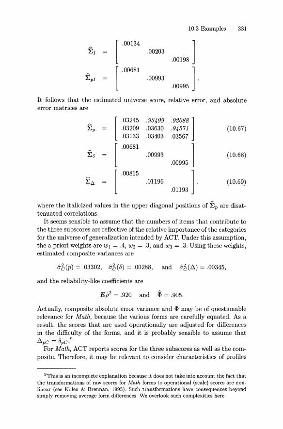
10.3 Examples 331

[.00134

.00198 ]}SI .00203

~pI[ .00681

.00993.00995 ] .

It follows that the esti mated univer se score, relative error , and abso lut eerror matrices are

[.03245 .93499 .92088 ]

~p .03209 .03630 .94571 (10.67).03133 .03403 .03567

[.00681

.00995 ]:Es .00993 (10.68)

:Eil[ .00815

.01196.01193 ] ,

(10.69)

where the italicized values in the upper diagonal posit ions of }Sp are dis at­tenuat ed correlat ions .

It seems sensi ble to assume t hat the numbers of it ems that contribute tothe three su bscores are reflective of the relative importan ce of the categoriesfor the univer se of generalizat ion intended by ACT. Under this assumpt ion ,the apriori weights are W l = .4, W2 = .3, and W3 = .3. Using these weights ,est imated compos ite varian ces are

a-b(p) = .03302, a-b(8) = .00288, and a-b(ß) = .00345,

and the reliability-like coefficients are

E ß2 = .920 and q> = .905.

ActuaIly, composite absolute error vari an ce and q> may be of questionablerelevan ce for Math, because t he various form s are carefully equated . As aresult , the scores that are used ope rat ionally are adjusted for differencesin the difficulty of the form s, and it is probably sensible to assume thatßpc = 8pc .9

For Math, ACT rep orts scores for the three subscores as weIl as the com­posite . Therefore, it may be relevant to consider characterist ics of profiles

9This is an incomplete explanation because it doesnot take into account the fact thatthe transformations of raw scores for Math forms to operational (scale) scores are non­linear (see Kolen & Brennan, 1995) . Such transformat ions have consequences beyondsimply removing average form differences. We overlook such complexit ies here.

332 10. Multivariate D Studies

of subscores for Math. Although subscores for individuals are not available,we can use the variance formulas in Section 10.2.5 to characterize the pro­file for a typical examinee. For example, using Equation 10.57 the expectedvariance of the profile of universe scores is

V(ILp ) = (.03481 - .03326) + .00616 = .0077,

and using Equation 10.57 the expected variance of the profile of observedscores is

V(Xp ) = (.04370 - .03622) + .00616 = .0136,

where .00616 is the average (over forms) of the variance of the three meanscores.!" It follows that, for a typical person, the proportion of the variancein observed scores explained by universe scores isll

9 = .0077 ~ .57..0136

In this sense, we might say that universe-score profiles are a little over50% flatter than observed-score profiles. Another interpretation is that ageneralizability coefficient for a typical person is approximately .57, in thesense discussed in Section 10.2.5.

Importance of Table of Specifications

The disattenuated correlations in Ep in Equation 10.67 are all quite high,which certainly suggests that the constructs underlying the three subscoresare highly correlated. This does not mean, however, that adherence to thetable of specifications is of little importance. One perspective on this issueis to consider the consequences of assigning all items to one of the threecategories.

For example, the mean-square relative error associated with assigningall 60 items to the first category is obtained using Equation 10.37 withal = 1, a2 = 0, and a3 = 0, and with nil = 60, ni2 = 0, and ni3 = O.This gives MSEc(8) = .00418. Assigning all items to the second cate­gory gives MSEc(8) = .00442, and assigning them to the third categorygives MSEc(8) = .00479. These values are about 50% larger than compos­ite relative error variance [o-b(8) = .00288], which clearly illustrates thatadherence to the table of specifications has an impact on measurement pre­cision. Of course, minor deviations from the 24/18/18 specifications wouldmake much less difference.

lOIn computing both V(JLp) and V(Xp) , we have dropped the (np - l)/np factor. Itis unimportant with over 3000 examinees per form.

llThis result is for illustrative purposes only ; it is based on raw scores, not the scalescores actually reported for Math .

10.3 Examples 333

More about Standard Errors

Because data for multiple forms are available for Math, standard errors ofvariance and covariance components for the universe of admissible obser­vations are easily estimated without making any normality assumptions,as discussed previously. However, it is instructive to consider what the es­timated standard errors might be under normality assumptions.

For example, using Equation 9.55, the estimated standard error of 0-12(p)for any given form is

Sr(p) S~(p) + [S12(p)J2(np - 1) + 2

whereS;(p) = o-;(p) + o-;(pi) /niV '

Using this formula with data for the first form in Table 10.4 gives

(.03947)(.04636) + (.03249)2 .3000 = .001,

where 3000 is an approximate sampie size.12

The reader ean verify that the estimated standard errors of 0-12(p) for allnine forms are about the same size, namely, .001. This is about three timessmaller than the estimate based on direct computation without normalityassumptions, namely, .003, as provided in Table 10.4. A eomparable resultholds for the other estimated covariance components. Also, the standarderrors of the estimated variance components are too small under normal­ity assumptions. Clearly, for this example, the normality-based formulaslead to underestimates of estimated standard errors . This result may beinfluenced by the fact that the underlying data are diehotomous . Also,the very large sample size for persons pretty much guarantees that thenormality-based estimates will be small for estimated varianee and covari­anee eomponents involving p .

Estimated variance and eovarianee eomponents are not only fallible­they are also correlated. For Math the varianees and eovarianees (overforms) of the o-~ (p) and the o-vv' (p) are provided in the middle of Table 10.4.The square roots of the variances are the standard errors. The upper diago­nal elements are correlations. It is evident that some of these estimates aresubstantially correlated. The availability of multiple forms makes it possi­ble to estimate the variances and eovariances of the o-~ (p) and the o-vv' (p)relatively easily, and without making normality assumptions.

D study estimated composite variances such as o-b(p), o-b(8) , and o-b(.~)

are subject to sampling variability, too . When multiple forms are available ,

12The actual sampie size for the first form and all the other forms is slightly largerthan 3000, but that is immaterial here.

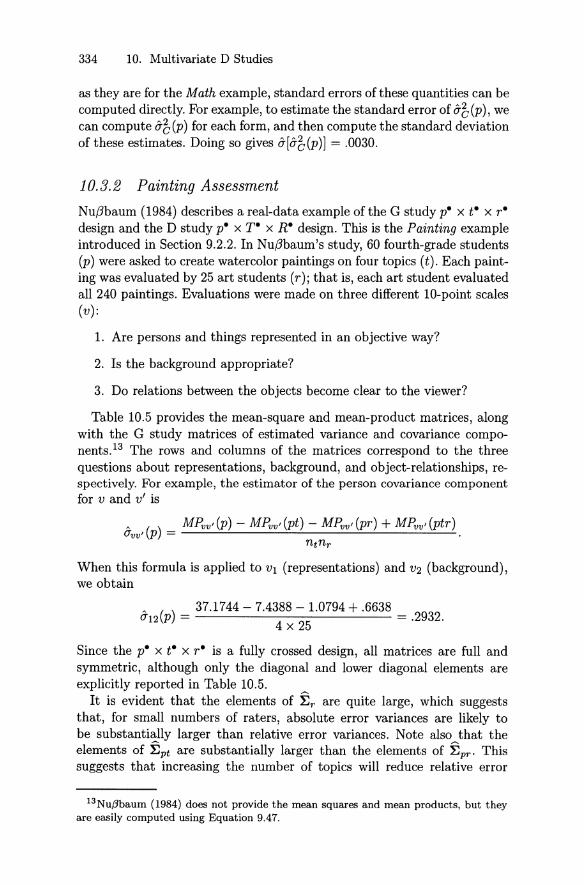
334 10. Multivariate D Studies

as they are for the Math example, standard errors ofthese quantities can becomputed directly. For example, to estimate the standard error of o-b(p), wecan compute o-b(p) for each form, and then compute the standard deviationof these estimates. Doing so gives o-[&b(p)] = .0030.

10.3.2 Painting Assessment

Nußbaum (1984) describes a real-data example of the G study p. x t· x r·design and the D study p. x T· x R· design. This is the Painting exampleintroduced in Section 9.2.2. In Nußbaum's study, 60 fourth-grade students(p) were asked to create watercolor paintings on four topies (t). Each paint­ing was evaluated by 25 art students (r ); that is, each art student evaluatedall 240 paintings. Evaluations were made on three different lO-point scales(v):

1. Are persons and things represented in an objective way?

2. Is the background appropriate?

3. Do relations between the objects become clear to the viewer?

Table 10.5 provides the mean-square and mean-product matriees, alongwith the G study matrices of estimated variance and covariance compo­nents .P The rows and columns of the matriees correspond to the threequestions about representations, background, and object-relationships, re­spectively. For example, the estimator of the person covariance componentfor v and v' is

o-vv,(p) = MPvv'(p) - MPvv,(pt) - MPvv,(pr) + MPvv,(ptr) .ntnr

When this formula is applied to VI (representations) and V2 (background) ,we obtain

A () 37.1744 - 7.4388 - 1.0794+ .66380'12 P = 4 x 25 = .2932.

Since the p. x t· x r" is a fully crossed design, all matrices are full andsymmetrie, although only the diagonal and lower diagonal elements areexplicitly reported in Table 10.5.

It is evident that the elements of ~r are quite large, whieh suggeststhat, for small numbers of raters, absolute error variances are likely tobe substantially larger than relative error variances. Note also that theelements of ~Pt are substantially larger than the elements of ~pr' Thissuggests that increasing the number of topies will reduce relative error

13Nußbaum (1984) does not provide the mean squares and mean products, but theyare easily computed using Equation 9.47.

10.3 Examples 335

TABLE 10.5. G Study for Painting Example

Mp~ [52.9630

52.4574]

[ .4156

.3897 ]37.1744 43.2336 :Ep = .2932 .315349.0604 42.4304 .3908 .3295

[ 79.5866

55.9722]

[ 04U

.0252 ]M t = -37.6932 26.3060 :Et = -.0314 .0053

42.9452 -21.4924 .0196 -.0217

[ 332.6465

384.1964]

[ 1.3568

1.5703 ]M r = 268.7274 288.0886 :Er = 1.1070 1.1601

321.8674 304.6384 1.3196 1.2549

[ 10.8626

13.0002]

[ .3805

.4534 ]M pt = 7.4388 10.9400 :Ept = .2710 .3782

9.5672 8.9156 .3518 .3264

Mp" ~ [1.8905

2.1492]E~~ [

.1351

1218 ]1.0794 2.2486 .1039 .19091.1852 1.3204 .1033 .1412

M," ~ [6.4741

6.8372]E,"~ [

.0854

.0862 ]2.6318 8.9010 .0328 .12364.7502 2.8976 .0663 .0357

Mp'" ~ [1.3501

1.6652]

[ 1.3501

1.6652 ].6638 1.4850 :Eptr = .6638 1.4850.7722 .7556 .7722 .7556

Note. All matriees are symmetrie. SampIe sizes are: np = 60 students, nt = 4 topics,a n d n r = 25 rat ers.

variance faster than a corresponding increase in the number of raters. Thesesomewhat abstract statements, of course, should be confirmed by examiningspecific D study results.

Raters Random

The top half of Table 10.6 reports D study result s for the D st udy randomeffects p. x T· x R· design based on two raters and two topics, as wellas two raters and four topics . For both pairs of D study sample sizes, esti­mat ed universe-score, relative-erra r, and absolute-errar varian ce-covariancematrices are reported. For this random effects mult ivariate design, t he es­timated universe score matrix is simply f:p . The estimated relat ive-errormat rix is

336 10. Multivariate D Studies

TABLE 10.6. Same D Study Results for Paint ing Example

Raters Random with n~ = 2

n~ = 2 n~ = 4

[.4156 .810 .971 ] [

.4156 .810 .971 ]Er .2932 .3153 .940 .2932 .3153 .940

.3908 .3295 .3897 .3908 .3295 .3897

[ .5953 .566650 ] [ .3314 .574 .663 ]~

Eo .3534 .6558 .622 .2027 .3756 .651.4206 .4227 7039 .2361 .2467 .3824

[ 1.3163 .696 .782 ] [ 1.0311 .751 .823 ]E~ .8994 1.2694 .754 .7524 .9725 .814

1.1068 1.0482 1.5232 .9091 .8731 1.1846

Composite Defined Using Weights of Wl = .50, W2 = .33, and W3 = .17

a-b(T) .349 .349a-b(8) .476 .270

a-b(ß) 1.113 .898E ß2 .423 .564

~ .239 .280

One Fixed Rater

n~ = 2 n~ = 4

[ .5507 .752 .931 ] [.5507 .752 931 ]

Er .3971 .5062 .925 .3971 .5062 .925.4941 .4707 .5115 .4941 .4707 .5115

[.8653 .521 587 ] [ .4327 .521 587 ]

Eo .4674 .9316 .545 .2337 .4658 .545.5620 .5410 1.0593 .2810 .2705 .5297

[.9292 ·487 594 ] [ .4646 ·487

594

]E~ .4681 .9961 .520 .2341 .4980 .520

.6050 .5480 1.1150 .3025 .2740 .5575

Composite Defined Using Weights of Wl = .50, W2 = .33, and W 3 = .17

.475

.659

.692

.419

.407

.475

.329

.346

.591

.579

Note . Italicized values in upper off-diagonal positions are correlations.

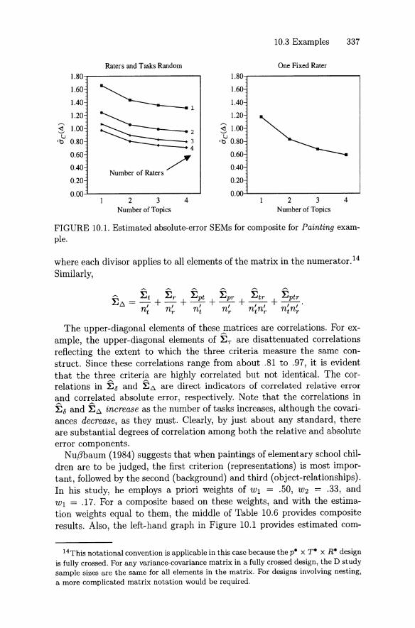
10.3 Examples 337

Raters andTasks Random One Fixed Rater1.80 1.80

1.60

~11.60

1.40 1.40

1.20

~~;1.20

~

1.00 ~ 1.00<]

'G. ~ 0.80' b 0.80

0.60 -: 0.60

0.40 0.40Number of Raters

0.20 0.20

0.00 0.002 3 4 2 3 4

Numberof Topics Number ofTo pics

FIGDRE 10.1. Estimated absolute-error SEMs for composite for Painting exam-ple,

where each divisor applies to all elements of th e matrix in th e numerator. 14

Similarly,

The upper-diagonal elements of these matrices are correlat ions. For ex­ample, t he upper-diagonal elements of Er are disattenuated correlationsreflecti ng the extent to which th e three criteria measure th e same con­struct . Since these correlat ions range from about .81 to .97, it is evidentthat th e three crite ria are highly correlated but not ident ical. The cor­relat ions in ~o and ~t:. are direct indicators of correlated relative errorand correlated absolute error, respect ively. Note that the correlat ions inEo and Et:. increase as the number of tasks increases, although the covari­ances decrease, as they must. Clearly, by just about any standard, t hereare substant ial degrees of correlat ion among both th e relative and absoluteerror components.

Nuß baum (1984) suggests that when paintings of elementary school chil­dren are to be judged, the first crite rion (representat ions) is most impor­tant , followed by the second (background) and third (object-relationships).In his st udy, he employs a priori weights of W 1 = .50, W2 = .33, andW1 = .17. For a composite based on th ese weights , and with the estima­t ion weights equal to them, the middle of Table 10.6 provides compositeresults. Also, t he left-hand graph in Figure 10.1 provides esti mated com-

14This not at ional convention is applicable in t his case because t he p. x T · x R· designis fully crosse d. For any var iance-covariance matrix in a fully crossed design, t he D studysampie sizes are t he same for all elements in th e matrix. For designs involving nest ing,a more complicated matrix notation would be required.

338 10. Multivariate D Studies

posite absolute-error SEMs for numbers of raters and topics ranging fromone to four. If an investigator wanted 68% of the students to have universescores within one absolute-error SEM of their observed scores, Figure 10.1suggests that it would be appropriate to use two raters and three topics.

One Fixed Rater

Nußbaum (1984, p. 227) states,

A teacher may have good reason not to generalize over judges.He or she may, for example, regard his or her own statement asthe only valid one because other teachers have no knowledge ofthe conditions under which the pictures were painted.

Nußbaum uses this logic in support of performing a multivariate D studyanalysis for a single fixed rater, in the sense discussed in Section 10.2.7.That is, his D study analysis collapses over the levels of the rater facet. Or ,stated differently, the rater facet is treated as fixed in the univariate sensewith n~ = l.

The bottom half of Table 10.6 reports results for the p. x T· x R·D study design with a single fixed rater, for two and four topics . For thisdesign, the estimated universe score matrix is

~T = ~p + ~PTl

the estimated relative-error matrix is

and the estimated absolute-error matrix is

~ _ ~t ~Pt ~tr ~Ptr.6.- I + I + I + I'nt n t n t n t

The bottom of Table 10.6 provides composite results using the aprioriweights of Wl = .50, W2 = .33, and Wl = .17. Also, the right-hand graph inFigure 10.1 provides estimated composite absolute-error SEMs for one tofour topics. As in univariate theory, fixing raters leads to smaller compositeerror variances and SEMs, and larger coefficients.

Nußbaum's (1984) one-fixed-rater D study analysis is probably not ideal.The likely ideal would be to conduct separate D study p. x T· analyses foreach specific judge of interest. Alternatively, if the judges of interest werethe same 25 judges used in the G study, then a multivariate p. x T· analy­sis with 25 x 3 = 75 levels of v could be employed. Neither of these idealizedalternatives is likely to be viable in most circumstances, and Nußbaum's(1984) one-fixed-rater D study analysis is a reasonable alternat ive for prac­tical use.

10.3 Examples 339

10.3.3 Listening and Writing Assessment

Brennan et al. (1995) describe a Listening and Writing assessment thatprovides an example of the G study p. x t· x t" design, and the D studyp. x T· x RO and p. x TO x RO designs . This is the LW example intro­duced in Section 9.2.2. Each of three preliminary forms (402, 404, 406) ofthe Listening and Writing tests was administered to one of three groups of50 examinees. Each examinee (p) listened to 12 tape-recorded messages (t) .For each form, the messages were different . Examinees were told to takenotes while each message was played. At the conclusion of each message,examinees were told to use their notes to construct a written message. Thewritten messages were scored by trained raters on a five-point holistic scalefor both listening skills (L) and writing skills (W). The listening score re­fiected the accuracy and completeness of the information provided in thewritten messages . The writing score refiected other aspects of the "qual­ity" of the writing. For each form there were two distinct sets of raters (r) .Three raters evaluated the written messages for listening, and a differentthree raters evaluated the messages for writing. The groups of listening andwriting raters were different for each form.

This is a relatively rare example of a true G study in the sense that theprimary purpose of gathering the data was to obtain empirical evidenceto inform judgments about the design characteristics of measurement pro­cedure that would be used operationally, Table 10.7 provides the G studyvariance and covariance matrices for each of the forms, as well as the aver­ages over forms. For each matrix, the first row and column is for Listeningand the second is for Writing.

Also provided in Table 10.7 are the estimated standard errors of theaverages of the estimated variance and covariance components. These areempirical standard errors; that is, they are the standard deviations of theelements divided by the square root of three. As such , they are not basedon any normality assumptions. In general, it is clear that the estimatedstandard errors are small relative to the estimated variance and covariancecomponents themselves.

In the remainder of our discussion of the LW example, we focus on theaverage estimates for two reasons : they are more stable than the individualform estimates, and the intended inferences to be drawn are for a "general"form (i.e., a randomly parallel form) as opposed to any specific form.

It is evident that &r (p) and &rv (p) are large relative to the other esti­mated variance components, which suggests that examinees differ consid­erably with respect to their levels of proficiency in listening and writing.Furthermore, since &rv(p) = .691 is much larger than &r(p) = .324, exami­nees appear to be much more variable in writing proficiency than listeningproficiency, as these constructs are represented in this measurement proce­dure.

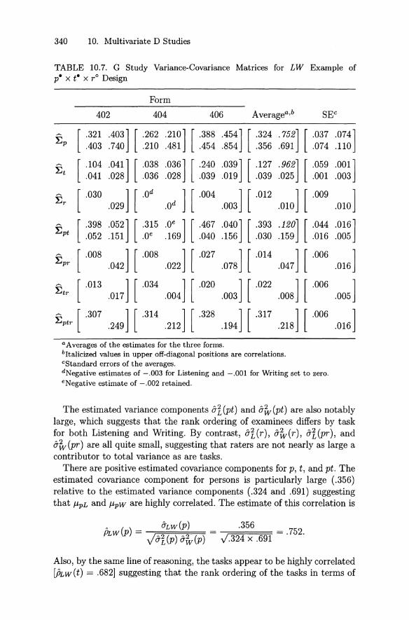
340 10. Multivariate D Studies

TABLE 10.7. G Study Variance-Covariance Matrices for LW Example ofp. x t· x TO Design

Form

402 404 406 Average'v"

.074]

.110

.001]

.003

.010]

.016]

.005

.016]

.005]

.016]

.454] [ .324

.854 .356

.039] [ .127

.019 .039

] [.012

.003

.040] [ .393

.156 .030

] [.014

.078

.Od ] [ .004

.210] [ .388

.481 .454

.036] [ .240

.028 .039

.o- ] [ .467

.169 .040

] [.027

.022

.403] [ .262

.740 .210

.041] [ .038

.028 .036

.052] [ .315

.151 .o-

] [.008

.042

.029] [ .Od

.752] [ .037

.691 .074

.962] [ .059

.025 .001

] [.009

.010

.120][ .044

.159 .016

] [.006

.047

] [.034 ] [ .020 ] [ .022 ] [ .006

.017 .004 .003 .008

] [.314 ] [ .328 ] [ .317 ] [ .006

.249 .212 .194 .218

[.321.403

~ [ .104:Et .041

[.030

:Er

~ [.398:Ept .052

[.008

:Epr

~ [ .013:Et r

~ [ .307LJptr

a Averages of the estimates for the three forms .bltalicized values in upper off-diagonal positions are correlations.CStandard errors of the averages,dNegative estimates of - .003 for Listening and - .001 for Writing set to zero .eNegative estimate of - .002 retained.

The estimated variance components iTi(pt) and iTrv(pt) are also notablylarge, which suggests that the rank ordering of examinees differs by taskfor both Listening and Writing. By contrast, iTJ,(r), iTrv(r), iTi(pr), andiTrv (pr) are all quite smalI, suggesting that raters are not nearly as large acontributor to total variance as are tasks .

There are positive estimated covariance components for p, t, and pt. Theestimated covariance component for persons is particularly large (.356)relative to the estimated variance components (.324 and .691) suggestingthat f.J,pL and f.J,pw are highly correlated. The estimate of this correlation is

.356 = .752.} .324 x .691

Also, by the same line of reasoning, the tasks appear to be highly correlated[PLW(t) = .682] suggesting that the rank ordering of the tasks in terms of

10.3 Examples 341

difficulty is quite similar for Listening and Writing . By contrast, the ptinteraction effects are only slightly correlated [PLW(pt) = .120].

Brennan et al. (1995) report a number of D study results for one, two,and three raters , but they suggest that cost factors will likely precludeusing more than two raters operationally. For this reason, here we restrietconsideration to two raters. Table 10.8 provides D study results for twodifferent design structures (p. x T· x RO and p. x TO x RO), two samplesizes for tasks (6 and 12), and two composites-an equally weighted averageof the two scores (WL = .5 and Ww = .5) and difference scores (WL = 1and Ww = -1).

The top of Table 10.8 provides D study estimated variance-covariancematrices followed by the matrix Clf estimated absolute-error variance andcovariance components. In both ~p and ~6 italicized values are correla­tions . The estimated correlation between universe scores for Listening andWriting is .752. For the p. x T· x RO design, the L\-type errors have anestimated correlation of .114. These errors are necessarily uncorrelated forthe p. x TO x RO design.

The p. x T· x RO design has the same design structure as that in theG study. It assurnes that the same tasks would be used to obtain scoreson Listening and Writing. By contrast, for the p. x TO x RO design, thetasks used to obtain a Listening score would be different from those usedto obtain a Writing score. For both designs, of course, the use of moretasks reduces composite absolute error variance and increases indices ofdependability, for both composites .

A principal difference between the p. x T· x RO and p. x TO x RO de­signs is that the p. x T· x RO design has an estimated absolute error covari­ance of (J'Lw(L\) = .011 for 6 tasks and (J'Lw(L\) = .006 for 12 tasks, whereasthere is no absolute error covariance component for the p. x TO x RO de­sign. The role of (1"Lw(L\) in the two designs has very different consequencesfor the two composites. Specifically,

• for the composite based on averaging the two scores, the positive co­variance component for the p. x T· x RO design causes a-b(L\) to belarqer for the p. x T· x RO design than for the p. x TO x RO design;whereas,

• for the "difference" composite , the positive covariance componentfor the p. x T· x RO design causes a-b (L\) to be smaller for thep. x T· x RO design than for the p. x T Ox RO design.

All other things being equal , this suggests that the p. x T· x RO design ispreferable when the composite is a difference score, but the p. x TO x ROdesign is preferable when the composite is an average score-providedO'b(L\) is positive.

Positively correlated error decreases O'b(L\) when the composite is a dif­ference score, because O'LW (L\) has a negative contribution to absolute error

342 10. Mult ivariate D Studi es

TABLE 10.8. D Study Variance-Covariance Matrices and Composite Results forLW Example with Two Raters

p. x T· x Ra Design p. x Ta X Ra Design

n~ = 6 n~ = 12 n~ = 6 n~ = 12

~p[ .324 .752] [ .324 .752] [ .324 .752] [ .324 .752]

.356 .691 .356 .691 .356 .691 .356 .691

~T[ .021 .006] [ .011 .003] [ .021

.004][ .011

.002].006 .004 .003 .002

~R[ .006

.005][ .006

.005][ .006

.005][ .006

.005]

~pT[ .066 .005] [ .033 .003] [ .066

.026][ .033

.013 ].005 .026 .003 .013

~pR[ .007

.024][ .007

.024][ .007

.024][ .007

.024]

~TR [ .002.001]

[ .001.000]

[ .002.001]

[ .001.000]

~pTR[ .026

.018][ .013

.009][ .026

.018][ .013

.009]

~6[ .128 .114] [ .070 .093] [ .128 ] [ .070

.053].011 .078 .006 .053 .078

Composite Defined Using Weights of WL = .5 and Ww = .5

o-ß(p) .432 .432 .432 .432o-ß(~l .057 .034 .051 .031

<I> .883 .928 .894 .933

Composite Defined Using Weights of WL = 1 and Ww = - 1

o-b(p) .304 .304 .304 .304o-ß(~) .183 .112 .206 .124

~ .624 .730 .596 .711Not e. Italicized values in upper off-diagonal positions are correlations.

10.4 Exercises 343

variance for difference scores:

By cont rast , for the "average" composite,

10.4 Exercises

10.1* For the Rajaratnam et al. (1965) synthetic data example consideredin Section 9.1 (see, especially, Table 9.1 on page 270), provide ETl

E.s , ~~ for the total score metric . For this metric, specify the wweights and use th em to obt ain o-b(r), o-b(6), and o-b(ß). Verifythat Eß2 and ~ are unchanged by this change in metric.

10.2* For the Rajaratnam et al. (1965) synthetic dat a example in Sec­tion 9.1, if the a priori weights were all one-third, what would bethe sample sizes th at minimize absolute error variance under theconst raint th at n~+ = 107

10.3 For the Rajaratnam et al. (1965) synthet ic dat a example in Sec­tion 9.1, what is MSEc(ß) if all eight items were assigned to thesecond category, but the w weights stay unchanged (i.e., .25, .50,and .25, respectively)7

10.4 Consider a multivariate p. x r design with two levels of a fixedfacet , and suppose that o-r(I) = o-~(I) , o-r(pI) = o-~(p1) , and bothest imated D study covariance components are positive. Under whatcircumstances is P12(8) > Pt2(ß)7

10.5* For the synt het ic dat a example in Section 10.1.6, what is o-b(ß) forth e D study r :p. design assuming n~ = 8, W1 = .75, and W2 = .257

10.6* For the example in Section 10.1.6, what is Ep2 for the D studyp. x 1° design assuming n~ = 8, W 1 = .75, and W2 = .257 Providea verbal description of the p. x 1° design for the accuracy/speedmeasurement procedure. If items were administered by computer,is this a likely design for this hypothetical exarnple?

10.7 For the synthet ic data example in Section 10.1.6 (see, also, Table 9.3on page 292), suppose the investigator considered accuracy andspeed to be equally important in characte rizing the universe ofgeneralization. Further suppose she had to do scoring by hand ,and her scoring resources were limited, so much so th at she couldafford to score only two items for each student . However , she can

344 10. Multivariate D Studies

administer as many items as she wants, and she can get a measure ofspeed for each student on each item. She decides that students willtake different items, but they will all take the same number of items.It is important, she decides, that the SEM for the composite be nolarger than 2/3. What number of items should be administered toeach student?

10.8* For the synthetic data example discussed in Section 10.2.3, what are8'0(.0'1) and 8'0(<5I) for the p. x J. design with n~ = 8, Wl = .75,and W2 = .25?

10.9 For the synthetic data example in Section 9.1 (raw data in Table 9.1on page 270) with apriori weights proportional to sample size, whatis the conditional absolute standard error of measurement for thefirst person, using the mean-score metric?

10.10 Derive Equation 10.54 based on the classical test theory model withuncorrelated error and assuming that (jEx = oe; = (JE .

10.11 Section 10.2.3 provided conditional SEMs for the first person in thesynthetic data in Table 9.3 on page 292. What is the probabilitythat 68% confidence intervals for this person will overlap if the truedifference in this person's universe scores is J1.n - J1.12 = .5?

10.12* Suppose a test called Science Assessment consists of two separatelytimed parts. Part 1 contains 24 dichotomously scored items. Part2 contains two open-ended items with responses coded 0 to 4. Thetechnical manual for Science Assessment provides the followinginformation,

MeanStandard DeviationCoefficient alpha

Part 116.003.64

.70

Part 24.001.82

.50

where the means and standard deviations are for total scores. Thecorrelation between total scores on the two parts is .40.

(a) Provide ~p and ~Pi for both the mean-score metric and thetotal-score metric .

(b) Provide ~'T and ~ö for both the mean-score metric and thetotal-score metric .

(c) Procedures in classical test theory for estimating the reliabilityof a battery composite (see Feldt & Brennan, 1989, p. 117)yield a coefficientof .742. Show that this value can be obtainedeasily from the total-score ~'T and ~ö matrices .

10.4 Exercises 345

~ ~

(d) Using the mean-score :Er and :Eö matrices, what are the wweights that are required to give the classical reliability coef­ficient of .742 in (c)?

(e) Provide at least one advantage and one disadvantage of theclassical test theory procedure in (c) compared to the proce­dure in (d) .

(f) What is the contribution of Part 1 to composite universe (ortrue) score variance? Show that the answer is the same forboth the mean-score and total-score metrics .

(g) The technical manual for Science Assessment states that, "Co­efficient alpha for Part 2 is based on a single rating of eachexaminee 's response to each open-ended item." Discuss the ap­propriateness of Coefficient alpha under these circumstances.

10.13 For Nußbaum's (1984) Painting example, Table 10.6 reports that0'12(0) = .2027. Under normality assumptions, what is the esti­mated standard error of this covariance component?

10.14 Consider the G study variance-covariance matrices for the LW ex­ample in Table 10.7. Provide an estimate of the standard error ofO'LW(p) if Form 402 were the only form available, Discuss this esti­mate relative to the standard error of .074 reported in Table 10.7.

10.15* Recall Exercise 9.9 based on the study by Miller and Kane (2001).Suppose categories are considered fixed, and the D study samplesizes are the same as those in the G study. Provide ~r, ~ö , and~A ' For the difference-score composite, determine O'b(T), O'b(o) ,and O'b (.6.) . If Xl = .2578 and X 2 = .7955 in the proportion­correct metric, estimate the error-tolerance ratio (see Section 2.5.1)for absolute interpretations of difference scores; that is, estimate

E/T=

11Multivariate Unbalanced Designs

The power and flexibility of multivariate generalizability are purchasedat the price of complex conceptual and statistical issues that become evenmore challenging in unbalanced situations. Recall that a covariance compo­nents design is called unbalanced in this book if either of the correspondingvariance components designs is unbalanced. Many real-data applications ofmultivariate generalizability theory involve unbalanced situations. 1

For unbalanced multivariate designs, perhaps the most challenging sta­tistical issue is the estimation of covariance components. That is the subjectof Section 11.1. D study issues are considered subsequently in Section 11.2in the context of several real-data examples . Most of the D study formulasand theoretical results for balanced designs discussed in Chapter 10 alsoapply in unbalanced situations.

11.1 Estimating G Study Covariance Components

For balanced covariance components designs, the expected-mean-productequations are relatively simple, and it is easy to use them to estimate the co­variance components. For unbalanced covariance components designs, how­ever, complexities arise. The fundamental theoretical problem is that there

1 As noted in Chapter 8, randomly discarding data to achieve a balanced univariatedesign is often problematic. In most cases, there is good reason to beli eve that this adhoc strategy is likely to be even more problematic when applied to multivariate designs,

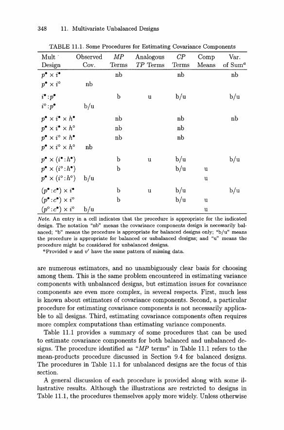
348 11. Multivariate Unbalanced Designs

TABLE 11.1. Some Procedures for Estimating Covariance Components

Mult :Design

p. x i· x h·p. x i· x hO

p. x iOx h·p. x iO x hO

ObservedCov.

nb

b/u

nb

MPTerms

nb

b

nb

nb

nb

AnalogousTP Terms

u

CPTerms

nb

b/u

nb

nb

nb

CompMeans

Var.of Sum"

nb

b/u

nb

p·xW:h·)

p·xW :h·)p·xW:hO) b/u

(p· :c·) x i·(p. .c") x iO

(po :c·) x iO b/u

b

b

b

b

u

u

b/ub/u

b/ub/u

u

u

u

u

b/u

b/u

Note . An entry in a cell indicates that the procedure is appropriate for the indicateddesign. The notation "nb" means the covariance components design is necessarily bal­anced; "b" means the procedure is appropriate for balanced designs only ; "b/u" meansthe procedure is appropriat e for balanced or unbalanced designs ; and "u" means theprocedure might be considered for unbalanced designs.

aProvided v and o' have the same pattern of missing data.

are numerous estimators, and no unambiguously clear basis for choosingamong them. This is the same problem encountered in estimating variancecomponents with unbalanced designs, but estimation issues for covariancecomponents are even more complex, in several respects. First, much lessis known about estimators of covariance components. Second, a particularprocedure for estimating covariance components is not necessarily applica­ble to all designs. Third, estimating covariance components often requiresmore complex computations than estimating variance components.

Table 11.1 provides a summary of some procedures that can be usedto estimate covariance components for both balanced and unbalanced de­signs. The procedure identified as "MP terms" in Table 11.1 refers to themean-products procedure discussed in Section 9.4 for balanced designs.The procedures in Table 11.1 for unbalanced designs are the focus of thissection .

A general discussion of each procedure is provided along with some il­lustrative results . Although the illustrations are restricted to designs inTable 11.1, the procedures themselves apply more widely. Unless otherwise

11.1 Estimating G Study Covariance Components 349

noted, the term "unbalanced" is to be understood as unbalanced with re­spect to nesting only-not missing data. Some of the procedures discussedare applicable to designs that involve missing data, but this topic is nottreated explicitly until Section 11.1.6.

Estimating covariance components for unbalanced designs is one of themost complicated statistical issues covered in this book. Some readers maywish to skim this section initially and return to it after studying the exam­ples in Section 11.2.

11.1.1 Observed Covariance

When the only linked facet is that for the objects of measurement [e.g.,p in the p. x W: hO) design], the covariance of the observed mean scoresfor that facet is an unbiased estimator of the covariance component. Forunbalanced designs, the observed mean is defined here as the simple averageover all levels of all facets. So, for example, for the multivariate unbalancedp. x W: hO) design

(11.1)

a similar expression applies for X pv', and the observed covariance is givenby Equation 9.7. We call the expression for X pv in Equation 11.1 a simplemean to distinguish it from the mean (over levels of h) of the mean (overlevels of i). We consider covariance components based on such compoundmeans later. Unless otherwise noted, all references to mean scores implysimple means. Of course, simple means and compound means are equivalentfor balanced designs .

11.1.2 Analogous TP Terms

Recall from Section 7.1.1 that analogous T terms can be used to estimatevariance components when the variance components design is unbalanced.Similarly, for some unbalanced covariance components designs, analogousTP terms can be used to estimate covariance components. Specifically,analogous TP terms can be used to estimate covariance components forunbalanced multivariate designs in which all levels of all facets are linked,which implies that the variance components designs and the covariancecomponents designs have the same structure. We say that such designs are"full"; that is, each facet has a superscript filled circle in the representationof the multivariate design .

The definition and use of analogous TP terms parallels the definitionand use of analogous T terms, as discussed in Section 7.1.1. Specifically,analogous TP terms are defined as

TPvv'(O:) = Ln"X"vX"v1,

Ci

(11.2)

350 11. Multivariate Unbalanced Designs

where na is the total number of observations for a given level of o, and themean scores (X av and X av') are sums of observations divided by the totalnumber of observations summed (e.g., Equation 11.1).

The coefficient of /-Lv/-Lv' in the expected value of every TP term is simply

(11.3)

where n+ is the total number of observations for v (or v') in the design.PThe coefficient of O"vv' (o) in the expected value of the TP term for ß is

(11.4)

where

/ is the set of an indices in a that are not in ß (if ß = /-L , then/ = o};

nß"! is the total number of observations in the variance componentsdesign that is associated with a given combination of levels of ßand /; and

nß is the total number of observations for a given level of ß (notethat nß = L,,! nß"!) '

One useful special case of Equation 11.4 is-2

k[o-vv,(a) ,ETPvv'(/-Lv/-Lv')] = :L na, (11.5)

o n+

where na is the total number of observations for a given level of o. Notealso that

(11.6)

andk[O"vv,(a),ETPvv'(w)] = n+, (11.7)

where w is the effect associated with an the indices in the covariance com­ponents design.

Consider, for example, the unbalanced i· :p. design in which ni :p is nota constant for an p. The analogous TP terms are

TPvv,(i:p)

L ni:pXpv X pv'p

L L XpivXpiv'p

n+XvXv"

(11.8)

2For full multivariate designs, the total number of observations is the same for bothv and v' .

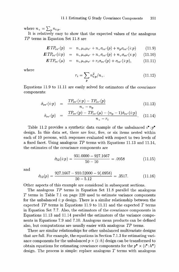
11.1 Estimating G Study Covariance Components 351

where n., = L pni:p 'It is relatively easy to show that the expected values of the analogous

TP terms in Equation Set 11.8 are

where

E TPvv'(p)

ETPvv,(i:p)

ETPvv'(/-l)

n+/-lv/-lv' + n+O"vv'(p) + npO"vv,(i :p)

n+/-lv/-lv' + n+O"vv'(p) + n+O"vv ,( i :p)

n+/-lv/-lv' + Ti O"vv' (P) + O"vv,(i :p),

(11.9)

(11.10)

(11.11)

(11.12)

Equations 11.9 to 11.11 are easily solved for est imators of the covariancecomponents:

o-vv'(p)

n+ - np

TPvv'(p) - TPvv'(/-l) - (np - 1)o-vv,( i:p)

(11.13)

(11.14)

Table 11.2 provides a synthet ic data example of the unbalanced i·: p.design. In this data set , there are four, five, or six items nested withineach of 10 persons , with responses evaluated with respect to two levels ofa fixed facet . Using analogous TP terms with Equations 11.13 and 11.14,the est imates of the covariance components are

and

~ ( ) 931.0000 - 927.16670"1 2 i :p = = .0958

50 -10

~ ( ) _ 927.1667 - 910.52000 - 9( .0958) _0"12 P - 50 _ 5.12 - .3517.

(11.15)

(11.16)

Other aspects of this example are considered in subsequent sections .The analogous TP terms in Equation Set 11.8 parallel the analogous

T terms in Table 7.1 on page 220 used to est imate variance componentsfor the unbalanced i :p design. There is a similar relationship between theexpected TP terms in Equations 11.9 to 11.11 and the expected T termsin Equation Set 7.7. Also, the est imators of th e covariance components inEquations 11.13 and 11.14 parallel the est imators of the variance compo­nents in Equations 7.9 and 7.10. Analogous mean products can be definedalso, but computat ions are usually easier with analogous TP terms.

There are similar relationships for other unbalanced multivariate designsthat are full. For example, the equat ions in Section 7.1.3 for estimating vari­ance components for the unbalanced p x (i :h) design can be transformed toobt ain equat ions for est imat ing covariance components for the p. x (i . :h·)design. The process is simple: replace analogous T terms with analogous

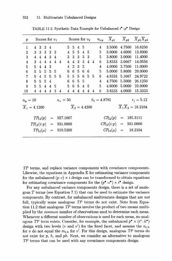
352 11. Multivariate Unbalanced Designs

TABLE 11.2. Synthetic Data Example for Unbalanced i" :p" Design

p Scores for Vi Scores for V2 ni:p X pl X p2 X plXp2

1 4 3 3 4 5 5 4 5 4 3.5000 4.7500 16.62502 3 3 3 3 3 4 5 5 4 5 5 3.0000 4.6000 13.80003 4 4 4 3 4 3 3 3 3 3 5 3.8000 3.0000 11.40004 3 4 4 4 4 4 4 4 3 3 4 4 6 3.8333 3.6667 14.05565 5 4 4 3 4 2 3 2 4 4.0000 2.7500 11.00006 5 5 5 5 5 6 6 5 6 6 5 5.0000 5.8000 29.00007 5 4 5 5 5 5 5 5 5 6 5 5 6 4.8333 5.1667 24.97228 5 5 5 4 6 6 5 5 4 4.7500 5.5000 26.12509 5 5 4 4 5 5 6 5 4 5 5 4.6000 5.0000 23.0000

10 4 4 4 4 3 4 4 4 4 4 4 4 6 3.8333 4.0000 15.3333

np = 10 n+ = 50 iii = 4.8781 Ti = 5.12

Xl = 4.1200 X 2 = 4.4200 X 1X2 = 18.2104

TP12(P) = 927.1667 C112(p) 185.3111

TP12(i:p) = 931.0000 CP12(i :p) 931.0000

TPdJ.L) 910.5200 C112(J.L) 18.2104

TP terms, and replace variance components with covariance components .Likewise, the equations in Appendix E for estimating variance componentsfor the unbalanced (p :c) x i design can be transformed to obtain equationsfor est imating covariance components for the (po:CO) x iOdesign.

For any unbalanced variance components design, t here is a set of analo­gous T terms (see Equat ion 7.1) that can be used to esti mate the variancecomponents. By contrast, for unbalanced mult ivariate designs that are no tfuII, typicaIIy some analogous TP terms do not exist . Note from Equa­t ion 11.2 that analogous TP terms involve the product of two means multi­plied by the common number of observations used to determine each mean.Whenever a different number of observations is used for each mean , no anal­ogous TP term exists. Consider, for example, the unbalanced pOx (io: hO)design with two levels (v and v' ) for the fixed facet , and assurne the ni:hfor v do not equal the m i:h for v'. For this design, analogous TP terms donot exist for p, h, and ph. Next , we consider an alternative to analogo usTP terms that can be used with any covariance components design.

11.1 Estimating G Study Covariance Components 353

11.1.3 CP Terms

Another approach for est imat ing covariance components for an unbalanceddesign involves direct use of th e sums-of-cross-products terms and their ex­pected values. These lead to a set of simultaneous linear equat ions that canbe solved for the estimated covariance components . This approach is quit egeneral in th at it can be used for any unbalanced covariance componentsdesign , but expressions for the resulting estimated covariance componentsare often complex.

A sum-of-cross-products term for a component a in a covariance compo­nents design is

if o :/= J-l

(11.17)

if a = J-l

where the mean scores in Equation 11.17 are sums of observations dividedby the total number of observations summed (e.g., Equation 11.1) . Com­paring Equations 9.45 and 11.17, it is obvious that for balanced designsTP terms and CP terms differ only by a multiplicative factor, 1r(a) . Forbalanced designs, TP terms have the advantage of being related to MPterms which, in turn, are easily used to estimate covariance components.For unbalanced designs, however, usually it is easier to work directly withCP terms (except , perhaps, when analogous TP terms exist).

The expected value of each CPvv' (a) term involves the product of themeans , J-lvJ-lv' , as well as each of the covariance components . The coefficientof the product of the means is

if o i= J-l

(11.18)

if a = u;

where L o (1) is the number of levels associated with o .The coefficient of each of the covariances included in the expected value

of the sum-of-cross-products term for ß is much more complicated. For anyparticular covariance component O"vv' (o), the coefficient is

(11.19)

where

, is the set of aH indices in a that are not in ß (if ß = J-l , th en, = o) ; note that , plus a includes all indices in the covariancecomponents design;

354 11. Multivariate Unbalanced Designs

if ß or / is the null set (i.e., no indices), the associated summationoperator disappears;

riß-y is the total number of observations in the variance componentsdesign for v that are associated with a given combination of levelsof ß and /;

mß-y is the total number of observations in the variance componentsdesign for v' that are associated with a given combination of levelsof ß and /;

riß is the total number of observations for a given level of ß forvariable v (riß = E-y riß-y); and

mß is the total number of observations for a given level of ß forvariable v' (mß = E-y mß-y)·

One useful special case of Equation 11.19 is

(11.20)

where ria: is the total number of observations for v for a given level of 0:,ma: is the total number of observations for v' for a given level of 0:, n+ isthe total number of observations in the variance components design for v,and rn, is the total number of observations in the variance componentsdesign for v' . Note also that

k[o-vv'(O:), ECPvv'(O:)] = I: (1), (11.21)

which is the number of levels associated with 0:; and letting w be the effectassociated with all indices in the covariance components design,

k[o-vv' (0:), ECPvv'(w)] = I: (1),w

(11.22)

which is the total number of levels for all the indices in the covariancecomponents design.

i· :p. Design

Consider, for example, the unbalanced i· :p. design. The three CP termsare

CPvv,(p)

CPvv,(i:p)

LXpvXpv'p

I:I: XpivXpiv'p

x,x;

(11.23)

11.1 Estimating G Study Covariance Components 355

For the eoefficient of O'vv'(p) in ECPvv'(/L), Equation 11.20 applies, whichgives

[ () ( )] '" npmp '" n;,p r,k O'vv' P , E CPvv' /L = LJ-- = LJ -2 =-,p n+m+ p n+ n.,

where ri is given by Equation 11.12. Using Equation 11.20 again, the eoef­fieient of O'vv' (i: p) in E CPvv' (/L) is

k[O'vv,(i :p),ECPvv'(/L)] = LL npimpi = LL~ =~.P i n+m+ p i n+ n.,

Note that both npi and mpi are unity beeause there is only one observationfor eaeh eombination of levels of p and i . The eoefficient of O'vv' (i: p) inECPvv'(p) is obtained using Equation 11.19 with ß = p and 'Y = i,

where ni is the harmonie mean of the ni :p; namely,

In a similar manner, the other k terms in the three ECP equations eanbe obtained. Doing so gives the following set of three equations in termsof the three unknowns (the produet of the means and the two eovarianeeeomponents) :

ECPvv'(J.L)

ECPvv'(p)

ECPvv,(i :p)

J.LvJ.Lv' + (~:) O"vv' (p) + (~+) O"vv' (i:p) (11.24)

np/Lv/Lv' + npO"vv'(p) + (~:) O'vv ,(i :p) (11.25)

n+/Lv/Lv' + n+O'vv'(p) + n+O'vv,(i:p) . (11.26)

After replacing the parameters in Equations 11.24 to 11.26 with estima­tors, algebraic proeedures ean be used to obtain the following estimatorsof the eovarianee eomponents:

npCPvv,(i:p) -- n+CPvv'(p) (~) (11.27)npn+ ni- 1

CPvv'(p) - npCPvv'(/L) _ (n+ ..- ni)o-vv,(i:p). (11.28)np(l - rdn+) ni(n+ - r.)

Using these equations with the synthetic data in Table 11.2 gives

- (0 . ) = 10(931.0000) - 50(185.3111) ( 4.8781 ) = .1118 (11.29)0'12 z.p 10(50) 1 - 4.8781 '

(11.31)

356 11. Multivariate Unbalanced Designs

TABLE 11.3. Coefficients of /-tv/-tv' and Covariance Components in Expected Val­ues of CP Terms for Unbalanced pe X W:he

) Design

Coefficients

ECP term JLvJLv' eTvv'(p) eTvv'(h) eTvv,(ph)

ECPvv'(JL) 1 I/np t t/np

ECPvv'(p) np np tnp tnp

ECPvv,(h) nh nh/np nh nh/np

ECPvv,(ph) npnh npnh npnh npnh

and

, () = 185.3111 - 10(18.2104) _ (50 - 4.8781)( .1118) = ( )eT12 P 10(1 _ 5.12/50) 4.8781(50 _ 5.12) .3343. 11.30

Recall that the estimates based on analogous TP terms, given by Equa­tions 11.15 and 11.16 are 0"12(i :p) = .0958 and 0"12(P) = .3517, respectively.Obviously, the two procedures give different estimates for this small set ofsynthetic data.

p. x W:he) Design

As a more complicated example, consider the p x h covariance componentsdesign in the p. x (io :he

) multivariate design. For the coefficient of eTvv'(p)in ECPvv,(ph), 0: = p, ß = ph, nß = nß-y = ni:h, mß = mß-y = mi:h, and thecoefficient is Ep Eh (1) = npnh. In a similar manner, using Equations 11.18to 11.22, each of the coefficients in all four E CP terms can be obtained.They are provided in Table 11.3, where

t - Eh ni:hmi :h- (Eh ni :h) (Eh mi:h) ,

with ni:h designating the number of levels of i:h for v and mi:h designatingthe number of levels of i:h for o',

After replacing parameters with estimators in the E CP equations, alge­braic procedures or matrix operations can be used to obtain the followingestimators of the covariance components in terms of sums of cross-productsof observed mean scores.

(11.34)

11.1 Estimating G Study Covariance Components 357

TABLE 11.4. Synthetic Data Example for Unbalanced pOx W:hO) Design

VI V2

P hi h2 h3 hi h2 h3

1 2 64 2 7 5 4 59 87 8 1 315 435 3 4 4442 664 1 242 8 6 6 6 9 775 6 3 3 4 3 5 7453 269 2 644 7 9579 6 544 3 4 6 5 6 6 6 24 556 433 2 5 5 667 7 7 5 8 6 4 4 5 7 9 7 85 569 6 643 7 7 8 6 8 965 9 000 1 67 1 76 445 232 3 3 5 552 435 5 1 220 4 2 1 17 4 6 6 o 5 1 3 6 6 355 541 5 o 1 1 2 1 2 348 65 7 2 2 4 4 7 9 696 7 6 2 3 6 74 6 7 7 9 69 4 7 6 6 5 6 4 4 5 434 5 6 2 3 5 3 6 5 4 5 45

10 245 2 5 3 2 5 6 636 783 7 o 0 1 2 422 4

VI V2 Simple Means"

P hi h2 h3 h1 h2 h3 X p1 X p2 X p1Xp2

1 4.00 4.50 7.40 2.50 3.75 4.00 5.5833 3.4167 19.07642 5.33 2.25 7.00 6.25 3.25 5.25 5.0000 4.9167 24.58333 5.67 4.00 7.40 4.75 4.50 5.00 5.8333 4.7500 27.70834 5.33 3.00 5.80 6.75 4.75 7.75 4.7500 6.4167 30.47925 6.67 4.75 7.20 7.25 0.25 5.25 6.2500 4.2500 26.56256 4.33 2.50 4.00 4.25 1.25 2.00 3.5833 2.5000 8.95837 5.33 2.25 5.00 3.75 1.00 2.50 4.1667 2.4167 10.06948 6.00 3.00 7.40 4.50 5.75 7.25 5.5833 5.8333 32.56949 5.67 5.25 4.00 4.00 4.75 4.50 4.8333 4.4167 21.3472

10 3.67 3.00 5.20 6.25 0.75 3.00 4.0833 3.3333 13.6111

Sum 214.9653Mean 5.200 3.450 6.040 5.025 3.000 4.650 4.9667 4.2250

CI12(P) 214.9653

CI12(h) (5.200 x 5.205) + (3.450 x 3.000)

+ (6.040 x 4.650) = 64.5660

CI12(ph) (4.00 x 2.50) + .. .+ (5.20 x 3.00) = 666.8708

CI12(p,) = 4.9667 x 4.2250 = 20.9842

aS ee Eq ua t ion 11.1.

358 11. Multivariate Unbalanced Designs

Table 11.4 provides a synthetic data example of the p. x W:h·) designwith two levels of a fixed facet, for 10 persons and three levels of h. Thereare three, four, and five items nested within the levels of h for Vl, andfour items nested within each of the levels of h for V2. For these data, t inEquation 11.31 is

= 3(4) +4(4) +5(4) = 3333.t 12(12) .

Replacing the CP terms in Table 11.4 in Equations 11.32 to 11.34 gives

666.8708 - 3(214.9653) - 10(64.5660) + 30(20.9842)

3(1 - .3333)(10 - 1)

= .3244

0"12(P) 214.9653 - 10(20.9842) _ .3333( .3244) = .4611 (11.35)10 -1

0"12(h) = 64.5660 - 3(20 .9842) _ .3333 = .7743.3(1 - .3333) 10

C Terms

An obvious special case of CP terms is to set v = v' , which results in a setof quadratic forms that can be used to estimate variance components forunbalanced designs. We call these quadratic forms C terms. The coefficientsof J-L2 and the variance components in the expected value of any C term areeasily obtained as special cases of Equations 11.18 to 11.22. For example,the C-terms version of Equation 11.18 is

{

La(1) if a =F J-Lk[J-L2,EC(a)J =

1 if a = J-L,

and the C-terms version of Equation 11.19 is

(11.36)

(11.37)

where, as before, 'Y is the set of all indices in a that are not in ß.Note that C terms are different from the analogous T terms discussed

in Chapter 7 for estimating variance components for unbalanced designs.The basic difference is that analogous T terms have a multiplier, whereasC terms do not . With unbalanced designs, C terms and analogous T termsusually give different estimates of variance components, as illustrated laterin Section 11.1.5 . With balanced designs, C terms and analogous T termsgive the same estimates.

11.1 Estimating G St udy Covariance Components 359

11.1.4 Compound Means

Products of simple means are the basis for the CP-terms procedure forest imat ing covariance components for unbalanced designs. Simple meansare sums of observations divided by t he number of observations summed(e.g., Equ at ion 11.1). For exam ple, X p 1 and X p2 in Tab le 11.4 are simplemeans. Also, simple means were discussed as the basis for computing ob­served covariances that est imate covariance components for designs withonly one linked facet.

By cont rast, compoun d means are defined here as averages of averages.For example , for t he p. x (i0:hO) design, t he compound mean for personsfor v is defined as

(11.38)

which is the average over levels of h of the average over levels of i. Fordesigns with only one linked facet , covariances based on compound meansare unbi ased est imates of t he covariance components. So, for example, forthe p. x W:hO) design ,

(11.39)

is an unbi ased est imator of o-vv' (p), but not the same est imator as t heobserved covariance based on simple means (see Section 11.1.1) .

Compound means can be used also to obtain unbiased est imates of co­varian ce components for t he p x h design in t he multivariat e p. x (io :h· )design. Simple means over levels of i are used as t he n p x nh cell entries int he p x h design , and t he mean-product procedure for balanced designs inSect ion 9.4 is applied to t hese means. In doing so, t he margi nals for p andh are compound means.

Table 11.5 illustrates some of the computations for t his procedure usingthe synt het ic data in Table 11.4. The TP terms at the bottom ofTable 11.5are indeed TP term s in the sense of Equ ation 9.45, except that t he meansare compound means (e.g., X;v) rather than simple means (e.g., X pv)'Using Equ ation 9.46, t he mean-product equations are

635.5000 - 620.6525 = 1.64979

645.6600 - 620.6525 = 12.5038 (11.40)2

666.8708 - 635.5000 - 645.6600 + 620.6525 = .3535.9x 2

360 11. Multivariate Unbalanced Designs

TABLE 11.5. Compound Means for Synthetic Data Example for Unbalancedp. x W:h· ) Design in Table 11.4

Vi V2 Compound Means

P h1 h2 h3 h1 h2 h3 X p1 X p2 X p1X p2

1 4.00 4.50 7.40 2.50 3.75 4.00 5.3000 3.4167 18.10832 5.33 2.25 7.00 6.25 3.25 5.25 4.8611 4.9167 23.90053 5.67 4.00 7.40 4.75 4.50 5.00 5.6889 4.7500 27.02224 5.33 3.00 5.80 6.75 4.75 7.75 4.7111 6.4167 30.22965 6.67 4.75 7.20 7.25 0.25 5.25 6.2056 4.2500 26.37366 4.33 2.50 4.00 4.25 1.25 2.00 3.6111 2.5000 9.02787 5.33 2.25 5.00 3.75 1.00 2.50 4.1944 2.4167 10.13668 6.00 3.00 7.40 4.50 5.75 7.25 5.4667 5.8333 31.88899 5.67 5.25 4.00 4.00 4.75 4.50 4.9722 4.4167 21.9606

10 3.67 3.00 5.20 6.25 0.75 3.00 3.9556 3.3333 13.1852

Sum 211.8333Mean 5.200 3.450 6.040 5.025 3.000 4.650 4.8967 4.2250

TFb(p) = 3 x 211.8333 = 635.5000

TH 2(h) = 10[(5.200 x 5.205) + (3.450 x 3.000)

+ (6.040 x 4.650)] = 645.6600

TP12(ph) (4.00 x 2.50) + ... + (5.20 x 3.00) = 666.8708

TP12(J.L) 10 X 3 X 4.8966666 X 4.2250000 = 620.6525

Using Equations 9.39 to 9.41, the est imates of the covariance componentsare

<712(p)

<712(h)

<712 (ph)

1.6497 - .3535 _ 43213 -.

12.5038 - .3535 = 1.215010

= .3535.

(11.41)

These can be compared with the CP-terms estimates of .4611, .7743, and.3244, respectively, given by Equation Set 11.35.

11.1.5 Variance 01 a Sum

Searle et al. (1992, Chap . 11) discuss a procedure for estimating covariancecomponents based on the well-known result that the variance of a sum oftwo variables equals the sum of t he two variances plus twice the covariance.

11.1 Estimating G Study Covariance Components 361

TABLE 11.6. Continuation of Synthetic Data Example for Unbalanced i · :p .Design in Table 11.2

p Scores for VI Scores for V2

1 4 3 3 4 5 5 4 52 33333 4 5 5453 44434 3 3 3334 34444 4 4 4 3 3 4 45 544 3 4 2 3 26 55555 665667 545 555 5 5 5 6558 5 5 5 4 6 6 5 59 5 5 4 4 5 5 6 545

10 44443 4 4 4 444 4

9 8 79478878 57 7 7 6 7 57 8 7 788 69 6 754

11 11 10 11 11 510 9 10 11 10 10 611 11 10 9 410 11 9 8 10 58 8 8 8 7 8 6

8.25007.60006.80007.50006.7500

10.800010.000010.25009.60007.8333

VI V2

X 4.1200 4.4200

T(p) 867.7500 1022.3334T(i:p) 876.0000 1033.0000T(J.L) 848.7200 976.8200a2(p) .3827 .9606a2(i:p) .2063 .2667

C(p) 173.1625 205.3139C(i:p) 876.0000 1033.0000C(J.L) 16.9744 19.5364a2(p) .3280 1.0752a2 ( i :p) .2563 .1618

In our notation,

a;+ v'(o) = a;(a) + a;, (o) + 2avv' (o) .

Replacing parameters with estimates gives

A () a;+v,(a) - a;(a) - a; ,(a)avv, a = 2 .

8.5400

3744.41673771.00003646.5800

2.0467.6646

749.09863771.0000

72.93162.0717

.6417

(11.42)

(11.43)

This means that a covarianc e component for V and v' can be estimatedusing the variance components for v, v' , and v +v', provided the covariancecomponents design is the same as both variance components designs. Thatis, in the terminology introduced earlier, the multivariat e design must befull,

Consider, again , the syntheti c data for the i · :p. design in Table 11.2. Theraw data are repeated in Table 11.6, which also provides estimated variance

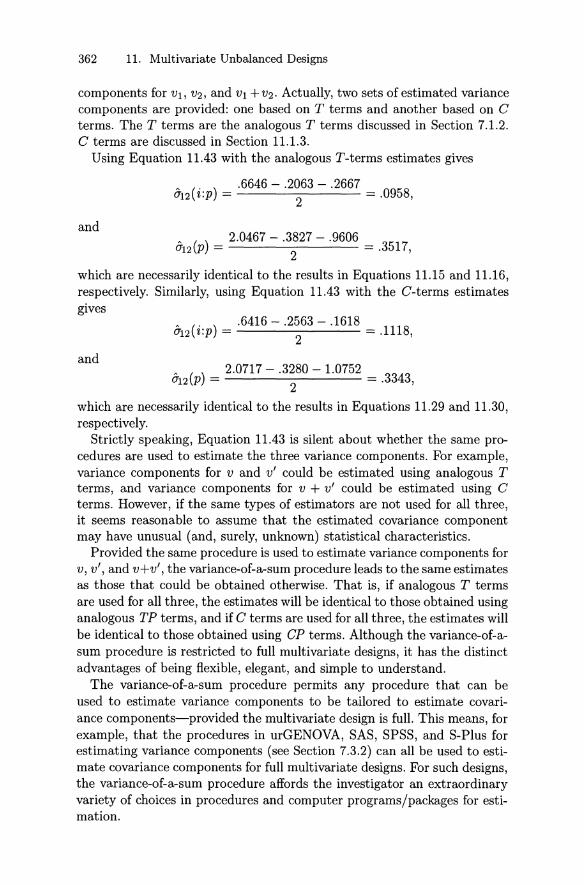
362 11. Multivariate Unbalanced Designs

components for VI, V2 , and VI +V2' Actually, two sets of estimated variancecomponents are provided : one based on T terms and another based on Cterms. The T terms are the analogous T terms discussed in Section 7.1.2.C terms are discussed in Section 11.1.3.

Using Equation 11.43 with the analogous T-terms estimates gives

~ ( ') .6646 - .2063 - .26670"12 up = 2 = .0958,

and~ () 2.0467 - .3827 - .9606 3 7

0"12 P = 2 = . 51 ,

which are necessarily identical to the results in Equations 11.15 and 11.16,respectively. Similarly, using Equation 11.43 with the C-terms estimatesgives

~ (" ) _ .6416 - .2563 - .1618 _ 11180"12 z.p - 2 - . ,

andaI2(p) = 2.0717 - . 3~80 - 1.0752 = .3343,

which are necessarily identical to the results in Equations 11.29 and 11.30,respectively.

Strictly speaking, Equation 11.43 is silent about whether the same pro­cedures are used to estimate the three variance components. For example,variance components for V and v' could be estimated using analogous Tterms, and variance components for v + v' could be estimated using Cterms. However, if the same types of estimators are not used for all three,it seems reasonable to assurne that the estimated covariance componentmay have unusual (and, surely, unknown) statistical characteristics.

Provided the same procedure is used to estimate variance components forv, v' , and v+v', the variance-of-a-sum procedure leads to the same estimatesas those that could be obtained otherwise. That is, if analogous T termsare used for all three, the estimates will be identical to those obtained usinganalogous TP terms, and if C terms are used for all three, the estimates willbe identical to those obtained using CP terms. Although the variance-of-a­sum procedure is restricted to full multivariate designs, it has the distinctadvantages of being flexible, elegant , and simple to understand.

The variance-of-a-sum procedure permits any procedure that can beused to estimate variance components to be tailored to estimate covari­ance components-provided the multivariate design is full. This means , forexample, that the procedures in urGENOVA, SAS, SPSS, and S-Plus forestimating variance components (see Section 7.3.2) can all be used to esti­mate covariance components for full multivariate designs. For such designs,the variance-of-a-sum procedure affords the investigator an extraordinaryvariety of choices in procedures and computer programsjpackages for esti­mation.

11.1 Estimating G Study Covariance Components 363

11.1.6 Missing Data

To this point, the discussion of estimating covariance components for un­balanced designs has given explicit consideration to designs that are un­balanced with respect to nesting only. Actually, however, the proceduresthat have been discussed can be used to obtain unbiased estimates of co­variance components when covariance components designs are crossed butunbalanced with respect to missing data, provided both v and v' have thesame pattern of missing data. Rarely, however, does the same pattern ofmissing data occur by chance. Usually, some data must be eliminated.

Consider, for example , the synthetic data for the p. x i· design in Ta­ble 11.7. This design is unbalanced in the sense that observations are miss­ing for pz and i4 on VI, for P3 and i s on VI, and for P7 and i4 on Vz. That is,there are two missing observations for VI, one missing observation for vz,and neither of the missing observations for VI corresponds to the missingobservation for Vz. Clearly, the patterns of missing data are different forVI and Vz . To make the missing data patterns the same, we can eliminatethe observations that correspond to the missing data. These are indicatedby an asterisk in Table 11.7. The reduced data set has 57 observations forboth VI and Vz .

One way to estimate the covariance components is to use the variance­of-a-sum procedure in Section 11.1.5. That is,

• use the analogous T terms procedure in Section 7.1.4 to estimate thevariance components for the unbalanced P x i design for VI , Vz, andVI + Vz, and

• use Equation 11.43 to estimate the covariance components.

Table 11.7 provides the analogous T terms and estimates of the variancecomponents. Using the latter in Equation 11.43 gives

1.6053 - .3977 - .4204 _ 39362 - .

.6713 - . 3~25 - .2675 = .0407

3.9982 - 1.2244 - 1.4906 = .6416.2

(11.44)

Alternatively, the covariance components can be estimated using anal­ogous TP terms (see Section 11.1.2), which are provided at the bottomof Table 11.7. The estimators of the covariance components are obtainedby replacing analogous T terms in Equation Set 7.17 with analogous TPterms. The resulting estimated covariance components are identical to thosecomputed above (see Exercise 11.8).

Eliminating data to obtain the same pattern of missing data for V and v'is potentially problematic. For example, doing so could result in a reduced

364 11. Multivariate Unbalanced Designs

TABLE 11.7. Synthetic Data Example for Unbalanced p. x i· Design

VI V2 VI + V2

P i l i2 i3 i4 is i6 il i2 i3 i4 is i6 il i2 i3 i4 is 26 np

1 6 4 3 5 4 4 6 4 5 6 4 5 12 8 8 11 8 9 62 3 2 2 5 5 6 4 5 * 2 5 9 6 7 7 10 53 6 5 7 5 3 6 5 8 4 * 3 12 10 15 9 6 54 4 2 2 3 3 5 5 4 2 4 3 5 9 6 4 7 6 10 65 4 4 3 5 4 6 4 5 5 3 3 7 8 9 8 8 7 13 66 8 5 4 7 5 4 9 6 6 5 7 7 17 11 10 12 12 11 67 5 4 5 * 4 4 4 5 6 4 5 9 911 8 9 58 4 5 3 4 5 6 6 7 6 6 5 6 10 12 9 10 10 12 69 7 5 4 6 6 5 6 7 3 5 5 6 13 12 7 11 11 11 6

10 5 3 3 7 4 5 6 5 4 6 2 6 11 8 7 13 6 11 6

ni 10 10 10 8 9 10 10 10 10 8 9 10 10 10 10 8 9 10Sum 52 39 36 42 40 47 58 52 50 39 35 55 110 91 86 81 75 102

VI V2 VI + V2

X 4.4912 5.0702 9.5614

T(p) 1181.3000 1500.3667 5329.5333T( i) 1171.2778 1485.5361 5263.2250T(pi) 1254.0000 1583.0000 5549.0000T(J.L) 1149.7544 1465.2807 5210.9649

0-2(p) .3977 .4204 1.60530-2(i) .3225 .2675 .67130-2(pi) 1.2244 1.4906 3.9982

Tp 9.5614 TH2(p) 1323.9333np 10

TH2(i)6 Ti = 5.7368 1303.2056nin+ 57 Ap 1.0093 TH2(pi) 1356.0000

Ai 1.0052 TH2(J.L) = 1279.9649

Not e. In the top part of the table, a blank ent ry indicates missing data , and an asteriskindicates data that are disregarded .

11.1 Estimating G Study Covariance Components 365

TABLE 11.8. Coefficients of JivJiv ' and Covariance Components in Expected Val-ues of CP Terms for p. x i · Design with Missing Data

Coefficients

E CP te rm J-lvJ-lv' <7vv' (p) <7vv' (i) <7vv' (pi)

E CPvv' (J-l ) 1 L npmp L nimi ---!I±....-p n+m+ i n+m+ n+m+

E CPvv' (p) n p n p L -q~ L - q~p npmp p npmp

E CPvv,(i ) L qi L qini niTi 'rnn ·m ·

. " i t. t,E CPvv,(pi ) q+ q+ q+ q+

Note. q+ is the total number of products of Xpiv and X piv ' such t hat neit her obse rvationis missing; qp is the number of items for person p such that neit her the resp onse for vnor the resp onse for v' is missing; and qi is the number of persons for item i such thatneither th e response for v nor the resp onse for v' is missing .

data set that is considerably smaller than the original one. Also, for theestimators to be unbiased, the missing data must be missing at random;that is, the pattern of missing data must be uncorrelated with the modeleffects. T his statement applies both to data that are truly missing (e.g.,t he t hree observations not present in Table 11.7) and to any data t hat areeliminated (e.g., t he t hree observations with an asterisk in Table 11.7). Thisassumption may be st rained in many real dat a contexts.

It is possible to der ive the expected values of CP terms without as­suming that missing data patterns are the same. For the pOx iO design ,the expecte d values are provided in Tab le 11.8. Although they are quitecomplex, they have t he advantage of using more of the data to est imatecovariance components than is used when data are eliminate d to create thesame pattern of missing dat a.

There are missing data situations that cannot be hand led easily by ap­plication of t he procedures discussed here. Consider, for example, the syn­thet ic data example of the p. x W:hO) design in Tab le 11.4, and supposet he response for PI , h1, and VI was missing, as well as t he response forP2 , h3 , and V 2 . The compound-means procedure could st ill be used in themanner indicat ed in Section 11.1.4 to est imate the covariance components.However , for the CP-terms procedure, the coefficients in Table 11.3 nolonger appl y, and th e expected values of the CP terms would have to bederived . Note also that in est imat ing the variance components, the analo­gous T terms would change, which means t hat the coefficients in Table 7.4and the est imators in Equation Set 7.14 no longer app ly. Of course, the ex­pected values of the analogous T terms can be derived and used to est imatethe variance components , but doing so is tedious.

366 11. Multivariate Unbalanced Designs

11.1. 7 Choosing a Procedure

For multivariate designs with a single linked facet, the covariances of ob­served mean scores are unbiased estimates of the covariance components.If the design is unbalanced, the investigator must choose between simplemeans or compound means, but otherwise there are no particular estima­tion ambiguities. For multivariate unbalanced designs with more than onelinked facet , however, ambiguities abound in selecting an estimation pro­cedure.

There are several statements that can be made about the principal pro­cedures that have been discussed in this chapter: the MP, TP, CP, andcompound-means procedures. First, they all give the same estimates forbalanced designs. Second, they require no assumptions about distributionalform. Third, they all give unbiased estimates. Fourth, other statistical char­acteristics of the estimates for the various procedures are generally un­known.i' It follows that there is no obvious statistical basis for choosingamong the procedures, and only ad hoc suggestions can be offered.

For balanced multivariate designs, there is historical precedent favoringthe MP procedure. It is essentially the procedure proposed by Cronbachet al. (1972) over a quarter century ago, and it is closely related to theANOVA procedure discussed in Chapter 3 for estimating variance com­ponents for balanced designs. For unbalanced designs, the TP procedureis not always applicable, but if it does apply, this procedure has the ad­vantage of being closely related to the analogous ANOVA procedure forestimating variance components that was discussed in Chapter 7. The CPprocedure is somewhat more complicated than the TP procedure, but theCP procedure has the distinct advantage of being applicable to any unbal­anced multivariate design. The compound-means procedure is a MP-likeprocedure that can be viewed as a covariance-components version of anunweighted analysis-of-means.

Of course , other procedures might be considered as weIl. Indeed , there areprobablyan unlimited number of quadratic-forms procedures that might beemployed. In particular, the variance-of-a-sum procedure makes numerousprocedures applicable to estimating covariance components for full multi­variate designs, including maximum likelihood and MINQUE procedures. Itseems likely that most of the strengths and weaknesses of these proceduresfor estimating variance components extend to covariance components, asweIl.

There is no theoretical requirement that the procedure used to estimatecovariance components must parallel that used to estimate variance com­ponents. For example, the CP-terms procedure could be used to estimatecovariance components and the analogous T-terms procedure could be usedto estimate variance components.

3This is a slight exaggeration, but it is true enough for the discussion here .

11.2 Examples of G Study and D Study Issues 367

For unbalanced multivar iate designs, there is always the alte rnative ofrand omly discarding data to obtain a balanced design. Indeed, for designsthat are unbalanced with respect to missing data, eliminating data is oneapproach that was explicitly discussed in Section 11.1.6 for estimating co­variance components. It was noted there, however, that this app roach canbe problemati c if it results in eliminating large amounts of data. Further­more, Chapter 8 illustrated t hat randomly discarding data to achieve abalanced design for esti mating variance components can be a questionablepractice. Since a multivariate design is a kind of conjunct ion of univariaterand om designs th at are linked through covariance components , t he st rat­egy of randomly eliminat ing data seems likely to be even more problemat icwhen applied to multivariate designs. Still , undoubtedly there are timeswhen this ad hoc approach is sensible, at least relative to other availablealternatives.

11.2 Examples of G Study and D Study Issues

The procedures for est imating covariance components discussed in Sec­tion 11.1 are illust rated here using real-dat a examples of several unbalancedmultivariate designs. This sect ion also illustrates numerous D st udy issues,including the est imation of D st udy covariance components . Two of theexamples discussed here involve two-facet table of specifications models.T hese examples employ the G st udy p. x W: hO) and p. x W: h· ) designsand the corresponding D study p. x (J0:HO) and p. x (1°: H· ) designs.T he third example uses the G st udy p" :(d· x 0·) design and the D st udyP" :(d· x 0· ) design to examine measurement characteristics of reading­minus-math difference scores for school districts.

11.2.1 ITBS Maps and Diagrams Test

In describing the p. x W: hO) design, Section 9.2.3 introduced the MD ex­ample, the Map s and Diagrams test ofthe Iowa Tests of Ba sic Skills (ITBS)(Hoover et al., 1993). For this test, there are two distinct typ es of stimulusmaterials, maps and diagrams, that are fixed condit ions of measur ementin the sense that every form of the Maps and Diagrams test contains bothtypes of st imulus mat erial. Specifically, for Forms K and L, Level 10, th ereare two maps and two diagrams. For each of the two maps there are sixand seven items, respectively; similarly, t here are six and seven items, re­spectively, for each of the two diagrams. The covariance components designis unbalanced because bot h of the variance components designs are unbal­anced; t hat is, there are different numbers of items nested within each ofthe two maps and different numbers of items nested within each of the twodiagrams.

368 11. Multivariate Unbalanced Designs

TABLE 11.9. G Study for Maps and Diagrams

Variance and Covariance Components

Mean Squares Estimates Standard Errors"

M p = [ .7299 .0354b ] ~p= [ .0404 .0354 ] [ .0030 .0028 ].0354b .6727 .0354 .0319 .0028 .0027

M = [ 161.6959 ] ~h = [ .0062.0001 ] [ .0060

.0018]h 68.4253

Mi :h =[ 43.9569 ] ~i:h = [ .0148

.0226] [ .0036.0047 ]66.8994

Mph= [ .2041.2578 ] ~ph = [.0032

.0116 ] [ .0001.0001 ]

Mpi:h = [.1832 ] ~ [ .1832 ] [ .0062 ]

.1831 ~pi:h = .1831 .0093

Note . Sampie sizes are: np = 2951 students, nh = 2 maps with 6 and 7 items in VI , andnh = 2 diagrams with 6 and 7 items in V2.

a Based on two replications.bObserved covariance.

For this test, Table 11.9 provides mean-square and mean-product ma­trices (M), as well as estimated variance-covariance matrices (~) , basedon the responses of 2951 students who took Form K in a standardizationstudy. In each matrix, the first row/ column is for maps and the second isfor diagrams.

Since the only linked "facet" is for the objects ofmeasurement (students),all entries in the M matrices are mean squares except for the off-diagonalelements of M p , which contain the observed covariance for students' mapsand diagrams scores based on simple means (see Equation 11.1). This ob­served covariance is an unbiased estimate of the covariance component formaps and diagrams. Since the two variance component designs are unbal­anced p x (i: h) designs, the mean squares are actually "analogous" meansquares, and formulas for estimating the variance components are given inSection 7.1.3.

When the standardization was conducted, both Forms K and L wereadministered to randomly equivalent groups of students, which permits usto obtain two estimates for each variance and covariance component. This,in turn, enables us to estimate standard errors for each of the components,as reported in the last column of Table 11.9. The standard error for a single

11.2 Examples of G Study and D Study Issues 369

estimat e is simply the standard deviation of the est imates, and when thereare only two replicates (say Xl and X 2 ) , the standard error (SE) formulais especially simple:

(11.45)

Consider , for example, the covariance component for persons . The FormsK and L estimates are o-vv,(p) = .0354 and o-vv,(p) = .0315, respectively.Therefore, the est imated standard error for any single est imate is:

A[A ( )] 1·0354 - .031510" O"vv' p = .j2 = .0028,

which is reported in Table 11.9. This estimate does not make any normalityassumptions. It can be compared to th e norrnality-based estimate for FormK that is obtained using Equation 9.55:

(.0561)( .0517) + (.0354)22952 = .0012,

whieh is almost 60% smaller than the est imate of the standard error thatdoes not make normality assumptions. For this dichotomous-data example,the empirieally based estimate of .0028 seems much more credible.

Table 11.10 provides results for a D study th at uses the same sam plesizes as the G study, and that assumes th at the w weights are proportionalto the sample sizes. The only complexity caused by the unbalanced nature~ this p. x ([0 :HO) des~gn invol;::,es the divisors of the elements of ~h and~ph required to obt ain ~H and ~pH , respectively. Because these matricesare diagonal, the elements under consideration are variance components,and the divisors are those discussed in Section 7.2.2 for the unbalancedunivariate p x (I :H ) design:

(11.46)

where h = 1, . . . ,n~ and n~+ = I:hn~:h' If all of the n~:h are the sameconstant for a given level of v, t hen n~ = n~ for th at level of v. Equa­tion 11.46 is the same as Equation 7.28, except for th e use of D studysample sizes. With n~:h sampie sizes of six and seven for both VI (maps)and V2 (diagrams), n~ = 1.988 for both levels of the fixed facet.

Once the D st udy est imated variance-covariance matrices are obtained,almost all of the D st udy methodology discussed in Chapter 10 can be ap­plied directly, whieh leads to the results at th e bottom of Table 11.10 . Two­replicat e est imated standard errors for the composite result s are providedin parentheses. These provide direct est imates of the st ability of quantitiessuch as E p2 .

370 11. Multivariate Unbalanced Designs

TABLE 11.10. D Study for Maps and Diagrams

D Study

G Study Components Divisors" Components

~ = [.0404 .0354]p .0354 .0319

~ = [ .0062 ]h .0001

~ [ .0143 ]:Ei:h = .0226

~ [ .0032 ]:Eph = .0116

~ [ .1832 ]:Epi:h = .1831

1.9881.988

13.00013.000

1.9881.988

13.00013.000

~ = [ .0404p .0354

~H = [ .0031

~I:H = [ .0011

~ _ [ .0016LJpH -

~ [ .0141LJpI:H =

.0354 ]

.0319

.0000 ]

.0017 ]

.0058 ]

.0141 ]

Composite Using Wl = W2 = .5

ab(r)

ab(8)

ab(ß)E p2

~

.0358 ( .0028b)

= .0089 (.0004b)

.0104 (.0006 b)

.801 (.020 b)

.775 (.003b)

~ = [ .0404 .9855C]

T .0354 .0319

~ = [ .0157 ]8 .0199

~ = [ .0200 ]A .0217

a D study sampie sizes are : nh= 2 maps with 6 and 7 items in VI , and nh= 2 diagramswith 6 and 7 items in V2 .

bEst imate d standard errors based on two forms .CDisat tenuated correlation.

Since the disattenuated correlation between the universe scores for mapsand diagrams is quite high (.986) , it is natural to consider what mighthappen to measurement precision for composite scores if a form of the testcontained only maps or only diagrams, even though the universe of gen­eralization remained unchanged with an equal weighting of maps and dia­grams. In principle, we could answer this question using either MSEc(ß)or MSEc(8) in Section 10.1.5. Here we use MSEc(8) , given by Equa­tions 10.37, because the various forms of MD are carefully equated, whichshould diminish , if not eliminate, the contribution of the variance compo­nents in the ~H and ~I:H matrices.

With Wl = W 2 = .5, MSEc(8) based on using two diagrams with sixitems and two diagrams with seven items is

MSEc(8) = ar(p) + a~(p) - 2 a12(p) [a~(Ph) a~(Pi :h)]4

+ - v-/-+ /nh n i +

11.2 Examples of G Study and D Study Issues 371

.0403 + .0319 - 2(.0354) ( .0116 .1831)4 + 3.9765 + 26

.0103,

which is about 15% larger t han ab(o) = .0089, although the absolute mag­nitude of t he difference is quite small. The corresponding result based onusing four maps is virtually indistin guishable from ab(o) = .0089.4

It certainly appea rs that there would not be much change in overallmeasurement precision if a form of the Maps and Diagrams t est had un­equal numbers of maps and diagrams , provided the total numb er of st imuliwas four and the tot al numb er of items was about 26. Of course , thereare ot her reasons for using equal numb ers of maps and diagrams, not theleast of which is that doing so faithfully reflects the intended universe ofgeneralizat ion.

Another matter that might be considered is the measurement precisionof a half-length form of t he Maps and Diagrams t est . This is not as simplean issue as it may appea r, however , because there are a number of possibleinterpret ations of "half-lengt h'' for t his test , such as

1. half of the passages, in t he sense of one map with six items and onediagram with seven items; and

2. half of the items per passage, in the sense of two maps with threeitems each, and two diagrams with three and four items.

Th ese would be half-Iength forms in t hat they both involve half (13) of t henumber of items in a full-length form (26).

Results for t hese two possibilities are provided in t he l~ft and right sides,respectively, of Table 11.11. T he divisors that give the ~H and ~pH ma­t rices are the n;' given by Equation 11.46, but ot herwise t he computationsare straight forward. It is evident that using all four passages with half ofthe items per passage leads to somewhat great er measurement precisionthan using half of t he passages. Roughly, error variances are 10 to 12%lower , coefficients are 3 to 4% higher, and signal-noise ratios are 13 to 14%higher using all of the passages with half of the items per passage. Thecrux of the explanat ion for thi s difference is that using all of the passagesleads to lower values for t he est imated variance components in t he IjH andIj pH matrices. The differences associated with these two!erspec~ves on"ha lf-length" are not very large because the elements of ~h and ~ph arerelatively small.

There are ot her inte rpretations of "half-lengt h" that might be consid­ered. In par ticular, length might be viewed with respect to t he amount oft ime needed to complete the test. From this perspective, using half of the

4Computations using Form L give similar res ults.

372 11. Multivariate Unbalanced Designs

TABLE 11.11. Half-Length D Studies for Maps and Diagmms

Half of the Passages" Half of the Items per Passage"

Divisors Components Divisors Components

~ = [ .0404 .0354 ] ~ = [ .0404 .0354 ]p .0354 .0319 p .0354 .0319

1.000 ~H = [ .0062.0001 ]

2.000 ~H = [ .0031.0000 ]1.000 1.960

6.000 ~ _ [ .0025.0032 ]

6.000 ~I:H = [ .0025.0032 ]7.000 I :H - 7.000

1.000 ~ _ [ .0032.0116 ]

2.000 ~ _ [ .0016.0059 ]1.000 pH - 1.960 pH -

6.000 ~ _ [ .0305.0262 ]

6.000 ~pI:H = [ .0305.0262 ]7.000 pI:H - 7.000

~ = [ .0404 .9S55 C] ~ = [ .0404 .9S55 C]

T .0354 .0319 T .0354 .0319

~o = [ .0338.0377 ]

~o = [ .0322.0321 ]

~L'. = [ .0424.0410 ]

~L'. = [ .0377.0353 ]

Composite Defined Using Weights of Wl = W2 = .50

a-b(T) = 0.0358 a-b(T) = 0.0358a-b(8) = 0.0179 a-b(8) = 0.0161

a-b(ß) = 0.0209 a-b(ß) = 0.0183

Eß2 = 0.667 Eß2 = 0.690

<I> = 0.632 <I> = 0.662

§i!l(8) = 2.001 §i!l(8) = 2.228

8jN(ß) = 1.714 8jN(ß) = 1.958

aD study sampie sizes are : n~ = 1 map with six items in VI , and n~ = 1 diagramwith seven items in V2.

bD study sampie sizes are : nh = 2 maps with three and three items in VI , and nh = 2diagrams with three and four items in V2 .

CDisat tenuated correlations.

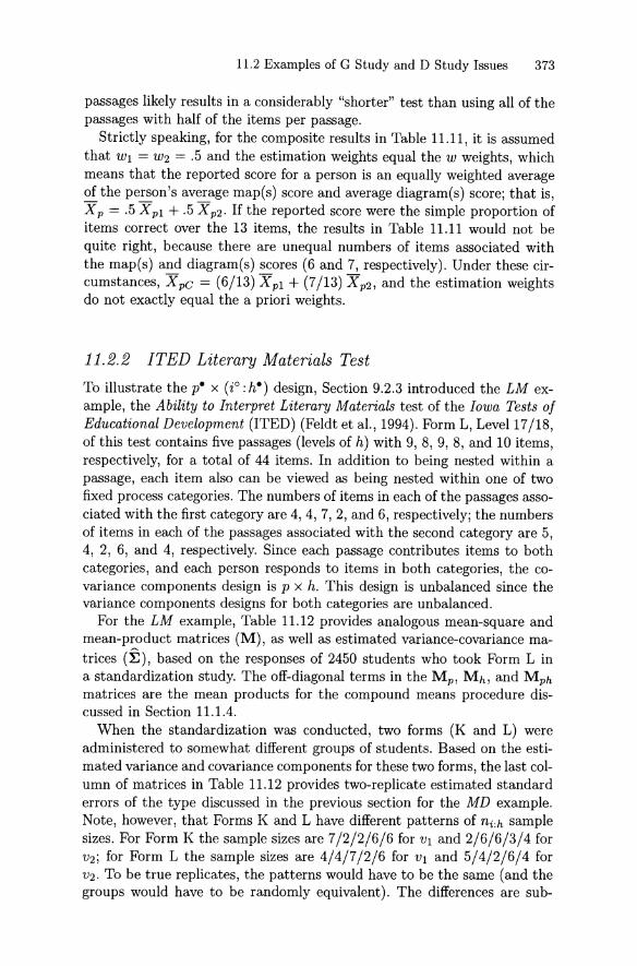
11.2 Examples of G Study and D Study Issues 373

passages likely results in a considerably "shorte r" test than using all of thepassages with half of t he items per passage.

Strictly speaking, for the composite results in Table 11.11, it is assumedthat Wl = Wz = .5 and t he est imation weights equal the W weight s, whichmeans that the reported score for a person is an equally weighted averageof t he person 's average map(s) score and average diagram (s) score; t hat is,X p = .5 X p 1 + .5 X pz. If t he report ed score were t he simple proportion ofitems correct over t he 13 items, the results in Table 11.11 would not bequite right , because there are unequal numbers of items associa ted withthe map (s) and diagram (s) scores (6 and 7, respectively). Under these cir­cumstances, X pc = (6/13) X p l + (7/ 13) X pz, and the est imation weightsdo not exactly equa l the a priori weights.

11.2.2 ITED Literary Materials Test

To illustrat e the p. x W:h· ) design, Section 9.2.3 introdu ced the LM ex­ample, the Ability to Int erpret Literary Mat erials test of the Iowa Tests 01Edu cational Developm ent (IT ED) (Feldt et al. , 1994). Form L, Level 17/18 ,of this test contains five passages (levels of h) with 9, 8, 9, 8, and 10 it ems ,respect ively, for a total of 44 items. In addit ion to being nested within apassage, each item also can be viewed as being nested within one of twofixed process catego ries. T he numbers of items in each of the passages asso­ciate d with the first category are 4,4, 7, 2, and 6, respectively; t he numb ersof items in each of the passages associated with t he second category are 5,4, 2, 6, and 4, respectively. Since each passage cont ributes items to bothcategories, and each person responds to items in both categories, the co­variance components design is p x h. This design is unbalanced since thevariance components designs for both categories are unbalanced.

For t he LM example, Table 11.12 provides analogous mean-square andmean-product matri ces (M), as well as estimat ed variance-covariance ma­trices (f:) , based on the responses of 2450 st udents who took Form L ina standardizat ion study. The off-diagonal terms in the M p , Mh , and Mphmatrices are the mean products for the compound means procedure dis­cussed in Section 11.1.4.

When the standardization was conducted, two forms (K and L) wereadministe red to somewhat different groups of students. Based on the esti­mat ed vari ance and covariance components for these two forms, the last col­umn of matrices in Table 11.12 provides two-replicat e est imated st andarderro rs of the type discussed in the previous section for the MD example.Note, however , that Forms K and L have different pat terns of ni:h samplesizes. For Form K t he sample sizes are 7/2/2/6/6 for VI and 2/6/6/3/4 forVz ; for Form L the sam ple sizes are 4/4/7/ 2/ 6 for VI and 5/4/ 2/6/ 4 forVz . To be t rue replicates, t he pat terns would have to be t he same (and thegroups would have to be randomly equivalent). The differences are sub-

374 11. Multivariate Unbalanced Designs

TABLE 11.12. G Study for Literary Materials Based on Mean Squares and MeanProducts

Analogous Mean Squares

and Mean Products"

Variance and Covariance Components

Estimat es Stand ard Errors''

M = [105.4833 2.1558 ]h 2.1558 43.7483

.1798] !:Pi :h = [ .1531 .1798]

.0018 .0009]

.0009 .0011

.0059 ].0057

.0047 .0010 ]

.0010 .0020

.0009 ].0013

[.0010 .0028 ].0028 .0030

[

[

[

[

.0087 .0009]

.0009 .0000

.0143 .0083]

.0083 .0089

.0046 ].0180

[.0443 .0405 ].0405 .0401

[

[

[

:Ep =

.0083 ]

.2163

.2109 ]1.0630

.2167

.0083

.1531

[11.3881 ]

44.2438

[

[1.2473

M , = .2109

M pi :h = [

Note. SampIe sizes for Form L are: n p = 2450 st udents and n h = 5 passages wit h 4, 4,7, 2, an d 6 it ems in VI, and 5, 4, 2, 6, an d 4 ite ms in V2.

aO ff-diagonal elements are mean produc ts for compound means pro cedu re.bBased on two repli cat ions.

stant ial enough to cast some doubt on the estimat ed standard errors. Still ,they are the only readily available est imates."

In Table 11.12, analogous mean squares are used to est imate variancecomponents (see Equ ation Set 7.14), and the compound means procedureis employed to estimat e covariance components. By cont rast, in Table 11.13C t erms are used to est imate variance components, and th e CP-terms pro­cedure is employed to estimate covariance components (see Section 11.1.3) .The est imated standard errors in Table 11.13 are analogous to those inTable 11.12.

Using the estimated standard errors as benchmarks , we observe thatalmost all of the Form L est imates in !:h , !:i :h' and !:ph based on C andCP t erms are substantially different from those based on analogous MBand MP t erms. Also, it is evident that the estim at ed standard errors of theelements of ~h , ~i :h , and ~ph based on C and CP te rms are noticeably

5T he previously discussed normality-based procedures for estimating standard errorsof estimated variance components (see Section 6.1.1) and est imated covar iance compo­nents (see Section 9.4.3) do not app ly to unbalanced designs.

11.2 Examples of G Study and D Study Issues 375

TABLE 11.13. G Study for Literary Ma teria ls Based on C Terms and CP Terms

C Terms Variance and Covariance Components

and CP Terms Estimat es Standard Errors"

Cp = [ 1216.10 1027.41 ]~p = [ .0452 .0430 ] [ .0003 .0018 ]

1027.41 904.70 .0430 .0409 .0018 .0035

C h = [ 2.27693 1.84766 ] ~h = [ .0180 - .007] [ .0132 .0111 ]1.84766 1.53788 - .007 - .026 .0111 .0333

C i :h = [ 10.42567.0525 ] ~i :h = [ .0029

.0388 ] [ .0035.0301 ]

C ph = [ 6753.88 5124.37 ]~ph = [ .0097 .0059 ] [ .0042 .0016 ]

5124.37 4937.70 .0059 .0045 .0016 .0028

C pi :h = [37470 ] ~ [ .1568

.1834 ] [ .0023.0089 ]29044 ~pi : h =

Note. Sampie sizes for Form L are: n p = 2450 students and nh = 5 passages with 4, 4,7, 2, and 6 items in VI, and 5, 4, 2, 6, and 4 items in V2 .

a Based on two replications.

larger those based on analogous MB and MP t erms . It seems plausiblethat t hese differences in est imate d standard errors are at t ributable, at leastpartly, to the rather severely unbalanced nature of the design, coupled witht he fact that the sampie size patterns for Forms K and L are quite different.There is at least t he hint of a suggest ion that est imates based on C andCP terms te nd to be more variable t han t hose based on analogous MB andMP te rms.

These observations do not provide unequivocal guidance for a choice ofestimat es, but t here are pragmatic reasons for choosing t he est imate s basedon t he analogous MB te rms and MP terms :

• t he variance-component est imates based on analogous MB terms havemore precedent than those based on C terms; and

• t he covariance-component est imates based on the compound-meanspro cedure are simpler to concept ualize and compute.

Note also that t he compound-means procedure does not explicit ly incor­porate t he n~:h sampie sizes. This may be somewhat defensible for thisexa mple in that Forms K and L of Literary Materials have subst antiallydifferent sampie size pat t erns, even t hough t he two forms are used inter­changea bly (after equat ing).

376 11. Mult ivariate Unbalanced Designs

TABLE 11.14. D Study for Literary Materials Using G Study Estimates fromTable 11.12

D Study"

G Study Components Divisors" Components

~ = [ .0443 .0405 ]~p = [ .0443 .0405 ]

p .0405 .0401 .0405 .0401

~h = [ .0087 .0009 ] 4.372~H = [ .0020 .0002 ]

.0009 .0000 4.546 .0002 .0000

~i : h = [ .0046.0180 ]

23.000~I :H = [ .0002

.0009 ]21.000

~ [ .0143 .0083 ] 4.372 ~ [ .0033 .0015 ]~ph = .0083 .0089 4.546

~pH =.0015 .0020

~ . _ [ .1531.1798 ]

23.000~pI :H =

[ .0067.0086 ]pt:h - 21.000

Composite: Wl = .523; W2 = .477~T= [.0443

.96141

a-b(r) = .0415 (.0033C) .0405 .0401

a-b(o) .0059 (.0003C)

~6 = [ .0099.14441

a-b(ß) .0067 (.0007C) .0015 .0105

Eß2 .876 (.012 C)

~~ = [.0121 .1391J

cI> .861 (.021C) .0016 .0114

QD study sampIe sizes are: nh = 5 passages with 4, 4, 7, 2, and 6 items in VI, and 5,4, 2, 6, and 4 items in V2 .

bFor covariance components in EH and EpH, the divisor is 5.616.CEst imated standard errors based on two forms .dDisattenuated correlations.

The G study estimated variance and covariance components based onanalogous MB and MP terms in Table 11.12 are used in Table 11.14 toestimate results for a D study with the same sample sizes as the G st udy,with W weights proport ional to sample sizes, and with estimation weightsequal to w weights. To obtain the D study variance component estimates,the G st udy estimates are divided by nh given in Equation 11.46 . The D

study covariance component estimates in ~H and ~pH are obtained usingthe divisor:

(11.47)

11.2 Examples of G Study and D St udy Issues 377

where h = 1, . . . ,nh,n~:h are the D study sample sizes for v, m~:h are the Dstudy sample sizes for v', n~+ = L h n~:h ' and m~+ = Lh m~:h ' (Note thatnh

v v' would be nh if all of the n~:h and the m~:h were th e same constant .)

To prove that Equ ation 11.47 is the divisor of avv,(h) , recall th at theconvent ion adopted in thi s book is that u designates effects associated withlevel v, and ~ designates effects associated with level v' . Also, to simplifynot ation, suppose th e G and D study sample sizes are the same. Then

avv,(H) = E [(Lh::hVh ) (Lh;::h~h )]

n . ~ . E [2: ni :hmi:h( vh~h) + 2: 2: ni :hmi :h'(Vh~h')]t+ t+ h hf.h'

Since EVh~h' = 0 for h i= h' , it follows that

avv,(H )

An entirely analogous proof applies for avv,(pH), and similar proofs applywhen the G and D study sample sizes are different .

For the LM example, recall th at the ni:h were 4, 4, 7, 2, and 6 itemsfor VI , and the corresponding m i:h were 5,4, 2, 6, and 4 items for V2 . Thisgives

v I 23 x 21nh = = 5.616.

1 2 20 + 16 + 14 + 12 + 24

Once the D study est imated variance and covariance matrices are deter­mined, the remaining D study result s in Table 11.14 are easily obt ained inthe usual manner. Both relative and absolute errors for the two categoriesare slightly correlated (about .14), but universe scores are very highly cor­related (about .96). Such a high correlation indicates th at universe scoresfor the two categories are nearly linearly related, but this does not meanthat the categories should be ignored in test development. For example,if the universe of generalizat ion remained unchanged, but all items wereselected from the first category and the estim ation weights were set ata l = 1 and a2 = 0, then MSEc(8) = .0071, which is about 20% larger th ana-b (8) = .0059.

For the LM example, overall absolute error variance for the pe X (J0:He)design is a-b (6.) = .0067. Both conceptually and computationally, this isequal to the average of the condit ional absolute error variances for each ofthe 2450 persons in the sample. For any person , condit ional absolute errorvariance is the variance of the mean for the with in-person JO

: He design, in

378 11. Multivariate Unbalanced Designs

0.90.80.70.4 0.5 0.6MeanScore

0.30.20.1

CSEM

Lord's• CSEM

Fitted : :.. CSEM . . ::

0.20

0.18

0.16

:::E 0.14~

CI) 0 12«l'§ 0.10

.;::.a 0.08su 0.06

0.04

0.02

0.00 -+-r"""""'''T'""T'"T""T'"''''''''''r-T""'T"''T""'T'''''''''''''T'""T'"-r-r-....,-r-T""'T"''T""'T'''''''''''''T'""T'"T""T'"'''''-r-T""'T"''T""'T''''''''''"'T""T'""T""'l'''"'''''-''''

o

FIGURE 11.1. Conditional absolute standard errors of measurement for LiteraryMaterials for 494 examinees.

the sense discussed in Section 10.2.3 (see also Exercise 11.12). Figure 11.1provides a plot of conditional SEMs, ac(ßp ) , for nearly 500 examinees,along with a quadratic fit to the conditional SEMs for all 2450 examinees."Also plot ted are Lord 's conditional SEMs in which all 44 items in LiteraryMaterials are assumed to be sampled from an undifferentiated universe;that is,

It is evident from Figure 11.1 that this simplistic model substantially un­derstates the magnitude of the conditional SEMs.

Thus far in this section, results have been presented only for Form Lof Literary Materials. There are other forms, one of which is Form K.These forms are developed according to the same specifications, to theextent possible. However, Forms K and L have different patterns of numbersof items within passage for the first process category and for the secondpro cess category. Such dissimilar patterns are common-indeed, almostinevitable-in passage-based tests with process categories constituting partof a table of specifications for forms. Test developers may be able to achievesome degree of balance across categories, but seidom is the pool of availablepassages so rich that the same patterns of sample sizes can be used acrossforms .

6The quadratic fit to the error variances for all 2450 examinees is given by the poly­

nomial equation o-b(~p) = - .0038 + .0537 Xpc - .0529 X~c . The square roots of thesefitted values are given by the solid triangl es in Figure 11.1.

11.2 Examples of G Study and D Study Issues 379

Using n~ : h and m~:h to designate sampie sizes for Categories 1 and 2,respectively, sample-size stati stics for Forms K and L are given in the fol­lowing table.

Category 1 Category 2

Form n~ :h n~+v i

m~:h m~+v i V I

n h n h nh 12

K 72266 23 4.101 266 34 21 4.366 6.037L 44726 23 4.372 54264 21 4.546 5.616

Both forms have 23 items in Category 1 and 21 items in Category 2, whiehmeans that w weights will be th e same for the two forms when the weightsare prop ortional to the numbers of items within categories. However, thedissimilar sample-size patterns cause the two n~ and n~12 to be differentacross forms. For this reason, Forms K and L in th e LM example mighthave somewhat different psychometrie characterist ics even if, in all otherrespects , the forms were perfectly parallel.

Dissimilar sampie size patterns are perhaps inevitable, but they are stilla reflection of less than ideal experimental cont rol in test development.Furthermore, differences in sampie size patterns highlight an issue in con­ceptualizing replications of the measurement procedure. Strictly speaking,randomly parallel instances of the measurement procedure have the samesampie size patterns. That is, sampie sizes are not random effects . Rather ,both in est imat ion procedur es and in conceptualizing replications, sampiesizes are fixed effects.

Let us consider three possible sample-size patterns that might be usedfor the LM example:

1. sample-size patterns used in Form K;

2. sample-size patterns used in Form L; and

3. approximately constant sampie sizes (e.g., 4, 4, 5, 5, and 5 items forVI , and 4, 4, 4, 4, and 5 items for V2 ) '

Let us suppose, as weil, th at "ideal" forms would be built according to theth ird set of specifications.

For all three sample-size patterns, composite universe score variance isnecessarily the same, because universe scores are not affected by D studysampie sizes. Error variances, however, are different . The D study results inTable 11.14 assurne that th e universe of generalizat ion corresponds to thefirst set of sample-size patterns , although we are arguing hypothet ieallyth at "ideal" forms would be created according to the third set . Conse­quently, for some purposes, it might be sensible to consider the expectedcorrelat ion between a randomly selected form with Form K sample sizes(say X) and a randomly selected form with "approximately constant" sam-

380 11. Multivariate Unbalanced Designs

ple sizes (say X) :

where the first expected-observed-score-variance is for X and the second isfor X. The value of this correlation is necessarily somewhere between E p2

for the Form K sampIe sizes and E p2 for the "ideal" sampIe sizes.For the LM example, this theoretical argument is moot because there is

virtually no difference in composite relative error variances for the universes(assuming the G study est imate d variance and covariance components inTable 11.12 are the parameters). Still , in other contexts, consequential dif­ferences might be observed. In any case, it bears repeating that samplesizes are fixed conditions of measurement in generalizability theory.

11.2.3 Distriet Mean Difference Scores

Table 11.15 provides raw score summary statistics for Reading Comprehen­sion (R) and Math Total (M) grade equivalent scores on the lowa Tests0/ Basic Skills (ITBS) for fourth-grade students in a sampIe of 103 Iowaschool districts that tested in four consecutive years in the 1990s. For eachyear , the summary st atistics reported are for the distribution of unweighteddistrict mean scores. For exa mple, t he mean of 4.5961 for Reading Com­prehension in 1995 to 1996 was obt ained by comput ing the mean gradeequivalent score for st udents in each of t he 103 districts, and t hen comput­ing the mean (unweighted) of these means. The numb er of st udents in thedistricts ranges from 10 to over 600, with arithmet ic means for each of thefour years in the low 70s, and harmonie means in the 30s (see Table 11.15).

For any given year , the dat a provided in Table 11.15 do not provide abasis for generalization in that the data were collected on the same occa­sion using the same form of the ITBS.7 Across years , however , differentstudents were involved each year and two different forms were employed.So, variability in the Reading Comprehension and Math Tot al st atisticsover years reflects variability in both a person facet and an item facet.

G Study Design

One approach to examining t he issue of the generalizability of these district(d) mean scores over forms and years begins with an analysis employinga G st udy multivariat e p" :(d· x 0·) design, where p designat es students

7Dist ricts can choose when t hey ad minister the ITBS ; some test in the Fall and somein t he Spring. The data reported in Ta ble 11.15 are for districts t hat chose to test in t heFall .

11.2 Examples of G Study and D Study Issues 381

TABLE 11.15. Grade-Equivalent Scores for District Means Example

Year Form Test Mean S.D. T Sdiff HMan tot

1995-96 K R 4.5961 .5231 .7011 .3828 36.26 7656M 4.3823 .4528

1996-97 L R 4.5715 .5339 .7728 .3499 32.31 7252M 4.4039 .5000

1997-98 K R 4.4511 .5911 .8181 .3427 33.99 7397M 4.2758 .5272

1998-99 L R 4.4384 .5946 .8413 .3228 32.41 7386M 4.3324 .5303

Over Years R 4.5106 .4541 .8610 .2338 33.67b 29691M 4.3483 .4274

aHarmonic mean of number of students within each district.bHarmonic mean over districts of harmonie means over oceasions within distriet.

within districts (d), with each student tested in one of four years or occa­sions (0). Not e that t his representation ofthe design involves a complicate dconfounding of years and forms in what is being called t he "occasion" facet.

For this design , the levels of the fixed facet are Reading Comprehensionand Math Total grade-equivalent scores. This is an unb alanced multivari atedesign in that t here are different numbers of st udents wit hin districts, andthe design is full in the sense t hat t here are R and M scores for all district s,for all students within districts , and for all four years.

The seeond and third eolumns of Table 11.16 provide est imate d vari an cecomponents for R and M , respectively, using the analogous-ANOVA pro­cedure in Section 11.1.2 . Since this is a full multivari ate design , covariancecomponent s can be obtained using t he variance-of-a-sum pro cedure dis­cussed in Section 11.1.5. To obt ain them, the fourth column of Table 11.16provides est imat ed vari ance components for the sum of Rand M .8 Theest imated covariance components based on Equ ation 11.43 are in the fifthcolumn.

The patterns are very similar for the estimated variance components forR , the est imat ed var ian ce component s for M, and the est imate d covariancecomponents. Students account for most of the variance and covariance,occasion differences (i.e., year / forrn) are of little consequence, and there isevidence of variability and covariability in district mean scores.

At the bottom of Table 11.16, the est imated vari ance and covariance ma­trices are provided , with t he upper-diagonal elements being disattenu ated

8The estimated variance components for R, M , and R + M were obtained usingurGENOVA.

382 11. Multivariate Unbalanced Designs

TABLE 11.16. G Study for District Means Example of p" :(d· x 0·) Design forReading Comprehension and Math Total Grade-Equivalent Scores

Effect

dodop :do

.1668

.0038

.01783.3461

.1398

.0014

.01802.1765

.5791

.0097

.06019.0997

.1363

.0022

.01211.7886

.8925

.9529

.6772

.6628

.0340

.0008

.01161.9455

.1668

.1363

.0178

.0121

.8925 ].1398

.6772 ].0180

.0038

.0022

3.34611.7886

.9529 ].0014

.6628 ]2.1765

Note. It alicized values are disat tenuated corre lat ions.

correlat ions- all of which are quite large.9 Interpreting these correlat ionsrequires some thought. For example, consider PRM(d) = .89. This is theestim at ed correlation between Reading and Math Total grade-equivalentmean scores for districts, where each such mean is over students, forms,and years. Also, consider PRM(O) = .95. This is the est imated correlationbetween Reading and Math Total grade-equivalent mean scores for occa­sions, where each such mean is over st udents and districts. The fact thatPRM(d) is somewhat smaller th an PRM (O) suggests th at district mean scoresfor R and M are not as highly correlated as occasion (i.e., year / form) meanscores.

The st udent correlat ion PRM(p:da) = .66 is not a disattenuated corre­lat ion in the usual sense of that term. It is interpretable as an est imateof the correlat ion between Rand M for students in a randomly selecteddistrict for a randomly selected occasion. This correlat ion is essent ially anobserved score correlation, not an est imate of the correlat ion between Rand Muniverse scores for students. At the student level, there is only oneobservat ion for Rand one observation for M in these data, so there is nostat ist ical basis that permits generalizing student observed scores to uni­verse scores for R and M . Generalization is possible for district mean scoresbecause there are district scores for different forms and different years (and,therefore, different samples of st udents, too).

Note also th at PRM(do) and PRM(p:do) are almost identical (about .67).Apparently, the district-occasion interaction effects for R and Mare aboutas highly correlated as the observed student scores for R and M , but these

9The size of t hese corre lations is partly attribut ab le to scaling issues, but not entirely.

11.2 Examples of G Study and D St udy Issues 383

eorrelat ions are both eonsiderably smaller than the distriet means disat­tenuated eorre lat ion of .89.

D Study Design and Sampie Sizes

With dist riets as t he objeets of meas ure ment , t he D study mult ivari at edesign is P" :(d· x 0· ). Sinee t he design is full , for eaeh of the four matriees,t he D study sample-size divisor of t he G study varianee and eovarianeeeomponents is t he same. It is obvious t hat t he divisor is n~ for t he elementsof 1:0 and l:do' Less obviously, we use n~ii~ as t he divisor for the elements of

1:p:do , where ii~ is the harmonie mean (over distriets) of t he ii~:d (harmoniemean over oeeasions of t he n~:d within a distriet ) , as diseussed next.

Consider , for example, aRM(P:dO) , und er the simplifying assumpt ionthat G and D study sample sizes are the same. By definition ,

(~L _1_) aRM(p:do)n o 0 np:do

aRM( p:do)

noiip:d

where iip:d is the harmonie mea n of t he np:do wit hin a dist riet :

(11.48)

The result in Equation 11.48 is for a randomly seleeted distriet, and it iseondit ional on the harmonie mean iip:d . The average value over all distrietsis

~L aRM ~.p : do) = aRM(~:do ) ,n d d nonp:d n onp

where iip is t he harmonie mean (over districts) of the iip:d. Therefore, formany purposes we use

(11.49)

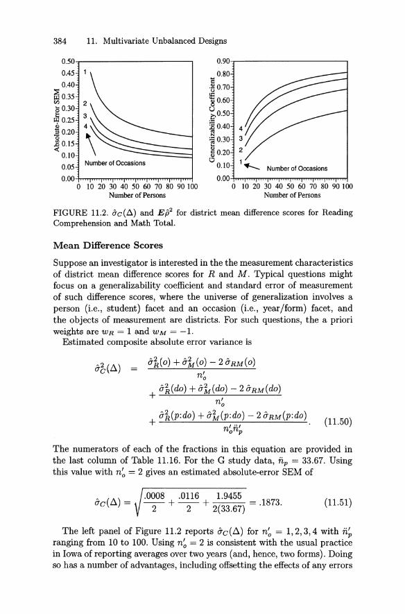
384 11. Multivariate Unbalanced Designs

0.50-r----------___,

0.45 1

0.40

~0.35CIl 28 0.30

~ 0.25 3B 4..3 0.20oE 0.15<

0.100.05 Number 01 Occasions

O.OO4,-,-..,..,..,.,..,..,.,..,.,.,.,.,..,.,.,.."..,.,..,.".,....,.,..'TTTTTTTT'I.........,,,...,...jo 10 20 30 40 50 60 70 80 90 100

Number of Persons

0.90~---------___,

0.80;::'Ö0.70...:'8 0.60u0 0.50

] 0.40 4s~ 0.30 3l:l 2~ 0.20

o 0.10 1.......... Number 01 Occasions

O.OO-lrn.,.,.,.,.,..,..,..,.,..,..,.,..,'T'l'T"""""""""""TTTT'I'TTTTTTTT'I""",",o 10 20 30 40 50 60 70 80 90 100

Number of Persons

FIGURE 11.2. ac(ß) and Er? for district mean difference scores for ReadingComprehension and Math Total.

Mean Difference Scores

Suppose an investigator is interested in the the measurement characteristicsof district mean difference scores for Rand M. Typical questions mightfocus on a generalizability coefficient and standard error of measurementof such difference scores, where the universe of generalization involves aperson (i.e., student) facet and an occasion (i.e., year/form) facet, andthe objects of measurement are districts. For such questions , the aprioriweights are WR = 1 and WM = -1.

Estimated composite absolute error variance is

The numerators of each of the fractions in this equation are provided inthe last column of Table 11.16. For the G study data, iip = 33.67. Usingthis value with n~ = 2 gives an estimated absolute-error SEM of

o-c(t::.) = .0008 + .0116 + 1.9455 = 18732 2 2(33.67) ' .

(11.51)

The left panel of Figure 11.2 reports o-c(t::.) for n~ = 1,2,3,4 with ii~

ranging from 10 to 100. Using n~ = 2 is consistent with the usual practicein Iowa of reporting averages over two years (and, hence, two forms) . Doingso has a number of advantages, including offsetting the effects of any errors

11.2 Exa mples of G Study and D Study Issues 385

that may be present in the equating of Forms K and L, and par t iallyoffsetting unusua l resul ts for districts with small num bers of st udents . Itis clear from Figure 11.2 that using two years' worth of data substantiallyreduces the absolute-error SEM for the difference in mean scores over whatit would be if only one year's data were used.

Estimated com posite universe score variance for districts is

o-b(d) = o-h(d) + o-1r(d) - 2 o-RM(d) = .0340,

where it is to be emp hasized that d stands for "dist rict" not "difference."Esti mated relat ive error variance is

o-h(do) + o-1r(do) - 2 o-RM(do)

n~

o-h(p:do) + o-1r(p:do) - 2 o-RM (P:do)+ '''' .non p

(11.52)

For n~ = 2 and ii~ = 33.67 (t he value in t he G st udy dat a) , o-b(J) = .0347and

E ·2 = .0340 = .495.p .0340 + .0347

(11.53)

T he right panel of F igure 11.2 reports E ß2 for n~ = 1, 2, 3, 4 and ii~ rangingfrom 10 to 100.

At least some approaches to est imat ing t he reliability of district meandifference scores would assurne uncorrelated erro rs. For t his example, giventhe magnitude of the covariances between the effects for R and M (seeTable 11.16), such an assumption would lead to seriously underestimatingreliability. Für example, assuming aRM(do) = aRM(p:do) = 0, n~ = 2, andii~ = 33.67, it is easi ly ver ified t hat E ß2 = .254, which is about half aslarge as t he value t hat incorporates correlated effects (.495) .

As another perspective on this example, note t hat the observed-sco revariances for each of t he four occasions (t he square of t he Sdiff values inTable 11.15) are .1466, .1224, .1175, and .1042. The average of these ob­served vari ances, .1227, is c1early an est imate of expected observed scorevariance for a single occasion. It follows that one est imate of a generaliz­ab ility coefficient for n~ = 1 and t he n p:do sample sizes in t he G st udy datais

E ·2 = .0340 = .2771p .1227 '

(11.54)

which is an estimated generalizab ility coefficient for a single occasion. Fort his example, t he Spearrnan-Brown formula applies (see Exercise 11.13)and can be used wit h Eq uation 11.54 to obtain an estimated generalizabilitycoefficient for mean scores over two occasio ns:

E•2 2( .2771)P = = .434

1.2771 '(11.55)

386 11. Multivariate Unbalanced Designs

. . . ..... : .. ~.. :. -... ""',.,. .,.. '..-:... ~)\-. ~• c·· ....-,- , .. . .

~ ~ ~ ~ 0 N V ~ 00 0 ~

9 9 9 9 0 0 0 0 0 ~

Mean Differences (1995--97)

1.2-.------------,

~ 1.0

'"q- 0.8~g; 0.6

S' 0.4..s 0.2e~ 0.0....s -0.2

~ -0.4

~ -0.6

-0.8 +n-......,..,.......,..,.................TTT"'TTT"'TTT"'"TTT""TTT"....-l

1995--991997--991995--97

0.7-r-------------,

0.6

~ 0.5

~ 0.4

~ 0.3g~ 0.2~6 0.1

~ O.O-r--......_r-,---..,..~ -0.1

-0.2

_0.3..1-------------1

FIGURE 11.3. Box plots and scatterplot for district mean difference scores.

which is associated with ab(o) = .0443. The discrepancy between the es­timated generalizability coefficients in Equations 11.53 and 11.55 is at­tributable primarily to the fact that the error variance in Equ at ion 11.53 isbased directly on analogous-ANOVA estimates of variance and covariancecomponents , whereas the error variance in Equ ation 11.55 is not .

As an additional perspective, note that the correlat ion (over district s)between the average of the difference scores for the first two years (1995- 96and 1996-97) and the average of the difference scores for t he last two years(1997-98 and 1998-99) is

r (1995-97, 1997-99) = .434. (11.56)

Figure 11.3 provides Box plot s for 1995-97, 1997-99, and 1995-99, alongwith a scatterplot for t he 1995-97 and 1997-99 district mean differencescores. The correlation in Equation 11.56 is an est imate of reliability fordistrict mean difference scores based on two years' wort h of dat a. Clearly,this est imate is virtually identical to the estimate in Equ ation 11.55. Notealso that the covariance associated with Equation 11.56 is .0343, which is anest imate of universe score variance for district mean difference scores. Thisest imate is quite elose to the est imate derived previously, namely, .0340.

Which approach is preferable for est imating reliability for two occasions­the approach that led to Equ ation 11.53, the approach that led to Equa­tion 11.55, or the two-year corre lat ion in Equation 11.56? That depends.The two-year correlat ion provides a very direct est imate of reliability fort he unweighted distribution of district mean difference scores, using aver­ages over two years, alt hough both pairs of years use the same forms. Thesecond approach gives a similar result, but it is less direct , and it uses mul­tivari at e generalizability theory to estimate universe score variance for thedist rict mean difference scores. However , neither of t hese approaches givesest imates of all of the variance and covariance components , and neither oft hem permits the kind of analysis repor ted in Figure 11.2, based on multi-

11.2 Examples of G Study and D Study Issues 387

.."

50 100 150 200 250 300 350Numberof Students per Distriet

"..

, '

0.50..,-------------,

OA5

0.40

~ 0.35CI)

Cl 0.30t:"';l 0.25.,~ 0.20 r---~~:----...:~-_l~ 0.15<

0.10

0.050.004-r-'""'"T.,...,...........,....'""'"T.....-T~n_r~TT"'....,...j

-0.6 -OA -0.2 0 0.2 OA 0.6 0.8MeanDifference(R - M)

0.50..,-------------,

0.45

0.40~ 0.35 I~'CI) ',.

Cl 0.30t:

"';l 0.25

] 0.20o~ 0. 1 5-e

0.10

0.05

0.00+r.."T"T"T"~'T'""'"T"T"T"~.....,..;."T"T"T",....,..,"1"'"T_n_1

o

FIGDRE 11.4. Absolute-error condit ional standard errors of measurement fordistrict means o-C(~d) '

variate generalizability theory (the first approach) . Also, the first approachis easily extended to obt ain conditional standard errors of measurement fordist ricts, as discussed next.

Conditional SEMs

Within each district , the data conform to an unbalanced p. :o· multivariatedesign. It follows t hat, for any district , the absolute error varian ce for themean difference score is the variance of the mean for the P": O· design.That is, t he est imated absolute-error SEM is the square root of

ah(p:old) + aÄ1 (p:old) - 2 aRM(p:old)+ / ../ ' (11.57)

nonp:d

where the est imated variance components are conditional on the district .These conditional absolute SEMs for n~ = 2 are plotted in two ways in

Figure 11.4.10 As illustrated in the right panel , ac(ßd) does not appear tovary too much as a function of mean difference scores. By contrast, the leftpanel illustrates that ac(ßd) is much larger for small districts than for largeones.! ' The arithmetic mean of the conditional absolute SEMs is .0444,which is quite a bit larger th an th e overall absolute error variance .0351(the square of t he value in Equation 11.51). Thi s discrepancy is directly

IOThese data are for 101 dist ricts . Two very large distr icts were disregarded t hat haveabout 600 st ude nts per year.

llThe curve in t he left panel is a power funct ion [1/(e·OI5x·507), where x is number ofperso ns] that ap pears to represent t he data reaso nably weil. In t he right pan el, a linearfunction is fit to t he data.

388 11. Multivariate Unbalanced Designs

attributable to the fact that the lack of balance in the design is with respectto nesting within the objects of measurement (districts) .

11.3 Discussion and Other Topics

This chapter has provided extensive discussions of issues associated withmultivariate unbalanced designs. Still , there are numerous other statisti­cal issues that have not been covered. In particular, standard errors andconfidence intervals for estimated covariance components have not beentreated, except in the limited sense of Equation 11.45, which requires repli­cations. Unfortunately, the published literature provides very little infor­mation about the variability of estimated covariance components for un­balanced designs.

Much of the power and ßexibility of multivariate generalizability theoryis directly related to the many estimated variance and covariance com­ponents available to the investigator. However, because there are manyparameters to be estimated, a G study typically requires large amountsof data to achieve satisfactorily stable estimates.P This is an additionalreason to be less than sanguine about any approach to estimation thatinvolves eliminating data,

The need for large amounts of data was one motivating factor in the de­velopment of the computer program mGENOVA that was first mentionedin Chapter 9 and is discussed in Appendix H. mGENOVA estimates vari­ance and covariance components for each ofthe designs in Table 9.2, exceptthe last one [the (pO .c") x i" design]. Although mGENOVA cannot handlemissing data designs such as those discussed in Section 11.1.6, it can esti­mate covariance components using analogous TP and CP terms, and it canestimate variance components using T and C terms. The algorithms usedby mGENOVA are not matrix-based; consequently, mGENOVA can pro­cess an almost unlimited number of observations very rapidly. mGENOVAprovides both G study and D study results.

11.4 Exercises

11.1* Derive ETPvv'(p) in Equation 11.9.

11.2 For the balanced i· :p. design, show that the estimators of thecovariance components based on CP terms (Equations 11.27 and

12In the absence of known formulas for standard errors of estimated covariance com­ponents for unbalanced designs, this statement is technically speculative, but it seemsalmost certainly true.

11.4 Exercises 389

11.28) are equivalent to th ose based on TP terms (Equations 11.13and 11.14).

11.3* For the balanced p. x W: h·) design, show that the est imators ofthe covarian ce components based on CP terms (Equations 11.32 to11.34) are equivalent to tho se based on MP terms (Equ ations 9.39to 9.41). Note th at for th e balanced p. x W:h·) design, n i:h is aconstant for all levels of h associated with v, and mi:h is a constantfor all levels of h associat ed with v' .

11.4 For the unbalanced p. x W:h· ) design prove th at

as provided in Table 11.3. Use a level of det ail comparable to thatused to prove Equation 9.34.

11.5* Verify th e C-terms estimates of th e variance components at thebottom of Table 11.6 for th e unbalanced i · :p. design.

11.6 For th e p. x W: hO) design, prove that th e expected value of thecompound-means covariance in Equation 11.39 is (Jvv' (p).

11.7 For th e p. x W:h· ) design, the compound-means est imates of co­vari ance components in Equati on Set 11.41 result from th e expectedmean-products in Equations 9.39 to 9.41. Prove that th e expectedmean product for p given by Equation 9.39 applies with compoundmeans.

11.8* Für the synthetic dat a example of the p. x i · design with miss­ing dat a in Table 11.7, verify that the est imates of th e covariancecomponents based on TP terms are ident ical to those provided inEqu ation Set 11.44, which are based on the variance-of-a-sum pro­cedure.

11.9 For th e p. x i · design with missing data, verify th e coefficients forE cti; (p) reported in Table 11.8.

11.10* Using the expected CP equations in Tab le 11.8 for the p. x i · de­sign with missing data, determine est imates of the covariance com­ponents for the data in Table 11.7 assuming the observations withan aste risk are all five.

11.11* Table 11.10 reports that E ß2 = .801 for the MD example of themultivariat e p" x (io :hO) design. How much smaller or larger mightE ß2 be if both the random h facet and the fixed v facet wereignored, that is, if E ß2 were based on a univariate analysis for th eundifferenti at ed set of 26 items? Why is th e difference so smalI?

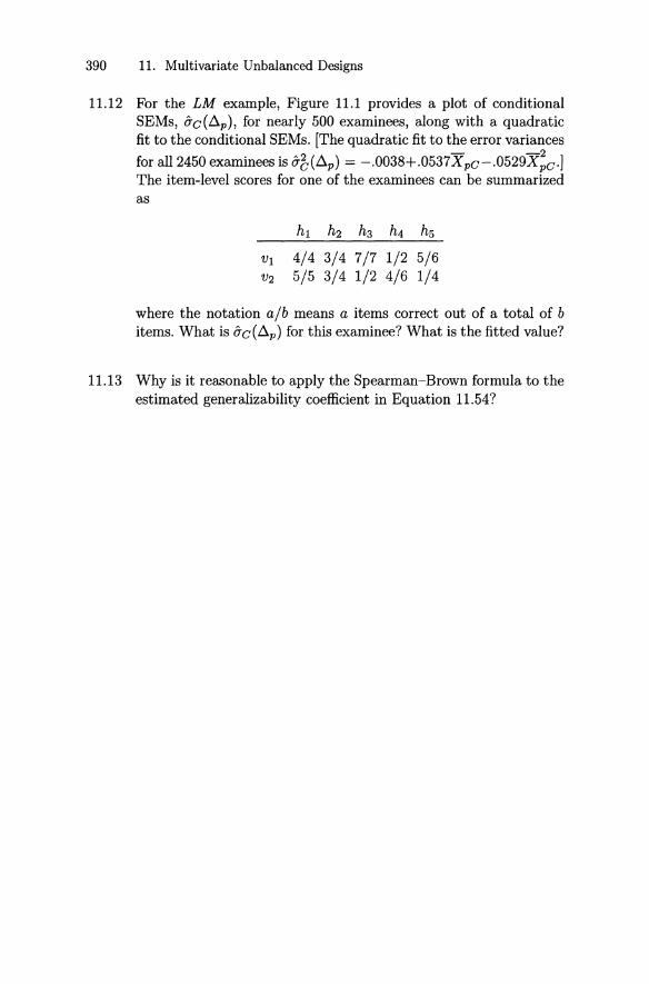
390 11. Multivariate Unbalanced Designs

11.12 For the LM example , Figure 11.1 provides a plot of conditionalSEMs, ac(~p), for nearly 500 examinees, along with a quadraticfit to the conditional SEMs. [The quadratic fit to the error variances

for all 2450 examinees is ab(~p) = -.0038+.0537Xpc-.0529X~c .]The item-level scores for one of the examinees can be summarizedas

VI 4/4 3/4 7/7 1/2 5/6V2 5/5 3/4 1/2 4/6 1/4

where the notation alb means a items correct out of a total of bitems. What is ac(~p) for this examinee? What is the fitted value?

11.13 Why is it reasonable to apply the Spearman-Brown formula to theestimated generalizability coefficient in Equation 11.54?

12Multivariate Regressed Scores

Recall from Section 5.5.2 that Kelley's regressed score estimates of truescore are easily extended to estimates of universe score in univariate gen­eralizability theory. The basic equation is

(12.1)

where p stands for an object of measurement. The principal way in whichunivariate generalizability theory extends Kelley's work is through themany different D study designs and universes of generalization that maybe employed to characterize E p2 and arrive at an estimate of it.

Multivariate generalizability theory permits us to extend furt her thesebasic ideas to the estimation of universe score profiles and universe scorecomposites. Kelley's original development was based on applying resultsfrom simple linear regression to the classical test theory model. We obtainregressed score estimates of profiles by applying results from multiple linearregression to models of the type used in generalizability theory. Doing sois relatively straightforward conceptually, but notational complexities caneasily obscure matters. For this reason, we begin with a review of basicresults for multiple linear regression with two independent variables usingrelatively standard terminology and notation. Then we translate these re­sults into the terminology of generalizability theory and the notation usedin this book. These developments permit us to obtain a multiple regressionestimate of each universe score. We call this set of estimates the estimateduniverse score profile.

After considering profiles, we show how the same basic multiple regres­sion theory can be used to obtain least squares estimates of composite

392 12. Multivariate Regressed Scores

universe scores. The theory applies to any composite universe score definedin terms of apriori weights. It is important to note that predictions of com­posite universe scores using multiple regression employ statistical weightsfor the observed scores, rather than the apriori (w) weights used to de­fine the composite. After discussing and illustrating the theory of predictedcomposites , relationships between predicted composites and estimated pro­files are considered.

In this chapter, the notation used does not explicitly distinguish be­tween parameters and estimates, with one important exception, namely, ahat A over a symbol designates a regressed score estimate. To maintain theparameter/estimate distinction everywhere would likely add more confu­sion than clarity to already complicated notational convent ions. Also, weoften use classical test theory notation when doing so results in simplerexpressions without limiting the generality of results. In addition, for sim­plicity, the discussion and notation assurne that the objects of measurementare persons , although the theory permits any facet to play that role.

Much of the discussion of profiles and predicted composites is in terms ofsingle-facet multivariate designs with n v = 2. The theory per se has no suchrestriction, however, and various parts of this chapter specify proceduresand equations for treating more complicated designs. One synthetic dataexample is used throughout to illustrate computat ions and discuss results.The results are hypothetical, of course, and not intended to be illustrativeof what is likely to happen with any particular real data set.

12.1 Multiple Linear Regression

The linear model for the regression of one dependent variable on two inde­pendent variables is

(12.2)

where(12.3)

Sometimes this is referred to as the raw score regression equation, to dis­tinguish it from the standard score regression equation:

(12.4)

where, for example, Zy = (Y - Y) / Sy with Sy designating the observedscore standard deviation for y. 1 The standard score regression equation is

1A mod el-fit error te rm e is included in both Equations 12.2 and 12.4, which is con­sistent with traditional statistical not ation. By cont rast , it is usual in measurement t exts

12.1 Multi ple Linear Regression 393

related to the raw score regression equat ion through the equalit ies

Syb1 = ßl -

SX l

and

(12.5)

Syb2 = ß2-

S' (12.6)

X2

where S X I and S X 2 are observed score standard deviat ions.The principal advantage of the standard score regression equation is that

the ßs have simpler expressions than the bs in the raw score regressionequat ion. The ßs can be obtained from the normal equations:

=(12.7)

where the TS are Pearson product-rnoment correlations. Using matrix pro­cedures it is relatively easy to determine that

and

ßTYX2 - TY X lTX I X2

2 = 21 - TX I X 2

Using Equ ations 12.5 and 12.6, it is easy to show that

b_ Syxtl s t - TXI X2 [SY X2/ ( SxI S x J l

1 - 21 - TX I X 2

(12.8)

(12.9)

(12.10)

and

(12.11)

(12.12)

The so-called multiple R2 is the squared correlat ion between Y and Y,which is the proportion of the variance in Y explained by the multipleregression. It can be shown that

R2 - ß ß _ blSYXI + b2SYX2- ITY X I + 2T y X 2 - S 2

Y

The st and ard deviation of dependent-variable observat ions about the re­gression line is called the standard error of est imate . For st andard scores itis

O'Zy lZx = VI- R 2, (12.13)

not to include t he e term in regressed score esti matio n equations such as Equation 12.1.This is not enti rely a matter of t radition, however. In Equ ati on 12.1, ind ividu al es arenot obse rvable because t he individual universe scores J.tp are not observable. Still, thetheory of regressed score esti mates implicitly recogn izes that es exist .

394 12. Multivariate Regressed Scores

or, letting [;z = Zy - Zy, it can be denoted aez . For raw scores, thestandard error of estimate is

aYIX = ay \.h - R2, (12.14)

or, let t ing [; = Y - Y, it can be denoted ae. The variance of the errorsof estimate for raw scores can be expressed in a number of different ways,including

2 2 2 2 2 2 (1 R2)ae=aYlx=a(y_y) =ay-ay=ay - .

Some of these equalities rely on the fact that a~ = ay y.T he extension to more than two independent variables , say k of them,

involves solving the normal equations

ßl + rx1x2ß2 + + rx1xkßk rYX1rX2x1ßl + ß2 + + rX2xkßk rYX2

(12.15)

rxkx1ßl + rXkx2ß2 + + ßk = rYXk'

Although the solutions of these equations are rather complicated expres­sions for the ßs, the basic notions and interpret at ions are unchanged fromwhat they are for the two-independent-variables case.

It is also possible, and sometimes easier, to obtain the bweights direct lyusing the variance-covariance matrix of observed scores. Specifically, thenormal equations for the bs are :

S11bl + SX 1x2b2 + + SX1Xk bk SYX1SX2X1b1 + St b2 + + SX 2xkbk SYX2

(12.16)

SXkx1b1 + SXkx2b2 + + Stbk SYXk '

where SX iXj is the observed score covariance for X, and Xj , and

These normal equations are often especially appealing in generalizabilitytheory because expressions for variances and covariances are usually simplerthan those for correlations. The ß weights for the standard score regressionare simply

SX ißi = bi Sy . (12.17)

A general formula for the variance of the predicted Y values is

k

S~ = I ) j S y x ;- (12.18)j=l

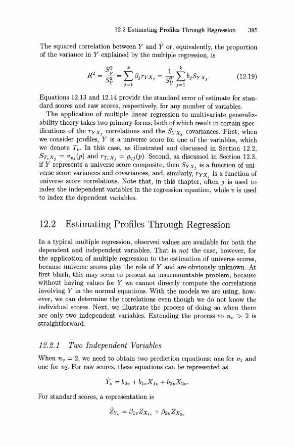
12.2 Estim ating Profiles Through Regression 395

The squared correlation between Y and Y or, equivalently, the proportionof the variance in Y explained by t he multiple regression, is

(12.19)

Equ ations 12.13 and 12.14 provide the standard error of est imate for st an­dard scores and raw scores, respectively, for any number of variables.

The application of multipl e linear regression to multivariat e generaliz­ability theory takes two primary forms, both of which result in certain spec­ifications of t he Tyx, correlatio ns and t he Syx, covariances. First , whenwe consider profiles, Y is a universe score for one of the variables, whichwe denote Tv . In t his case, as illustrat ed and discussed in Section 12.2,S Tv X ; = avj(p) and TTv X; = Pvj(p ). Second , as discussed in Section 12.3,if Y represents a universe score composite, then Syx , is a functi on of uni­verse score variances and covariances, and, similarly, TyX; is a function ofuniverse score correlations. Note t hat, in this chapter, often j is used toindex the independent variables in the regression equat ion, while v is usedto index the dependent variables.

12.2 Estimating Profiles Through Regression

In a ty pical multiple regression, observed values are available for both thedependent and independent variables. That is not the case, however, forthe application of mult iple regression to t he est imation of universe scores,because universe scores play the role of Y and are obviously unknown. Atfirst blush , this may seem to present an insurmountable problem, becausewithout having values for Y we cannot directly compute t he corre lationsinvolving Y in t he normal equations. With the models we are using, how­ever, we can determine the correlatio ns even t hough we do not know t heindividual scores. Next, we illustrat e t he process of doing so when thereare only two independent variables. Extending the process to n v > 2 isstraightforward.

12.2.1 Two Ind ependent Variables

Wh en nv = 2, we need to obtain two prediction equat ions: one for VI andone for V2. For raw scores, t hese equations can be represented as

Yv = bov + bIvXIv + b2vX2v.

For standard scores, a representation is

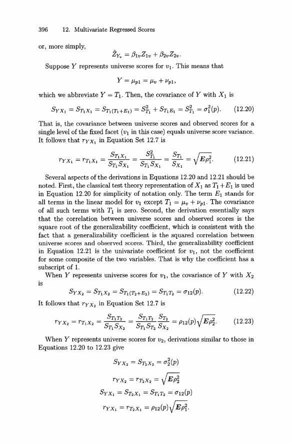
396 12. Multivariate Regressed Scores

or, more simply,ZYv = ßlvZlv + ß2vZ2v.

Suppose Y represents universe scores for VI. This means that

Y = J..Lpl = J..Lv + /lpl,

which we abbreviate Y = Tl . Then, the covariance of Y with Xl is

(12.20)

(12.21)

That is, the covariance between universe scores and observed scores for asingle level of the fixed facet (VI in this case) equals universe score variance .It follows that rYXI in Equation Set 12.7 is

_ _ Sn XI _ Sfl _ STI _ r;;:;,E2ry x I - rTIX I - S S - S S - -S - V J:J PI'

TI XI Tl XI XI

Several aspects of the derivations in Equations 12.20 and 12.21 should benoted. First , the classical test theory representation of X I as Tl +EI is usedin Equation 12.20 for simplicity of notation only. The term EI stands forall terms in the linear model for VI except Tl = J..Lv + /lpl' The covarianceof all such terms with Tl is zero. Second, the derivation essentially saysthat the correlation between universe scores and observed scores is thesquare root of the generalizability coefficient, which is consistent with thefact that a generalizability coefficient is the squared correlation betweenuniverse scores and observed scores. Third, the generalizability coefficientin Equation 12.21 is the univariate coefficient for VI, not the coefficientfor some composite of the two variables . That is why the coefficient has asubscript of 1.

When Y represents universe scores for VI , the covariance of Y with X2

isSYX2 = STIX2 = STI(T2+E2) = STIT2 = 0"12(p),

It follows that ry X2 in Equation Set 12.7 is

(12.22)

(12.23)

When Y represents universe scores for V2, derivations similar to those inEquations 12.20 to 12.23 give

SYX2 = ST2X2 = O"~(p)

rYX2 = rT2X2 = JEp~

SYXI = ST2XI = STIT2 = 0"12(P)

rYXI = rT2XI = PI2(P)JEPt·

12.2 Estimating Profiles Through Regression 397

Subsequently, to simplify notation, usually we use these abbreviationsfor observed score quantities:

(12.24)

Also, usually we abbreviate certain generalizability theory parameters as

P1 = JEPI, and PZ = JEp~. (12.25)

Note that we are using rand S for observed score statistics and P and (T

for the parameters of interest in the generalizability theory model.Using Equations 12.8 and 12.9, the beta coefficients for the standardized

regression of universe scores for V1 on observed scores for both variablesare

and (12.26)

Similarly, the beta coefficients for the standardized regression of universescores for Vz are

and (12.27)

These coefficients are relatively simple, but there is a subtle issue aboutthe definition of the generalizability coefficients in standardized regressions.For any level of v, the normal equations leading to the standardized re­gression coefficients involve standard scores for the independent (observed)variables and the dependent variable, that is, the universe scores for thelevel of v. This means that generalizability coefficients are not interpretableas ratios of variances for standardized universe scores and standardizedraw scores; such ratios are always unity. Rather, we must interpret gener­alizability coefficients as squared correlations between universe scores andobserved scores; such squared correlations are unaltered by the linear trans­formations involved in standardization.

Using Equations 12.10 and 12.11, the b coefficients for the raw scoreregression of universe scores for V1 on observed scores for both variablesare

and b = (Tl (PZP1Z - P1 r1Z) (1228)Z\T! S 1 Z ' •Z - r 1Z

with

bOIT! = Xl - b11T!X 1 - bZIT!XZ = (1- b11TJX 1 - bZIT!XZ. (12.29)

398 12. Multivariate Regressed Scores

Similarly, the b coefficients for the raw score regression of universe scoresfor V2 are

b _ 0"2 (PIPI 2 - P2r12)I1T2 - 8 1 r 2

1 - 12

with

and2

b - P2 - PIP2P12r12 (12.30)21T2 - 1 2 '- r12

(12.31)

Note that the observed score statistics can be expressed in terms of thegeneralizability theory model parameters as follows.

and

8 1 = J O"?(p) + 0"?(8) ,

82 = JO"~(p) + 0"~(8) ,

8 12 = 0"12(P) + 0"12(8) ,

(12.32)

(12.33)

(12.34)

(12.35)0"12 (p) + 0"12 (8)

r12 = -y'rO"=;;:r(7=p7=) =+=0"~r(if==8~)y"0"::::;~~(P:::::;)=+=0"=;~;=;:(8:::::=) '

It is particularly important to note that the observed covariance and cor­relation involve the correlated error component 0"12(8). When 0"12(8) f= 0,t he classical test theory formula for obtaining the disattenuated correlationfor the objects of measurement is not valid. In our abbreviated notationalsystem, when 0"12(8) =1= 0,

For expository purposes, let us focus, now, on the standardized regres­sions for the two universe scores. Using Equations 12.26 and 12.27, theregressed score estimate of the universe score profile is given by the follow­ing two equat ions.

(12.36)

(12.37)

where Zpvis to be understood in the sense of the Z score associated with thew edicted universe score for variable v (i.e., ZTvor, even more specifically,Z/-, pv), and Zpv is to be understood in the sense of the Z score associatedwith the vth raw score ZXpv' Using Equation 12.12, the proportions ofvariance explained by the two regressions are given by

(12.38)

12.2 Estimating Profiles Through Regression 399

and(12.39)

Using Equation 12.13, the corresponding standard errors of est imate areVI - Ri and VI - R~ , respect ively.

Regression to the Mean and Profile Flatness

Equ ations 12.36 and 12.37 const itute a regressed score est imate of the pro­file in two senses. First , both variables are regressed toward their respectivemeans (zero for t hese standardized regressions). This is guaranteed by thefact that R2 :::; 1 for both variables. In addit ion, the profile of predictedstandardized universe scores tends to be flatt er than t he profile of observedstandardized scores.

To illustrate these points, and to comment furth er on them, let us assumethat P1 = P2 in the standardized regression Equations 12.36 and 12.37.Under this assumption, using Equations 12.38 and 12.39,

R 2 _ R 2 _ R 2 _ 2 (1 + PI2 - 2P12T12)1 - 2 - -P 2'1 - T12

Clearly, R2 gets smaller as p2 decreases. Also, under classical test t heoryassumpt ions (or , equivalent ly, the p. x JO design), T12 = p2P12' and it canbe shown that R 2 gets smaller as !P12! decreases. Furthermore, for a con­stant positive value of P12 , R 2 gets smaller as T12 increases, which canoccur , for example, when there is positively correlat ed relative error (seeEquat ion 12.35) in the p. x J. design.

With P1 = P2 in Equations 12.36 and 12.37, it is easy to determine that

A A (1 -P12)Zp2 - Z p1 = P (Zp2 - Zp1 ).1 - T12

(12.40)

Whenever T12 :::; P12 , the coefficient of Zp2 - Z p1 is less than or equal tounity,2 which means th at

That is, the profile of predicted standardized universe scores tends to beflatter th an the profile of standardized observed scores.

These statements about regression to the mean and profile flatness areadmittedly complex, but the basic ideas apply to any number of variables,and to both standard and raw scores. These matters are discussed and

2Unde r classical test t heory assumptions, which correspond to th e ass um ptions fort he p. x JO design , Tl2 = PIP2PI2 , whic h necessarily mean s that Tl2 ::; P12. For t hep. x J. design , it is not necessarily true that Tl2 ::; P12, but it is very likely to be t ruewith real dat a .

400 12. Multivariate Regressed Scores

illustrated further in Sections 12.2.2 and especially 12.2.6. For now, wesimply note that the degree of regression to the mean and the flatness ofthe predicted profiles are affected by generalizability coefficients, universescore correlations, and the amount of correlated o-type correlated error;and all three factors influence the intercorrelations of the raw scores.

Extending the Theory

It is conceptually easy to extend the theory discussed thus far to obtain re­gression coefficients, R2 values, and standard errors of estimate for nv > 2,for both standard scores and raw scores, but the algebra is more compli­cated. The crux of the matter is to determine the normal equations (Equa­tion 12.15 for standard scores, or Equation 12.16 for raw scores), and thensolve them for the regression weights . For raw scores, the left side of thenormal equations involves the observed score variances and covariances forall nv variables. For variable v, the right side involves the covariances

(12.41)

Using these covariances in Equation 12.19, along with the derived b weightsgives

R2 a~(p,p)(12.42)v ----;;:2v

Lj bjvavj(12.43)

a2v

With S~ = a~ in Equation 12.14, the associated standard error of estimateis:

(12.44)

For standard scores, the left side of the normal equations involves theobserved score correlations for all nv variables. For variable v, the rightside involves the correlations

{Pv if v = j

TYXj = TTvXj = PvjPj if v i= j. (12.45)

Using these correlations in Equation 12.19 along with the derived ß weights,gives R~ . The associated standard error of estimate ave&) is given by Equa­tion 12.13.

Profile equations and their associated statistics [e.g., R2 and ace)] areD study results. We have discussed estimating them primarily under theassumptions that the G and D study sampie sizes are the same, and theD study design structure mirrors that used in the G study (e.g., p. xi·and p. x J., or p. x iO and p. x JO

) . It is possible, however, to estimateprofile equations for sampie sizes and/or designs different from those used

12.2 Estimating Profiles Through Regression 401

in a G study. That is, we can obtain answers to "What if . . . " questionsfor regressed score estimates of profiles, just as we can for other D studystatistics. To do so, the normal equations must be specified for the D st udysam pie sizes and design . For example, for raw score profile equations, in­stead of using the observed variances and covariances from the G study,the investigator would use their expected values for th e D study sam plesizes and design . Für any particular level of v , th e right side of the nor­mal equat ions is unchanged, because the right side involves only universescore variances or covariances. This process is illustrated at the end ofSection 12.2.2 and then again in Sect ion 12.2.5.

12.2.2 Synthetic Data Example

Consider the synthetic data example for the p. x i· design in Table 9.3for 10 persons, six items, and two fixed variables, in which each item con­tributes scores for each variab le. Assuming n~ = ni = 6, the reader caneasily verify that

~p [ .3682 .8663 ] (12.46).3193 .3689

~o [ .2087 .5081 ] (12.47).1175 .2561

S [ .5769 .7273 ] (12.48)= .6250 '.4367

where the entries in italics in th e upper-diagonal cells are correlations.Note in particular that th e observed score correlation T12 = .7273 is notequal to th e universe score correlat ion PI2 = .8663, because of the 8-typecorre lated-error component aI2(J) = .1175 (see Equati on 12.35). Also, it iseasily verified that

2 = .3682 = .6382PI .5769

and2 .3689

P2 = .6250 = .5902. (12.49)

Using these result s in Equat ions 12.36 and 12.37 gives th e regressed scoreest imates of the Z-score profile equat ions:

Zpl .6684 Z pl + .1794 Zp2

Zp2 .2830 Zpl + .5624 Z p2

andZp2 - Zpl = .3830 Zp2 - .3853 Z pl .

This suggests that th e predicted profile is about 38% flatter than the ob­served profile.

402 12. Multivariate Regressed Scores

TABLE 12.1. Regressed Score Estimates for Synthetic Data Example for Bal­anced p. x r Design in Table 9.3

Standard Scores Regressecl-Score Estimates

p Zpl Zp2 Mean Var" Zpl Zp2 Mean Var''

1 -.2544 - .1111 - .1828 .0051 -.1900 -.1345 - .1623 .00082 -1.4110 - .5556 - .9833 .1829 -1.0427 - .7118 -.8773 .02743 .6708 -.3333 .1687 .2521 .3885 .0024 .1955 .03734 -1.8736 -1.6667 -1.7701 .0107 -1.5513 -1.4676 -1.5095 .00185 -.2544 - .7778 -.5161 .0685 -.3096 - .5094 -.4095 .01006 1.3647 2.1111 1.7379 .1393 1.2910 1.5736 1.4323 .02007 .4395 .1111 .2753 .0270 .3137 .1869 .2503 .00408 - .0231 1.2222 .5996 .3877 .2039 .6808 .4423 .05699 1.3647 .3333 .8490 .2660 .9720 .5737 .7728 .0396

10 - .0231 -.3333 -.1782 .0241 - .0753 - .1940 - .1346 .0035

Mean .0000 .0000 .0000 .1363 .0000 .0000 .0000 .0201Vara 1.0000 1.0000 .8637 .0158 .6534 .6280 .6205 .0003

Zpl = .6684 Zpl + .1794 Zp2 Ri = .6534

Zp2 = .2830 Zpl + .5624 Zp2 R~ = .6280

Raw Scores Regressed-Score Estimates

p X p1 X p2 Mean Vara{lpl {lp2 Mean Vara

1 4.3333 5.0000 4.6667 .1111 4.4073 5.0058 4.7066 .08962 3.5000 4.6667 4.0833 .3403 3.9165 4.6732 4.2948 .14323 5.0000 4.8333 4.9167 .0069 4.7403 5.0847 4.9125 .02974 3.1667 3.8333 3.5000 .1111 3.6237 4.2377 3.9307 .09435 4.3333 4.5000 4.4167 .0069 4.3384 4.7898 4.5641 .05096 5.5000 6.6667 6.0833 .3403 5.2598 5.9900 5.6249 .13337 4.8333 5.1667 5.0000 .0278 4.6972 5.1910 4.9441 .06108 4.5000 6.0000 5.2500 .5625 4.6340 5.4756 5.0548 .17719 5.5000 5.3333 5.4167 .0069 5.0761 5.4139 5.2450 .0285

10 4.5000 4.8333 4.6667 .0278 4.4733 4.9716 4.7224 .0621

Mean 4.5167 5.0833 4.8000 .1542 4.5167 5.0833 4.8000 .0870Vara .5192 .5625 .4669 .0337 .2165 .2085 .2058 .0023

{lpl = 1.4050 + .5339 X p 1 + .1377 X p2

{lp2 = 1.8647 + .2263 X p1 + .4321 X p2

aBiased estimates.

0'1 (E) = .3572

0'2(E) = .3705

12.2 Estimating Profiles Through Regression 403

The top half of Table 12.1 provides the observed Z-scores and regressedscore estimates for each of the 10 persons .i' Also provided are means andvariances for all variables. For both VI and Vz, regression to the mean occursin the sense that the variance of the regressed score estimates is smaller thanthe variance of the standardized universe scores. This fact is evident fromthe results reported in Table 12.1. For example , for VI , the variance of Zplis .6534, and the variance of the standardized universe scores is necessarilyone. Since RZ is the proportion of universe score variance explained by theregression , it follows that Rr = .6534. Alternatively, Rr can be obtainedusing Equations 12.12, 12.21, and 12.23:

Ri ßITyX, + ßzTY X2

ß IPI + ßZPIZPZ

= .6684\1".6382 + .1794(.8663)\1".5902

.6534.

The top half of Table 12.1 also illustrates that regression occurs in thesense that the profiles of predicted standardized universe scores are usu­ally flatter than the profiles of observed standardized scores. Specifically,the average within-person variance for the regressed standardized scores(.0201) is less than the average within-person variance for the observedstandardized scores (.1363), which means that the regressed standardizedscores are about 85% less variable than the observed standardized scores.

For this synthetic data example , the bottom half of Table 12.1 providesresults in the raw score metric. Using Equations 12.28 to 12.31, the profileequations are

Ppl 1.4050 + .5339 X p l + .1377 X p2

[lp2 1.8647 + .2263 X p l + .4321 X pz .

Alternatively, bl and b: for VI can be obt ained by solving the normal equa­tions

.5769bl

.4367bl

+ .4367bz+ .6250bz

.3682.3193,

(12.50)

with bo determined using Equation 12.29. Similarly, bl and bz for Vz canbe obtained by solving the normal equations

.5769bl

.4367bl

+ .4367bz+ .6250bz

.3193.3689,

(12.51)

with bo determined using Equation 12.31.

3T he observed Z scores were computed using the so-called "biased" variances (Le.,using adenominator of 10) . Also, all within-person variances are "biased." That is, inTable 12.1 "Var" indicates "biased" variances.

404 12. Multivariate Regressed Scores

The R 2 values are necessarily the same for raw scores as they are forstandard scores, because the two types of scores are linear transformationsof each other. It follows that, for Vl, the proportion of universe score vari­ance explained by the regression is R~ = .6534. This value can also beobtained using Equation 12.42:

R2 = (TI({Lp) = .2404 = .65341 (TI .3682 '

where (TI = .3682 is provided in Equation 12.46, and (TI({Lp) = .2404 isthe "unbiased" version of the variance (.2165) reported at the bottom ofTable 12.1. Using Equation 12.44, the standard error of estimate for Vl is

(Tl(&) = (Tl VI - R~ = ).3682)1 - .6534 = .3572.

R2 = (T~({Lp) = .2317 = .62802 (T~ .3689 '

and the standard error of estimate is

Similarly, for V2, the proportion of universe score variance explained by theregression is

It is also evident from the bottom half ofTable 12.1 that regression occursin the sense that the profiles of predicted universe scores are generally flatterthan the profiles of observed (raw) scores. Specifically, the average within­person variance for the regressed scores (.0870) is less than the averagewithin-person variance for the observed scores (.1542), which means thatthe regressed scores are about 44% less variable than the observed scores.

12.2.3 Variances and Covariances of Regressed Scores

Table 12.2 provides formulas for variances and covariances of regressedscore estimates for any number of variables. Although the formulas arequite general, many of them are rather unusual compared to traditionalregression results. For this reason , some of them are explained here.

Formulas for variances and covariances are reported in several ways. Foreach such formula, the first expression is in terms of n~ sums of productsof ß weights and observed correlations (for standard scores) , or n~ sumsof products of b weights and observed variances and covariances (for rawscores). These are "t radit ional" expressions from multiple regression theory,although they are usually st ated in matrix terms. Because they involve n;sums of products , they are tedious to compute.

The remaining expressions for variances and covariances have only nvproducts, each of which involves a universe score correlation (for standard

12.2 Estimating Profiles Through Regression 405

TABLE 12.2. Formulas for Multivariate Regr essed Score Estimates of UniverseScores

Standard Scores

Rvv

' = r7vv' (Zp)

Pvv'

r7~(Zp) = L L ßjvßj'vrjj' = L ßjvPjPVj = R~j= l j' =l j=l

n v n v n v n v

r7vv'(Zp) = L L ßjvßj' v,r jj' = Lßjv'PjPVj = L ßjvP jPV'jj=l j'=l j=l j=l

V(ZX p ) = 1 - rvv'

V(ZJLp) = 1 - avv'

A - 2 A -2-V(ZJLp) = R v - a vv'(Zp) = R v - R vv'

Raw Scores

n v nv n v

r7~(fi,p) = L L bjvbj' vSjj' = L bjvr7vj = R~r7~j=l j'=l j=l

n v n v n v n v

r7vv'(fi,p) = L L bjvbj' v,Sjj' = L bjv'r7vj = Lbjvr7v' jj=l j '= l j=l j=l

- np -1 - 2 - -V(Xp) = --[Sv - Svv'] + var(X v )

n p

n -1 2V(JL p) = -P--[av - O'vv'] + var(Mv)

np

V({.tp) = np

- 1 [a~(fi,p) - avv'(fi,p)] + var(fi,v)np

Not e. bjv is an abbreviat ion for bj lTv or, even more specifically, bil JL pv ' 8imilarly, ß j v

is an abbreviatio n for ßj lTv' The notations ä'v v ' , S vv" and Rv v ' mean th e average over2 2 - 2 d - 2 h f h Iall nv elements; ä'v ' Sv, an R v mean t e average 0 t e squares over nv e ements.

406 12. Multivariate Regressed Scores

scores), or a universe score variance or covariance (for raw scores). Thesesimplified expressions do not apply in multiple regression generally. Rather,they are a consequence of the fact that, for regressed score estimates, thedependent variable is the universe score for one of the independent vari­ables. A unique and useful feature of these expressions is that they dependonly on the regression weights and the elements of :Ep .

Consider, for example , the formula for the variance of the regressed scoreestimates for v:

n v

<7;(flp) = I>jv<7vj. (12.52)j=1

Note that bjv is an abbreviation for bjlTv or, even more specifically, bjl/Lpv 'Applied to the synthetic data example for VI, this equation gives

<7r(flp) = bll <711 + b21<7I2 = .5339(.3682) + .1377(.3193) = .2405, (12.53)

which is the unbiased version of the result reported at the bottom of Ta­ble 12.14 ; that is, (10/9) x .2405 = .2165. Essentially, then, <7r(flp) is thesum of the products of the b terms and <7 terms for VI. For V2 , the varianceof raw score regressed score estimates is

<7~(flp) = b12<72I + b22<722 = .2263( .3193) + .4321(.3689) = .2316, (12.54)

which is the sum of the products of the b terms and <7 terms for V2 .There are two simplified formulas for the covariance of the regressed score

estimates:n v n tJ

<7vv,(flp) = I~)jvl<7Vj = I)jv<7v'j . (12.55)j=l j=1

That is, <7vv' (flp) is the sum of the products of the b terms for Vi and the<7 terms for vor, equivalently, the sum of the products of the b terms for V

and the <7 terms for o', For the synthetic data, using the first formula,

<712(flp) = b12<711 + b22<7I2 = .2263(.3682) + .4321(.3193) = .2213, (12.56)

and using the second formula,

<7I2(flp) = bll <721 + b21<722 = .5339(.3193) + .1377( .3689) = .2213.

It follows that the estimated correlation between regressed score estimatesfor VI and V2 is

.2213~ !"'AA1i5 = .937.

y .2405y .2316

4For the purposes of the discussion here, obviously it would be better to repo rtthe unbiased estimates in Table 12.1. However, for the subsequent discussion of profilevariability, the so-called "biased" estimates are more convenient . In any case, with datasets of typical size, this is a trivial matter.

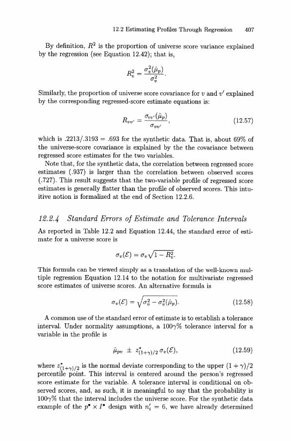
12.2 Estim ating Profiles Through Regression 407

By definition, R2 is the proportion of universe score variance explainedby the regression (see Equation 12.42); that is,

Similarly, t he proportion of universe score covariance for v and v' explainedby the corresponding regressed-score est imate equations is:

u.; = (lvv'(/lp) ,

(lvv'(12.57)

which is .2213;'3193 = .693 for the synthetic dat a. Th at is, about 69% ofthe universe-score covariance is explained by the the covariance betweenregressed score estimates for the two variables.

Note that , for the synthet ic dat a, the correlation between regressed scoreest imates (.937) is larger th an the correlat ion between observed scores(.727). This result suggests that the two-variable profile of regressed scoreest imates is generally flatter than the profile of observed scores. This intu­itive not ion is formalized at the end of Section 12.2.6.

12.2.4 Standard Errors of Estimate and Tolerance Intervals

As reported in Tab le 12.2 and Equation 12.44, the standard error of est i­mate for a universe score is

This formula can be viewed sim ply as a trans lation of t he well-known mul­t iple regression Equat ion 12.14 to the notation for multivariate regressedscore est imates of universe scores. An alternative formula is

(12.58)

A common use of the standard error of est imate is to establish a toleranceinterval. Under normality assumpt ions, a 100''{% toleran ce interval for avariable in th e profile is

(12.59)

where z(1+oy)/2 is the normal deviate corresponding to the upper (1 + "{) /2percentile point. This interval is centered around the person's regressedscore est imate for the variable. A tolerance interval is condit ional on ob­served scores, and, as such, it is meaningful to say that the probability is100"{% t hat the interval includes the universe score. For the synthetic dataexample of the p. x J. design with n~ = 6, we have already dete rmined

408 12. Multivariate Regressed Scores

in Section 12.2.2 that 0"1 (E) = .3572 and 0"2(E) = .3705. Und er normal­ity assumpt ions, it follows that 68% tolerance intervals for V I and V2 arePpl ± .3572 and Pp2 ± .3705, respect ively.

As reported in Table 12.2, the covariance of the errors of est imate is

(12.60)

An alternative formula is

(12.61)

For the synthetic data example of the p. x J. design with n~ = 6,

(.2213)0"12(E) = .3193 1 - .3193 = .3193 - .2213 = .0980.

Since the standard errors of estimate for the two variables are .3572 and.3705, the correlation between the errors of estimates for the two variablesis

.0980PI2(E) = .3572 x .3705 = .740.

The covariance between correlated E-type errors, O"vv,(E), plays an im­portant role in making probability statements ab out overlapping toleranceintervals for universe scores . For example, under normality assumptions,the probability that 100,% tolerance intervals for v and v' will overlapwhen /Lpv = /Lpv' is

{Z(l+ )/2 [O"v(E) + O"v,(E)] }

Pr(overlap) = 2 x Pr z < 'Y - 1,JO"~(E) + O"~,(E) - 20"vv,(E)

(12.62)

provided, of course, that the intervals are formed in the multivariate mannerdiscussed in this chapter.f The logic leading to Equation 12.62 mirrors thatdiscussed in Section 10.2.4 for confidence intervals.

For the synthetic data example of the p. x r design with n~ = 6, using68% tolerance intervals,

Pr(overlap) 2 P{

.3572 + .3705 }= x r z < -1J(.3572)2 + (.3705)2 - 2(.0980)

= 2 x Pr(z < 2.7727) - 1

2(.9972) - 1

= .994,

5Equation 12.62 would not apply if the two tolerance int ervals were obtained usingthe univariate Equation 12.1.

12.2 Estimating Profiles Through Regression 409

which means it is virtually certain that two 68% tolerance intervals willoverlap when J..lpv = J..lpv" This probability-of-overlap result is conditionalon the D study p. x I" design with n~ = 6 for both variables. If the designand/or sample sizes change, then the standard errors of estimate and thecovariance of the errors of estimate will change (see Table 12.3 for a num­ber of examples). Note , in particular, that it is not necessarily true thateTvv' (&) = 0 for the p. x JO design, even though eTvv' (8) = 0 for this design.

If tolerance intervals are constructed for an examinee's scores on differenttests in a battery, then a relative strength or weakness for the examineemight be declared if the intervals for two test scores do not overlap. This isthe same kind of logic discussed in Section 10.2.4 for confidence intervals.For any specific confidence coefficient, tolerance intervals will be shorterthan confidence intervals, because the standard error of estimate is smallerthan the standard error of measurement. This may appear to suggest thatthere is likely to be a greater probability that a relative strength or weaknesswill be declared using tolerance intervals than using confidence intervals .Actually, however, matters are more complicated than this ad hoc rea­soning suggests , because tolerance intervals are centered around regressedscore estimates of universe scores, whereas confidence intervals are centeredaround observed mean scores.

Recall from Section 10.2.4 that for the synthetic data example of thep. x I" design with n~ = 6, using 68% confidence intervals, the probabil­ity of overlap was .946. By contrast, in this section we obtained .994 fortolerance intervals . This means that a relative strength or weakness is lesslikely to be declared using tolerance intervals in this example.

12.2,5 Different Sample Sizes tuui/or Designs

Profile equations are D study results . In univariate generalizability theory,it is a relatively simple matter to estimate results for a D study that hasa different set of sample sizes and/or design structure from that used ina G study. This can be done for profiles, too, but the process is not assimple. The most general approach is to state the normal equations for therevised design, solve them for the regression coefficients, and then use theequations in Table 12.2 to obtain the desired results. Of course, if n v = 2,solving the normal equations can be circumvented by using the equationsin Section 12.2.1 directly.

It is important to realize that the D study design and sample sizes af­fect observed score variances and covariances and, of course, any quantitiesbased on them. Since observed score variances and covariances are incor­porated in the left side of the normal equations, regression weights areaffected by changes in design and/or sample sizes , Universe score variancesand covariances are not affected.

Let us now reconsider the synthetic data example for the p. x J. designusing n~ = 8 rather than n~ = 6. Statistics that are sample-size dependent

410 12. Multivariate Regressed Scores

are altered. For vI ,

Sr = .3682 + .1565 = .5247,

2 = .3682 = .7017PI .5247 '

2 1.53670"2(8) = -8- = .1921,

si = .3689 + .1921 = .5610,

and 2 = .3689 = .6576.P2 .5610

Also, using Equation 12.34, the expected observed covariance (l.e., the valueof the observed covariance that is expected for n~ = 8) becomes

.7048S12 = 0"12(p) + 0"12(8) = .3193 + -8- = .4074,

and using Equation 12.35 the corresponding observed correlation is

T12 = .4074

= .7508.V.5247V.561O

The normal equations are

.5247b 1 + .4074b2

.4074b1 + .5610b2 =.3682.3193.

(12.63)

These equations can be solved for the bs or, more simply, we can use theclosed-form expressions in Equation 12.28. Note that these normal equa­tions involve smaller observed score variances and covariances than thosein Equation 12.50 for n~ = 6.

The resulting regressed score estimation equation for VI is

{lpl = 1.1321 + .5956Xp1 + .1366 X p2 .

It follows that

R2 = .5956(.3682) + .1366(.3193) =1 .3682 .7141

and the standard error of estimate is

O"I(E) = V.3682V1 - .7141 = .3244.

Now, suppose both the design and sample size are different from thatused in the G study. Specifically, suppose the design is p. x J O with n~ = 8for both variables. For this design, there is no correlated o-type or Do-typeerror. All the statistics are the same as for the p. x r design with n~ = 8except for S12 and T12 . Since 0"12(8) = 0, Equations 12.34 and 12.35 give

S12 = 0"12(p) = .3193 and T12 = .3193 = .5885.V.5247V.5610

12.2 Estimating Profiles Through Regression 411

TABLE 12.3. Changes in RZ, Standard Errors of Estimate, and Other Statistics

for Different Sample Sizes and Designs with the Synthetic Data in Table 9.3

Design v n~ p2 b1 b2 R2 O"(E) R12 0"12 (E) V(iJ,p) r12

p. x J. 1 6 .6382 .5339 .1377 .6534 .35722 6 .5902 .2263 .4321 .6280 .3705 .6931 .0980 .0870 .7274

p. x t: 1 8 .7017 .5956 .1366 .7141 .32442 8 .6576 .2245 .4946 .6889 .3388 .7535 .0787 .0884 .7509

p. x JO 1 6 .6382 .4956 .2577 .7190 .32162 6 .5902 .3162 .4287 .7024 .3314 .7933 .0660 .0842 .5317

p. x JO 1 8 .7017 .5436 .2597 .7689 .29172 8 .6576 .3187 .4762 .7520 .3024 .8437 .0499 .0852 .5885

J. :p. 1 6 .5804 .4666 .1597 .6051 .38132 6 .5438 .2205 .3969 .5877 .3900 .6511 .1114 .0856 .6892

r:p· 1 8 .6485 .5280 .1632 .6696 .34882 8 .6138 .2254 .4568 .6518 .3584 .7166 .0905 .0869 .7171

JC :p. 1 6 .5804 .4502 .2588 .6746 .34612 6 .5438 .3009 .4022 .6626 .3528 .7492 .0801 .0835 .4867

JO :p. 1 8 .6485 .4987 .2663 .7296 .31552 8 .6138 .3097 .4493 .7173 .3229 .8064 .0618 .0844 .5466

Note. Für VI , bo = (1 - bd(4.5167) + bz(5.0833) jfür Vz , bo = (1 - bz)(5.0833) + bi (4.5167) .

The resulting regressed score estimation equation for VI is

PpI = .7410 + .5436 X pI + .2597 X p2 ,

which leads to Rr = .7689 and 0"1 (E) = .2917.The top half of Table 12.3 summarizes the results for both crossed-design

structures (p. x rand p. x JO), both sampie sizes (n~ = 6 and n~ = 8),and both variables. Note that , for both variables, R2 increases and O"(E)decreases when :

• the design stays the same (p. x r) , but sarnple size (nD increases,leading to larger generalizability coefficients; or

• sampie size stays the same, but the design changes from one withlinked conditions (p. x r) and positively correlated <>-type errors tothe corresponding design with uncorrelated <>-type errors (p. x JO).

These conclusions generalize to other sample sizes and designs. See, forexample, the results in Table 12.3 for the J. :p. and JO :p. nested designs.

Note that positively correlated <>-type error leads to larger raw scoreintercorrelations (rI2) for the p. x I" design. Therefore, larger raw score

412 12. Multivariate Regressed Scores

intercorrelations that result from joint sampling, as opposed to independentsampling, are associated with smaller values for R2 and larger standarderrors of estimate for individual universe scores."

As indicated by the results in Table 12.3, Rvv' and O"vv,(E) are also af­fected by changes in the D study design structure and/or sample sizes.Consider, for example, the p. x [0 design with n~ = 6. The normal equa­tions are the same as those in Equation 12.50 except that the covariance.4367 is replaced by .3193:

.5769bl

.3193bl

+ .3193b2

+ .6250b2

.3682.3193.

Solving these equations for the regression coefficients gives

bi = .4956

Using Equation 12.55

and bz = .2577.

O"l2(flp) = (.4956)( .3193) + (.2577)( .3689) = .2533,

which leads to

Note , in particular, that O"vv' (E) is not zero for the p. x [0 design withn~ = 6, although it is smaller than O"vv'(e) = .0980 for the p. x I" design.

12.2.6 Expected Within-Person Profile Variability

When profiles are under consideration, usually interest focuses on individ­ual persons, as discussed in Sections 10.2.4 and 12.2.4 . To characterize theentire measurement procedure for a population, however, we can considerexpected within-person profile variability using the V(*) formulas in Ta­ble 12.2. For both standard and raw scores, three formulas are provided­one for observed scores, one for universe scores, and one for regressed scoreestimates of universe scores. The logic behind the derivation of these formu­las was developed in Section 10.2.5 (see especially Equation 10.55) , whichalso discussed V(Xp ) and V(J.Lp ) '

The expected regressed score profile variability is

(12.64)

6In the context of the discussion here , changes in raw score intercorrelations are aconsequence of cha nges in the amount of 8-type correlated error, not changes in universescore covariances or correlations.

12.2 Estimating Profiles Through Regression 413

We take this equation as adefinition of expected profile fiatness or, morespecifically, lack of fiatness. For the synthetic data with n~ = 6 for thep. x j. design, the computational results in Equations 12.53, 12.54, and12.56 give

V(jLp) = .9(.2361 - .2287) + .0803 = .0870.

This is the value reported in Table 12.1 based on direct computation of theaverage (over persons) of the variances of the regressed score estimates.?

The fiatness of the profiles of predicted scores is affected by generalizabil­ity coefficients, universe score correlations, and <>-type correlated errors-allthree of which affect raw score intercorrelations. In general ,

• larger generalizability coefficients,

• larger values of Ip121 , and

• decreases in <>-type correlated error

tend to be associated with less regression to the mean , smaller standarderrors of estimate, and fiatter profiles of predicted scores. The reader canverify that these statements are consistent with results reported in Ta­ble 12.3 for the synthetic data.

Using the formulas in Table 12.2, it can be shown that

which mirrors the inequality relationships in univariate theory"; that is,

As in univariate theory, it is natural to consider various functions of vari­abilities, particularly ratios. One such ratio is given by Equation 10.60 inSection 10.2.5:

V(J.Lp )

9 = V(Xp

) ,

which is interpretable approximately as a type of generalizability coefficientfor a randomly selected person p.

Another obvious ratio to consider is

(12.65)

7For this example, uvv,({i.p) is the average over four terms, not two. Also, var({i.v) isthe biased estimate of the variance of the two means (4.5167 and 5.0833) .

8(T2(Xp) is the variance of observed persons' mean scores for the population, whichwas denoted ES2 (p) in earlier chapters.

414 12. Multivariate Regressed Scores

which we designate n2 because of its obvious similarity to the squaredcorrelation in a multiple regression." This ratio can be interpreted approx­imately as the proportion of expected variability in universe scores for a"typical" person that is explained by the regressions. For the syntheticdata with n~ = 6 for the p. x r design, n2 = .0870;'1024 = .849. Thecorresponding approximation to the variance of the errors of estimate fora typical person is

(12.66)

(12.67)

which is .015 for the synthetic data. This means that the standard error ofthe regressed score estimates for a typical person is roughly ).015 = .12.Recall that the standard deviation of the 8-type errors of measurement fora typical person is ).058 = .24, which is twice as large as the standarderror of estimate. Such statements are sometimes used as an argument infavor of using regressed score estimates.

Finally, the proportional reduction in profile variability attributable tousing regressed score estimates is

nv = 1 _ V(jJ,p)V(Xp),

which is 1 - .0870;'1542 = .436 for the synthetic data with n~ = 6 forthe p. x I" design. That is, for a typical person, the use of regressed scoreestimates reduces profile variability by about 44%. This particular value canbe computed directly (although less efficiently) using the persons' scoresin Table 12.1, whereas 9 and R 2 cannot, since universe scores for anyparticular person are unknown.

Also, direct computation ofnV (and its component parts) is not possiblefor different sample sizes and/or designs, because , of course, persons' ob­served scores are unavailable for different sample sizes and/or designs. Theformulas in Table 12.2 can be used, however. For example, for the p. x JO

design with n~ = 6, these formulas give V(Xp) = .2070 and V(jJ,p) = .0842,which leads to nv = .593. Comparing this result to nv = .436 for thep. x J. design, it is evident that, for a typical person , the use of the p. x JO

design leads to greater reduction in profile variability (i.e., a flatter profile)than does the p. x I" design.

Although measures of relative variability for profiles have conceptualsimilarities with traditional statistics in univariate generalizability theory,there are differences, too. In particular, in univariate theory with a singledependent variable,

9p reviously, n was used to designate a set of randorn facets . Obviously, n 2 is notthe square of a set of randorn facets .

12.3 Predicted Composites 415

but the corresponding equality does not hold for the relative variabilityindices based on multiple dependent variables; that is,

12.3 Predicted Composites

The multiple linear regression procedure described in Section 12.1 can beapplied also to composites of k = nv universe scores. For example, theprediction equation for raw scores is

(12.68)

and there is a corresponding equation for standard scores in terms ofß weights. It is important to recognize that the left-hand side of Equa­tion 12.68 is an estimate of

y = fJ.pc = Wl fJ.pl + ... + Wk fJ.pk· (12.69)

Since both the left- and right-hand sides of Equation 12.68 are linear com­posites, the equation is reminiscent of a canonical correlation, but there is avery important difference. Namely, the left-hand side is a composite basedon apriori (i.e., investigator-specified) weights, and only the right-hand sideis based on statistically optimal (in a least-squares sense) weights. (For acanonical correlation, both sides are based on statistical weights.)

To estimate the b weights in Equation 12.68 , the crux of the matter isto express the right side of the normal equations (Equation 12.16) withrespect to estimable model parameters. Once that is done, the equationscan be solved for the b weights. When the independent variables (X pv)are observed score versions of the same variables that enter the composite(fJ.pv) , the right-hand sides of the normal equations are the covariances

n v

SYX j = L wvavj,v=l

(12.70)

where Y = fJ.pc, avj = avj(p) in the simplified notation introduced inEquation 12.25, and j indexes the observed scores for the nv variables .

Replacing Equation 12.70 in Equation 12.18 gives the following formulafor the variance of the regressed score estimates of the composite,

(12.71)

416 12. Multivariate Regressed Scores

It follows that R2 for the predicted composite scores is

R~CJ~(fLp)

CJ~(J.Lp)

L::j bj (L::v wvCJvj)

L::j Wj (L::v wvCJv j) '

(12.72)

(12.73)

where all summations range from 1 to nv .

With error defined as Epc = J.L pc - jlpc , the standard error of est imateis

=

CJc(E) = CJc(J.Lp)V1 - R~

~(Wj -bj)(~w"a"j),

(12.74)

(12.75)

where, again, both summations range from 1 to nv . Under normality as­sumptions, a two-sided 1001% tolerance interval for universe compositescores is

jlpc ± Z(1+"Y)/2 CJc(E) , (12.76)

where Z(1+"Y )/ 2 is the [100(1 +1)/2]th percentile point of the normal dis­tribution. The tolerance interval is centered around the regressed score es­timate of the composite score. Such an interval is condit ional on observedscores and , as such, it is meaningful to say that the true composite scoreis contained within the interval 1001% of the time.

As indicated by Equation 12.73, R~ is interpretable as the proportionof universe composite scores predicted by the regression. Equivalently, R~is the squared correlat ion between universe composite scores and predictedcomposite scores. As such, Rb is a type of reliability or generalizabilitycoefficient .

Both Rb in Equat ion 12.73 and CJc(E) in Equation 12.75 are expressedin terms of b weights, W weights, and elements of ~p . No other parame­ters or statistics are required , although there are equivalent expressions forRb and CJc(E) that make it app ear that other parameters and statisticsare involved. Error variances associated with the individu al var iables areabsorbed into these equat ions th rough the b weights.R~ and CJc(E) apply for any universe score composite, even t riviai ones.

For example, the formulas for R~ and CJv(E) for profiles (see Table 12.2)are special cases of these two equations in which W v = 1 and the other wsare zero.

The theory outlined above for predicted composites is illustrated next byconsidering difference scores. This is th e simplest example of a multivariatepredicted composite in that it requires considering only nv = 2 variables,which permits us to make direct use of the result s in Section 12.1 that

12.3 Predicted Composites 417

introduced multiple linear regression. Consequently, we can examine alge­braic expressions for the b weights, which is not easily done when nv > 2.This generalizability theory perspective on difference scores is considerablymore flexible than trad it ional perspect ives.

12.3.1 Difference Scores

When there are two independent variables, an obvious example of a compos­ite is difference, change, or growth scores. In our notation, t his compositeis J.L pc = J.Lp2 - J.Lpl , which means that W2 = 1, and Wl = -1. We wish toobtain th e prediction equation

To do so we use Equati ons 12.10 and 12.11.In classical test theory notat ion, th e universe score composite is typic ally

denoted Y = T2 - Tl . T he covariance of universe difference scores with Xlis

S Y X 1 = S(T2-TJl(T1+EJl = ST1T2 - Sj,1 = a12 - af.Similarly, t he covariance of universe difference scores with X2 is

(12.77)

(12.78)

Replacing these results in Equations 12.10 and 12.11 gives the raw scoreregression coefficients for the prediction of T2 - Tl , namely,

(12.79)

and

b2 = 1 _1rr2[p~ - ~; - r12 (al;1~2ar )], (12.80)

where Sl and S2 are the abbreviat ions for observed score standard devia­tions given in Equation 12.24 . It follows from Equati on 12.3 that

(12.81 )

Using Equ ati on 12.12 , t he squared correlat ion between universe differencescores and th eir predicted values is

(12.82)

where the denominator is the variance of the universe difference scores,ab(J.Lp ), and the numerator is the var iance of their regressed score esti mates.The standa rd error of est imate based on using th e two observed scores to

418 12. Multivariate Regressed Scores

predict the universe difference score can be obtained using Equation 12.74with R~ given by Equation 12.82, or using Equation 12.75 directly. Usingeither approach,

(12.83)

Under the assumptions of classical test theory, the covariance betweentrue scores equals the covariance between observed scores. From the per­spective of multivariate generalizability theory, this st atement holds if theonly linked "facet" is th at associated with the objects of measurement (e.g.,the p. x JO design). Whenever these assumpt ions are true,

and Equations 12.79 and 12.80 become the Lord-McNemar regression co­efficients (see Lord, 1956, 1958; McNemar, 1958; Feldt & Brennan, 1989).

Without making the classical test theory assumptions,

as is the case for the p. x r design. It follows that the prediction of universedifference scores based on Equations 12.79 to 12.81 is more general than theLord-McNemar prediction. That is, the derivation provided here permitsthe consideration of designs in which correlated c5-type error may affect theprediction, whereas the Lord-McNemar prediction effectively assumes suchcorrelated errors do not exist.

Indeed, Equations 12.79-12.81 are applicable to difference scores basedon any multivariate design with nv = 2. Different designs lead to differentvalues for SI, S2, PI , P~ , and T12 , but t he equation s themselves are unal­tered. From another perspective, the bs in Equations 12.79 and 12.80 aresimply the solutions to the normal equations:

S; b1+ S12 b2

S12 i. + S~ b2

Instead of using Xl and X 2 as distinct independent variables to pred ictuniverse difference scores, there is a long tradition in measurement of em­ploying the observed difference X p2 - X p1 to predict /Lpc = /Lp 2 - /Lp1 usingthe simple (i.e., single independent variable) linear regression

(12.84)

In Equation 12.84, Ep2 is the reliability of the difference scores, whichequals R2 for this simple linear regression. Conceptually, this is the Kelley

12.3 Predicted Composites 419

regressed score estimate of the universe difference score. The usual expres­sion for the reliability of the difference scores (see Feldt & Brennan, 1989,p. 118) is

E 2 _ 1 _ eTr(6) + eT~(6) _ eTr + eT~ - 2S12P - Sr + Sr - 2S12 - Sr + Sr - 2S12'

(12.85)

which effectively assurnes uncorrelated 6-type errors, as is the case for thep. x JO design. For the p. x J. design, however, this assumption is notmade, and the reliability of the difference scores is

E 2 _ 1 _ eTr(6) + eT~(6) - 2eTd6) _ eTr + eT~ - 2eT12P - Sr + Sr - 2S12 - Sr + Sr - 2S12.

(12.86)

Since R2 = Ep2 for the single-variable prediction, the standard error ofestimate is the standard error of measurement. From Equation 12.85 forE p2 , it is evident that the standard error of estimate for the single-variableprediction for the p. x JO design is

From Equation 12.86, the standard error of estimate for the single-variableprediction for the p. x r design is

which is obviously smaller than for the p. x JO design when eTI2(6) is posi­tive. The same conclusion applies to the two-variable prediction. For bothprediction equations, then, when correlated error is positive ,

• R~ for the p. x J. design is greater than or equal to R~ for thep. x JO design, and

• eTo(E) for the p. x I" design is less than or equal to eTo(E) for thep. x JO design.

In this sense, positively correlated 6-type error (in the p. x r design)leads to more dependable predictions of universe difference scores, all otherthings being equal.

12.3.2 Synthetic Data Example

For the synthetic data example in Table 9.3, the two-variable predictionequation is

[i,pc = .4597 - .3076 X p1 + .2944 X p2 , (12.87)

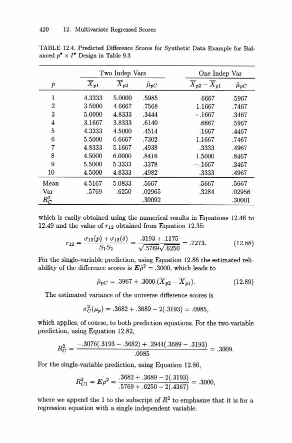
(12.88)

420 12. Multivariate Regressed Scores

TABLE 12.4. Predicted Difference Scores for Synthetic Data Example for Bal­anced p. x r Design in Table 9.3

Two Indep Vars One Indep Var

P X p l X p2 PpC X p2 - X p l PpC

1 4.3333 5.0000 .5985 .6667 .59672 3.5000 4.6667 .7568 1.1667 .74673 5.0000 4.8333 .3444 - .1667 .34674 3.1667 3.8333 .6140 .6667 .59675 4.3333 4.5000 .4514 .1667 .44676 5.5000 6.6667 .7302 1.1667 .74677 4.8333 5.1667 .4938 .3333 .49678 4.5000 6.0000 .8416 1.5000 .84679 5.5000 5.3333 .3378 - .1667 .3467

10 4.5000 4.8333 .4982 .3333 .4967

Mean 4.5167 5.0833 .5667 .5667 .5667Var .5769 .6250 .02965 .3284 .02956R 2 .30092 .30001C

which is easily obtained using the numerical results in Equations 12.46 to12.49 and the value of T1 2 obtained from Equation 12.35:

T12 = 0'12(p) + 0'12(0) = .3193 + .1175 = .7273.8182 V.5769V.6250

For the single-variable prediction , using Equation 12.86 the est imated reli­ability of the difference scores is Eß2 = .3000, which leads to

(12.89)

The estimated variance of the universe difference scores is

O'b(f..Lp) = .3682 + .3689 - 2( .3193) = .0985,

which applies, of course, to both prediction equations. For the two-variableprediction, using Equat ion 12.82,

R2 _ - .3076(.3193 - .3682) + .2944(.3689 - .3193) _C - .0985 - .3009.

For the single-variable prediction, using Equation 12.86,

R2 = E 2 = .3682 + .3689 - 2(.3193) = 3000C l P .5769 + .6250 - 2(.4367) . ,

where we append the 1 to the subscript of R2 to emphasize that i t is for aregression equation with a single independent variable.

12.3 Predicted Composites 421

Table 12.4 provides these two statistics, as well as the observed scoresand predicted values for all persons , for both prediction equations. It isevident from the values of Rb and Rb1 that the two equations are nearlyidentical in terms of their ability to explain the variability in the universedifference scores. This near identity is related to the fact that b1 = -.3076is nearly equal in absolute value to b2 = .2944, both of which are very elosein absolute value to EiP = .3000 for the single-variable regression. Indeed,it can be shown that R2 for the two prediction equations will be equal whenb1 = -b2 , which will occur when PI = P2 and 8 1 = 82 (see Exercise 12.10).

For the two-variable prediction, using Equation 12.75, the standard errorof estimate is

ac(E) = V.0985Vl - .3009 = .2624.

For the single-variable prediction, the standard error of estimate is

aC1 (E) = V.0985Vl - .3000 = .2626.

The near equality of these two estimates is a direct consequence, of course,of the fact that Rb and Rb1 are nearly identical. For either predictionequation, using Equation 12.76, under normality assumptions a 68% tol­erance interval for universe difference scores is approximately Ppc ± .26.This is an interval that is conditional on observed scores, and, as such, itis meaningful to say that 68% of the true difference scores lie within theinterval.

A cursory view of the two sets of predicted values suggests that they aremore different than might be expected, given that the Rb and Rb1 arenearly identical. In particular, note that persons with the same observeddifference score can have different predicted scores for the two-variable re­gression, although they must have the same predicted score for the single­variable regression. This difference is evident , for example, for the secondand sixth persons who have an observed difference of 1.1667. For the secondperson the two-variable prediction is larger than the one-variable predic­tion, but this inequality is reversed for the sixth person . Among otherthings, this means that the tolerance intervals (Equation 12.76) for the twopredictions will be different for persons with the same observed differencescore. By most statistical perspectives (except, perhaps, parsimony) thereis much to recommend the two-variable prediction over its one-variablecounterpart, even when their R2 values are similar.

12.3.3 Different Sample Sizes aiui/or Designs

Prediction equations also can be developed for different sample sizes and/ordesigns. If the design is the same but sample sizes differ, then ar(<5), a~(<5) ,

and a12(<5) will all be affected, as will any statistics based on them, that is,81,82 , pr,P~ , 8 12 , and r12· Otherwise, however, the same equations apply.Prediction equations for the J.: p. design can be estimated by replacing

422 12. Multivariate Regressed Scores

o-type variances and covariances with ß -type variances and covarianceswhich, of course, will affect SI, S2, p~, p~, S12, and T12. For any choice ofsample sizes or design, however, the estimated universe score variances andcovariances still apply, as do the means for the levels of v.

When sample sizes are the same, prediction equations for the p. x JOdesign can be estimated using the same equations and stati stics used for thep. x r design, with one important except ion; namely, TI 2 in Equation 12.88must be replaced by

(12.90)

which is an estimate of the observed correlation when there are no o-typecorrelated errors. This leads to the two-variable prediction

PpC = .5075 - .1794 X pl + .1711 X p2,

with Rb = .1752. Using Equation 12.85, the one-variable predict ion is

PpC = .4676+ .1749 (X p2 - Xpl),

with Rbl = E p2 = .1749.Whether the two-variable or one-variable prediction equation is used, R2

for the p. x J O design is about .17, and R2 for the p. x I" design is about.30. For this synthetic data example, then, the percent of the variance inuniverse difference scores explained by the regression nearly doubles usingthe design that explicitly recognizes correlated errors. This occurs because,for the p. x r design , positively correlated o-type error decreases the stan­dard error of estimate. It follows that , if inter est focuses on using regressionto explain the variance in universe difference scores, then the p. x I" de­sign is preferable to the p. x 1° design if errors are positively correlated. Ofcourse, this conclusion assurnes that the universe of genera lization is onefor which 1 can be "scored" with respect to each level of v. If not , then thep. x I" design is not sensible. When the two scores are pre- and posttestmeasures, this conclusion is consistent with the convent ional wisdom thatsays, "All other things being equal, if you want to measure change, don 'tchange the measure. "

12.3.4 Relationships with Est imated Profiles

For a universe difference score composite, the previous section demon­st rated that , if errors are positively correlated, the p. x I" design yieldsa larger R2 value and a smaller standard error of estimate than the p. x J O

design. By contrast, it was demonstrated in Section 12.2.5 that for regressedscore estimates of individ ual universe scores (Le., predicted profiles) t he

12.3 Predicted Composites 423

p. x r design yields sm aller R 2 values and larger stand ard error of est i­mates than the p. x JO design. In this sense, the "best" design for measur­ing stat us may not the same as the "best" design for measuring differencesor change. This is an example of what might be called an opt imal-design­st ructure paradox, meaning that the "best" design structure for makingdecisions based on regressed score estimates for individual variables maynot be the "best" design st ruct ure for making decisions based on regressedscore est imates for a composite . This is not a statement th at generalizes toall composites , but it definitely can happen.

Let us reexamine the synthetic data results for the two-variable profileand the predicted difference score composite based on two variables:

{lpl 1.4050 + .5339 X p l + .1377 X p2

{lp2 1.8647 + .2263 X p l + .4321 X p2

{lpc .4597 - .3076 X p l + .2944 X p2'

It is immediately evident that {lpc = {lp2 - {lp2. This is a specific exampleof a more general result :

n v

{lpc = L wv{lpv ,v= l

(12.91)

provided t he independent variables for {lpc and the {lpv are the observedscore variables corresponding to the nv universe scores (and only thesevariables). One consequence of Equation 12.91 is that regression coefficientsfor {lpc are easily dete rmined using the regression coefficients for the nvpredictions of /Lpv' Specifically,

n v

bk = L WvbkV'v= l

(12.92)

for k = 0, .. . ,nv . Note that b with one subscript refers to regression coeffi­cients in {lpc , and b with two subscripts refers to regression coefficients in{lpv'

The standard error of estimate for a composite can be determined fromthe variances and covariances of the errors of estimate for the individualvariables:

!7c(E) = V!72 (Lv wv Ev)r--------------

VLv w~ !7~ (E) + L v L v' WvWv' !7vv,(E) , (12.93)

where v =f:. v' for the double summation. For the synthetic data , using thestandard errors of est imate for the two variables computed in Section 12.2.2and the covariance of the errors of estimate computed in Sect ion 12.2.4,

!7c(E) = J( .3572)2 + (.3705)2 - 2(.0980) = .2624,

424 12. Multivariate Regressed Scores

as was obt ained through "direct" computation in Section 12.3.2.R2 for the composite also can be determined using st at ist ics for profile

equations. Two such expressions are:

R~ = (12.94)

(12.95)

where v f; v' in the double summations. For the synt hetic dat a (five-digitversions of the results in Equat ions 12.53, 12.54, and 12.56), Equation 12.94gives

R2 = .24053 + .23164 - 2(.22127) = .3009e .0985 '

and , equivalently, Equation 12.95 gives

R2 = 1 _ (.2624)2 = .3009e .0985 '

as was obtained through "direct" computat ion in Section 12.3.2 .

12.3.5 Other Issues

As discussed in the introduction to Section 12.3, Rb in Equation 12.73 isinterpretable as the proportion of universe composite scores predicted bythe regression or, equivalently, th e squared correlation between universecomposite scores and predicted composite scores. As such, it is a type ofreliability or generalizability coefficient for predicted composites.

Another type of generalizability coefficient for predicted composites is

( A Al )oc J.Lp,J.Lp =

=

L v L vI bvbv'avv'

L v L vI bvbv's.;1 _ L v L vI bvbv,avv,( J)

L v L vI bvbv' s.;1 _ L v L vI bvbv,avv,(J)

L j bj (Lv wvavj) ,

(12.96)

(12.97)

(12.98)

where all subscripts range from 1 to nv . pc(fl,p, fl,~) is interpret able as anestim ate of the correlat ion between predicted composites for two randomlyparallel instances of the measurement procedure. That is, let ting Y andY' be predicted composites for the two parallel procedures, pc( fl,p,fl,~) isthe ratio of their covariance to their variance. Equation 12.97 is a formulafrom classical test theory. Equation 12.98 expresses pc(fl,p,fl,~) in termsof variance and covariance components from a multivariate analysis. The

12.3 Predicted Composites 425

derivation of Equations 12.96 to 12.98 is provided in the answer to Exer­eise 12.13.

The coefficient pc(flp, fl~) is more closely aligned with tradition in mea­surement theory (see, e.g., Feldt & Brennan, 1989, p. 119) than is Rb,but both pc(flp, fl~) and Rb are based on widely accepted, although dif­ferent, definitions of reliability. When nv = 1, the different definitions giveequivalent results.

For purposes of simplicity, and to illustrate conceptual and statisticalissues, most of our treatment of predicted composites has focused on thesimplest case: difference scores and nv = 2 variables. The theory per se,however, has no such restrietion. The general equations provided at thebeginning of Section 12.3 apply to any number of variables and any universescore composite. The principal complexity is that the normal equations(Equations 12.16) with the right-side elements given by Equation 12.70must be solved for the b weights. The b weights are speeific to the D studydesign and sample sizes. Changes in design or sample sizes generally alterthe observed score variances and covariances on the left side of the normalequations, which leads to changes in the b weights.

The theory of predicted composites has been developed here using rawscore regression weights, b. Occasionally, however, predicted compositesbased on ß weights are appropriate. Suppose, for example , that each uni­verse score and raw score is transformed to a T score (not to be confusedwith a true score T) according to the usual formula: T = 50 + 10 Z. Theappropriate regression weights are the ßweights in the prediction equation:

Tpc = ß1Tx 1+ ... + ßkTXk '

where k = n v . These ß weights can be obtained directly through solving thenormal equations in Equation Set 12.15 or, ifthe b weights are available, theß weights are easily determined using Equation 12.17. Since the T scoresare a linear transformation of the Z scores, Rb remains unchanged. UsingEquation 12.75, the standard error of estimate is

Jarjoura (1983) describes a method for obtaining so-called "best" linearpredictions (BLPs) for composite universe scores for the p. x JO design.Jarjoura's BLP equation has a form similar to the predicted-compositeequation for the p. x JO design discussed in this chapter, although thetheory underlying the BLP equation is considerably different. The BLPequation has additional terms related to the category means, which givesit the appearance of a ß-like version of the predicted-composite equationfor the p. x JO design. However, the measurement error variance for theBLP equation is less than O'b(ß). Searle et al. (1992, Chap. 7, especially

426 12. Multivariate Regressed Scores

Sect. 7.4) provide an extensive overview of the statistical theory for BLPs.Applying this theory to the various types of multivariate designs typicallyused in generalizability theory is possible, but not easy.

12.4 Comments

The multivariate perspective on profiles and regressed score estimates dis­cussed in this chapter is very powerful and flexible. The illustrations dis­cussed here have focused on single-facet multivariate designs with n v = 2for simplicity of presentation, but the theory extends readily to any multi­variate design with any number of variables. For raw scores, the essentialsof the process are:

• specify the normal equations in Equation Set 12.16 based on themultivariate design under consideration, using Equation 12.41 forthe rightside of the normal equations when profiles are under con­sideration, or using Equation 12.70 for the right side when predictedcomposites are desired;

• solve the normal equations for the be; and

• use the formulas in Table 12.2 and/or Section 12.2.4 if profiles areunder consideration, or use Equations 12.71 to 12.76 for predictedcomposites.

A similar set of steps applies to standard scores.Many of the most important results in this chapter have been expressed

solely in terms of universe score variance and covariance components, re­gression (b or ß) weights, and apriori (w) weights (when composites areunder consideration) . See, especially, the formulas in Table 12.2 for profilesand Equations 12.70 to 12.75 for predicted composites. This is purposeful.Once universe score variance and covariance components are estimated, re­gression weights are obtained, and apriori weights are specified, just abouteverything else of interest for multivariate regressed scores can be obtained.

The entire discussion of multivariate regressed scores in this chapter hasavoided any consideration of the complexities that arise with unbalanceddesigns in generalizability theory. However, in order to use the theory dis­cussed in this chapter, the variance and covariance components on theright side of the normal equations must be estimated. So, the complex­ities brought about by unbalanced designs are as much an issue here aselsewhere.

Regressed score estimates in multivariate theory have the same potentialfor misuse or misunderstanding that was mentioned in Section 5.5.2 indiscussing regressed score estimates in univariate theory. In particular, thetheory per se does not tell an investigator whether it is sensible to regress

12.5 Exercises 427

scores to the mean of any particular population. In some cases, therefore,applying the theory could have unintended and/or unwanted consequences .It is especially important to be sensitive to such matters when persons'scores are regressed to the mean for their race, gender , or ethnicity. Doingso is not wrong from a statistical perspective, per se, but the investigatorhas the responsibility to provide a substantive, theory-based rationale forchoosing the population(s) used as the referent(s) for scores.

Since the theory discussed in this chapter is essentially an applicationof multiple linear regression analyses, it is natural to think that any com­puter package that performs such analyses can be used in multivariategeneralizability theory. That is not correct, however, because general pur­pose packages require observed values for the dependent variable. For thetheory discussed here, the dependent variable is universe scores for each ofthe separate variables (in the case of regressed score estimates of profiles)or a function of universe scores (in the case of predicted composites) and,of course, universe scores are unknown. For the D study versions of theillustrative designs in Table 9.2, mGENOVA can be used to perform mostof the analyses discussed in this chapter, or at least obtain output thatfacilitates hand computation of desired results. Also, if estimated varianceand covariance components are available, the matrix procedures in SASIML can be used relatively easily to obtain the results in this chapter.

12.5 Exercises

12.1* If Y is the universe score for variable v (i.e., Y = Tv ) , and theindependent variables are the observed scores for all nv variables,show that the relationship between the band ß weights discussedin Section 12.1 is

for j = 1, . . . , nv .

12.2 Equation 12.23 states that rT1X2 = P12(p)VEp~. In classical testtheory, one disattenuation formula is rT1 X2 = rXlx2/VEPt. Whatis the principal source of the difference in these two results?

12.3* Using Equation 12.18, derive Equation 12.52 for a~(flp) ·

12.4 Derive Equation 12.55 for avv,(flp) .

12.5* For nv = 2, prove that R~ ;::: p~ .

12.6 For the synthetic data, Section 12.2.3 derived the result R 12 = .693for raw scores. Verify that this result is the same for standard scores.

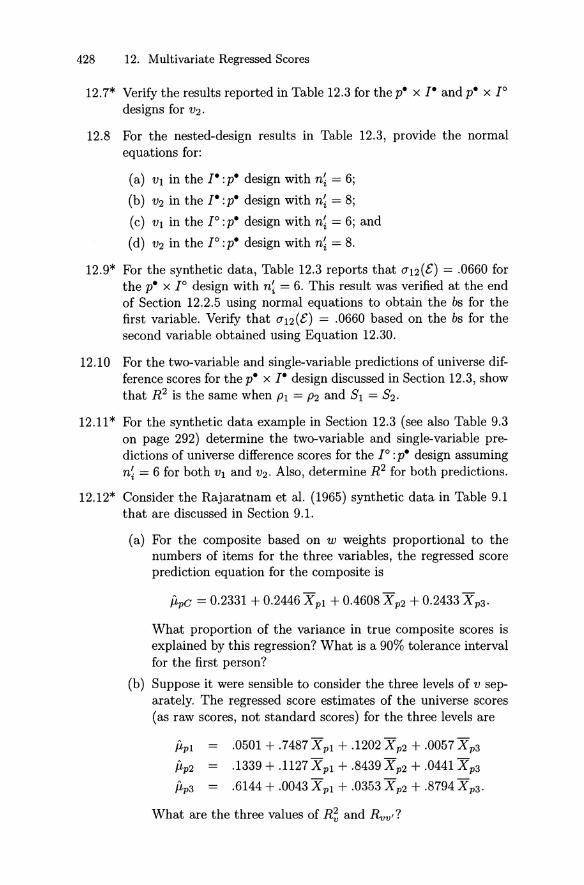
428 12. Multivariate Regressed Scores

12.7* Verify the results reported in Table 12.3 for the p. x J. and p. x JOdesigns for V2 .

12.8 For the nested-design results in Table 12.3, provide the normalequations for:

(a) VI in the I" :p. design with n~ = 6;

(b) V2 in the r :p. design with n~ = 8;

(c) VI in the JO: p. design with n~ = 6; and

(d) V2 in the JO :p. design with n~ = 8.

12.9* For the synthetic data, Table 12.3 reports that 0"12(E) = .0660 forthe p. x JO design with n~ = 6. This result was verified at the endof Section 12.2.5 using normal equations to obtain the bs for thefirst variable. Verify that 0"12(t') = .0660 based on the bs for thesecond variable obtained using Equation 12.30.

12.10 For the two-variable and single-variable predictions of universe dif­ference scores for the p. x r design discussed in Section 12.3, showthat R2 is the same when PI = P2 and SI = S2.

12.11* For the synthetic data example in Section 12.3 (see also Table 9.3on page 292) determine the two-variable and single-variable pre­dictions of universe difference scores for the JO :p. design assumingn~ = 6 for both VI and V2. Also, determine R2 for both predictions.

12.12* Consider the Rajaratnam et al. (1965) synthetic data in Table 9.1that are discussed in Section 9.1.

(a) For the composite based on w weights proportional to thenumbers of items for the three variables , the regressed scoreprediction equation for the composite is

[lpc = 0.2331 + 0.2446 X pI + 0.4608 X p2 + 0.2433 X p3'

What proportion of the variance in true composite scores isexplained by this regression? What is a 90% tolerance intervalfor the first person?

(b) Suppose it were sensible to consider the three levels of v sep­arately. The regressed score estimates of the universe scores(as raw scores, not standard scores) for the three levels are

[lpl .0501+ .7487 X p1 + .1202 X p2 + .0057 X p3

[lp2 .1339 + .1127 Xp 1 + .8439 X p2 + .0441 X p3

[lp3 = .6144 + .0043 X p1 + .0353 X p2 + .8794 X p3 .

What are the three values of R~ and Rvv' ?

12.5 Exercises 429

(c) Suppose the raw scores for the three levels were convertedto so-called T scores (not to be confused with true scores T)according to the usual formula : T pv = 50 + 10 Zpv . What isuvt

12.13 Derive the results in Equations 12.96 to 12.98 for pc(flp, fl~) fora predicted composite with two randomly parallel instances of themeasurement procedure.

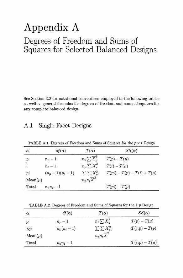
Appendix ADegrees of Freedom and Sums ofSquares for Selected Balanced Designs

See Section 3.2 for notational conventions employed in the following tablesas weIl as general formulas for degrees of freedom and sums of squares forany complet e balanced design.

A.l Single- Facet Designs

TABLE A.1. Degrees üf Freedüm and Sums üf Squares für the p x i Design

a df(a)

pi (np - l)(ni - 1)

Mean(JL)

Tot al npni - 1

T(a) SS(a)

T(p) - T(JL)

T( i) - T(JL)

T(pi) - T(p) - T(i) +T(JL)

T(pi) - T(JL)

TABLE A.2. Degrees of Freedom and Sums of Squares für the i :p Design

a df(a) T(a) SS(a)-2

T(p) - T(JL)p np -1 niLXp

i :p np(ni - 1) LLX;i T(i:p) - T(p)

Mean(JL)-2

npniX

Total npni - 1 T( i :p) - T(JL)

432 Appendix A. Sums of Squares

A.2 Selected Two-Facet Designs

For each of these designs T(J.L) = L: L: L: X;ih' and the total number ofdegrees of freedom is npninh - 1.

TABLE A.3. Degrees of Freedom and Sums of Squares for the p x i x h Design

a df(a) T(a) SS(a)-2

T(p) - T(J.L)p np -1 ninh L:Xp-2

T(i) - T(J.L)ni -1 npnhL:Xi-2

T(h) - T(J.L)h nh -1 npni L:Xh

(np - l)(ni - 1)-2

T(pi) - T(p) - T(i) + T(J.L)pi nh L: L:Xpi

(np - l)(nh - 1)-2

T(ph) - T(p) - T(h) + T(J.L)ph ni L: L:Xph

(ni - l)(nh -1)-2

T(ih) - T(i) - T(h) + T(J.L)ih npL:L:Xih

pih (np - l)(ni - 1) L:L:L:X;ih T(pih) - T(pi) - T(ph) - T(ih)

x (nh -1) +T(p) + T(i) + T(h) - T(J.L)

TABLE AA . Degrees of Freedom and Sums of Squares for the p x (i :h) Design

a df(a)

p np - 1

h nh-1

i :h nh(ni - 1)

ph (np - l)(nh - 1)

pi:h nh(np -l)(ni -1)

T(a) SS(a)

T(p) - T(J.L)

T(h) - T(J.L)

T(i :h) - T(h)

T(ph) - T(p) - T(h) + T(J.L)

T(pi :h) - T(ph)

- T(i :h) + T(h)

A.2 Selected Two-Facet Designs 433

TABLE A.5. Degrees of Freedom and Sums of Squares for the (i :p) x h Design

a df(a)

p n p - 1

h nh-1

i:p np(ni - 1)

ph (np - l)(nh - 1)

ih :p np(ni - l)(nh - 1)

T(a) SS(a)

T(p) - T(/l.)

T(h) - T(Jl)

T(i :p) - T(p)

T(ph) - T(p) - T(h) +T(Jl)

T(ih:p) - T(ph)

- T(i :p) +T(p)

TABLE A.6. Degrees of Freedom and Sums of Squares for the i: (p x h) Design

o df(a)

p n p - 1

h nh- 1

ph (np - l)(nh - 1)

i:ph npnh(ni - 1)

T(a) SS(a)

T(p) - T(Jl)

T(h) - T(Jl)

T(ph) - T(p) - T( h) +T (Jl)

T(i:ph) - T (ph)

TABLE A.7. Degrees of Freedom and Sums of Squares for the (i x h):p Design

a df(a) T(a) SS(a)- 2

T(p) - T(Jl)p n p -1 ninh EXp

np(ni - 1)- 2

T(i :p) - T(p)i:p nhEEXi:p

np(nh - 1)- 2

T(h:p) - T(h)h:p ni E EXh:p

ih :p np(ni - l )(nh - 1) E E EX;ih T(ih:p) - T (i :p)

- T (h:p) +T(p)

TABLE A.8. Degrees of Freedom and Sums of Squares for the i: h :p Design

o

p

h:p

i :h:p

df(a)

np - 1

np(nh - 1)

npnh(ni - 1)

T(a) SS(a)

T(p) - T(Jl)

T(h :p) - T(h)

T(i :h:p) - T( h:p)

Appendix BExpected Mean Squares andEstimators of Random EffectsVariance Components for SelectedBalanced Designs

See Section 3.4 for notational conventions employed in the foIlowing tablesas weIl as general formulas for expected mean squares and estimators ofvariance components for any complete balanced design.

B.I Single-Facet Designs

TABLE B.l. Expected Mean Squares and a-2 (a ) für the p x i Design

0: EMS(o:) &2(0:)

P (J2(pi) + ni(J2(p) [MS(p) - MS(pi)]jni

(J2(pi) + n p(J2(i) [MS(i) - MS(pi)Jln p

pi (J 2(pi) MS(pi)

TABLE B.2. Expected Mean Squares and a-2 (a ) für the i :p Design

EMS(o:)

p

i :p

(J2( i:p) +ni(J2(p)

(J2(i :p)

[MS(p) - MS(i :p)]jni

MS(i :p)

436 Appendix B. Expected Mean Squares

B.2 Selected Two-Facet Designs

TABLE B.3. Expected Mean Squares and o-2(a) für the p x i x h Design

a EMS(a)

p (J'2(pih) + ni(J'2(ph) + nh(J'2(pi) + ninh(J'2(p)

i (J'2(pih) + np(J'2(ih) + nh(J'2(pi) + npnh(J'2(i)

h (J'2(pih) + np(J'2(ih) + ni(J'2(ph) + npni(J'2(h)

pi (J'2(pih) + nh(J'2(pi)

ph (J'2(pih) + ni(J'2(ph)

ih (J'2(pih) + np(J'2(ih)

pih (J'2(pih)

a a-2(a )

p [MS(p) - MS(pi) - MS(ph) + MS(pih)]jninh

i [MS(i) - MS(pi) - MS(ih) + MS(pih)]jnpnh

h [MS(h) - MS(ph) - MS(ih) + MS(pih)]jnpni

pi [MS(pi) - MS(pih)]jnh

ph [MS(ph) - MS(pih)]jni

ih [MS(ih) - MS(pih)]jnp

pih MS(pih)

TABLE BA. Expected Mean Squares and o-2(a) für the p x (i :h) Design

a EMS(a)

p (J'2(pi:h) +ni(J'2(ph) +ninh(J'2(p)

h (J'2(pi:h) + ni(J'2(ph)

+ np(J'2( i:h) + npni(J'2(h)

i:h (J'2(pi :h) + np(J'2(i :h)

ph (J'2(pi:h) + ni(J'2(ph)

pi:h (J'2(pi:h)

[MS(p) - MS(ph)]jninh

[MS(h) - MS(i :h)

- MS(ph) + MS(pi :h)]jnpni

[MS(i:h) - MS(pi :h)]jnp

[MS(ph) - MS(pi :h)]jni

MS(pi :h)

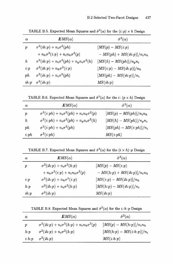
B.2 Selected Two-Facet Designs 437

TABLE B.5. Expected Mean Squares and a-2(a) for the (i :p) x h Design

a EMS(a)

p (J2(ih :p) + ni(J2(ph)

+ nh(J2(i:p) + ninh(J2(p)

h (J2(ih :p) + ni(J2(ph) + npni(J2(h)

i:p (J2(ih:p) + nh(J2(i :p)

ph (J2(ih :p) + ni(J2(ph)

ih:p (J2(ih :p)

[MS(p) - MS(i :p)

- MS(ph) + MS(ih:p)]jninh

[MS(h) - MS(ph)l/npni

[MS(i:p) - MS(ih :p)]jnh

[MS(ph) - MS(ih :p)]jni

MS( ih:p)

TABLE B.6. Expected Mean Squares and a-2 (a ) far the i : (p x h) Design

o EMS(a)

p (J2(i :ph) + ni(J2(ph) + ninh(J2(p)

h (J2(i:ph) +ni(J2(ph) +npnw2(h)

ph (J2(i :ph) + ni(J2(ph)

i:ph (J2(i :ph)

[MS(p) - MS(ph)]jninh

[MS(h) - MS(ph)]jnpni

[MS(ph) - MS(i :ph)]jni

MS(i:ph)

TABLE B.7. Expected Mean Squares and a-2 (a) for the (i x h) :p Design

EMS(a)

p

i:p

h:p

ih:p

(J2(ih:p) + ni(J2(h:p)

+ nh(J2(i:p) + ninh(J2(p)

(J2(ih :p) + nh(J2(i:p)

(J2(ih :p) + ni(J2(h:p)

(J2( ih:p)

[MS(p) - MS(i:p)

- MS(h:p) + MS(ih:p)]jninh

[MS(i:p) - MS(ih :p)]jnh

[MS(h:p) - MS(ih :p)]jni

MS(ih:p)

TABLE B.8. Expected Mean Squares and a-2 (a ) for the i :h:p Design

a EMS(a)

p (J2(ih:p) + ni(J2(h:p) + ninh(J2(p)

h:p (J2(ih :p) + ni(J2(h:p)

i:h:p (J2(ih :p)

[MS(p) - MS(h :p)]jninh

[MS(h:p) - MS(i:h :p)]jni

MS(i:h:p)

Appendix CMatrix Procedures for EstimatingVariance Components and TheirVariability

Parts of the following discussion are based on Searle (1971, pp . 406, 415­417) and Searle et al. (1992, pp . 128-129, 137-138).

C.I Estimated Variance Components

Let j = 1,2, . . . ,k designate the effects in a design (main effects and inter­action effects, hut not J.L) . Also, let

{

k X k upper-triangular matrix of coefficients of the vari­P = ance components in the EMS equations for the model

(random, mixed, or sampling from a finite universe),

and

a = k x 1 column vector of mean squares for the design .

Then,(C.l)

is a k x 1 column vector whose elements are unbiased estimates of thevariance components. For a random model, these estimates are identical tothose resulting from using the algorithm in Section 3.4.4. For any model,the estimates in Equation C.l are the same as those obtained using thealgorithm in Section 3.4.4 in conjunction with Equation 3.34. For a mixedmodel, the "varianees" associated with fixed effects are called quadraticforms in traditional statistical literature .

440 Appendix C. Matrix Procedures for Variance Components

C.2 Variability of Estimated Variance Components

Estimated variance components are themselves subject to sampling vari­ability. Furthermore, two estimated variance components are generally notuncorrelated, unless there are no common mean squares used in estimatingthe two variance components.

C.2.1 Single Conditions

Assuming a multivariate normal distribution for the score effects, the sym­metrie variance-covariance matrix associated with the estimated variancecomponents in Equation C.l is

(C.2)

whereD _ {k x kdiagonal matrix containing the (C 3)

1 - diagonal elements 2(M Sj )2 j (dJi + 2), .

and(p-I)' means the transpose of p-I.

The diagonal elements of V are unbiased estimators of the variances ofthe estimated variance components, under the normality assumption. Theirsquare roots have been denoted previously as 0-[0-2(a)J or 0-[0-2(aIM)J .

C.2.2 Mean Scores

The symmetrie matrix V provides the estimated variances and covariancesassociated with the 0-2(aIM), which are estimated variance components forsingle conditions. There is a corresponding variance-covariance matrix asso­ciated with the 0-2(äIM'), that is, with the estimated variance componentsfor means over n' conditions from facets in the universe of generalization(see Equation 5.1). If N' = N for each facet and the G and D study designshave the same structure, then this variance-covariance matrix is

(CA)

where

D = {k x kdiagonal matrix with elements C(älr)jd(älr), where d(älr)2 and C(älr) are defined by Equations 5.2 and 5.3, respectively.

The square roots of the diagonal elements in Ware the estimated stan­dard errors of the variance components associated with mean scores. Theyhave been denoted previously as 0-[0-2(ä)] and 0-[0-2(äIM)] .

(C.5)

C.3 Example 441

Using the symmetrie matrix W, the estimated standard error of 0-2(.6..)

is

{

square root of the sum of the elements in W0-[0-2(~)] = excluding those rows and columns of W as­

sociated with effects that do not enter .6...

As indieated below, the standard errors of 0-2(8) and Est[ES2(p)J can beestimated in a similar manner.

C.3 Example

Table C.I provides the vectors and matrices in Equations C.I and C.2 forthe p x (r :t) design using Synthetic Data Set No. 4 in Table 3.2 on page 73.Row and column j = 1,2,3,4, and 5 correspond to Cl = p, t, r:t pt, andpr:t , respectively. The square roots of the diagonal elements of V are theestimated standard errors of the G study estimated random effects variancecomponents. _

Table C.I also provides the D 2 and W matriees in Equation C.4 assum­ing n~ = 3 and n~ = 4. The square roots of the diagonal elements in Warethe estimated standard errors denoted previously as 0-[0-2(ä)J. For example ,

0-[0-2(pR)] = V.0158 = .126.

Since 0-2(.6..) is the sum of all the 0-2(ä) except 0-2(p), the estimatedstandard error of 0-2(~) is the square root of the sum of all entries in Wexcept those in the first row and column:

0-[0-2(.6..)] = v.0322 = .179.

Since 0-2(8) = 0-2(pR) + 0-2(pI:R), the estimated standard error of 0-2(8) isthe square ~t of the sum of all entries in the fourth and fifth rows andcolumns of W :

0-[0-2(8)] = V.0149 = .122.

Since Est[ES2(p)] includes all the 0-2(ä) except 0-2(T) and 0-2(R:T), theestimated standard error of Est[ES2(p)] is the square root of the sum ofall entries in W except those in the second and third rows and columns :

0-[Est[ES2(p)J] = V.1340 = .366.

CA Complex Cases

Equation CA is appropriate when N' = N for each facet . If this conditionis not fulfilled, then there is a transformation matrix T that converts the

442 Appendix C. Matrix Procedures for Variance Components

TABLE C.I. Matrices for Obtaining Estimated Variance Components and Stan­dard Errors for Synthetic Data Set No. 4

12 0 0 4 140 10 4 1

p= 10 0 14 1

1

.083 .0000 .0000 -.0833 .0000.0250 -.0250 - .0250 .0250

p-l= .1000 .0000 - .1000.0250 -.0250

1.0000

10.2963 .473124.1000 .32528.8556 - 2 .6475a= (J' =4.6185 .55962.3802 2.3802

[ 19.2752290.4050

13J

D 1 = 14.25832.1331

[ .1487.0044 .0000 - .0444 .0000

.0044 .1918 - .0360 - .0142 .0034V = .0000 -.0360 .1439 .0034 - .0137

-.0444 -.0142 .0034 .1418 -.0341.0000 .0034 -.0137 .0341 .1365

1.0000.3333

D2= .0833.3333

.0833

.1487 .0015 .0000 -.0148 .0000

.0015 .0213 - .0010 - .0016 .0001-w= .0000 - .0010 .0010 .0001 - .0001- .0148 -.0016 .0001 .0158 -.0009

.0000 .0001 - .0001 - .0009 .0009

CA Complex Cases 443

o-2(aIM) associated with facets of size N to the o-2(aIM') associated withfacets of size N'. For example, to convert the o-2(a) for Synthetic Data SetNo. 4 to the o-2(aIT) in Table 5.2, the transformation matrix is

1 0 0 .33 01 0 0 0

T= 1 0 01 0

1

and the o-2(aIM') are the elements ofthe vector T&2 . Given T, the variance­covariance matrix associated with the o-2(CiIM') is

(C.6)

When a fixed facet occurs as ~rimary index in Ci, all entries in the corre­sponding row and column of W will be zero.

Also, Equation CA assurnes that the G and D study designs have thesame structure. Consider, however, the possibility that the G study designis p x (r :t), the D study design is R :T :p, and both models are random. Inthis case, the transformation matrix is:

[100 0 0]

T= 1 0 1 0 ,101

where the sequence of the columns is a = p, t , r :t , pt, pr:t, and the se­quence of the.!.ows is a = p, t:p , r:t:p. For this transformation matrix,both D2 and Ware 3 x 3 matrices.

Appendix DTable for Simplified Use ofSatterthwaite's Procedure

Section 6.2.2 describes Satterthwaite's (1941, 1946) pro cedure for placingconfidence intervals on variance components. A simplified version of thatprocedure employs the mult iplicative factors:

1 . li t: 1 1" 2r2

mu ti p ier ror ower imit = 2 ( 2)Xu 2r

and2r 2

multiplier for upper limit = 2( 2)XL 2r

in Equations 6.20 and 6.21, respect ively, where X~ (v) and XI(v) are thelouier U = (1+, )/2 and L = (1 - ,) /2 percentile points of the chi-squareddistribution with v = 2r2 effective degrees of freedom. Table D.1 tabulatesthese multiplicative factors for 66.67, 80, 90, and 95% confidence interva ls.!

IThe values reported here are a subset of t hose provided in Bre nnan (1992a).

446 Appendix D. Satterthwaite's Procedure

TABLE D.l. Multiplicative Factors for lOO(-y)% Confidence Intervals on VarianceComponents

66.67% 80% 90% 95%v r Lower Upper Lower Upper Lower Upper Lower Upper

8 2.000 0.6855 1.8801 0.5987 2.2927 0.5157 2.9282 0.4560 3.67168.5 2.062 0.6915 1.8356 0.6060 2.2217 0.5240 2.8100 0.4647 3.4903

9 2.121 0.6970 1.7960 0.6128 2.1595 0.5318 2.7076 0.4729 3.33509.5 2.179 0.7022 1.7612 0.6193 2.1046 0.5392 2.6181 0.4806 3.200410 2.236 0.7071 1.7299 0.6254 2.0558 0.5461 2.5392 0.4879 3.0827

10.5 2.291 0.7118 1.7018 0.6312 2.0120 0.5527 2.4678 0.4950 2.976311 2.345 0.7162 1.6763 0.6366 1.9726 0.5589 2.4048 0.5016 2.8837

11.5 2.398 0.7203 1.6531 0.6418 1.9368 0.5649 2.3481 0.5079 2.800812 2.449 0.7243 1.6318 0.6469 1.9037 0.5706 2.2967 0.5139 2.7262

12.5 2.500 0.7281 1.6122 0.6516 1.8738 0.5760 2.2499 0.5198 2.658613 2.550 0.7317 1.5942 0.6561 1.8463 0.5812 2.2071 0.5253 2.5971

13.5 2.598 0.7352 1.5775 0.6604 1.8210 0.5862 2.1677 0.5307 2.540914 2.646 0.7385 1.5619 0.6646 1.7975 0.5909 2.1315 0.5358 2.4893

14.5 2.693 0.7417 1.5474 0.6685 1.7756 0.5955 2.0980 0.5408 2.440215 2.739 0.7447 1.5339 0.6723 1.7553 0.6000 2.0661 0.5455 2.3961

15.5 2.784 0.7477 1.5212 0.6760 1.7362 0.6042 2.0371 0.5500 2.355316 2.828 0.7506 1.5093 0.6795 1.7184 0.6083 2.0100 0.5544 2.3173

16.5 2.872 0.7533 1.4979 0.6829 1.7017 0.6123 1.9846 0.5587 2.281817 2.915 0.7559 1.4873 0.6863 1.6860 0.6161 1.9608 0.5629 2.2487

17.5 2.958 0.7585 1.4773 0.6895 1.6711 0.6198 1.9384 0.5669 2.217618 3.000 0.7609 1.4678 0.6925 1.6568 0.6233 1.9173 0.5707 2.1884

18.5 3.041 0.7633 1.4588 0.6955 1.6435 0.6269 1.8974 0.5745 2.159919 3.082 0.7656 1.4503 0.6984 1.6309 0.6302 1.8786 0.5781 2.1339

19.5 3.122 0.7678 1.4421 0.7012 1.6189 0.6335 1.8608 0.5817 2.109420 3.162 0.7699 1.4344 0.7039 1.6075 0.6366 1.8434 0.5851 2.086121 3.240 0.7741 1.4199 0.7090 1.5863 0.6426 1.8120 0.5917 2.043222 3.317 0.7779 1.4067 0.7139 1.5669 0.6483 1.7834 0.5980 2.004423 3.391 0.7816 1.3946 0.7185 1.5492 0.65 38 1.7574 0.603 8 1.968 324 3.464 0.7851 1.3834 0.7229 1.5329 0.6 590 1.7335 0.6094 1.935925 3.536 0.7884 1.3730 0.7271 1.5178 0.6638 1.7115 0.6149 1.906326 3.606 0.7915 1.3633 0.7310 1.5037 0.6685 1.6908 0.6200 1.879027 3.674 0.7945 1.3543 0.7348 1.4907 0.6730 1.6719 0.6249 1.853728 3.742 0.7974 1.3458 0.7384 1.4785 0.6772 1.6544 0.6296 1.829629 3.808 0.8002 1.3379 0.7418 1.4671 0.6813 1.6380 0.6340 1.807830 3.873 0.8028 1.3305 0.7451 1.4565 0.6852 1.6226 0.6384 1.787431 3.937 0.8053 1.3235 0.7483 1.4465 0.6890 1.6082 0.6425 1.768332 4.000 0.8077 1.3169 0.7514 1.4370 0.6926 1.5945 0.6465 1.749933 4.062 0.8100 1.3106 0.7543 1.4281 0.6961 1.5817 0.6504 1.733134 4.123 0.8123 1.3047 0.7571 1.4197 0.6994 1.5696 0.6541 1.717235 4.183 0.8144 1.2991 0.7598 1.4117 0.7027 1.5582 0.6576 1.702236 4.243 0.8165 1.2938 0.7624 1.4039 0.7058 1.5474 0.6611 1.688037 4.301 0.8185 1.2887 0.7650 1.3967 0.7088 1.5372 0.6645 1.674238 4.359 0.8204 1.2839 0.7674 1.3898 0.7117 1.5275 0.6677 1.661439 4.416 0.8222 1.2793 0.7698 1.3833 0.7145 1.5180 0.6709 1.649340 4.472 0.8242 1.2745 0.7723 1.3767 0.7174 1.5090 0.6740 1.637841 4.528 0.8260 1.2703 0.7745 1.3707 0.7201 1.5005 0.6770 1.626742 4.583 0.8277 1.2662 0.7766 1.3650 0.7227 1.4924 0.6798 1.616143 4.637 0.8293 1.2623 0.7787 1.3595 0.7251 1.4846 0.6826 1.605944 4.690 0.8309 1.2586 0.7807 1.3542 0.7276 1.4772 0.6853 1.596245 4.743 0.8324 1.2550 0.7827 1.3491 0.7299 1.4700 0.6879 1.5869

Appendix D. Satterthwaite's Procedu re 447

TABLE D.2. Multiplicative Factors for lOO(-y)% Confidence Intervals on VarianceComponents (continued)

66 .67% 80% 90 % 95 %v r Lower Upper Lower Upper Lower Upper Lowe r Upper

46 4 .796 0.8339 1.2516 0.7845 1.3442 0 .7322 1.4632 0.6905 1.578047 4.848 0 .8354 1.2483 0 .7864 1.3396 0 .7344 1.4566 0.6930 1.569448 4.899 0 .8368 1.2451 0 .7882 1.3350 0 .7366 1.4503 0.6954 1.561249 4 .950 0 .8382 1.2420 0 .7899 1.3307 0 .7387 1.4442 0.6978 1.553350 5.000 0 .8395 1.2390 0 .7916 1.3265 0 .7407 1.4383 0 .7001 1.545751 5.050 0 .8408 1.2 361 0 .7933 1.3224 0 .7427 1.4326 0 .7023 1.538352 5.099 0.8421 1.2333 0.7949 1.3185 0 .7447 1.4271 0.7045 1.531253 5.148 0.8433 1.2306 0.7965 1.31 47 0 .7466 1.4219 0.7066 1.524454 5.196 0.8445 1.2280 0.7980 1.3 111 0 .7485 1.4 167 0 .708 7 1.517 855 5.244 0 .8457 1.2255 0.7995 1.3075 0 .7503 1.411 8 0 .7 107 1.5 11456 5 .292 0.8469 1.2230 0 .80 10 1.3041 0 .7520 1.4070 0 .7127 1.505257 5.339 0 .8480 1.2207 0 .8025 1.3008 0 .7538 1.4024 0 .7147 1.499358 5.385 0.8491 1.2184 0.80 39 1.2975 0 .7555 1.3979 0. 7166 1.493559 5.431 0.8502 1.2161 0 .80 52 1.2944 0 .7571 1.3935 0.7185 1.487960 5.477 0.85 12 1.2139 0.8066 1.2913 0.7587 1.3893 0.7203 1.482461 5.523 0 .8522 1.2118 0.8079 1.2884 0 .7603 1.3852 0 .7221 1.477262 5.568 0.8532 1.2098 0.8092 1.2855 0 .7619 1.3812 0.7238 1.472063 5.612 0.8542 1.2078 0.8104 1.2827 0 .7634 1.3773 0.7255 1.467164 5.657 0 .8552 1.2058 0.8116 1.2800 0 .7649 1.3736 0.7272 1.462265 5.701 0.8561 1.2039 0.812 8 1.2773 0 .7664 1.3699 0.7289 1.457566 5.745 0.8570 1.2021 0.8140 1.2748 0 .7678 1.3663 0 .7305 1.453067 5.788 0 .8579 1.2003 0.8 152 1.2722 0 .7692 1.3628 0 .7321 1.448568 5.831 0.85 88 1.1985 0.8163 1.2698 0 .7706 1.3595 0.7336 1.444269 5.874 0. 8597 1.19 68 0 .8174 1.2674 0 .7719 1.3562 0 .7351 1.440070 5.916 0 .8606 1.1951 0 .8185 1.2651 0 .7732 1.3529 0 .7366 1.435971 5.958 0 .8614 1.1935 0.8196 1.2628 0 .7745 1.3498 0.73 81 1.431972 6.000 0 .8622 1.1919 0 .8206 1.2606 0 .77 58 1.3468 0 .7396 1.428073 6.042 0.8630 1.1903 0.82 17 1.2584 0.7771 1.34 38 0.7410 1.4 24274 6 .083 0 .8638 1.1888 0 .8227 1.2563 0 .7783 1.3408 0.7424 1.420575 6. 124 0.8 646 1.1873 0 .8237 1.2542 0 .7795 1.3380 0 .7437 1.416876 6.164 0.8654 1.1859 0 .8247 1.2522 0 .7807 1.3352 0 .7451 1.413377 6.205 0 .8661 1.1844 0 .82 56 1.2502 0 .7819 1.3325 0 .7464 1.409878 6 .245 0.86 68 1. 1830 0.826 6 1.2483 0 .7830 1.3298 0.7477 1.406479 6.285 0.8676 1.1817 0 .8275 1.2464 0.7842 1.3272 0.7490 1.403180 6 .325 0.8683 1.180 3 0.8284 1.2445 0 .78 53 1.3247 0.7502 1.399981 6 .364 0.8690 1.1790 0.8293 1.2427 0 .7864 1.3222 0 .7515 1.396782 6.403 0 .8697 1.1777 0.8302 1.2409 0 .7874 1.3198 0.7527 1.393783 6 .442 0.8703 1.1765 0.8310 1.2392 0 .7885 1.3174 0.7539 1.390684 6 .481 0.8710 1.1753 0 .8319 1.2375 0 .7895 1.3150 0.755 1 1.387785 6.5 19 0 .8717 1.1740 0 .832 7 1.2358 0 .7906 1.3128 0.7563 1.384886 6 .55 7 0 .87 23 1.1729 0.8336 1.2342 0 .7916 1.3105 0.7574 1.381987 6.595 0.8729 1. 1717 0 .8344 1.2326 0 .7926 1.3083 0.7585 1.3 79188 6.633 0.8736 1.1706 0.8352 1.2310 0 .7935 1.3062 0.7596 1.376489 6 .671 0.8742 1.1694 0.8360 1.2294 0 .7945 1.3040 0.7607 1.3 73790 6.708 0.8748 1.1683 0.8367 1.2279 0 .7955 1.3020 0.7618 1.371195 6.892 0.8777 1.1631 0.840 5 1.2207 0 .8000 1.2922 0.7670 1.3587

100 7.071 0.8804 1.1584 0.8439 1.2 142 0 .8043 1.2832 0.771 8 1.3474105 7.246 0.8829 1.1540 0 .8472 1.2081 0 .80 82 1.2750 0.7763 1.3371110 7.416 0.8853 1.14 99 0.8502 1.2025 0 .8119 1.2674 0 .7806 1.3275115 7.583 0.8875 1.1 462 0 .8531 1.1973 0 .81 54 1.2604 0.7846 1.3 187

448 Appendix D. Satterthwaite's Procedure

TABLE D.3. Multiplicative Factors for 100(.,,)% Confidence Intervals on VarianceComponents (continued)

66 .67% 80% 90% 95%

v r Lower Upper Lower Upper Lower Upper Lower Upper

120 7.746 0.8896 1.1427 0.8558 1.1925 0.8188 1.2539 0.7884 1.3105130 8.062 0.8934 1.1363 0.8607 1.1838 0 .8248 1.2421 0.7953 1.2958140 8.367 0.8969 1.1307 0.8651 1.1761 0.8303 1.2317 0.8016 1.2828150 8.660 0.9000 1.1258 0.8692 1.1693 0.8353 1.2226 0.8073 1.2714160 8 .944 0.9028 1.121 3 0.8729 1.1632 0.8398 1.2144 0.8125 1.2612170 9 .220 0.9054 1.1173 0.8762 1.1577 0 .8440 1.2070 0.817 3 1.2520180 9.487 0.9078 1.1136 0.879 3 1.1527 0.8478 1.2002 0.8217 1.2436190 9 .747 0.9101 1.1102 0.8822 1.1481 0.8514 1.1941 0.8259 1.2360200 10.000 0.9121 1.1071 0.8849 1.14 39 0.8547 1.1885 0.8297 1.2291210 10.247 0.9140 1.1043 0.8874 1.1400 0 .8578 1.1833 0.8332 1.2227220 10.488 0.9158 1.1017 0.8897 1.1364 0.8607 1.1785 0.8366 1.2167230 10.724 0.9175 1.0992 0.8919 1.1331 0.8634 1.1741 0.8397 1.2113240 10.954 0.9191 1.0969 0.8940 1.1300 0.8660 1.1700 0.8427 1.2061250 11.180 0.9206 1.0948 0.8959 1.1271 0.8684 1.1661 0.8455 1.2014300 12.247 0.9270 1.0858 0 .9042 1.1150 0.8788 1.1500 0.8574 1.1815350 13.229 0 .9320 1.0790 0 .9107 1.1057 0.8869 1.1377 0.8669 1.1664400 14.142 0 .9361 1.0735 0 .9161 1.0983 0.8936 1.1279 0.8747 1.1545450 15.000 0.9395 1.0690 0.9205 1.0922 0 .8992 1.1199 0.8812 1.1447500 15.811 0.9425 1.0652 0.9243 1.0871 0 .9040 1.1132 0.8868 1.1365550 16.583 0.9450 1.0620 0.9276 1.0828 0 .9081 1.1075 0.8916 1.1296600 17.321 0.9472 1.0592 0.930 5 1.0790 0.9117 1.1026 0.8958 1.1236650 18.028 0.9492 1.0567 0.9331 1.0757 0.9150 1.0982 0.8996 1.1183700 18.708 0.9509 1.0546 0.9354 1.0728 0.9178 1.0944 0 .9030 1.1136750 19.365 0.9525 1.0526 0.9375 1.0702 0.920 5 1.0910 0.9060 1.1095800 20.000 0.9539 1.0509 0.9393 1.0678 0.9 228 1.0879 0 .9088 1.1057850 20.616 0 .9552 1.0493 0.9411 1.0657 0.9250 1.0851 0.9113 1.1023900 21.213 0.9564 1.0478 0.9426 1.06 37 0 .9270 1.0825 0.9137 1.0992950 21.794 0.9576 1.0465 0.9441 1.0619 0.9288 1.0802 0.9158 1.0964

1000 22 .361 0.9586 1.0452 0.9454 1.0603 0.9305 1.0781 0.9178 1.09381500 27 .386 0.9659 1.0366 0.9550 1.0488 0.9427 1.0630 0.9321 1.07562000 31.623 0 .9703 1.0316 0.9609 1.0420 0.9501 1.0542 0.9408 1.06502500 35 .355 0 .9734 1.0281 0.9649 1.0374 0.9551 1.0483 I 0.9468 1.05783000 38. 730 0 .9756 1.02 56 0 .9678 1.03 41 0.9589 1.0439 0 .9513 1.05263500 41.833 0.9774 1.02 37 0.9702 1.0315 0.9619 1.0406 0 .9548 1.04864000 44 .721 0.9788 1.0221 0 .9720 1.0294 0.9643 1.0379 0 .9576 1.04534500 47.434 0.9800 1.0208 0 .9736 1.0277 0.9663 1.0356 0 .9599 1.04265000 50 .000 0.9810 1.0197 0.9749 1.0262 0.9679 1.03 38 0 .9619 1.04045500 52.440 0.9819 1.0188 0 .9761 1.0250 0.9694 1.0322 0.9637 1.03856000 54 .772 0.9827 1.0180 0.9771 1.02 39 0.9707 1.0308 0.9652 1.03686500 57 .009 0.9833 1.0173 0.9780 1.0229 0 .9718 1.0295 0.966 5 1.03537000 59.161 0.9839 1.0166 0.9787 1.0221 0.9728 1.0284 0.9677 1.03407500 61.237 0.9845 1.0161 0.9795 1.0213 0.9737 1.0274 0 .9688 1.03288000 63 .246 0.9849 1.0155 0.9801 1.0206 0.974 5 1.0266 0.9697 1.03178500 65 .192 0 .9854 1.0151 0.9807 1.0200 0.975 3 1.0257 0.970 6 1.03089000 67 .082 0 .9858 1.0146 0.9812 1.0194 0.9759 1.0250 0.9714 1.02999500 68 .920 0 .9862 1.0142 0.9817 1.0189 0 .9766 1.0243 0.9722 1.0291

10000 70 .711 0 .9865 1.0139 0.9822 1.0184 0.9772 1.0237 0.9729 1.028315000 86 .603 0 .9890 1.011 3 0.9854 1.0150 0.9813 1.0193 0.9778 1.023020000 100 .000 0 .9904 1.0098 0.9873 1.0130 0.9838 1.0167 0.9807 1.01 99

Appendix EFormulas for Selected UnbalancedRandom Effects Designs

Section 7.1 provides analogous-ANOVA formulas for est imating randomeffects variance components for the i :p and p x (i: h) designs th at are un­balanced with respect to nest ing, as weil as the p x i design that is un­balanced with respect to missing data. Here, formulas are provided for theunbalanced i: h :p and (p: c) x i designs.

U nbalanced i: h : p Design

For the unbalanced i : h :p design nh:p is the number of levels of h for eachp, and ni:h :p is the number of levels of i for each level of h and p. We alsodefine

n ., = total number of observat ions in design,

n h+ = L:p nh:p = total number of levels of h,

np = the number of observat ions for a particular p, and

Given these notat ional convent ions, the degrees of freedom, T te rrns, andsums of squares are given in the following table.

450 Appendix E. Selected Unbalanced Designs

Effect df T SS-2

T(p) - T(/1)p np - 1 2:p npXp- 2

T(h :p) - T(p)h:p nh+ - np 2:p 2:h nphX ph

i :h:p n+ - nh+ 2:p 2:h 2:iX;ih T( i :h:p) - T(h:p)

Meantu)-2

1 n+X

Letting-2 - 2 -2

Tpi = 2:2: i h, Ti = 2:2: n

ph, and ro. = 2: n

p,

p h P P h n+ p n.,

the coefficient s of /12 and the variance components in t he expected T termsare given in t he following table.

Coefficient s

E T /12 (J'2(i :h:p) (J'2(h:p) (J'2(p)

E T (p) n+ np Tpi n+

ET(h:p) n+ nh+ n + n+

E T (i:h:p) n+ n+ n+ n+

E T (/1) n+ 1 Ti Tih

It follows that the expected mean square equations are

E MS (p) =

E MS (h:p) =

E MS (i:h:p)

E T (p) - E T (/1 )np -1

= (J'2(i:h:p) + (TPi - Ti ) (J'2(h:p) + (n+ - Tih) (J'2(p)np- l n p -l

E T (h:p) - E T (p)

nh+ - np

(J'2(i:h :p) + ( n+ - Tpi ) (J'2(h:p)nh+ - np

ET(i :h:p) - E T (h:p)

n+ - nh+

= (J'2(i :h:p).

It is possible to use these expected mean square equat ions to obtainestimators of the variance components, but it is easier to use the expectedT t erms . The results are :

a-2(i:h:p) = T( i:h:p) - T(h:p)

Appendix E. Selected Unbalanced Designs 451

n+ - rpi

T(p) - T(J-l) - (np - 1)a2(i :h:p) - (rpi - r i )a2(h:p)

Using different notational conventions, these results are reported by Searleet al. (1992, p. 429).

U nbalanced (p: c) X i Design

For the unbalanced (p :c) x i design, let np :e be the number of levels of pfor each c. We also define

n+ = total number of observat ions in design and

np+ = L:enp :e = total number of levels of p.

Given these notational conventions, the degrees of freedom and T termsare given in the following table.

Effect

c

p:c

ci

pi :c

Meanfe)

Letting

df

ni - 1

(n e - l)(n i - 1)

(n p+ - ne)(n i - 1)

1

T

and

the coefficients of J-l2 and the variance components in the expected T termsare given in the following table.

Coefficients

ET J-l2 O'2(pi :c) 0'2 (ci) 0'2 (i) O'2(p: c) O'2(c)

ET(c) n+ ne np+ np+ neni n+

ET(p:c) n+ np+ np+ np+ n+ n+

ET(i) n+ ni nir p n+ ni nirp

ET(ci) n+ neni n+ n+ neni n+

ET(pi:c) n+ n+ n+ n+ n+ n+

ET(J-l) n+ 1 r p np+ ni nirp

452 Appendix E. Selected Unbalanced Designs

Using matrix procedures the T-term equations can be solved for estimatesof the variance components.

Alternatively, the expected mean square equations can be determined,and they can be used to obtain estimates. The expected mean square equa­tions are:

EMS(c) = a2(pi:c) + tpa2(ci)+ ni a2(p:c)+ tpni a2(c)

EMS(p:c) = a2(pi:c) + ni a2(p:c)

EMS(i) = a2(pi:c)+rpa2(ci)+np+a2(i)

EMS(ci) = a2(pi:c)+ tpa2(ci)

EMS(pi :c) = a2(pi:c).

Estimators of the variance components in terms of mean squares are:

8'2(C) = [MS(c) - MS(p:c) - MS(ci) + MS(pi:c)]/nitp

8'2(p:C) = [MS(p:c) - MS(pi:c)]/ni

8'2(i) = [MS(i) - rpMS(ci)jtp+ (rp - tp)MS(pi :c)jtp]/np+8'2(ci) = [MS(ci) - MS(pi :c)]/tp

8'2(pi:c) = MS(pi:c).

Appendix FMini-Manual for GENOVA

GENOVA (GENeralized analysis Of VAriance) is a FORTRAN computerprogram developed principally for generalizability analyses, although itis also useful for more traditional applications of analysis of variance.GENOVA is appropriate for complete balanced designs with as many assix effects (l.e., five facets and an objects of measurement "facet") .

Crick and Brennan (1983) provide an extensive manual for GENOVA.This appendix is a mini-manual that illustrates those features and capabil­ities of GENOVA that are most likely to be used in typical generalizabilityanalyses . GENOVA and program documentation can be obtained from theauthor (robert-brennan@uiowa.edu) or from the Iowa Testing ProgramsWeb site (www.uiowa.eduritp). At this time , both PC and Macintoshversions of GENOVA are available free of charge.

F.1 Sample Run

Provided in Table F.1 are the control cards and input data for a run ofGENOVA in which the G study is based on Synthetic Data Set No. 4 (seeTable 3.2 on page 73) for the p x (r: t) random effects design having 10persons (p), three tasks (t), and four raters (r) nested within each of thethree tasks. The control cards for the G study are numbered 1 to 7, and thedata cards (records) are numbered 8 to 17. These card numbers are usedhere for reference purposes only; they are not part of the control cardsthemselves.

454 Appendix F . GENOVA

TABLE F.l. Control Cards for Genova Using Synthetic Data Set No. 4

CARD COLUMNS 111111111122222222223333333333444444444455555555NO. 123456789012345678901234567890123456789012345678901234567

SECOND SET OF D STIJOY CONTROL CARDS#2 -- R:T :P DESIGN -- RAND TRANDOM$ P

T:P 3R:T:P 1 2 3 4

FIRST SET OF D STIJOY CONTROL CARDS#1 -- P X (R:T) DESIGN -- RAND TRANDOM$ P

T 3R:T 1 2 3 4

THIRD SET OF D STIJOY CONTROL CARDS#3 -- P X CR :T) DESIGN -- R RANDDM,$ P

T 3 / 3R:T 1 2 3 4

P X (R:T) DESIGN -- RANDOM MODELRECORDS 2* P 10 0+ T 3 0+ R:T 4 0(12F2.0)

T FIXED

PERSON 1PERSON 2PERSON 3PERSON 4PERSON 5PERSON 6PERSON 7PERSON 8PERSON 9PERSON 10

1 GSTIJOY2 OPTIONS3 EFFECT4 EFFECT5 EFFECT6 FORMAT7 PROCESS8 5 6 5 5 5 3 4 5 6 7 3 399377 7 5 557 7 5 2

10 3 4 3 3 5 3 3 5 6 5 1 611 7 5 5 3 3 1 4 3 5 3 3 512 9 2 9 7 7 7 3 7 2 7 5 313 3 4 3 5 3 3 6 3 4 5 1 214 7 3 7 7 7 5 5 7 5 5 5 415 5 8 5 7 7 5 5 4 3 2 1 116 9 9 8 8 6 6 6 5 5 8 1 117 4 4 4 3 3 5 6 5 5 7 1 118 COMMENT19 COMMENT20 DSTIJOY21 DEFFECT22 DEFFECT23 DEFFECT24 ENDDSTIJOY25 COMMENT26 DSTIJOY27 DEFFECT28 DEFFECT29 DEFFECT30 ENDDSTIJOY31 COMMENT32 DSTIJOY33 DEFFECT34 DEFFECT35 DEFFECT36 ENDDSTIJOY37 FINISH

F.2 G Study Control Cards 455

GENOVA can use G study estimated variance components to estimateresults for various D study designs. For the sample run of GENOVA, thereare three sets of D study control cards. The first set (card numbers 20 to24) is for random effects D studies for the p x (R :T) design. The secondset (card numbers 26 to 30) is for random effects D studies for the R: T :pdesign. The third set (card numbers 32 to 36) is for the p x (R :T) designwith tasks fixed and raters random.

Each control card begins with a set of characters called a control cardidentifier in columns 1 to 12. (Actually, GENOVA pays attention only tothe first four characters.) All parameters in GENOVA control cards mustappear in columns 13 to 80 and are in free format. Neither control cardidentifiers nor parameters should use lowercase letters. If there are multipleparameters, they must be provided in the specified order, but they do notneed to be placed in specific columns. It is only necessary that multipleparameters be separated by at least one comma and/or one space.

COMMENT cards may appear anywhere except within, or immediately be­fore, an input data set . Any alphanumeric text may appear in columns 13to 80 of a COMMENT card .

F.2 G Study Control Cards

The GSTUDY control card provides nothing more than a heading, KTITLE,for the run. For this example , the heading verbally specifies the G study de­sign and the model. However, the heading could contain any user-specifieddescription of the run . KTITLE is printed at the top of each page of output.Otherwise, KTITLE has no effect in GENOVA.

The OPTIONS control card for this run specifies "RECORDS 2." In general,if "RECORDS NREC" is specified, then the first and last NREC records willbe printed. There are a number of other options that could be specified,too, in any order. In particular, "ALGORITHM" causes the G study estimatedvariance components based on the algorithm in Section 3.4.4 to be used forD studies, rather than those resulting from solving the E MS equations inreverse , as discussed in Section 3.4.3. [For mixed models, the estimates arebased on Equation 3.34 with a 2(ß) estimated using either the algorithmor the EMS procedure.] Also, "NEGATIVE" teils GENOVA to print out theactual magnitudes of any negative estimates of variance components.

The EFFECT control cards specify the main effects for the design as weilas the sample sizes and the sizes of facets in the universe of admissibleobservations (or population). The order of the EFFECT cards specifies themanner in which the data set is organized. There must be exactly as manyEFFECT control cards as there are main effects in the design. The entire set ofmain effects constitutes the facets in the universe of admissible observations

456 Appendix F. GENOVA

plus the "facet" that will be used to define the objects of measurement inD studies.

The general format of the data area (columns 13 to 80) of each EFFECTcard is:

["*" or "+" ] MFACET NUMLEV [NPOPUL]

where brackets designate optional parameters,

MFACET is the character string of letters and colons designating a maineffect in the manner discussed in Section 3.2,

NUMLEV is the sample size (n) for the effect, and

NPOPUL is the population or universe size (N) for the effect. If NPOPULis blank or zero, then it is assumed that NPOPUL approaches infinity.

One and only one of the EFFECT cards must have "*" preceding MFACET.Any other EFFECT control card may have a "+"preceding MFACET. If «,,»

appears, then the means for all levels of MFACET will be printed. In addition,the means are printed for all combinations of levels of effects that have «,»preceding MFACET.

The FORMAT card specifies the run-time FORTRAN format (using F-typeformat specifications) for reading a single record of the input data. Theformat must be enclosed within parentheses.

The PROCESS control card teIls GENOVA to begin reading the inputdata using the format specified on the FORMAT card. In this run, the dataimmediately follow the PROCESS card , and there is no parameter specifiedin columns 13 to 80. If the data were on some other logical unit, KDATA,then KDATA would be specified anywhere in columns 13 to 80.

F.3 Input Data

For this illustrative run of GENOVA, there is one record for each person,and each record contains the scores of four raters for task 1, followed by thescores of four raters for task 2, followed by the scores of four raters for task3. That is, the slowest moving index is p, the next slowest moving index ist, and the fastest moving index is r . This order of slowest moving index tofastest moving index is the order in which the EFFECT control cards mustbe provided .

A "*" must precede MFACET for the EFFECT card associated with arecord.In this run, arecord is associated with a person p. For the starred effect,all of the observations for a single level of this effect must be containedin a single record, which is read using the format specified in the FORMATcard. In this run, for each person, there are 12 observations read using theformat 12F2. O. In general , the number of observations in any record equals

FA G Study Output 457

the product of the sample sizes for the effects following the starred effect.(If the st arr ed effect is associated with the last EFFECT card, then theremust be one observation per record.)

Frequently, in generalizability analysis, G study data are organized interms of person records, and the objects of measurement are also persons.No such restri ctions are built into GENOVA, however. For example, evenif the G study dat a are organized in terms of person records, subsequentD study analyses can be performed with any nonnested effect playing therole of object s of measurement .

Also, the G study dat a do not have to be organized in te rms of personrecords. For example, supp ose th at the data set for our illustrative run ofGENOVA was organized in terms of item records in the following manner.

Record 1: Scores of 10 persons for rater 1 and task 1Record 2 : Scores of 10 persons for rater 2 and task 1Record 3 : Scores of 10 persons for rater 3 and task 1Record 4 : Scores of 10 persons for rater 4 and task 1Record 5 : Scores of 10 persons for rater 1 and task 2Record 6 : Scores of 10 persons for rater 2 and task 2Record 7 : Scores of 10 persons for rater 3 and t ask 2Record 8 : Scores of 10 persons for rater 4 and task 2Record 9: Scores of 10 persons for rater 1 and task 3Record 10 : Scores of 10 persons for rater 2 and task 3Record 11 : Scores of 10 persons for rater 3 and task 3Record 12 : Scores of 10 persons for rater 4 and task 3

In this case, the EFFECT cont rol cards would be specified as folIows:

EFFECT +T 3EFFECT *R :T 4EFFECT +p 10

The "*" precedes R: T because each record is for a different rater . [Re­call that , for our illust rati ve p x (r :t ) design, each tas k is evaluated by adifferent set of four raters.] The number of observations in any record is10, which equals the sample size for the effect (persons) specified after thestarred effect . The number of records is 3 x 4 = 12.

By carefully considering the order of the EFFECT cards and the designa­tion of the starr ed effect, it is almost always possible to process a data set,no matter how it is organized.

F.4 G Study Output

Every run of GENOVA produces a header page, G study output, and Dst udy output if D study contro l cards are present. A somewhat edited ver­sion of the output for th e sample run of GENOVA is provided in Table F Aat the end of this appendix. The G study output includes the following.

458 Appendix F . GENOVA

• Listing of the G study control cards .

• Listing of first and last NREC records.

• Cell means resulting from the use of «,» preceding MFACET in theEFFECT cards.

• Traditional analysis of variance table. Note that GENOVA generatesall of the interaction effects for the complete design and denotes themusing the notational conventions employed in this book.

• Estimated variance components and estimated standard errors of theestimated variance components. The "USING ALGORITHM" estimatedvariance components are those based on the algorithm in Section 3.4.4for a random model, or the algorithm plus Equation 3.34 for anymodel. These are also the estimates resulting from the matrix proce­dures in Appendix C. The "USING EMS EQUATIONS" estimated vari­ance component are those resulting from the Cronbach et al. (1972)procedure of solving the EMS equations in reverse order, replacingany negative estimates with zero. If there are no negative estimates,the two sets of results are identical. The estimated standard errorsare obtained using Equation 6.1.

• Expected mean square equations.

• Estimated variance-covariance matrix for the estimated variance com­ponents (the matrix V in Appendix C). The square roots of the di­agonal elements are the estimated standard errors of the estimatedvariance components, and the off-diagonal elements are the estimatedcovariances between estimated variance components.

Since the input data set for the sample run is actually Synthetic DataSet No. 4, the reader can verify that the G study output in Table F.4provides results identical to those discussed elsewhere (see, e.g., Table 3.4 onpage 74). Note, however, that the GENOVA output uses uppercase lettersfor G study effects, which is consistent with the control card requirements.

F.5 D Study Control Cards

If a user wants only G study results, then no D study control cards arerequired. Otherwise, there should be one set of D study control cards foreach design structure and/or universe of generalization. For example, forthe sam ple run, the first and third sets of D study control cards havethe same design, p x (R :T), but different universes of generalization (tasksrandom and tasks fixed, respectively). By contrast, the first and second setsof D study control cards have the same universe of generalization (both

F .5 D Study Control Cards 459

raters and tasks are random) but different design structures, p x (R :T)and R :T :p, respectively. For any given set of D study control cards, manycombinat ions of sample sizes can be specified, and GENOVA will produceresults for each such combination.

A set of D st udy cont rol cards consists of a DSTUDY card that providesa heading for printed out put, a set of DEFFECT cards that describes the Dst udy design , sarnple sizes, universejpopulation sizes, and an ENDDSTUDYcard t hat term inates the set of cont rol cards.

The DEFFECT cards are analogous to the EFFECT cards for a G st udy,in that there is one DEFFECT card for each main effect in a D st udy de­sign. However , there is no restriction on the order in which the DEFFECTcards must occur in the control card setup. The ent ire set of main effectsconsti t utes the facet s in the universe of generalization and the specifiedobj ects of measurement . Below, the word "facet" is sometimes used gener­ically to refer to a facet in t he universe of generalizat ion or t he objects ofmeasurement.

The general format for t he data area (columns 13 to 80) of each DEFFECTcard is:

[$] DFACET [ISAMPD (1-30)] [fIUNIVD]

where brackets designate optional parameters,

• DFACET is the characte r string of letter and colons that characte rizea main effect associated with a facet in the D study design ,

• ISAMPD(1-30) is a set of as many as 30 sample sizes (n') , and

• IUNIVD is the populat ion or universe size (N') for the facet . If novalues are specified for ISAMPD, then GENOVA uses the sample sizefrom t he G st udy (i.e., n' = n) . Similarly, if no value is specified forIUNIVD, then GE NOVA uses the population or universe size from theG st udy (i.e., N ' = N ).

Each set of D st udy control cards must have "$" preceding DFACET on oneand only one DEFFECT card. The "$" designates the objects of measurement ,which must be a nonnested facet in GENOVA .

Consider , for example, t he third set of D study cont rol cards in thesample run of GENOVA . The three main effects for the p x (R :T) designare p, T, and R:T , and there is one DEFFECT card for each of them. Since"$" precedes p, persons are the designated objects of measurement. Thecha racters "3 / 3" afte r T mean that n' = N ' = 3 or, in words , t asksare fixed at N' = 3. The numbers "1 2 3 4" after R:T mean that resultsshould be provided for sample sizes of n' = 1, 2, 3, and 4 rat ers .

Although not illustrated here, t here is anot her D study cont rol card ,called a DCUT card, that can be used to obtain est imates of <1>('\) in Equa­tion 2.54.

460 Appendix F. GENOVA

The last control card in any run of GENOVA should have "FINI SH" incolumns 1 to 6. If no D study control cards are present, then the FINISHcard should follow the PROCESS card if the data set is in a separate file, orthe FINISH card should immediately follow the data set if it is in-stream.

F.6 D Study Output

For each set of D study control cards, GENOVA produces a list of theD study control cards, one page of extensive output for each combinationof sample sizes, and a single page of output that summarizes results forall combinations of sample sizes. Table FA at the end of this appendixprovides a partial listing of these types of output for the three sets of Dstudy control cards in the illustrative run of GENOVA.

Consider , for example , the GENOVA output for the third set of D studycont rol cards with three (fixed) tasks and four raters using the D studyp x (R :T) design. Note that GENOVA provides estimated variance com­ponents for mean scores based upon the sizes of facets in both the infiniteuniverse of admissible observations (as specified in the G study controlcards) and the restricted universe of generalization (as specified in theD study control cards). Differences between these two sets of estimatedvariance components have been discussed in Section 5.1.1. Note also thatGENOVA provides estimates of universe score variance, error variances,generalizability coefficients, and the like, as weIl as estimated standard er­rors for most statistics.

Almost all the D study results reported in these pages of GENOVAoutput have been discussed previously. For example, Table 4.6 on page 116provides results obtained using the first set of D study control cards, andTable 4.8 on page 126 provides results obtained using the third set of Dstudy control cards.

Although not illustrated in the output provided at the end of this ap­pendix, one option in GENOVA provides the estimated variance-covariancematrix for the estimated variance components associated with mean scoresin the universe of generalization (the matrix Win Appendix C) .

F.7 Mean Squares as Input

It sometimes occurs that mean squares are already available , but G studyvariance components end /er their standard errors have not been estimated.This might occur, for example, when an investigator wants to reconsidertraditional results for a published study, or when a conventional analysis ofvariance program is used. The G study estimated variance components andtheir standard errors can be obtained using formulas provided previously

F.8 G Study Variance Components as Input 461

TABLE F.2. Cont rol Cards Using Mean Squares as Input

COLUMNS 111111111122222222223333333333444444441234567890123456789012345678901234567890123456

GMEANSQUARESMEANSQUAREMEANSQUAREMEANSQUAREMEANSQUAREMEANSQUAREENDMEANCOMMENTCOMMENTFINISH

P X (R:T) DESIGN -- RANDOM MODELP 10.2963 10T 24.1000 3R:T 8.8556 4PT 4.6185PR:T 2.3802

SETS OF D STUDY CONTROL CARDSCOULD BE PLACED HERE

in this book. Alternatively, GENOVA can easily pravide these results , andthen use them to est imate results for D study designs.

For example, for the illustrative dat a set, Table F.2 pravides the cont ralcard setup for using mean squares as input to GENOVA. Note the following.

• The first cont ral card is a GMEANSQUARES card which provides a head­ing for output and which teIls GENOVA to expect mean squares asinput.

• There is a MEANSQUARE card for every effect, including interactioneffects, and each such card contains the mean square for the effect .

• The MEANSQUARE cards for the main effects come first , and the meansquare provided in each such card is followed by the sample size andthen the populat ion or universe size (if it is ot her than infinite).

• As long as the MEANSQUARE cards for main effects come first , any orderof the MEANSQUARE cards is permitted.

• The last MEANSQUARE card should be followed by an ENDMEAN card .

F.8 G Study Variance Components as Input

G study variance components, or est imates of them, can be used as inputto GENOVA to obt ain estimated standard errors of est imated variancecomponents, and to estimat e results for D study designs.

SETS OF D STUDY CONTROL CARDSCOULD BE PLACED HERE

462 Appendix F. GENOVA

TABLE F.3. Control Cards Using Variance Components as Input

COLUMNS 11111111112222222222333333333344444412345678901234567890123456789012345678901234GCOMPONETS P X (R:T) DESIGN -- RANDOM MODELVCOMPONENT P .4731 10VCOMPONENT T .3252 3VCOMPONENT R:T .6475 4VCOMPONENT PT .5596VCOMPONENT PR:T 2.3802ENDCOMPCOMMENTCOMMENTFINISH

For example, for the illustrative data set, Table F.3 pravides the cont ralcard set up for using G study estimated variance components as inpu t toGENOVA. Note the following.

• The first cont rol card is a GCOMPONENTS card which provides a headingfor output and which teIls GENOVA to expect G study estimatedvariance components as input.

• There is a VCOMPONENT card for every effect, including interactioneffects, and each such card contains the G study estimated variancecomponent for the effect .

• The VCOMPONENT cards for the main effects come first , and the est i­mated variance component pravided in each such card is followed byt he sample size and then the population or universe size (if it is otherthan infinite). Even if the parameter values of the variance compo­nents were known, some set of sample sizes must be provided. Theyare used to obtain est imated standard errors and as default D st udysample sizes.

• As long as the VCOMPONENT cards for main effects come first , any orderof the VCOMPONENT cards is permitted.

• The last VCOMPONENT card should be followed by an ENDCOMP card.

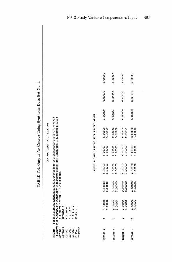
TA

BL

EF

A.

Ou

tpu

tfo

rG

enov

aU

sing

Sy

nth

etic

Dat

aS

etN

o.

4

CONT

ROL

CARD

INPU

TL

IST

ING

CO

LUH

N11

111

1111

1222

222

2222

333

333

3333

4444

4444

4455

555

5555

5666

6666

6667

7777

7777

78

1234

5678

9012

3456

7890

1234

5678

9012

345

6789

0123

456

7890

1234

5678

9012

3456

7890

1234

5678

90G

STU

DY

PX

(R:T

)D

ESI

GN--

RAND

OH

HOD

ELOP

TIO

NSRE

CORD

S2

EFFE

CT

•P

100

EFF

ECT

+T

30

EFFE

CT

+R

:T4

0FO

RMAT

(12F

2.0

)PR

OCE

SS

INPU

TRE

COR

DL

IST

ING

WIT

HRE

CORD

HEA

NS

REC

ORD

#1

5.0

0000

6.00

000

5.0

0000

5.0

0000

5.0

0000

3.0

0000

4.0

00

00

5.0

0000

6.0

0000

7.0

0000

3.0

00

00

3.0

00

00

4.7

50

00

REC

ORD

#2

9.0

0000

3.0

0000

7.0

0000

7.0

0000

7.0

0000

5.0

00

00

5.0

0000

5.0

0000

7.0

0000

7.0

0000

5.0

00

00

2.0

0000

5.7

5000

REC

ORD

#9

9.0

00

00

9.0

0000

8.0

0000

8.0

0000

6.0

0000

6.0

0000

6.0

00

005

.000

005

.00

00

08

.000

001.

0000

01

.00

00

06

.00

000

REC

ORD

#10

4.0

0000

4.0

0000

4.0

00

00

3.0

0000

3.0

0000

5.0

0000

6.0

0000

5.0

00

00

5.0

0000

7.0

0000

1.0

00

00

1.0

0000

4.0

0000

'Tl

Co o Cf)

e-e-

I:: 0­

'< ~ .... ~r ()

(l) Q o S '0 o ::l (l) ~ tn ~ .....

.::l '0 I:: e-

e .... 0'>

W

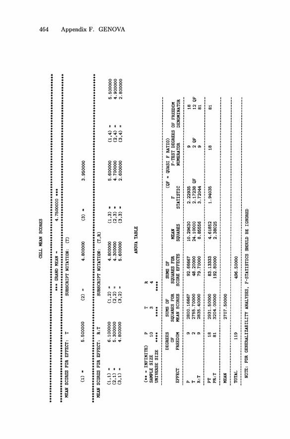
CELL

HEAN

SCOR

ES"""0) """

••••

••••

•**•

••••

••••

••••

••••

•**•

••••

**••

••••

••••

••••

**.*

*•••

•***

***

**

***

••**

**.*

*•••

••••

••••

••••

••••

••••

••••

••••

••••

••••

•••*

*•••

**

••••

••••

••••

••••

••••

••••

••••

••••

••••

••••

•**•

••••

••••

••••

••••

••••

••••

••••

••••

••••

••••

••••

**••

••••

••••

••••

••••

••••

••••

••**

*•••

****

*.

**

*.*

**

.**

•••

•••

••

••

•••

••••

••••••*•

••••

••••

••••

**••

••••

••••

•**•

••**

••**

••**

••••

***•

••••

••••

••••

••••

••••

••••

••••

••••

••••

••••

••••

•••

(1,1

)=

6.10

0000

(1,2

)=

4.8

000

00(1

,3)

•5

.600

000

(1,4

)•

5.5

0000

0(2

,1)

•5

.300

000

(2,2

)•

4.3

0000

0(2

,3)

•4

.700

000

(2.4

)•

4.9

0000

0(3

,1)

•4

.800

000

(3,2

)•

5.6

0000

0(3

.3)

•2.

6000

00(3

.4)

•2.

8000

00

ANOV

ATA

BLE

(..

=IN

FIN

ITE)

PT

RSA

MPL

ES

IZE

103

4U

NIV

ERSE

SIZ

E.*

.*••

••••

••

MEA

NSC

ORE

SFO

REF

FEC

T:

T~ "0 "0 ~ >< ~ C

)t':

lZ o ~

3.9

5000

0(3

)•

4.7

5000

00..

.

4.8

0000

0

...

GRAN

DHE

AN=

SUB

SCR

IPT

NOTA

TION

:(T

)

(2)

•

SUB

SCR

IPT

NOTA

TION

:(T

,R)

5.5

000

00(1

)•

MEA

NSC

ORE

SFO

REF

FECT

:R

:T

(QF

=Q

UA

SIF

RATI

O)

F-T

EST

DEG

REES

OFFR

EEDO

MNU

MER

ATOR

OENO

MIN

ATOR

FST

ATI

STIC

MEA

NSQ

UARE

S

SUM

SOF

SQUA

RES

FOR

SCOR

EEF

FECT

S

SUM

SOF

SQU

ARE

SFO

RHE

ANSC

ORE

S

DEG

REES

OFFR

EED

OMEF

FECT

P T R:T

9 2 9

2800

.166

6727

55.7

0000

2835

.400

00

92.6

6667

48.2

0000

79.7

0000

10.2

9630

24.1

0000

8.85

556

2.2

2935

2.1

7238

QF3

.720

44

9 2QF

9

18 12QF

81

PT PR:T

18 8129

31.5

0000

3204

.000

0083

.133

3319

2.80

000

4.6

1852

2.3

8025

1.94

035

1881

HEAN

2707

.500

00

TOTA

L1

19

496

.500

00

NOTE

:FO

RG

ENER

ALI

ZAB

ILIT

YAN

ALYS

ES,

F-ST

AT

IST

ICS

SHOU

LOB

EIG

NOR

ED

GS1

1JDY

RESU

LTS

(**

mIN

FIN

ITE

)P

SAM

PLE

SIZ

E10

UN

IVER

SESI

ZE

****

T 3*.

*.

R 4

***

*QF

H=

QUAD

RATI

CFO

RM

MO

DE

LV

AR

IAN

CE

CO

MP

ON

EN

TS

EFFE

CT

DEG

REES

OFFR

EEDO

MU

SIN

GA

LGO

RITI

lHU

SIN

GEH

SEQ

UAT

IONS

STAN

DARD

ERRO

R

VARI

ANC

E-

COVA

RIAN

CEM

ATRI

XFO

RES

TIH

ATE

DV

ARI

AN

CECO

MPO

NENT

S(V

)

NOTE

:TH

E"A

LGOR

ITIlH

"AN

D"E

HS"

ESTI

HA

TED

VARI

ANCE

COM

PONE

NTS

WIL

LBE

IDEN

TIC

AL

IFTH

ERE

ARE

NON

EGA

TIV

EES

TIH

ATE

S

EXPE

CTED

MEA

NSQ

UARE

EQU

ATI

ON

S

1.00

*VC

(PR

:T)

+4

.00*

VC

(PT

)+

12.0

0*VC

(P)

-1.

00*V

C(P

R:T

)+

4.0

0*V

C(P

T)

+1

0.0

0*VC

(R:T

)+

40.0

0*V

C(T

)1.

00*V

C(P

R:T

)+

10.0

0*V

C(R

:T)

m1.

00*V

C(P

R:T

)+

4.0

0*V

C(P

T)=

1.00

*VC

(PR

:T)

'""l

00 o tr:

e-e-

~ Po.

'< ~ .... ~T g ~ S '0 o ::l ~

0.3

766

291

0.3

6948

60

0.3

8557

580.

4379

875

0.3

7940

56

0.5

5956

792

.380

2469

0.4

7314

810

.325

1543

0.6

4753

09

0.5

595

679

2.3

8024

69

0.4

7314

810.

3251

543

0.6

4753

09

9 2 9 18 81

P T R:T

PT PR:T

EMS(

P)EH

S(T)

EHS(

R:T

)EH

S(PT

)EH

S(P

R:T

)

PT

R:T

PTPR

:T

P0

.148

6687

T0

.004

4439

0.19

183

31R

:T0

.000

0000

-0.0

359

871

0.1

4394

86PT

-0.0

444

390

-0.0

1418

490.

003

4130

0.1

4184

95PR

:T0

.000

0000

0.0

0341

30-0

.013

6520

-0.0

3413

000

.136

5199

~ -::l '0 ~ e-t-

01:0­~ c:.

n

****

****

**••

••••

••*•

•••*

••••

••*•

•**•

••••

•*

*.*

.*.*

••••

••••

•••*

***.

****

*OU

TPU

TFO

RD

STU

DIE

SW

ITH

1,2,

AND

3IT

EHS

NOT

INCL

UDED

HER

E***

**.*

****

**••

**.*

*.**

.**.

****

***

*.**

****

****

****

***

**•

••••

••**

.***

**

,;:.

0)

0)

VARI

ANCE

COHP

ONEN

TSIN

TERM

SOF

GST

UDY

UN

IVER

SE(O

FA

DH

ISSI

BLE

OBS

ERV

ATI

ON

S)SI

ZES

DST

UDY

DES

IGN

NUHB

ER0

01

-00

4

FACE

TSG

STUD

YU

NIV

ERSE

SIZ

ESD

STUD

YUN

IVER

SESI

ZES

DST

UDY

SAHP

LESI

ZES

OBJ

ECT

OFHE

ASUR

EHEN

TG

STUD

YPO

PULA

TIO

NSI

ZE

DST

UDY

POPU

LATI

ON

SIZ

ED

STUD

YSA

HPL

ESI

ZE

> '0 '0 Cl> ::s 0..

>('

~ o t':l

Z o ~ST

ANDA

RDER

RORS

VARI

ANCE

COHP

ONEN

TSFO

RHE

ANSC

ORE

S

ESTI

HA

TES

FIN

ITE

DST

UDY

UN

IVER

SESA

HPL

ING

COR-

FRE

-RE

CTIO

NS

QU

ENCI

ES

R:T

INFI

NIT

EIN

FIN

ITE

4 VARI

ANCE

COHP

ONEN

TSIN

TERM

SOF

DST

UDY

UN

IVER

SE(O

FG

ENER

ALI

ZATI

ON

)SI

ZE

S

VARI

ANCE

COHP

ONEN

TSFO

RSI

NG

LEOB

SERV

ATIO

NS

TIN

FIN

ITE

INFI

NIT

E3

STAN

DARD

ERRO

RS

VARI

ANCE

COHP

ONEN

TSFO

RHE

ANSC

ORES

ESTI

HA

TES

PIN

FIN

ITE

INFI

NIT

E10

FIN

ITE

DST

UDY

UN

IVER

SESA

HPL

ING

COR-

FRE

-RE

CTIO

NS

QU

ENCI

ES

VARI

ANCE

COHP

ONEN

TSFO

RSI

NG

LEOB

SERV

ATIO

NSE

FFEC

T

P0

.473

151

.00

00

10

.473

150

.385

580

.473

151

.00

00

10

.473

150

.38

55

8T

0.3

2515

1.0

00

03

0.1

0838

0.1

4600

0.3

2515

1.0

00

03

0.1

08

38

0.1

4600

R:T

0.6

4753

1.0

00

012

0.0

5396

0.0

3162

0.6

4753

1.0

00

012

0.0

5396

0.0

31

62PT

0.5

5957

1.0

00

03

0.1

8652

0.1

2554

0.5

5957

1.0

00

03

0.1

86

52

0.1

25

54

PR:T

2.3

8025

1.0

000

120

.198

350

.030

792

.380

251

.00

00

120

.198

350

.03

07

9

QFH

•QU

ADRA

TIC

FORM

STAN

DARD

STAN

DARD

ERRO

ROF

VARI

ANCE

DEV

IATI

ON

VARI

ANCE

UN

IVER

SESC

ORE

0.4

7315

0.6

8786

EXPE

CTED

OBSE

RVED

SCOR

E0

.858

02

0.9

263

0LO

WER

CASE

DELT

A0

.38

488

0.6

203

8U

PPER

CASE

DELT

A0

.54

722

0.7

3974

HEAN

0.2

48

15

0.4

9814

0.3

8558

0.3

65

86

0.1

2171

0.17

935

GENE

RALI

ZABI

LITY

CO

EFFI

CIE

NT

=0

.55

14

4(

1.2

293

5)

PHI

=0

.46

37

0(

0.8

6464

)

NOTE

:SI

GN

AL-

NO

ISE

RATl

OS

ARE

INPA

RENT

HESE

S

****

****

****

****

****

****

****

****

****

****

****

****

****

****

****

****

***

***O

UTP

UT

FOR

DST

UD

IES

WIT

H1,

2,AN

D3

ITEM

SNO

TIN

CLUD

EDH

ERE*

****

****

****

****

****

****

****

****

****

****

****

****

****

****

****

****

****

*

DST

UDY

DES

IGN

NUM

BER

00

2-0

04

OBJ

ECT

OFM

EASU

REM

ENT

GST

UDY

POPU

LATI

ON

SIZ

ED

STUD

YPO

PULA

TIO

NSI

ZE

DST

UDY

SAM

PLE

SIZ

E

PIN

FIN

ITE

INFI

NIT

E10

FACE

TSG

STUD

YU

NIV

ERSE

SIZE

SD

STUD

YUN

IVER

SESI

ZES

DST

UDY

SAHP

LESI

ZES

T:P

INFI

NIT

EIN

FIN

ITE

3

R:T

:PIN

FIN

ITE

INFI

NIT

E4

VARI

ANCE

COM

PONE

NTS

INTE

RMS

OFG

STUD

YU

NIV

ERSE

(OF

AD

MIS

SIBL

EOB

SERV

ATIO

NS)

SIZE

S

STAN

DARD

STAN

DARD

ERRO

ROF

VARI

ANCE

DEV

IATI

ON

VARI

ANCE

UN

IVER

SESC

ORE

0.4

7315

0.6

8786

EXPE

CTED

OBSE

RVED

SCOR

E1

.020

371

.010

13LO

WER

CASE

DELT

A0

.547

220

.739

74U

PPER

CASE

DELT

A0

.54

72

20

.739

74HE

AN0

.102

040

.319

43

QFH

=QU

ADRA

TIC

FORM

~ ......

::s "C C e-e-

~ 00 Q r:n e-e c ~ ~ ... ~r s Q o S "C o ::s ~ fJ

J

0.3

85

58

0.1

8418

0.0

4193

STAN

DARD

ERRO

RS

0.8

64

64

)0

.86

46

4)

VARI

ANCE

COM

PONE

NTS

FOR

HEAN

SCOR

ES

0.4

73

15

0.2

9491

0.2

52

31

ESTl

HA

TES

0.4

6370

0.4

6370

1 3 12

1.0

00

01

.00

00

1.0

00

0

FIN

ITE

DST

UDY

UN

IVER

SESA

MPL

ING

COR-

FRE-

RECT

ION

SQ

UEN

CIES

VARI

ANCE

COM

PONE

NTS

INTE

RMS

OFD

STUD

YU

NIV

ERSE

(OF

GEN

ERA

LIZA

TIO

N)

SIZ

ES

0.4

73

15

0.8

84

72

3.0

2778

VARI

ANCE

COHP

ONEN

TSFO

RSI

NG

LEO

BSER

VA

TIO

NS

GEN

ERA

LIZA

BILI

TYC

OEF

FIC

IEN

TPH

I

0.3

85

58

0.1

8418

0.0

4193

STAN

DARD

ERRO

RS

0.3

85

58

0.3

9265

0.1

79

35

0.1

7935

VARI

ANCE

COHP

ONEN

TSFO

RHE

ANSC

ORES

0.4

7315

0.2

9491

0.25

231

ESTI

HA

TES

1 3 12

1.0

00

01

.00

00

1.0

00

0

FIN

ITE

DST

UDY

UN

IVER

SESA

HPL

ING

COR-

FRE-

RECT

ION

SQ

UEN

CIES

0.4

73

15

0.8

8472

3.0

2778

VARI

ANCE

COM

PONE

NTS

FOR

SIN

GLE

OBSE

RVAT

IONS

EFFE

CT

P T:P

R:T

:P

NOTE

:SI

GN

AL-

ND

ISE

RATl

OS

ARE

INPA

RENT

HESE

S>I:

>­0> --

J

••••

*••*

*.**

****

****

****

****

****

****

****

••*

**

*.*

**

*.*

••••

••••

••••

••**

*OU

TPU

TFO

RD

STU

DIE

SW

ITH

1,2,

AND

3IT

EHS

NOT

INCL

UDED

HER

E***

••••

••••

••••

••••

••••

••••

••••

•••*

****

*••

•*••

••••

••••

••••

••••

*•••

••••

~ 0)

00

VARI

ANCE

COHP

ONEN

TSIN

TERM

SOF

GST

UDY

UN

IVER

SE(O

FA

DH

ISSI

BLE

OBS

ERV

ATI

ON

S)SI

ZES

DST

UDY

DES

IGN

NUHB

ER00

3-00

4

VARI

ANCE

COHP

ONEN

TSIN

TERM

SOF

DST

UOY

UN

IVER

SE(O

FG

ENER

ALl

ZATI

ON

)SI

ZE

S

FACE

TSG

STUD

YU

NIV

ERSE

SIZE

SD

STUD

YU

NIV

ERSE

SIZE

SD

STUD

YSA

HPL

ESI

ZES

~ "0 "0 (1) 8­ ><' ~ o I:':l

Z o ~ST

ANDA

RDER

RORS

VA

RIA

NCE

COHP

ONEN

TSFO

RHE

ANSC

ORE

S

ESTI

KA

TES

FIN

ITE

DST

UDY

UN

IVER

SESA

HPL

ING

COR-

FRE

-RE

CTIO

NS

QU

ENCI

ES

R:T

INFI

NIT

EIN

FIN

ITE

4

VA

RIA

NCE

COHP

ONEN

TSFO

RSI

NG

LEO

BSER

VA

TIO

NS

TIN

FIN

ITE

3 3

STAN

DARD

ERRO

RS

VARI

ANCE

COHP

ONEN

TSFO

RHE

ANSC

ORES

ESTI

KA

TES

PIN

FIN

ITE

INFI

NIT

E10

FIN

ITE

DST

UDY

UN

IVER

SESA

HPL

ING

COR-

FRE

-RE

CTIO

NS

QU

ENCI

ES

VARI

ANCE

COHP

ONEN

TSFO

RSI

NG

LE08

SERV

ATI

ON

S

OBJ

ECT

OFHE

ASUR

EHEN

TG

STUD

YPO

PULA

TIO

NSI

ZE

DST

UDY

POPU

LATI

ON

SIZ

ED

STUD

YSA

HPL

ESI

ZE

EFFE

CT

P0.

4731

51.

0000

10.

4731

50

.385

580

.659

671.

0000

10.

6596

70

.367

16T

0.3

2515

1.00

003

0.1

0838

0.14

600

0.3

2515

QFH

0.0

000

3R

:T0.

6475

31.

0000

120

.053

960.

0316

20

.647

531.

0000

120.

0539

60.

0316

2PT

0.55

957

1.00

003

0.1

8652

0.12

554

0.5

5957

0.0

000

3PR

:T2.

3802

51.

0000

120.

1983

50.

0307

92.

3802

51.

0000

120

.198

350.

0307

9

QFH

aQU

ADRA

TIC

FORM

STAN

DARD

STAN

DARD

ERRO

ROF

VA

RIA

NCE

DEV

IATI

ON

VARI

ANCE

UN

IVER

SESC

ORE

0.6

5967

0.81

220

EXPE

CTED

OBSE

RVED

SCOR

E0

.858

020

.926

30LO

WER

CASE

DELT

A0

.198

350

.445

37U

PPER

CASE

DELT

A0

.252

310

.502

31HE

AN0

.139

760.

3738

5

0.36

716

0.36

586

0.0

3079

0.0

4193

GEN

ERA

LIZA

BIL

ITY

CO

EFFI

CIE

NT

=0

.768

82PH

I=

0.72

333

3.3

2573

)2.

6144

8)

NO

TE:

SIG

NA

L-N

OIS

ERA

TlO

SAR

EIN

PARE

NTH

ESES

SUM

MAR

YOF

DST

UDY

RESU

LTS

FOR

SET

OF

CONT

ROL

CARD

SNO

.00

1

VA

RI

AN

CE

SSA

HPL

ESI

ZES

DST

UDY

----

----

----

----

----

----

----

----

----

-D

ESIG

NIN

DEX

=$P

TR

NOU

NIV

.=IN

F.

INF

.IN

F.

EXPE

CTED

UN

IVER

SEO

BSER

VED

SCO

RESC

ORE

LOW

ERCA

SED

ELTA

UPP

ERCA

SEDE

LTA

MEA

NG

EN.

COEF

.PH

I

----

----

----

----

----

----

----

----

----

----

----

----

----

----

----

----

----

----

----

----

----

----

----

----

----

----

----

----

----

----

---

003-

001

103

10.

6596

71

.45

309

0.7

9342

1.00

926

0.3

6115

0.4

5398

0.3

9527

003-

002

103

20

.659

671.

0563

80

.396

710

.504

630.

2135

60

.624

460

.566

5800

3-00

310

33

0.6

596

70

.924

140

.264

470

.336

420

.164

360

.713

820

.662

2600

3-00

410

34

0.6

5967

0.8

5802

0.1

983

50.

2523

10

.139

760

.768

820

.723

33

002-

001

103

10

.47

315

1.77

731

1.30

417

1.30

417

0.1

7773

0.2

6622

0.26

622

002-

002

103

20

.47

31

51

.272

690

.799

540

.799

540

.127

270

.371

770

.37

177

002-

003

103

30

.473

151

.104

480

.631

330

.631

330

.110

450

.428

390

.428

3900

2-0

04

103

40

.473

151.

0203

70

.547

220

.547

220

.102

040

.463

700

.463

70

SUM

MAR

YOF

DST

UDY

RESU

LTS

FOR

SET

OFCO

NTRO

LCA

RDS

NO.

003

001-

001

103

10

.473

151.

4530

90

.979

941.

3041

70

.469

540

.325

620

.266

2200

1-00

210

32

0.4

7315

1.05

638

0.5

8323

0.7

9954

0.3

2194

0.4

4790

0.3

7177

001-

003

103

30

.47

31

50

.924

140

.450

990

.631

330

.272

750

.511

990

.428

3900

1-00

410

34

0.4

7315

0.8

5802

0.3

8488

0.5

4722

0.24

815

0.5

5144

0.4

6370

SUM

MAR

YOF

DST

UDY

RESU

LTS

FOR

SET

OF

CONT

ROL

CARD

SNO

.00

2

VA

RI

AN

CE

S

~ "'"0>

CO

':j

00 o Cf)

e-e .: p..

'< ~ .... ~.

o co o o 3 "0 o = co ;:;. CI) .....

. = "0 .: e-e-

PHI

PHI

GEN

.CO

EF.

GEN

.CO

EF.

MEA

N

MEA

N

UPP

ERCA

SED

ELTA

UPP

ERCA

SED

ELTA

LOW

ERCA

SED

ELTA

LOW

ERCA

SED

ELTA

VA

RI

AN

CE

S

EXPE

CTED

UN

IVER

SEOB

SERV

EDSC

ORE

SCO

RE

EXPE

CTED

UNIV

ERSE

OBS

ERV

EDSC

ORE

SCO

RE

SAM

PLE

SIZ

ES

DST

UDY

----

----

----

----

----

----

----

----

----

-D

ESIG

NIN

DEX

=$P

TR

NOU

NIV

.=IN

F.

3IN

F.

SAH

PLE

SIZ

ES

DST

UDY

----

----

----

----

----

----

----

----

----

-D

ESIG

NIN

DEX

=$P

TR

NOU

NIV

.=IN

F.

INF.

INF

.

Appendix GurGENOVA

urGENOVA (Brennan, 2001b) is an ANSI C computer program for estimat­ing random effects variance components for both balanced and unbalanceddesigns that are complete in the sense that all interactions are included.urGENOVA was created primarily for designs that are unbalanced withrespect to nesting and that contain single observations per cell, However,for designs that are not "too large," urGENOVA can also estimate randomeffects varian ce components when some cells are empty and/or the numbersof observations within cells are unequal.

Random effects variance components are estimated by urGENOVA us­ing the analogous-ANOVA pracedure discussed in Section 7.1.1, which issometimes called Henderson 's (1953) Method 1. The algorithms used donot require operations with large matrices . For designs (balanced or un­balanced) with single observations per cell, urGENOVA can process verylarge data sets in a relatively short amount of time. urGENOVA extendsGENOVA (see Appendix F) in the sense that urGENOVA can handle un­balanced designs, as weIl as all the balanced designs that GENOVA canprocess. However, urGENOVA has no D study capabilities.!

Input to urGENOVA consists of a set of contral cards and an input dataset. The urGENOVA contral cards have an appearance similar to thosefor GENOVA, and both programs require that effects be identified in themanner discussed in Section 3.2.1. However, the control card conventions

1Für some unbalanced designs , mGENOVA can be used to obtain D study results(see Appendix H).

472 Appendix G. urGENOVA

for the two programs are not identical. Also, the urGENOVA rules forformatting and ordering records for the input data set are not quite asflexible as the rules for GENOVA.

Output for urGENOVA that is always provided includes:

• a listing of the control cards;

• means for main effects; and

• an ANOVAtable with degrees of freedom, uncorrected sums of squares(T terms), sums of squares , mean squares , and estimated random ef­fects variance components.

Optional output includes:

• a list of some or all of the input data records;

• expected values of T terms ;

• expected mean squares;

• for balanced designs only , estimated standard errors; and

• for balanced designs only, both Satterthwaite confidence intervals (seeSection 6.2.2) and Ting et al. confidence intervals (see Section 6.2.3)for estimated variance components using a user-specified confidencecoefficient.

urGENOVA and program documentation can be obtained from the au­thor (robert-brennan@uiowa.edu) or from the Iowa Testing Programs Website (www .uiowa.eduy Ttp}. At this time, both PC and Macintosh versionsof urGENOVA are available free of charge.

Appendix HmGENOVA

mGENOVA (Brennan, 2001b) is an ANSI C computer program for per­forming multivariate generalizability G and D studies for a set of designsthat may be balanced or unbalanced with respect to nesting. Specifically,mGENOVA can be used with all of the G study designs in Table 9.2 [ex­cept the (po :c·) x iO design] and their D study counterparts. These arecalled "canonical" designs here. For these designs, with minor exceptions,mGENOVA can perform all ofthe computations discussed in Chapters 9 to12. The algorithms used do not require operations with large matrices, andmGENOVA can process very large data sets in a relatively short amountof time .

When nv = 1, the canonical G study designs are simply p x i , i :p,p x i x h, p x (i :h) , and (p :c) xi. For any one of these designs and itsD study counterpart, mGENOVA provides output comparable to that ofGENOVA (see Appendix F) when the design is balanced. When the designis unbalanced, the G study output is comparable to that of urGENOVA(see Appendix G) and , in addition, mGENOVA provides D study output .

Input to mGENOVA consists of a set of control cards and usually an in­put data set . The control card setups and input data conventions are verysimilar to those for urGENOVA and quite similar to those for GENOVA.The mGENOVA rules for formatting and ordering records for the inputdata set are very much like those of urGENOVA. G study estimated vari­ance and covariance components can be used as input to obtain D studyresults.

When designs are balanced, estimates of variance and covariance compo­nents based on mean squares and mean products, respectively, have certain

474 App endix H. mGENOVA

desirable statistical properties. When designs are unbalanced with respectto nest ing, however, there is usually no compelling statistical argument forusing analogous mean squares (or analogous T terms; see Section 7.1.1) andanalogous mean products (or analogous TP terms; see Section 11.1.2) forestimation. As options, mGENOVA permits the use of C terms to est imatevariance components and CP terms to estimate covariance components, asdiscussed in Section 11.1.3.

G st udy output (some of which is optional) includes:

• a listing of the control cards;

• a list of some or all of the input data records;

• means for most main effects ;

• statistics used to estimate G study varian ce and covariance compo­nents; and

• G st udy est imated variance and covariance components.

D st udy out put (some of which is opt ional) includes:

• est imated variance and covariance components;

• est imated universe score matrix and error matrices;

• results for each level of the fixed facet Vj

• results for a user-defined composite, based on w and /or a weights asdiscussed in Sections 10.1.3 and 10.1.5, respectively;

• conditional st andard errors of measurement for the composite ; and

• result s relating to regressed score estimates for profiles and compos­ites.

mGENOVA and program documentation can be obtained from the au­thor (robert-brennan@uiowa.edu) or from the Iowa Testing Programs Website (www.uiowa.eduy'Ttp). At thi s time, both pe and Macintosh versionsof mGENOVA are available free of charge.

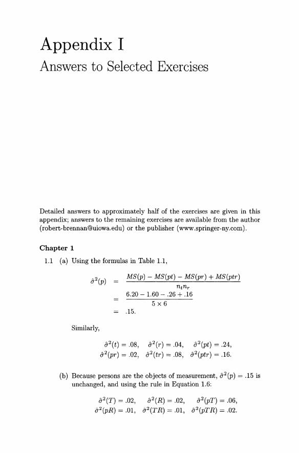
Appendix IAnswers to Selected Exercises

Detailed answers to approximately half of the exercises are given in thisappendix; answers to the remaining exercises are available from the author(robert-brennan@uiowa.edu) or the publisher (www.springer-ny.com).

Chapter 1

1.1 (a) Using the formulas in Table 1.1,

MS(p) - MS(pt) - MS(pr) + MS(ptr)ntnr

6.20 - 1.60 - .26 + .16

5 x6.15.

Similarly,

o-2(t) = .08, o-2(r) = .04, o-2(pt) = .24,

o-2(pr) = .02, o-2(tr) = .08, o-2(ptr) = .16.

(b) Because persons are the objects of measurement , o-2(p) = .15 isunchanged, and using the rule in Equation 1.6:

o-2(T) = .02, o-2(R) = .02, o-2(pT) = .06,

o-2(pR) = .01, fj2(TR) = .01, fj2(pTR) = .02.

476 Appendix 1. Answers to Selected Exercises

(c) Absolute error variance: From the "T, R random" coIumn ofTable 1.2,

a2 (L\) = a2 (T ) + a2 (R) + a2 (pT )

+a2 (pR) + a2 (T R) + a2 (pT R)

= .02+ .02+ .06+ .01 + .01 + .02 = .14.

Relative error variance: From the "T, R random" coIumn of Ta­ble 1.2,

a2 (0) = a2 (pT ) + a2 (pR ) + a2 (pT R) = .06 + .01 + .02 = .09.

Generalizability coefficient: From Equation 1.12, when T and Rare both random, a2 (r ) = a2 (p) and

.15 = .63..15 + .09

Index 0/ dependability: From Equation 1.13, since a2 (r ) = a2(p)when T and Rare both random,

(d) First , we need to estimate G study variance components forthe p x (r: t) design given the results in (a) for the p x t x rdesign. Under these circumstances, a2 (p) = .15, a2 (t ) = .08,and a2 (pt ) = .24 are unchanged. Using Equation 1.15,

a2(r:t ) = a2(r ) + a2(tr ) = .04 + .08 = .12,

and using Equation 1.16

a2 (pr:t) = a2 (pr ) + a2 (ptr ) = .02 + .16 = .18.

Second, using the rule in Equation 1.6, for n~ = 3 and n~ = 2,the estimated random effects D study variance components are:

a2 (p) = .150, a2 (T ) = .027,

a2(pT ) = .080, and

a2 (R:T) = .020,

a2 (pR:T) = .030.

Third, since T and Rare random, we use the second coIumn inTable 1.3 to obtain

a2(L\) = a2 (T ) + a2 (R:T) +a2 (pT ) + a2 (pR:T)

= .027 + .020 + .080 + .030 = .157.

The square root is a(L\) = .40.

Appendix 1. Answers to Selected Exercises 477

1.2 If there are only two facets and both facets are considered fixed, thenevery instance of a measurement procedure would involve the samecondit ions. Under th ese circumstances , th ere is no generalizat ion to abroader universe of condit ions of measurement . Logically, therefore,all error variances are zero, by definition. No measurement procedureis that precise! To avoid this problem, at least one of the facets in auniverse of generalizat ion must be viewed as variable across inst ancesof the measurement procedure.

Chapter 2

2.1 (a) The ANOVA table is

Effect( O') df (0') 88(0') M8(0') 0-2(0')

P 5 81.3333 16.2667 5.0000r 2 12.0000 6.0000 .7889pr 10 12.6667 1.2667 1.2667

(b) 0-2(8) = .4222, 0-2 (ß ) = .6852, E ß2 = .922, and ~ = .879.

(c) In terms of covariances

2(4.0 + 3.6 + 7.4) = 56 '

which is ident ical to the est imate of universe score variance based onmean squares.

2.3 Starting with Equ ation 2.37,

EE(Xp/ - /-l )2P I

E E(vp + VI + VPI) 2P I

= E v~ + E VJ + E E v~1P I P I

a2(p ) + a2(I ) + a2(P I)

a2(p) a2(i ) a2(pi )- - + - -+--.n' n' n'n'p t p t

2.5 It is easier to solve this problem using estimates of signal-noise ratiosthan generalizability coefficients. Specifically, for Math Concepts,

_ _.0_28_0_ __.6_ -15, 2:: - . ,.1783/ n i 1 - .6

which implies that n~ 2:: 9.5. Similarly, for Estimation,

.0242 .6 _ 5- - - >---1. ,. 1 994/n~ - 1 - .6

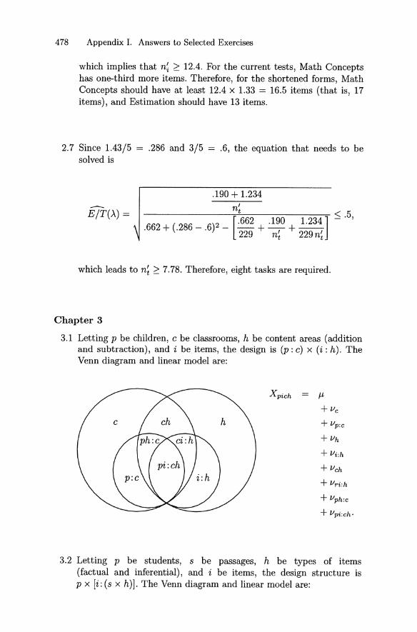
478 Appendix 1. Answers to Selected Exercises

which implies that n~ 2: 12.4. For the current tests , Math Conceptshas one-third more items. Therefore, for the shortened forms, MathConcepts should have at least 12.4 x 1.33 = 16.5 items (that is, 17items), and Estimation should have 13 items.

2.7 Since 1.43/5 = .286 and 3/5solved is

.6, the equation that needs to be

--E/T()") =

.190 + 1.234n't

.662 (.286 _ .6)2 _ [.662 .190 1.234]+ 229 + n~ + 229n~

which leads to n~ 2: 7.78. Therefore, eight tasks are required.

Chapter 3

3.1 Letting p be children, c be classrooms, h be content areas (addit ionand subtraction), and i be items, the design is (p :c) x (i : h). TheVenn diagram and linear model are:

X pich /L

+ V«

+ vp :c

+Vh

+ Vi :h

+ Vch

+ Vr i :h

+ Vph :c

+ Vpi .ch »

3.2 Letting p be students , s be passages, h be types of items(factual and inferential) , and i be items, the design st ructure isp x [i : (s x h)]. The Venn diagram and linear model are:

Appendix 1. Answers to Selected Exercises 479

Xpish = JL

+vp

+ Vs

+Vh

+ vsh

+ vi:sh

+ Vp«

+ Vph

+ Vpsh

+ Vpi :sh·

Most likely, the universe of admissible observations is i: (s x h) withNi --+ 00, N, --+ 00, and Ni, = 2.

3.4 For a-2 (p) in this design, 11"(&) = ninh, and Aconsists of the index h,only, because ph is the only component that contains p and exactlyone additional index. Therefore, Step 1 results in subtracting onlyMS(ph) from MS(p) , and the estimator is

a-2 (p) = MS(p) - MS(ph).ninh

For a-2 (h), 11"(&) = npni, and A consists of the indices p and i becauseboth ph and i:h contain hand exactly one additional index . There­fore, Step 1 results in subtracting MS(ph) and MS(i :h) from MS(h) .Step 2 results in adding MS(pih) . The resulting estimator is:

a-2(h) = MS(h) - MS(ph) - MS(i :h) + MS(pih) .npni

480 Appendix 1. Answers to Selected Exercises

3.5

(p:c:t) X i Design

X pi ct = M

+ Vt

+ Vc .t.

+ vp:c :t

+ Vi

+ Vti

+ Vci:t

+ Vp i :c:t·

Effect(a) df(a) T(a) SS(a) MS(a)

tc:tp:c:titici:tpi:c:tMean (M)

4142

109210

410420

10920

83000.764084070.525090521.849081147.292884086.746885558.006897506.452980850.0000

2150.76401069.76106451.3240297.2928788.6900401.4990

5497.1221

52.457725.47055.9078

29.72931.92360.95590.5034

.0845

.1241

.4913

.0236

.0346

.0323

.5034

3.7 (a) The expected mean squares are :

EMS(p)

EMS(ph)

EMS(pi:h)

= (1 - ndNi)(J2(pi:hIM) + (1 - nh/Nh)ni (J2(phIM)

+ ninh (J2(pIM)

(1 - ndNi)(J2(pi:hIM) + ni (J2(phIM)

= (J2(pi :hIM).

(b) In terms of random effects variance components,

(c) For the random model variance components,

(J2(p) = EMS(p) - EMS(ph) ,ninh

(J2(ph) = EMS(ph) - EMS(pi:h)Nh niNh

Appendix I. Answers to Selected Exercises 481

and

The sum of t hese is

EMS(p) - (1 - nh/Nh)EMS(ph)

ni nh

+ (Ni~h - ni~h ) EMS(pi:h) .

Replacing the previously derived expected mean squares in the aboveequation proves the equality.

Chapter 4

4.1 In this case, the statement that score effects are uncorrelated meansthat EVphVphl = °for h f h'. It follows that

=

=

4.4 Using the confounded-effects rule , the effects in the p x (i: h) designcan be denoted:

p, h, i :h =} (i , i h), ph, and pi :h =} (pi,pih).

Similarly, the effects in th e (i x h) :p design can be denoted:

p, i :p =} (i ,pi) , h:p =} (h,ph) , and ih:p =} (ih,pih).

The i :p effect in th e (i x h) :p design involves two effects from a fullycrossed design, i and pi. There is no combination of effects in thep x (i :h) design th at gives precisely these two effect s. A similar state­ment s holds for ih:p.

However , if (J2(ih :p) = 0, then (J2 (ih ) = (J2(pih ) = °because vari­ance components are necessarily positive. In this case, (J2 (i: p) in the(i x h):p design can be obtained by combining (J2(i :h) and (J2 (pi :h)from the p x (i :h) design.

482 Appendix I. Answers to Selected Exercises

4.6 The D study results are summarized next.

D Studies

a2(a) for a2(a) for n' 1 2t

P x (r:t) r :t:p n' 12 6r

Design Design n~n~ 12 12

a2(p) = .4731 a2(p) = .4731 a2(p) .473 .473

a2(t) = .3252 } a2(t:p) = .8848 a2(T:p) .885 .442a2(pt) = .5596

~(2(r :t)) = .6475 } a2(r:t:p) = 3.0277 a2 (R:T:p) .252 .252a pr:t = 2.3802

a2(7) .47 .47a2(8) = a2 (.6.) 1.14 .69

E ß2 = ~ .29 .41

These results are ident ical to the ahsolute-error-based results in Ta­ble 4.6 for the p x (R :T ) design.

4.7 In terms of estimators, t he inequality SjN(8) ~ 2 means that

and in terms of the estimates for this examp le,

0845> 2 [. 1241 .4913 .0346 .0323 .5034 ]. - n~ + 20n~ + 11 + 11n~ + (20)( 11)n~ .

Solving this inequality gives n~ = 4.

Alternatively, this exercise can be solved by computing D st udy re­sults for different values of n~ unt il the re~red value of n~ is de­

termined~or th is example, when n~ = 3, SjN(8) = 1.58, and whenn~ = 4, SjN(8) = 2.08.

4.9 For the random model,

A(X ) J.47+ .58 ( )a = 10 + .80 - .58 = .57.

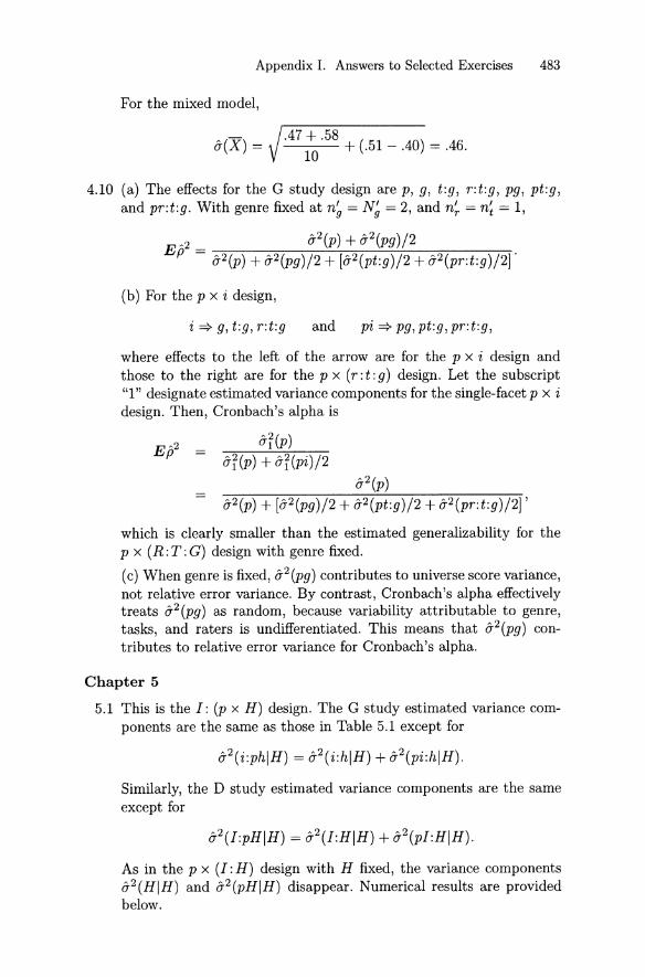
Appendix I. Answers to Selected Exercises 483

For the mixed model,

'(-) ).47 + .58 ( )(J X = 10 + .51 -.40 = .46.

4.10 (a) The effects for the G study design are p, g, t:g, r:t :g, pg, pt :g,and pr:t:g . With genre fixed at n~ = N~ = 2, and n~ = n~ = 1,

E , 2 _ 0-2(p) + 0-2(pg)/2p - 0-2(p) + 0-2(pg)/2 + [0-2(pt:g)/2 + 0-2(pr:t:g)/2]'

(b) For the p x i design,

i=? g, t:g, r:t:g and pi =? pg,pt :g,pr:t:g,

where effects to the left of the arrow are for the p x i design andthose to the right are for the p x (r: t :g) design. Let the subscript"1" designate estimated variance components for the single-facet p x idesign. Then, Cronbach's alpha is

0-2(p) + [0-2(pg)/2 + 0-2(pt:g)/2 + 0-2(pr:t:g)/2J'

which is clearly smaller than the estimated generalizability for thep x (R:T:G) design with genre fixed.

(c) When genre is fixed, 0-2(pg) contributes to universe score variance,not relative error variance . By contrast, Cronbach's alpha effectivelytreats 0-2(pg) as random, because variability attributable to genre,tasks, and raters is undifferentiated. This means that 0-2 (pg) con­tributes to relative error variance for Cronbach's alpha.

Chapter 5

5.1 This is the I : (p x H) design. The G study estimated variance com­ponents are the same as those in Table 5.1 except for

Similarly, the D study estimated variance components are the sameexcept for

As in the p x (I: H) design with H fixed, the variance components0-2(HIH) and 0-2(pHIH) disappear. Numerical results are providedbelow.

484 Appendix I. Answers to Selected Exercises

a2 (pIH ) = .0378a2(hIH ) = .0013

a2(phIH ) = .0051a2(i :phIH ) = .1848

D Study Results

a2 (pIH ) .0378a2(H IH )

a2(pH IH )a2(I :pH IH ) .0046

a2 (r ) .0378172(8) = a2 (b.) .0046

EjP = ~ .892

5.2 This is the p X (i:h) X 0 design. Using a dashed circle to representthe fixed facet h, the Venn diagram and linear model are

,\

\

\

h \

,I

I

I

I

Xpoih Jl

+vp

+ Vo

+Vh

+ Vi :h

+ vpo

+Vph

+ Vpi :h

+ Vot:

+ Voi .li

+ Vpoh

+ Vpoi :h·

Generalization for a single randomly selected occasion means thatn~ = 1 < N~ -+ 00. The G and D study results are as folIows.

Appendix 1. Answers to Selected Exercises 485

Effeet MB &2(aIH) d(älp) C(älp) &2(äIH)

p 2.9304 .0320 1 1 .03200 .6068 .0000 1 1 .0000h 18.4148 .0022 5 0i:h 10.6986 .0252 40 1 .0006po .2085 .0031 1 1 .0031ph .2767 .0006 5 0pi:h .2406 .0791 40 1 .0020oh .5290 .0002 5 0oi :h .1742 .0004 40 1 .0000poh .1089 .0033 5 0poi :h .0825 .0825 40 1 .0021

&2(7) = .0320&2(8) = .0072Eß2 = .816

5.3 In Exercise 5.6, Eß2 is for a single oeeasion that is random, whereasin Table 5.1 the single oeeasion is hidden and fixed. This differeneeis the primary reason the Eß2 in Exercise 5.6 is smaller than Eß2 inTable 5.1. The D st udy varianee eomponents in Exercise 5.6 ean beused to est imate results for a single level of a fixed, hidden oeeasionfaeet in the following manner .

&2(7) = &2(pIH) + &2(poIH) = .0320 + .0031 + .0351,

&2(8) = &2(pI:HIH) + &2 (poI: H IH ) = .0020 + .0021 = .0041,

andE 2 _ .0351 _

P - .0351 + .0041 - .895.

5.7 (a) Inequality 5.25 is not sat isfied beeause

&2(g) = .07 = .23 &2(gi) = .07 = .14.&2(g) + &2(p:g) .30 > &2(gi) + &2(pi:g) .50

(b) For np = 20 and n i = 5,

Eß~ = .70 < E ß; = .75.

Indeed, for n i = 5, E ß; < Eß~ whenever np ::; 33. Furthermore, forany value of ni 2:: 1, Eß; < Eß~ whenever np ::; 14.

5.9 Using Equation 5.32, the values of &(bo) for the six persons are: .6667,.8819, .5774, .3333, 1.2019, and 1.0000. The average of their squaredvalues is .6852, which is &2(bo) , as reported in the answer to Exer­eise 2.6 in Chapter 2.

486 Appendix 1. Answers to Selected Exercises

Chapter 6

6.1 Using Equation 6.29,

2(11.6273)2 2[9(2.7872)]211 +2 + (9)(11) +2 = .0481.

6.2 From Table 6.2, for n~ = 12, 0-2(6.) = .3059, and using df rather thandf+2 in the answer to Exercise 6.6 gives 0-[0-2(6.)] = .0509. Therefore,the ratio in Equation 6.19 is r = 6.011. Referring to Appendix D, thisratio falls between the following two rows

r

6.0006.042

Lower

.8206

.8217

Upper

1.26061.2584

Using linear interpolation gives lower-limit and upper-Iimit valuesof .8203 and 1.2603, respectively. Multiplying these limit values by0- 2(6.) = .3059 gives the interval (.251, .385).

6.5 It is easy to verify that 0-2(p) = 4.25 for the full data matrix. It isalso easy, although tedious, to determine the values of 0-2(p) for eachof the 3 x 3 x 3 = 27 possible samples of three persons taken withreplacement:

Rows 0-2(p) Rows 0-2(p) Rows 0-2(p)

1 1 1 .000 2 1 1 .167 3 1 1 5.2221 1 2 .167 2 1 2 .167 3 1 2 4.2501 1 3 5.222 2 1 3 4.250 3 1 3 5.2221 2 1 .167 2 2 1 .167 3 2 1 4.2501 2 2 .167 2 2 2 .000 3 2 2 3.4441 2 3 4.250 2 2 3 3.444 3 2 3 3.4441 3 1 5.222 2 3 1 4.250 3 3 1 5.2221 3 2 4.250 2 3 2 3.444 3 3 2 3.4441 3 3 5.222 2 3 3 3.444 3 3 3 .000

The mean of these 27 estimates is 2.833, and (3/2) x 2.833 = 4.25,which is unbiased since it is an ANOVA estimate. Ifwe want 0-2[a2(p)]to be an unbiased estimate, then the adjustment factor must be usedwith the bootstrap estimate of the standard error of 0-2(p).

6.6 For these data,

Effect

trtr

df

91199

MB

19.75003.00002.7500

4.2500.0833

2.7500

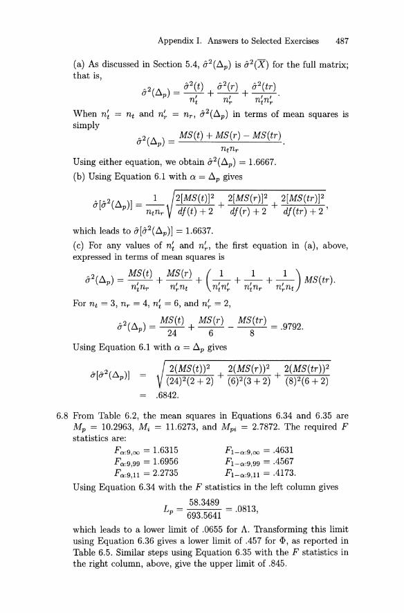
Appendix 1. Answers to Selected Exercises 487

(a) As discussed in Sect ion 5.4, a-2(~p) is a-2(X) for the full matrix;that is,

a-2(~ ) = a-2(t) + a-

2(r) + a-2(tr).

p n' n' n'n't r t r

When n~ = nt and n~ = nr , a-2(~p) in terms of mean squares issimply

a-2(~p) = MS(t) + MS(r) - MS(tr).ntnr

Using either equation, we obtain a-2(~p) = 1.6667.

(b) Using Equation 6.1 with a = ~p gives

2[MS(t)]2 2[MS(r)]2 2[MS(tr)]2df(t) + 2 + df(r) + 2 + df(tr) + 2 '

which leads to a-[a-2(~p)] = 1.6637.

(c) For any values of n~ and n~, the first equation in (a) , above,expressed in terms of mean squares is

A2( 1\ ) = MS(t) MS(r) (_1_ _1_ _1_) MS( )o U p , + , + ,,+, +, tr .ntnr nrnt ntnr ntnr nrnt

For nt = 3, nr = 4, n~ = 6, and n~ = 2,

A 2 (~ ) = MS(t) MS(r) _ MS(tr) = .9792.a p 24 + 6 8

Using Equation 6.1 with a = ~p gives

2(MS(t))2 2(MS(r))2 2(MS(tr))2(24)2(2 + 2) + (6)2(3 + 2) + (8)2(6 + 2)

.6842.

6.8 From Table 6.2, the mean squares in Equations 6.34 and 6.35 areMp = 10.2963, Mi = 11.6273, and Mpi = 2.7872. The required Fstatistics are :

Fa :9 ,oo = 1.6315 F1- a :9 ,oo = .4631Fa :9,99 = 1.6956 F1- a :9,99 = .4567Fa :9 ,1l = 2.2735 F1- a :9 ,1l = .4173.

Using Equation 6.34 with the F statistics in the left column gives

58.3489Lp = 693.5641 = .0813,

which leads to a lower limit of .0655 for A. Transforming this limitusing Equation 6.36 gives a lower limit of .457 for <1> , as reported inTable 6.5. Similar steps using Equation 6.35 with the F statistics inthe right column, above, give the upper limit of .845.

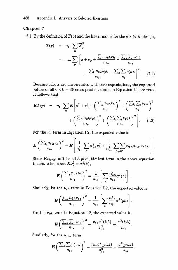
488 Appendix I. Answers to Selected Exercises

Chapter 7

7.1 By the definition ofT(p) and the linear model for the p x (i :h) design,

T(p) ni+ LX~p

" [ Lh ni:hl/h Lh L i I/i:h= ni+L...J J.L + I/p + + =c::...=::..:.-_

p ni+ ni+

+ Lh ni:hl/ph + Lh L i I/Pi:h]2 (I.1)ni+ ni+

Because effects are uncorrelated with zero expectations, the expectedvalues of all 6 x 6 = 36 cross-product terms in Equation 1.1 are zero.It follows that

ET(p) = ni+ L E [J.L2+ 1/; + (Lh ni:hl/h)2 + (Lh ~i I/i:h)

2p nH n H

+ (Lh n~:hI/Ph)2+ (Lh ~i I/Pi:h) 2]. (1.2)nH nH

For the I/h term in Equation 1.2, the expected value is

Since EI/hl/h' = 0 for all h -=I- h' , the last term in the above equationis zero. Also, since EI/~ = (J'2(h),

Similarly, for the Vpb: term in Equation 1.2, the expected value is

For the I/i:h term in Equation 1.2, the expected value is

Similarly, for the I/pi:h term,

Appendix I. Answers to Selected Exercises 489

It follows that

ET(p) = npni+p,2 + npni+a2(p) + nprw2(h)

+ npa2(i:h) + npria2(ph) + npa2(pi:h),

where r , = Eh n;:h/ni+'

7.2 Since MS(p) = [T(p) - T(p,)JI(np - 1),

EMS(p) = ET(p) - ET(p,)np -1

(np - 1)[a2(pi:h) + ria2(ph) + ni+a2(p)J=

np -1

a2(pi:h) + ria2(ph) + ni+a2(p).

Similar derivations lead to the other expected mean squares.

7.3 Straightforward algebra .

7.4 Straightforward algebra .

7.5 Straightforward algebra.

7.6 Straightforward computations.

7.7 Given the definition of X p in Equation 7.22, the expected value of-2

the sum of X p is

When the square is taken, followed by the expectation, the cross­product terms will be zero. Therefore , without loss of generality

The expected value of the last term will involve ni:p occurrences ofa2(i:p), as weIl as the expected value of ni:p(ni:p - 1) cross-productterms, all of which are zero. It follows that

490 Appendix I. Answers to Selected Exercises

where iii is the harmonie mean of the ni:p.

For the definition of X in Equation 7.22, the expeeted value of X2

is

To determine the expeeted value of the term in parentheses it ishelpful to eonsider a special ease, say two persons with two and threeitems per person. For this special ease, the expeeted value is

E ( Vl:l ; V2 :1 + V1:2 + V~:2 + V3 :2) 2

Sinee the expected value of the square of eaeh Vi :p term is (J2(i:p),and the expeeted value of eaeh eross-produet term is zero, this specialease leads to (J2(i:p)/2 + (J2(i:p)/3 . Generalizing this logic gives

Chapter 8

8.1 Straightforward eomputations.

8.2 When the p x I design is used to analyze a situation that is more eor­reetly eharaeterized as a p x (I: H) design, (j2(pH) and (j2(pI:H) forthe p x (I: H) design are eonfounded in (j2(pI) for the p x I design.Therefore, an estimate of (J2 (8) for the p x I design is

(j2(ph) + (j2(pi:h) .0098 + .1710. = 40 = .0045,n H

App endi x 1. Answers to Select ed Exercises 491

which gives EfP = .0219/(.0219 + .0045) = .830. These estimatesare questionable because they fail to distinguish between the effectsat t r ibutable to st imuli and items . In particular , the a-2 (ph) effectis divided by t he tot al number of items, rather than the numberof stimuli, which leads to an underestimate of error variance and acorresponding overest imate of reliability.

8.3 For E ß2 ~ .85, relative erro r vari an ce must be less than or equal to

[1 - E ß2] , 2 [1 - .85]

E ß2 a (p) = --:85 .0219 = .00386.

Therefore , we need values for n~ , n~+ , and the n~:h such that

(1.3)

subject to the constra int that

(l A)

Analyti c strategies and /or trial-and-error give the following results:

n' n~+ n~:hv I a-2(0) E ß2 Min .h n h

7 70 10,10,10,10,10,10,10 10.0000 .00342 .86493 49.08 65 8,8,8,8,8 ,8,8,9 7.9868 .00386 .85016 48.59 62 6,7,7,7,7,7,7,7,7 8.9813 .00385 .85049 49.0

10 60 6,6,6,6,6,6 ,6,6,6,6 10.0000 .00383 .85115 50.0

Not e t hat für six st imuli t here are no sa mple sizes that satisfy bothEquations 1.3 and 1.4 simultaneously; the same holds for 11 stimuli.

One way to obtain these results is to (a) specify some value of n~

and use it for n~ in Equ ation 1.3, which can t hen be used to get apreliminary valu e for n~+; (b) round up this value of n~+ and find the"flat test" pattern of n~ values for the n~:h that sum to n~+; (c) verifythat these sarnple sizes give Eß2 ~ .85; and (d) determine whetherthese sarnple sizes lead to a test that is no longer than 50 minutes.For example, using n~ = 8 für n~ in Equation 1.3 gives

I = a-2(pi :h) = .1710 =6490

n H a-2 (0) - [a- 2 (ph)/ 7] .00386 - (.0098/8) . ,

which mean s that we need to distribute 65 items over the eight stim­uli. The flattest distribution (Le., the one t hat leads to t he largestvalue of n~) has seven st imuli wit h eight items and one with nineitems, which gives n~ = 7.9868. We can now determine that the es­t imated generalizability coefficient is E ß2 = .85016 < .85. Für t hese

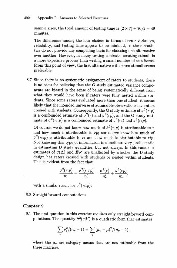
492 Appendix I. Answers to Selected Exercises

sample sizes, the total amount of testing tim e is (2 x 7) + 70/2 = 49minutes.

The differences among the four choices in terms of error variances,reliability, and testing time appear to be minimal, so these statis­tics do not provide any compelling basis for choosing one alternativeover another. However, in many testing contexts, creating stimuli isa more expensive process than writing a small number of test items.From this point of view, the first alternative with seven stimuli seemspreferable.

8.7 Since there is no systematic assignment of rat ers to st udents, thereis no basis for believing that the G study estimated variance compo­nents are biased in the sense of being systematically different fromwhat they would have been if raters were fully nested within stu­dents. Since some raters evaluated more than one student, it seemslikely that the intended universe of admissible observations has raterscrossed with students. Consequently, the G st udy estimate of a2(r:p)is a confounded estimate of a 2 (r ) and a 2 (rp), and the G st udy esti­mate of a2(ri:p) is a confounded estimate of a2(ri) and a2(rip).

Of course , we do not know how much of a2 (r:p) is attributable to rand how much is attributable to rp; nor do we know how much of(j-2( ri:p) is attributable to ri and how much is attributable to rip.Not knowing this type of information is sometimes very problematicin est imat ing D study quantities, but not always. In this case , ourestimates of a(ß) and E p2 are unaffected by whether the D studydesign has raters crossed with students or nested within students.This is evident from the fact that

with a similar result for a2(ri:p).

8.8 Straightforward computations.

Chapter 9

9.1 The first question in this exercise requires only straightforward com­putations. The quantity (j-2(vlV) is a quadratic form that estimates

v v

where the J.Lv are category means that are not estimable from thethree matrices.

Appendix 1. Answers to Selected Exercises 493

9.2

:Ep [i i]:Ei [ X

X ]=

I :Eh = [ XX ]I

P v I :Epi [ XX ]

I

:Eph [ X X ]I =

:Eih [ X X ]=

:Epih = [ XX ]

VI V2

hl h2 h3 h4 hs h6

P i l i2 i3 i4 i l i2 i3 i4 is i6 is i6 is i6 is i61 X X X X X X X X X X X X X X X X

np X X X X X X X X X X X X X X X X

9.4 Straightforward computation.

9.5 For a p. x iO design, o-vv ,(p) = Svv,(p) (see Equ ation 9.8), and it iseasy to show that

Svv,(p) = MPvv,(p)/ ni .

Therefore, t he est imated covariance component is 3.4611/6 = .5769.

9.7 o- [o-vv'(i)] = .190 and o- [o-vv' (pi)] = .227.

9.9 Recall t he general formula for t he variance of a difference:

var (X - Y ) = var(X) +var (Y) - 2cov(X ,Y ).

It follows th at

(X Y )_ var(X) + var(Y) - var(X - Y )

cov , - 2 '

494 Appendix 1. Answers to Selected Exercises

or, in the notat ional conventions of t his chapte r,

avv'(O:) = a~(o:) + 17; ,(0:) - a;_v'(O:) .2

It follows that the variance-covariance matrices are:

~p = [.0058 -.0031 ] ~h = [

.1238-.0031 .0334 ' .0519

~i:h = [.0279 .0048 ] ~ph = [

.0177.0048 .0028 ' .0035

~ [ .0432 -.0004 ]:E pi :h = -.0004 .0438 .

.0519 ]

.0298

.0035 ]

.0606

Chapter 10

10.1 T he universe score, relative erro r, and absolute error matrices are

4.2856

5.0832

11.857144.57147.5714

[ 6.2857:E T = 11.8571

2.0000

~6[ 1.1428

~ [ 2.0000:E L\

2.0000 ]7.57147.4286

.8572 ]

1.7500 ] .

For t he total score metric the w weights are all unity. The compositeuniverse score var iance , relative error var iance, and absolute errorvar iance in t he total score metri c are, respect ively, ab(T) = 101.143,ab(J) = 6.286, and ab (~) = 8.833. It is now easily verified that E ß2

and <Ii are t he same values as for t he mean score metric reportedpreviously.

10.2 Since the a priori weights are all equal, t hey can be eliminated fromEquation 10.46, which results in optimal samp le sizes of

n~ l = 10.).3444 + 1.2522 = 3.2651.).4286 + .5714 + .).1994 + 1.0714 + .).4464 + .4286 '

n~2 = 10.).1994 + 1.0714 = 3.6808.).4286 + .5714 + .).1994 + 1.0714 + .).4464 + .4286 '

and

10.).4464 + .4286 0n~3 = = 3. 542.

V.4286 + .5714 + V.1994 + 1.0714 + .).4464 + .4286

Using n~l = 3, n~2 = 4, and n~3 = 3 gives ab (~) = .105.

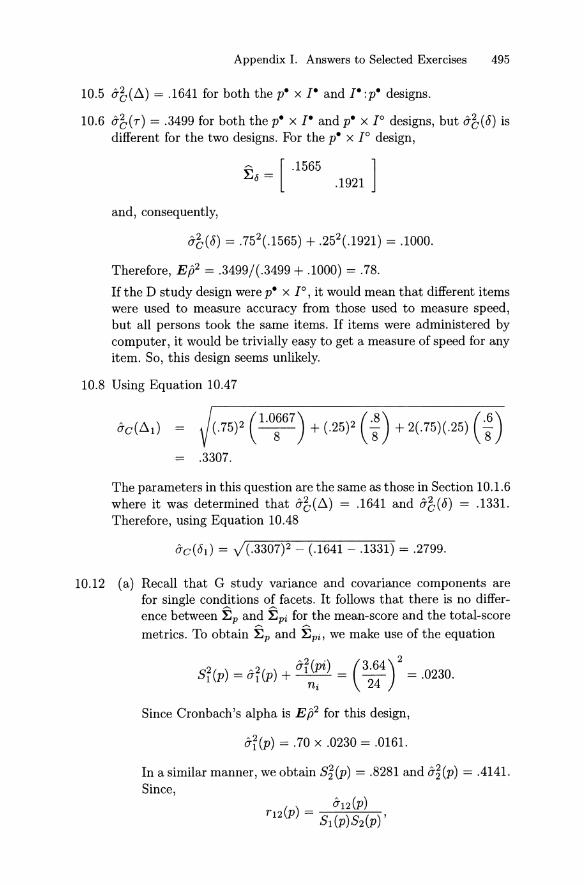
Appendix 1. Answers to Selected Exercises 495

10.5 &b(ß) = .1641 for both the p. x rand J. :p. designs.

10.6 &b(r) = .3499 for both the p. x rand p. x JO designs, but &b(<5) isdifferent for the two designs. For the p. x JO design,

}3 = [ .1565 ]8 .1921

and, consequently,

&b(<5) = .752(.1565) + .252(.1921) = .1000.

Therefore, E;P = .3499/ (.3499 + .1000) = .78.

If the D study design were p. x JO, it would mean that different items

were used to measure accuracy from those used to measure speed,but all persons took the same items. If items were administered bycomputer, it would be trivially easy to get a measure of speed für anyitem. So, this design seems unlikely.

10.8 Using Equation 10.47

(.75)2 C·0:

67) + (.25)2 c:) + 2(.75)(.25) c:)

.3307.

The parameters in this quest ion are the same as those in Section 10.1.6where it was determined that &b(ß) = .1641 and &b(<5) = .1331.Therefore, using Equation 10.48

8"c(Jd = )(.3307)2 - (.1641 - .1331) = .2799.

10.12 (a) Recall that G study variance and covariance components arefor single conditions of facets . It follows that there is no differ­ence between }3p and }3pi for the mean-score and the total-scoremetrics . To obtain ~p and ~Pi' we make use of the equation

sl(p) = &r(p) + &r(pi) = (3.64)2 = .0230.ni 24

Since Cronbach's alpha is Eß2 for this design,

8"l(p) = .70 x .0230 = .0161.

In a similar manner, we obtain S§(p) = .8281 and 8"§(p) = .4141.Since,

496 Appendix I. Answers to Selected Exercises

a12(p) = .40 X V .0230 X V.8281 = .0552.

Now,

a~(pi) = ni[S~(p) - a~(p)] = 24( .0230 - .0161) = .1654,

and similarly

a~(pi) = ni[S~(p) - a~(p)l = 2(.8281 - .4141) = .8281.

It follows that the estimated G study vari ance-covari ance ma­t rices are

~p = [.0161 .0552 ] and ~Pi = [

.1656.8281 ] ..0552 .4141

(b) In the mean-score metric , ~T and ~ö are

~T = [.0161 .0552 ] and ~ö = [

.0069.4141 ] ..0552 .4141

~T and ~ö for the total- score metric are obt ained from the cor­responding mean-score metric matrices by multiplying (1,1) el­ements by 24 X 24 = 576, (2,2) elements by 2 x 2 = 4, and (1,2)and (2,1) elements by 24 x 2 = 48:

~ = [9.2747 2.6499]T 2.6499 1.6562 and ~ö = [ 3.9749 ]

1.6562 .

(c) True score varian ce for the sum of the part scores (in the totalscore metric) is simply the sum of the elements in the total­score ~T matrix, which is 16.2308. Similarly, error variance forthe sum of .Ehe part scores is the sum of the elements in thetotal-score ~ö matrix, which is 5.6311. These two results leadto E ß2 = .742.

(d) The w weights need to be set proportional to the sample sizes of24 and 2. Specifically, with weights of Wl = 24/26 = .9231 andW2 = 2/26 = .0769, using the mean-score ~T and ~ö matrices,we obtain ab(r) = .0240 and ab (8) = .0083, which leads to anestim ated generalizability coefficient of Eß2 = .742.

(e) Clearly, th e classical test theory procedure is simpler, but thefact that it employs a simple sum of part scores may appear tosuggest that the two parts are equally weighted. Such a conclu­sion may be misleading in that it potentially confuses two issues:the number of items contribut ing to each part , and the investi­gator' s perspective on th e relative importance of the const ructs

Appendix 1. Answers to Selected Exercises 497

tested by the two parts. Using generalizability theory procedureswith the mean-score metric forces the investigator to distinguishbetween the number of items in each par t and t he intended rel­ative importance of the const ructs measured by each part , forwhatever decision is to be made.

(f) Using Equation 10.34, in the mean-score metric, the cont ribut ionof Part 1 to composite universe score variance is

( )_ (.9231)2(.0161) + (.9231)( .0769)(.0552) _ 735

eWl T - .0240 - . .

In the total-score metric ,

9.2747 + 2.6499 = .735.16.2308

(g) With only a single rating for each item , the effects for raters anditems are confounded in the data, If a different rater is used toevaluate responses to each of the two open-ended items , thenconcept ually the design for Part 2 is p x (R: I ) with n~ = 1, andthe error variance is

2( ') 2( ') 2( ' ')2(6) = (T2 pz (T2 pr:z = (T2 pt , pr:z(T2 2 + 2 2'

In this case, the confounding of raters and items does not renderCronbach's alpha inappropriate, because both varian ce compo­nents have the same divisor. Cronbach's alpha will not be ableto distinguish between the two sources of error, but undifferen­t iated classical error variance is still appropriate.However , suppose the same rater is used to evaluate responsesto both items. Then, concept ually the design is p x I x R withn~ = 1, and the error variance should be

2(6) (T~(pi) 2( ) (T~(ptr)(T2 = -2- + (T2 pr + 2 '

but Cronb ach's alpha will not be able to distinguish betweenthe different contribut ions of (T~(pi) and (T~(pr) . The undifferen­tiated error in Cronbach's alpha will be (T~(pi,pr,ptr)/2, whichis too small.

10.15 The universe score and error matrices are:

~ 1 ~ [ .0093 -.0024 ]E r = E p + 5" E ph = -.0024 .0455

1 ~ [ .0029 -.0000 ]E o - E ' h15 pt : -.0000 .0029

~~ 1 ( ~ ~ ) [ .0047 .0003 ]15 E i:h + :Epi :h .0003 .0031 .

498 Appendix I. Answers to Selected Exercises

For the difference score composite, Wl = -1 and W2 = 1. It followsthat

ab(T) = .0596, ab(8) = .0058, and ab(~) = .0072.

Using the same type of development as discussed in Section 2.5.1,

2 - - 2 2- -Est[(/L2 - /LI) ] = (X2 - XI) - a (X2 - XI),

where , using the multivariate version of Equation 4.20,

a2 (X 2 - X d = a2 (X c ) = ab(T) + ab(8) + [ab(~) - ab(8)].np

It follows that

(.7955 - .2578)2

_ [ .0596+ .0058 + ( 0072 _ 0058)]30 . .

.2891 - .0036

.2855.

and ---E/T= .0072 = .144..0596+ .2855

Chapter 11

11.1 Begin by noting that ni:p = mi:p for all p,

X piV = /Lv + vp+ Vi:p

and

Now,

E TPw' (P) ~ E (~ n;,pX""X""' )

= L ni:pE (XpvXpv')p

Because of the zero expectations for cross-product terms given byEquation 9.30,

Appendix 1. Answers to Selected Exercises 499

Because EVi :p~i ' :p = 0 for i i- i' ,

11.3 When ni :h = ni and mi:h = m i for all levels of h,

t = I:hni:hmi:h = nhn im i(I: hni:h) (I: h mi:h) (nhn i)(nhmi)

and

Therefore,

1

o-vv' (ph) =

Also,

and

CPvv' (ph) - nhCPvv' (p) - npCPvv,(h) + npnhCPvv'(p,)(nh - l)(np - 1)

TPvv,(ph) - TPvv'(p) - TPvv,(h) + TPvv'(p,)(nh - l)(np - 1)

CPvv, (p) - npCPvv'(p,) _ t A (h)1

(lvv' Pnp -

TPvv' (p) - TPvv'(p,) MP"v,(ph)nh(np - 1) nh

MPvv'(p) - MPvv,(ph)

CPvv,(h) - nhCPvv'(p,)nh -1

TPvv,(h) - TPvv'(p,)np(nh - 1)

MPvv,(h) - MPvv,(ph)np

o-vv' (ph)np

MPvv'(ph)

11.5 Since C terms are simply CP t erms with v = v', we can obtainequat ions for t he C-terms est imators of the variance components byreplacing CP te rms with C terms in Equations 11.27 and 11.28, which

500 Appendix I. Answers to Selected Exercises

gives:

npC(i :p) - n+C(p) (~)

npn+ ni- 1

C(p) - npC(JL) (n+ - iii )a2(i :p)np(l - rdn+) ii i(n+ - r i)

Using these equations for v in Table 11.6 gives

A2(": ) = 10(876.0000) - 50(173 .1625) ( 4.8781 ) = .2563(J 2 P 10(50) 1 - 4.8781 '

and

A2( ) = 173.1625 - 10(16.9744) _ (50 - 4.8781)(.2563) = .3280.(J P 10(1 - 5.12/50) 4.8781(50 - 5.12)

The estimates for V2 and VI + V2 are obtained in a similar manner.

11.8 Using Equation Set 7.17 with T terms replaced by TP terms and es­timators of varian ce components replaced by est imators of covariancecomponents,

[

1.0093(1356.0000 - 1323.9333) ]+1.0052(1356 .0000 - 1303.2056)

- (1356.0000 - 1297.9649)57 - 9.5614 - 5.7368 + 1 = .6416

1356.0000 - 1303.2056 _ .6416 = .393657 - 6

1356.0000 - 1323.9333 _ .6416 = .0407.57 -10

11.10 The foIlowing table provides the CP terms, as weIl as the coefficientsof the est imate of JLvJLv' and the estimated covariance components.

Coefficients

CP JLlii2 aI2(p) a12(i) aI2(pi)CI12(JL) = 22.8051 1.0000 .0999 .1669 .0167CI12(P) = 231.8222 10.0000 10.0000 1.6667 1.6667CI12(i) = 137.5986 6.0000 .5988 6.0000 .5988CI12(pi) = 1356.0000 57.0000 57.0000 57.0000 57.0000

Using algebraic procedures or matrix operators, the four equat ionscan be solved to obtain the foIlowing estimates: aI2(p) = .3126,o"t2(i) = .0900, and o-I2(pi) = .6388.

11.11 EssentiaIly, this question is asking for an an approximate value forKR20 based on the 26 items in the MD example. One way to answer

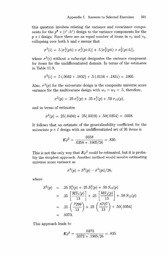
Appendix I. Answers to Selected Exercises 501

this question involves relating the variance and covariance compo­nents for the p. X (io : hO) design to the variance components for thep x i design. Since there are an equal number of items in VI and V2 ,

collapsing over both h and V means th at

o-2(i) = .5 [o-r(ph) + o-r(pi :h)] + .5 [o-~(ph) + o-~(pi :h )],

where o-2(i) without a subscript designates the variance componentfor items for th e undifferenti ated domain. In terms of the est imatesin Table 11.9,

cT 2(i ) = .5 (.0032 + .1832) + .5 (.0116 + .1831) = .1905.

Also, o-2(p) for the univariat e design is the composite universe scorevari ance for th e multivariat e design with W I = W2 = .5; therefore,

and in terms of estimates

cT2 (p) = .25(.0404) + .25(.0319) + .50(.0354) = .0358.

It follows that an est imate of the generalizability coefficient for theunivariate p x I design with an undifferenti at ed set of 26 items is

E , 2 = .0358 = .830.p .0358 + .1905/26

This is not the only way that E p2 could be estimated, but it is proba­bly the simplest approach. Anot her meth od would involve est imat inguniverse score variance as

where

S2(p) .25 S;(p) + .25 S;(p) + .50 SI2(p)

= .25 [M~~(P)] +.25 [M~~(P)] +.50SI 2(p)

(.7299) (.6727).25 ~ + .25 ~ + .50(.0354)

.0373.

This approach leads to

E , 2 = .0373 = .835.P .0373 + .1905/ 26

502 Appendix I. Answers to Selected Exercises

For the p. x W:hO) design, Table 11.10 reports that E/P = .801,which is smaller than the p x I estimates by about .03. Theory guar­antees that the multivariate result must be no larger than the univari­ate result. In this example, the difference is small because both of theestimated ph variance components for the multivariate p. x (i0 :hO)design are smalI.

11.13 Conceptually, the error variance in Equation 11.54 is given by Equa­tion 11.52 with n~ = 1. Using the Spearman-Brown formula has theeffect of halving every one of the variance and covariance componentsin Equation 11.52, which is precisely the same as using n~ = 2 in thatequation.

Chapter 12

12.1 This is a straightforward generalization of Equations 12.5 and 12.6recognizing that O'(Tv) = O'v(p) in the notation of this chapter.

12.3 Equation 12.18 states that

k

S,? = I)jSYXj 'j=1

In this case, k = n v , Y = Tv , and S~ = 0'2(J.lp). It follows that

which, with the addition of v subscripts, gives Equation 12.52.

12.5 We prove the result for VI ' The proof for V2 is entirely analogous. Forstandard scores, the variance of the regressed score estimates is R2(see Table 12.2). Therefore, it is sufficient to prove that

Using the expression for the ßs in Equation 12.26, this inequality is

(PI - P2P12r12) + (P2P12 - PIrl2) > 2

Pl 1 2 P2Pl2 1 2 - Pl-rl2 - r l2

or, equivalently,

pi - PlP2Pl2rl2 + p~pi2 - PlP2Pl2rl2 ~ pi(l - ri2)

P~pi2 - 2PlP2Pl2r 12 + Piri2 ~ 0

(P2Pl2 - Plrl2)2 ~ O.

The last inequality is necessarily true for all values of Pl, P2, PlZ , andr12·

App endix 1. Answers to Selected Exercises 503

12.7 The computations follow the steps illustrated in Section 12.2.2 for V I ,

with one primary except ion-the bl and b2 values are obtained usingEqu ation 12.30 instead of Equation 12.28. From anot her perspective,t he difference is that t he right side of the normal equations changes.For example, for the p. x r design with n~ = 8, the normal equationsfor V2 are

.5247b l + .4074b2

.4074bl + .561Ob2

.3193

.3689,

rather than those given by Equation 12.63 for V I .

12.9 Using the numerical results reported in Equations 12.46 to 12.49,

a 2 = ).3689 = .6074, SI = ).5769 = .7595,

PI = ) .6382 = .7989, P2 = ) .5902 = .7683, and P12 = .8663.

For th e p. x JO design, th ere is no correlat ed 8-typ e error, whichmeans that S12 = a1 2. It follows that

Using these numerical result s in Equ ation 12.30 gives b12 = .3162 andb22 = .4287. Using Equation 12.55,

a I2({1.p) = b12ar + b22a12 = (.3162)(.3682) + (.4287)(.3193) = .2533.

Finally, using Equation 12.61,

12.11 This is a "no-correlated-error" design in which th e error variances forthe design are of the 6. type. Frorn Table 9.3,

2 (A) _ .3444 + 1.2522 _ 66a l u - - .2 16

anda~ (6. ) = .3200 +1.5367 = .3094.

6

It follows that

S I = Jar (p) + ar (6.) = ).3682 + .2661 = .7964,

SI = Ja~ (p) + a~ (6. ) = ) .3689 + .3094 = .8236,

504 Appendix 1. Answers to Selected Exercises

2 .3682PI = (.7964)2 = .5804,

2 .3690P2 = (.8236)2 = .5438,

8 12 = 0"12(p) = .3193,

andT12 = 0"12(p) = .3193 = .4867.

8 182 .7964 X .8236

The estimated universe score variances and covariances and esti­mates of the means in the population and universe (Le., the sam­ple means) remain unchanged: O"r = .3682, O"~ = .3690, 0"12 = .3193,XI = 4.5167, and X 2 = 5.0833. Using these values in Equations 12.79to 12.81 gives the two-variable prediction

jlpc = .5118 - .1493 X p 1 + .1434 X p2 '

Using Equation 12.82,

R2 = - .1493(.3193 - .3682) + .1434(.3689 - .3193) = .1432.c .3682 + .3689 - 2(.3193)

For the single-variable regression, using Equation 12.85 (with ö,-typeerror variances replacing 8-type error variances) ,

2 _ 2 _ _ .2661 + .3094 _ 1462Ep - R - 1 .6343 + .6783 _ 2(.3193) - . ,

and the prediction equation is

12.12 Responses to this question make heavy use of the estimated universescore variance and covariance components determined in Section 9.1:

[

1.5714 1.4821 .5000]Ep = 1.4821 2.7857 .9464 .

.5000 .9463 1.8571

(a) We need to determine R2 given by Equation 12.19, based onthe fact that each of the three covariances between the compos­ite and an observed variable is given by Equation 12.70. Thesecovariances are

8YXl .25(1.5714) + .50(1.4821) + .25(.5000) = 1.2589

8y X2 = .25(1.4821) + .50(2.7857) + .25(.9464) = 2.0000

8yX3 .25(.5000) + .50(.9463) + .25(1.8571) = 1.0625.

Appendix 1. Answers to Selected Exercises 505

We have already determined in Section 9.1 that the compositeuniverse score variance is ab(p) = 1.5804. Therefore,

R2 _ 1.2589(.2446) + 2.0000(.4608) + 1.0625(.2433) _c - 1.5804 - .9416,

and the standard error of estimate is

adE) = )1.5804)1 - .9416 = .304.

The first person has observed scores of 4.50, 3.75, and 6.00,which give a predicted composite of 4.5219, and a 90% toleranceinterval of 4.52 ± 1.645(.304), or 4.52 ± .50.

(b) Using the :Ep values and the regression weights in the formulasfor a~(flp} and avv,(flp) in Equations 12.52 and 12.55, respec­tively, gives the following matrix of variances and covariancesfor the regressed score estimates of the universe scores,

[

1.3575 1.4499 .4988]:E{tp = 1.4499 2.5597 .9370 .

.4988 .9370 1.6687

That is, for example, ar(flp) = 1.3575 and a12(flp) = 1.4499.Dividing the elements of :E{tp by the elements of :Ep gives

[

.8639R = .9783

.9975

.9783

.9189

.9900

.9975 ]

.9900 .

.8985

That is, for example, Ri = .8639 and R 12 = .9783.

(c) nv for T scores is the same as nv for standard scores . There­fore,

nv = 1 _ (.8639 + .9189 + .8985)/ 3 = 1 _ .8938 = .934.(.8639 + .9783 + ...+ .8985}/9 .9570

This extraordinarily large value is attributable to the truly "syn­thetic" nature of these data!

References

ACT, Inc. (1976). User's guide: Adult APL Survey. Iowa City, Iowa: Au­thor.

ACT, Inc. (1997) . Content of the tests in the ACT Assessment. Iowa City,IA : Author.

Algina, J. (1989) . Elements of classical reliability theory and generalizabil­ity theory. Advances in Social Science Methodology, 1, 137-169.

AHal, L. (1988). Generalizability theory. In J . P. Keeves (Ed.) , Educationalresearch, methodology , and measurement (pp. 272-277) . New York:Pergamon.

AHal, L. (1990). Generalizability theory. In H. J . Walberg & G. D. Haertel(Eds.), The international encyclopedia of educational evaluation (pp.274-279) . Oxford, England: Pergamon.

American Educational Research Association, American Psychological As­sociation, & National Council on Measurement in Education (1999) .Standards for educational and psychological testing. Washington, DC:Author.

Arteaga, C., Jeyaratnam, S., & Graybill, F . A. (1982) . Confidence intervalsfor proportions of total variance in the two-way cross component ofvariance model. Communications in Statistics: Theory and Methods,11,1643-1658.

Bachman, L. F. , Lynch, B. K., & Mason, M. (1994). Investigating vari­ability in tasks and rater judgements in a performance test of foreignlanguage speaking. Language Testing , 12, 239-257.

508 References

Bell, J. F. (1985). Generalizability theory: The software problem. Journalof Educational Statistics, 10, 19-29.

Bell, J. F. (1986). Simultaneous confidence intervals for the linear functionsof expected mean squares used in generalizability theory. Journal ofEducational Statistics, 11, 197-205.

Betebenner, D. W. (1998, April). Improved confidence interval estimationfor variance components and error variances in generalizability the­ory. Paper presented at the Annual Meeting of the American Educa­tional Research Association, San Diego, CA.

Bock, R. D. (1975). Multivariate statistical methods in behavioral research.New York: McGraw-Hill.

Bock, R. D., Brennan, R. L., & Muraki, E. (2000). The information inmultiple ratings. Chicago: Scientific Software International.

Bollen, K. A. (1989). Structural equations with latent variables. New York:Wiley.

Boodoo , G. M. (1982). On describing an incidence sample. Journal of Ed­ucational Statistics, 7(4), 311-33l.

Boodoo, G. M. & O'Sullivan, P. (1982). Obtaining generalizability coeffi­cients for clinical evaluations. Evaluation and the Health Professions,5(3), 345-358.

Box, G. E. P. & Tiao, G. C. (1973). Bayesian inference in statistical anal­ysis. Reading, MA: Addison-Wesley.

Brennan, R. L. (1983). Elements of generalizability theory. Iowa City, IA:ACT, Inc.

Brennan, R. L. (1984). Estimating the dependability of the scores. In R.A. Berk (Ed.), A guide to criterion-referenced test construction (pp.292-334). Baltimore: Johns Hopkins University Press .

Brennan, R. L. (1992a). Elements of generalizability theory (rev. ed.) . IowaCity, IA: ACT, Inc.

Brennan, R. L. (1992b). Generalizability theory. Educational Measurement:Issues and Practice, 11(4), 27-34.

Brennan, R. L. (1994). Variance components in generalizability theory. InC. R. Reynolds (Ed.), Cognitive assessment: A multidisciplinary per­spective (pp. 175-207). New York: Plenum.

Brennan, R. L. (1995a). The conventional wisdom about group mean scores.Journal of Educational Measurement, 32, 385-396.

Brennan, R. L. (1995b). Standard setting from the perspective of gener­alizability theory. In Proceedings of the joint conference on standardsetting for large-scale assessments (Volume II) . Washington, DC: Na­tional Center for Education Statistics and National Assessment Gov­erning Board .

References 509

Brennan, R. 1. (1996a). Conditional standard errors of measurement ingeneralizability theory (Iowa Testing Programs Occasional Paper No.40). Iowa City, IA: Iowa Testing Programs, University of Iowa.

Brennan, R. L. (1996b) . Generalizability of performance assessments. InG. W. Phillips (Ed.). Technical issues in performance assessments.Washington, DC: National Center for Education Statistics.

Brennan, R. L. (1997). A perspective on the history of generalizabilitytheory. Educational Measurement: Issues and Practice, 16(4), 14-20 .

Brennan, R. L. (1998). Raw-score conditional standard errors of measure­ment in generalizability theory. Applied Psychological Measurement,22, 307-331.

Brennan, R. L. (2000a) . (Mis)conceptions about generalizability theory.Educational Measurement: Issues and Practice , 19(1),5-10.

Brennan, R. L. (2000b) Performance assessments from the perspective ofgeneralizability theory. Applied Psychological Measurement, 24, 339­353.

Brennan, R. L. (2001a). Manual for mGENOVA. Iowa City, IA: Iowa Test­ing Programs, University of Iowa.

Brennan, R. L. (2001b). Manualfor urGENOVA. Iowa City, IA: Iowa Test­ing Programs, University of Iowa.

Brennan, R. L. (in press) . An essay on the history and future of reliabilityfrom the perspective of replications. Journal of Educational Measure­ment.

Brennan, R. L. & Johnson, E. G. (1995). Generalizability of performanceassessments. Educational Measurement: Issues and Practice, 14 (4),9-12.

Brennan, R. L. & Kane, M. T. (1977a) . An index of dependability formastery tests. Journal of Educational Measurement, 14, 277-289.

Brennan, R. L. & Kane , M. T. (1977b). Signal/noise ratios for domain­referenced tests. Psychometrika, 42, 609-625.

Brennan, R. L. & Kane , M. T . (1979). Generalizability theory: A review.In R. E. Traub (Ed .), New directions for testing and measurement:Methodological developments (NoA) (pp. 33-51) . San Francisco:Jossey-Bass.

Brennan, R. L. & Lockwood, R. E. (1980). A comparison of the Nedelskyand Angoff cutting score procedures using generalizability theory. Ap­plied Psychological Measurement, 4, 219-240.

Brennan, R. L., Gao, X., & Colton, D. A. (1995). Generalizabilityanalysesof Work Keys listening and writing tests. Educational and Psycholog­ical Measurement, 55, 157-176.

510 References

Brennan, R. L., Harris, D. J., & Hanson, B. A. (1987). The bootstrap andother procedures for examining the variability of estimated variancecomponents in testing contexts (American College Testing ResearchReport No. 87-7). Iowa City, IA: ACT, Inc.

Burdick, R. K. & Graybill , F. A. (1992). Confidence intervals on variancecomponents. New York: Dekker.

Burt, C. (1936). The analysis of examination marks. In P. Hartog & E. C.Rhodes (Eds.), The marks of examiners. London: Macmillan .

ButterfieId, P. S., Mazzaferri, E. L., & Sachs, L. A. (1987). Nurses as evalua­tors of the humanistic behavior of internal medicine residents . Journalof Medical Education, 62, 842-849.

Cardinet, J. & Tourneur, Y. (1985). Assurer La measure. New York: PeterLang.

Cardinet, J., Tourneur, Y., & Allal, L. (1976). The symmetry of generaliz­ability theory: Applications to educational measurement. Journal ofEducational Measurement, 13, 119-135.

Cardinet, J., Tourneur, Y., & Allal, L. (1981). Extension of generalizabilitytheory and its applications in educational measurement . Journal ofEducational Measurement, 18, 183-204.

Chambers, D. W. & Loos, L. (1997). Analyzing the sources of unreliabilityin fixed prosthodontics mock board examinations. Journal of DentalEducation, 61, 346-353.

Clauser, B. E ., Harik, P., & Clyman, S. G . (2000) . The generalizabil­ity of scores for a performance assessment scored with a computer­automated scoring system . Journal of Educational Measurement, 37,245-261.

Cochran, W. G. (1977). Sampling techniques (3rd ed.). New York: Wiley.

Collins, J. D. (1970). Jackknifing generalizability. Unpublished doctoral dis­sertation, University of Colorado, Boulder.

Cornfield, J. & Tukey, J. W. (1956). Average values of mean squares infactorials. Annals of Mathematical Statistics, 27, 907-949.

Crick, J. E. & Brennan, R. L. (1983). Manual for GENOVA: A general­ized analysis of variance system (American College Testing TechnicalBulletin No. 43). Iowa City, IA: ACT, Inc.

Cracker, L., & Algina, J. (1986). Introduction to classical and modern testtheory. New York: Holt .

Cranbach, L. J. (1951). Coefficient alpha and the internal structure oftests.Psychometrika, 16, 292-334.

Cranbach, L. J . (1976). On the design of educational measures . In D. N. M.de Gruijter & L. J. T . van der Kamp (Eds.), Advances in psychologicaland educational measurement (pp. 199-208). New York: Wiley.

References 511

Cronbach , L. J . (1991) . Methodological studies-A personal retrospective.In R. E. Snow & D. E. Wiley (Eds .) , Improving in quiry in social sei­ence: A volume in honor of Lee J. Cronbach (pp, 385- 400). Hillsdale,NJ: Erlbaum.

Cronbach, L. J . & Gleser , G. C. (1964). The signal/nolse rat io in the com­par ison of reliabili ty coefficients. Educational and Psychological Mea­surement, 24, 467- 480.

Cronbach, L. J ., Gleser , G. C., Nanda, H., & Raj aratnam , N. (1972). Thedependabilit y of behavioral measureme nts: Theory of generalizabilit y[or scores and profiles. New York: Wiley.

Cronbach, L.J. , Linn , R. L., Brenn an , R. L., & Haertel, E. (1997). General­izability analysi s for performance assessments of st udent achievementor school effect iveness . Educational and Psychological Measurement,57, 373-399.

Cronbach , L. J ., Rajaratnam , N., & Gleser , G. C. (1963) . Theory of gen­era lizability: A liberalization of reliability theory. Brit ish Journal ofStatistical Psychology, 16, 137-163.

Cronbach, L. J ., Schönemann, P., & McKie, T. D. (1965). Alpha coefficientsfor st ra t ified-para llel tes ts . Edu cational and Psychological Measure­ment, 25, 291-312.

Crooks, T . J . & Kane, M. T. (1981). The generalizability of student ratingsof inst ru ctors: Item specificity and section effects . Research in HigherEducation, 15, 305-313.

Crowley, S. L. , Thomp son , B. , & Worchel, F. (1994). T he Chil dren 's De­pression Inventory: A comparison of generalizability and classicaltest t heory analyses. Educational and Psychological Measurement, 54,705-713 .

Demorest, M. E. & Bernstein , L. E. (1993) . Applications of genera lizabilitytheory to measurement of individual differences in speech perception .Journ al of the Academ y of Rehabilitative Audiology, 26, 39-50.

Dunbar , S. B. , Kor etz , D. M., & Hoover , H. D. (1991). Quality cont rol inthe development and use of performance assessments . Applied Mea­sureme nt in Edu cation, 4, 289- 303.

Dunnet te, M. D. & Hoggatt , A. C. (1957). Deriving a composite score fromsevera l measures of th e same attribute . Edu cational and PsychologicalMeasureme nt, 17, 423- 434.

Eb el, R. L. (1951) . Est imation of t he reliability of ratings. Psychometrika ,16, 407-424.

Efron , B. (1982). The ja ckknife, the bootstrap, and other resampling plans .Philadelphia: SIAM.

512 References

Efron, B. & Tibshirani, R. (1986). Bootstrap methods for standard errors,confidence intervals, and other measures of statistical accuracy. Sta­tistical Science, 1, 54-77 .

Feldt, L. S. (1965). The approximate sampling distribution of Kuder­Richardson reliability coefficient twenty. Psychometrika, 30,357-370.

Feldt, L. S. & Brennan, R. L. (1989). Reliability. In R. L. Linn (Ed .), Edu­cational measurement (3rd ed.) (pp. 105-146). New York: AmericanCouncil on Education and Macmillan.

Feldt, L. S. & Qualls, A. L. (1996). Estimation of measurement error vari­ance at specific score levels. Journal 0/Educational Measurement, 33,141-156.

Feldt, L. S., Forsyth, R. A., Ansley, T . N., & Alnot, S. D. (1994). Iowatests 0/educational development: Interpretative guide [or teachers andcounselors (Levels 15-18). Chicago: Riverside.

Finn, A. & Kayande, U. (1997). Reliability assessment and optimizationof marketing measurement. Journal 0/ Marketing Research , 34, May,262-275.

Fisher, R. A. (1925). Statistical methods jor research workers. London:Oliver & Bond.

Fuller , W. A. (1987). Measurement error models. New York: Wiley.

Gao, X. & Brennan, R. L. (2001). Variability of estimated variance com­ponents and related statistics in a performance assessment . AppliedMeasurement in Education, 14, 191-203 .

Gillmore, G. M., Kane, M. T., & Naccarato, R. W. (1978). The generaliz­ability of student ratings of instruction: Estimation of the teacher andcourse components. Journal 0/ Educational Measurement, 15, 1-14.

Gleser, G. C., Cronbach, L. J ., & Rajaratnam, N. (1965). Generalizabilityof scores influenced by multiple sources of variance. Psychometrika,30, 395-418.

Graybill , F. A. (1976). Theory and application 0/ the linear model. NorthScituate, MA: Duxbury.

Graybill , F. A. & Wang, C. M. (1980). Confidence intervals on nonnegativelinear combinations of variances. Journal 0/ the American StatisticalAssociation, 75, 869-873.

Gulliksen, H. (1950). Theory 0/ mental tests. New York: Wiley. [Reprintedby Lawrence Erlbaum Associates, Hillsdale, NJ, 1987.]

Hartley, H. O. (1967). Expectations, variances , and covariances of ANOVAmean squares by 'synthesis.' Biometries, 23, 105-114, and Corri­genda, 853.

References 513

Hartley, H. 0. , Raa , J. N. K. , & LaMotte, L. R (1978). A simple 'synthesis'­based method of varian ce component estimat ion. Biometrics, 34,233-242 .

Hartman , B. W. , Fuqua, D. R , & Jenkins, S. J . (1988). Multivariat e gener­alizability analysis of three measures of career indecision. Educationaland Psychological Measurement, 48, 61-68.

Hatch, J . P., Prihoda, T . J ., & Moore, P. J . (1992). The applicat ion ofgeneralizability theory to surface electromyographic measurementsduring psychophysiological st ress testing: How many measurementsare needed? Biofeedback and Self Regulation, 17, 17-39.

Henderson, C. R (1953). Estimation of variance and covariance compo­nents. Biom etrics, g, 227-252.

Hoover , H. D. & Bray, G. B. (1995, April) . The research and developm entphrase: Can a performance assessment be cost-effective? Paper pre­sented at the Annual Meetin g of the American Educational ResearchAssociation, San Francisco, CA.

Hoover , H. D., Hieronymus, A. N., Frisbie, D. A., & Dunbar, S. B. (1994).Iowa writin g assessment (Levels 9-14) . Chicago: Riverside.

Hoover , H. D., Hieronymus, A. N., Frisbie, D. A., Dunbar , S. B., Oberley,K. A., Cantor, N. K., Bray, G. B., Lewis, J. C. , & Qualls, A. L.(1993). Iowa tests of basic skills: Interpretat ive guide for teachersand counselo rs (Levels 9-14). Chicago: Riverside.

Hoyt , C. J. (1941). Test reliability est imated by analysis of variance. Psy­chome trika, 6, 153-1 60.

Huynh , H. (1977, April ). Estimation of the KR20 reliability coefficient whendata are incomplete. Paper presented at the Annual Meeting of theAmerican Edu cational Research Association, New York.

Jarjoura, D. (1983). Best linear prediction of composite universe scores.Psychometrika, 48, 525-539.

Jarjoura, D. (1986). An est imator of examinee-Ievel measurement errorvariance th at considers test form difficulty adjustments . Applied Psy­chological Measurement, 10, 175-186.

Jarjoura, D. & Brennan , R L. (1981, January) . Three variance componentsmodels for some measurement procedures in which un equal num bersof items fall into discrete categories (American College Testing Tech­nical Bulletin No. 37). Iowa City, Ia: ACT , Inc.

Jarjoura, D. & Brennan, R L. (1982). A variance components model formeasurement procedures associated with a table of specificat ions. Ap­plied Psychological Measurement, 6, 161-171.

Jarjoura, D. & Brennan , R. L. (1983). Multivariate generalizability mod­els for tests developed according to a t able of specifications. In L. J.

514 References

Fyans (Ed.), New directions [or testing and measurement: Generaliz­ability theory (No.18) (pp. 83-101). San Francisco: Jossey-Bass.

Joe, G. W. & Woodward, J. A. (1976). Some developments in multivariategeneralizability. Psychometrika, 41 (2), 205-217.

Johnson, S. & Bell, J . F. (1985). Evaluating and predicting survey efficiencyusing generalizability theory. Journal of Educational Measurement,22, 107-119.

Jöreskog, K. G. & Sörbom, D. (1979). Advances in factor analysis andstructural equation models. Cambridge, MA: Abt.

Jöreskog, K. G. & Sörbom, D. (1993). LISREL 8: User's reference guide.Chicago: Scientific Software International.

Kane, M. T . (1982) . A sampling model for validity. Applied PsychologicalMeasurement, 6, 125-160.

Kane, M. T. (1996). The precision of measurements. Applied Measurementin Education, 9, 355-379.

Kane, M. T . & Brennan, R. L. (1977). The generalizability of dass means,Review of Educational Research, 47, 267-292.

Kane, M. T., Crooks, T. J., & Cohen, A. (1999). Validating measures ofperformance. Educational Measurement: Issues and Practice, 18 (2),5-17.

Kane, M. T ., Gillmore, G. M., & Crooks, T. J. (1976). Student evaluationsof teaching: The generalizability of dass means. Journal of Educa­tional Measurement, 13, 171-183.

Kelley, T. L. (1947). Fundamentals of statistics. Cambridge, MA: HarvardUniversity Press.

Kendall, M. & Stuart, A. (1977). The advanced theory of statistics (4th ed.,Vol. 1). New York: Macmillan.

Khuri, A. 1. (1981). Simultaneous confidence intervals for functions ofvari­ance components in random models . Journal of the American Statis­tical Association, 76, 878-885.

Klipstein-Grobusch, K., Georg, T., & Boeing, H. (1997). Interviewer vari­ability in anthropometrie measurements and estimates of body com­position. International Journal of Epidemiology, 26(Suppl. 1), 174­180.

Knight, R. G., Ross, R. A., Collins, J. 1., & Parmenter, S. A. (1985) . Somenorms, reliability and preliminary validity data for an S-R inventoryof anger: The Subjective Anger Scale (SAS). Personality and Indi­vidual Differences, 6, 331-339.

Koch, G. G. (1968) . Some further remarks concerning "A general approachto the estimation of variance components." Technometrics, 10, 551­558.

References 515

Kolen , M. J . (1985). Standard errors of Tucker equating. Applied Psycho­logical Measurement, 9, 209-223.

Kolen , M. J . & Brennan, R. L. (1995). Test equating methods and practices.New York: Springer-Verlag.

Kolen, M. J . & Harris , D. J. (1987, April) . A multivariate test theory modelbased on item response theory and generalizability theory. Paper pre­sented at the Annual Meeting of the American Educational ResearchAssociation, Washington, DC.

Kolen , M. J. , Hanson, B. A., & Brennan, R. L. (1992). Conditional stan­dard errors of measurement for scale scores. Journal of EducationalMeasureme nt, 29, 285-307 .

Kreiter, C. D., Brennan, R. L., & Lee, W. (1998). A generalizability studyof a new standardized rating form used to evaluate students' clinicalclerkship performance. Academic Medicine , 73, 1294-1298.

Kuder , G. F. & Richar dson, M. W. (1937). The theory of estimation oftestreliability. Psychometrika , 2, 151-160.

Lane , S., Liu, M., Ankenmann, R. D., & Stone, C. A. (1996). Generalizabil­ity and validity of a mathematics performance assessment. Journalof Educational Measurement , 33, 71-92.

Lee, G., Brennan, R. L., & Frisbie , D. A. (2001). Incorporating the testletconcept in test score analys es. Educational Measurement: Issues andPractice, 19 (4), 5-9.

Lee, W., Brennan, R. L., & Kolen, M. J . (2000). Estimators of conditionalscale-score standard errors of measurement: A simulation study. Jour­nal of Educational Measurement, 37, 1-20 .

Leucht, R . M . & Smith, P. L. (1989, April) . The effects of bootstrappingstrategies on the estimation of variance components. Paper presentedat the Annual Meeting of the American Educational Research Asso­ciation, San Francisco , CA.

Lindquist , E. F . (1953). Design and analysis of experiments in psychologyand education. Boston: Houghton Mifflin.

Linn, R. L. & Burton, E. (1994). Performance-based assessment: Implica­tions of task specificity. Educational Measurement: Issues and Prac­tice, 13(1) ,5-8, 15.

Linn, R. L. & Werts, C. E. (1979). Covariance structures and their anal­ysis. In R. E. Traub (Ed .), New directions for testing and measure­ment : Methodological developments (No. 4) (pp . 53-73) . San Fran­cisco: Jossey-B ass.

Llabre, M. M., Ironson, G. H., Spitzer, S. B., Gellman, M. D., Weidler , D. J .,& Schneiderman, N. (1988). How many blood pressure measurements

516 References

are enough?: An application of generalizability theory to the studyof blood pressure reliability. Psy chophysiology, 25, 97-106

Loevinger, J. (1965). Person and population as psychometrie concepts. Psy­chological Review, 72, 143-155.

Longford, N. T. (1995). Models [or uncertainty in educational testing. NewYork: Springer-Verlag.

Lord , F. M. (1955). Estimating test reliability. Educational and Psycholog­ical Measurement, 15, 325-336.

Lord , F. M. (1956) . The measurement of growth. Edu cational and Psycho­logical Measurement, 16,421-437.

Lord , F. M. (1957). Do tests of the same length have the same standarderror of measurement? Educat ional and Psy chological Measurement ,17, 510-521.

Lord , F. M. (1958). Further problems in the measurement of growth. Ed­ucational and Psychological Measurement , 18, 437-451.

Lord, F. M. & Novick, M. R. (1968). Statisti cal theories 0/ mental testscores. Reading, MA: Addison-Wesley.

Marcoulides, G. A. (1998). Applied generalizability t heory models. In G. A.Marcoulides (Ed .), Modern methods [or business research. Mahwah ,NJ : Erlbaum.

Marcoulides, G. A. & Goldstein, Z. (1990). The optimization of generaliz­ability studies with resource const raints. Educational and Psycholog­ical Measurement, 50, 761-768.

Marcoulides, G. A. & Goldstein, Z. (1992). The optimization of multivari­ate generalizability studies with budget constraints. Educational andPsychological Measurement, 52, 301-308.

MathSoft , Inc. (1997). S-Plus 4.5 standard edition. Cambridge, MA: Au­t hor.

McNemar , Q. (1958). On growth measurement. Educational and Psycho­logical Measurement , 18, 47-55.

Miller , T . B. & Kane, M. T. (2001, April) . The precision 0/ change scoresunder absolute and relative interpretations. Paper presented at theAnnual Meeting of the National Council on Measurement in Educa­ti on , Seattle, WA.

Norcini , J . J ., Lipner, R. S., Langdon, L. 0 ., & Strecker , C. A. (1987). Acomparison of three variations on a standard- setting method. Journal0/ Educational Measurement , 24, 56-64.

Nußbaum, A. (1984). Multivariat e generalizability t heory in educationa lmeasurement: An empirical study. Appli ed Psychological Measure­ment, 8(2) , 219-230.

References 517

Oppliger , R. A. & Spr ay, J. A. (1987). Skinfold measurement vari ability inbo dy density prediction . Research Quarterly [or Ezercise and Sport ,58, 178-1 83.

Othman , A. R. (1995) . Examining task sampling variability in science per­formance assessments. Unpublished doctoral dissert ation , Universityof California , Santa Barbara.

Quenouille, M. (1949). App roxim ation tests of corre lation in time series.Journal of the Royal Sta tistical Society B, 11, 18-24.

Raj ara tnam , N., Cronbach, L. J ., & Gleser , G. C. (1965) . Generalizabilityof st ra t ified-parallel test s. Psychometrika, 30, 39-56 .

Rentz , J. O. (1987). Generalizabili ty theory: A comprehensive method forassessing and imp roving the dependability of marketing measures.Journal of Marketing Research, 24 (February) , 19-28.

Ruiz-Primo, M. A., Baxter , G. P. , & Shavelson, R. J. (1993). On the stabil­ity of performance assessments, Journal of Edu cational Measurement,30, 41-53.

SAS Institute, Inc. (1996). The SAS system [or Wind ows release 6.12. Cary,NC : Author.

Sattert hwaite , F. E. (1941) . Synt hesis of variance. Psychometrika, 6, 309­316.

Sattert hwaite, F . E . (1946). An approximate distribution of est imates ofvariance compo nents. Biometries Bulletin, 2, 110-114.

Scheffe, H. (1959). The analysis of variance . New York: Wiley.

Searle, S. R. (1971). Linear models. New York: Wiley.

Searle, S. R. (1974) . Prediction , mixed mod els, and variance components.In F . P roschan & R. J. Sterfling (Eds.) , Reliability and biom etry .Philadelphia: SIAM.

Searl e, S. R., Casella , G. , & McCulloch, C. E. (1992). Variance components.New York : Wiley.

Shao , J. & TU, D. (1995) . The jackknife and the bootstrap. New York:Springer-Verlag.

Shavelson , R. J. & Demp sey-Atwood, N. (1976). Generalizability of mea­sures of teaching behavior . Review of Educational Research, 46, 553­611.

Shavelson , R. J . & Webb, N. M. (1981). Generalizability theory: 1973­1980. Brit ish Journal of Math ematical and Statistical Psychology, 34,133-1 66.

Shavelson , R. J. & Webb, N. M. (1991). Generalizability theory: A primer.Newb ury Park, CA: Sage .

518 References

Shavelson, R. J. & Webb, N. M. (1992). Generalizability theory. In M. C.Alkin (Ed.), Encyclopedia of educational research (Vol. 2) (pp. 538­543) . New York: Macmillan.

Shavelson, R. J., Baxter, G. P., & Gao, X. (1993). Sampling variability ofperformance assessments. Journal of Educational Measurement, 30,215-232.

Shavelson, R. J ., Webb , N. M., & Rowley, G. L. (1989). Generalizabilitytheory. American Psychologist, 6, 922-932 .

Sireci, S. G., Thissen, D., & Wainer, H. (1991). On the reliability of testlet­based tests. Journal of Educational Measurement, 28, 237-247.

Sirotnik, K. & Wellington, R. (1977) . Incidence sampling: An integratedtheory for "matrix sampling." Journal of Educational Measurement,14, 343-399.

Smith, P. L. (1978). Sampling errors of variance components in small sam­ple generalizability studies. Journal of Educational Statistics, 3, 319­346.

Smith, P. L. (1982). A confidence interval approach for variance componentestimates in the context of generalizability theory. Educational andPsychological Measurement, 42,459-466.

Snedecor, G. W. & Cochran, W. G. (1980). Statistical methods. Ames, IA:Iowa University Press.

SPSS, Ine. (1997). SPSS for Windows releose 8.0.0. Chicago: Author.

Strube, M. J. (2000). Reliability and generalizability theory. In L. G. Grimm& P. R. Yarnold (Eds.), Reading and understanding more multivari­ate statistics (pp, 23-66) . Washington, DC: American PsychologicalAssociation.

Thompson, B. & Melancon, J . G. (1987). Measurement eharacteristics ofthe Group Embedded Figures Test . Educational and PsychologicalMeasurement, 47, 765-772 .

Ting, N., Burdick, R. K., Graybill, F . A., Jeyaratnam, S., & Lu, T. C.(1990) . Confidence intervals on linear combinations of variance com­ponents that are unrestrieted in sign. Journal of Statistical Compu­tational Simulation, 35, 135-143.

Tobar, D. A., Stegner, A. J ., & Kane, M. T. (1999). The use of generaliz­ability theory in examining the dependability of score on the Profileof Mood States. Measurement in Physical Education and EiereiseScience, 3, 141-156.

Tukey, J. W. (1958). Bias and confidence in not quite large samples. Annalsof Mathematical Statistics, 29, 614.

Ulrich, D. A., Riggen, K. J ., Ozmun, J. C., Screws, D. P., & Cleland, F .E. (1989) . Assessing movement control in children with mental retar-

References 519

dati on: A generalizability analysis of observers. American Journal ofMental Retardation, 94, 170-176 .

Wainer, H. (1993). Measurement problems. Journal of Edu cational Mea­surement, 30, 1-2 l.

Wainer , H. & Kiely, G. L. (1987). It em clusters and compute rized adaptivetesting: A case for testlets. Journal of Educational Measurement, 24,185-20l.

Wainer , H. & Lewis, C. (1990). Toward a psychometr ics for testlets. Journalof Edu cational Measurement, 27, 1-14 .

Wang , M. D. & Stanley, J. C. (1970). Differential weighting: A review ofmethods and empirical studies. Review of Edu cational Research, 40,663-705 .

Webb , N. M. & Shavelson, R. J . (1981). Multivariat e generalizability ofGeneral Educational Development ratings. Journal of Educationa lMeasurem ent , 18, 13-22.

Webb , N. M., Schlackman , J ., & Sugrue, B. (2000). The dependability andinterchangeability of assessment methods in science. Applied Mea­sureme nt in Edu cation 13, 277- 30l.

Webb, N. M., Shavelson, R. J., & Madd ahian , E. (1983). Mult ivariate gen­eralizability theory. In L. J. Fyans (Ed.) , New direction s in testingand measurement: Generalizability theory (No. 18) (pp. 67- 82). SanFrancisco: Jossey-Bass.

Wiley, E. W. (2000). Bootstrap strategies for variance component estima­tion: Theoretical and empirical results. Unpublished doctoral disser­t ation, Stanford .

Wilks, S. S. (1938) . Weighting systems for linear functions of corre latedvari ables when there is no dependent variable. Psychom etrika, 3, 23­40.

Winer, B. J . (1971). St atistical prin ciples in experimental design. New York :McGraw-Hill.

Wohlgemuth, W. K., Edinger , J . D., Fins, A. 1., & Sullivan, R. J. (1999).How many nights are enough? The short-term stability of sleep pa­rameters in elderly insomniacs. Psychophysiology, 36, 233-244.

Author Index

A

Algina, J ., 4, 507, 510Allal , L., 4, 507, 510Alnot, S. D. , 512Ankenmann, R. D., 515Ansley, T . N., 512Arteaga , C., 200, 207, 208, 507

B

Bachman , L. F ., 17, 507Baxter , G. P., 517, 518Bell, J . F., 18,210,243, 508,514Bernstein, L. E. , 18, 511Bet ebenner, D. W., 179, 192, 209,

508Bock, R. D., 176, 287, 508Boeing, H., 514Bollen , K. A., 174, 508Bood oo, G. M., 18, 209, 508Box, G. E. P., 85, 508Bray, G . B., 117, 513Brennan, R. L., ix, 2-4, 17, 20, 22,

24, 30, 34, 35, 47, 48, 50,68, 86, 88, 97, 117, 118,129, 130, 135, 151, 156-1 58,160,164,165,179 ,1 80,1 83,

186, 187, 191, 210, 215, 225,230,241 ,245,267,268,275,280,302,308,312,317,328,331,339,341,344,418,419,425,445 ,453,471 ,473,508­515

Burdick, R. K. , 179, 180, 190-193,198, 200, 210, 510, 518

Burt , C., 3, 510Burton, E., 17, 515Butterfieid, P. S., 18, 510

C

Cantor, N. K. , 513Cardinet, J ., 4, 108, 156, 510Casella, G., 517Chambers , D. W., 18, 510Clauser , B. E. , 18, 510Cleland , F. E., 519Clyman, S. G., 510Cochran, W. G., 142, 174, 510, 518Cohen, A., 117, 514Collins, J . D., 196, 510Collins , J . 1., 514Colton, D. A., 509Cornfield, J ., 77,88,155,172,175,

183, 510

522 Author Index

Crick, J . E ., 453, 510Crocker, L., 4, 510Cronbach, L. J ., vii, viii, 3, 4,19,22­

24, 29, 34, 35, 47, 62, 79,84, 88, 89, 102, 117, 135,147,149,165,168-170,179,183,185,230,243,263,267­269,274,275,285,287,295,301,366,458,510-512,517

Cronbach, LoJ., 511Crooks, T . J ., 17, 117, 511, 514Crowley, S. L., 17, 511

D

Demorest, M. n., 18, 511Dempsey-Atwood, N., 17,517Dunbar, S. B., 135, 511, 513Dunnette, M. D., 313, 511

E

Ebel, R. L., 3, 511Edinger, J. n., 519Efron, B., 185, 189, 196, 511, 512

F

FeIdt, L. S., 2, 4, 37, 160, 162, 198,199,205,207,208,212,252,282,344,373,418,419,425,512

Finn, A., 17, 512Fins, A. 1., 519Fisher, R. A., 2, 512Forsyth, R. s., 512Frisbie, n. A., 513, 515Fuller, W . A., 174,512Fuqua, D. R., 513

G

Gao , X., 179, 509, 512, 518Gellman, Mo D., 516Georg, T ., 514Gillmore, G. M., 92, 138, 512, 514Gleser, G o C o, vii , 3, 47, 268, 511,

512, 517Goldstein, Z., 313, 516Graybill, Fo s.. 179, 180, 190-193,

195,198,200,210,507,510,512, 518

Gulliksen, H., 117, 135, 512

H

Haertel, E ., 511Hanson, B. s .;510, 515Harik, P., 510Harris, D. J ., 176,510,515Hartley, H. 0 ., 241, 243, 512, 513Hartman, B. Wo, 17, 513Hatch, J . P., 18, 513Henderson, C. R., 217, 222, 242, 254,

471,513Hieronymus, A. N., 513Hoggatt , A. C., 313, 511Hoover , H. D., 37, 50,117,284,367,

511,513Hoyt, C . J ., 3, 513Huynh, H., 226, 513

I

Ironson, G. H., 516

J

JaDoura,D. , 170,215,225,268,302,308, 312, 425, 513, 514

Jenkins, S. J ., 513Jeyaratnam, S., 507, 518Joe, G. W ., 313, 514Johnson, E, G. , 117, 509Johnson, So , 18, 514Jöreskog, K. G., 174, 514

K

Kane, M. T ., 4, 17, 35, 47, 48, 106,117,130-132,134,158,509,511, 512, 514, 516, 518

Kayande, U., 17,512Kelley, T . L., 169, 514Kendall, M., 293, 514Khuri, A. 1., 210, 514Kiely, G. L., 262, 519Klipstein-Grobusch, K. , 18, 514Knight, R. Go, 17, 514Koch, GoG., 242, 514Kolen, Mo J ., 166, 176,293,294,331,

515Koretz, n. M., 511

Kreiter, C. D., 257-259, 515Kuder, G. F., 149, 515

L

LaMotte, L. R., 513Lane, S., 38, 163, 515Langdon, L. 0 ., 516Lee, G., 262, 265, 515Lee, W., 166, 515Leucht , R. M., 186, 515Lewis , C., 262, 519Lewis, J. C., 513Lindquist , E. F., 3, 515Linn , R. L., 17, 174, 511, 515Lipner, R. S., 516Liu , M., 515Llabre, M. M., 38, 39, 138, 516Lockwood , R. E. , 50, 509Loevinger, J. , 172,516Longford , N. T ., 166, 516Loos, L., 18, 510Lord , F . M., 33, 132, 151, 160, 161,

172, 175,418,516Lu, T . C., 518Lynch, B. K ., 507

M

Maddahian, E. , 519Marcoulid es, G . A., 17, 313, 516Mason , M., 507Mazzaferri , E. 1. , 510McCulloch, C. E. , 517McKie, T . D., 511McNemar , Q., 418, 516Melancon, J . G., 17,518Miller , T . B., 516Moore , P. J. , 513Muraki , E., 508

N

Naccarato, R. W., 512Nanda, H., vii, 511Norcini , J. J ., 17,516Novick, M. R. , 33,132,151 , 172,175 ,

516Nußbaum, A., 279, 334, 337, 338,

516

Author Index 523

oO'Sullivan, P., 18, 508Oberley, K. A., 513Oppliger, R. A., 18,517Othman, A. R., 186, 517Ozmun, J. C., 519

p

Parmenter, S. A., 514Prihoda , T . J. , 513

Q

Qualls, A. L., 160, .512, 513Quenouille, M., 182, 517

R

Rajaratnam, N., vii, 3, 225, 268, 269,343,428,511 ,512,517

Rao, J . N. K., 513Rentz, J . 0 ., 4, 517Richardson , M. W. , 149, 515Riggen , K. J ., 519Ross , R. A., 514Rowley, G. L., 518Ruiz-Primo, M. A., 120,517

sSachs , L. A., 510Satterthwaite, F . E., 190-192, 195­

197,203, 205,208,209 ,445,472, 517

Scheffe, H., 87, 273, 517Schlackman , J ., 519Schneiderman, N., 516Schönemann, P., 511Screws, D. P., 519Searle, S. R., 77, 87, 166, 170, 179,

181,190,215,219,222,226,228,240,241 ,243,293, 360,426,439,451 ,517

Shao, J ., 182, 185, 196,209,517Shavelson, R. J ., 4,17,18, 117,118,

120,177,267,517-519Sireci, S. G., 262, 518Sirotnik, K ., 175, 209, 242, 518Smith, P. L., 179, 186, 515, 518Snedecor , G. W ., 174, 518

524 Author Index

Spitzer, S. B., 516Spray, J . A., 18,517Stanley, J . C., 307, 519Stegner, A. J ., 518Stone, C. A., 515Strecker, C. A., 516Strube, M. J ., 4, 518Stuart, A., 293, 514Sugrue, B., 519Sullivan, R. J ., 519Sörbom, D., 174,514

T

Thissen, D., 518Thompson, B., 17,511 ,518Tiao, G. C., 85, 508Tibshirani, R. , 185, 189, 196, 512Ting,N., 191, 192,195-197, 203, 205,

208,209,211 ,472,518Tobar , D. A., 18, 518Tourneur , Y., 4, 510Tu, D., 182, 185, 196, 209, 517Tukey, J . W., 77, 88,155, 172, 175,

182, 183, 510, 518

vUlrich, D. A., 18, 519

wWainer , H., 120, 262, 518, 519Wang , C. M., 195, 512Wang , M. D., 307, 519Webb, N. M., 4, 18, 120, 267, 298,

517-519Weidler , D. J ., 516Wellington, R. , 175, 209, 242, 518Werts, C. E. , 174, 515Wiley, E. W., 179, 186, 187, 190,

196, 197, 201, 209, 519Wilks , S. S., 313, 519Winer , B. J ., 212, 519Wohlgemuth, W. K., 18, 519Woodward, J . A., 313, 514Worchel, F ., 511

Subject Index

A

A , 80- 81Absolute error ß , 11, 32,42, 46, 100,

144Absolute erro r variance and SEM

compared with rela t ive error vari­ance, 13, 33-34, 43- 44, 103­104

conditio nal, 229, 232, 234, 236,260

definition , 101, 156exercises , 20, 50, 137, 139, 176,

266for mixed models, 14, 122-125for random models , 11-12, 16,

32, 46, 100-101rules ,

mixed model, 122random model, 101, 109

for total score metric, 49unbalanced designs, 228- 229, 231­

232, 234Venn diagrams 106-107, 123­

124"Achilles heel" argum ent , 210Algorithms for

est imating varian ce components,80-82,84,439, 455, 458

exercise, 92

expressing score effects, 66-67,70,96

Analogous

MP term s, 351, 373- 376

MS te rms , 253, 368, 373-376expected values, 221-222, 224,

225

SS term s , 220, 226, 253, 450­451

T terms, 218, 223-224, 253, 450-451

and C t erms , 358

and C P terms, 366

exercise, 247

exp ected values, 219- 223, 225

in mGENOVA, 388

and missing data, 363

and TP te rms , 349, 351, 362

TP term s, 348, 349- 353, 362,366

exercises, 388-389expected valu es, 350-351

526 Subject Index

Analogous-ANOVA procedure, 215,217-220,241-242,244,246,471

Analysis of means, 242-243Analysis of variance (ANOVA), vii,

2-4, 25, 58, 67-74Angoff procedure, 50ANOVA procedure, 8,25,27,29,53,

77,90,216Arteaga et al. confidence interval, 200,

208

B

Balanced designs . See Designs, bal­anced

Bayesian, 85, 169Best linear predictors (BLPs), 170,

171,425-426Bias(ed)

in bootstrap procedures, 186­190,212

caused be hidden facets, 325­326

D study estimated variance com­ponents, 241

EMS procedure, negative esti­mates 85

estimate of universe score, 169estimate of variance, 323, 403­

404, 406, 440setting negative estimates to zero,

85, 297(X - >.)2 as an estimate of

(p, - >.?, 48Bonferroni inequality, 210Bootstrap procedure, 179, 180, 208

bias , 186-190, 212confidence intervals, 196estimated standard errors, 185-

190Box-bar plots, 116, 126, 250,482

exercise, 137BQUE, 77, 216

cClassical test theory

assumptions for difference scores,418

assumptions for regressed scoreestimates, 169,391-392,396,399,

correlation between predicted com-posites, 424

disattenuation formula, 133, 427error variance, 12, 33, 35parallel tests, 33-34, 98, 103,

169relationships with generalizabil­

ity theory, vii-viii , 2-4 , 33,45, 98

uncorrelated error, 344undifferentiated error, 2-3 , 117,

319,497See also Reliability coefficients,

classicalClass means. See Group meansComponents. See EffectsComposites, 271, 305-308

conditional SEMs, 314- 317error variances, 272, 305

examples, 331, 336, 342, 370,376, 384-385

exercise , 343multivariate coefficients, 272, 305,

examples, 331, 336, 342, 370,376,385

predicted, 415-426, 429relationship with profiles, 422­

424universe score variance, 271-272,

305,examples, 331, 336, 342, 370,

376,385Compound means procedure, 348, 349­

360, 365-366, 374exercise , 389

Computational accuracy, 19, 29Conditional error variances and SEMs

background, 159-160exercises, 177, 344, 390for multifacet designs , 101, 164­

165for multivariate designs , 314­

317,377-378,387-388for single-facet designs , 160-164for unbalanced designs, 229, 232,

234, 236, 260

Conditions of measurement. See FacetsConfid ence int ervals , 179

for dependability coefficients , 200,208, 212

for D study variance components,196

for error vari ances, 197-1 98, 211for generalizabili ty coefficients,

198- 200for G study variance components,

190-196overlapping, 317- 320, 344simultaneous , 210for universe scores, 11See also Bootstrap procedure;

Jackknife pro cedure; "Nor­mal" proc edure; Satterth­waite pro cedure; Ting etal. procedure

Confounding . S ee Effect s , confoundedCornfield and Tukey

bridge analogy, 173definiti ons of variance compo­

nents , 77, 88, 154-1 55, 157exercise, 176

See also Expected mean squaresCorre lated errors, 304, 306

and multivari ate regressed scorescomposites, 419, 422profiles, 398, 400, 411, 413

and overla pping confidence in­ter vals , 319- 320

in real-data examples, 337, 341in synthet ic data example, 309

Corre la t ionsamong absolute erro rs , 309, 331,

337, 341canonical, 415equivalence and stability, 114,

127-128for est imat ing profiles, 400, 404,

413and generalizability coefficients,

35, 105, 169, 396and geometrie mean , 115and int errater reliabili ty, 129­

130intraclass , 35in norm al equat ions, 393-395

Subject Index 527

between regressed score estimates,406-407

among relative errors, 309, 331,337

and R2, 393, 395

and R 2, 414

and Rb, 416- 417test-retest (stability), 112, 127­

128among universe scores, 309, 331­

333,336,340-341 ,370,377validity coefficients, 134See also Disattenuated correla­

tionsCovariance components

confounded, 297definitions

for D studies, 302-303for G studies , 269, 284- 285

designs , 274balanced , 286, 289, 301unbalanced , 286, 301,347,353­

354, 367estima tes

analogous TP te rms , 348, 349­353, 366

for balanced designs , 268, 286­293

compound means procedure,348, 349- 360,365-366,374,389

for D studies, 302-305for G studies, 286-293, 299with missing data, 363-366nega tive, 296-297for unbalanced designs , 268unbiased , 297vari ance of a sum procedure,

348, 360- 363, 366, 389See also CP terms; MP terms;

Standard errorsinterpret ations, 295-297, 382

Covariancesof errors of est imate , 405, 408­

409and est imators of universe score

. variance, 30, 50, 98-99, 114­115,477

528 Subject Index

Covariances (cont.)and estimators of variance com­

ponents, 166-16 8among universe scores , 304- 305,

308examples, balanced designs,

271-272,309,331-333,336,340-341

examples, unbalanced designs,370, 372, 375-376

See also Correlated errorsCovariance structure analysis, 174CP terms, 348, 353-358, 362, 365­

366, 374exercises, 388-389expected values , 353- 356, 365

Crite rion-referenced, 32. See also De­pendability coefficients

Cronbach' s alpha, 35, 128exercises, 137-138,345, 483, 495,

497C terms, 358, 362, 374-375

exercises , 388-389

D

Degrees of freedomfor balanced designs, 26, 41, 70,

431-433impact on standard errors, 182

effect ive, 191, 445for unbalanced designs, 220, 221,

223-224,226,253,450-451Depend ability coefficient s, 13, 35,44-

48,105-106confidence int erval for, 200exercises, 50, 139and absolute error variance, 13,

105Designs

balanced, 40, 53, 69, 166GENOVA , 453urGENOVA, 472

complete , 62, 69, 166, 453, 458crossed , 5, 14-1 5, 17, 45, 63,

110fuH , 349, 352nest ed , 15, 39-45, 59

multivariate, 278, 282- 284

smaller error variance, 114,123

See also D study, designs andlinear rnodels; G study, de­signs and linear models; Mul­tivariate designs ; Unbalanceddesigns; Venn diagrams

Dichotomous data, 28, 37Difference scores, 345, 380-388

exercises, 299-300, 345, 428and predicted composites, 417­

419standard error of, 319

Disattenuated correlat ions, xx , 133,296

examples, 332-333, 340, 370, 377,381-382, 427

Domain-referenced interpretations, 32,48. See also Dependabilitycoeffic ients

D studydesigns and linear models , 4, 8­

9, 30, 42, 46, 96different designs

in est imating profiles, 409­412

in predicted composites, 421­422

genera l procedures, 141-145relationships with G study, 17,

58design structures

different from G study, 14­17,109-110,113

different from universe of gen­eralizat ion, 103

exercises, 266, 343, 389and universe score , 99

var iance componentsany model, 142-143exercises, 20, 137rand om model, 10, 31, 100,

109, 121Venn diagrams, 106-107, 123­

124See also Sampie sizes, D study ;

Universes, of generalizat ion;Venn diagrams

E

Effects 22, 64confounded, 23-24, 40, 43-45,

62-63,381in analysis of means , 242-243exercises, 137, 481, 490, 492,

497rule 63, 110in testl ets , 263, 265See also Covariance cornpo­

nents, confoun ded; Facets ,confounded; Variance com­ponents, confounded

correlated, 161definitions, 64-65, 137fixed, 215interaction, 22, 54, 61, 75main, 54, 75and mean scores, 66-67, 70, 75,

96nested, 21, 40, 55, 61, 63, 70,

75,90, 110nonnested, 61, 70, 75, 90, 108,

142observed, 67-68random, 23, 63-64, 96relationships with mean scores,

66-67residual , 6, 22, 40, 54, 67uncorrelated , 6, 23-24, 40, 66,

77,97exercises, 136-1 37, 481, 488in multivariate theory 285, 288

zero expectations, 40, 65See also Facets

EMS procedure, 79-80, 84-85, 89,455,458

Errors of estimate. See Covariancesof errors of estimate; Stan­dard error of estimat e

Error-tolerance, 47-48, 106exercises , 51, 345

Error variance for a mean, 34, 43-44and conditional SEMs , 164, 234exercises , 137-138general formulas , 104, 109total score metric, 49

Subject Index 529

Expected mean products, 287-289 ,291, 389

Expected mean squaresin GENOVA , 458exercises, 51, 93, 247for mixed and other models, 89­

90,93,122,439,480for random models, 7-8, 27, 41,

76-79 , 435-437for unbalanced designs, 221-222,

224,226,247,450,452Venn diagrams, 27, 41, 78, 79,

82Expected observed score covariance,

304-305Exp ected observed score variance, 34,

46, 105, 127,304notational conventions, 34, 230for mixed models, 122, 125same for all models , 122, 149for unbalanced designs, 230, 233­

234Venn diagrams for, 33, 42,106­

107,123-124

F

F , 121, 144Facets

collapsed , 326-3128confounded, 127, 152, 242, 381crossed , 55, 62definition , 5differentiation, 156different types, 120fixed multivariate , 275, 301, 326­

328, 338fixed univariate, 1, 14,85, 109,

112,121-124hidden

fixed, 112, 149-151 ,296-297,324-326, 485

random, 151-153, 326instrumentation, 156linked , xx, 267, 269, 273, 274,

368, 418random, 54-60, 95-120See also Effects

530 Subject Index

Fallibleindependent variables, 174-175measurements, 1

Feldt confidence interval, 198-200,208, 210

exercise, 212Finite

population, 174universe 86, 94, 141-142, 147­

149,203universe correction factor, 142,

184Fixed

in it em response theory, 175versus random, 85, 128, 132, 135­

136, 175, 262-265See also Effects; Facets; Group

means; Hidden facets; Mixedmodele

F tests, 29

G

9 coefficient, 323-324, 332, 413-415Generalizability coefficients, 13, 15-

16, 35, 44-48, 104-105cautions, viiiconfidence int ervals, 198-199exercises, 20, 50,137,176-177,

266for group means , 157-159and relative error variance, 13,

104and regressed score estimates,

396relationships with reliability co­

efficients, viii , 104symmetry, 108for unbalanced designs, 229-231,

233, 235, 237See also Reliability coefficients,

classiealGen eralizability theory

blurs reliability-validity distinc­tions, 135

cornpared with classieal theory,vii-viii, 2-4 , 33, 45, 98, 345

compared with other theories ,174-176

criticisms, 165-166, 171-172, 210framework, viii , 4-18history of, vii, 2-4 , 267hypothetical scenario, 4-17parents,5perspectives on, 4-5, 19protean quality, 165as a random effects theory, 2-3,

267and reliability, 2-3univariate versus multivariate,

272-274See also Randern sampling as-

sumptionsGeneralized symmetrie means, 209General linear mod el, 87Gen erie error variance, 33GENOVA, 19, 54, 136, 166,471 ,473

manual for , 453-469mean squares as input , 460-461sample input , 454sample output , 457-458, 460, 463­

469variance components as input ,

461-462Group means, 130-132, 157-159,284,

380-388exercises, 138, 177

G studydesigns and linear models, 4, 6,

17,63-66exercises , 92-93multifacet , 54-60single-facet, 22, 40, 46

relationships with D study, 17,58

sample sizes, xix , 7, 9, 17, 55,85-86, 456

universe sizes, xix , 6-7, 21, 55,86

See also Universes of admissi­ble observations; Venn di­agrams

H

Half-length, 371-373Half-tests, 243Harmonie mean, 229, 234-235, 355,

381,383

Henderson's methods, 217, 222, 244,246,471. See also Analogous­ANOVA procedure

Hidden facetsfixed, 112,149-151,296-297,324­

326, 485random, 151-153 , 326

I

Incidence samples, 209Index of dependability. See Depend­

ability coefficientsInterrater reliability, 129-130, 134­

135Intrac1ass correlation, 35Item response theory, 175-176, 265

J

Jackknife procedure, 179, 180, 208for confidence intervals, 195-196delete-d, 196, 209for estimated standard errors,

182-185logarithms, 185

K

k-terms forcovariance components,

and expected CP terms, 353­354

and expected TP terms, 350'fing et al. procedure, 192variance components, 219

L

Linear models in terms ofmean scores, 22, 27, 56-57, 68,

87score effects, 22, 27, 56-57, 63­

64,68See also Venn diagrams

M

Matricesmean squares and mean prod­

uets, 292, 299, 335, 368,374

Subject Index 531

sums of squares and sums ofproducts, 305

variance-covariance forabsolute errors, 303-304 ,331,

336, 342-344, 370D study effects, 302, 330-331 ,

342, 370G study effects, 291,299,327,

330,335,340,368,374-375observed scores, 305Rajaratnam et al. (1965) ex­

ample, 269, 271relative errors, 303-304,331 ,

336, 344, 370univariate analyses, 166-168universe scores, 303-304 ,331,

336, 344, 370See also Venn diagrams, mul­

tivariate designsMatrix procedure for estimating

variability of estimated variancecomponents, 440-443

variance components, 79, 83, 85,90,439

Matrix sampling, 92, 175Maximum likelihood, 217, 242-243,

244, 246-247, 366Mean products. See MP termsMean scores

for D study designs and uni­verses, 30, 97

grand mean , 22, 42, 64for G study universes, 22, 25,

64,87observed, 67-68, 96in terms of score effects, 65

Mean-squared deviation, 35Mean-squared error, 307-308, 343,

370,377Mean squares, 26, 40, 70, 76, 80-81,

216as input to GENOVA, 460-461

Measurement procedure, 2, 9, 14, 30,135, 146, 477

mGENOVA, 19,298, 328, 427, 473­474

unbalanced designs , 247, 388

532 Subject Index

MINQUE, 243-244, 246, 366Missing data, 53, 225-227, 363-366

exercises, 247, 389patterns of, 348, 363, 365

Mixed models, 59estimators of variance compo­

nents, 85-90exercises, 94, 138, 176general procedures, 143, 145­

147multivariate, 338multivariate perspective on uni-

variate, 272-273, 288-289restrictions, 87Scheffe's perspective, 273simplified procedures, 120-124unbalanced, 215

MP terms, 287-293, 348, 366exercises, 299, 389expected values , 287-291

Multiple linear regression, 392-395Multiple matrix sampling, 175Multivariate designs

balanced, 286, 289, 301exercises, 299, 343fuH, 349, 352linear models, 268single-facet, 275-278two-facet, 278-284unbalanced, 286,301 ,347,353­

354, 367, 381and univariate mixed models,

272-273Venn diagrams, 276-280, 282­

283

N

n, 229, 234-235, 355, 369, 383n, 232, 376Nesting indices, 61,66-67Non-linear transformations, 166"Normal" procedure, 179, 208

for confidence intervals, 190for estimated standard errors,

181-182Normal equations, 393-394, 403, 409

exercise, 428Normality assumptions, 24, 66, 77,

100

for confidence intervals, 190, 196in multivariate theory, 293, 330,

374for standard errors, 181-182,407with unbalanced designs, 217,

240Norm-referenced, 32Notational conventions, xix-xx, 21­

22, 180ANOVA statistics, 67-70confounded effects , 23-24, 62­

63different from Cronbach et al.

(1972), viiiconfounded effects 22-23, 62items for different levels, 285expected observed score vari-

ance 34, 230use of prescripts 269

D study general procedures, 142D study mixed models, 121D study random models, 30, 96effects, 64generalizability coefficient, 35G study general models, 86, 88G study random models, 5, 54,

6Hl5jackknife, 184mean scores, 64, 87multivariate theory, viii , 269, 273,

285, 290-291observed scores , 40, 65regressed score estimates, 392,

397, 414Ting et al. procedure, 192unbalanced designs , 235, 449

oObjects of measurement, 6-8, 54, 59-

60, 64, 74, 96facets of differentiation, 156fixed,255group (dass) means, 17, 59,108,

383multiple populations, 153-155in multivariate theory, 301nested,233nonnested, 108, 142

stratified 153-1 56Occasion as a facet , 110-11 3, 120,

127,150-1 51,153

p

Performance assessments, 117-120,161, 277

exercise, 19-20, 93, 138, 483and hidden facets, 151-1 53hypothetical scenario, 5-1 7See also Real-data examples

Phi coefficient . See Dependab ility co­efficients

Phi-lambda. See Dependabili ty co­efficients

Polyt omous , 37Popul ation. See Obj ects of measure­

mentPrimary ind ices, 61,66- 67,1 42-143,

443Profiles, 301

expected within-p erson variabil­ity, 320-324, 332, 412-4 15

f1a tness of, 399-400, 413and overlapping confidence in­

tervals, 317-32 0regress ion est imates of, 395-415,

422-424relationship with composites, 422­

424Pseudoreplicat ions, 256, 260-26 1Pseudovalues, 183-1 84, 197

Q

Quadratic forms , 88, 216, 237, 241,439, 492

R

'R, 97, 109, 121, 144Randomly elimina t ing data , 255-257,

260-262, 347, 367Randomly parallel, 9, 30, 34, 97-98,

103, 180Random models

D studies , 9, 96-1 20G st udies, 6- 7, 23, 61, 63-66,

74-85

Subject Index 533

Random sampling assumpt ions, 21,23, 66,171-174

Raw scores, 166, 402, 405regression coefficients, 392-3 98

Real-data examples, 19analyzed in text,

ACT Math, 37-38, 180, 328­334

ACT Science Reasoning, 249­251, 265-266

APL , 90-92, 145-1 46, 153­155,175-176,298-299

Brennan and Lockwood(1980) standa rd setting, 50

Brenn an et al. (1995) listen­ing and writing, 280-281 ,339-343, 345

Gillmore et al. (1978) ques­tionnaire, 92-9 3, 138

Iowa Writing Assessment , 37­38

ITB S Maps and Diagrams,284, 367-373, 389

ITB S Mat h Concepts , 37- 38,50

ITED district means, 380-388ITED Literary Materials, 282­

283, 373-380, 390ITED Vocabulary, 37-38, 162,

177, 251- 257,266Kane et al. (1976) course eval­

uati on questio nnaire, 158Kreiter et al. (1998) clinical

evaluation form , ix, 257­262, 266

Lane et al. (1996) QUASAR,ix, 37-38, 51, 163-165

Llabr e et al. (1988) blood pres­sure, 38-39, 138-139

Miller and Kane (2001) statis­tics tes t, 299-300, 345

Nußb aum (1984) painting, 279­280, 334-339, 345

Shavelson et al. (1993) CAP,117- 120,138

Shavelson et al. (1993) sei­ence assessment, 176- 177

534 Subject Index

Real-data examples (cant.)references to

biofeedback, 18business, 17career choice instruments, 17clinical evaluations, 18cognit ive ability tests , 17computerized scoring, 18dental educat ion, 18epidemiology, 18foreign language tests, 17job analyses, 17marketing, 17mental retardation, 18nursing, 18performance assessments, 17-

18personality tests, 17physical education, 18psychological inventories, 17sleep disorders, 18speech perception , 18sports, 18standard setting, 17student ratings of instruction,

17survey research, 18teaching behavior , 17

Regressed scorescautions, 171, 426- 427multivariate, 391- 429univaria te, viii, 168-170, 391variances and covariances, 404-

407, 427Regression to the mean, 399- 400Relative error 0, 12, 32, 42, 46, 102,

144Relative error variance and SEM

adjustment, 33and classical error variance, 12,

33compared with absolute error

variance, 13, 33-34, 43-44,103-104

definition, 102, 156exercises, 50, 137, 176for mixed models, 14, 122-125for random models , 12- 13, 16,

33, 46, 102-103

rulesrand om model, 103, 109mixed model, 122

for total score metri c, 49unbalanced designs, 232, 234,

237Venn diagrams, 106-107, 123­

124Reliability, 2-3. See also Reliability

coefficients , classical ;Reliabili ty-validity paradox

Reliability coefficients , classical , 104internal consistency, 113, 127,

149-151Cronbach's alpha , 35, 128, 137­

138,345,483,495,497KR-20, 35, 46, 50, 128, 500KR-21 , 48, 51

relationships among, 127-129stability and equivalence , 114­

115, 127stability (test-retest ) , 112, 127

Reliability-validi ty paradox, 132-1 35Replications

actual, 166, 180, 368, 374-3 75of balanced designs, 148, 255­

256, 260-261conceptualizing universe score,

30, 238and conditional SEMs, 315expected value over, 241as a facet , 38-39, 58, 138-139in item response theory, 265of a measurement procedure, 2,

9, 14, 30, 135, 146in simulations, 189, 195, 198,

202, 204, 206and standard errors, 294, 329­

330, 333, 369for bootstrap , 189, 195

ofunbalanced designs , 220, 236,379

Residual, 6, 22, 40, 54, 67Restri cted maximum likelihood (REML),

242, 244, 246-247R 2 , 393- 395, 398- 399, 403, 405, 407,

416for a composite, 424, 428exercises, 427-428

R?,413-415Rules for estimating 0-

2 (r} , 0-2 (ß),

and 0-2 (8)

for any model, 145for complex obj ects of measure­

ment , 155-156for mixed models , 122for random models, 108-109

nv, 414, 429n.; 405, 407, 427

sSample size patterns, 251-252, 266,

378-380, 491Sample sizes

D study, xx, 9-10, 14, 17, 30,97-100, 109

for multivariate regressed scores,409-412, 421- 422, 459

optimal , 251-252, 266, 308,343, 312-314, 491, 494

Gstudy, 7,9,17,55,85-86,456Sample varianceSampling

from finite populatiori/universe,86,142,147-149 ,184,203

exercise, 94independent, xx, 274, 411joint, xx, 274, 411model for validity, 175variability, 84-85, 179-213without replacement , 185with replacement , 185, 187

SAS, 243, 245-247, 298, 328, 362,427

Satterthwaite procedure, 190-191 ,208-209, 211, 445-448, 472

Scale scores , 166, 331Score effects . See EffectsSignal-noise ratios, 47,105-106,199

examples, 116, 250, 252, 372exercises , 138, 266, 477, 482

Simple mean, 349Simulations

D study statistics, 205-207G study variance components,

201-205Single scores , 7, 25, 29

Subject Index 535

Spearman-Brown Formula, 46, 113,385, 390, 502

exercise, 20, 390S-plus , 245-246, 362SPSS , 245-246, 362SP terms, 287, 289-290Standard errors for

D study covariance components,310-312, 345

D study variance components,196

matrix procedure, 440based on replications, 250

error variances, 197-198, 211­212, 250, 441

expected observed score variance,441

generalizability coeflicients, 250G study covariance components

based on normality, 293- 295,299, 311

based on replications, 329­330,333,368,374-375

for unbalanced designs, 388G study variance components,

179-18 1bootstrap procedure, 185-190jackknife procedure, 182-185matrix procedure, 440based on normality, 181-182based on replications, 250, 329-

330, 368, 374-375two replicates, 369signal-noise ratios, 250

Standard error of est imate, 169,393­394,400,404-405,407-409

for composi te , 416, 423for difference scores, 418-419

Standard error of a mean . See Errorvariance for a mean

Standard error of measurement . SeeAbsolute error variance andSEM; Conditional error vari­ance and SEM ; Relative er­ror variance and SEM ;

Standard scores, 402, 405regression coeflicients , 392-398

Structural equation modeling, 295Subgroup regressions, 171, 426-427

536 Subject Index

Summariesclassical reliability coefficients,

128multivariate G study designs,

274procedures for estimating covari-

ance components, 348p x i and p x I designs, 46random model D studies, 109regressed score estimates, 405two-facet G study designs, 56-

57Wiley bias adjustments, 188See also Rules for estimating

(72 (T), (72(ß), and (72(6)Sums of products, 287, 289, 290Sums of squares, 26, 41, 69-70, 216,

431-433Synthetic data sets and examples,

18-19essay-items exercise, 19-20Huynh (1977), 227No. 1,28

D studies, 35-36, 44-45, 48­49

in exercises, 50, 93-94G study, 29

No. 2, 43G and D study, 43-44

No. 3, 72D studies, 110-115, 125G study, 74negative estimates, 83-84observed covariances, 166-168,

177and p x I design, 150T and SS terms, 70-71

No. 4, 73in exercises, 137G study, 74, 83-84illustrating GENOVA, 453-

454illustrating matrix procedures,

441-443mixed model D studies, 125­

127, 146-147as a p x i design, standard

errors, 182

random model D studies, 115­117

sampling from a finite uni­verse , 147-149

T and SS terms, 71p. x i· design with missing data,

363-364, 389p. x i· and p. x r designs, 292

conditional SEMs, 315-316exercises, 299, 343-344, 427­

428multivariate D studies, 308­

310multivariate G study, 295-296predicted difference scores, 419­

421profiles 321-324, 401-404

p x t x r science performance test,93, 137

Rajaratnam et al. (1965), 269-272

data, 270in exercises, 343-344, 428-429as an unbalanced p x (i :h)

design, 224-225science assessment, 344-345t· x r" and T· x RO designs, 316­

317unbalanced i· :p. design, 351­

352, 361unbalanced p" x (i0 :h· ) design,

357-358writing assessment, 8-16

T

Tables of specifications, 18, 86ACT Math example, 328-332complex examples, 302

ITBS Maps and Diagrams,367-373

ITED Literary Materials, 373­380

Rajaratnam et al. (1965) exam-pIe, 268-273

Tautology, 22, 60, 65, 87Testlets, 262-266Ting et al. procedure, 191-195,208­

209, 211, 472

Tolerance int ervals, 169, 407- 409, 416,428, 505

Total score metri c, 48-49, 303exercises, 212, 343-345

Total variancefor 0 studies, 15, 106-108, 123­

124for G st udies, 6, 25

TP terms, 290, 291, 299. See alsoAnalogous TP terms

T scores, 425, 429, 505T terms, 69-70, 431-433. See also

Analogous T te rms

uUnbalan ced designs

multivariate, 347-390, 426, 473univari ate, 60, 86, 215-266,471

Unbiased est imatesana logous ANOVA, 222, 224ANOVA, 29, 77, 85, 216, 486MINQ UE , 243with missing data , 363, 365of (p, - ,\)2,48observed covariances, 270, 286,

295, 305observed scores, 168simplified pro cedures for mixed

models, 124, 146ofvariance components , 216, 404,

406of variances , 294, 305, 322, 492of variances of esti mated vari­

ance components , 181, 440Uncorr elat ed errors , 344, 411. See also

Corre lated errorsUniverse of

admissible observations, 4- 9, 21,53-60, 63, 75- 76, 87, 142­143

exercises, 92finite facets in , 85-86, 89, 120-

121GENOVA, 455, 460mul tivariate, 269, 275, 297single scores in, 6- 7, 9, 65,

96,98admi ssibl e vectors, 275

Subject Index 537

allowable observations , 132generali zation , 4, 30, 142, 144,

165, 440exercises , 20, 343-344GENOVA , 458-460infinite, 8-13,21,96-120, 143multivariate , 301, 307, 313-

314, 371,377,384,391 ,422relationshi p with data collec­

t ion design, 149-1 53restr ict ed , 13-1 5, 120-122, 132­

135, 146, 460See also Group means ; Hid­

den facetsUniverse scores

correlations among, 309, 331-333,336,340-341, 370, 377

definit ion of, 9-10, 30, 97est imators, 168-171as expected covariances, 98-99,

114-11 5interval est imates of, 11

bootstrap procedure, 196jackknife procedure, 195-19 6"normal" pro cedure, 190Satterthwaite pro cedure, 190-

191Ting et al. procedure, 191­

195See also Toleran ce intervals

total score metric, 49, 303, 345See also Profiles

Universe score var iancedefinition , 10, 30, 98, 156as an expected covariance , 30,

50, 98-99, 477for mixed mod els, 14, 122-125,

133for rand om mod els, 97-99, 133rules, 98, 109, 122for tot al score metric, 49Venn diagrams, 106-107, 123­

124Universe sizes

o study, 9, 96, 142-1 44G study, 6-7, 21, 55, 86

urGENOVA, 19,245-246,362,471­473

confidence int ervals in, 208

538 SubjeetIndex

vV , 320-323, 405, 412-415Validity, 132-135Variability. See Standard errors; Vari­

anee eomponentsVarianee eomponents, vii-viii

eonfounded,45,62-63,151-152;263,297,490,492,497

definitions, 156Cardinet et al., 156Cornfield and Tukey, 77, 88,

154-155, 157, 176for D studies, 3, 10, 31, 42,

227for G studies, 3, 7, 24, 41,

74-76 , 88, 216estimates

eorrelated, 440using C terms , 358, 388for D studies, 3, 10, 20, 31,

42, 92-94, 176, 227for G studies, mixed and other

models, 85-90, 93, 480for G studies, random mod­

els, 7, 20, 25-28 , 41-42, 46,77, 79-82 , 435-437

as input to GENOVA, 461­462

negative, 79, 84-85, 90, 455for unbalaneed designs 18

215-266,348,358,367,450­452, 471-472

variability of, 84-85, 179-213,458

See also Standard errorsas expeeted eovarianees, 166­

168, 177interpretations, 8, 24, 30-31 , 74-

76,100mixed models, 85-92in multivariate designs, 274pereents, 136random models , 74-85relationships among models , 155residual, 24

Varianee of a sum proeedure, 348,360-363, 366

exercise, 389

Venn diagramsand box-bar plots , 116eonventions , 27-28, 41multivariate designs

p. x r , 276p. «e, 277p. x W:hO), 283p. x W:h·) , 282p. x iOx hO, 493p. x i· x hO , 280p. x i· x h·, 279

univariate designsi :h: p, 57(i x h):p, 57i :p,41I :p, 42i : (p x h) , 57(i :p) x h, 56(p :c) x (i:h), 478(p :c :t) xi, 480p x i , 27p x I, 33p x (i :h), 56, 79,82p x (I: H) , 107, 124p x i x h, 56, 78, 82p x I x H, 106, 123p x (i :h) x 0 , 484P x [i :(s x h)], 479(p :r) x (i :h) , 154

W

Weightsapriori, 305-306, 343, 345, 415,

426b, 392-398, 426-427ß, 392- 398, 426-427effeetive, 306-307, 345estimation, 307- 308with MINQUE, 243w, 305-306, 343, 345, 415 426

Wiley bias adjustments, 187-190,212