Reservoirology & Graphs

Riccardo Rigon R., Marialaura Bancheri, Francesco Serafin

From August 2016

Sara

di

Nam

bro

ne,

1

Agost

o 2

01

6

!2

Rational

In literature we found several representations of the water budget as reservoirs.

However these representations usually are not very explicative.

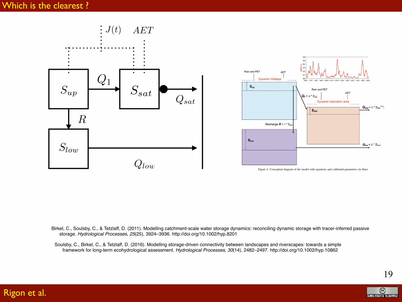
hillslope to the dynamic saturation area in the riparian zoneand underlying groundwater. The approach connects the twoupper storage units which conceptualize storage in theriparian peat soils (Ssat) and the freely draining podzols on thehillslopes (Sup). Direct mapping of the spatial extent ofsaturated soils in the valley bottom – that were hydrologicallyconnected to the stream network during different wetnessconditions (see Ali et al., 2014) – allowed us to develop andfit a simple antecedent precipitation index-type algorithmwhich could explain around >90% of the variability (Birkelet al., 2010). This algorithm was applied to create acontinuous time series of the expanding and contractingdaily saturation area extent (dSAT) (Figure 4). This dSATtime series was used as model input to dynamically distributedaily precipitation inputs between the storage volumes in thelandscape-based (hillslope (Sup) and saturation area (Ssat))model structure (Soulsby et al., 2015).Like Birkel et al. (2015), we used reservoirs that could

become unsaturated allowing storage deficits to occur. Theriparian area is normally saturated (i.e. with positive storage),but can have small deficits following prolonged dry periodsin summer. In the upper stores, water levels below a certainthreshold can only be further depleted by transpiration and nolateral flow to the riparian area will be generated. Incomingprecipitation fluxes arefirst intercepted and reduced by PET –if available. The remaining effective precipitation fills the

uppermost storages and captures soil moisture-relatedthreshold processes of runoff generation (Tetzlaff et al.,2014). Consequently, Sup was often in deficit, but in wetterperiods would fill and spill into Ssat, which usually has low orno deficit generating stream flow.The storages S are state variables in the model, and we

describe the following fluxes and calibrated parametersshown in Figure 4. The unsaturated hillslope reservoir Sup isdrained (fluxQ1 inmmd!1) by a linear rate parameter a (d!1)and directly contributes to the saturation area store Ssat. Therecharge rate R (mm d!1) to groundwater storage Slow islinearly calculated using the parameter r (d!1). The Slow storegenerates runoff Qlow (mm d!1) contributing to totalstreamflow Q (mm d!1) using the linear rate parameter b(d!1). The runoff component Qsat (in mm d!1), which isgenerated nonlinearly from Ssat, conceptualizes saturationoverland flow using the rate parameter k (d!1) and thenonlinearity parameter α (—) in a power function-typeequation (Figure 2).Q is simply the sumofQsat andQlow. Theuse of linear or non-linear parameters was based on priorsystematic tracer-aided multi-model testing for similarcatchments in the Scottish Highlands (Birkel et al., 2010;Capell et al., 2012). In particular, the non-linear conceptu-alization of Qsat has a physical basis in the dynamicexpansion of the saturation area and fluxes that generatestorm runoff. Likewise, the linear nature of Q1 and R reflect

Figure 4. Conceptual diagram of the model with equations and calibrated parameters (in blue)

2487CONNECTIVITY BETWEEN LANDSCAPES AND RIVERSCAPES

Copyright © 2016 The Authors Hydrological Processes Published by John Wiley & Sons Ltd. Hydrol. Process. 30, 2482–2497 (2016)

Take an example of the figure above from Birkel et al. 2011. It pretends to

be explicative and from it we should be able to derive easily the set of mass

conservation that rule the system. However, this action requires a little of

analysis. A more complicate set of reservoirs is shown in the next slide.

Rigon et al.

Introduction

!3

1 Figure 1. Flow diagram for Prediction in Ungauged Basins 2

3

4 Figure 2. Model structure derived from DEM, showing three landscape classes and the 5 groundwater system connecting them. 6

7

β

D

Ks

Kf

Si

Su,max

X

22

Hydrol. Earth Syst. Sci. Discuss., doi:10.5194/hess-2016-433, 2016Manuscript under review for journal Hydrol. Earth Syst. Sci.Published: 29 August 2016c� Author(s) 2016. CC-BY 3.0 License.

Savenije, H. H. G., & Hrachowitz, M. (2016). Opinion paper: How to make our models more physically-based. Hydrology and Earth System Sciences Discussions, 1–23. http://doi.org/10.5194/hess-2016-433

Rigon et al.

Introduction

!4

The idea is to build an algebra of object to represent (water) budgets giving

a clear idea of the type of interactions that the budget is subject to.

Any symbol should correspond to a mathematical term or a group of

mathematical terms. The number and the collocation of parameters of the

models should be clear.

There is a better way to represent reservoir interactions ?

Rigon et al.

Introduction

!5

Mass Conservation

a reservoir. It correspond to a term

a compound reservoir. It represents a set of serial or

parallel reservoirs.

in the l.h.s of water budget equation

A reservoir that can exists depending on some conditions,

e.g. snow

Rigon et al.

Mass

!6

a compound reservoir with sources and sinks.

It represents a set of serial or

parallel reservoirs.

a reservoir with source/sinks. It correspond to a term

in the l.h.s in a water budget equation

and a sink/source term on the r.h.s

This symbol here represents a compound Petri Net

Rigon et al.

Mass Conservation with reactions

!7

a reservoir of energy.

a compound reservoir of energy

a compound reservoir of energy with source/sink of energy, due to chemical reactions, phase transitions or dissipation otherwise specified

Energy Conservation

Rigon et al.

Energy

!8

a reservoir of momentum. It correspond to a term

an assembly of reservoirs where momenta are studied

here loss, acquisition of momentum is described. Loss of momentum comes from friction.

Momentum Conservation

Rigon et al.

Momentum

!9

Sometimes reservoirs can be parametrised, for instance respect substance “age”, then they are represented with shadows

Example of parametrized (ranked) reservoirs

Rigon et al.

Momentum with parametrised subclasses

!10

a reservoir of energy.

a compound reservoir of energy

a compound reservoir of energy with source/sink of energy, due to chemical reactions, phase transitions or dissipation otherwise specified

Adding a gray background means that we have spatial fields

Rigon et al.

Fields of quantities

!11

Eventually we would like to specify discretisation characteristics

1D reservoir. It contains a coordinate. A typical case is when we explicit the width function, or we solve the channel flow with a 1-D de Saint Venant equation.

2D reservoir. It represents a spatial bi-dimensional domain.

3D reservoir. It represents a spatial three-dimensional domain.

Rigon et al.

Discretised fields

!12

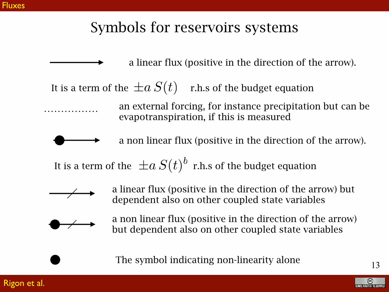
Symbols for reservoirs systems

2D reservoir. It represents a spatial bi-dimensional domain with an unstructured grid.

3D reservoir. It represents a spatial three-dimensional domain with an unstructured grid

Rigon et al.

Discretised fields

!13

Symbols for reservoirs systems

a linear flux (positive in the direction of the arrow).

an external forcing, for instance precipitation but can be evapotranspiration, if this is measured

It is a term of the r.h.s of the budget equation

a non linear flux (positive in the direction of the arrow).

It is a term of the r.h.s of the budget equation

a linear flux (positive in the direction of the arrow) but dependent also on other coupled state variables

a non linear flux (positive in the direction of the arrow) but dependent also on other coupled state variables

The symbol indicating non-linearity alone

Rigon et al.

Fluxes

!14

Symbols for reservoirs systems

In case of a spatially explicit reservoir, this represents von Neumann boundary conditions

In case of a spatially explicit reservoir, this represents Dirichlet boundary conditions

In case of a spatially explicit reservoir, this joins two domains which are solved simultaneously

Rigon et al.

or boundary conditions

!15

Petri Networks

Petri Nets

Rigon et al.

Petri Nets are tools for reprinting chemical reactions. It can be realised that they are perfectly equivalent to our formalism but with different expressivity.

2.2. Standard Petri Net 5

the integration of qualitative, continuous and stochastic information. This allows the representationof di↵erent kinetic processes and di↵erent data types. Petri nets link structural and dynamic analysistechniques to investigate and validate a model such as graph theory, application of linear algebra tocheck a model and simulation methods. This facilitates the performance of simulation studies to explorethe time-dependent dynamic behaviour, the in-depth analysis of structural criteria and the state spaceof a model.

2.2 Standard Petri Net

A Petri net is represented by a directed, finite, bipartite graph, typically without isolated nodes. Thefour main components of a general Petri net are: places, transitions, arcs and tokens; see Figure 2.3,A.

Figure 2.3: Petri Net Formalism. Petri nets consist of places, transitions, arcs and tokens (A). Justplaces are allowed to carry tokens (B). Two nodes of the same type can not be connected with each other(C). The Petri net represents the chemical reaction of the water formation (D). A transition is enabled andmay fire if its pre-places are su�ciently marked by tokens.

Places are passive nodes. They are indicated by circles and refer to conditions or states. In abiological context, places may represent: populations, species, organisms, multicellular complexes,single cells, proteins (enzymes, receptors, transporters, etc.), molecules or ions. But places could alsoembody temperature, pH-value or membrane potential; see also Section 3.3.1. Only places are allowedto carry tokens; see Figure 2.3, B.

Tokens are variable elements of a Petri net. They are indicated as dots or numbers within a placeand represent the discrete value of a condition. Tokens are consumed and produced by transitions; seeFigure 2.3, D. In biological systems tokens refer to a concentration level or a discrete number of aspecies, e.g., proteins, ions, organic and inorganic molecules. Tokens might also represent the value ofphysical quantities like temperature, pH value or membrane voltage that e↵ect biological systems. APetri net without any tokens is called “empty”. The initial marking a↵ects many properties of a Petrinet, which are considered in Chapter 2.

Transitions are active nodes and are depicted by squares. They describe state shifts, system eventsand activities in a network. In a biological context, transitions refer to (bio-)chemical reactions,molecular interactions or intramolecular changes; see also Section 3.3.1. If a place is connected byan arc with a transition, the place (transition) is called pre-place (post-transition). If a transitionis connected by an arc with a place, the transition (place) is called pre-transition (post-place); seeFigure 2.4. Transitions consume tokens from its pre-places and produce tokens within its post-placesaccording to the arc weights; see Figure 2.3, D.

Blätke, M. A., Heiner, M., & Marwan, W. (2011). Petri Nets in System Biology (pp. 1–108). Msgdeburg Universität.

!16

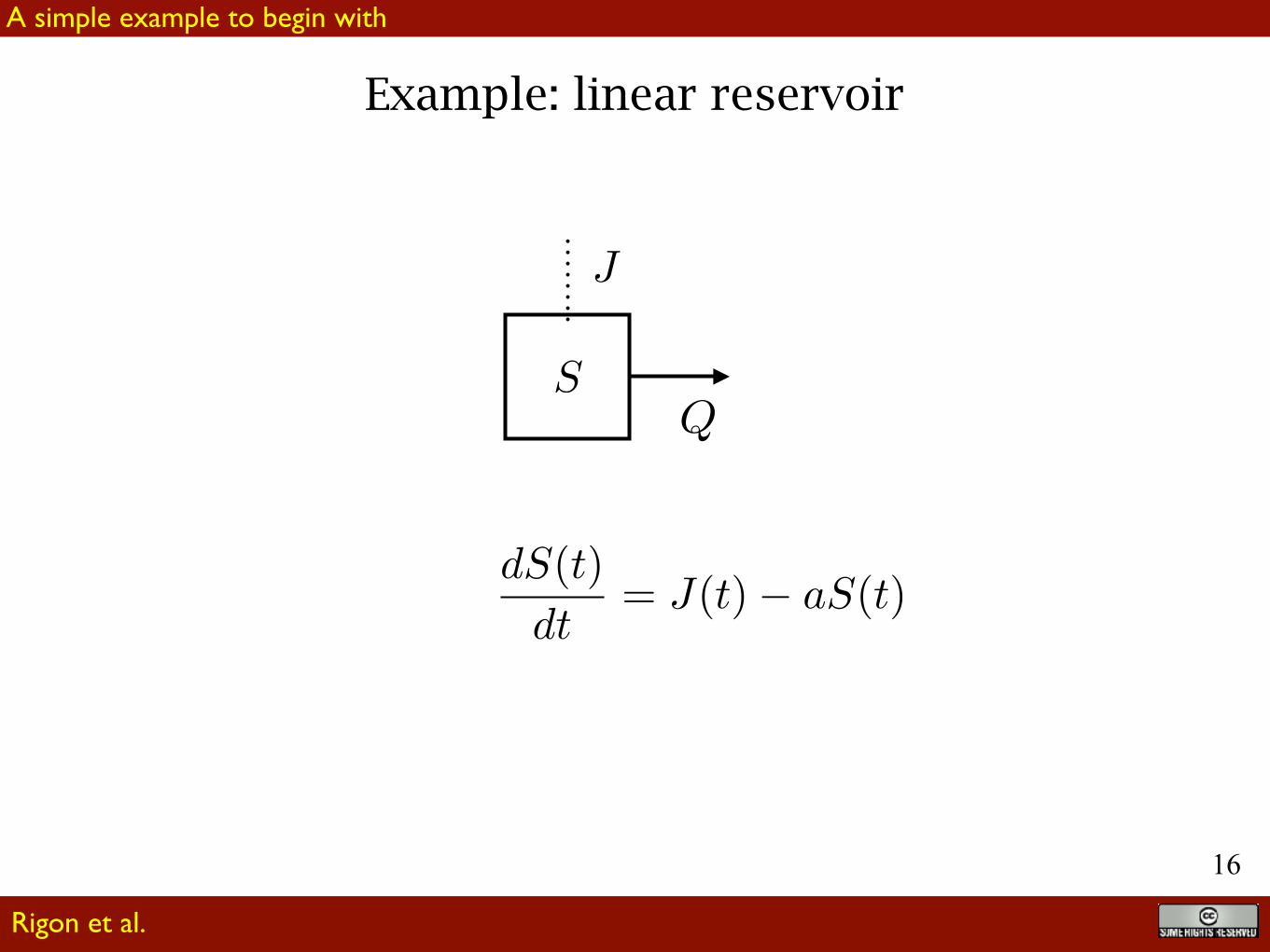
Example: linear reservoir

Rigon et al.

A simple example to begin with

!17

Petri Nets

Rigon et al.

In terms of Petri nets, the same process can be expressed as:

The advantage of using PN would be that there exist several studies about the formal properties of the interactions, that could be eventually used. These studies spans biology, computer science, physics. They were found to be equivalent to Feynman graphs too.

Koch, I. (2014). Petri nets in systems biology. Software & Systems Modeling, 14(2), 703–710. http://doi.org/10.1007/s10270-014-0421-5

!18

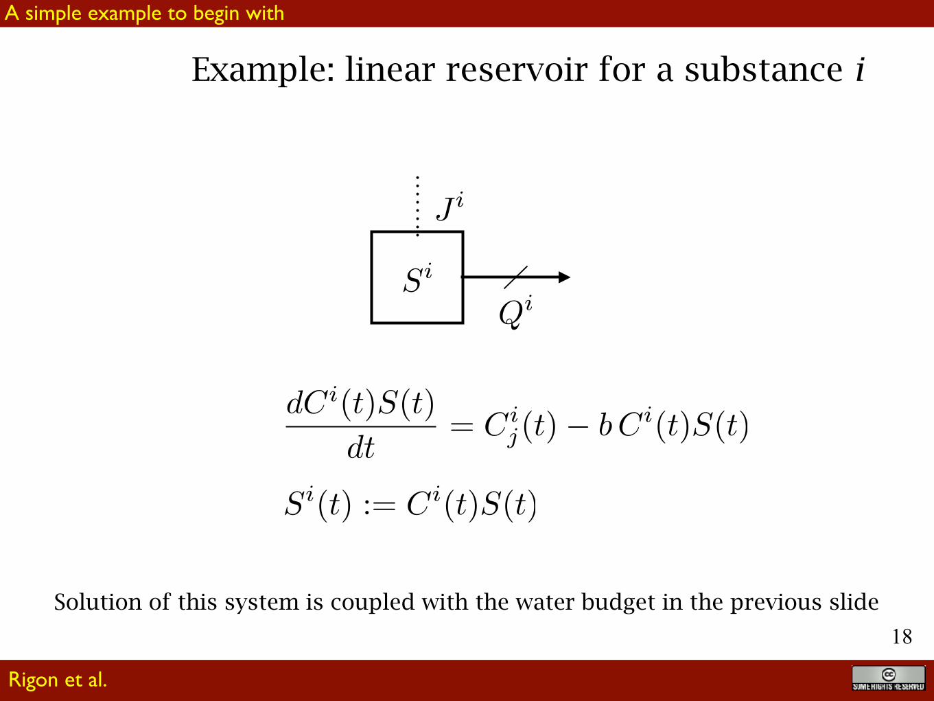
Example: linear reservoir for a substance i

Solution of this system is coupled with the water budget in the previous slide

Rigon et al.

A simple example to begin with

!19

Soulsby, C., Birkel, C., & Tetzlaff, D. (2016). Modelling storage-driven connectivity between landscapes and riverscapes: towards a simple framework for long-term ecohydrological assessment. Hydrological Processes, 30(14), 2482–2497. http://doi.org/10.1002/hyp.10862

hillslope to the dynamic saturation area in the riparian zoneand underlying groundwater. The approach connects the twoupper storage units which conceptualize storage in theriparian peat soils (Ssat) and the freely draining podzols on thehillslopes (Sup). Direct mapping of the spatial extent ofsaturated soils in the valley bottom – that were hydrologicallyconnected to the stream network during different wetnessconditions (see Ali et al., 2014) – allowed us to develop andfit a simple antecedent precipitation index-type algorithmwhich could explain around >90% of the variability (Birkelet al., 2010). This algorithm was applied to create acontinuous time series of the expanding and contractingdaily saturation area extent (dSAT) (Figure 4). This dSATtime series was used as model input to dynamically distributedaily precipitation inputs between the storage volumes in thelandscape-based (hillslope (Sup) and saturation area (Ssat))model structure (Soulsby et al., 2015).Like Birkel et al. (2015), we used reservoirs that could

become unsaturated allowing storage deficits to occur. Theriparian area is normally saturated (i.e. with positive storage),but can have small deficits following prolonged dry periodsin summer. In the upper stores, water levels below a certainthreshold can only be further depleted by transpiration and nolateral flow to the riparian area will be generated. Incomingprecipitation fluxes arefirst intercepted and reduced by PET –if available. The remaining effective precipitation fills the

uppermost storages and captures soil moisture-relatedthreshold processes of runoff generation (Tetzlaff et al.,2014). Consequently, Sup was often in deficit, but in wetterperiods would fill and spill into Ssat, which usually has low orno deficit generating stream flow.The storages S are state variables in the model, and we

describe the following fluxes and calibrated parametersshown in Figure 4. The unsaturated hillslope reservoir Sup isdrained (fluxQ1 inmmd!1) by a linear rate parameter a (d!1)and directly contributes to the saturation area store Ssat. Therecharge rate R (mm d!1) to groundwater storage Slow islinearly calculated using the parameter r (d!1). The Slow storegenerates runoff Qlow (mm d!1) contributing to totalstreamflow Q (mm d!1) using the linear rate parameter b(d!1). The runoff component Qsat (in mm d!1), which isgenerated nonlinearly from Ssat, conceptualizes saturationoverland flow using the rate parameter k (d!1) and thenonlinearity parameter α (—) in a power function-typeequation (Figure 2).Q is simply the sumofQsat andQlow. Theuse of linear or non-linear parameters was based on priorsystematic tracer-aided multi-model testing for similarcatchments in the Scottish Highlands (Birkel et al., 2010;Capell et al., 2012). In particular, the non-linear conceptu-alization of Qsat has a physical basis in the dynamicexpansion of the saturation area and fluxes that generatestorm runoff. Likewise, the linear nature of Q1 and R reflect

Figure 4. Conceptual diagram of the model with equations and calibrated parameters (in blue)

2487CONNECTIVITY BETWEEN LANDSCAPES AND RIVERSCAPES

Copyright © 2016 The Authors Hydrological Processes Published by John Wiley & Sons Ltd. Hydrol. Process. 30, 2482–2497 (2016)

Birkel, C., Soulsby, C., & Tetzlaff, D. (2011). Modelling catchment-scale water storage dynamics: reconciling dynamic storage with tracer-inferred passive storage. Hydrological Processes, 25(25), 3924–3936. http://doi.org/10.1002/hyp.8201

Rigon et al.

Which is the clearest ?

!20

This is the scheme in the previous slide with some small variation

This means that there is a linear flow out out of the upper reservoir (just one parameter). Then the flux is partitioned into two (another parameter).

Rigon et al.

Arguing

!21

Another case

the past developed for and applied at the catchment-scale. Directly adapted from groundwater studies,244

the simplest models rely on a convolution integralapproach, in which input signals are routed throughthe system according to TTDs of predefined functionalshapes.264 This approach is equivalent to hydrologicalmodels based on the instantaneous unit hydro-graph.265 However, the assumptions applied in thesemodels were frequently overly simplistic, includingtime-invariant TTDs, the representation of catchmentsas lumped, completely mixed entities (i.e., using expo-nential distributions as TTD) and inadequate consider-ation of evaporation.256,266 In addition, most of thesestudies merely considered mean TT, which are a ratheruninformative metric.264 Notwithstanding the consid-erable inaccuracies and interpretative biases resultingfrom these assumptions, as demonstrated by severalstudies,267–269 the widespread use of this simplemethod allowed for the development of a sense ofwhich factors do influence the general transport char-acteristics of catchments.270–277 In stepwise improve-ments, studies increasingly moved away from theassumptions of completely mixed systems, in favor ofmore flexible representations that better reflect thenonlinear character of hydrological systems and theimportance of long-tails in the water quality

response.207,216,267,268,275,278 Similarly, the impor-tance of the effect of variable flow conditions on trans-port dynamics, as already emphasized early on,279 haseventually been somewhat embraced by allowing forsome weighting according to the volumes of inputsignals.207,216,280–282 In spite of such advances and theinsights gained, the actual TTDs in these model typesremained, with some rare exceptions,208,283,284 time-invariant and thus implausible representations of real-world systems.

Conceptual ModelsAn alternative, avoiding the most problematicassumptions from the convolution integral method, isthe use of conceptual hydrological models that arecoupled with mixing volumes in their storage compo-nents. Conceptualizing the system as a suite of stor-age components linked by fluxes that represent theperceived dominant processes of a catchment,194 pro-vides a certain degree of flexibility. The possibility tocustomize these models to the environmental condi-tions in a given catchment can ensure an adequatelevel of process heterogeneity to reproduce hydrologi-cal and water quality response patterns of varyingcomplexity.43,285–288

Stream

flow

Stream

flow

Stream

flow

Preferential flow

Preferential flow

Evaporation Evaporation Evaporation

S(t)

ω (t

)

S(t)

ω (t

)

S(t)

ω (t

)

End of dry period,system wet-up

Wet period Begin of dry period

Transpiration Transpiration Transpiration

Precipitation Precipitation

Soilmatrix

Soilmatrix

Soilmatrix

Groundwater GroundwaterGroundwater

(a) (b) (c)

FIGURE 6 | Schematic of changing mixing processes in the soil profile under different wetness conditions with likely shapes of SAS functionsassociated with these conditions. (a) At the end of dry periods, the moisture content in the soil matrix is depleted. Incoming precipitation is, dueto the elevated suction forces relatively quickly adsorbed and stored in the matrix and flow is mainly sustained by relatively old groundwater.(b) As the system wets up, the soil moisture deficits are reduced and less precipitation water enters the matrix, bypassing it, and interacting lesswith the water stored, through preferential flow paths (e.g., root canals, cracks, animal burrows, etc.). Flows are now mainly generated relativelyyoung water reaching the stream for example as preferential flow. (c) At the beginning of a dry period, water stored in the matrix continues torecharge groundwater, further mixing with resident water. Flow is now mainly generated by groundwater, which however, has a higher proportionof younger water than at the end of the dry period.

Overview wires.wiley.com/water

© 2016 The Authors. WIREs Water published by Wiley Periodicals, Inc.

Hrachowitz, M., Benettin, P., van Breukelen, B. M., Fovet, O., Howden, N. J. K., Ruiz, L., et al. (2016). Transit times-the link between hydrology and water quality at the catchment scale. Wiley Interdisciplinary Reviews: Water, 1–29. http://doi.org/10.1002/wat2.1155

Here the description is not unique. It depends on how the percolation is formalised

Rigon et al.

Arguing

!22

Another case

Hrachowitz, M., Benettin, P., van Breukelen, B. M., Fovet, O., Howden, N. J. K., Ruiz, L., et al. (2016). Transit times-the link between hydrology and water quality at the catchment scale. Wiley Interdisciplinary Reviews: Water, 1–29. http://doi.org/10.1002/wat2.1155

This case implies that precipitation goes first into one reservoir and from there is fluxed on the micropore one

This case implies that precipitation is partitioned between the two micropore and macropore reservoirs first

Rigon et al.

Arguing

!23

canopy

rootrunoff

ground

?Snow reservoir is represented as a compound one, since it contains both the water and ice budgets, and an exchange term between the two.

Observe that both canopy and root zone contribute to form the expression of the evapotranspiration flux

snow

Rigon et al.

A possible model scheme with colours

!24

snow

canopy

rootrunoff

ground

Here transpiration depends only on canopy. The flux expression is non linear.

Rigon et al.

A little variation

!25

Single reservoir, coupled mass and energy budget big rows means that the same flux (after appropriate unit conversions) enter the two budgets. A single line means that the flux depends on state variables

Rigon et al.

Coupled equations

!26

Single reservoir, coupled mass and energy budget big rows means that the same flux (after appropriate unit conversions) enter the two budgets. A single line means that the flux depends on state variables. In this case, the water budget is also parametrised (by water ages, for istance).

Rigon et al.

Coupled equations

!27

This is the same model as a few slides above, but solved simultaneously with the water budget. This implies the all the mass fluxes are coupled (because advection of mass is also advection of - latent- energy)

Rigon et al.

A more complex case of interactions

snow

canopy

rootrunoff

ground

JG

!28

A more complicate example interactions

snow

canopy

rootrunoff

ground

Rigon et al.

“G”s represent fluxes by conduction

“J”s or “Q”s represent fluxes by advection

represents coupling with the water budget

“H”s sensible heat

“R”s radiation

!29

Energy and mass conservation together

Rigon et al.

Energy Mass

!30

Conclusion

we hope to have defined a group of signs able to simplify the understanding of reservoir interaction and the way we build our model.

Certainly, this tool has to be still enhanced, but, it is at least a beginning.

Rigon et al.

Questions ?

!31

Find this presentation at

http://abouthydrology.blogspot.com

Ulr

ici, 2

00

0 ?

Other material at

Domande

Rigon et al.