MCA_UNIT-1_Computer Oriented Numerical Statistical Methods

Course: MCASubject: Computer Oriented Numerical

Statistical MethodsUnit-1

RAI UNIVERSITY, AHMEDABAD

RAI UNIVERSITY, AHMEDABAD 1

Unit-I- Solution of Non-linear Equations

Sr.

No.

Name of the Topic Page

No.

1 Absolute, Relative and Percentage Error 1

2 Roots of an equation, Linear and non-Linear equations

(Definition and Difference),

4

3 Iterative Methods for finding roots of non-Linear equations :

Bisection Method

5


Newton-Raphson Method

14


False Position Method

18


secant Method

25

7 Exercise 29

8 References 30


1.1 Errors

In practice, all measurements are subject to errors and it is therefore of importance

to find the total effect of small errors in the observed values of the variables, on a

quantity which depends on these variables.

If δx is an error in X then

|δx|=|True value−Approximate value| is called an absolute error in X ,

δxx

is called the relative error in X and

δxx

× 100 is called the percentage error in X .

Example—

A circle of radius r=5 cm having an error in radius 10 % ,then find percentage

error in its area.

Solution:

Area of circle A=π r2

∴ A=π r2 ⇒ δA=2πrδr

Now δAA

=2 πrδr

π r2

δAA

=2 δrr

∴ δAA

× 100=2 ( δrr

× 100) ∴ δA

A× 100=2 (10 )

∴ δAA

× 100=20

Therefore percentage error in Area of circle is 20.

Example—


A cuboid having error in their sides equal to 2 % , 5 %∧1 % . Then find the

corresponding error in its volume.

Solution:

Volume of cuboid is V=l × w ×h

δV =whδl+ lhδw+wlδh

Now we have to given that, l=2 % , w=5 % , h=1 %

δVV

=whδl+lhδw+wlδhl × w ×h

δVV

×100=( δll+ δh

h+ δw

w )×100

δVV

×100=( δll

×100)+( δhh

× 100)+( δww

×100) δVV

×100=2+5+1

δVV

×100=8

Error in Volume of cuboid = 8 %

Example—

A right circular cone of radius r=10 cm∧h=20 cm having percentage error in

radius equal to 1 % and percentage error in height equal to 5 % then find

(i) Absolute error

(ii) Relative error

(iii) Percentage error

in the volume of right circular cone.

Solution:

Volume of right circular cone

V=13

π r2 h

δV =13

2 rδrh+13

π r 2δh


Now we have to given that r=10 cm, h=20 cm ,δrr

×100=1 ,δhh

×100=5

δr=1× r100

¿δh=5 ×h100

δV =13

π [2×r × h×( 1× r100 )+r 2( 5× h

100 )] δV =1

3π [2×10 ×20 ×

1 ×10100

+10 × 10× 5× 20100 ]

δV =13

π [ 40+100 ]

δV =13

π [140]

δV =146.53

∴Absolute error δV =146.53

⇒ δVV

=146.5313

π r2 h= 3 × 146.53

π ×100 × 20

∴ δVV

=439.596283

=0.06996≅ 0.07

∴ Relative error δVV

=0.07

δVV

×100=0.07 ×100=7

∴ Percentage error = 7 %

2.1 Linear equation— General form of a linear equation is—

ax+by=c, where a ,b∧c are constants.

2.2 Graph of a linear equation— An equation ax+by=c represents a straight line.

2.3 Solution of two linear equations— Solution of two linear equations

a1 x+b1 y=c1 and a2 x+b2 y=c2 is given by—

x=c1 b2−c2b1

a1 b2−a2 b1 and y=

c2a1−c1a2

a1b2−a2 b1.


Graphically this solution gives the point of intersection of these straight lines.

Example—

Find the solution of the equations x+2 y=3 and3 x+ y=4.

Solution— given straight lines are x+2 y=3 and3 x+ y=4.

Here, a1=1 ,b1=2 , c1=3 , a2=3 , b2=1 , c2=4

Hence, x=c1 b2−c2b1

a1 b2−a2 b1

=3.1−4.21.1−3.2

=3−81−6

=1 and y=c2a1−c1a2

a1b2−a2 b1

=4.1−3.31.1−3.2

=4−91−6

=1

2.4 Definition: Non-linear equation:

A polynomial of degree at least 2 is called nonlinear equation.

Graph of a non-linear equation is not a straight line.

e.g.x3−3 x+1=0, cosx−xe x=0.

2.5 Here we use Numerical Methods for solving Non-linear equations like

Bisection Method

Regula-Falsi Method

Newton-Raphson Method

Secant Method

3.1 Introduction—

In the Applied mathematics and engineering the problem of determining the roots

of an equation f (x)=0 has a great importance.

If f (x) is a polynomial of degree two or more , we have formulae to find

solution. But, if f(x) is a transcendental function, we do not have formulae to

obtain solutions. When such type of equations are there, we have some


methods like Bisection method, Newton-Raphson Method and The method

of false position. Those methods are solved by using a theorem in theory of

equations, i.e., “If f(x) is continuous in the interval (a ,b)and if f (a) and f (b)

are of opposite signs, then the equation f (x)=0 will have at least one real

root between aand b”.

3.2 Definition—

A number ξ is a solution of f (x)=0 if f (ξ)=0 . Such a solution ξ is a root of f (x)=0.

3.3 Iterative Method—

This method is based on the idea of successive approximation.i.e. Starting with one

or more initial approximations to the root, we obtain a sequence of approximations

or iterates {xk } , which in the limit converges to the root.

Definition—

A sequence of iterates {xk } is said to converge to the root ξ, if

limk⟶∞

|xk−ξ|=0∨ limk⟶∞

xk=ξ.

3.4 Bisection Method—

Let us suppose we have an equation of the form f (x)=0 in which solution lies

between in the range (a ,b) .

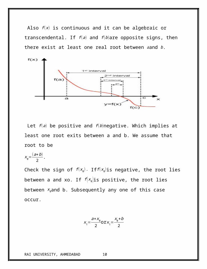
Also f (x) is continuous and it can be algebraic or transcendental. If f (a) and f (b)

are opposite signs, then there exist at least one real root between aand b.


Let f (a) be positive and f (b)negative. Which implies at least one root exits

between a and b. We assume that root to be

x0=(a+b)

2.

Check the sign of f (x0) . Iff (x0)is negative, the root lies between a and xo. If f ( x0 )is

positive, the root lies between x0and b. Subsequently any one of this case occur.

x1=a+x0

2orx1=

x0+b

2

When f (x¿¿1)¿is negative, the root lies between x0and x1 and let the root be

x2=x0+x1

2. Againf (x¿¿2)¿negative then the root lies between x0and x2, let x3=

x1+x2

2

and so on.

Repeat the processx0,x1, x2 , …Whose limit of convergence

is the exact root.

3.5 Steps—


1. Find a and b in which f(a) and f(b) are opposite signs for the given equation

using trial and error method.

2. Assume initial root as

x0=(a+b)

2

3. Iff (x0) is negative, the root lies between a and x0 . And takes the root as

x1=(a+ x0)

2

4. Iff (x0)is positive, then the root lies between x0 and b.And takes the root as

x1=(x0+b)

2

5. Iff (x1) is negative, the root lies between x0and x1 . And takes the root as

x2=(x0+x1)

2

6. Iff (x1) is positive, the root lies between x0and x2 . And takes the root as

x2=(x0+x2)

2

7. Repeat the process until any two consecutive values are equal and hence the

root.

This method is simple to use and the sequence of approximations always

converges to the root for any f (x) which is continuous in the interval that contains

the root.


If the permissible error isε, then the approximation number of iteratives required

may be determined from the relationb0−a0

2n ≤ ε.

The minimum number of iterations required for converging to a root in the interval

(0,1) for a given ε are listed as

Number of iterations

ε 10−2 10−3 10−4 10−5 10−6 10−7

n 7 10 14 17 20 24

The bisection method requires a large number of iterations to achieve a reasonable

degree of accuracy of the root. It requires one function at each iteration.

Example—

Find the positive root of x3−x=1correct to four decimal places by bisection

method.

Solution—

Let f ( x )=x3− x−1

f (0 )=03−0−1=−1=−ve

f (1 )=13−1−1=−1=−ve

f (2 )=23−2−1=5=+ve

So the root lies between the 1 and 2.

We can take x0=1+2

2=3

2=1.5 as initial root and proceed.

i.e.,f (1.5)=0.8750=+ve

andf (1)=−1=−ve

So the root lies between 1 and 1.5.


x1=1+1.5

2=2.5

2=1.25

as initial root and proceed.

f (1.25)=−0.2969

So the root x2lies between 1.25 and 1.5.

Now

x2=1.25+1.5

2=2.75

2=1.3750

f (1.375)=0.2246=+ve

So the root x3lies between 1.25 and 1.375.

Now

x3=1.25+1.3750

2=2.6250

2=1.3125

f (1.3125)=−0.051514=−ve

Therefore, root lies between 1.375and 1.3125

Now

x4=(1.375+1.3125)/2=1.3438

f (1.3438)=0.082832=+ve

So root lies between 1.3125 and 1.3438

Now

x5=(1.3125+1.3438)/2=1.3282

f (1.3282)=0.014898=+ve


Now

x6=(1.3125+1.3282)/2=1.3204


f (1.3204)=−0.018340=−ve


Now

x7=(1.3204+1.3282)/2=1.3243

f (1.3243)=−ve

So root liesbetween 1.3243and 1.3282

Now

x8=(1.3243+1.3282)/2=1.3263

f (1.3263)=+ve


Now

x9=(1.3243+1.3263)/2=1.3253

f (1.3253)=+ve


Now

x10=(1.3243+1.3253) /2=1.3248

f (1.3248)=+ve


Now

x11=(1.3243+1.3248)/2=1.3246

f (1.3246)=−ve


Now


x12=(1.3248+1.3246) /2=1.3247

f (1.3247)=−ve


Now

x13=(1.3247+1.3247)/2=1.32475

Hence the approximate root is 1.32475 .

Example—

Find the positive root of x – cos x=0 by bisection method.

Solution—

Let

f ( x )=x – cos x , f (0)=0−cos (0)=0−1=−1=−ve

f (0.5)=0.5 – cos(0.5)=−0.37758=−ve

f (1)=1 – cos (1)=0.42970=+ve

So root lies between 0.5 and 1

Let

x0=(0.5+1 )

2=0.75

as initial root and proceed.

f (0.75)=0.75 – cos(0.75)=0.018311=+ve


x1=(0.5+0.75)/2=0.62

f (0.625)=0.625 – cos(0.625)=−0.18596


x2=(0.625+0.750)/2=0.6875


f (0.6875)=−0.085335


x3=(0.6875+0.750)/2=0.71875

f (0.71875)=0.71875−cos (0.71875)=−0.033879


x4=(0.71875+0.750) /2=0.73438

f (0.73438)=−0.0078664=−ve


x5=0.742190

f (0.742190)=0.0051999=+ve

x6=(0.73438+0.742190)/2=0.73829

f (0.73829)=−0.0013305


x7=(0.73829+0.74219)=0.7402

f (0.7402)=0.7402

cos (0.7402)=0.0018663


x8=0.73925

f (0.73925)=0.00027593

x9=0.7388

The root is 0.7388.

3.6 Advantages of bisection method—

a) The bisection method is always convergent. Since the method brackets the

root, the method is guaranteed to converge.

b) As iterations are conducted, the interval gets halved. So one can guarantee

the error in the solution of the equation.


3.7 Drawbacks of bisection method—

a) The convergence of the bisection method is slow as it is simply based on

halving the interval.

b) If one of the initial guesses is closer to the root, it will take larger number of

iterations to reach the root.

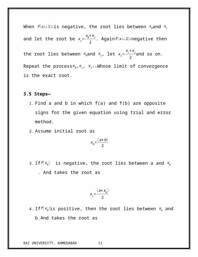
4.1 Newton-Raphson method (or Newton’s method)—

Suppose we have an equation of the form f (x)=0, whose solution lies between the

range(a , b ) .Also f (x)is continuous and it can be algebraic or transcendental. If f (a)

and f (b)are opposite signs, then there exist at least one real root between aand b.

Let f (a)be positive and f (b)negative. Which implies at least one root exits in

between aand b. We assume that root to be either a or b, in which the value of

f (a)orf (b) is very close to zero. That number is assumed to be initial root. Then we

iterate the process by using the following formula until the value is converges.

xn+1=xn−f (xn)f ' (xn)

4.2 Steps—

1. Find aand b in whichf (a)and f (b) are opposite signs for the given equation



2. Assume initial root as x0=a i.e., if f (a)is very close to zero or x0=b iff (a)is

very close to zero.

3. Find x1 by using the formula

x1=x0−f (x0)f ' (x0)

4. Find x2 by using the following formula

x2=x1−f ( x1 )f ' ( x1 )

5. Find x3 , x4 , . .. xn until any two successive values are equal .

Example 1—

Find the positive root of f (x)=2x3−3 x−6=0 by Newton – Raphson method

correct to five decimal places.

Solution—

Letf (x)=2x3−3 x – 6 ; f ' (x)=6 x2 – 3

xn+1=xn−f ( xn )f ' ( xn )

=xn−2 xn

3−3 xn –6

6 xn2 – 3

=(6 xn

3−3 xn) – (2 xn3−3 xn – 6)

6 xn2 – 3

=6 xn

3−3 xn – 2xn3+3 xn+6

6 xn2 – 3

=4 xn

3+6

6 xn2 – 3

f (1)=2−3−6=−7=−ve

f (2)=16 – 6−6=4=+ve

So, a root between 1 and 2 .

In which 4 is closer to 0. Hence we assume initial root as 2.

Consider x0=2

So


x1=4 x0

3+6

6 x02 –3

= 4 × 23+66× 22−3

=3821

=1.809524

x2=(4 (1.809524 )3+6)/(6 (1.809524 )2−3)=29.700256 /16.646263=1.784200

x3=(4 (1.784200 )3+6) /(6 (1.784200 )2−3)=28.719072/16.100218=1.783769

x4=(4 (1.783769 )3+6)/(6 (1.783769 )2−3)=28.702612/16.090991=1.783769

Since x3 and x4 are equal, hence root is 1.783769 .

Example 2—

Using Newton’s method, find the root between 0 and 1 of x3=6 x – 4 correct to 5

decimal places.

Solution—

Letf ( x )=x3−6 x+4

xn+1=xn−f ( xn )f ' ( xn )

¿ xn−xn

3−6 xn+4

3 xn2−6

=(3 x¿¿n¿¿3−6 xn)−(xn

3−6 xn+4 )3 xn

2−6¿¿

¿3 xn

3−6 xn−xn3+6 xn−4

3 xn2−6

=2 xn

3−4

3 xn2−6

f (0 )=4=+ve; f (1)=−1=−ve

So a root lies between 0 and 1

f (1)is nearer to 0. Therefore we take initial root as x0=1

x1=2 xn

3−4

3 xn2−6

=2 ×13−43 ×12−6

=2−43−6

=−2−3

=0.66666


x2=(2 (0.66666 )3 – 4) /(3 (0.66666 )2−6)=0.73016

x3=(2 (0.73015873 )3 – 4)/ (3 (0.73015873 )2−6)=(3.22145837 /4.40060469)=0.73205

x4=(2 (0.73204903 )3 – 4)/(3 (0.73204903 )2−6)=(3.21539602/4.439231265)=0.73205

The root is 0.73205 correct to 5 decimal places.

4.3 Advantages of Newton Raphson method—

Fast convergence!

4.4 Disadvantages of Newton Raphson method—

a) May not produce a root unless the starting value x0 is close to the actual root

of the function.

b) May not produce a root if for instance the iterations get to a pointxn−1such that

f ' ( xn−1 )=0 . then the method is false.

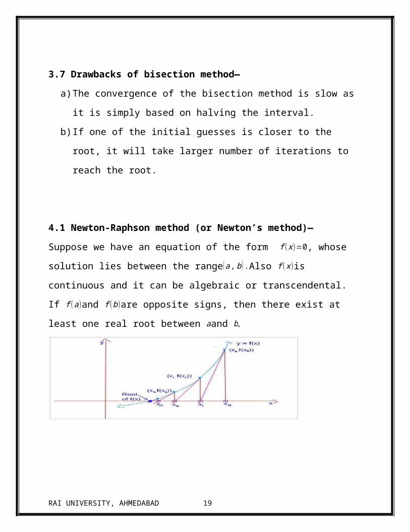
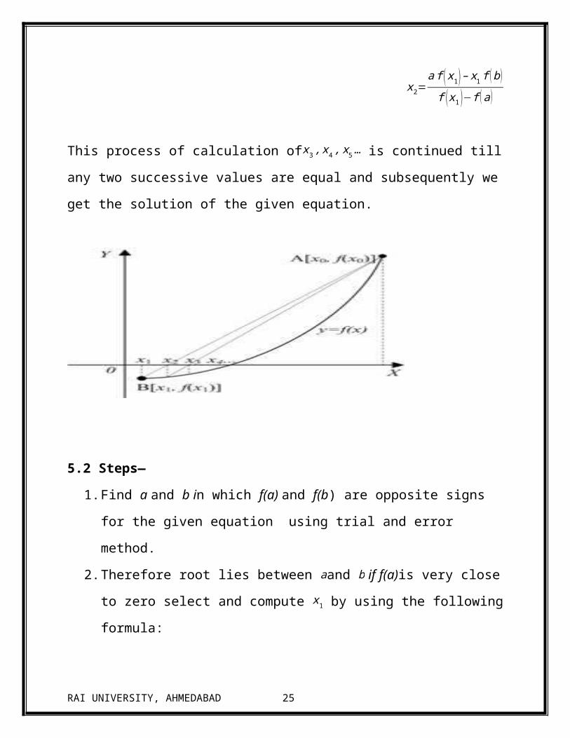
5.1 Method of False Position ( or RegulaFalsi Method )—

Let us consider the equation f (x)=0and f (a) and f (b) are of opposite signs. Also let

a<b .

The graph y=f (x ) will meet the x-axis at some point between A(a , f (a)) and

B(b , f (b)).The equation of the chord joining the two points A(a , f (a)) and B(b , f (b))

is

y – f (a)x−a

=f (a)−f (b)

a−b

The x- Coordinate of the point of intersection of this chord with the x-axis gives an

approximate value for the of f (x)=0. Taking y = 0 in the chord equation, we get

– f (a)x−a

=f (a)−f (b)

a−b

⟹ x [ f (a)−f (b)]−a f (a)+a f (b)=−a f (a)+b f (a)

⟹ x [ f (a )−f (b ) ]=b f (a )−a f ( b )


⟹ x=b f (a )−a f ( b ) ;

f (a )−f (b )

This x1gives an approximate value of the root (x )=0.(a<x1<b) .

Now f (x1) and f (a) are of opposite signs or f (x1) and f (b) are opposite signs.

Iff ( x1 ) . f (a)<0 . Then x2 lies between x1 and a.

x2=a f ( x1 ) – x1 f (b )

f ( x1 )−f (a )

This process of calculation ofx3 , x4 , x5… is continued till any two successive values

are equal and subsequently we get the solution of the given equation.

5.2 Steps—

1. Find a and b in which f(a) and f(b) are opposite signs for the given equation



2. Therefore root lies between aand b if f(a)is very close to zero select and

compute x1 by using the following formula:

x1=af (b )−bf (a)

f (b )−f (a)

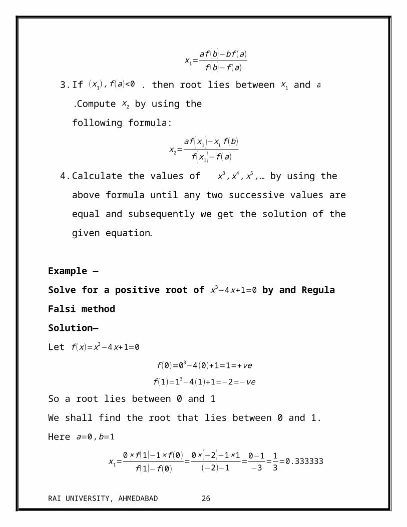
3. If (x1) , f (a)<0 . then root lies between x1 and a .Compute x2 by using the

following formula:

x2=af ( x1)−x1 f (b)

f ( x1 )−f (a)

4. Calculate the values of x3 , x4 , x5 ,… by using the above formula until any two

successive values are equal and subsequently we get the solution of the

given equation.

Example —

Solve for a positive root of x3−4 x+1=0 by and Regula Falsi method

Solution—

Let f (x)=x3−4 x+1=0

f (0)=03−4 (0)+1=1=+ve

f (1)=13−4(1)+1=−2=−ve

So a root lies between 0 and 1

We shall find the root that lies between 0 and 1.

Here a=0 , b=1

x1=0 ×f (1 )−1× f (0)

f (1 )−f (0)=

0 × (−2 )−1× 1(−2)−1

=0−1−3

=13=0.333333

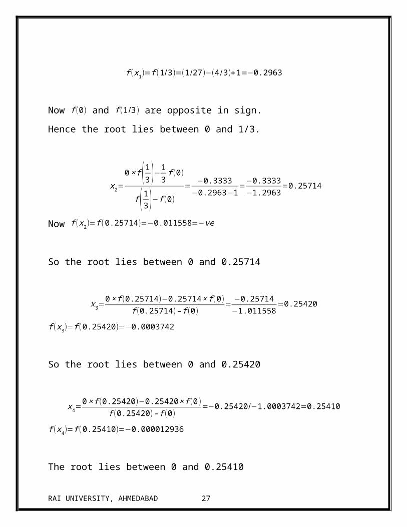
f (x1)=f (1/3)=(1/27)−(4 /3)+1=−0.2963

Now f (0) and f (1/3) are opposite in sign.

Hence the root lies between 0 and 1/3.


x2=0 × f ( 1

3 )−13

f (0)

f ( 13 )−f (0)

= −0.3333−0.2963−1

=−0.3333−1.2963

=0.25714

Now f (x2)=f (0.25714 )=−0.011558=−ve

So the root lies between 0 and 0.25714

x3=0 × f (0.25714)−0.25714 × f (0)

f (0.25714 )– f (0)= −0.25714

−1.011558=0.25420

f (x3)=f (0.25420)=−0.0003742

So the root lies between 0 and 0.25420

x4=0 × f (0.25420)−0.25420 × f (0)

f (0.25420)– f (0)=−0.25420/−1.0003742=0.25410

f (x4)=f (0.25410)=−0.000012936

The root lies between 0 and 0.25410

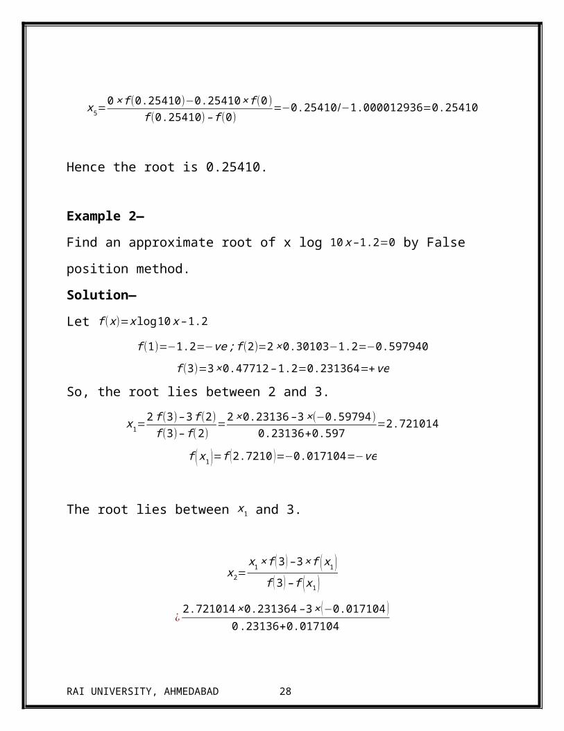
x5=0 × f (0.25410)−0.25410 × f (0)

f (0.25410)– f (0)=−0.25410/−1.000012936=0.25410

Hence the root is 0.25410.

Example 2—

Find an approximate root of x log 10 x – 1.2=0 by False position method.

Solution—


Let f (x)=x log 10 x – 1.2

f (1)=−1.2=−ve; f (2)=2×0.30103−1.2=−0.597940

f (3)=3 ×0.47712 –1.2=0.231364=+ve

So, the root lies between 2 and 3.

x1=2 f (3)– 3 f (2)

f (3)– f (2)=

2× 0.23136 – 3×(−0.59794 )0.23136+0.597

=2.721014

f ( x1 )=f (2.7210 )=−0.017104=−ve

The root lies between x1 and 3.

x2=x1 × f (3 ) – 3× f ( x1 )

f (3 ) – f ( x1 )

¿2.721014 ×0.231364 – 3× (−0.017104 )

0 .23136+0.017104

¿ 0.629544+0.0513120.24846

=0.6808560.248464

=2.740260

f ( x2 )=f (2.7402 )=2.7402 × log (2.7402 ) – 1.2=−0.00038905=−ve

So the root lies between 2.740260 and 3.

x3=2.7402× f (3) – 3× f (2.7402)

f (3) – f (2.7402)=

2.7402 x 0.231336+3 x (0.00038905)0.23136+0.00038905

=0.635140.23175

=2.740627

f ( x3 )=f (2.7406 )=0.00011998=+ve

So the root lies between 2.740260 and 2.740627

x4=2.7402 x f (2.7406) – 2.7406 x f (2.7402)

f (2.7406) – f (2.7402)=2.7402 x 0.00011998+2.7406 x 0.00038905

0.00011998+0.00038905= 0.0013950

0.00050903=2.7405


Hence the root is 2.7405.

5.3 Advantages of RegulaFalsi Method—

No need to calculate a complicated derivative (as in Newton's method).

5.4 Disadvantages of RegulaFalsi Method—

a) May converge slowly for functions with big curvatures.

b) Newton-Raphson may be still faster if we can apply it.

5.5 Rate Of Convergence —

Here we discuss the rate at which the iteration method converges if the initial

approximation to the root is sufficiently close to the desired root.

5.5.1Definition—

An iterative method is said to be of order p or has the rate of convergence p, if p is

the largest positive real number for which there exists a finite constant C ≠ 0 such

that

|εk+1|≤ C|εk|p

Where ε k=xk−ξ is the error in the kth iteratation. The constant C is called the

asymptotic error constant and usually depends on the derivative of f (x) atx=ξ.

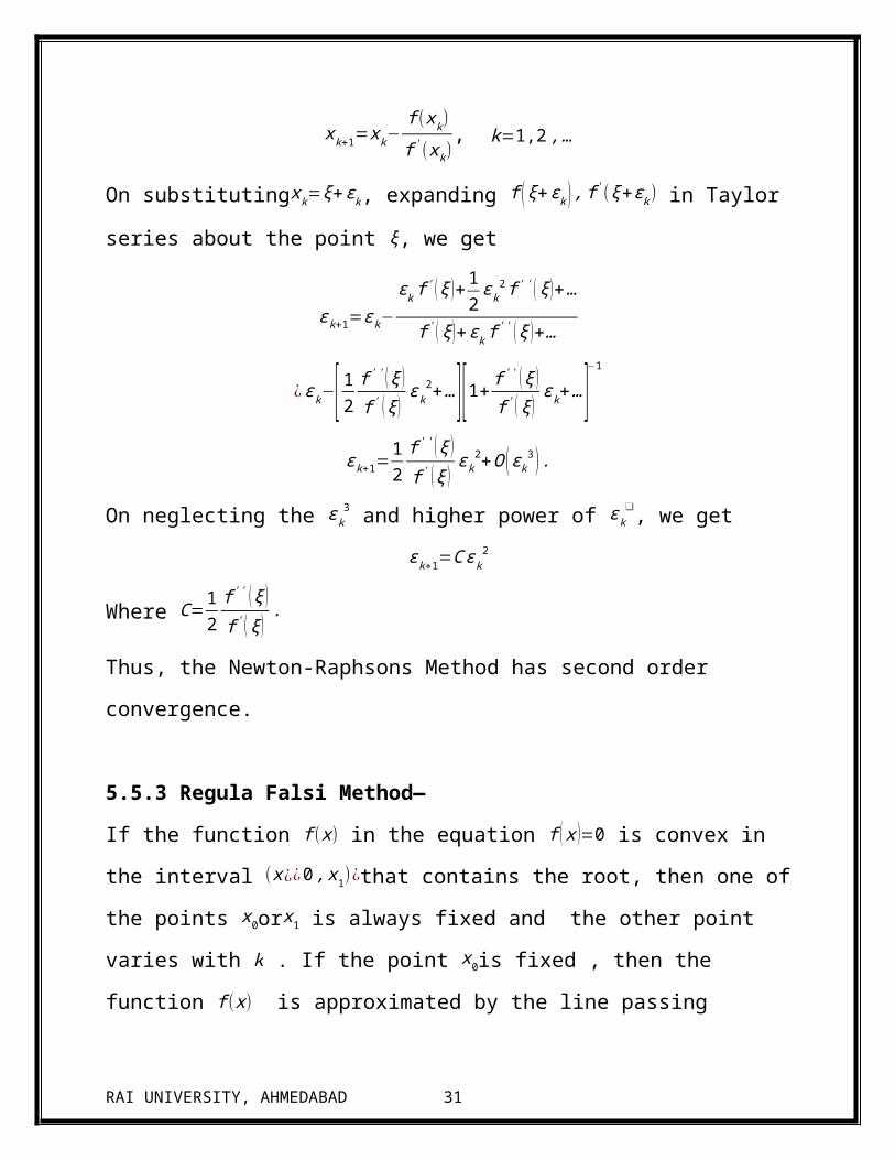
5.5.2 Newton-Raphsons Method—

We know

xk+1=xk−f ( xk)f ' (xk)

, k=1,2 , …


On substitutingxk=ξ+εk, expanding f ( ξ+εk ) , f ' (ξ+εk) in Taylor series about the point

ξ, we get

ε k+1=εk−ε k f ' (ξ )+ 1

2ε k

2 f ' ' (ξ )+…

f ' (ξ )+εk f ' ' (ξ )+…

¿ ε k−[ 12

f ' ' (ξ )f ' (ξ )

εk2+…] [1+

f ' ' (ξ )f ' (ξ )

εk+… ]−1

ε k+1=12

f ' ' (ξ )f ' (ξ )

εk2+O (ε k

3) .

On neglecting the ε k3 and higher power of ε k

❑, we get

ε k+1=C εk2

Where C=12

f ' ' (ξ )f ' (ξ )

.

Thus, the Newton-Raphsons Method has second order convergence.

5.5.3 Regula Falsi Method—

If the function f (x) in the equation f ( x )=0 is convex in the interval (x¿¿0 , x1)¿that

contains the root, then one of the points x0orx1 is always fixed and the other point

varies with k . If the point x0is fixed , then the function f (x) is approximated by the

line passing through the points (x0 , f (x0)) and (xk , f (xk )) , k=1,2,3 ,… the error of the

equation becomes

ε k+1=C ε0 εk

Where C=12

f ' ' (ξ )f ' (ξ )

and ε 0=x0−ξ is independent of k . Therefore we can write

ε k+1=C ¿ε k

Where C ¿=C ε0 is the asymptotic error constant. Hence the Regula-Falsi method has

linear rate of convergence.

6.1 Secant Method


Although the Newton-Raphson method is very power full to solve non-linear

equations, evaluating of the function derivative is the major difficulty of this

method. To overcome this deficiency, the secant method starts the iteration by

employing two starting points and approximates the function derivative by

evaluating of the slope of the line passing through these points. The secant method

has been shown in Fig. 1. As it is illustrated in Fig. 1, the new guess of the root of

the function f(x) can be found as follows:

In the first glance, the secant method may be seemed similar to linear interpolation

method, but there is a major difference between these two methods. In the secant


method, it is not necessary that two starting points to be in opposite sign.

Therefore, the secant method is not a kind of bracketing method but an open

method. This major difference causes the secant method to be possibly divergent in

some cases, but when this method is convergent, the convergent speed of this

method is better than linear interpolation method in most of the problems.

The algorithm of the secant method can be written as follows:

6.2 Steps—

Step 1: Choose two starting points x0 and x1.

Step 2: Let

Step 3: if |x2-x1|<e then let root = x2, else x0 = x1 ; x1 = x2 ; go to step 2.

Step 4: End.

e: Acceptable approximated error.

Example—

A Real root of the equation f ( x )=x3−5x+1=0 lies in the interval (0,1 ) . Perform

four iterations of the secant method.

Solution:

We have x0=0 , x1=1 , f 0=f ( x0 )=1 , f 1=f ( x1 )=−3

x2=x1−[ x0−x1

f 0−f 1] f 1=1−[ 0−1

1+3 ] (−3 )=1−34=0.25

f 2=f ( x2 )=f (0.25 )=−0.234375

x3=x2−[ x1−x2

f 1−f 2]=0.186441


http://www.numericmethod.com/About-numerical-methods/roots-of-equations/secant-method/Eq2.jpg?attredirects=0

∴ f 3=f ( x3)=0.074276

x4=x3−[ x3−x2

f 3−f 2] f 3=0.201736

∴ f 4=f ( x4 )=−0.000470

x5=x4−[ x 4−x3

f 4−f 3] f 4=0.201640

6.3 Advantages of secant method:

1. It converges at faster than a linear rate, so that it is more rapidly

convergent than the bisection method.

2. It does not require use of the derivative of the

function, something that is not available in a number

of applications.

3. It requires only one function evaluation per iteration,

as compared with Newton’s method which requires

two.

6.4 Disadvantages of secant method:

1. It may not converge.

2. There is no guaranteed error bound for the computed

iterates.

3. It is likely to have difficulty if f 0(α)=0. This

means the x-axis is tangent to the graph of y=f (x )atx=α .4. Newton’s method

generalizes more easily to new

methods for solving simultaneous systems of nonlinear

equations.


EXERCISE

Que—Solve the following Examples:

1. Find a positive root of the following equation by bisection method :

x3−4 x−9

( Answer :2.7065)

2. Solve the following by using Newton – Raphson Method :x3 – x−1

( Answer :1.3247)3. Solve the following by method of false position (RegulaFalsi Method) :

x3+2 x2+10 x – 20( Answer :1.3688)

4. Solve the following equation by Secant Method up to four iteration.

cosx−xe x=0 in interval (0,1).


(Answer :0.5317058606 ¿

REFERENCES

1. Numerical Method for Science and Computer science by M.K. Jain, S.R.K.

Iyenger, R.K. Jain

2. http://www.google.co.in/url?

sa=t&rct=j&q=&esrc=s&source=web&cd=2&ved=0CCMQFjAB&url=http

%3A%2F%2Fwww.b-u.ac.in%2Fsde_book

%2Fbca_numer.pdf&ei=uKenVMatGceduQTt9ILwBw&usg=AFQjCNH7o

ooXkwN7zusFPiJS7MksUkmZaw&bvm=bv.82001339,d.c2E&cad=rja

3. http://1.bp.blogspot.com/_BqwTAHDIq4E/TCqWRUqn7qI/

AAAAAAAAACE/oe-W-JZaQRI/s400/Dibujo.bmp

4. http://www.google.co.in/imgres?imgurl=http%3A%2F

%2Fimage.tutorvista.com%2Fcms%2Fimages%2F39%2Fnewton

%252513raphson-method.JPG&imgrefurl=http%3A%2F

%2Fmath.tutorvista.com%2Fcalculus%2Fnewton-raphson-

method.html&h=283&w=500&tbnid=VCvTr-sjzqmjDM

%3A&zoom=1&docid=o_YQeEzCa1CVHM&ei=B6SnVMCEDomlNqbsga


http://www.google.co.in/imgres?imgurl=http%3A%2F%2Fimage.tutorvista.com%2Fcms%2Fimages%2F39%2Fnewton%252513raphson-method.JPG&imgrefurl=http%3A%2F%2Fmath.tutorvista.com%2Fcalculus%2Fnewton-raphson-method.html&h=283&w=500&tbnid=VCvTr-sjzqmjDM%3A&zoom=1&docid=o_YQeEzCa1CVHM&ei=B6SnVMCEDomlNqbsgaAN&tbm=isch&ved=0CB0QMygBMAE&iact=rc&uact=3&dur=4533&page=1&start=0&ndsp=17


http://1.bp.blogspot.com/_BqwTAHDIq4E/TCqWRUqn7qI/AAAAAAAAACE/oe-W-JZaQRI/s400/Dibujo.bmp

http://1.bp.blogspot.com/_BqwTAHDIq4E/TCqWRUqn7qI/AAAAAAAAACE/oe-W-JZaQRI/s400/Dibujo.bmp

http://www.google.co.in/url?sa=t&rct=j&q=&esrc=s&source=web&cd=2&ved=0CCMQFjAB&url=http%3A%2F%2Fwww.b-u.ac.in%2Fsde_book%2Fbca_numer.pdf&ei=uKenVMatGceduQTt9ILwBw&usg=AFQjCNH7oooXkwN7zusFPiJS7MksUkmZaw&bvm=bv.82001339,d.c2E&cad=rja



AN&tbm=isch&ved=0CB0QMygBMAE&iact=rc&uact=3&dur=4533&pag

e=1&start=0&ndsp=17

5. http://www.google.co.in/url?

sa=i&rct=j&q=&esrc=s&source=images&cd=&cad=rja&uact=8&ved=0CA

cQjRw&url=http%3A%2F%2Fmathumatiks.com%2Fsubpage-373-Regula-

Falsi-Method.htm&ei=6aWnVK-

1Eo3muQSuqILABg&bvm=bv.82001339,d.eXY&psig=AFQjCNGE5QOy

UayJysWeiBMOzx7QBybl_w&ust=1420359120049725

6. http://www.numericmethod.com/About-numerical-methods/roots-of-

equations/secant-method

7. http://www.dummies.com/how-to/content/how-to-solve-nonlinear-

systems0.html

8. http://studyhelpszone.blogspot.in/2009/07/advantages-and-disadvanteges-of-

secant.html


http://studyhelpszone.blogspot.in/2009/07/advantages-and-disadvanteges-of-secant.html

http://studyhelpszone.blogspot.in/2009/07/advantages-and-disadvanteges-of-secant.html

http://www.dummies.com/how-to/content/how-to-solve-nonlinear-systems0.html

http://www.dummies.com/how-to/content/how-to-solve-nonlinear-systems0.html

http://www.numericmethod.com/About-numerical-methods/roots-of-equations/secant-method

http://www.numericmethod.com/About-numerical-methods/roots-of-equations/secant-method

http://www.google.co.in/url?sa=i&rct=j&q=&esrc=s&source=images&cd=&cad=rja&uact=8&ved=0CAcQjRw&url=http%3A%2F%2Fmathumatiks.com%2Fsubpage-373-Regula-Falsi-Method.htm&ei=6aWnVK-1Eo3muQSuqILABg&bvm=bv.82001339,d.eXY&psig=AFQjCNGE5QOyUayJysWeiBMOzx7QBybl_w&ust=1420359120049725





SECANT METHOD

The Newton-Raphson algorithm requires the evaluation of two functions (the function and its derivative) per each iteration. If they are complicated expressions it will take considerable

amount of effort to do hand calculations or large amount of CPU time for machine calculations. Hence it is desirable to have a method that converges (please see the section order of the numerical methods for theoretical details) as fast as Newton's method yet involves only the evaluation of the function. Let x0 and x1 are two initial approximations for the root 's' of f(x) = 0 and f(x0) & f(x1) respectively, are their function values. If x 2 is the point of intersection of x-axis and the line-joining the points (x0, f(x0)) and (x1, f(x1)) then x2 is closer to 's' than x0 and x1. The equation relating x0, x1 and x2 is found by considering the slope 'm'

m =

f(x1) - f(x0) f(x2) - f(x1) 0 - f(x1)

=

=

x1 - x0 x2 - x1 x2 - x1

x2 - x1 =- f(x1) * (x1-x0)

f(x1) - f(x0)

x2 = x1 -f(x1) * (x1-x0)

f(x1) - f(x0)

or in general the iterative process can be written as

xi+1= xi - f(xi) * (xi - xi-1 )

i = 1,2,3... f(xi) - f(xi-1)


This formula is similar to Regula-falsi scheme of root bracketing methods but differs in the implementation. The Regula-falsi method begins with the two initial approximations 'a' and 'b' such that a < s < b where s is the root of f(x) = 0. It proceeds to the next iteration by calculating c(x2) using the above formula and then chooses one of the interval (a,c) or (c,h) depending on f(a) * f(c) < 0 or > 0 respectively. On the other hand secant method starts with two initial approximation x0 and x1 (they may not bracket the root) and then calculates the x2 by the same formula as in Regula-falsi method but proceeds to the next iteration without bothering about any root bracketing.


Education

MCA_UNIT-1_Computer Oriented Numerical Statistical Methods