Report on

Matrix Multiplication using Parallel Processing

Subject

Advance Computer Architecture

Submitted To

Mr. Asim Munir

Class

MSCS-F14

Prepared by: Sunawar Khan

Reg No: 813-MSCS-F14

Matrix Multiplication using Parallel Processing

Parallel Processing

Introduction to parallel processing

There are many application in day to day life that demand real time solution to problem. For

example weather forecasting has to done in a timely fashion etc.. If an expert system is used to

aid a physician in surgical procedures ,decisions have to be made within seconds. And so on.

Programs written for such applications have to perform an enormous amount of computation.

Even the fastest single-processor machine may not be able to come up with solutions within

tolerable time limits. Parallel Random Access Machines (PRAM) offer the potential of

decreasing the solution times enormously. E.g.

Say there are 100 numbers to be added and there are two persons A and B. Person A can add the

first 50 numbers. At the same time B can add the next 50 numbers. When they are done, one of

them can add two individual sums to get the final answer. So two people can add the 100

numbers in almost half the time required by one.

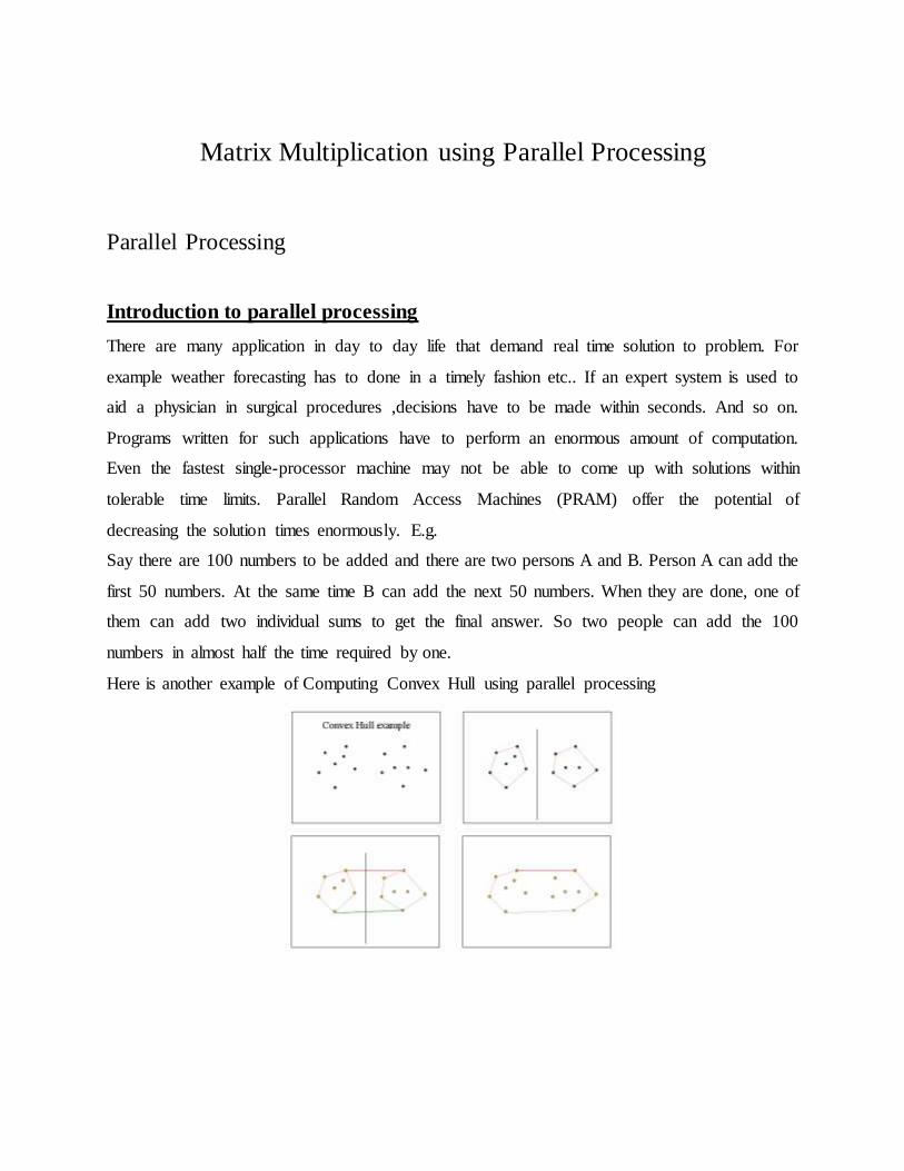
Here is another example of Computing Convex Hull using parallel processing

Take the set of points and divide the set into two halves Assume that recursive call computes the

convex hull of the two halves Conquer stage: take the two convex hulls and merge it to obtain

the convex hull for the entire set.

What is Computational Model

“A computational model is a mathematical model in computational science that requires

extensive computational resources to study the behavior of a complex system by computer

simulation.”

Random access machine model

Algorithms can be measured in a machine-independent way using the Random Access Machine

(RAM) model. This model assumes a single processor. In the RAM model, instructions are

executed one after the other, with no concurrent operations. This model of computation is an

abstraction that allows us to compare algorithms on the basis of performance. The assumptions

made in the RAM model to accomplish this are:

Each simple operation takes 1 time step.

Loops and subroutines are not simple operations.

Each memory access takes one time step, and there is no shortage of memory.

For any given problem the running time of algorithms is assumed to be the number of time steps.

The space used by an algorithm is assumed to be the number of RAM memory cells.

A model of computation whose memory consists of an unbounded sequence of registers, each of

which may hold an integer. In this model, arithmetic operations are allowed to compute the

address of a memory register.

In the RAM (Random Access Machine) we assume that any of the following operation can be

done in one unit of time: addition, subtraction, multiplication, division, comparison, memory

access, assignment, and so on. This model widely accepted as a valid sequential model.

An important feature of parallel computing that is absent in sequential computing is need for

interprocessor communication. For example given any problem, the processor have to

communicate among themselves and agree on the subproblems each will work on. Also they

need to communicate to see whether everyone has finished its task so on.

PRAM Model for Single Processor Machine. The designer of sequential algorithm typically formulates the algorithm using an abstract model

of computation called random access machine(RAM). In this model, the machine consist of a

single processor connected to a memory system. Each CPU include arithmetic operation, logical

operation, and memory access require one step access.

Standard Random Access Machine

Each Operation load, store, jump, add, etc takes one unit of time.

Simply general one model.

Basic model for sequential algorithm

Unbounded number of local memory cells

Each memory cell can hold an integer of unbounded size

Instruction set included –simple operations, data operations, comparator, branches

All operations take unit time

Time complexity = number of instructions executed

Space complexity = number of memory cells used

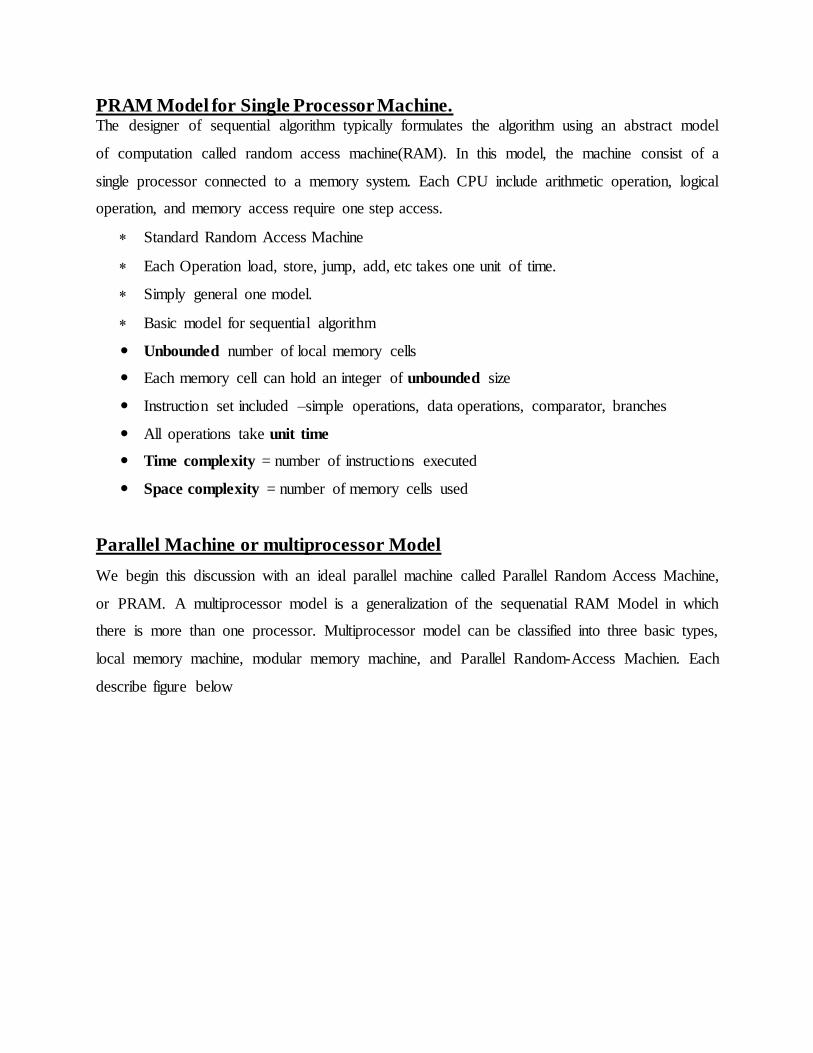
Parallel Machine or multiprocessor Model

We begin this discussion with an ideal parallel machine called Parallel Random Access Machine,

or PRAM. A multiprocessor model is a generalization of the sequenatial RAM Model in which

there is more than one processor. Multiprocessor model can be classified into three basic types,

local memory machine, modular memory machine, and Parallel Random-Access Machien. Each

describe figure below

“The Parallel Random Access Machine (PRAM) is an abstract model for parallel computation

which assumes that all the processors operate synchronously under a single clock and are able to

randomly access a large shared memory.”

A natural extension of the Random Access Machine(RAM), serial architecture is the

Parallel Random Access Machine, or PRAM

Pram Consist of p Processor and a global memory of unbounded size that is uniformly

accessible to all processors

Processors share a common clock but may execute different instruction in each cycle

PRAM Architecture

The parallel version of RAM constitutes an abstract model of the class of global-memory parallel

processors. The

abstraction consists of ignoring the details of the processor-to-memory interconnection network

and taking the view that each processor can access any memory location in each machine cycle,

independent of what other processors are doing.

Processor i can do the following in three phases of one cycle:

Fetch a value from address si in shared memory

Perform computations on data held in local registers

3. Store a value into address di in shared memory

Is an abstract machine for designing the algorithms applicable to parallel computers

Unbounded collection of RAM processors P0, P1, …,

Processors don’t have tape

Each processor has unbounded registers

Unbounded collection of share memory cells

All processors can access all memory cells in unit time

All communication via shared memory

Two or more processors may read simultaneously from the same cell

A write conflict occurs when two or more processors try to write simultaneously into

the same cell

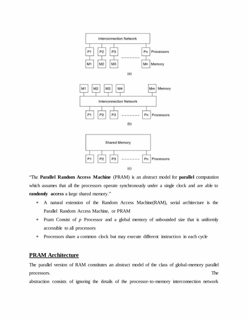
Classification of PRAM Model

The classification in is reminiscent of Flynn’s classification and offers yet another example of

the quest to invent four-letter abbreviations/acronyms in computer architecture! Note that here,

too, one of the categories is not very useful, because if concurrent writes are allowed, there is no

logical reason for excluding the less problematic concurrent reads. EREW PRAM is the most

realistic of the four submodels (to the extent that thousands of processors concurrently accessing

thousands of memory locations within a shared memory address space of millions or even

billions of locations can be considered realistic!). CRCW PRAM is the least restrictive

submodel, but has the disadvantage of requiring a conflict resolution mechanism to define the

effect of concurrent writes (more on this below). The default submodel, which is assumed when

nothing is said about the submodel, is CREW PRAM. For most computations, it is fairly easy to

organize the algorithm steps so that concurrent writes to the same location are never attempted.

CRCW PRAM is further classified according to how concurrent writes are handled. Here are a

few example submodels based on the semantics of concurrent writes in CRCW PRAM:

EREW Least “powerful”, most “realistic”

CREW Default

ERCW Not useful

CRCW Most “powerful”,

further subdivided

Reads from same location

Wri

tes t

o s

am

e lo

ca

tio

n

Exclusive

Co

ncurr

ent

Concurrent

Exclu

siv

e

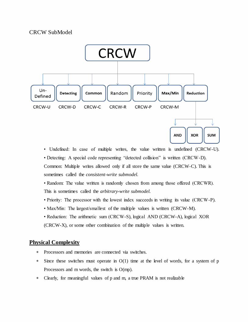
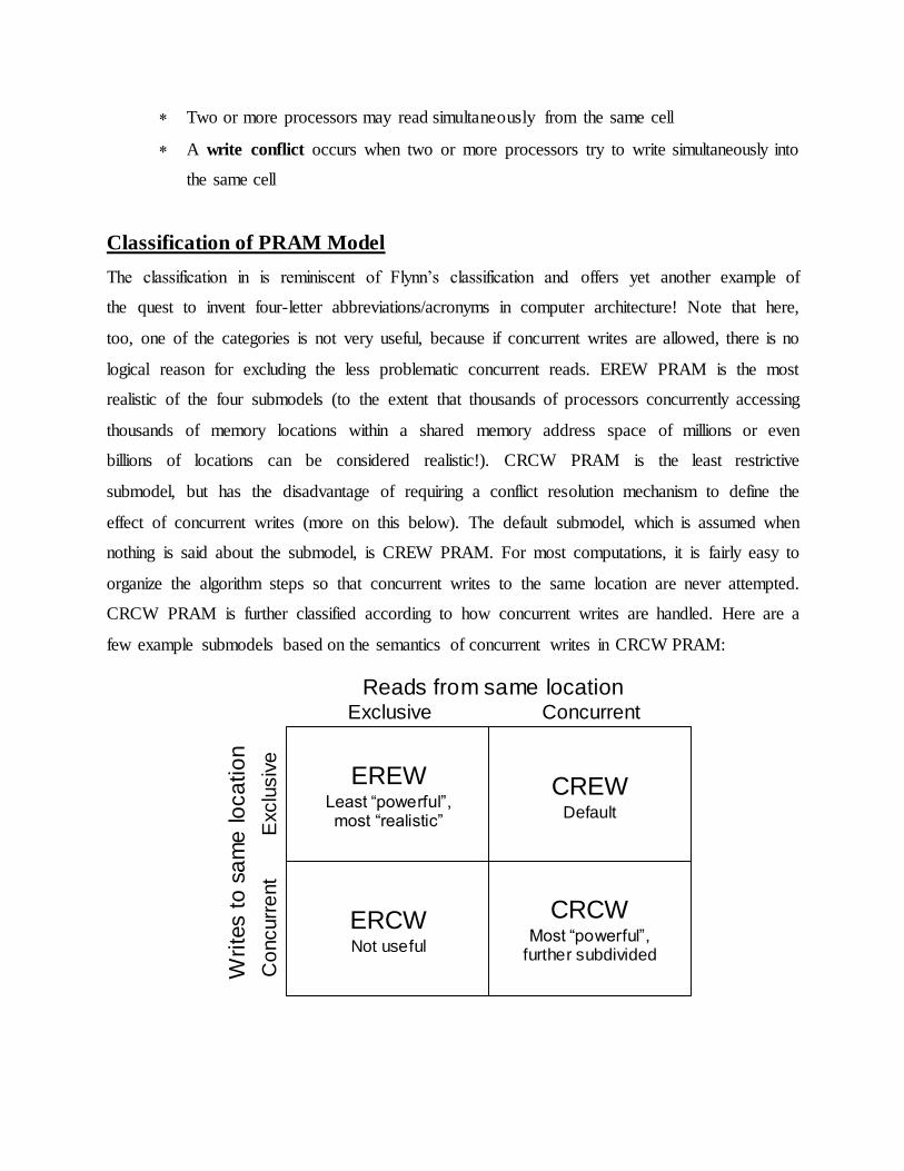
CRCW SubModel

• Undefined: In case of multiple writes, the value written is undefined (CRCW-U).

• Detecting: A special code representing “detected collision” is written (CRCW-D).

Common: Multiple writes allowed only if all store the same value (CRCW-C). This is

sometimes called the consistent-write submodel.

• Random: The value written is randomly chosen from among those offered (CRCWR).

This is sometimes called the arbitrary-write submodel.

• Priority: The processor with the lowest index succeeds in writing its value (CRCW-P).

• Max/Min: The largest/smallest of the multiple values is written (CRCW-M).

• Reduction: The arithmetic sum (CRCW-S), logical AND (CRCW-A), logical XOR

(CRCW-X), or some other combination of the multiple values is written.

Physical Complexity

Processors and memories are connected via switches.

Since these switches must operate in O(1) time at the level of words, for a system of p

Processors and m words, the switch is O(mp).

Clearly, for meaningful values of p and m, a true PRAM is not realizable

Relationship between different PRAM Submodel

The following relationships have been established between some of the PRAM submodels:

EREW < CREW < CRCW-D < CRCW-C < CRCW-R < CRCW-P

Even though all CRCW submodels are strictly more powerful than the EREW submodel, the

latter can simulate the most powerful CRCW submodel listed above with at most logarithmic

slowdown.

A p-processor CRCW-P (priority) PRAM can be simulated by a p-processor EREW PRAM with

a slowdown factor of Θ(log p). EREW PRAM to sort or find the smallest of p values in Θ(log p)

time, as we shall see later. To avoid concurrent writes, each processor writes an ID-address-value

triple into its corresponding element of a scratch list of size p, with the p processors then

cooperating to sort the list by the destination addresses, partition the list into segments

corresponding to common addresses (which are now adjacent in the sorted list), do a reduction

operation within each segment to remove all writes to the same location except the one with the

smallest processor ID, and finally write the surviving address-value pairs into memory. This final

write operation will clearly be of the exclusive variety.

Matrix Multiplication

Introduction to Matrix Multiplication.

We will show how to implement matrix multiplication C=C+A*B on several of the

communication networks discussed in the last lecture, and develop performance models to

predict how long they take. We will see that the performance depends on several factors.

we discuss PRAM matrix multiplication algorithms as representative examples of the class of

numerical problems. Matrix multiplication is quite important in its own right and is also used as

a building block in many other parallel algorithms. For example, matrix multiplication is useful

in solving graph problems when the graphs are represented by their adjacency or weight

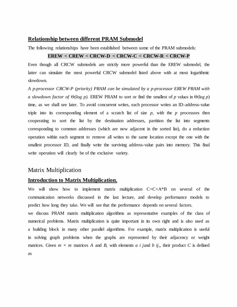
matrices. Given m × m matrices A and B, with elements a i jand b ij,, their product C is defined

as

The following O(m³)-step sequential algorithm can be used for multiplying m × m matrices:

Sequential matrix multiplication

for i = 0 to m – 1 do for j = 0 to m – 1 do

t := 0 for k = 0 to m – 1 do

t := t + aikbkj endfor cij := t

endfor endfor

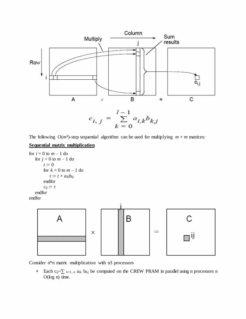
Consider n*n matric multiplication with n3 processors

Each cij=∑ k=1..n aik bkj be computed on the CREW PRAM in parallel using n processors n

O(log n) time.

On the EREW PRAM exclusive read of aij and bij values can be satisfied by making n

copies of a and b, which takes O(log n) time with n Processors

Total time is still O(log n)

Memory requirement is ofcourse much higher for the EREW PRAM

Complexity: Θ(n3)

Better Algorithm that improve slightly

Multiplication by block

PRAM matrix multiplication using m2 processors

Proc (i, j), 0 i, j < m, do begin

t := 0 for k = 0 to m – 1 do

t := t + aikbkj endfor cij := t

end

Because multiple processors will be reading the same row of A or the same column of B, the

above naive implementation of the algorithm would require the CREW submodel. However, it is

possible to convert the algorithm to an EREW PRAM algorithm by skewing the memory

accesses (how?).

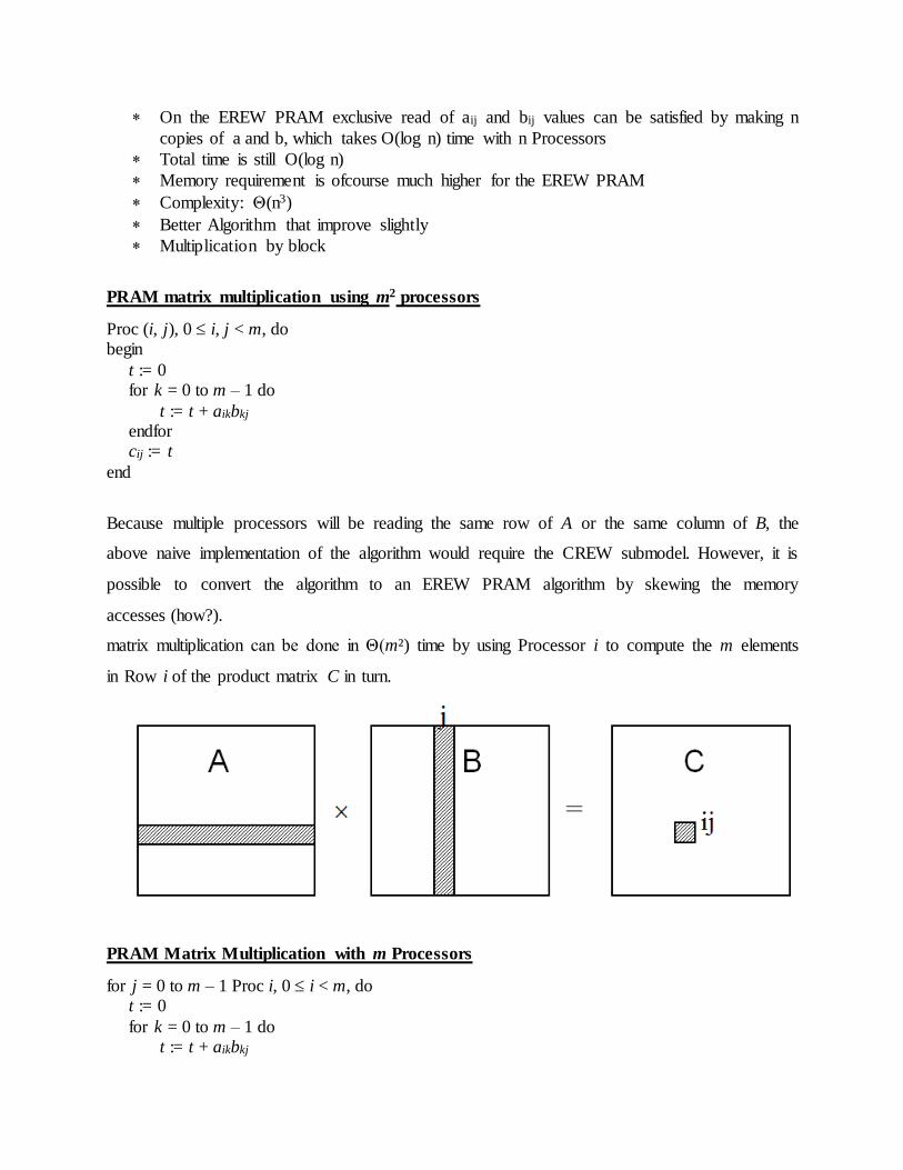
matrix multiplication can be done in Θ(m²) time by using Processor i to compute the m elements

in Row i of the product matrix C in turn.

PRAM Matrix Multiplication with m Processors

for j = 0 to m – 1 Proc i, 0 i < m, do t := 0

for k = 0 to m – 1 do t := t + aikbkj

endfor cij := t

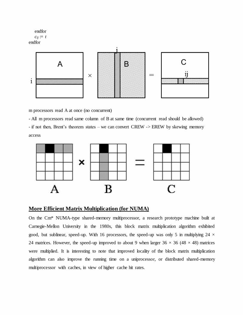
endfor

m processors read A at once (no concurrent)

- All m processors read same column of B at same time (concurrent read should be allowed)

- if not then, Brent’s theorem states – we can convert CREW -> EREW by skewing memory

access

More Efficient Matrix Multiplication (for NUMA)

On the Cm* NUMA-type shared-memory multiprocessor, a research prototype machine built at

Carnegie-Mellon University in the 1980s, this block matrix multiplication algorithm exhibited

good, but sublinear, speed-up. With 16 processors, the speed-up was only 5 in multiplying 24 ×

24 matrices. However, the speed-up improved to about 9 when larger 36 × 36 (48 × 48) matrices

were multiplied. It is interesting to note that improved locality of the block matrix multiplication

algorithm can also improve the running time on a uniprocessor, or distributed shared-memory

multiprocessor with caches, in view of higher cache hit rates.

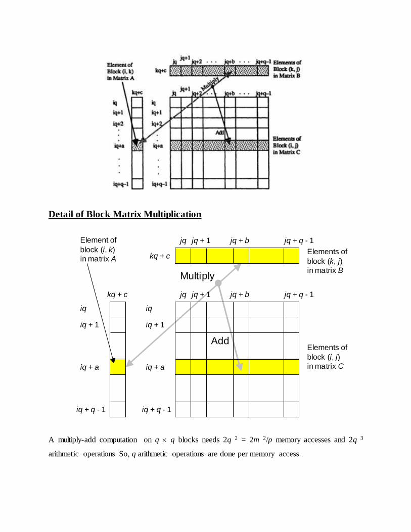
Detail of Block Matrix Multiplication

A multiply-add computation on q q blocks needs 2q 2 = 2m 2/p memory accesses and 2q 3

arithmetic operations So, q arithmetic operations are done per memory access.

iq + q - 1

iq + a

iq + 1

iq

jq jq + b jq + q - 1

kq + c

kq + c

iq + q - 1

iq + a

iq + 1

iq

jq jq + 1 jq + b jq + q - 1

Multiply

Add Elements of

block (i, j)

in matrix C

Elements of

block (k, j)

in matrix B

Element of

block (i, k)

in matrix A

jq + 1

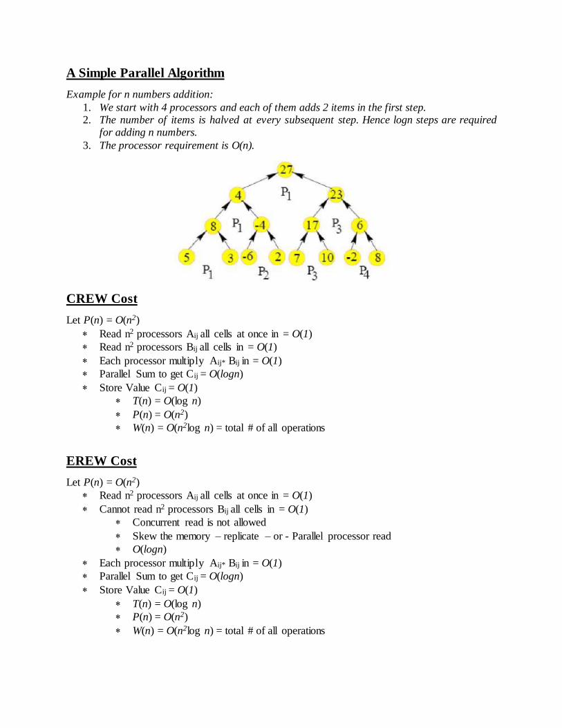
A Simple Parallel Algorithm

Example for n numbers addition:

1. We start with 4 processors and each of them adds 2 items in the first step. 2. The number of items is halved at every subsequent step. Hence logn steps are required

for adding n numbers.

3. The processor requirement is O(n).

CREW Cost

Let P(n) = O(n2)

Read n2 processors Aij all cells at once in = O(1)

Read n2 processors Bij all cells in = O(1)

Each processor multiply Aij* Bij in = O(1)

Parallel Sum to get Cij = O(logn)

Store Value Cij = O(1)

T(n) = O(log n)

P(n) = O(n2)

W(n) = O(n2log n) = total # of all operations

EREW Cost

Let P(n) = O(n2)

Read n2 processors Aij all cells at once in = O(1)

Cannot read n2 processors Bij all cells in = O(1)

Concurrent read is not allowed

Skew the memory – replicate – or - Parallel processor read

O(logn)

Each processor multiply Aij* Bij in = O(1)

Parallel Sum to get Cij = O(logn)

Store Value Cij = O(1)

T(n) = O(log n)

P(n) = O(n2)

W(n) = O(n2log n) = total # of all operations

Advantages of PRAM Model

PRAM removes algorithmic details concerning synchronization and communicating,

allowing the algorithm designer to focus on problem properties

A PRAM algorithm includes an explicit understanding of the operation performed at each

time unit and an explicit allocation of processors to jobs at each time unit.

PRAM designer paradigm have turned out to be robust and have been mapped efficiently

onto many other parallel models and even network models

Disadvantage of PRAM Model

Model Inaccuracies unbounded local memory(register)

All operation takes unit time processors run in lock steps

Unaccounted costs Non-local memory access

Latency Bandwidth Memory Access Contention

Conclusion

PRAM algorithm is the source of most fundamental ideas

It’s a source of inspiration for algorithms

PRAM is simple and easy to understand.

The improved locality of block matrix multiplication can also improve the running time on a uniprocessor, or distributed shared-memory multiprocessor with caches.

Reason: Higher Cache Higher Hit Rates