Statistics 1 Discrete Random Variables Section 2

1

DISCRETE RANDOM VARIABLES

Section 2

Choose from the following:

Introduction: Car share scheme a success

Example 4.3: A discrete random variable

Example 4.4: Laura’s Milk Bill

End presentation

Statistics 1 Discrete Random Variables Section 2

2

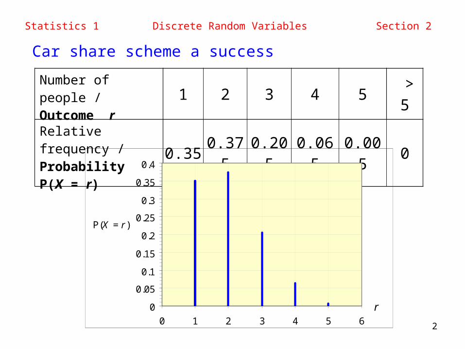
Car share scheme a success

Number of people / Outcome r 1 2 3 4 5 > 5

Relative frequency / Probability P(X = r) 0.35 0.375 0.205 0.065 0.005 0

0

0.05

0.1

0.15

0.2

0.25

0.3

0.35

0.4

0 1 2 3 4 5 6

r

P(X = r )

Statistics 1 Discrete Random Variables Section 2

3

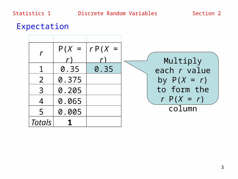
Expectation

r P(X = r) r P(X = r)1 0.35 0.352 0.3753 0.2054 0.0655 0.005

Totals 1

Multiply each r value by P(X = r)

to form ther P(X = r)column

Statistics 1 Discrete Random Variables Section 2

4

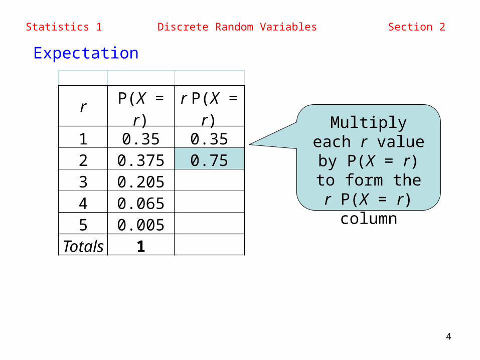
Expectation

r P(X = r) r P(X = r)1 0.35 0.352 0.375 0.753 0.2054 0.0655 0.005

Totals 1

Multiply each r value by P(X = r)

to form ther P(X = r)column

Statistics 1 Discrete Random Variables Section 2

5

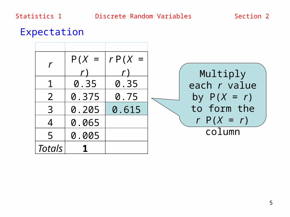
Expectation

r P(X = r) r P(X = r)1 0.35 0.352 0.375 0.753 0.205 0.6154 0.0655 0.005

Totals 1

Multiply each r value by P(X = r)

to form ther P(X = r)column

Statistics 1 Discrete Random Variables Section 2

6

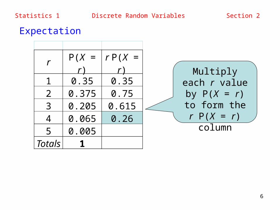
Expectation

r P(X = r) r P(X = r)1 0.35 0.352 0.375 0.753 0.205 0.6154 0.065 0.265 0.005

Totals 1

Multiply each r value by P(X = r)

to form ther P(X = r)column

Statistics 1 Discrete Random Variables Section 2

7

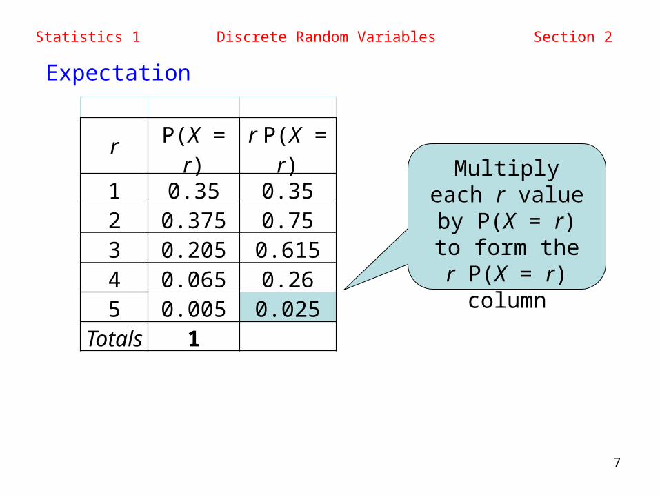
Expectation

r P(X = r) r P(X = r)1 0.35 0.352 0.375 0.753 0.205 0.6154 0.065 0.265 0.005 0.025

Totals 1

Multiply each r value by P(X = r)

to form ther P(X = r)column

Statistics 1 Discrete Random Variables Section 2

8

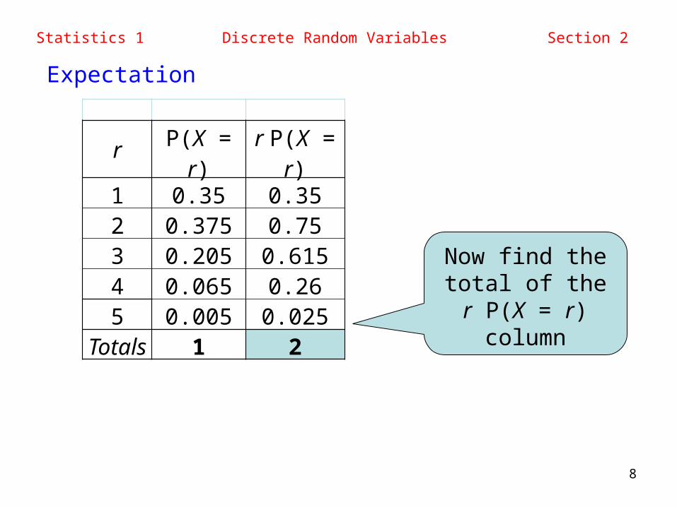
Expectation

r P(X = r) r P(X = r)1 0.35 0.352 0.375 0.753 0.205 0.6154 0.065 0.265 0.005 0.025

Totals 1 2

Now find the total of the

r P(X = r)column

Statistics 1 Discrete Random Variables Section 2

9

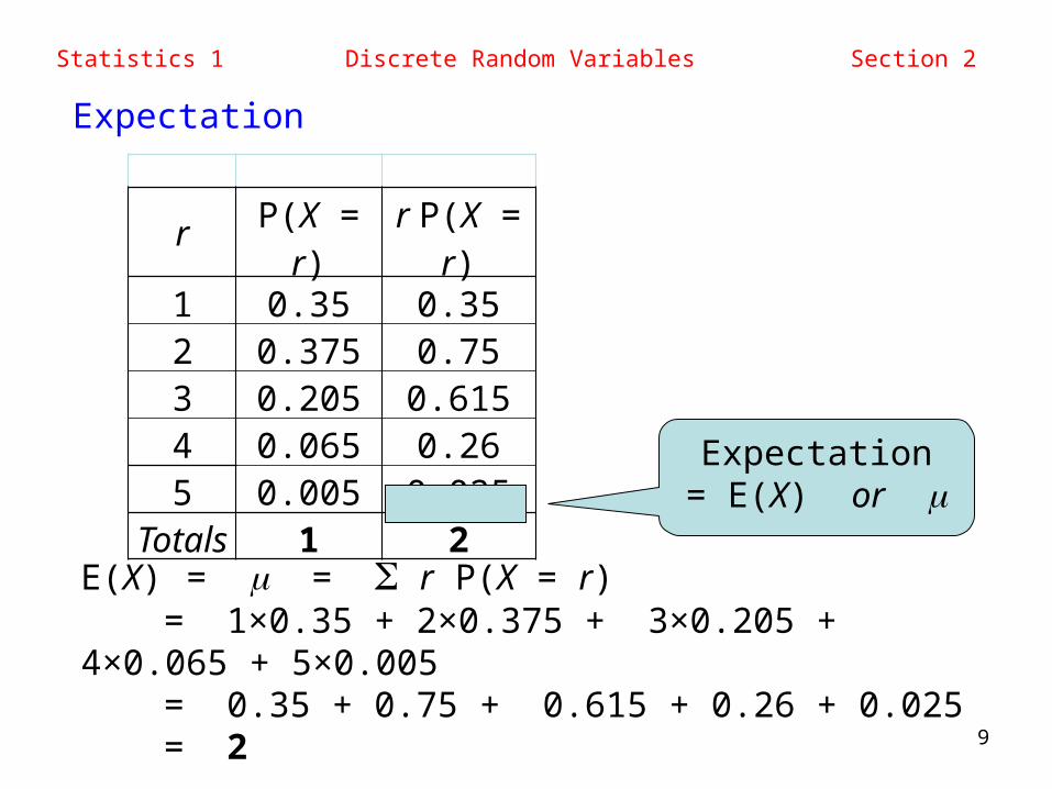
Expectation

E(X) = m = S r P(X = r)= 1×0.35 + 2×0.375 + 3×0.205 + 4×0.065 + 5×0.005 = 0.35 + 0.75 + 0.615 + 0.26 + 0.025 = 2

r P(X = r) r P(X = r)1 0.35 0.352 0.375 0.753 0.205 0.6154 0.065 0.265 0.005 0.025

Totals 1 2

Expectation= E(X) or m

Statistics 1 Discrete Random Variables Section 2

10

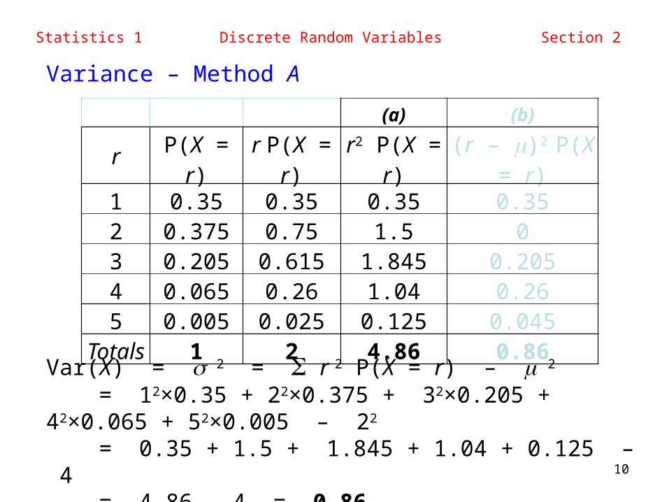
Var(X) = s 2 = S r 2 P(X = r) – m 2 = 12×0.35 + 22×0.375 + 32×0.205 + 42×0.065 + 52×0.005 – 22

= 0.35 + 1.5 + 1.845 + 1.04 + 0.125 – 4= 4.86 – 4 = 0.86

Variance – Method A

(a) (b)

r P(X = r) r P(X = r) r2 P(X = r) (r – m)2 P(X = r)

1 0.35 0.35 0.35 0.352 0.375 0.75 1.5 03 0.205 0.615 1.845 0.2054 0.065 0.26 1.04 0.265 0.005 0.025 0.125 0.045

Totals 1 2 4.86 0.86

Statistics 1 Discrete Random Variables Section 2

11

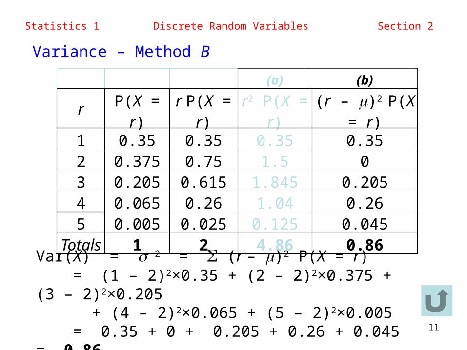
Variance – Method B

(a) (b)

r P(X = r) r P(X = r) r2 P(X = r) (r – m)2 P(X = r)

1 0.35 0.35 0.35 0.352 0.375 0.75 1.5 03 0.205 0.615 1.845 0.2054 0.065 0.26 1.04 0.265 0.005 0.025 0.125 0.045

Totals 1 2 4.86 0.86Var(X) = s 2 = S (r – m)2 P(X = r)

= (1 – 2)2×0.35 + (2 – 2)2×0.375 + (3 – 2)2×0.205 + (4 – 2)2×0.065 + (5 – 2)2×0.005

= 0.35 + 0 + 0.205 + 0.26 + 0.045 = 0.86

Statistics 1 Discrete Random Variables Section 2

12

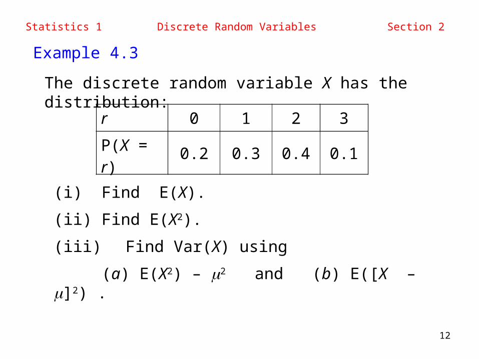
Example 4.3

The discrete random variable X has the distribution:

(i) Find E(X).

(ii) Find E(X2).

(iii) Find Var(X) using

(a) E(X2) – m2 and (b) E([X – m]2) .

r 0 1 2 3

P(X = r) 0.2 0.3 0.4 0.1

Statistics 1 Discrete Random Variables Section 2

13

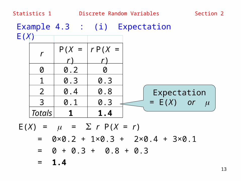
Example 4.3 : (i) Expectation E(X)

r P(X = r) r P(X = r)0 0.2 01 0.3 0.32 0.4 0.83 0.1 0.3

Totals 1 1.4

Expectation= E(X) or m

E(X) = m = S r P(X = r)

= 0×0.2 + 1×0.3 + 2×0.4 + 3×0.1

= 0 + 0.3 + 0.8 + 0.3

= 1.4

Statistics 1 Discrete Random Variables Section 2

14

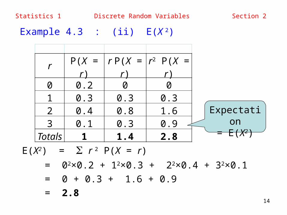
Example 4.3 : (ii) E(X 2)

r P(X = r) r P(X = r) r2 P(X = r)0 0.2 0 01 0.3 0.3 0.32 0.4 0.8 1.63 0.1 0.3 0.9

Totals 1 1.4 2.8

E(X2) = S r 2 P(X = r)

= 02×0.2 + 12×0.3 + 22×0.4 + 32×0.1

= 0 + 0.3 + 1.6 + 0.9

= 2.8

Expectation= E(X2)

Statistics 1 Discrete Random Variables Section 2

15

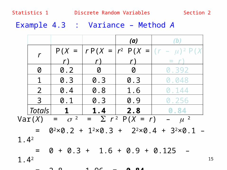
Example 4.3 : Variance – Method A

(a) (b)

r P(X = r) r P(X = r) r2 P(X = r) (r – m)2 P(X = r)

0 0.2 0 0 0.3921 0.3 0.3 0.3 0.0482 0.4 0.8 1.6 0.1443 0.1 0.3 0.9 0.256

Totals 1 1.4 2.8 0.84Var(X) = s 2 = S r 2 P(X = r) – m 2

= 02×0.2 + 12×0.3 + 22×0.4 + 32×0.1 – 1.42

= 0 + 0.3 + 1.6 + 0.9 + 0.125 – 1.42

= 2.8 – 1.96 = 0.84

Statistics 1 Discrete Random Variables Section 2

16

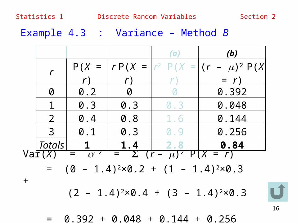
Example 4.3 : Variance – Method B

(a) (b)

r P(X = r) r P(X = r) r2 P(X = r) (r – m)2 P(X = r)

0 0.2 0 0 0.3921 0.3 0.3 0.3 0.0482 0.4 0.8 1.6 0.1443 0.1 0.3 0.9 0.256

Totals 1 1.4 2.8 0.84Var(X) = s 2 = S (r – m)2 P(X = r)

= (0 – 1.4)2×0.2 + (1 – 1.4)2×0.3 + (2 – 1.4)2×0.4 + (3 – 1.4)2×0.3

= 0.392 + 0.048 + 0.144 + 0.256 = 0.84

Statistics 1 Discrete Random Variables Section 2

17

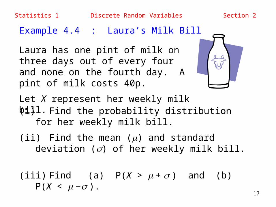
Example 4.4 : Laura’s Milk Bill

Laura has one pint of milk on three days out of every four and none on the fourth day. A pint of milk costs 40p.

Let X represent her weekly milk bill.

(i) Find the probability distribution for her weekly milk bill.

(ii) Find the mean (m) and standard deviation (s) of her weekly milk bill.

(iii) Find (a) P(X > m + s ) and (b) P(X < m −s ).

Statistics 1 Discrete Random Variables Section 2

18

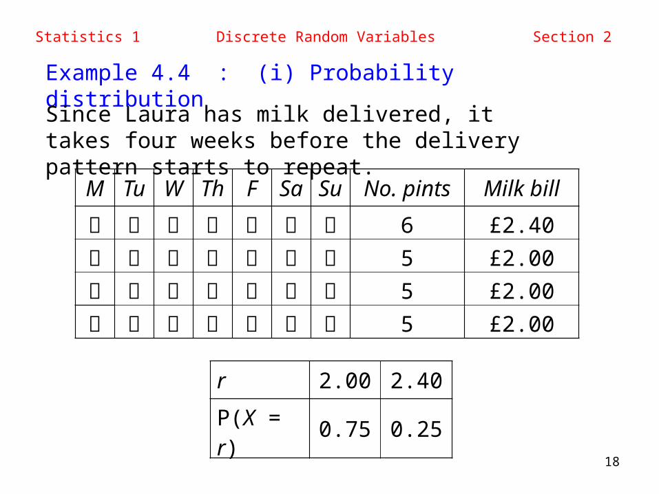
Example 4.4 : (i) Probability distribution

Since Laura has milk delivered, it takes four weeks before the delivery pattern starts to repeat.

M Tu W Th F Sa Su No. pints Milk bill

6 £2.40

5 £2.00

5 £2.00

5 £2.00

r 2.00 2.40

P(X = r) 0.75 0.25

Statistics 1 Discrete Random Variables Section 2

19

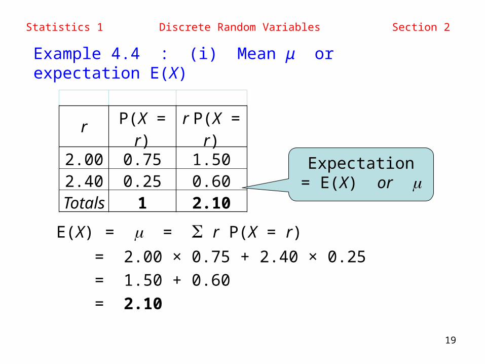
Example 4.4 : (i) Mean μ or expectation E(X)

r P(X = r) r P(X = r)2.00 0.75 1.502.40 0.25 0.60

Totals 1 2.10

Expectation= E(X) or m

E(X) = m = S r P(X = r)

= 2.00 × 0.75 + 2.40 × 0.25

= 1.50 + 0.60

= 2.10

Statistics 1 Discrete Random Variables Section 2

20

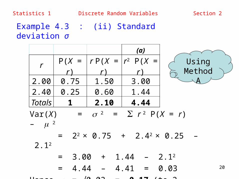
Example 4.3 : (ii) Standard deviation σ

(a)

r P(X = r) r P(X = r) r2 P(X = r)2.00 0.75 1.50 3.002.40 0.25 0.60 1.44

Totals 1 2.10 4.44

Var(X) = s 2 = S r 2 P(X = r) – m 2

= 22 × 0.75 + 2.42 × 0.25 – 2.12

= 3.00 + 1.44 – 2.12

= 4.44 – 4.41 = 0.03

Hence s = √0.03 = 0.17 (to 2 d.p.)

Using Method A

Statistics 1 Discrete Random Variables Section 2

21

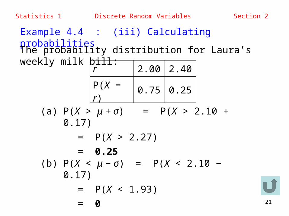
Example 4.4 : (iii) Calculating probabilities

r 2.00 2.40

P(X = r) 0.75 0.25

The probability distribution for Laura’s weekly milk bill:

(a) P(X > μ + σ) = P(X > 2.10 + 0.17)

= P(X > 2.27)

= 0.25

(b) P(X < μ − σ) = P(X < 2.10 − 0.17)

= P(X < 1.93)

= 0