Biosight: Quantitative Methods for Policy Analysis - Introduction to GAMS, Linear Programming

Day 1: Introduction to GAMS, Linear Programming, and PMP

Day 1 NotesHowitt and Msangi 1

Understand basic GAMS syntax

Calibrate and run regional or farm models from minimal datasets

Calculate regional water demands

Calculate elasticity of water demand

Estimate the value of rural water demand for water policy


Linear Models

Linear Programming: Primal

Positive Mathematical Programming



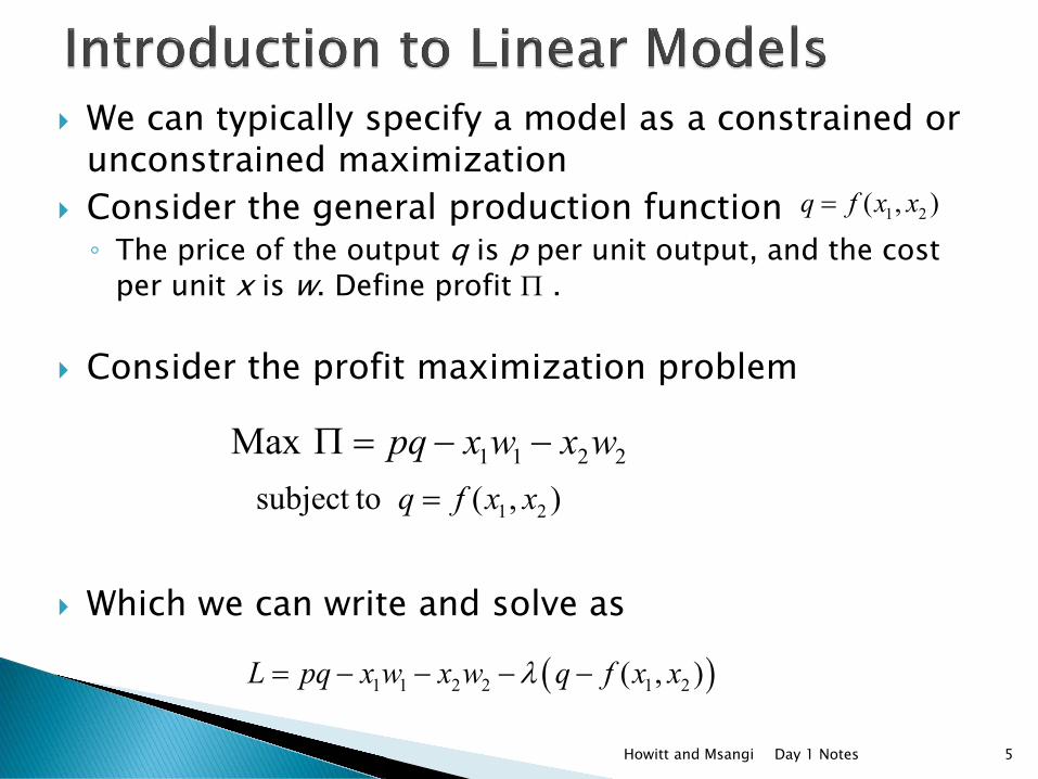
We can typically specify a model as a constrained or unconstrained maximization

Consider the general production function ◦ The price of the output q is p per unit output, and the cost

per unit x is w. Define profit Π .

Consider the profit maximization problem

Which we can write and solve as


1 2( , )q f x x=

1 1 2 2Max pq x w x wΠ = − −

1 2subject to ( , )q f x x=

( )1 1 2 2 1 2( , )L pq x w x w q f x xλ= − − − −

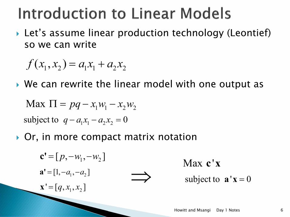
Let’s assume linear production technology (Leontief) so we can write

We can rewrite the linear model with one output as

Or, in more compact matrix notation


1 2 1 1 2 2( , )f x x a x a x= +

1 1 2 2Max pq x w x wΠ = − −

1 1 2 2subject to 0q a x a x− − =

1 2[ , , ]p w w= − −c'

1 2[1, , ]a a= − −a'

1 2' [ , , ]q x x=x

Max 'c xsubject to ' 0=a x⇒

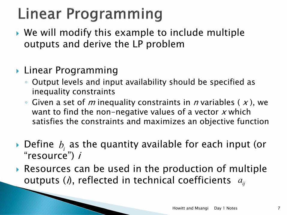
We will modify this example to include multiple outputs and derive the LP problem

Linear Programming◦ Output levels and input availability should be specified as

inequality constraints◦ Given a set of m inequality constraints in n variables ( x ), we

want to find the non-negative values of a vector x which satisfies the constraints and maximizes an objective function

Define as the quantity available for each input (or “resource”) i

Resources can be used in the production of multiple outputs (i), reflected in technical coefficients


ib

ija

Let’s define the matrix of technical coefficients and vector of available inputs

And we can write the general LP as

Note that we have 2 (constrained) inputs and 2 outputs in our example, but this notation generalizes to any number.


11 12

21 22

a aa a

=

A1

2

bb

=

b

Max 'c xsubject to ≤Ax b

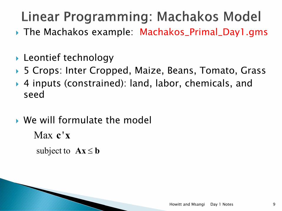
The Machakos example: Machakos_Primal_Day1.gms

Leontief technology 5 Crops: Inter Cropped, Maize, Beans, Tomato, Grass 4 inputs (constrained): land, labor, chemicals, and

seed

We will formulate the model


Max 'c xsubject to ≤Ax b


[ ]1 2 3 4 5' [ ]x x x x x Inter Cropped Maize Beans Tomato Grass= = −x

1

2

3

4

Land (hectares) 2.78Labor (person days) 250

Chemicals (kg) 6,000Seed (kg) 6,000

bbbb

= ≡ =

b

11 12 13 14 15

21 22 23 24 25

31 32 33 34 35

41 42 43 44 45

1 1 1 1 140.3 159 126.5 136 08.75 83.9 12.03 181.3 3043 44.6 50.3 22 0

a a a a aa a a a aa a a a aa a a a a

= =

A

[ ]1 2 3 4 5' [ ] 13,563 8,350 31,125 37,704 24,980c c c c c= =c

Let’s multiply out a constraint and interpret

Constraint 3:

Interpretation: total use of chemicals in the production of all crops must be less than or equal to the total available chemicals

Numerically:

We will formulate and solve the model during the afternoon session


31 1 32 2 33 3 34 4 35 5 3a x a x a x a x a x b+ + + + ≤

1 2 3 4 58.75 83.9 12.03 181.3 30 6,000x x x x x kg+ + + + ≤

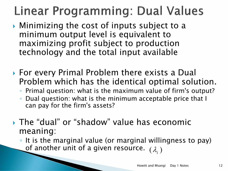
Minimizing the cost of inputs subject to a minimum output level is equivalent to maximizing profit subject to production technology and the total input available

For every Primal Problem there exists a Dual Problem which has the identical optimal solution. ◦ Primal question: what is the maximum value of firm's output?◦ Dual question: what is the minimum acceptable price that I

can pay for the firm's assets?

The “dual” or “shadow” value has economic meaning:◦ It is the marginal value (or marginal willingness to pay)

of another unit of a given resource.


( )iλ

Dual objective function◦ Equal to the sum of the imputed values of the total resource

stock of the firm (amount of money that you would have to offer a firm owner for a buy-out).

Dual Constraints◦ Set of prices for the fixed resources (or assets) of the firm that

would yield at least an equivalent return to the owner as producing a vector of products ( x ), which can be sold for prices ( c ), from these resources.

Where do these values come from?


Max 'c xsubject to ( )≤Ax b λ


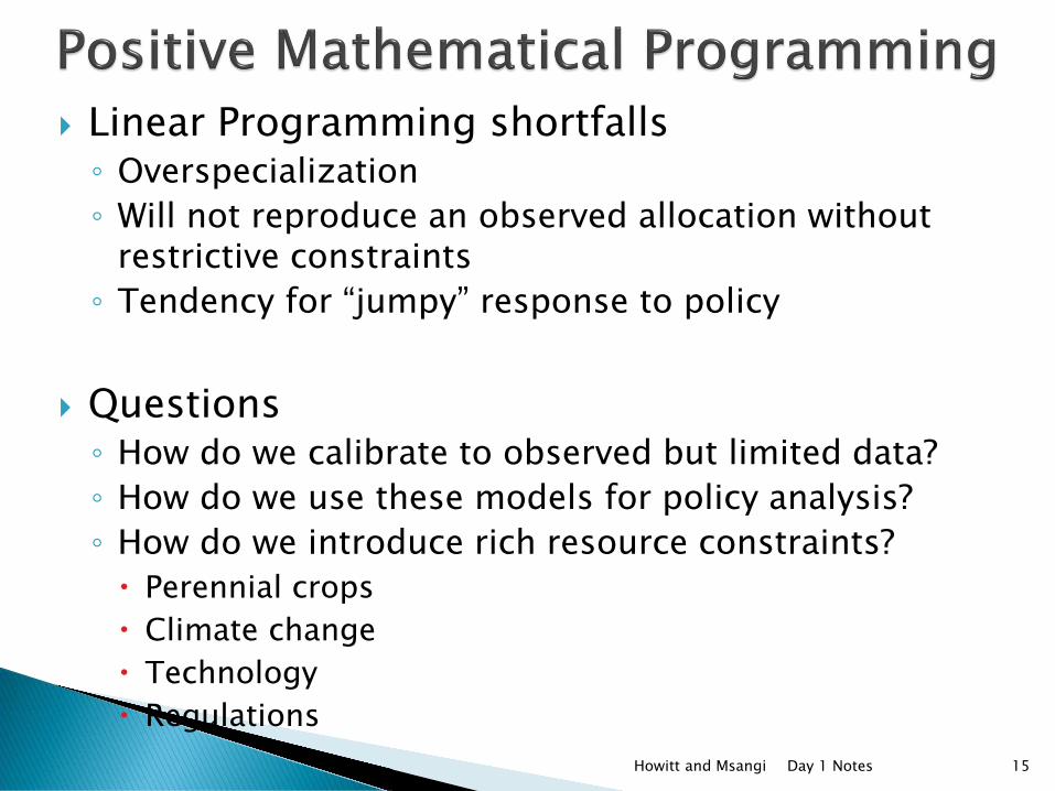
Linear Programming shortfalls◦ Overspecialization ◦ Will not reproduce an observed allocation without

restrictive constraints◦ Tendency for “jumpy” response to policy

Questions◦ How do we calibrate to observed but limited data?◦ How do we use these models for policy analysis?◦ How do we introduce rich resource constraints? Perennial crops Climate change Technology Regulations


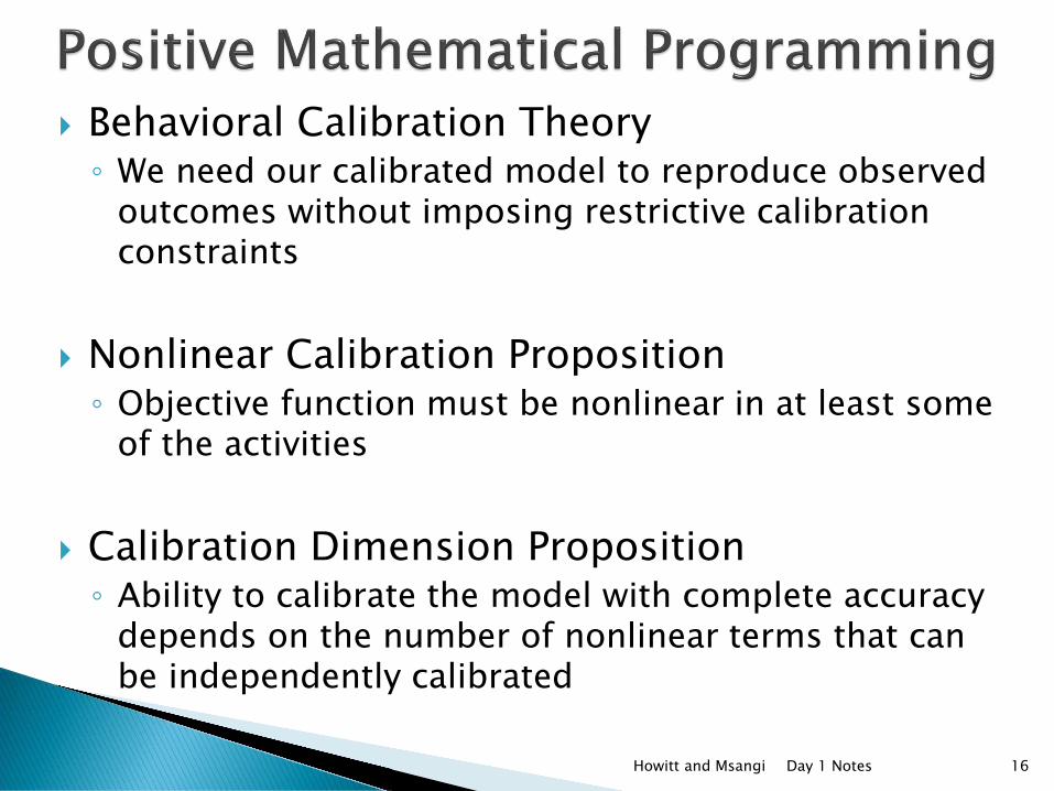
Behavioral Calibration Theory◦ We need our calibrated model to reproduce observed

outcomes without imposing restrictive calibration constraints

Nonlinear Calibration Proposition◦ Objective function must be nonlinear in at least some

of the activities

Calibration Dimension Proposition◦ Ability to calibrate the model with complete accuracy

depends on the number of nonlinear terms that can be independently calibrated


Let marginal revenue = KSh 500/hectare Average cost = KSh 300/hectare Observed acreage allocation = 50 hectares

Introduce calibration constraint to estimate residual cost needed to calibrate crop acreage to 50


Max 500 300x x−

subject to 50x ≤

2λ

We need to introduce a nonlinear term in the objective function to achieve calibration. Here we introduce a quadratic total cost function. This is a common approach in PMP.

Under unconstrained optimization, MR=MC◦ For this condition to hold at x*=50 it must be that is the

difference at the constrained calibration value (MR-AC).◦ We know that MR=MC◦ Therefore , since we require MR=MC at x*=50


20.5TC x xα γ= +

2λ

2 MC - ACλ =

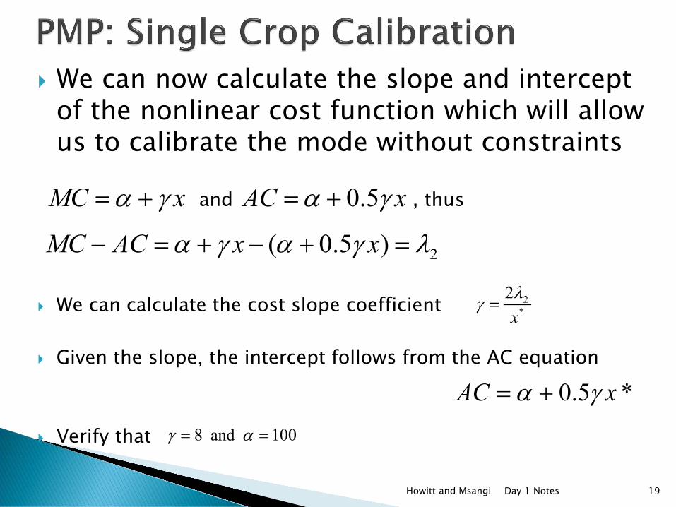
We can now calculate the slope and intercept of the nonlinear cost function which will allow us to calibrate the mode without constraints

and , thus

We can calculate the cost slope coefficient

Given the slope, the intercept follows from the AC equation

Verify that


MC xα γ= + 0.5AC xα γ= +

2( 0.5 )MC AC x xα γ α γ λ− = + − + =

2*

2xλγ =

0.5 *AC xα γ= +

8 and 100γ α= =

Combine this information and introduce the calibrated cost function into an unconstrained problem

Verify that we get the observed allocation as the optimal solution through standard unconstrained maximization◦ We see that x=50, which is our observed allocation and we have verified that

the model calibrates


2500 0.5Max x x xα γΠ = − −2500 100 0.5(8)Max x x xΠ = − −

2400 4Max x xΠ = −

Now the model can be used for policy simulations

The unconstrained profit maximization problem reproduces the observed base year

We can introduce changes and evaluate the response without restrictive calibration constraints

The method extends to multiple crops


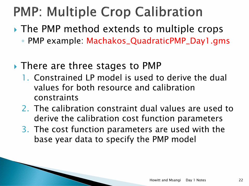
The PMP method extends to multiple crops◦ PMP example: Machakos_QuadraticPMP_Day1.gms

There are three stages to PMP1. Constrained LP model is used to derive the dual

values for both resource and calibration constraints

2. The calibration constraint dual values are used to derive the calibration cost function parameters

3. The cost function parameters are used with the base year data to specify the PMP model


2 Crop example: wheat and oats Observed Data: 2 ha oats and 3 ha wheat

(total farm size of 5 hectares)


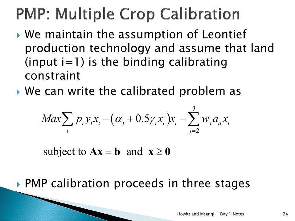
We maintain the assumption of Leontief production technology and assume that land (input i=1) is the binding calibrating constraint

We can write the calibrated problem as

PMP calibration proceeds in three stages


( )3

20.5i i i i i i i j ij i

i jMax p y x x x w a xα γ

=

− + −∑ ∑

subject to and = ≥Ax b x 0

Stage 1 Formulate and solve the constrained LP and

note the dual values () We introduce a perturbation term to decouple

resource and calibration constraints


2

1

1

max ( ) ( )

5 ( )3 ( )2 ( )

w w w w o o o o

w o

w w

o o

y p w x y p w xsubject tox xxx

λε λε λ

Π = − + −

+ ≤≤ +≤ +

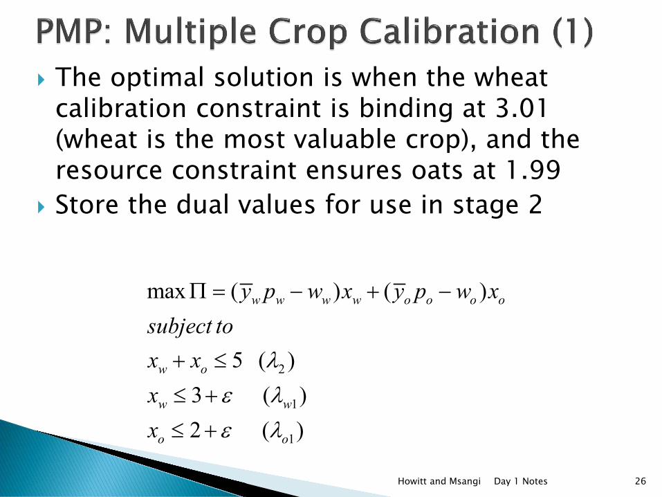
The optimal solution is when the wheat calibration constraint is binding at 3.01 (wheat is the most valuable crop), and the resource constraint ensures oats at 1.99

Store the dual values for use in stage 2


2

1

1

max ( ) ( )

5 ( )3 ( )2 ( )

w w w w o o o o

w o

w w

o o

y p w x y p w xsubject tox xxx

λε λε λ

Π = − + −

+ ≤≤ +≤ +

Stage 2 Derive the parameters of the quadratic total

cost function◦ Use same logic as in the single crop example

Notice two types of crops in the problem depending on which constraint is binding◦ Calibrated crops◦ Marginal crops

Calculate the cost intercept and slope for the calibrated wheat crop


Graphically


Stage 3 No restrictive calibration constraints

Calibration checks◦ Hectare allocation (all input allocation)◦ Input cost = Value Marginal Product

Can use the model for policy simulation


( )3

20.5 ,i i i i i i i j ij i

i jMax p y x x x w a x where i o wα γ

=

− + − =∑ ∑

0 5wx x+ ≤

We have covered a range of topics◦ Linear models◦ Linear Programming Primal Dual

◦ Positive Mathematical Programming Single crop mathematical derivation Multiple crop generalization

This afternoon we will revisit these topics in GAMS◦ Intro.gms◦ Machakos_Primal_Day1.gms◦ Machakos_Dual_Day1.gms◦ Machakos_QuadraticPMP_Day1.gms


Education

Biosight: Quantitative Methods for Policy Analysis - Introduction to GAMS, Linear Programming