Embed Size (px)
Citation preview

WORKING PAPERS
Social Centipedes: the Impact of Group Identity on Preferences and Reasoning
Chloé Le Coq
James Tremewan Alexander K. Wagner
August 2013
Working Paper No: 1305
DEPARTMENT OF ECONOMICS
UNIVERSITY OF VIENNA
All our working papers are available at: http://mailbox.univie.ac.at/papers.econ
Social Centipedes: the Impact of Group
Identity on Preferences and Reasoning∗
Chloe Le Coq† James Tremewan‡ Alexander K. Wagner§
This version September 12, 2013
Abstract
Using a group identity manipulation we examine the role of social preferences in
an experimental one-shot centipede game. Contrary to what social preference theory
would predict, we find that players continue longer when playing with outgroup
members. Our explanation rests on two observations: (i) players should only stop
if they are sufficiently confident that their partner will stop at the next node, given
the exponentially-increasing payoffs in the game, and (ii) players are more likely
to have this degree of certainty if they are matched with someone from the same
group, whom they view as similar to themselves and thus predictable. We find
strong statistical support for this argument. We conclude that group identity not
only impacts a player’s utility function, as identified in earlier research, but also
affects her reasoning about the partner’s behavior.
Keywords: Group identity, centipede game, prospective reference theory
JEL-Classification: C72, C91, C92, D83
∗We are grateful to Carlos Alos-Ferrer, Tore Ellingsen, Guido Friebel, Lorenz Gotte, Charles Holt,
Magnus Johannesson, Toshiji Kawagoe, Michael Kosfeld, Rachel E. Kranton, Hirokazu Takizawa, Marie
Claire Villeval and Irenaeus Wolff for helpful discussions and comments. In particular we thank Yan
Chen and Sherry Li for providing us with the original z-tree code used in Chen and Li (2009). We also
thank seminar participants at the University of Canterbury, University of Cologne, University of Frankfurt,
University of Geneva, University of Heidelberg, University of Munich, Stockholm School of Economics, as
well as conference participants at the IMEBE in Castellon, the THEEM in Kreuzlingen, the UECE Meeting
in Lisbon, the 4th World Congress of the Game Theory Society in Istanbul, and the BABEE Workshop
in San Francisco for useful comments. An earlier version of this paper was titled “Social preferences and
bounded rationality in the centipede game”.†SITE, Stockholm School of Economics (Sweden), Email: [email protected]‡Department of Economics, University of Vienna (Austria), Email: [email protected]§Department of Economics, University of Cologne (Germany), Email: [email protected]
1
1 Introduction
The centipede game, first introduced by Rosenthal (1981), has attracted much attention
both in the theoretical and experimental game theory literature. Many variations of this
game have been explored, but all share the same basic structure. Two players alternate in
their decision to continue or terminate the game. Payoffs are such that if a player chooses
to continue while her partner stops at the subsequent node, she receives less than if she
decides to stop immediately. Under common knowledge of rationality (Aumann, 1995,
1998), backward induction leads to the unique subgame-perfect Nash equilibrium where
players choose to stop at each of their decision nodes, the game thus ending at the first
node.
It has been repeatedly demonstrated in experimental studies, however, that the game
is rarely terminated at the first node. Most of the literature has argued that the system-
atic deviations from the subgame-perfect equilibrium outcome result from some form of
bounded rationality.1 With the exception of McKelvey and Palfrey (1992) and Fey et al.
(1996), who allow for altruistic behavior, none of the papers has explicitly tested for the
possible import of social preferences in the centipede game.
Our experiment was designed to examine the impact of social preferences on behav-
ior in the centipede game. As in Chen and Li (2009), participants are assigned to near
“minimal” groups according to their preferences over paintings and interact with ingroup
or outgroup members. It is well established that group identity manipulations increase
altruism, positive reciprocity and the desire for maximizing social welfare among ingroup
partners (for an overview, see Chen and Li, 2009; Chen and Chen, 2011; Goette et al.,
2012a,b). To rigorously test for an effect of social preferences it was essential to elicit
subjects’ beliefs about their partner’s behavior (Manski, 2004).
If group identity increases reciprocity, a natural hypothesis is that subjects playing
with an ingroup member are more likely to continue at any given decision node compared
to subjects interacting with an outgroup member. Theoretically, increased altruism and
concerns for social-welfare maximization would make players continue longer by making
later nodes relatively more attractive; positive reciprocity would also lead to continue
longer as players repay the favor of continuing by doing likewise.2 Our experimental data,
however, do not support the social-preference-based hypothesis: aggregate strategies across
1Boundedly rational explanations of behavior in the experimental literature on the centipede game
include quantal response equilibria (Fey et al., 1996; McKelvey and Palfrey, 1998), learning (Nagel and
Tang, 1998; Rapoport et al., 2003), varying abilities to perform backward induction or limited depths of
reasoning (Palacios-Huerta and Volij, 2009; Levitt et al., 2011; Gerber and Wichardt, 2010; Kawagoe and
Takizawa, 2012; Ho and Su, 2013).2McKelvey and Palfrey (1992) and Fey et al. (1996) provide formal theoretical models for the case of
altruism. In both the imperfect information model in the former paper, and the AQRE model in the latter,
a higher proportion of altruists increases the probability of the game ending at later nodes.
2

treatments show that participants interacting with outgroup players tend to continue longer
and earn considerably higher payoffs in the game than ingroup players.
To explain this result, we take the reasoning processes of subjects into account since
group affiliation is also known to impact subjects’ mental reasoning about the behavior,
and hence the perceived predictability, of others through social projection. Robbins and
Krueger (2005, p.32) define social projection as a “tendency to expect similarities between
oneself and others” regarding attitudes, intentions, or actions.3 According to this literature,
group identity induces a stronger sense of similarity with a player from the same group. It
is this asymmetry between ingroup and outgroup projection which accounts for prosocial
ingroup behavior that has been observed in a variety of strategic interactions.4
Since the optimal action at a node can only be determined by some form of introspec-
tion in one-shot games (e.g. Goeree and Holt, 2004), we hypothesize that beliefs formed
about the partner’s behavior in the game should be regarded as more relevant when the
partner is an ingroup member. We look for support of this hypothesis by estimating a
prospective reference theory model (Viscusi, 1989; Viscusi and Evans, 2006). According
to this model, subjects do not necessarily take new information at face value but use it to
update prior beliefs, where the relative weight assigned to prior beliefs in the updating pro-
cess depends on the individually perceived content of new information. In our context, the
new information are beliefs derived from introspection which will be given greater weight
if the partner is an ingroup member. Estimating such a model we indeed find a striking
difference: while subjects in the ingroup treatment behave as if their stated beliefs are fully
informative, the weight placed on these beliefs by subjects in the outgroup treatment is
only around one third. We interpret this finding as evidence that players’ behavior relies
much more on social projection in ingroup than in outgroup interactions.
The findings of the prospective reference model intuitively explain why outgroups con-
tinue longer than ingroups in our setup. With the exponentially-increasing payoffs in the
centipede game, players should only stop if they believe that their partner will stop at the
next node with high probability. Players are more likely to have this degree of certainty
if they are playing with someone who they view as similar to themselves, and thus pre-
dictable. More generally, our results provide evidence that attention should be given to
the possibility that discriminatory behavior can, in addition to the well-established ingroup
favoritism caused by strengthened social preferences, also be driven by uncertainty in be-
3There is substantial evidence that social projection in ingroups is stronger than in outgroups, see the
meta-analysis of Robbins and Krueger (2005). For a particular form of social projection, known as the
(false-) consensus effect, Engelmann and Strobel (2012) demonstrate that the strength of the bias depends
on the availability of representative information. Blanco et al. (2012) invoke the consensus effect as a
reasonable explanation regarding observed behavior and stated beliefs in a sequential prisoner’s dilemma.4Prosocial, cooperative or welfare-maximizing outcomes in simple games have been found in psycho-
logical studies explicitly testing the level of social projection in group settings (e.g. Acevedo and Krueger,
2005; Krueger, 2007; Ames et al., 2011; Krueger et al., 2012).
3

liefs about outgroups. Our results on agent quantal response and level-k models show that
the measured level of strategic sophistication of players varies in group affiliation which
supports the above interpretation.
The uncertainty-in-beliefs interpretation is also consistent with some puzzling empiri-
cal and experimental observations in bargaining and market environments. For example,
Graddy (1995) shows that white fishmongers charge less to Asian customers (in take it
or leave it offers) and Ayres (1991) finds that test buyers got worse deals from car sales-
people of same gender or race. A recent experimental study closely related to our work
is Li et al. (2011) who also use group identity manipulations to study seller-buyer rela-
tionships in oligopolistic markets. Their results show that sellers charge lower prices to
buyers of the other group than of the same group and is in line with our results of an un-
certainty driven discrimination if salespeople are less certain about the relevant outgroups’
bargaining strategy than that of ingroups.
The remainder of the paper is organized as follows. Section 2 describes the experimental
design and Section 3 reports the main results. Section 4 discusses the robustness of our
results, including agent quantal response and level-k models, before Section 5 concludes.
2 Design and procedures
The study was designed to investigate the impact of social preferences of the participants on
behavior and stated first-order beliefs in the centipede game. The experiment was divided
into four parts: a group identity task, participation in a centipede game, elicitation of
beliefs regarding the partner’s behavior, and a post-experiment questionnaire.
Part 1. Following the procedure in Chen and Li (2009), we used a modified version
of the well-known minimal group paradigm of Tajfel and Turner (1979) to induce group
identity among participants. In this paradigm, group membership is constructed from
artificial contexts to prevent any reasonable association of particular group membership
with ability, social preferences, or the like. Participants stated their preferences over five
pairs of paintings in this task, with each pair consisting of one painting by Paul Klee and
one by Wassily Kandinsky. The identities of the painters were not revealed to participants
at this stage. Based on their relative preferences, half of the participants (12 out of 24
per session) were assigned to the “Klee group” and the other half to the “Kandinsky
group”. The group assignment remained fixed for the course of the experiment. After the
group assignment, participants had to guess who of the two painters created two additional
paintings. To enhance the effect of group identity, participants were given the possibility of
communicating within their own group via a chat program. Participants were incentivized
with 10 points for each correct guess. Participants received no feedback on performance
until all decision-making parts of the experiment were completed.
4

1 1 12 2 2C C C C C C
S S S S S S
(4
1
) (2
8
) (16
4
) (8
32
) (64
16
) (32
128
)
(256
64
)
Figure 1: Centipede game with exponentially-increasing payoffs.
Part 2. Participants were matched pairwise to play a six-node centipede game with
exponentially-increasing payoffs, depicted in Figure 1. In this game, two players (labelled
neutrally as player type 1 and 2 respectively) alternately faced the decision to continue or
stop, a ∈ {C, S}, until one of them chooses stop, which ends the game, or player 2 chooses
C at the final node. Before the start of the game, participants were informed about
their player type which was drawn randomly. Treatment allocation for each session was
random, with half of the participants matched with a member of the same group (ingroup
treatment) and the other half with a member of the other group (outgroup treatment).
Participants were informed of the group membership of their matching partner immediately
before and throughout the decision task. We used the strategy method (Selten, 1967) to
elicit participants’ strategies as we were interested in the full strategy vector and not only
the outcome.5 The decision nodes in the game were shown sequentially to participants.
Participants were informed that they would not learn the decisions of their respective
matching partner until all decisions were made in all parts. Note that participants played
a second identical centipede game, but with a subject drawn from the opposite group as
in the first game. We decided against using the observations of the second game in the
analysis because of significant order effects.6
Part 3. We elicited participants’ beliefs about the population behavior of their matched
partner types. More specifically, participants guessed how many out of 12 players (all of
whom are playing in the role of their respective matching partner in the game) chose “stop”
at each of their three decision nodes. Similar to the presentation of decision nodes in part
2, the elicitation method was implemented sequentially for each node (see Appendix C). A
5Kawagoe and Takizawa (2012) find no difference in behavior between the direct-response and strategy
method implementation of the game. See Brandts and Charness (2011) for a comparison of these two
methods over many studies.6A two-sample Wilcoxon Mann-Whitney test for the outgroup data rejects the hypothesis that strategies
when playing an outgroup member in the first game are drawn from the same distribution as when playing
an outgroup member in the second game (p-value = 0.058). The same test for ingroup data was insignificant
(p-value = 0.160). We speculate that the order effect is due to subjects “anchoring” on their initial choice
(54 out of 96 subjects chose an identical strategy in both game).
5
prize of 100 points was paid for a correct guess.7 Participants learned about the task only
after making their own decisions so as not to influence behavior in the actual games. After
all decisions in part 3 were made, a matching partner for the game was randomly drawn
to determine the game’s outcome and participants were informed about their performance
in the all parts of the experiment.
Part 4. Participants completed a short post-experiment questionnaire.
Procedures. The experiment was programmed and conducted using z-Tree (Fischbacher,
2007). Sessions took place in Lakelab, the experimental economics laboratory at the Uni-
versity of Konstanz. Participants were student volunteers recruited from the subject pool
of the University; economics and psychology students were excluded from participation.
Each subject participated in only one session. We conducted 4 sessions, each comprised
of 24 participants (96 participants in total). After the experimenter read out the rules for
participation, subjects received a set of written instructions about the general procedure
of the experiment (see Appendix B for the instructions). Participants were presented with
detailed instructions of each experimental part only prior to its start. At the end of a ses-
sion, points earned across all experimental parts were added up and converted into Euros
at an exchange rate of 20 Points = 1 Euro. In addition, each participant was given a 3
Euro show-up fee. Sessions lasted 45 minutes (including time for payment) and partici-
pants earned between 4.25 and 20 Euros (8.60 on average), paid out privately at the end
of the experiment.
3 Results
This section presents our main results. We begin with a general description of behavior
and participants’ stated beliefs about partner’s behavior and then study the relationship
between behavior and stated beliefs using a prospective reference theory framework.
3.1 Behavior and stated beliefs
Figure 2 depicts players’ strategies, pooled across player roles, and realized outcomes in the
centipede game. The distribution of strategies in Figure 2(a) does appear to be different
between treatments. The modal decision for players is to stop at the third decision node
in the ingroup treatment and to always continue in the outgroup treatment. There is weak
7It is well known that this method elicits beliefs about the modal action. Hurley and Shogren (2005)
show that it also elicits an interval for the mean probability, in our case of width 1/13. As a test of the
robustness of our results we use a variety of probabilities from the elicited intervals. We chose this method
because it is easily understood by subjects. It also has the advantage over scoring rules of being robust to
risk aversion.
6
(a) Strategies (b) Outcomes
Figure 2: Aggregated strategies and outcomes in the game.
statistical evidence that the distribution of stopping nodes differs between treatments (two-
sample Wilcoxon rank-sum, p-value = 0.087).8 The outcome distribution in Figure 2(b)
shows that the treatment differences, that do exist in behavior between treatments, lead
to substantial differences in realized payoffs. In fact, subjects playing outgroup members
earn 58 points on average compared to 35 points for those playing ingroup members. The
hypothesis that strengthening of positive social preferences would push the distribution of
stopping nodes in the ingroup treatment to the right of the outgroup treatment is thus
clearly not supported by the data. On the contrary, it appears that any treatment effect
is in the opposite direction.
Even though we fail to find evidence for our social preference hypothesis by considering
only strategies, it is still possible that social preferences play a role. If subjects believe for
some reason that ingroup players are more likely to stop earlier than outgroup player, this
could counteract any effect of strengthened social preferences. This possibility is however
not supported by the elicited beliefs summarized in Table 1. Stated beliefs about behavior
of the partner’s population are very similar across treatments, with the distributions being
significantly different only in the case of the player 1s’ stated beliefs at the last decision node
(two-sided Wilcoxon rank-sum test, p-value = 0.084). Furthermore, we also observe similar
variance in elicited beliefs between treatments, implying that subjects do not estimate or
report their belief with more noise in the outgroup treatment. Overall, the induced group
identity does not seem to modify stated beliefs towards behavior of the matched partner.
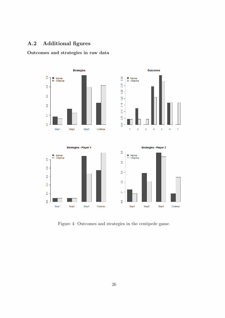
8Similar conclusions can be drawn when considering strategies for player 1 and 2 separately (see Figure
4 in Appendix A.2).
7

Player type Node Elicited belief
Ingroup Outgroup
1
21.33 1.54
(2.76) (3.59)
43.54 3.42
(3.68) (3.74)
67.29 9.13
(3.94) (3.50)
2
11.96 1.33
(4.18) (3.07)
33.42 3.13
(4.09) (3.30)
59.00 8.33
(3.15) (3.25)
Notes: Average number of subjects, out of 12,
guessed to stop at each node (by player type and
treatment). Standard deviation in parentheses.
Table 1: Elicited beliefs.
To summarize, group identity manipulations have previously been shown to strengthen
social preferences (i.e. increase altruism, propensity to positively reciprocate, and desire
for social-welfare maximization), but we find no evidence of this in our study: actions
differ in the opposite way to that implied by a long line of research into the effect of group
identity on social preferences, while reported beliefs do not differ systematically between
treatments.
3.2 Reactiveness to stated beliefs
This section investigates the underlying decision-making process (captured by first-order
beliefs and the resulting action-belief correspondence) of players based on their group
affiliation. The OLS regressions in Table 2 provide initial evidence that subjects in the
ingroup treatment act much more upon their reported beliefs than subjects in the outgroup
treatment.9
9The purpose of this section is primarily to demonstrate a clear pattern in the data in a simple way
to justify the more complex approach in the following subsection. Because these regressions are only for
illustrative purposes, and properly reporting non-linear models with interaction effects is more elaborate,
8

Model 1 Model 2 Model 3
Belief 0.041∗∗∗ 0.041∗∗∗ 0.028∗∗
(0.006) (0.006) (0.008)
Ingroup –0.091∗∗ –0.288∗∗∗
(0.045) (0.110)
Inbelief 0.028∗∗∗
(0.011)
Constant 0.504∗∗∗ 0.549∗∗∗ 0.643∗∗∗
(0.060) (0.063) (0.079)
R2 0.209 0.222 0.246
Notes: Standard errors in parentheses are clustered by sub-
ject. All estimations with 240 observations. ∗∗∗ significant
at the 1% level, ∗∗ significant at the 5% level, ∗ significant
at the 10% level.
Table 2: Probability of continuing estimated by linear probability model.
Model 1 controls for the beliefs about the number of players that will continue at the
subsequent decision node. Including this variable as a regressor, we lose the observations
of player 2s’ final decision node, as there are no subsequent decisions. Results show that
the subjects’ beliefs have a positive impact on their own decision to continue, significant
at the 1% level. Subjects respond in a rational direction to their stated beliefs, that is the
more likely they believe it is that their partner will continue at the next node, the less
likely they are to stop.
An alternative approach to looking for a social preference effect is to test for a treatment
difference in the probability of stopping after controlling for beliefs. Model 2 therefore
includes a dummy for the ingroup treatment. The coefficients imply that subjects with the
same beliefs about the probability of their partner stopping at the next node are almost
10% less likely to continue if matched with an ingroup member. This result goes against
the social preferences hypothesis, and is significant at the 5% level.
Model 3 adds an interaction term between the elicited belief and the ingroup treat-
ment dummy to allow for the possibility that the relationship between reported beliefs
and actions differs between treatments. The estimated coefficients are all significant and
imply that the relationship between beliefs and actions is twice as strong in the ingroup
treatment. Using the estimated coefficients of this model, Figure 3 nicely illustrates the
large differences in the reactiveness to beliefs between treatments: behavior of subjects
we report here linear regressions only. Probit and logit regressions however yield similar results and are
available upon request.
9
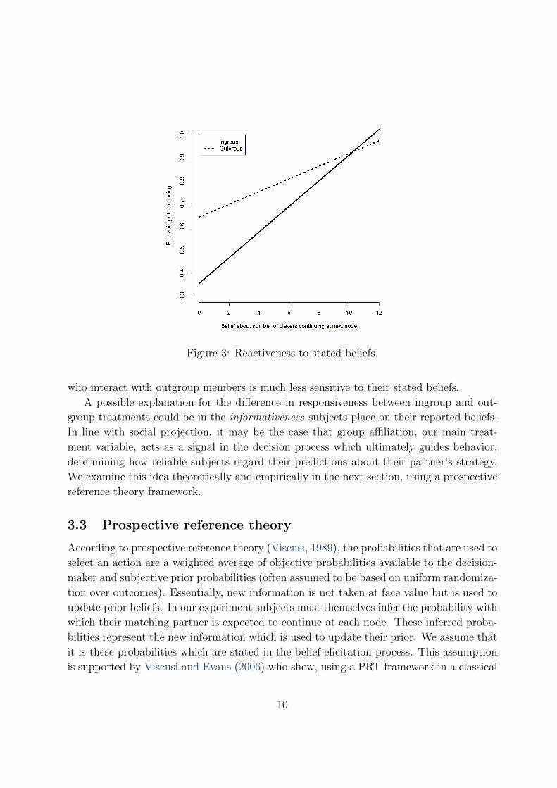
Figure 3: Reactiveness to stated beliefs.
who interact with outgroup members is much less sensitive to their stated beliefs.
A possible explanation for the difference in responsiveness between ingroup and out-
group treatments could be in the informativeness subjects place on their reported beliefs.
In line with social projection, it may be the case that group affiliation, our main treat-
ment variable, acts as a signal in the decision process which ultimately guides behavior,
determining how reliable subjects regard their predictions about their partner’s strategy.
We examine this idea theoretically and empirically in the next section, using a prospective
reference theory framework.
3.3 Prospective reference theory
According to prospective reference theory (Viscusi, 1989), the probabilities that are used to
select an action are a weighted average of objective probabilities available to the decision-
maker and subjective prior probabilities (often assumed to be based on uniform randomiza-
tion over outcomes). Essentially, new information is not taken at face value but is used to
update prior beliefs. In our experiment subjects must themselves infer the probability with
which their matching partner is expected to continue at each node. These inferred proba-
bilities represent the new information which is used to update their prior. We assume that
it is these probabilities which are stated in the belief elicitation process. This assumption
is supported by Viscusi and Evans (2006) who show, using a PRT framework in a classical
10

situation of decision-making under uncertainty, that reported probabilities are indeed only
partially informative about “behavioral” probabilities (defined as the probabilistic belief
consistent with observed choices). The inferred probabilities, as proxied by the elicited
beliefs, will be viewed as more informative when the partner is considered to be more like
oneself, i.e. an ingroup rather than outgroup member.10
We will now consider a model based on prospective reference theory that can capture
the differences in the reliability of a player’s beliefs of the partner’s behavior that we observe
in our experimental data. Assume that the utility function exhibits constant relative risk
aversion (CRRA), u (x) = x1−r
1−r , where x denotes the realized payoff in the game and r
the degree of risk aversion.11 Each subject has the choice to stop (S) or continue (C) at
each of her three decision nodes (1,3,5 for player type 1 and 2,4,6 for player type 2). A
strategy is a vector specifying a choice for each move of player i = 1, 2, e.g. si = (C, S, S).
Since we are only interested in a subject’s first stopping decision for the estimation of
the model, we consider by a slight abuse of notation only the truncated strategy vector,
e.g. si = (C, S, ·).12 According to this truncation, each subject has 4 (pure) strategies
which are to stop at any of her three decision nodes or to always continue. This yields a
total of seven possible outcomes mj, with j ∈ {1, 2, . . . , 7}, and each outcome mj being
associated with a payoff of xi,j to subject i. For the estimation, we assume that subjects
choose a strategy according to a logistic choice function, as specified below.
Define qi,j as the probability of a subject receiving payoff xi,j, given that she plays
strategy si and the other player chooses each of the four strategies with equal probability
(the assumed prior belief). The prior belief is supposed to capture beliefs about the
partner’s actions before any reasoning process has begun. The priors we consider are
both applications of the “principle of insufficient reason”: uniform randomization over
truncated strategies and uniform randomization at each node. We assume the former for
the estimations in this section, but all results are robust to using the latter. For example,
if player 1 chooses to stop at her first node then the only possible outcome of the game is to
end there, that is q1,1 = 1 and q1,j = 0 for j ∈ {2, . . . , 7}.13 Denote by pi,j the probability
of the outcome associated with payoff xi,j given the subject’s inferred probabilities and the
choice si. Let the weight the subject places on the assumed prior be 0 ≤ α ≤ 1. The term
10Rutstrom and Wilcox (2009) also find that stated beliefs do not predict future actions as well as
behavioral probabilities. Note that what they define as “inferred probabilities” are not related to what we
define as such, but are conceptually equivalent to our behavioral probabilities.11All results are robust to using a CARA utility function u(x) = −exp(a x), where a is the degree of
absolute risk aversion.12Only 3 (out of 96) subjects chose a strategy involving a choice to continue after a choice to stop, so
this truncation is of little practical consequence.13As another example, suppose that player 1 chooses to stop at the third node. Then the game terminates
at node 2 if player 2 chooses to stop there, or at node 3 if player 2 chooses a strategy that plays continue
at node 2, so q1,2 = 14 , q1,3 = 3
4 , and q2,j = 0 for j ∈ {1, 4, 5, 6, 7}.
11

1 − α captures the “subjective informational content” of the inferred beliefs, with α = 0
implying that their reported belief is regarded as fully informative by the subject. We
allow this weight to differ between treatments, by replacing α for the ingroup treatment
by α + αOUT for the outgroup treatment.
The utility function subject i maximizes when choosing her strategy si can then be
written as,
PRT (si) =7∑j=1
((α + αOUT ) qi,j + (1− α− αOUT ) pi,j)u (xi,j) . (1)
As has become standard in the literature, we assume the probability a player chooses
strategy si is given by the following logistic choice function,
Pr (si) =eλPRT (si)∑4k=1 e
λPRT (sk)(2)
where λ ≥ 0 represents the degree of rationality (or sensitivity to payoff differences) of the
player. Note that this model encompasses expected value (for r = 0 and α = αOUT = 0)
and expected utility (for α = αOUT = 0) as special cases. The parameters of interest are
estimated using a maximum likelihood estimation, with the log likelihood, given by
ln L (λ, r, α, αOUT ) =N∑i=1
ln Pr (si) . (3)
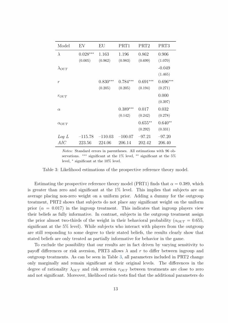
Table 3 summarizes results for expected value (EV), expected utility (EU), and various
PRT specifications.14 The coefficient on λ in the EV model is significantly different from
zero at the 1% level which confirms that subjects are not acting randomly.15
The standard subjective expected utility model (EU) allows for risk aversion and yields
a much better overall fit than the EV model. Estimates of the coefficient of relative risk
aversion r range between 0.830 in the EU and 0.691 in the PRT models; the relatively high
estimates (cf. Holt and Laury, 2002) might be due to the exponentially-increasing payoffs
in the game and the salience of possibly large monetary earnings that come with them.
14As an estimate for the subjective probability of the partner choosing to stop at a given node we use
the proportion of subjects guessed to stop at that node. Theoretically, this is always within an interval
of size 1/13 of the true subjective probability (see Hurley and Shogren, 2005). Our results are robust to
using the minimum, maximum, and mid-point of the elicited interval.15Estimates of λ are much higher in all other models of Table 3, i.e. indicative of a greater level of
rationality, but with much greater standard errors and thus are not significant. We are however confident
that λ is greater than zero because λ = 0 implies the model collapses to the random model regardless of
the other parameter values, and likelihood ratio tests (in Table 4) show that all the models in Table 3
perform significantly better than the random model at the 1% level.
12
Model EV EU PRT1 PRT2 PRT3
λ 0.028∗∗∗ 1.163 1.196 0.862 0.906
(0.005) (0.962) (0.983) (0.699) (1.070)
λOUT -0.049
(1.465)
r 0.830∗∗∗ 0.784∗∗∗ 0.691∗∗∗ 0.696∗∗∗
(0.205) (0.205) (0.194) (0.271)
rOUT 0.000
(0.397)
α 0.389∗∗∗ 0.017 0.032
(0.142) (0.242) (0.278)
αOUT 0.655∗∗ 0.640∗∗
(0.292) (0.331)
Log L –115.78 –110.03 –100.07 –97.21 –97.20
AIC 223.56 224.06 206.14 202.42 206.40
Notes: Standard errors in parentheses. All estimations with 96 ob-
servations. ∗∗∗ significant at the 1% level, ∗∗ significant at the 5%
level, ∗ significant at the 10% level.
Table 3: Likelihood estimations of the prospective reference theory model.
Estimating the prospective reference theory model (PRT1) finds that α = 0.389, which
is greater than zero and significant at the 1% level. This implies that subjects are on
average placing non-zero weight on a uniform prior. Adding a dummy for the outgroup
treatment, PRT2 shows that subjects do not place any significant weight on the uniform
prior (α = 0.017) in the ingroup treatment. This indicates that ingroup players view
their beliefs as fully informative. In contrast, subjects in the outgroup treatment assign
the prior almost two-thirds of the weight in their behavioral probability (αOUT = 0.655,
significant at the 5% level). While subjects who interact with players from the outgroup
are still responding to some degree to their stated beliefs, the results clearly show that
stated beliefs are only treated as partially informative for behavior in the game.
To exclude the possibility that our results are in fact driven by varying sensitivity to
payoff differences or risk aversion, PRT3 allows λ and r to differ between ingroup and
outgroup treatments. As can be seen in Table 3, all parameters included in PRT2 change
only marginally and remain significant at their original levels. The differences in the
degree of rationality λOUT and risk aversion rOUT between treatments are close to zero
and not significant. Moreover, likelihood ratio tests find that the additional parameters do
13

EV EU PRT1 PRT2 PRT3
EV · 0.00 0.00 0.00 0.00
EU · 0.00 0.00 0.00
PRT1 · 0.02 0.12
PRT2 · 0.99
PRT3 ·Notes: p-values.
Table 4: Likelihood ratio tests for nested models.
not significantly improve the fit, but that PRT2, with an outgroup dummy on the weight
assigned to the prior belief αOUT , performs significantly better than all other nested models
(cf. Table 4).
In summary, the estimation results of the PRT model reveal that participants perceive
own stated beliefs as much less relevant for behavior when facing an outgroup member.
Conversely, subjects behave as though their stated beliefs are fully informative when the
partner is considered to be similar to oneself, i.e. an ingroup member. We interpret the
large differences in the informativeness of own stated beliefs that do exist between treat-
ments as evidence that subjects face a much higher degree of uncertainty when predicting
strategic behavior of an unknown, outgroup player relative to an ingroup player. This
finding is consistent with evidence in psychology that social projection, in the sense of per-
ceived similarity and hence predictability of others, is stronger in ingroup than in outgroup
interactions (Acevedo and Krueger, 2005; Ames et al., 2011).
4 Discussion
In our experiment, subjects continue slightly longer with outgroups and they are more
likely to choose to continue with outgroups even if their stated beliefs indicate a high
probability that their partner will stop at the next node. We have argued that uncertainty
about outgroup behavior together with the exponentially-increasing payoff structure in the
game, explain our main findings. In this section, we briefly explore alternative explanations,
including more complex social preferences and limited cognition, that may have contributed
to subjects continuing longer in the outgroup treatment.
Theoretically, fairness between ingroup members could be a concern in the game as
the absolute (but not relative) difference between payoffs increases at each node. Given
the large potential welfare gains, we believe nevertheless that altruism and social-welfare
maximization effects would substantially outweigh any fairness-related concerns, as was
14
found to be the case in the games investigated by Charness and Rabin (2002). Moreover,
the combination of theoretical results from Ho and Su (2013) and empirical estimations
in Kranton et al. (2012) support our intuition. Using the utility function of the inequity
aversion model of Fehr and Schmidt (1999), Ui(xi, xj) = xi − α [xi − xj]+ − β [xj − xi]+
where xi and xj is the monetary payoff of player i and j respectively, Ho and Su (2013)
show that if players are sufficiently averse to having a lower payoff than the other player
(high β) they will stop, whereas if they are sufficiently averse to having a higher payoff
(high α) they will continue all the way. Employing a Klee-Kandinsky manipulation similar
to ours, Kranton et al. (2012) estimate that α is substantially higher and β substantially
lower for subjects interacting with ingroups. Thus, the impact of group identity on fairness
concerns should, if anything, cause players to continue longer with ingroups.
Alternatively, one may also argue that players may feel more disappointed at being
“betrayed” by members of the same group and stop earlier to avoid this potential disap-
pointment, or outgroup members are rewarded more (in anticipation) because nice behavior
from them is more unexpected. This reasoning however is not in line with previous labora-
tory evidence finding stronger positive reciprocity with ingroups and negative reciprocity
stronger with outgroups (Chen and Li, 2009). In short, we do not think that more complex
social preferences explain our results.
In contrast to social-preference based arguments, the experimental literature has fo-
cussed on limited cognition as an explanation for the systematic deviations from the
backward-induction solution.16 We discuss two alternative models of boundedly ratio-
nal behavior, the agent quantal response equilibrium model (AQRE) and the level-k model
and compare their performance to the PRT model presented in Section 3.
In an AQRE model, players are expected to commit mistakes in their decisions. More
specifically, the probability of a particular strategy being chosen is increasing in the ex-
pected payoff to that strategy. The parameter λ in the logistic choice function can be
interpreted as the propensity of a player committing errors, with a value of zero indicating
no relationship between beliefs and actions, and a value of infinity implying that the agent
best-responds perfectly. Errors, committed by the player at different decision nodes, are
assumed to be independent and realized only when the respective node is reached (see Ap-
pendix A.1 for details on the specifications). Table 5 reports the estimates for the AQRE.
16Palacios-Huerta and Volij (2009) find that subjects stop sooner when playing chess players than when
playing students, and Bornstein et al. (2004) show that games tend to stop earlier when decisions are
made by groups than by individuals. These results are explained in the respective papers by chess-players
being better at backward induction than students, and groups behaving more rationally than individuals.
Note that Levitt et al. (2011) however find no such clear relation between the ability to perform backward
induction (measured in a “race to 100” game) and behavior of chess players in the centipede game.
Gerber and Wichardt (2010) use an “enriched” centipede game (which includes insurance options against
termination of the game by the partner or reward options for not terminating the game) and explain their
results by a process of limited iterated reasoning of players.
15

Model Data λ φ Log L AIC
AQREIngroup 0.044 –66.68
282.24Outgroup 0.030 –73.44
AQRE+ALTIngroup 0.076 0.057 –60.50
251.52Outgroup 0.048 0.103 –63.26
Table 5: Agent quantal response estimations in the standard model (AQRE) and in the
model allowing for a proportion of altruists (AQRE+ALT).
The degree of rationality λ is smaller in the outgroup treatment, suggesting subjects make
more errors when interacting with outgroups, consistent with our regression results in Sec-
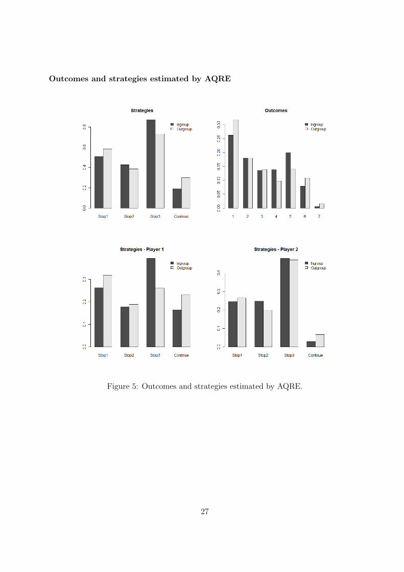
tion 3.3. However, as is clear from a comparison of Figures 2 and 5, this model fits the
data poorly. We also follow McKelvey and Palfrey (1992) and test whether a proportion
of altruists φ in the population, who are assumed to always play continue, improves the fit
of the model (AQRE+ALT), but find a much higher fraction of altruists in the outgroup
than in the ingroup treatment which contradicts a strong prior about the impact of group
identity on social preferences. Finally, the performance of both models in terms of the
Akaike Information Criterion (AIC) is inferior to the PRT model in Section 3.3.
In a level-k model subjects are assumed to be of one of a hierarchy of types, reflecting
differences in their depths of reasoning (first introduced in Stahl and Wilson, 1994, 1995;
Nagel, 1995). Level zero (L0) is defined exogenously, whereas higher levels best respond
to their beliefs, possibly with some noise. Following Kawagoe and Takizawa (2012), we
consider a level-k model of the centipede game with three different level zero types (L0):
random normal form (RNF), random behavioral strategy (RBS), and altruists (ALT) who
are assumed to always continue (for specifications refer to Appendix A.1).
Table 6 summarizes our level-k estimates. We find large differences between the distri-
butions of cognitive levels in our two treatments, with subjects tending to be categorized
as lower levels in the outgroup treatment. This holds for all of the three L0 specifications
considered. The large number of unsophisticated L1 subjects in the outgroup treatment is
intuitively appealing if outgroup member are perceived as less sophisticated than ingroup
members, which is in line with the idea that group affiliation is aimed at increasing self-
esteem. However, in a level-k model differences in behavior can result only from differences
in beliefs, whereas the beliefs we have elicited do not differ between treatments. This rules
out the possibility that the level-k estimates can explain the totality of our results, even
though such estimates fit the data quite well (comparing estimated strategies to the empir-
ical strategies, see Appendix A). We take the rather extreme shifts of the type distribution
towards L1s in the outgroup treatment as further evidence that these players find it more
16

Model Data Level 1 Level 2 Level 3 Level 4 λ Log L AIC
RNFIngroup 0.31 0.25 0.41 0.03 0.056 -55.18
223.60Outgroup 0.66 0.11 0.22 0.00 0.047 -52.68
RBSIngroup 0.44 0.25 0.29 0.02 0.076 -52.08
223.46Outgroup 0.77 0.11 0.13 0.00 0.083 -52.71
ALTIngroup 0.26 0.12 0.60 0.02 0.050 -51.92
223.82Outgroup 0.45 0.00 0.55 0.00 0.032 -53.05
Table 6: Estimation results of level-k model.
difficult to predict the behavior of their matching partner and are more likely to assume
they act randomly. Moreover, the PRT model is also preferred based on the AIC.
Given that the assignment to treatments was random, there is no convincing reason
why the cognitive ability of subjects playing outgroups should be lower than those playing
ingroups. Level-k estimations however illustrate nicely how the sophistication of play
changes with group affiliation in the game. In this respect, our level-k results support
recent work suggesting that level-k reasoning can also be interpreted as beliefs about others
(Georganas et al., 2013; Burchardi and Penczynski, 2011; Agranov et al., 2012).17
More generally, the PRT estimates and the results in the discussion show that strategic
sophistication is a function of the environment and can be manipulated, as in our case,
through changes in group affiliation. The result that subjects’ reasoning depends on the
group affiliation is also consistent with a recent neuroscientific study of Baumgartner et al.
(2012) which identifies differences in the activation of the mentalizing system (a region
associated with social reasoning or projection in the brain) of subjects when facing ingroup
and outgroup behavior.
5 Conclusion
This paper tested the hypothesis that social preferences drive behavior in the one-shot
centipede game. We used a group identity manipulation (cf. Tajfel and Turner, 1979; Chen
and Li, 2009) which has been shown in various economic settings to increase altruism, the
propensity to positively reciprocate and the desire for social-welfare maximization. We
17Georganas et al. (2013) find that subjects’ levels are largely uncorrelated with an assortment of cogni-
tive ability tests and that subjects perform as higher types when they know that they are playing with a
subject who has performed well in those tests. Moreover, both Georganas et al. (2013) and Burchardi and
Penczynski (2011) show that subjects’ estimated levels vary unsystematically across different types and
even small variations of games. Agranov et al. (2012) find that subjects’ cognitive levels are endogenous,
i.e. influenced by the beliefs they hold about their opponents’ cognitive ability.
17
found no evidence that the effect of strengthened social preferences plays a decisive role for
behavior in the centipede game. On the contrary, participants interacting with outgroup
members continue longer and earn significantly higher payoffs than those playing members
of the own group.
In the analysis of the game we allowed for the possibility that group identity not only
affects own and others’ payoffs through changes in preferences, as posited by theoretical
work (Akerlof and Kranton, 2000; Shayo, 2007), but also impacts a player’s social reasoning
about her partner’s behavior, e.g. through social projection (Acevedo and Krueger, 2005;
Ames et al., 2011). Depending on the game’s structure and the complexity of the strategic
environment, these two forces can have countervailing effects on behavior.
Given the exponentially-increasing payoff structure in the one-shot centipede game we
considered, a player should only stop if she is sufficiently confident that her partner will
stop at the next node. To explicitly account for the underlying uncertainty about the
other player’s behavior in the introspection process we estimated a prospective reference
theory model. Results showed that subjects playing an ingroup member treat stated first-
order beliefs as much more informative than those playing an outgroup member. That
is, subjects relied in ingroup interactions much more on their assessment of the partner’s
predicted behavior than in outgroup interactions. Moreover, our finding that strategic
sophistication of participants, e.g. in level-k models, varies strongly in group affiliation is
in full accordance with our interpretation of results. In summary, our research shows that
group affiliation influences not only social preferences of players but also their underlying
reasoning processes.
References
Acevedo, Melissa and Joachim I. Krueger (2005), “Evidential reasoning in the prisoner’s
dilemma.” The American Journal of Psychology, 118, 431–457.
Agranov, Marina, Elizabeth Potamites, Andrew Schotter, and Chloe Tergiman (2012),
“Beliefs and endogenous cognitive levels: an experimental study.” Games and Economic
Behavior, 75, 449–463.
Akerlof, George A. and Rachel E. Kranton (2000), “Economics and identity.” Quarterly
Journal of Economics, 115, 715–753.
Ames, Daniel R., Elke U. Weber, and Xi Zou (2011), “Mind-reading in strategic interac-
tion: The impact of perceived similarity on projection and stereotyping.” Organizational
Behavior and Human Decision Processes, 117, 96–110.
18

Aumann, Robert J. (1995), “Backward induction and common knowledge of rationality.”
Games and Economic Behavior, 8, 6–19.
Aumann, Robert J. (1998), “On the centipede game.” Games and Economic Behavior, 23,
97–105.
Ayres, Ian (1991), “Fair driving: Gender and race discrimination in retail car negotiations.”
Harvard Law Review, 104, 817–872.
Baumgartner, Thomas, Lorenz Gotte, Rahel Gugler, and Ernst Fehr (2012), “The mental-
izing network orchestrates the impact of parochial altruism on social norm enforcement.”
Human Brain Mapping, 33, 1452–1469.
Blanco, Mariana, Dirk Engelmann, Alexander K. Koch, and Hans-Theo Normann (2012),
“Preferences and beliefs in a sequential social dilemma: A within-subjects analysis.”
Working Paper.
Bornstein, Gary, Tamar Kugler, and Anthony Ziegelmeyer (2004), “Individual and group
decisions in the centipede game: Are groups more “rational” players?” Journal of Ex-
perimental Social Psychology, 40, 599–605.
Brandts, Jordi and Gary Charness (2011), “The strategy versus the direct-response
method: a first survey of experimental comparisons.” Experimental Economics, 14, 375–
398.
Burchardi, Konrad B. and Stefan P. Penczynski (2011), “Out of your mind: Eliciting
individual reasoning in one shot games.” Working Paper.
Charness, Gary and Mathew Rabin (2002), “Understanding social preferences with simple
tests.” Quarterly Journal of Economics, 117, 817–869.
Chen, Roy and Yan Chen (2011), “The potential of social identity for equilibrium selec-
tion.” American Economic Review, 101, 2562–2589.
Chen, Yan and Xin Li (2009), “Group identity and social preferences.” American Economic
Review, 99, 431–457.
Costa-Gomes, Miguel A. and Vincent P. Crawford (2006), “Cognition and behavior in
two-person guessing games: An experimental study.” American Economic Review, 96,
1737–1768.
Engelmann, Dirk and Martin Strobel (2012), “Deconstruction and reconstruction of an
anomaly.” Games and Economic Behavior, 76, 678–689.
19
Fehr, E. and K. M. Schmidt (1999), “A theory of fairness, competition, and cooperation.”
Quarterly Journal of Economics, 114.
Fey, Mark, Richard D. McKelvey, and Thomas R. Palfrey (1996), “An experimental study
of constant-sum centipede games.” International Journal of Game Theory, 25, 269–287.
Fischbacher, Urs (2007), “z-tree: Zurich toolbox for ready-made economic experiments.”
Experimental Economics, 10, 171–178.
Georganas, Sotiris, Paul J. Healy, and Roberto A. Weber (2013), “On the persistence of
strategic sophistication.” Working Paper.
Gerber, Anke and Philipp C. Wichardt (2010), “Iterated reasoning and welfare-enhancing
instruments in the centipede game.” Journal of Economic Behavior & Organization, 74,
123–136.
Goeree, Jacob and Charles A. Holt (2004), “A model of noisy introspection.” Games and
Economic Behavior, 46, 365–382.
Goette, Lorenz, David Huffman, and Stephan Meier (2012a), “The impact of social ties on
group interactions: Evidence from minimal groups and randomly assigned real groups.”
American Economic Journal: Microeconomics, 4, 101–115.
Goette, Lorenz, David Huffman, Stephan Meier, and Matthias Sutter (2012b), “Competi-
tion between organizational groups: Its impact on altruism and antisocial motivations.”
Management Science, 58, 948–960.
Graddy, Kathryn (1995), “Testing for imperfect competition at the Fulton fish market.”
RAND Journal of Economics, 26, 75–92.
Ho, Teck-Hua and Xuanming Su (2013), “A dynamic level-k model in sequential games.”
Management Science, 59, 452–469.
Holt, Charles A. and Susan K. Laury (2002), “Risk aversion and incentive effects.” Amer-
ican Economic Review, 92, 1644–1655.
Hurley, Terrance M. and Jason F. Shogren (2005), “An experimental study of induced and
elicited beliefs.” Journal of Risk and Uncertainty, 30, 169–188.
Kawagoe, Toshiji and Hirokazu Takizawa (2012), “Level-k analysis of experimental cen-
tipede games.” Journal of Economic Behavior & Organization, 82, 548–566.
Kranton, Rachel E., Matthew Pease, Seth Sanders, and Scott Huettel (2012), “Identity,
group conflict, and social preferences.” Working Paper.
20

Krueger, Joachim I. (2007), “From social projection to social behaviour.” European Review
of Social Psychology, 18, 1–35.
Krueger, Joachim I., Theresa E. DiDonato, and David Freestone (2012), “Social projection
can solve social dilemmas.” Psychological Inquiry, 23, 1–27.
Levitt, Steven D., John A. List, and Sally E. Sadoff (2011), “Checkmate: Exploring back-
ward induction among chess players.” American Economic Review, 101, 975–990.
Li, Sherry Xin, Kutsal Dogan, and Ernan Haruvy (2011), “Group identity in markets.”
International Journal of Industrial Organization, 29, 104–115.
Manski, Charles F. (2004), “Measuring expectations.” Econometrica, 72, 1329–1376.
McKelvey, Richard D. and Thomas R. Palfrey (1992), “An experimental study of the
centipede game.” Econometrica, 60, 803–836.
McKelvey, Richard D. and Thomas R. Palfrey (1995), “Quantal response equilibria for
normal form games.” Games and Economic Behavior, 10, 6–38.
McKelvey, Richard D. and Thomas R. Palfrey (1998), “Quantal response equilibria for
extensive form games.” Experimental Economics, 1, 9–41.
Nagel, Rosemarie (1995), “Unraveling in guessing games: an experimental study.” Ameri-
can Economic Review, 85, 1313–1326.
Nagel, Rosemarie and Fang Fang Tang (1998), “Experimental results on the centipede game
in normal form: An investigation on learning.” Journal of Mathematical Psychology, 42,
356–384.
Palacios-Huerta, Ignacio and Oscar Volij (2009), “Field centipedes.” American Economic
Review, 99, 1619–1635.
Rapoport, Amnon, William E. Stein, James E. Parco, and Thomas E. Nicholas (2003),
“Equilibrium play and adaptive learning in a three-person centipede game.” Games and
Economic Behavior, 43, 239–265.
Robbins, Jordan M. and Joachim I. Krueger (2005), “Social projection to ingroups and
outgroups: A review and meta-analysis.” Personality and Social Psychology Review, 9,
32–47.
Rosenthal, Robert W. (1981), “Games of perfect information, predatory prices and the
chain-store paradox.” Journal of Economic Theory, 25, 92–100.
21

Rutstrom, Elisabet and Nathaniel T. Wilcox (2009), “Stated beliefs versus inferred beliefs:
A methodological inquiry and experimental test.” Games and Economic Behavior, 67,
616–632.
Selten, Reinhard (1967), “Die Strategiemethode zur Erforschung des eingeschrankt ra-
tionalen Verhaltens im Rahmen eines Oligopolexperiments.” In Beitrage zur experi-
mentellen Wirtschaftsforschung (H. Sauermann, ed.), 136–168, Mohr.
Shayo, Moses (2007), “A theory of social identity with an application to redistribution.”
Working Paper.
Stahl, Dale O. and Paul W. Wilson (1994), “Experimental evidence on players’ models of
other players.” Journal of Economic Behavior & Organization, 25, 309–327.
Stahl, Dale O. and Paul W. Wilson (1995), “On players’ models of other players: Theory
and experimental evidence.” Games and Economic Behavior, 10, 218–254.
Tajfel, Henri and John Turner (1979), The Social Psychology of Intergroup Relations, chap-
ter 3: An Integrative Theory of Intergroup Conflict. Brooks-Cole.
Viscusi, W. Kip (1989), “Prospective reference theory: Toward an explanation of the
paradoxes.” Journal of Risk and Uncertainty, 2, 235–263.
Viscusi, W. Kip and William N. Evans (2006), “Behavioral probabilities.” Journal of Risk
and Uncertainty, 32, 5–15.
22

A Appendix: Additional material (for online publi-
cation)
A.1 Specification of alternative models
This section provides some details on the estimation specifications of the agent quantal
response equilibrium model and the level-k model whose results have been discussed in
Section 4.
Agent quantal response
Quantile Response Equilibrium (QRE) is a model for normal-form games that allows for
errors in actions by players but is a fully consistent equilibrium model in that players
correctly adjust their strategy to account for the error structure (McKelvey and Palfrey,
1995). Agent Quantile Response Equilibrium (AQRE), developed by McKelvey and Palfrey
(1998), extends this concept to extensive-form games under the assumption that the errors
made by a player (or agent respectively) at different nodes are independent and realized
only when the node is reached. In the version we estimate, errors are in the form of a logistic
probabilistic choice function, i.e. the probability a player chooses to stop at decision node
j ∈ {1, 2, . . . , 6} is,
pj =eλu(stop)
eλu(stop) + eλu(continue)
where u (.) is the expected utility of choosing a given action, and λ is an error parameter
to be estimated. Note that we interpret λ here as determining the likelihood of making
an error but it can also be interpreted as the sensitivity to payoff differences; the logistic
choice function can also be derived from a latent variable model with random shocks to
preferences. As λ approaches infinity, players best respond to their beliefs, and at zero
players play randomly.
Following McKelvey and Palfrey (1992), we estimate two different specifications of the
model. In the first model (AQRE), all players are assumed to act purely self-interested.
The second model (AQRE+ALT) assumes there is a proportion of altruists φ ∈ [0, 1] in the
population who choose to continue with probability one at each decision node. In the first
model (AQRE) it is straightforward to calculate the stopping probabilities as functions of
λ recursively from the final decision node. The second model (AQRE+ALT) is slightly
more complex as players must update their beliefs about the probability their partner being
an altruist as the game progresses. At the first node, the player type 1 belief about the
proportion of altruists is β1 which equals the prior φ. At the second node, player type 2
23

uses Bayes’ rule to update her belief, which yields
β2 =φ
φ+ (1− φ) (1− p1)
and so on. We thus obtain the equations for the stopping probabilities pj given the beliefs
about the portion of altruists in the population βj at each node, that is
p6 = (1 + exp (−64λ))−1
p5 = (1 + exp(λ[32 (1− β5) p6 + 256 (β5 + (1− β5) (1− p6))− 64])−1
......
...
The log likelihood function is then given by,
LL =6∑j=1
mj ln ((1− φ) pj) + nj ln (φ+ (1− φ) (1− pj))
where mj and nj are the number of subjects who choose to stop or continue at decision node
j, respectively. The estimations were performed by a grid-search method. For each pair
of numbers λ and φ, the system of belief and stopping probability equations were solved
simultaneously, and the log likelihood value was calculated using the resulting stopping
probabilities. Furthermore, we assumed for the estimation that subjects would choose to
stop at all nodes after their first decision to stop (which was the case for all but 3 of our
96 subjects in the data).
Level-k
For the level-k analysis, we follow the basic modeling setup of Kawagoe and Takizawa
(2012), who essentially apply the assumptions of Costa-Gomes and Crawford (2006) to the
centipede game. The only difference to the approach of Kawagoe and Takizawa (2012) is
that we use, for the formation of the log likelihood function, individual strategies rather
than outcomes.
In a level-k model, subjects are assumed to be of one of a hierarchy of types, each
believing (with probability one) that their partner is of the type one level lower. Level
zero (L0) is defined exogenously, see specifications below. Errors in play are modeled by a
logistic choice function, i.e. the probability a player i of (level-k) type t selects strategy skis
pi,t,k =eλu(sk)∑4l=1 e
λu(sl)
where u (sk) is the expected utility of choosing sk, given the player’s belief about their
partner’s (level-k) type, and λ is an error parameter to be estimated. Note that for the
24

purposes of this estimation we are assuming subjects are making their decisions at each
node to conform to a preselected pure strategy (sk) of the game in normal-form (i.e. stop
at first decision node, stop at second decision node, stop at third decision node, or always
continue). We assume that subjects are only of levels one to four, and that the distribution
of types is the same amongst player types one and two. This yields the following log
likelihood function,
LL =2∑i=1
4∑k=1
mi,k ln
(4∑j=1
σj pi,t,k
)(4)
where mi,k is the number of player “i”s choosing strategy sk, and σj is the proportion of
strategy level-k type in the population. We perform estimations for three specifications of
type L0:
1. Random in normal-form (RNF): L0 choose each strategy of the normal-form game
with equal probability, that is select stop or continue at each decision nodes with
probability 14, 1
3, and 1
2at decision nodes one, two, and three respectively.
2. Random in behavioral strategies (RBS): L0 choose stop or continue with equal prob-
ability at each decision node.
3. Altruistic (ALT): L0 always continue.
25
A.2 Additional figures
Outcomes and strategies in raw data
Figure 4: Outcomes and strategies in the centipede game.
26
Outcomes and strategies estimated by AQRE
Figure 5: Outcomes and strategies estimated by AQRE.
27

Outcomes and strategies estimated by level-k (RBS)
Figure 6: Outcomes and strategies estimated by level-k (RBS).
28

B Appendix: Instructions (not for publication)
In the following we provide the English translation of the experimental instructions. Partic-
ipants received instructions regarding the general procedure, the group identity manipulation
and the centipede game. Note that the instructions for the group identity manipulation were
adapted from Chen and Li (2009). Instructions of each part were shown to participants just
prior to the respective part. Instructions in the original language (German) are available
upon request.
General instructions [written]
Welcome to this economic experiment! The experiment in which you are about to partici-
pate is part of a research project on decision-making.
If you have a question, now or during the experiment, please raise your hand and remain
silent and seated. An experimenter will come to you to answer your question in private.
If you read the following instructions carefully, you can earn a considerable amount of
money in addition to the 3 Euro, which you receive just for participating in the exper-
iment. How much money you can earn additionally depends both on your decisions and
the decisions of the other participants.
It is therefore very important that you read these instructions, and all later onscreen
instructions, very carefully.
During the experiment you are not allowed to communicate with the other
participants. Violation of this rule will lead to the exclusion from the experiment and all
payments.
We will not speak of Euros during the experiment, but rather of points. Your whole
income will be calculated in points. At the end of the experiment, the total amount of
points you earned will be converted to Euros at the following rate:
20 Points = 1 Euro.
At the end of the experiment you will be privately and anonymously paid in cash the
amount of points you earned during the experiment in addition to the 3 Euro you receive
for participation.
29

In the following we describe to you the general procedure of the experiment: You will
be asked to make various decisions in two consecutive parts of the experiment. In each of
the 2 parts you can earn points for your decisions. How much points you can earn in each
part will be announced before you have to make your decisions. After all decision-making
parts of the experiment, a questionnaire concludes the experiment.
All the information you require for making decisions in part 1 of the experiment will
be displayed directly on screen. You will receive all the information you require for part 2
of the experiment after completion of part 1 of the experiment.
Instructions for part 1 of the experiment [on-screen]
Welcome to part 1 of the experiment.
In the following you will be shown 5 pairs of paintings by two artists. The paintings
were created by two distinct artists. Each pair of paintings consists of one painting being
made by each artist. For each pair, you are asked to choose the painting you prefer. Based
on the paintings you choose, you (and the other participants) will be classified into one of
two groups.
You will then be asked to answer questions on two more paintings. For each correct
answer, you will earn additional points. You may get help from other members or help
others in your own group while answering the questions.
The composition of the groups remains fixed for the rest of the experiment. That is,
you will be a member of the same group for the whole experiment.
After part 1 has finished, you will be given further instructions about the course of the
experiment.
30

Instructions for part 2 of the experiment [written]
In part 2, you are asked to make decisions. The game depicted below describes a game be-
tween two players who make decisions in turn. This picture will be shown to both players,
called player I and player II. It summarizes all possible decisions players can make as
well as all the points player I and player II can earn in the game depending on its outcome.
Both players (I and II) have on each of their 3 decision nodes, which are depicted by
a circle marked I and II respectively, the possibility to choose either Continue (C) or
Stop (S). This means player I decides between Continue (C) or Stop (S) on the first circle
(read from left) and at all other circles marked with I. Similarly, player II decides between
Continue (C) or Stop (S) on all circles marked with II.
How much points each player earns in the game depends on the decisions of both play-
ers. The points player I and player II receive in each of the possible outcomes of the game,
are depicted in the respective quadratic box below.
General structure of the decisions: The two players (I and II) decide sequentially
and alternately. The game begins at the first circle marked with I (see upper left corner
in the picture) There, player I chooses to play either Continue (C) or Stop (S). If player
I chooses Stop (S), the game ends and player I receives 4 points and player II receives
1 point. If player I chooses on her first circle marked with I to Continue (C) then play
proceeds and it is player II’s turn to decide (see first circle II, read from left in the picture).
Player II then chooses either Continue (C) or Stop (S). If player II chooses Stop (S), the
game ends and player I receives 2 points and player II receives 8 points. If player II chooses
Continue (C), then play proceeds to the next circle marked with I where player I chooses
again between Continue (C) and Stop (S). And so on.
Your decisions: Before you make decisions in this game at the computer screen, you
will be informed about whether you are a player I type or a player II type. Your player
type will be drawn randomly and your type will remain fixed for all decisions. You will
then be asked, separately for each of your three decision nodes, to choose either Continue
31

(C) or Stop (S). Please bear in mind that, at the time of your decisions you do not yet
know the decisions of the other player.
The outcome and your point earning from the game is calculated as follows:
As soon as all players made their decisions, each player I is randomly and anonymously
matched with a player II. All decisions of these two players are then combined to calculate
the outcome of the game and with it the respective point earning of each player. You will
be informed about the outcome and your points in the game after all decisions have been
made. It is therefore important that you made your decision in the game carefully, since
they influence the outcome and the points you earn.
If you have questions regarding the explanation of the game, please raise your hand
now. You will receive all further explanations directly on screen.
32
C Appendix: Sample screenshots (not for publica-
tion)
Figure 7: Sample screenshot of decision in centipede game (game at decision node 2).
Figure 8: Sample screenshot of belief elicitation task (belief about population behavior at
decision node 1).
33