Smart fundmgrsstupidmoney bernhardt

Smart fund managers? Stupid money?

Dan Bernhardt Department of Economics, University of IllinoisRyan J. Davies Finance Division, Babson College

Abstract. We develop a model of mutual fund manager investment decisions near the endof quarters. We show that when investors reward better performing funds with higher cashflows, near quarter-ends a mutual fund manager has an incentive to distort new invest-ment toward stocks in which his fund holds a large existing position. The short-term priceimpact of these trades increase the fund’s reported returns. Higher returns are rewardedby greater subsequent fund inflows which, in turn, allow for more investment distortionthe next quarter. Because the price impact of trades is short term, each subsequent quar-ter begins with a larger return deficit. Eventually, the deficit cannot be overcome. Thus,our model leads to the empirically observed short-run persistence and long-run rever-sal in fund performance. In doing so, our model provides a consistent explanation ofmany other seemingly contradictory empirical features of mutual fund performance. JELclassification: D82, G2, G14

Malins gestionnaires de fonds ? Investisseurs stupides ? Les auteurs developpent un modelede decisions d’investissement des gestionnaires de fonds mutuels pres de la fin d’untrimestre. On montre que quand les investisseurs recompensent les fonds mutuels per-formants en y injectant des ressources additionnelles, vers la fin d’un trimestre, le gestion-naire de fonds a une incitation a inflechir le nouvel investissement vers des actions danslesquelles le fond a une forte position existante. L’impact de ces transactions sur les prixde ces actions a court terme augmente les rendements trimestriels rapportes pour le fond.De meilleurs rendements sont recompenses par un influx d’investissement subsequent, cequi ouvre la porte a encore plus de deflection d’investissement au trimestre suivant. Parce

Richard Martin’s master’s essay under the direction of the first author was a building point forthis research. We greatly appreciate Harvey Westbrook Jr’s significant contributions to earlydrafts. We are also grateful for comments received from two anonymous referees, Chris Brooks,Murillo Campello, Duane Seppi, and seminar participants at Queen’s University, St FrancisXavier University, the Northern Finance Association meetings, the Financial ManagementAssociation European meetings, and the Multinational Finance Society meetings.Email: [email protected]; [email protected]

Canadian Journal of Economics / Revue canadienne d’Economique, Vol. 42, No. 2May / mai 2009. Printed in Canada / Imprime au Canada

0008-4085 / 09 / 719–748 / C© Canadian Economics Association

720 D. Bernhardt and R.J. Davies

que l’impact de ces transactions sur le prix des actions est a court terme, chaque trimestresubsequent commence avec un deficit de rendements plus important. Eventuellement, iln’est plus possible de combler ce deficit. Ce modele permet d’expliquer les observationsempiriques de persistance de mesures de performance du fond a court terme et de ren-versement de la tendance a long terme. Le modele fournit aussi une explication consistantede plusieurs autres caracteristiques apparemment contradictoires notees empiriquementdans la performance des fonds mutuels.

1. Introduction

In this paper, we develop a model of mutual fund manager investment de-cisions near the end of quarters. Our basic intuition can be summarized asfollows. We begin with the well-established observation that investors rewardbetter-performing mutual funds with greater cash inflows. Small improvements inrelative performance can generate large increases in future fund cash inflows.1

Thus, mutual fund managers, whose compensation rises with assets under man-agement, have strong incentives to increase the reported quarterly returns oftheir funds. We show that one method for doing so is for the fund to distort itsend-of-quarter purchases toward stocks in which the fund already holds large po-sitions. The short-term price impact of these trades increases the reported valueof the fund’s existing positions, thereby raising the fund’s end-of-quarter reportedreturns.

A fund’s ability to engage in this distortive end-of-quarter trading is lim-ited by the amount of new cash it has available to invest. Funds with bet-ter past performance receive larger cash inflows and this facilitates more ag-gressive end-of-quarter trading. Of course, this distortion comes at a cost –there is no free lunch. Specifically, the price impacts of these trades eventu-ally decay, decreasing the next quarter’s return, all else equal. However, overtime, to overcome the hangover from past distortive trading, funds must en-gage in ever more distortive trades. Eventually the accumulated hangover provestoo much, leading to the long-run reversals in fund performance found in thedata.

Thus, our model provides a framework for explaining the puzzling empiricalevidence that mutual fund returns exhibit short-run persistence (‘hot and coldhands’) and long-run reversals (past top performing funds become future un-derperformers, even after incorporating their initially superior performance).2 Inaddition, the cost of the investment distortions that we model can help to explain

1 For example, see Chevalier and Ellison (1997), Ippolito (1992), and Sirri and Tufano (1998).2 Extensive evidence of short-term persistence and long-run reversals in the performance of

mutual funds is provided by Hendricks, Patel, and Zeckhauser (1993), Malkiel (1995), Brownand Goetzmann (1995), Gruber (1996), Carhart (1997), Zheng (1999), Wermers (2003), andBollen and Busse (2005).

Smart fund managers? Stupid money? 721

why mutual funds tend to underperform non-managed indexes, despite evidencethat mutual fund managers have some stock picking ability.3

A key component of our model is that the price impact of trades decays overtime. Early in a quarter, fund managers may trade so as to minimize investmentdistortions/price impacts. Later in the quarter, however, enough of the priceimpact persists through the end of the quarter to make it attractive to distortinvestments toward assets in place. An extreme manifestation of this is the practiceof ‘high closing’ – artificially boosting the price of a stock by purchasing sharesjust before the market closes on the last day of the quarter.4

Trades in less liquid stocks generally have greater price impacts. Thus, ourmodel predicts that managers of funds that specialize in less liquid stocks havegreater incentives to distort end-of-quarter investment toward existing holdings.Over time, this behaviour will lead these funds to hold undiversified portfo-lios. This is consistent with the observed high-return volatility of specializedfunds. Our model’s link between short-run fund performance and the concentra-tion of fund portfolios can help to reconcile the findings of Kacperczyk, Sialm,and Zheng (2005) on the performance impact of industry concentration in fundholdings.

Our model suggests that funds may adapt their overall holdings to exploitthe incentives modelled here. For instance, smaller funds may focus more onsmaller, illiquid stocks. In this way, a small fund can be a ‘big fish in a smallpond.’ While the typical trade size of a small fund is too small to have muchinfluence on the price of a large stock, the same trade size can have a largeimpact on prices of less liquid stocks. Similarly, our model predicts that, sinceyounger funds have a more sensitive performance-flow relationship, managersof younger funds have greater incentives to distort investment toward assets inplace.5 Thus, our model predictions are consistent with the empirical findingsof Zheng (1999) and Wermers (2003) that smaller funds exhibit greater short-run persistence in performance and even more dramatic long-run reversals inperformance.

Our model also suggests that mutual funds will tend to be momentum traders –when a mutual fund’s past superior performance is generated by large positionsin well-performing stocks, our model predicts that the mutual fund will continueto increases its positions in those stocks, endogenously generating momentum

3 Wermers, Chen, and Jegadeesh (2000) and Pinnuck (2003) observe that stocks purchased bymutual funds tend to outperform stocks that they sell; yet, on average, actively managed fundsunderperform index funds.

4 John Gilfoyle reports, ‘Nearly everyone seems to agree that high closing is common.’ (Macleans,10 July 2000, 39). For example, the Ontario Securities Commission in its case against RT CapitalManagement, Inc. cites the end of year purchase of 1900 shares of Dia Met at a $.50 premium.A Globe and Mail (7 July 2000) investigation found that in mutual funds on the final trading dayof the year, ‘last-minute leaps beyond the normal market trends strongly suggested a round of“portfolio pumping.”’

5 Chevalier and Ellison (1997) find that younger funds must perform better to attract investment.


through the resulting price impact. Our model also predicts that there will be along-run reversal in performance, that is, that those subsequent purchases willearn low long-run returns. San (2007) documents each of these empirical regu-larities for trading by institutions.

Our model takes investors’ decisions to reward higher short-term returns withlarger cash inflows as given. There is ample empirical evidence documenting thisinvestor behaviour. Our analysis suggests that the best response of investors isnot given by this stimulus-response setup – hence the reference to ‘stupid money’in the title; instead, investors’ optimal investment decisions would need to reflectthe strategic incentives of the fund managers. To endogenize the responses ofindividual investors, we would need to extend our model to include heterogeneityin fund manager ability and integrate learning by investors from mutual fundreturns. Bernhardt and Nosal (2008) do this in a strategically simpler settingwhere a hedge fund manager can augment fund payoffs with zero NPV gamblesof his own design. In our strategically richer setting, it is infeasible to endogenizeboth investor and fund manager behaviour, and the reader should be alert to thepossibility that conclusions about ‘stupid money’ might be changed in such asetting.

The paper proceeds as follows. The next section provides an overview of re-lated literature. Section 3 sets up the economic environment. Section 4 analyzeshow a fund’s existing stock holdings influence its manager’s investment decisionsand derive the consequences of these decisions for persistence in fund returns.Section 5 provides numerical examples. Section 6 concludes. Proofs are in anappendix.

2. Related literature

Gallagher, Gardner, and Swan (2007) use daily trading data of investment man-agers to provide direct evidence of ‘painting the tape’ and show that gamingbehaviour is more likely to occur in smaller stocks, growth stocks, and stocks inwhich the fund has a larger position.

Carhart et al. (2002) provide further extensive empirical support. They findthat funds earn tremendous short-run returns near the end of an evaluationperiod, when trading behaviour has the greatest impact on performance: 80%of funds beat the S&P 500 Index on the last trading day of the year (62% forother quarter-end dates), but only 37% (40% other quarters) do so on the firsttrading day of a new year. This effect is even greater for small-cap funds, whichtrade less liquid stocks: 91% of small-cap funds beat the index at year’s end,and 70% for other quarter-end dates versus 34% for first-quarter trading day.Carhart et al. (2002) reject benchmark-beating hypotheses in favour of strategicbehaviour similar to that motivated here. Consistent with our theory, they findfunds that performed better in the past year earned 42 basis points higher returnson the last trading day and 29 basis points lower on the first trading day than


funds with a worse historical performance. In sum, the data strongly support thehypothesis that fund managers respond to the short-run trading incentives thatwe model, and that they are collectively substantial enough to alter aggregatemarket outcomes.

Indeed, Bernhardt and Davies (2005) find that strategic trading by fund man-agers appears to impact returns on aggregate market indexes, so that measuringthe impact relative to the index, as Carhart et al. (2002) do, understates the totaleffect. Specifically, daily returns of the equally weighted index on the last tradingday of a quarter greatly exceed the daily returns on the first trading day of thesucceeding quarter, and this return difference rises with the share of total equityheld by mutual funds.

Zheng (1999) finds that funds with relatively high returns in one quarter havesignificantly greater returns than the average mutual fund in the next quarter,and relatively worse performers in one quarter generate lower returns than theaverage mutual fund in the next period. Zheng (1999) shows that the performancepersistence is short lived: more than one-quarter into the future, funds that didbetter in the past under perform relative to the average fund, while historicallypoor-performing funds, do better. This reversal in performance is so strong thatcumulative returns of historically better performers fall below those of worseperformers within 30 months.

At the stock-holdings level, Wermers (2003) finds that funds ranked in the topquintile in the prior year (‘past winners’) beat the S&P 500 by 2% in the next year(after accounting for trading costs and expenses). He also finds that past winnersbeat past losers (funds in the prior year’s bottom quintile) by 5% in the nextyear. Wermers (2003) provides empirical support for our theoretical connectionbetween fund flows and trades, showing that flow-related buying drives stockprices up, and that this flow-related buying plays a central role in driving thepersistence in fund performance.

In an insightful paper, Berk and Green (2004) develop a model in whichrational investors learn from a fund’s performance about its manager’s abil-ity and allocate funds accordingly. The Berk-Green model can explain bothwhy money flows into mutual funds with recent better performance and awayfrom those with worse past performance. However, the Berk-Green model alsoimplies that past returns should not predict future performance, which is in-consistent with short-term performance persistence and long-run performancereversals found in the data. Primary contributions of our model are to rec-oncile these empirical observations and to provide explanations for severalfeatures of the mutual fund market not explained by the Berk-Green model,such as why stocks purchased by mutual funds outperform those that theysell, yet, on average, mutual funds underperform the market; and the end-of-quarter return patterns and strategic behaviour documented by Gallagher,Gardner, and Swan (2007), Carhart et al. (2002), and Bernhardt and Davies(2005).


3. The model

3.1. Model detailsConsider a risk-neutral mutual fund manager who can invest in three assets: stockA, stock B, and cash. The fund manager enters quarter t with an existing positionof SAt shares in stock A and SBt shares in stock B. The associated share prices arePAt and PBt. Without loss of generality we assume that PAtSAt ≥ PBtSBt. Cashearns a risk-free return of i, which we normalize to zero.

Firms retain their earnings. Hence, a firm’s stock price is equal to its expecteddiscounted lifetime cash flows. We impose no structure on the timing of cashflows. At the beginning of quarter t, each firm makes an earnings announcementand provides guidance about future cash flows, which causes market participantsto update about firm values. We summarize the earnings announcement andguidance by its implications for the percentage change in firm value, δ j,t, so thatδ j,t Pj,t−1 is the change in expected discounted cash flows.6 Following a signal ofδ j,t, investors update about cash flows, leading to a quarter t stock price for firmj of

Pj,t = Pj,t−1 + δ j,t Pj,t−1. (1)

We assume that in quarter t the fund manager privately learns the next quarter’ssignals, δA,t+1 and δB,t+1, and can trade based on this private information inquarter t before the signals are publicly revealed with certainty at the beginningof quarter t + 1. The joint density distribution of signals across firms is given byg(δA, δB). Thus, in our model, mutual funds are informed traders, whose fullyrational trading decisions can be based on private information, in addition tothe liquidity needs arising from net cash inflows and the strategic considerationof the price impacts of trades on returns. One role of private information in ourmodel is to show that incentives to pump existing holdings can be so strongthat the fund manager actually trades in the opposite direction of his privateinformation.

At the end of quarter t, the fund receives net cash inflows of f (r t), where r t wasthe fund’s portfolio return over quarter t. The only structure that we impose is thatf (r t) is increasing in r t – greater past fund performance raises net cash inflowsfrom investors. Presumably, the performance-flow relation reflects investor beliefsthat fund managers differ in their abilities to identify good investments (Berk andGreen 2004). Here, we do not distinguish fund managers by ability, because suchdifferences can also lead to persistence in performance.

Consistent with the findings of Chan and Lakonishok (1995) and Keim andMadhavan (1997), we assume that a fund manager’s stock purchases have short-term price impacts: the more shares that a fund manager purchases, the greater

6 If δ j,t+1 is not proportional to firm value, then pricing is sensitive to a firm’s choice of sharesoutstanding.


is the short-term price impact. Specifically, a purchase of Ijt > 0 shares in stock jcosts Pjt + �Pjt(Pjt, Ijt) > Pjt per share. We summarize the properties of the priceimpact of Ijt, �Pjt(Pjt, Ijt), later in assumptions A1–A4. We are agnostic as to thefundamentals driving the price impact of Ijt – it could be the fact that institutionaltrades contain information, or that market makers must be compensated for hav-ing to readjust their portfolios, and it takes time to do so. What is key is only thatsuch institutional trading activity has a significant and persistent impact on price.It is important to note that our pricing relation does not preclude the possibilitythat market makers adjust their pricing to reflect the end-of-quarter incentivesof funds;7 or that larger orders impose greater inventory costs on market makers.8

In each quarter t, the timing of events is as follows:

1. Firms announce period earnings and market participants revise expectationsabout the discounted present value of a firm’s cash flows so that stock pricesequal PA,t and PB,t.

2. The fund manager learns δA,t+1 and δB,t+1 and invests available cash to max-imize the fund’s expected period return. Available cash consists of net cashinflows f (r t−1) plus the present value of last period’s cash position Mt−1. Thefund manager can sell shares, but cannot sell shares short or borrow to financestock investments.

3. The fund manager’s private information about next period’s signal, δ j,t+1, isrevealed with (independent) probability, γ , and is not revealed with residualprobability (1 − γ ). We assume that γ ∈ (0, 1), that is, information is onlysometimes revealed to the public. A smaller value of γ reflects less leakage ofinformation between the purchase and the end of the period. Thus, γ captureseither (i) the length of time between the purchase and the end of the quarteror (ii) the probability that private signals will be revealed (because the stock issmaller and hence is followed by fewer analysts) or (iii) a combination of botheffects.

4. End-of-quarter stock prices, P∗At, P∗

Bt, are realized. If the fund manager’sprivate information was revealed,

P∗j t = Pjt + δ j,t+1 Pjt.

If the private information was not revealed,

P∗j t = Pjt + �Pjt(Pjt, Ijt).

7 Bhattacharyya and Nanda (2007) augment a standard single asset static Kyle (1985) model byhaving an informed agent’s objective be the weighted average of (i) a short-run return based onthe price generated by his trade on his holdings of the asset and (ii) the final return on the stock,when market maker’s have a signal about the agent’s pre-trade holdings of the asset. They derivea linear pricing rule that is less sensitive to order flow than the standard model.

8 Hendershott and Seasholes (2007) document that, on average, prices rise when larger orderssubstantially reduce market-maker inventories, before falling subsequently in the next weekwhen market makers re-establish their inventories.


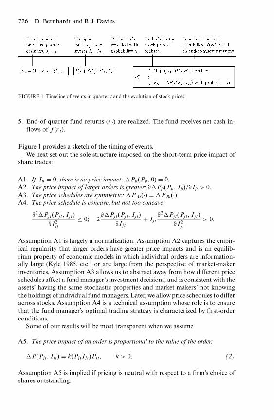
FIGURE 1 Timeline of events in quarter t and the evolution of stock prices

5. End-of-quarter fund returns (r t) are realized. The fund receives net cash in-flows of f (r t).

Figure 1 provides a sketch of the timing of events.We next set out the sole structure imposed on the short-term price impact of

share trades:

A1. If Ijt = 0, there is no price impact: �Pjt(Pjt, 0) = 0.A2. The price impact of larger orders is greater: ∂�Pjt(Pjt, Ijt)/∂ Ijt > 0.A3. The price schedules are symmetric: �PAt(·) = �PBt(·).A4. The price schedule is concave, but not too concave:

∂2�Pjt(Pjt, Ijt)

∂ I2j t

≤ 0; 2∂�Pjt(Pjt, Ijt)

∂ Ijt+ Ijt

∂2�Pjt(Pjt, Ijt)

∂ I2j t

> 0.

Assumption A1 is largely a normalization. Assumption A2 captures the empir-ical regularity that larger orders have greater price impacts and is an equilib-rium property of economic models in which individual orders are information-ally large (Kyle 1985, etc.) or are large from the perspective of market-makerinventories. Assumption A3 allows us to abstract away from how different priceschedules affect a fund manager’s investment decisions, and is consistent with theassets’ having the same stochastic properties and market makers’ not knowingthe holdings of individual fund managers. Later, we allow price schedules to differacross stocks. Assumption A4 is a technical assumption whose role is to ensurethat the fund manager’s optimal trading strategy is characterized by first-orderconditions.

Some of our results will be most transparent when we assume

A5. The price impact of an order is proportional to the value of the order:

�P(Pjt, Ijt) = k(Pjt Ijt)Pjt, k > 0. (2)

Assumption A5 is implied if pricing is neutral with respect to a firm’s choice ofshares outstanding.


Fund manager’s problem. At the beginning of quarter t, the fund manager investsto maximize the expected quarter portfolio return:

maxMt ,IAt ,IBt

E[rt] =Mt +

∑j

Sj,t+1 E[P∗j t]

Mt−1 + f (rt−1) +∑

j

P∗j,t−1Sjt

− 1, (3)

subject to

Mt ≥ 0,

Ijt ≥ −Sjt, j = A, B∑j

[Pjt + �Pjt(Pjt, Ijt)]Ijt + Mt ≤ f (rt−1) + Mt−1,

where Sj,t+1 = Sjt + Ijt and E[P∗jt] = Pjt + (1 − γ ) �Pjt(Pjt, Ijt) + γ δ j,t+1 Pjt.

We will assume that the short-selling constraint, Ijt ≥ − Sjt, j = A, B does notbind: the fund manager does not receive such a bad signal about a stock that hewants to sell more shares of the stock than he has in his portfolio.

3.2. Discussion of the model

3.2.1. Modelling approachThe logical construction of our model is deceivingly simple, masking the fact thatit contains many ingredients that researchers have not yet been able to analyzeeven separately within a structural market microstructure setting. Central to ourmodel is an informed fund manager who is budget constrained, chooses howmany shares of multiple assets to purchase or sell, makes investment decisionsover time, and must incorporate the fund’s existing asset holdings into tradingdecisions. The existing holdings enter non-neutrally because the price impactsof trades affect the portfolio return that investors observe and condition futuremutual fund investments on. Further complicating this dynamic optimizationproblem, a fund manager’s trades must have price impacts, trading scales cannotbe trivial (i.e., zero versus single round lots), and trading rules will be highlynon-linear.

There is a large market microstructure literature dating back to Kyle (1985)that analyzes a single asset that generates endogenously the price impacts of ordersof the form that we model and that are found in the data.9 In Kyle and its multi-agent extensions, risk-neutral speculators receive normally distributed signalsabout one asset’s terminal value, submit orders over time that are mixed in withnormally distributed exogenous ‘noise trade,’ and a market maker sets price equalto the asset’s expected value given the net order flow. The normal assumptionsimply linear conditional forecasts and hence linear pricing, making the problem

9 Noisy rational expectations frameworks are inappropriate here, as they assume that individualsare small, so their individual trades do not generate the price impact found in the data.


solvable. Caballe and Krishnan (1994) extend this analysis to multiple stocks in astatic setting and prove that a linear equilibrium exists. Bernhardt and Taub (2008)provide rich analytical characterizations of the Caballe and Krishnan model, andthey also solve for equilibrium outcomes when speculators can condition theirtrades on prices. To our knowledge, there are no other theoretical papers withmultiple assets and price impacts.

Technically, the biggest challenge to handle in a model with full primitives isthe budget constraint, which destroys linearity of forecasts (and hence prices) inmodels with normally distributed signals. Not only does our fund manager havea budget constraint, but the budget is endogenous, there are multiple risky assets,and assets-in-place critically affect optimal trades. While the budget constraint iscentral to the economics of our results, it is not central to the form of pricing – inany setting where an agent’s trade is ‘large,’ the equilibrium pricing schedule willhave price impacts (larger orders receive higher prices), simply because an agentwith a better signal about an asset buys more and must face an opportunity costof buying more – in the form of a higher price.

One can also derive endogenously the qualitative consequences of introduc-ing an investor who wants to devote resources toward assets in place within anequilibrium model. Bhattacharyya and Nanda (2007; hereafter B-N) do this byadapting Kyle (1985) to consider a single investor who cares about both the in-terim payoff on an existing inventory position on a single risky asset and the finalpayoff. The investor has a two-period horizon. At date 1, the investor receivesa private signal and trades once in a simultaneous batch auction. At date 2, theasset is liquidated at its true value. Thus, the investor’s date 1 trading decisionis based on the NAV of his position at dates 1 and 2; in particular, the investorincorporates the price impact of trading on the value of his existing position atdate 1. As a result, the optimal trade size is linearly related to the size of theexisting position.

In the most general B-N setting, the market maker has a noisy signal of theinvestor’s (normally distributed) existing position. This preserves linear forecastsand hence linear pricing. The investor’s incentives to pump up the value of hisholdings reduce the sensitivity of the equilibrium price schedule to order flow,but the qualitative properties of pricing are otherwise preserved. B-N argue thatthe investor’s incentives to enhance short-term values can explain why closed-end funds trade at a discount to their NAVs. Their model, however, cannot shedlight on any of the issues we study, as it cannot deal with multiple risky assets,the budget constraints of mutual funds, or fund managers with multiple tradingopportunities.

In sum, while some of our assumptions are not grounded in primitive founda-tions, our framework requires only a mild reduced-form structure on pricing. Thispricing structure holds empirically and allows us to get at the key links betweenthe market structure of asset pricing, strategic fund manager behaviour, and port-folio returns, thereby reconciling a host of fundamental empirical regularities infund performance.


3.2.2. Empirical evidence in support of price impact functionKeim and Madhavan (1996) find that the price impact of a block trade,measured as the market-adjusted difference between the closing price on theday prior to the trade and the closing price on the day after the trade, is−1.50% for seller-initiated blocks and 1.60% for buyer-initiated blocks. Chan andLakonishok (1995) measure the price impact of a package of institutional tradesand find that buy packages are associated with a principal-weighted average pricechange of almost 1% from the open on the package’s first day to the close onthe last day. The analogous price change for sell packages is −0.3%. This priceimpact is persistent – for example, five days after the completion of a packagetrade, there is a reversal in returns of only −0.07% for buy packages and 0.10%for sell packages.

Frequently, institutional traders use crossing networks, such as POSIT, or useso-called dark liquidity pools to reduce the price impact of their trades. It wouldbe interesting to investigate empirically whether mutual funds reduce their usageof these alternative trading venues near the end-of-quarters.

3.2.3. Time horizon of fund managerWhile fund manager compensation is proportional to assets under management, afund manager’s expected compensation may depend more on gaining a promotionbased on past fund performance.10 Fund manager turnover is high: Baks (2007)finds that on average about 45% of managers leave or start at a fund in any givenyear and that the average time spent at one fund is about three years (less forsmall company growth funds). To capture these incentives, we suppose that in eachperiod a fund manager invests to maximize end-of-period return. We interpret theperiod’s end as the date at which investors receive fund performance information,which leads them to reallocate investments. Focusing on one-period horizons forfund managers eases the analysis, and the incentive effects highlighted remainpresent with longer horizons.

The one-period horizon in our model is best interpreted as a quarter, since thisis the time horizon most commonly used to evaluate mutual fund performances.Our model does not intend to capture all investment decisions made within thequarter – stock purchases and sales made early in a quarter may be motivatedby reasons not modelled here. The key is only that the portfolio’s end-of-quartercomposition is influenced by the features that we model, and that better pastperforming funds tend to have more cash on hand at the quarter’s end becauseof higher accumulated cash inflows throughout the period. We do not claim thatcash inflows received earlier in the period are held in cash (or a passive equityequivalent); although we do not model it formally, fund managers presumablyinitially allocate that cash based on private information and so on and thenreallocate at quarter’s end to reflect the features that we model. This modelling

10 Hu, Hall, and Harvey (2000) find that promotions are positively related to the fund’s pastperformance and demotions are negatively related to past performance.


assumption is consistent with the empirical results of Alexander, Cici, and Gibson(2007), who show that large fund inflows and outflows influence a fund manager’strades. It is also in the same spirit as the theoretical model of Hugonnier andKaniel (2008), who examine portfolio choices by a mutual fund manager whofaces dynamic fund flows. They show that proportional fees in combination withthe performance-flow relation can cause a manager to distort a fund’s risk profile.

3.2.4. Definition of fully invested fundsMost mutual funds have small cash holdings that largely reflect (i) recent cashinflows from investors that have not yet been invested; and (ii) funds held asan insurance to reduce the transaction costs associated with (stochastic) fundredemptions. Yan (2006) finds that the average cash holdings of U.S. domesticequity mutual funds is about 5.3% of assets and shows that the level of cashholdings is primarily driven by fund flow volatility. In fact, Edelen (1999) findsthat about 70% of all mutual fund trades are to meet investor liquidity demands.Our model does not incorporate such investor liquidity demands, and hence itdoes not contain an insurance role for cash holdings. Consequently, when ourmodel refers to fully invested funds, we are thinking about real-world funds withcash positions no larger than those optimally held as insurance against theirexpected redemptions.

4. Analysis

4.1. Distortion of investment toward existing holdingsThe cost of the fund’s new stock purchases, (I At, I Bt), at period t are

costAt = [PAt + �PAt(PAt, IAt)]IAt (4)

costBt = [PBt + �PBt(PBt, IBt)]IBt. (5)

Differences in signals across stocks may offset the incentives to distort investmenttoward existing holdings; thus, to control for differences in signals, we reverse thesignals when comparing investments in each stock. Specifically, consider twoopposing signal patterns: (δA,t+1 = δ1, δB,t+1 = δ2) and (δA,t+1 = δ2, δB,t+1 =δ1). Let cost12

At denote the cost of optimal investment in stock A under the firstsignal pattern, and cost21

Bt denote the cost of optimal investment in stock B underthe second signal pattern, where optimal investments are determined by the fundmanager’s investment problem in (3). Our first result is

PROPOSITION 1. Given assumptions A1–A5, controlling for differences in informa-tion signals across stocks, the fund manager distorts current purchases toward thestock in which he has a larger existing position: cost12

At > cost21Bt when PAtSAt >

PBtSBt.


The proof follows directly from the first-order conditions of the fund manager’sproblem. Note that proposition 1 does not rule out the possibility that the fundmanager’s private information signal for stock B is so large that it dominates theportfolio pumping incentives to purchase stock A. We can provide a strongerstatement about investment in expectation if the distribution of signals is suchthat the manager is just as likely to get a relatively strong buy/sell signal for stockA as we are for stock B. Formally, we say that the joint density distribution ofinformation signals is symmetric when

g(·, δB = y) = g(δA = y, ·), ∀y. (6)

Adding this symmetry condition yields

COROLLARY 1. If the joint density distribution over the fund manager’s privateinformation signals is symmetric, then in expectation (over possible signals) themanager invests more money on the stock in which he has a larger existingposition.

Corollary 1 follows immediately from integrating over signals pairwise.Proposition 1 presents conditions under which the fund manager distorts his

investment toward assets in which he has larger existing positions. The assumedstructure on the price impact of order flow, �P(Pjt, Ijt), ensures that independentof initial share prices, PAt and PBt, and initial holdings, SAt and SBt, the fundmanager always wants to distort investment toward assets in which he holds largerpositions. The result always holds without this structure (i) if cash inflow is sohigh that the fund manager holds some cash or (ii) if, instead, the fund manager isfully invested in the market, the sufficient condition in proposition 1 always holdsas long as either |PAt − PBt| or |δ1 − δ2| are small enough. Essentially, absentthe structure on �P(Pjt, Ijt), we have to consider second-order effects related tothe relative value of purchases, and these depend on differences in ex ante shareprices and differences in signals.

4.2. The likelihood of information revelationWe now reflect on how the likelihood that the fund manager’s private informationis revealed affects his incentives to distort the fund’s purchases toward existingholdings. Our next result maintains the same structure on the price impact oforder flow, and adds the condition

PASA

PBSB>

1 + δA

1 + δB. (7)

This condition ensures that the difference in existing holdings is large relative tothe difference in information signals.


LEMMA 1. There exists an ε > 0 such that condition (7) holds if δA,t+1 ≤δB,t+1 + ε.

We now derive the implications of condition (7):

PROPOSITION 2. Given assumptions A1–A5, new investment in the fund’s largestexisting holding (stock A) is a decreasing function of the probability γ that infor-mation about asset-value innovations is revealed before the end of the period if andonly if condition (7) holds.

The proof follows from exploring how investment must change in response toa change in γ in order to maintain the first-order condition of the manager’sinvestment problem.

The intuition is as follows. When condition (7) holds, the manager’s privateinformation advantage for buying stock A relative to buying stock B is small (ornegative). In this case, the main incentive for the manager to distort investmentstoward stock A is a portfolio pumping motive. An increase in the likelihood ofinformation revelation decreases the value of portfolio pumping, since with ahigher likelihood the end-of-quarter price will reflect fundamental informationrather than the pumping activity. In contrast, when condition (7) does not hold,the manager has such a large informational advantage for trading stock A thathis primary incentive is to trade aggressively on the basis of this information. Inthis case, the more likely this information is to be revealed prior to the end ofthe quarter (and thereby incorporated into this period’s returns), the greater isthe value of purchasing stock A, so that investment in stock A is an increasingfunction of γ .

Adding symmetry, that is, g(·, δB = y) = g(δA = y, ·), we can extendproposition 2 to consider expected investment, unconditional on the realizationof the signal.

COROLLARY 2. If the joint density distribution over the fund manager’s privateinformation signals is symmetric and the dispersion of signals is sufficiently small,then, unconditionally, expected investment in the stock with the larger existingposition declines with the probability that the fund manager’s private informationis revealed.

A smaller γ represents a lower probability of information leakage. This lowerprobability can reflect both a smaller period of time between the purchase ofstocks and a period’s end for the information to leak out, and it can reflect theobservation that smaller stocks are less actively followed, so that there are fewersources to disseminate the information. Hence, the proposition suggests that fundmanagers distort investment more toward existing holdings in smaller stocks orlater in an evaluation period, where price impacts of trades are more likely topersist.


4.3. The importance of the cash constraintWe have shown that a fund manager distorts investments toward existing stockholdings. Despite this distortion, short-run performance may not be persistent.In particular, we now show that if the fund manager is not fully invested in themarket, then the model cannot generate short-run persistence in fund perfor-mance.

PROPOSITION 3. Suppose P∗j,t−1 = Pjt. If the fund manager optimally does not use

all available cash to invest in stocks (and thereby holds cash at the end of the period)and expected mutual fund returns exceed the risk-free rate, then the mutual fund’speriod returns are a declining function of the cash available to be invested at thebeginning of the period.

The proof follows from recognizing that, when the manager optimally holds acash position, the marginal value of relaxing the fund’s budget constraint (theLagrange multiplier) is equal to the return on cash.

The expected mutual fund return exceeds the risk-free rate either if the fundmanager has non-negative cash available to invest ( f ≥ 0) and stocks do notreceive large negative signals (δ j > δ j ), or if negative cash inflows are offset bysufficiently large positive signals. This is because the fund manager can alwaysearn the risk-free return by investing new fund inflows in cash. In our risk-neutralsetting, it is appropriate to compare mutual fund returns with the risk-free rate.More generally, the rational behaviour of risk-averse investors implies that ex-pected mutual fund returns must exceed a comparable risk-adjusted benchmark.This fact, taken in conjunction with proposition 3, implies that if fund managersare not fully invested in stocks, then the model is inconsistent with the empiricalregularity that returns exhibit short-run persistence. Indeed, in proposition 3 weassume that P∗

j,t−1 = Pjt, so that returns are calculated under the assumption thatthe end-of-period t − 1 share price reflected the value of the firm at that moment;that is, there was no past investment distortion. If f (r t−1) was higher becauseof past investment distortion, this would lead to even more negatively correlatedshort-run returns.

4.4. Short-run persistence and long-run reversalsIn our model, persistence is best interpreted in terms of the persistence of relative(ranked) performance: there is short-run persistence when a highly ranked per-former at t − 1 tends to be highly ranked in t; and lower-ranked performers in t − 1tend to be lower ranked in t. Because we do not model why a given fund’s returnis initially higher (perhaps better past private information), we cannot comparethe absolute levels of returns from one period to the next, but we can determinewhen the factors that we model lead a fund that does relatively better at t − 1 todo better at t, but eventually to do worse over sufficiently longer horizons.

In the context of our model, long-run returns are just the multi-period returnrealized by a sequence of decisions made by a fund manager (or multiple fund


managers). Because short-run returns eventually fall for f (r t−1) sufficiently large,‘Ponzi-schemes’ cannot be supported in the long run.

Our model does not introduce persistence of fund manager ability. Here, wefocus on the incentives to portfolio pump and show that this portion of the storygenerates long-run mean reversion. A reversal in performance means that worstpast performance implies eventual better future performance on a ranking scale.A fund overperforms by more when its rank is higher over the evaluation periodthat we calculate returns; and a fund underperforms by more when its returnrank is lower.

We first show that the model generates short-run persistence in performanceif managers are fully invested in the market. In particular, proposition 4 provesthat, if a fund manager is fully invested, then short-run returns first rise with cashinflows, f (r t−1).

PROPOSITION 4. Suppose P∗j,t−1 = Pjt. Suppose that the fund manager has the

same private information about each stock (δA,t+1 = δB,t+1 = δ) and that he is fullyinvested in stocks (i.e., does not hold a cash position). Then there exists an f ∗ suchthat, for f < f ∗, a higher return last period (and hence a higher f) implies a higherreturn this period; and for f ≥ f ∗, further increases in returns in the previous periodimply a lower current return.

In other words, short-run returns first rise with new funds under management(∂r t/∂ f > 0) for cash inflows sufficiently small, but are a declining functionof new funds for cash inflows sufficiently large. The finding for f < f ∗ is therelevant one, as it implies performance persistence (past higher return impliescurrent higher return; i.e., better past performers continue to perform better).

The persistence documented in proposition 4 is driven precisely by the flow-related buying that pushes up stock prices that Wermers (2003) documents. Ob-serve that ∂r t/∂ f > 0 when f is small even if a fund manager has no privateinformation, so that δ = 0. The intuition for proposition 4 is sharpest whenSAt ∼ SBt and PAt ∼ PBt, in which case I At ∼ I Bt ∼ 0. Then Ijt shares arepurchased at a premium of �P(Pjt, Ijt), so the ‘cost’ �P(Pjt, Ijt)Ijt is only ofsecond order. In contrast, the price impact of the share purchase on returns has afirst-order positive impact of order (1 − γ ) �P(Pjt, Ijt)Sjt.11 The rest of the proofshows that the result extends when a fund manager makes non-trivial offsettinginvestments in the two stocks.12

At date t + 1, δA,t+1 and δB,t+1 are revealed and incorporated into prices,so that, ceteris paribus, greater investment distortions at date t reduce returnsin t + 1 by more. Possibly offsetting this decline is the fact that the period t

11 One can re-interpret proposition 3 in the context of proposition 5 as saying that if it is optimalfor a fund not to be fully invested, then cash inflows are too high relative to private information,so that short-run returns are a decreasing function of f (r t−1).

12 As in proposition 3, we calculate returns using P∗j,t−1 = Pjt, that is, higher values of f (r t−1)

primarily reflect factors other than greater past investment distortion.


investment distortion induced greater cash inflows, f (r t), which, in turn, canfacilitate another round of investment distortion. To derive the impact of pastperformance for long-run returns, one just cumulates short-run returns over time.While high cash inflows in period t of f (r t−1) due to better performance in t − 1lead to higher returns in period t, for short-run returns in the next period t + 1not to fall, the second round of investment distortion must dominate the impactdue to the revelation of δA,t+1 and δB,t+1. For longer-run returns to continue torise, it must be that the higher short-run return from the immediate distortion ofinvestment more than offsets lower returns due to realizing past distortions. Butshort-run returns must eventually decline with cash inflow, so once cash inflowis sufficiently high, this cannot occur: eventually, realizing lower returns fromgreater past distortions must lead to lower long-run returns.

We now consider a fund manager who has no private information, so thatgreater incremental investments in existing positions represent more costly dis-tortions that must eventually be realized in the form of lower returns. It followsthat greater cash inflows in period t must lead to lower long-run returns whencumulated over the period [t, t + τ ], for τ sufficiently large. Combining thisobservation with proposition 4, yields the following proposition, documentingthat the model reconciles both the short-run persistence in fund performanceand the long-run reversal in fund performance documented by Zheng (1999) andWermers (2003).

PROPOSITION 5. Even if a fund manager has no private information, for f (r t−1)sufficiently small, short-run returns are a rising function of f (r t−1), but long-runreturns over [t, t + τ ] are a declining function of f (r t−1), for τ sufficiently large.

Proposition 5 indicates that a better performer in t − 1 will be higher ranked int (on the basis of returns), but lower ranked (on the basis of returns) by somedate τ .

Because the fund manager has no private information, from a long-run per-spective, the optimal stock investment is zero. For τ sufficiently high, long-runreturns are a strictly declining function of f (r t−1), because the price premiumpaid for each share rises with the investment. We show later that τ need not bevery large for long-run returns to fall with f (r t−1).

These results hold even if past returns were so bad that redemptions lead toa net outflow of money from the fund. Then the mutual fund manager mustdisinvest. To minimize the adverse return consequences the fund manager tendsto sell stocks in which he has smaller positions (i.e., the negative price impact fromselling impacts a smaller proportion of his portfolio). Further, in the environmentcharacterized by proposition 5, short-run returns are lower (and negative) forfund managers with greater redemptions, but there will be a long-run reversal inperformance. The intuition is analogous to that described before: in this situation,a fund manager sells near the end of the quarter, but then begins the next quarterwith a positive return (as prices revert back to fundamental value); eventually,


as more quarters pass, this positive return is large enough to offset the negativeimpact of fund outflows, thereby allowing the fund to become a ‘winner’. Ingeneral, the loser-to-winner effect will be smaller than the reverse effect, since thestocks being sold constitute a smaller proportion of the fund’s holdings.

Because cash inflows are more sensitive to fund performance for newer funds(Chevalier and Ellison 1997), the model predicts that the persistence in short-runreturns should decline as funds mature, and, in turn, there should be a smallerlong-run reversal in performance for mature funds, as Zheng (1999) documents.Over time, funds with high short-run returns should underperform the market inthe long run, as Zheng also finds.

Are mutual fund investors stupid? Our theoretical analysis and Zheng’s em-pirical work suggest that it is advisable to invest in a fund that just performedwell for the ‘first’ time. Our results indicate that if investors reassess their mutualfund holding on a quarterly basis, then the optimal time to exit a fund is relatedto both the previous quarter’s performance and the length of time the fund hasbeen performing well; the more time passes, the higher the previous quarter’sperformance must be to merit continuing to hold the fund.

5. Examples

Using a series of simple examples, we now illustrate how the return-cash flowrelationship characterized above emerges in the short- and long-run.

5.1. Identical stock holdingsConsider an economy in which the fund manager has no private information,δA,t+1 = δB,t+1 = 0, and identical holdings, SAt = SBt = S > 0. The two identicalstocks share an initial common price of PAt = PBt = 1, and trades have a linearprice impact, �P(1, Ijt) = aI jt, a > 0.

It is straightforward to verify that there is a critical value f such that the fundmanager is fully invested if and only if cash inflows, f , are less than f . Further,for f < f , the fund manager optimally divides his purchases equally betweenstocks, purchasing I( f ) = √

1 + 2a f − 1/2a shares of each stock to generate anexpected mutual fund return of

E[r ( f )] = 2(I( f ) + S)(1 + (1 − γ )aI( f )) − (2S + f )2S + f

.

Initially, returns from investing are increasing in f ,

∂

∂ f[E[r ( f = 0)]] = a(1 − γ )

2> 0,

but the second derivative with respect to f is negative,


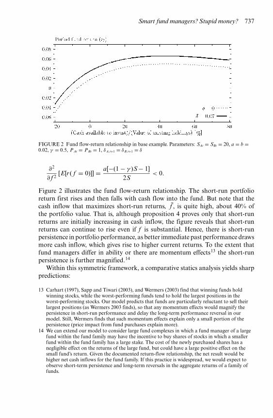
FIGURE 2 Fund flow-return relationship in base example. Parameters: SAt = SBt = 20, a = b =0.02, γ = 0.5, PAt = PBt = 1, δA,t+1 = δB,t+1 = δ

∂2

∂ f 2[E[r ( f = 0)]] = a[−(1 − γ )S − 1]

2S< 0.

Figure 2 illustrates the fund flow-return relationship. The short-run portfolioreturn first rises and then falls with cash flow into the fund. But note that thecash inflow that maximizes short-run returns, f , is quite high, about 40% ofthe portfolio value. That is, although proposition 4 proves only that short-runreturns are initially increasing in cash inflow, the figure reveals that short-runreturns can continue to rise even if f is substantial. Hence, there is short-runpersistence in portfolio performance, as better immediate past performance drawsmore cash inflow, which gives rise to higher current returns. To the extent thatfund managers differ in ability or there are momentum effects13 the short-runpersistence is further magnified.14

Within this symmetric framework, a comparative statics analysis yields sharppredictions:

13 Carhart (1997), Sapp and Tiwari (2003), and Wermers (2003) find that winning funds holdwinning stocks, while the worst-performing funds tend to hold the largest positions in theworst-performing stocks. Our model predicts that funds are particularly reluctant to sell theirlargest positions (as Wermers 2003 finds), so that any momentum effects would magnify thepersistence in short-run performance and delay the long-term performance reversal in ourmodel. Still, Wermers finds that such momentum effects explain only a small portion of thepersistence (price impact from fund purchases explain more).

14 We can extend our model to consider large fund complexes in which a fund manager of a largefund within the fund family may have the incentive to buy shares of stocks in which a smallerfund within the fund family has a large stake. The cost of the newly purchased shares has anegligible effect on the returns of the large fund, but could have a large positive effect on thesmall fund’s return. Given the documented return-flow relationship, the net result would behigher net cash inflows for the fund family. If this practice is widespread, we would expect toobserve short-term persistence and long-term reversals in the aggregate returns of a family offunds.


• Short-run returns fall with the information arrival rate, γ . That is, short-runreturns are higher if information is less likely to leak out by the end of theperiod:

∂ E[r ( f )]∂γ

= −2aI( f )(I( f ) + S)2S + f

< 0.

• Greater cash inflows raise short-run returns by more if information is less likelyto leak out:

∂2 E[r ( f )]∂γ ∂ f

= −(

4aI∂ I( f )

∂ f+ 2aS

∂ I( f )∂ f

)(2S + f )−1

+ 2aI( f )(I( f ) + S)(2S + f )−2

= −2a(2S + f )−2

[I(

2(2S + f )∂ I( f )

∂ f− I( f )

)

+ S(

(2S + f )∂ I( f )

∂ f− I( f )

)]< 0,

because

∂ I( f )∂ f

f > I( f ) and S ≥ 0.

These two predictions can reconcile the finding of Zheng (1999) and othersthat niche mutual funds (which invest in stocks where there are fewer sources ofinformation) have stronger short-run persistence and greater long-run reversalsin performance.

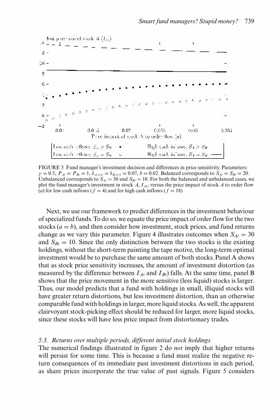
5.2. Differences in price schedulesWe now explore how outcomes are affected if the price impact of trades differsacross stocks. We suppose that �PAt(I At) = aI At and �PBt(I Bt) = bI Bt, wherea = b, but that the stocks are otherwise identical, PAt = PBt = 1 and δAt =δBt = δ. Figure 3 numerically characterizes how I At depends on a when the fundmanager is fully invested. We consider two cases: (i) balanced holdings (SAt =SBt = S); and (ii) unbalanced holdings (SAt > SBt). The figure highlights thatas long as cash inflow, f , is sufficiently small, investment in stock A rises witha; but for higher values of f , investment falls with a. Further, these investmentconsequences are magnified when SAt > SBt. Phrased differently, if and only ifcash inflows are not too high, the gain from strategically manipulating returnsby distorting investments toward greater existing positions rises with the priceimpact of stock A order flow, a. However, if cash inflows are too high, increasesin a reduce investment in stock A, since the strategic manipulation gains aredominated by the increasing marginal cost of additional share purchases.


FIGURE 3 Fund manager’s investment decision and differences in price sensitivity. Parameters:γ = 0.5, PAt = PBt = 1, δA,t+1 = δB,t+1 = 0.07, b = 0.02. Balanced corresponds to SAt = SBt = 20.Unbalanced corresponds to SAt = 30 and SBt = 10. For both the balanced and unbalanced cases, weplot the fund manager’s investment in stock A, I At, versus the price impact of stock A to order flow(a) for low cash inflows ( f = 4) and for high cash inflows ( f = 18)

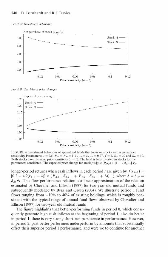
Next, we use our framework to predict differences in the investment behaviourof specialized funds. To do so, we equate the price impact of order flow for the twostocks (a = b), and then consider how investment, stock prices, and fund returnschange as we vary this parameter. Figure 4 illustrates outcomes when SAt = 30and SBt = 10. Since the only distinction between the two stocks is the existingholdings, without the short-term painting the tape motive, the long-term optimalinvestment would be to purchase the same amount of both stocks. Panel A showsthat as stock price sensitivity increases, the amount of investment distortion (asmeasured by the difference between I At and I Bt) falls. At the same time, panel Bshows that the price movement in the more sensitive (less liquid) stocks is larger.Thus, our model predicts that a fund with holdings in small, illiquid stocks willhave greater return distortions, but less investment distortion, than an otherwisecomparable fund with holdings in larger, more liquid stocks. As well, the apparentclairvoyant stock-picking effect should be reduced for larger, more liquid stocks,since these stocks will have less price impact from distortionary trades.

5.3. Returns over multiple periods, different initial stock holdingsThe numerical findings illustrated in figure 2 do not imply that higher returnswill persist for some time. This is because a fund must realize the negative re-turn consequences of its immediate past investment distortions in each period,as share prices incorporate the true value of past signals. Figure 5 considers


FIGURE 4 Investment behaviour of specialized funds that focus on stocks with a given pricesensitivity. Parameters: γ = 0.5, PAt = PBt = 1, δA,t+1 = δB,t+1 = 0.07, f = 4, SAt = 30 and SBt = 10.Both stocks have the same price sensitivity (a = b). The fund is fully invested in stocks for theparameters considered. The expected price change for stock j is [γ a (PjtIjt) + (1 − γ )δ j,t+1] Pjt.

longer-period returns when cash inflows in each period t are given by f (r t−1) =[0.2 + 4.2(r t−1 − δ)] × (PA,t−1SA,t−1 + PB,t−1SB,t−1 + Mt−1), where δ = δAt =δBt ∀t. This flow-performance relation is a linear approximation of the relationestimated by Chevalier and Ellison (1997) for two-year old mutual funds, andsubsequently modelled by Berk and Green (2004). We illustrate period 1 fundflows ranging from −10% to 40% of existing holdings, which is roughly con-sistent with the typical range of annual fund flows observed by Chevalier andEllison (1997) for two-year old mutual funds.

The figure highlights that better-performing funds in period 0, which conse-quently generate high cash inflows at the beginning of period 1, also do betterin period 1: there is very strong short-run persistence in performance. However,in period 2, past better performers underperform by amounts that substantiallyoffset their superior period 1 performance, and were we to continue for another


FIGURE 5 Multi-period example illustrating short-term persistence and long-run reversal ofperformance. Period t cash inflow is calculated as: f t(r t−1) = [0.2 + 4.2 (r t−1 − δ)] × (PA,t−1 SA,t−1 +PB,t−1 SB,t−1 + Mt−1). Period 0 winners are funds for which r 0 > i 0. The y-axis plots mutual fundreturns (r t, t = 1, 2) and the x-axis plots period 1 cash inflows f 1(r 0). Parameters: a = b = 0.02,SA,1 = 30, SB,1 = 10, PA,1 = PB,1 = 1, γ = 0.5; δA,t = δB,t = δ = 0.07 ∀t

period, there would be a long-run reversal in performance. Obviously, if we in-corporated other persistent factors, such as fund manager ability, then long-runreversals would take longer and be less extreme.

According to our flow-performance relation, the initial range of cash inflows(−10% to 40%) implies a difference in period 0 returns of 0.3% to 30.0%. Thisdispersion of returns is much larger than the dispersion of observed period 1 re-turns obtained using our model: 5.7% to 12.5%. This suggests that, while paintingthe tape drives short-run persistence and long-run reversal patterns, other exoge-nous factors such as idiosyncratic stochastic shocks drive much of the dispersionin observed returns. In particular, this confirms that taking r0 and hence initialcash flows as exogenous (as we do in our propositions) is unimportant, as ourqualitative findings would extend.15

There is significant anecdotal and empirical evidence that suggests funds con-duct much of their trade near the end of a quarter. In addition to the trad-ing behaviour that we model, there is evidence of ‘window dressing’ (selling thefund’s lacklustre holdings before they are revealed to investors in end-of-quarterreports). If selling poorly performing stock holdings near the end of quarters isprevalent, then fund managers will have more cash on hand than normal to makenew investments near the end of quarters. Our model predicts that fund managerswill tend to use this cash to buy shares that magnify the value of the fund’s ex-isting holdings (i.e., stocks in which the fund has many shares or stocks that are

15 In unreported results, we confirmed that our qualitative findings are not affected by startingvalues by iterating our model over an arbitrary number of periods and verifying that the sameshort-run persistence and long-run reversal patterns exist in later periods.


thinly traded). This behaviour has very different implications for mutual fundreturn patterns than the window-dressing motive of buying winners (in whicha fund may or may not have a substantial existing position). Window dressingalone cannot generate the short-run persistence and long-run reversal patternsin the data.16

6. Conclusion

This paper provides a theoretical framework for understanding the incentives for,and the implications of, mutual fund managers distorting end-of-quarter stockpurchases toward stocks in which the fund has larger existing positions. We showhow this common practice, sometimes known as painting the tape, depends on theshort-term price impact of trades and the relation between past fund performanceand future fund cash inflows.

We derive when and how such trading leads to the empirically observed short-run persistence and long-run reversal in fund performance. Our model also ex-plains why mutual funds tend to be relatively undiversified and exhibit persistentstock selection. Our theoretical predictions are consistent with the empirical find-ings of Carhart et al. (2002) that trading-induced equity price inflation on the lastday of a quarter gives rise to abnormal fund returns on those days and that the endof year performance effect is more pronounced for better historical performers.

Our unified framework for analyzing mutual fund investment distortion pro-vides several directions for future empirical research. For instance, fund managerswill invest more heavily on the basis of private information earlier in an evaluationperiod and this should be reflected in the long-run return characteristics of thesepurchases. As well, the short-run persistence, long-run reversal pattern should beexhibited only by funds that are effectively fully invested in the market (excludingcash held for insurance against unexpected redemptions). And funds with a moresensitive performance-flow relation should exhibit greater investment distortion.Finally, we argue that existing measures of mutual fund managers’ true stockpicking ability have been understated because of their failure to recognize theadditional costs of the strategic behaviour modelled in our paper.

Appendix A: Proofs

We note that maximizing portfolio returns also maximizes the portfolio end-of-period value. Thus, the Lagrangian corresponding to the manager’s problem is

16 So, too, Carhart et al. (2002) find that mutual fund net asset value inflation in excess of the S&P500 index on the last day of a quarter is at least 0.2% to 0.4% for funds in lesser deciles. Carhartet al. argue that this is caused by a ‘leaning-for-the-tape’ motive, in which fund managers nearthe top of the return rankings have the most to gain from performance rank improvements(consistent with the empirical findings of Ippolito 1992 and Sirri and Tufano 1998) and thushave the most to gain from end-of-quarter distortionary trades. But this leaning-for-the-tapemotive alone cannot generate short-term persistence in mutual fund returns because there is nolink between past- and current-period fund performance.


L(Mt, IAt, IBt) = Mt +∑

j

(Ijt + Sjt)E[P∗

j t

] + λMMt + λA[SAt + IAt

]

+ λB[SBt + IBt

] + λbud[

f (rt−1) + Mt−1 − [PAt

+ �PAt(PAt, IAt)]IAt − [PBt + �PBt(PBt, IBt)]IBt − Mt].

Given that λM = λA = λB = 0, the associated first-order condition characterizingthe optimal investment in stock j ∈ {A, B} is

∂L∂ Ijt

= Pjt + (1 − γ )�Pjt(Pjt, Ijt) + γ δPjt + (1 − γ )Ijt∂�Pjt

∂ Ijt

+ (1 − γ )Sjt∂�Pjt

∂ Ijt− λbud

[Pjt + �P(Pjt, Ijt) + Ijt

∂�Pjt

∂ Ijt

]= 0.

Proof of proposition 1. From the first-order conditions:

λbud =PAt + (1 − γ )�P(PAt, IAt) + γ δ1 PAt + (1 − γ )(IAt + SAt)

∂�P∂ IAt

PAt + �P(PAt, IAt) + IAt∂�P∂ IAt

(8)

=PBt + (1 − γ )�P(PBt, IBt) + γ δ2 PBt + (1 − γ )(IBt + SBt)

∂�P∂ IBt

PBt + �P(PBt, IBt) + IBt∂�P∂ IBt

. (9)

Substituting for �P(Pj, I j) = k (PjIj) Pj,

(1 − γ ) + γ + γ δ1 + PAt SAt(1 − γ )k1 + 2kPAt IAt

= (1 − γ ) + γ + γ δ2 + PBt SBt(1 − γ )k1 + 2kPBt IBt

.

(10)

Then, reversing PAtSAt and PBtSBt, holding PAtIAt and PBtIBt fixed, it is clear that

γ + γ δ1 + PBt SBt(1 − γ )k1 + 2kPAt IAt

<γ + γ δ2 + PAt SAt(1 − γ )k

1 + 2kPBt IBt.

To restore equality, it follows that the optimal values of I At and I Bt must satisfyPAtIAt(δ1, δ2) > PBtIBt(δ2, δ1). Then it follows that

(PAt + �P(PAt, IAt(δ1, δ2)))IAt(δ1, δ2)

> (PBt + �P(PBt, IBt(δ2, δ1)))IBt(δ2, δ1). �

Proof of proposition 2. Re-arranging (10) gives

γ (1 + δA − kPASA) + kPASA

γ (1 + δB − kPBSB) + kPBSB= 1 + 2kPAt IAt

1 + 2kPBt IBt. (11)


Taking the derivative of the left-hand side of (11) with respect to γ gives

k(PBSB − PASA) + δAPBSBk − δB PASAk

[γ (1 + δB − kPBSB) + kPBSB]2.

Since PASA > PBSB, this derivative is negative if δA ≤ δB or more generally iffcondition (7) holds. Since the right-hand side of (11) is increasing in PAtIAt, ourdesired result follows directly. �

Proof of proposition 3. If Mt > 0, then λbud = 1 and the marginal dollar is investedin cash (dMt/d f = 1; ∂ Ijt/d f = 0, j = A, B). Differentiating short-run expectedreturns,

E[rt] = [Mt + E[P∗

At](IAt + SAt) + E[P∗Bt](IBt + SBt)

]× [

PAt SAt + PBt SBt + f (rt−1)]−1 − 1,

with respect to f = f (r t−1) at the manager’s optimal values of I At and I Bt yields

∂ E[rt(IAt, IBt)]∂ f

=[

d Mt

d f+ d

d f

{E[P∗

At](IAt + SAt) + E[P∗Bt](IBt + SBt)

}]

× [PAt SAt + PBt SBt + f ]−1 − [Mt + E[P∗At](IAt + SAt)

+E[P∗Bt](IBt + SBt)][PAt SAt + PBt SBt + f ]−2

= [PAt SAt + PBt SBt + f ]−1 − [Mt + E[P∗At](IAt + SAt)

+ E[P∗Bt](IBt + SBt)][PAt SAt + PBt SBt + f ]−2

= −E[rt][PAt SAt + PBt SBt + f ]−1 ≤ 0,

if E[rt] ≥ 0; strict if E[rt] > 0,

where the last equality follows from substitution. �

Proof of proposition 4. From the budget constraint,

f = [PAt + �PAt(PAt, IAt)]IAt + [PBt + �PBt(PBt, IBt)]IBt (12)

1 = ∂ IAt

∂ f(PAt + �PAt) + ∂�PAt

∂ IAt

∂ IAt

∂ fIAt + ∂ IBt

∂ f(PBt + �PBt)

+ ∂�PBt

∂ IBt

∂ IBt

∂ fIBt.

We first prove the result that short-run returns are increasing in f when I At andI Bt are small if f is close to zero (as will be the case for SAt ∼ SBt, and PAt ∼ PBt).


Then, it follows that

1 = ∂ IAt

∂ fPAt + ∂ IBt

∂ fPBt.

If the fund manager is fully invested, then expected returns are

E[rt] =∑j={A,B}

{(1 + γ δ)Pjt(Ijt + Sjt) + (1 − γ )�Pjt(Pjt, Ijt)(Ijt + Sjt)

}

PAt SAt + PBt SBt + f− 1.

(13)

Thus,

∂ E[rt]∂ f

∣∣∣∣f =0

= [PAt SAt + PBt SBt]−1

[(1 − γ )

(∂�PAt

∂ IAt

∂ IAt

∂ fSAt

+ ∂�PBt

∂ IBt

∂ IBt

∂ fSBt

)+ (1 + γ δ)

(∂ IAt

∂ fPAt + ∂ IBt

∂ fPBt

) ]

−[

(1 + γ δ)(PAt SAt + PBt SBt)(PAt SAt + PBt SBt)2

].

(14)

Substituting for PBt(∂ I Bt/∂ f ) + PAt(∂ I At/∂ f ) = 1 yields

∂ E[rt]∂ f

∣∣∣∣f =0

= [PAt SAt + PBt SBt]−1(1 − γ )[∂�PAt

∂ IAt

∂ IAt

∂ fSAt

+ ∂�PBt

∂ IBt

∂ IBt

∂ fSBt

]> 0, (15)

since ∂�Pkt/∂ I k > 0 (by assumption) and ∂ I kt/∂ f > 0 (since (10) can hold onlyif an increase in I At coincides with an increase in I Bt).

More generally to show that the derivative of returns with respect to f ispositive recognize that this amounts to showing that

sign[(PAt SAt + PBt SBt)

∂num∂ f

− num]

| f =0> 0,

where num is the numerator of expected returns. Equivalently, dividing throughby PAtSAt + PBtSBt, it amounts to showing that

sign[∂num∂ f

− (1 + E[rt])]

| f =0

= sign[λbud − (1 + E[rt])

]| f =0

> 0,

where the equality follows from substitution of equations (8) and (9). That is,λbud reflects the marginal return of one more dollar, and if the marginal return


exceeds 1 + r t, then r t must be increasing in f . The Lagrange multiplier can beinterpreted as the marginal value of one more dollar of investment in stock A oras the reduction in the marginal cost of selling one more dollar of investment instock B. We now show that for δ ≥ 0, this marginal cost grows monotonically asthe fund manager sells more I B. Differentiating (9) with respect to I Bt, we seethat it has sign

(PBt + �P(PBt, IBt) + IBt�P′(PBt, IBt))

× [(1 − γ )(2�P′(PBt, IBt) + IBt�P′′(PBt, IBt)) + SBt(1 − γ )�P′′(PBt, IBt)]

−(2�P′(PBt, IBt) + IBt�P′′(PBt, IBt))

× [PBt + (1 − γ )�P(PBt, IBt) + γ δPBt + (1 − γ )(IBt + SBt)�P′(PBt, IBt)]

< (PBt + �P(PBt, IBt) + IBt�P′(PBt, IBt))SBt(1 − γ )�P′′(PBt, IBt)]

− (2�P′(PBt, IBt) + IBt�P′′(PBt, IBt))(γ δPBt + SBt(1 − γ )�P′(PBt, IBt))]

< 0,

where the last inequality follows from δ ≥ 0 and A4. λbud takes its value evaluatedat I∗

Bt, so that it exceeds the derivative evaluated at I Bt = 0, which we have provenexceeds r t. For δ < 0 an analogous exercise on (8) establishes monotonicity forI At > 0.

Finally, short-run returns must eventually decline with f : A4 implies thatmarginal returns from making arbitrarily large purchases of a stock musteventually become negative. This implies that once f grows sufficiently large,the fund manager begins to invest in cash at the point where the marginalreturn on investing in stock is i (which we normalized to zero), and where theshort-run portfolio return exceeds i. It follows that for f larger, short-run returnsdecline. �

References

Alexander, G.J., G. Cici, and S. Gibson (2007) ‘Does motivation matter when assessingtrade performance? An analysis of mutual funds,’ Review of Financial Studies 20, 125–50

Baks, K.P. (2007) ‘On the performance of mutual fund managers,’ Journal of Finance,forthcoming

Berk, J.B., and R.C. Green (2004) ‘Mutual fund flows and performance in rational mar-kets,’ Journal of Political Economy 112, 1269–95

Bernhardt, D., and R.J. Davies (2005) ‘Painting the tape: aggregate evidence,’ EconomicsLetters 89, 306–11

Bernhardt, D., and E. Nosal (2008) ‘Gambling for dollars: a strategic analysis of hedgefunds,’ working paper, University of Illinois

Bernhardt, D., and B. Taub (2008) ‘Cross-asset speculation in stock markets,’ Journal ofFinance, forthcoming

Bhattacharyya, S., and V. Nanda (2007) ‘Portfolio pumping, trading activity, and fundperformance,’ working paper, University of Michigan


Bollen, N.P.B., and J.A. Busse (2005) ‘Short-term persistence in mutual fund performance,’Review of Financial Studies 18, 569–97

Brown, S.J., and W.N. Goetzmann (1995) ‘Performance persistence,’ Journal of Finance50, 679–98

Caballe, J., and M. Krishnan (1994) ‘Imperfect competition in a multi-security marketwith risk neutrality,’ Econometrica 62, 695–704

Carhart, M.M. (1997) ‘On persistence in mutual fund performance,’ Journal of Finance52, 57–92

Carhart, M.M., R. Kaniel, D.K. Musto, and A.V. Reed (2002) ‘Leaning for the tape:evidence of gaming behavior in equity mutual funds,’ Journal of Finance 57, 661–93

Chan, L.K.C., and J. Lakonishok (1995) ‘The behavior of stock prices around institutionaltrades,’ Journal of Finance 50, 1147–74

Chevalier, J., and G. Ellison (1997) ‘Risk taking by mutual funds as a response to incen-tives,’ Journal of Political Economy 105, 1167–200

Edelen, R. (1999) ‘Investor flows and the assessed performance of open-end mutual funds,’Journal Financial Economics 53, 439–66

Gallagher, D.R., P. Gardner, and P.L. Swan (2007) ‘Portfolio pumping: an examination ofinvestment manager quarter-end trading and impact on performance,’ working paper,University of New South Wales

Gruber, M.J. (1996) ‘Another puzzle: the growth in actively managed mutual funds,’Journal of Finance 51, 783–810

Hendershott, T., and M. Seasholes (2007) ‘Market maker inventories and stock prices,’American Economic Review (Papers and Proceedings) 97, 210–14

Hendricks, D., J. Patel, and R. Zeckhauser (1993) ‘Hot hands in mutual funds: short-runpersistence of relative performance, 1974–1988,’ Journal of Finance 48, 93–130

Hu, F., A. Hall, and C.R. Harvey (2000) ‘Promotion or Demotion? An empirical investi-gation of the determinants of top mutual fund manager change,’ working paper, DukeUniversity

Hugonnier, J., and R. Kaniel (2008) ‘Mutual fund portfolio choice in the presence ofdynamic flows,’ Mathematical Finance, forthcoming

Ippolito, R. (1992) ‘Consumer reaction to measures of poor quality: evidence from themutual fund industry,’ Journal of Law and Economics 35, 45–70

Kacperczyk, M., C. Sialm, and L. Zheng (2005) ‘On the industry concentration of activelymanaged equity mutual funds,’ Journal of Finance 60, 1983–2011

Keim, D.B., and A.N. Madhavan (1996) ‘The upstairs market for large-block transactions:analysis and measurement of price effects,’ Review of Financial Studies 9, 1–36

— (1997) ‘Transaction costs and investment style: an inter-exchange analysis of institu-tional equity trades,’ Journal of Financial Economics 46, 265–92

Kyle, A. (1985) ‘Continuous auctions and insider trading,’ Econometrica 53, 1315–35Malkiel, B.G. (1995) ‘Returns from investing in equity mutual funds, 1971 to 1991,’ Journal

of Finance 50, 549–72Pinnuck, M. (2003) ‘An examination of the performance of the trades and stockholdings

of fund managers: further evidence,’ Journal of Financial and Quantitative Analysis 38,811–28

San, G. (2007) ‘Who gains more by trading – institutions or individuals?’ Working paper,Hebrew University of Jerusalem

Sapp, T.R.A., and A. Tiwari (2004) ‘Does stock return momentum explain the ‘smartmoney’ Effect?’ Journal of Finance 59, 2605–22

Sirri, E.R., and P. Tufano (1998) ‘Costly search and mutual fund flows,’ Journal of Finance53, 1589–622

Wermers, R. (2003) ‘Is money really ‘‘smart’’? New evidence on the relation betweenmutual fund flows, manager behavior, and performance persistence,’ working paper,University of Maryland


Wermers, R., L. Chen, and N. Jegadeesh (2000) ‘The value of active mutual fund man-agement: an examination of the stockholdings and trades of fund managers,’ Journalof Financial and Quantitative Analysis 35, 343–68

Yan, X. (2006) ‘The determinants and implications of mutual fund cash holdings: theoryand evidence,’ Financial Management 35, 69–91

Zheng, L. (1999) ‘Is money smart? A study of mutual fund investors’ fund selection ability,’Journal of Finance 54, 901–33

Economy & Finance

Smart fundmgrsstupidmoney bernhardt