Should robots be taxed?

1/56

Should Robots Be Taxed?

Joao Guerreiro, Sergio Rebelo, and Pedro Teles

November 2017

Should Robots Be Taxed? Joao Guerreiro, Sergio Rebelo, and Pedro Teles

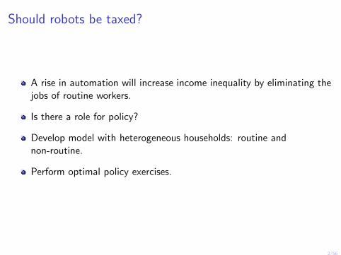
Should robots be taxed?

A rise in automation will increase income inequality by eliminating thejobs of routine workers.

Is there a role for policy?

Develop model with heterogeneous households: routine andnon-routine.

Perform optimal policy exercises.

2/56

Outline

1. Model of automationI Static model. Dynamic considerations discussed at the end

2. Equilibrium with current tax system (status-quo equilibrium)

3. First-best solution

4. Mirrleesian second-best solution

5. Optimal policy with simple income taxes

6. Welfare comparison

7. Endogenous occupational choice

8. Relation to public finance literature

9. Conclusion

3/56

4/56

Model


Model of automation

Two representative households,

I One with routine workers, j = r ,I The other with non-routine workers, j = n.

PreferencesUj = u(Cj)− v(Nj) + g(G ),

Cj = consumption, Nj = hours worked, G = government spending.

Budget constraintCj ≤ wjNj − T (wjNj),

wj =wage rate worker type j ,

T (·) = income tax schedule.

5/56

Robot producers

Robots are an intermediate input. Final good producers can userobots in tasks i ∈ [0, 1].

Robots for each task i are produced by competitive firms.

Cost of producing a robot φ units of output. Identical across tasks.

Problem of firm that produces robots to automate task i is

πi = maxxi

pixi − φxi .

It follows thatpi = φ.

6/56

Final good producers

A representative firm hires non-routine labor (Nn).

For each task i , hire routine labor (ni ) or buy intermediate goods (xi )which we refer to as robots.

Production function:

Y = A

[∫ m

0xρi di +

∫ 1

mnρi di

] 1−αρ

Nαn ,

I CES aggregator for tasks and Cobb-Douglas in tasks and non-routinelabor.

I Each task may be produced by robots or routine workers (perfectsubstitution).

I Since tasks are symmetric, assume first m are automated, and last(1−m) use routine workers.

7/56


Representative firm problem is to choose xi , ni ,m,Nn to maximize

π = Y − wnNn − wr

∫ 1

mnidi −

∫ m

0(1 + τx)φxidi .

τx = linear tax on robots.

8/56


xi = x constant in [0,m].

ni = n constant in (m, 1].

If wr = (1 + τx)φ, there’s partial automation (m ∈ [0, 1]).

With partial automation the levels of routine labor and robots are thesame: x = n.

9/56

Government

Government choosesI Income taxation, T (·).I Tax on robots, τx .I Government spending, G .

Budget constraint:

G ≤ T (wrNr ) + T (wnNn) +

∫ m

0τxφxidi .

I Tax schedule is the same for both types of workers.

10/56

Market clearing

Routine labor: ∫ 1

mnidi = Nr .

Output market:

Cr + Cn + G ≤ A

[∫ m

0xρi di +

∫ 1

mnρi di

] 1−αρ

Nαn −

∫ m

0φxidi .

I Cost of robot production subtracted from final output.

11/56

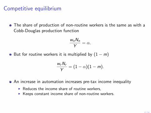
Competitive equilibrium

The share of production of non-routine workers is the same as with aCobb-Douglas production function

wnNn

Y= α.

But for routine workers it is multiplied by (1−m)

wrNr

Y= (1− α)(1−m).

An increase in automation increases pre-tax income inequality

I Reduces the income share of routine workers,I Keeps constant income share of non-routine workers.

12/56

With partial automation

With partial automation, total routine labor supplied is split equallyby 1−m non-automated tasks:

ni =Nr

1−m, for i ∈ (m, 1] ,

Robots in the first m tasks are used at the same level.

Equilibrium level of automation is

m = 1−[

(1 + τx)φ

(1− α)A

]1/α Nr

Nn.

13/56

With partial automation

Wage rates are given by technological parameters (independent ofpreferences)

wn = αA1/α(1− α)

1−αα

[(1 + τx)φ]1−αα

,

wr = (1 + τx)φ.

I Tax on robots increases wage of routine, but decreases wage ofnon-routine.

I In that way, this instrument affects the relative wage.

14/56

15/56

Status-quo equilibrium



Heathcote, Storesletten and Violante (2014) propose after-tax incomefunction

y(wjNj) = λ(wjNj)1−γ ,

T (wjNj) = wjNj − λ(wjNj)1−γ .

λ controls the level of taxation (higher λ implies lower average taxes).

γ controls the progressivity of the tax code (γ > 0 impliesprogressivity).

HSV estimates using PSID data

I γ = 0.185 (income taxes close to linear),I R2 is 0.92.

16/56


Functional form for utility function:

I Uj = log(Cj) + θ log(1− Nj) + χ log(G ).I θ = 1.63, which implies Nj = 1/3.I χ = 0.25.

Policy:I Government sets its spending to 20 percent of outputI Sets γ = 0.185 and adjusts λ to balance budgetI Robots are not taxed, τx = 0.

Production parameters:

I A = 1, α = 0.5 (symmetry).

17/56


I Only non-routine workers benefit from automation.I Consumption of routine workers goes to zero.I Full automation never occurs.

18/56

19/56

First-best allocation



Planner maximizes average utility

V =1

2Ur +

1

2Un,

I Possible interpretation: ex-ante, workers do not know whether they areroutine or non-routine, planner maximizes expected utility.

subject to resource constraints

Cr + Cn + G ≤ Y − φ∫ m

0xidi ,

Y = A

[∫ m

0xρi di +

∫ 1

mnρi di

] 1−αρ

Nαn ,∫ 1

mnidi = Nr .

20/56


Agents have equal consumption in the first best.

More productive agents work more.

⇒ When types are not observable, this allocation cannot beimplemented

I High productivity agents would pretend to be low productivity.

21/56


I Routine workers have higher utility than non-routine.I Routine workers always benefit from automation.I Non-routine workers eventually benefit.

22/56


While interesting as a benchmark, the first best is not implementablewhen there are restrictions on the tax system.

For that reason we will turn to plans that satisfy restrictions:

I Informational restrictions, in the spirit of Mirrlees (1971);

I Instrument restrictions, in the tradition of Ramsey (1927).

23/56

24/56

Mirrleesian optimal taxation



Government does not observe agent’s type or labor supply.

Government observes an agent’s total income. Incentive compatibleincome taxation.

Robot taxes are assumed to be proportional, τx .

I Guesnerie (1995): non-linear taxes on intermediate inputs createarbitrage opportunities. Difficult to implement.

25/56


In Mirrlees (1971) differences in agents’ productivities are exogenous.

In our model, productivity differences are endogenous and depend onτx .

Key question: is it optimal to distort production decisions by taxingthe use of robots to redistribute income from non-routine to routineworkers to increase social welfare?

26/56


Planner’s problem:

W (τx) = max1

2[u(Cr )− v (Nr ) + g(G )]

+1

2[u(Cn)− v (Nn) + g(G )] ,

subject to resource constraint

Cr + Cn + G ≤ wnNnτx + α

α(1 + τx)+

wrNr

1 + τx.

and two incentive compatibility (IC) constraints

u(Cn)− v (Nn) ≥ u(Cr )− v (wrNr/wn) ,

u(Cr )− v (Nr ) ≥ u(Cn)− v (wnNn/wr ) .

Optimal choice of τx requires W ′(τx) = 0.

27/56


Proposition

In the optimal plan, when automation is incomplete (m < 1) robot taxesare strictly positive (τx > 0).

Increasing τx generates a first-order gain from loosening theinformational restriction of the non-routine worker:

u(Cn)− v(Nn) ≥ u(Cr )− v

(wr

wnNr

).

If τx < 0, a marginal increase in τx is also in the direction ofproduction efficiency.

If τx = 0, a marginal increase in τx induces output losses, but onlysecond order.

A planner that chooses τx ≤ 0 can always improve its objective with amarginal increase in τx .

28/56

Mirrleesian optimal taxation - with full automation

With full automation, Yr = 0 and m = 1, the IC of the non-routineworker becomes

u(cn)− v(nn) = u(cr )

Robot taxes no longer affect this constraint.

Routine and non-routine workers have the same utility.

29/56


I Modest levels of robot taxes. These become zero once routine workersare replaced by robots.

I With full automation agents have the same utility. Planner cannotfurther transfer towards routine workers.

30/56

31/56

Simple income tax systems


Simple taxes

The Mirrleesian plan may be a big deviation from the income taxsystems that we observe in actual economies.

How close to the Mirrleesian second best can an empirically plausibletax function take us?

Is there a simple modification of such tax system that would generatea large improvement?

⇒ Restrictions on instruments - Ramsey tradition

32/56

Simple taxes

Optimal tax policy when the tax schedule has form proposed byHeathcote, Storesletten and Violante (2014)

T (wjNj) = wjNj − λ(wjNj)1−γ ,

With this formulation the ratio of consumptions is

Cr

Cn=

[(1− α)(1−m)

α

]1−γ.

Two ways to make ratio Cr/Cn closer to one.

I Raise τx which leads to a fall in the level of automation, m.

F Reduces production efficiency.

I Make γ closer to one, i.e. make the tax system more progressive.

F Reduces incentives to work.

33/56

Simple taxes

Cr

Cn=

[(1− α)(1−m)

α

]1−γ.

The planner will balance making the system more progressive anddistorting m downwards.

Full automation is never optimal.I That would lead the routine worker to consume zero.

34/56

Simple taxes

I High taxes on robots = high production distortions.I Both agents eventually benefit from automation.I Full automation never occurs.

35/56

Simple taxes

36/56

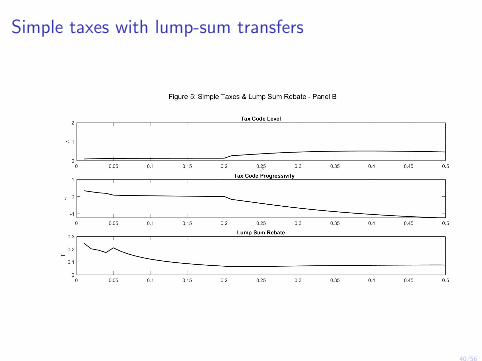
Simple taxes with lump-sum transfers

The previous tax system leads to very high taxation of robots, largeproduction inneficiency.

Simple modification: allow for lump-sum rebates, Ω.

T (wjNj) = wjNj − λ(wjNj)1−γ − Ω.

In this case, the ratio of consumptions is given by

Cr

Cn=

[(1− α)(1−m)]1−γ + ω

α1−γ + ω,

ω =Ω

λY 1−γ .

37/56


Cr

Cn=

[(1− α)(1−m)]1−γ + ω

α1−γ + ω.

Lump-sum rebate helps redistributing income

Agents receive income even if they do not work

⇒ Full automation is possible.

38/56


I Full automation is recovered.I Robot taxes are zero after full automation (since Nr = 0 robot taxes do

not help redistribution).I The utility of routine gets closer to non-routine.

39/56


40/56

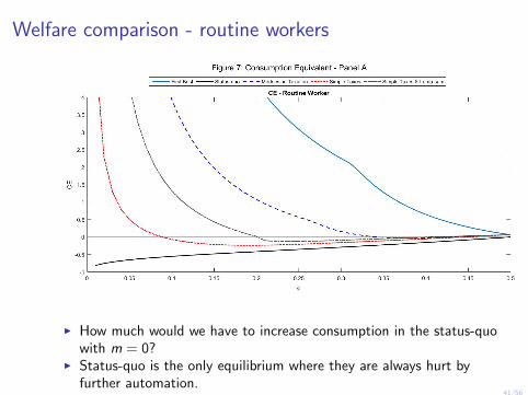
Welfare comparison - routine workers

I How much would we have to increase consumption in the status-quowith m = 0?

I Status-quo is the only equilibrium where they are always hurt byfurther automation.

41/56

Welfare comparison - non-routine workers

I Best equilibrium is status-quo, they are the only ones to benefit fromdecreasing automation costs.

I Apart from first best they are always better off by further automation.I First-best planner can induce non-routine to work more, and

temporarily lose with automation.42/56

43/56

Endogenous occupational choice



Suppose now that agents can move between occupations.

Household type θ has preferences over the two occupations.

u(Cθ)− v(Nθ) + g(G )−Oθθ.

Oθ = 1 if household becomes non-routine, and Oθ = 0 otherwise.

I If θ < 0 the household prefers non-routine occupations.

I If θ > 0 the household prefers routine occupations.

The agent receives the wage wn if he decides to become non-routineand wr if he decides to become routine.

44/56


Agents choose both their occupation and the number hours worked.

There are two incentive constraints:

I Intensive margin - labor supply IC

u(Cθ)− v(Nθ) ≥ u(Cθ′)− v(wθ′

wθNθ′

).

I Extensive margin - occupation choice IC

u(Cθ)− v(Nθ)−Oθθ ≥ u(Cθ′)− v(Nθ′)−Oθ′θ.

45/56


In the optimum, agents that choose the same occupation have thesame levels of consumption and hours of work.

The extensive margin incentive compatibility is summarized by athreshold rule

θ∗ = [u(Cn)− v(Nn)]− [u(Cr )− v(Nr )].

I Agents with θ > θ∗ choose to be routine workers.I Agents with θ ≤ θ∗ become non-routine.

46/56


We assume that θ is drawn from a normal distribution with mean zeroand standard deviation σ.

Half of the population prefers non-routine work.

The other half prefers routine work.

47/56

Endogenous occupational choice - First best

I For lower σ: more agents become non-routine.I For lower σ: everyone works less and has higher consumption.

48/56

Endogenous occupational choice - Mirrlees Optimal Taxes

I When occupation switching costs are lower: redistribute by inducingmore agents to become non-routine.

I There is less of a need to resort to robot taxes.I Worse deal for the remaining routine.

49/56

Endogenous occupational choice - Mirrlees Optimal Taxes

I With σ = 1, redistribution by moving agents to non-routine ⇒ Morenon-routine than in first best.

I With σ = 2, direct redistribution and more robot taxes ⇒ Lessnon-routine than in first best.

50/56

51/56

Back to taxation of intermediategoods


Back to taxation of intermediate goods

Diamond & Mirrlees (1971)

I Assumes that government can tax different goods at different rates.I In our model this assumption would allow taxing routine and

non-routine workers at different rates.I When direct tax discrimination is not possible, robots will be taxed

provided this helps treating different agents differently.

Atkinson & Stiglitz (1976)

I Assumes that labor types are perfect substitutes.I This implies that intermediate goods do not interact differently with

different labor types.I These assumptions do not hold in our model.

F Robots are substitutes for routine workers and complements fornon-routine workers.

52/56

Robots as capital

Robots are durable goods.

Taxing robots creates intertemporal distortions, in addition toproduction inneficiency.

Intertemporal distortions might be optimal for reasons orthogonal tothe ones studied in this paper:

I To confiscate the initial stock, if the set of tax instruments is limited.I Because the elasticities of the marginal utility of consumption and

labor are time varying.I With idiosyncratic risks, there may be insurance motives.

As a capital good, robots would be taxed by a capital income taxwithout full deduction of investment.

I South Korea will limit tax incentives for investment in automatedmachines, as part of a revision of tax laws. Effective begining of 2018.

53/56

Conclusions

With current U.S. tax system, a sizable fall in automation costs leadsto large rise in income inequality.

I Routine-worker wages fall to make them competitive with automation.

I Only non-routine workers benefit from advances in automation.

I Full automation never occurs: routine workers always supply labor astheir income and consumption approach zero.

Inequality can be reduced by raising marginal tax rates paid byhigh-income individuals and by taxing robots to raise the wages ofroutine workers.

I Eventually both agents benefit from advances in automation.

I Full automation never occurs.

I This solution involves a substantial efficiency loss.

54/56

Conclusions

Mirrleesian optimal income tax can reduce inequality at a smallerefficiency cost.

I Lower taxes on robots.

I Full automation occurs for relatively high automation costs.

I However, this tax system can be complex and difficult to implement.

Simpler approach with large gains: amend tax system to includelump-sum rebates.

I Solution get closer to Mirrleesian solution.

I When costs of automation are sufficiently low, routine workers stopworking and live off transfers.

55/56

Conclusions

With endogenous occupational choice:

I The planner can switch agents between occupation to redistribute.I For lower switching costs:

F More agents change to non-routine occupations

F There is less of a role for robot taxes.

56/56

Economy & Finance

Should robots be taxed?