BACHELOR THESIS

KEY DETERMINANTS OF THE

SHADOW BANKING SYSTEM THE CASES OF EURO AREA, UNITED KINGDOM AND

UNITED STATES.

Author: Álvaro Álvarez-Campana Rodríguez

Tutor: David Martínez-Miera

Bachelor: Business Administration

Madrid, June 2016

2

ABSTRACT

This paper presents two models of key determinants in the evolution of the shadow

banking system. First of all, a shadow banking measure is built from a European

perspective. Secondly, information on several variables is retrieved basing their selection

in previous literature. Thirdly, those variables are grouped in: 1) the base model: real

GDP, Institutional investors’ assets, term-spread, banks’ net interest margin and liquidity;

and 2) the extended model: the former five plus an indicator of systemic stress, an index

of banking concentration and inflation. Finally, regression analysis on those models is

conducted for different countries’ samples. Both OLS and panel data analysis is

undergone. Results suggest important and consistent geographical differences in relations

between shadow banking and key determinant variables’ effects. Thus, this essay

provides financial authorities with a valuable benchmark to which they should pay

attention before designing optimal policies seeking to reduce the financial risk that

shadow banking entails.

Keywords: shadow banking, financial stability, banking crisis, great recession, key

determinants.

JEL Classification: G21, G23

I am very grateful to David Martinez-Miera for his guidance and advice, Silvia Mayoral Blaya

for her assistance, and Mar García, Irene Rodríguez, Jesús Álvarez-Campana and Pablo Álvarez-

Campana for their inestimable support.

3

Table of contents.

ABSTRACT ...................................................................................................................................... 2

I. INTRODUCTION ..................................................................................................................... 4

I.1 Why is Shadow Banking System so relevant? ...................................................................... 4

I.2 What is this paper’s contribution? ....................................................................................... 5

II. WHAT IS SHADOW BANKING? ............................................................................................... 7

III. LITERATURE REVIEW. .......................................................................................................... 11

III.1 First research on SBS. ....................................................................................................... 11

III.2 SBS definition. .................................................................................................................. 11

III.3 SBS measure. .................................................................................................................... 13

III.4 SBS determinants. ............................................................................................................ 15

III.5 Latest research on SBS. .................................................................................................... 16

IV. DATA AND METHODOLOGY ............................................................................................... 18

IV.1 Framework. ...................................................................................................................... 18

IV.2 Data description. .............................................................................................................. 19

IV.3 Models and extensions. ................................................................................................... 24

IV.4 Limitations ........................................................................................................................ 26

V. RESULTS .............................................................................................................................. 28

V.1 Cross-sectional data approach. ......................................................................................... 28

V.1.1 Whole-sample base and extended model analysis. ................................................... 28

V.1.2 Core base model analysis. .......................................................................................... 29

V.2 Panel data approach. ........................................................................................................ 30

V.2.1 Whole-sample base and extended model analysis. ................................................... 30

V.2.2 Core base model analysis ........................................................................................... 31

V.2.3 Core extended model analysis. .................................................................................. 34

VI. CONCLUSIONS ................................................................................................................... 36

REFERENCES ................................................................................................................................ 38

ABBREVIATIONS .......................................................................................................................... 41

APPENDICES ................................................................................................................................ 42

4

I. INTRODUCTION

I.1 Why is Shadow Banking System so relevant?

After the recent global financial crisis, authorities are concerned about the role that the

shadow banking plays in promoting the risk build up in the financial system. This process

of increasing the risk hinders financial stability, and it could facilitate the appearance of

spill-overs to other macroeconomic sectors. This worry within the international financial

institutions can be seen in some papers published by the European Central Bank (ECB),

the International Monetary Fund (IMF), or even the Federal Reserve Bank (FRB).

One of the most relevant claims of the ECB is that the interconnections between the

regulated and the non-regulated segments of the financial sector have increased.

Moreover, Basel III Accords on stringing capital and liquidity requirements for credit

institutions, would provide the former with more incentives to shift their financial

activities into the hardly regulated shadow banking system (SBS).1 According to this vein,

the Managing Director of the IMF, Christine Lagarde, shows her concern about the rapid

escalation of the less-regulated nonbank sector. She also states the necessity to unveil the

real functioning of this part of the financial system hidden in the shadows. However, she

mentioned the importance of SBS in the process of financing the economy which can

complement positively the traditional system.2

Credit intermediation has always existed outside the regulated banking system. The recent

rise of the concerns and the interest in sizing and understanding the shadow banking

system is closely related to the 2008 worldwide financial crisis (“great recession”). The

housing boom in the United States in early 2000s was mainly financed through the

originate-to-distribute model of banking. In this particular case, the majority of

securitization was made through asset-backed securities (ABS3), and more precisely,

through a special type of ABS called mortgage backed securities (MBS4) serving as

collateral.5 These securities’ usage as collateral was pretty new at that moment. It was

1 See Bakk-Simon et al. (2012). 2 See Lagarde (2014). 3 Deutsche Bundesbank defines an asset-backed security (ABS) as a security which is backed by credit claims, such as

building loans, car loans or credit card receivables. 4Deutsche Bundesbank defines a mortgage-backed security (MBS) as securities that are backed by a pool of mortgage

loans. They are divided into commercial and residential depending on the type of underlying loan. 5 European Central Bank defines collateral as an asset or third-party commitment that is used by a provider to secure

an obligation vis-à-vis a taker.

5

prompted and fostered due to the heavy demand for collateral in the repo market6 during

the years before the financial crisis. Previous to this increase on collateral demand in the

repo market, the main collateral instrument were Treasury securities, which means that

lenders did not have to worry about borrower´s default risk or the price of the underlying

collateral.7 But the optimism towards real estate prices changed all of a sudden in 2007,

when opposite to investors’ expectations, house prices fell for several consecutive

months. The fear appeared at first became panic. Repo lenders ran on repo borrowers,

including the riskless ones, and refused to renew their loans provoking the repo market

to freeze.8 This fact contributed to a systemic event of worldwide dimensions which

prompted a deep financial crisis.

As we can see above, shadow banking topic has become a central point of study for the

financial experts and institutions. The general aim seeks to monitor the behaviour of the

SBS and to control the potential negative outcomes, thus avoiding a new worldwide

contagion effect. This issue due to its novelty and relevance for the “great recession” has

positioned itself at the vanguard of the financial researching world. Such an importance

can be noticed in the lately proliferation of working papers dealing with the shadow

banking system. Apart from improving the definition of the SBS and the availability of

data to measure it, current research is following the path of studying the relationship of

SBS with some macroeconomic and financial indicators. This research is looking for

designing a group of indicators that could be able to signal the over-reliance of the credit

market on the SBS; and somehow warn in advanced this fact to reduce to a minimum the

potential negative impact.

I.2 What is this paper’s contribution?

This paper focuses on building a measure for the shadow banking system, and also

analyses the relations between the former and a set of financial and macroeconomic

indicators. Both the SBS measure and the indicators’ set have been carefully selected

based on previous research made by different experts on the field (as will be shown in the

methodological section of this paper). Furthermore, the analysis aims to discover different

6 See Gorton and Metrick (2012) for further repo market understanding. 7 See Sanches (2014) FRB Philadelphia. 8 See Yaron Leitner (2011) to know more about how markets freeze.

6

trends among European countries and also between those and the United States. The

central question which is tried to solve in this essay is the following:

“What are the key determinants for the shadow banking system?”

And also, as a sub-question sourcing from the former:

“Are those key determinants consistent among countries?”

The analysis is conducted through two different models: the base model and the extended

model, which determine the relations between independent variables and the shadow

banking system ratio (dependent variable). Both linear regression and panel data analysis

is undergone. Data is retrieved for Euro area countries, United Kingdom and United

States, from 1999q1 to 2013q1 when available.

The first model is composed by the following variables: real Gross Domestic Product

(GDP), institutional investors, term-spread, margin and liquidity; whereas the extended

model (which is only ran for Europe due to data availability) is composed by the previous

variables plus a composite indicator of systemic stress (CISS), a measure of the banking

concentration (HHI) and the inflation. Information about the study’s temporal and

geographical framework and variables rationale and definition is provided in section IV.

Results show strong differences in the relations between shadow banking and the

independent variables within the Euro area. The study shows that the US shadow banking

behaviour is more similar to central-north Europe than to south-mediterranean countries.

Furthermore, the study is also consistent with the fact that those countries with a more

developed financial system, such as US and UK, also have higher levels of shadow

banking.

More precisely, under cross-sectional data approach, results suggest close similarities

between the central-north and the south-mediterranean areas. However, once the

regression is improved through fixed effects introduction, results suggest that for the first

group of countries, SBS grows when real GDP, term-spread and liquidity increase.

Whereas for the south-mediterranean, SBS diminishes if the same variables increase.

The relevance of this essay approach lays in 4 main points:

1) Adapting a European-based measure of SBS and replicating it for the US.

7

2) The division of the Euro area part of the sample between two different groups:

the south-mediterranean, which have also suffered from financial turmoil during

the recent years, and the central-north, characterised for have been stronger and

more consistent facing the global financial downturn.

3) The construction of two new models based on well-known indicators which

have not been grouped together before.

4) The implementation of a fixed effects approach to study the shadow banking

system controlling for time or country differences.

The essay is structured as follows: Section II defines shadow banking and shows its

functioning and weight within the financial system. Section III presents the literature

review of this topic from the first papers until the latest ones. This part addresses

definition, measure and determinants knowledge development through successive

working papers of renowned authors. Section IV explains in detail the methodology

followed in designing and conducting the analysis, the data retrieval process and the

models’ construction. Complementary information and replication steps are provided in

the Appendices. Section V deals with the exposition of the results obtained and the

plausible rationale behind those findings. Finally, section VI serves as a summary of the

conclusions drawn from the essay and the specific research made.

II. WHAT IS SHADOW BANKING?

The accelerated innovation, regulation and competition accomplished during this last

decade in the banking sector, have reshaped banking activities from the traditional

banking model to the originate-to-distribute model. This new model has change

dramatically credit intermediation and risk absorption in the financial system. It prompted

increasing reliance on capital markets instead of those functions happening within banks’

balance sheets. This means that banks in place of borrowing short, lending long and

keeping loans as investment (traditional banking model); after generating loans they sell

them to broker-dealers who pool, securitize9 and distribute them to investors satisfying

9 See Jobst (2008) for further information on the securitization process, which is key to the comprehension of the

shadow banking performance.

8

their unique risk desires (originate-to-distribute model, as known as the shadow banking

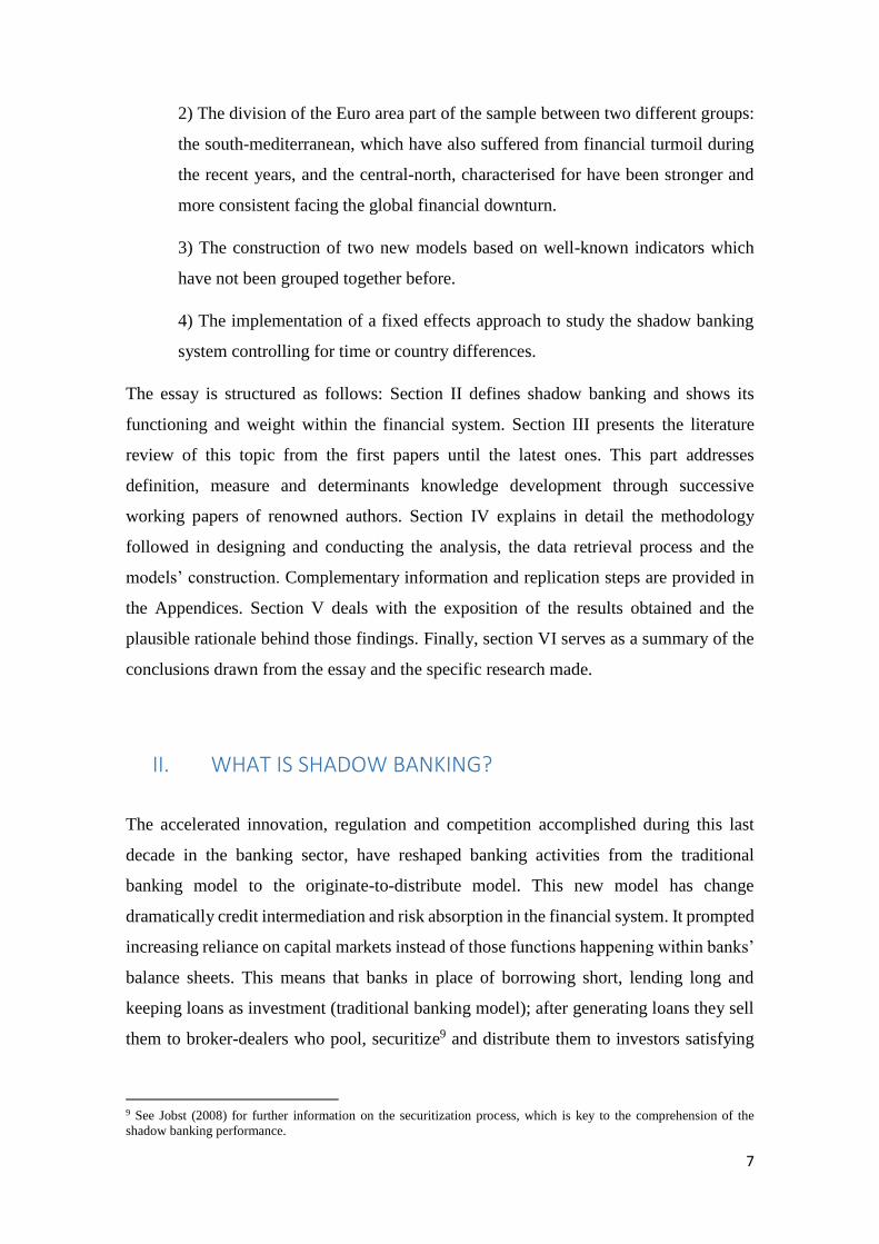
system).10 Exhibit 1 shows information about the tendency of the traditional and shadow

banking financial assets during the period 2010-2014.

Exhibit 1. Assets of financial intermediaries.

Notes: Banks = broader category of “deposit-taking institutions”; OFIs = Other Financial Intermediaries;

Shadow Banking = measure of shadow banking based on economic functions. These are not mutually

exclusive categories, as shadow banking is largely contained in OFIs.

Source: Global Shadow Banking Monitoring Report 2015. Financial Stability Board (FSB).

From a general point of view, the shadow banking system (SBS) can be defined as all the

activities related to credit intermediation, liquidity and maturity transformation that

happens outside the regulated banking system.11 Despite the diverse names authors give

to the shadow banking system, it is clear that they talk about the same concept, although

the existence of slight nuances explained in Section II of this essay.

The size of the SBS depends on the approach taken in its definition and measuring

process. It was showed that around 1995, the level of shadow banking liabilities in the

US overtook the traditional bank level. The distance between liabilities types widened

during the following decade reaching a maximum in 2008-2009.12 In the same vein, the

Financial Stability Board (FSB) has conducted a recent worldwide research on SBS

10 See Pozsar (2008) for deeper explanation in evolution between banking models. 11 See Bakk-Simon et al. (2012). This is the most commonly used shadow banking system definition by the European

Central Bank. Liquidity transformation refers to investing in illiquid assets while acquiring funding through liquid

liabilities. Maturity transformation relates to the use of short-term liabilities to fund investment in long-term assets. 12 See Pozsar et al. (2010).

9

demonstrating its growing importance compared to banks (see Exhibit 1). In this study

made for a 26 jurisdiction sample, it is shown that SBS has been steadily increasing at a

rate of 6% in average during 2011-2014 period. Furthermore, it is demonstrated how this

financial segment’s growth in 2014 was 10.1%, whereas the pace of traditional banks was

6.4%.

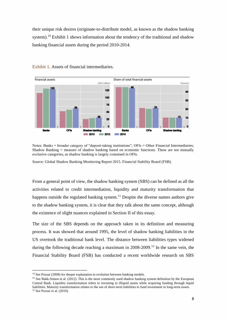
Exhibit 2. Shadow Banking assets share per country

Note: CA = Canada; CN = China; DE = Germany; EMEs ex CN = Argentina, Brazil, Chile, India,

Indonesia, Mexico, Russia, Turkey, Saudi Arabia, South Africa; FR = France; IE = Ireland; JP = Japan; KR

= Korea; NL = Netherlands; UK = United Kingdom; US = United States.

Source: Global Shadow Banking Monitoring Report 2015. Financial Stability Board (FSB).

In Exhibit 2 it is showed the countries’ podium in percentage of shadow banking assets

as a fraction of the total: US (40%), UK (11%), China (8%), Ireland (8%), Germany (7%),

Japan (7%) and France (4%). It is remarkable the impressive increase in the case of China.

This country went from a 2% of the share in 2010 to an 8% in 2014.13 Actually, it is

relevant the fact that, from this FSB sample, more than a half of shadow banking assets

are in hands of US and UK nowadays, revealing the financial power of both countries.

Although the traditional banking system (TBS) and the SBS are thought as mutually

exclusive, they have a high degree of interconnectedness. In Exhibit 3, the reader can

discern what the International Monetary Fund (IMF) presented as a simple explanatory

scheme of the diverse players, the functioning and the flow of funds among SBS players

and also between those and the TBS.

13 See FSB (2015) for methodological process behind those results.

10

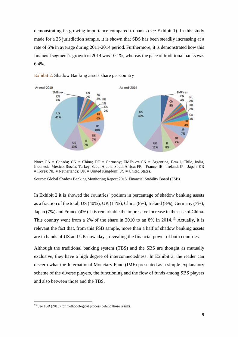
Exhibit 3. Traditional versus Shadow Banking credit intermediation.

Note: lenders category includes institutional investors (ICPFs), central banks and sovereign wealth funds.

Source: International Monetary Fund (2014).

Blue boxes represent the typical players in a traditional banking-based economy where

financial intermediation is made by banks. They raise funds from lenders’ deposits and

give loans to borrowers, making business from interest rates differentials between both

flows. All the grey boxes depict the SBS. Dark grey box called “Finance companies and

other nonbank lenders” represents shadow banking in less developed economies, whereas

inner boxes represents, in broad terms, a developed country non-regulated banking

system. Whereas the main trade in the TBS is capturing deposits (providing loans) in

exchange of interest rate payments (collection), in the SBS system the principal trade is

between securities and money or loans. Thus the process of securitization earns

tremendous relevance in this credit intermediation model.14

14 See footnote 1.

11

III. LITERATURE REVIEW.

III.1 First research on SBS.

The definition of the Shadow Banking System is not straightforward and it depends on

the point of view adopted by the researcher. The term of shadow banking was first coined

by McCulley (2007), as he referred to all the combination of unregulated and heavily

levered up non-bank structures and vehicles. Those unregulated shadow banks fund

themselves with un-insured commercial paper which is not backstopped in case of

liquidity problems. Opposite to the regulated banking system, which has the tools to

overcome liquidity stress such as FRB discount window, the SBS is much more prone to

suffer from runs. First working papers and articles dealing with a deep assessment of the

SBS were made by Pozsar (2008) and Adrian and Shin (2009). A comprehensive

overview of the SBS can be found in Pozsar, Adrian, Ashcraft, and Boesky (2010). In

that paper, the authors foster further discussion on SBS topic while presenting the

features, economic role and relation of it with the traditional banking system. As

McCulley claimed, they also highlight the attractiveness generated by SBS as an

“inexpensive” credit funding source during early 2000s’ real estate boom. Investors’

blindness made them unable to realise the inherent dangerous lack of guarantee schemes

against a possible capital and liquidity shortfall.

III.2 SBS definition.

In one of the first academic papers dealing with SBS, Pozsar (2008), the author defines

SBS as a network of highly levered off-balance sheet credit intermediation vehicles which

is at the heart of the financial crisis. The author differentiates between the traditional

model of banking and the originate-to-distribute model. This distinction is also made by

other authors, as Martinez-Miera and Repullo (2015). In a later paper, Pozsar (2013), the

author improved the definition. He refers to shadow banking as the credit intermediation

chain composed by specialized financial intermediaries, called shadow banks, which are

in charge of traditional banking activities (credit, maturity and liquidity transformation).

These intermediaries perform banking activities without the safety net of having direct

and explicit access to public sources of liquidity or credit backstops.

12

Other authors, as Shin and Shin (2010), focus their attention on the counterpart of the

liability itself. In order to consider a liability as core (estimate of TBS) or non-core

(estimate of SBS) it is necessary to know whom the liability is due to. It will be a core

liability if its counterpart is an ultimate domestic creditor whereas it will be classified as

non-core if its counterpart is an intermediary or a foreign creditor.

Another approach to the SBS is made by Harutyunyan, Massara, Ugazio, Amidzic and

Walton (2015). In this paper the authors claim that the institutional perspective taken by

Pozsar in his first essays, defining shadow banks as institutions outside the banking

system’s regulatory framework, is not accurate enough. They defend the fact that shadow

banking-like liabilities can be potentially issued by all financial institutions involved in

credit intermediation. Authors also give relevance to the counterpart of that kind of

liabilities as in Shin and Shin (2010). However, their essay’s main contribution to the

SBS scope is the focus on the financial instrument’s nature. They distinguish between

core and non-core liabilities. The former are the traditional banking sources of regular

deposits from ultimate domestic creditors and the latter are the SBS-like liabilities.

Furthermore, noncore liabilities can be considered as narrow or broad depending on

whether the measure encompasses intra-SBS positions (asset of one financial corporation

represents the liability of another) or not.

Finally, from an institutional point of view, Bakk-Simon et al. (2012) and the IMF (2014)

define SBS in broader terms. Both use the same definition: SBS are all the activities

related to credit intermediation, liquidity and maturity transformation that happens

outside the regulated banking system, and therefore lacking a formal safety net. However,

it is noticeable the position taken by the IMF of trying to run away from the completely

negative connotation of the SBS. This bad image is mainly due to the interconnectedness

between SBS and the financial crisis. To overcome this idea, the IMF states that SBS can

complement the traditional banking system by expanding access to credit, or by

supporting market liquidity, maturity transformation and risk sharing. As an example,

Gosh, Gonzalez del Mazo and Otker (2012) explained that in developing economies, the

SBS provides a vital service of giving access to credit and investments to under-banked

communities, subprime customers and low-rated firms.

13

III.3 SBS measure.

The most extended measures used in the literature about the SBS so far, have been

computed only from an institutional perspective, due to data availability constraints.

However, the trend is changing from institutional to activity-based approach once enough

valuable data is gradually being obtained (as it is explained in sub-section III.2). There

are two main measures in the literature that deserve to be brought to the review.

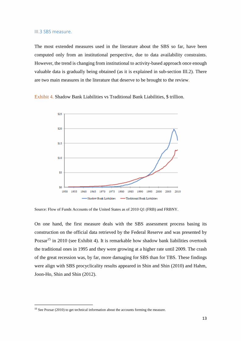
Exhibit 4. Shadow Bank Liabilities vs Traditional Bank Liabilities, $ trillion.

Source: Flow of Funds Accounts of the United States as of 2010 Q1 (FRB) and FRBNY.

On one hand, the first measure deals with the SBS assessment process basing its

construction on the official data retrieved by the Federal Reserve and was presented by

Pozsar15 in 2010 (see Exhibit 4). It is remarkable how shadow bank liabilities overtook

the traditional ones in 1995 and they were growing at a higher rate until 2009. The crash

of the great recession was, by far, more damaging for SBS than for TBS. These findings

were align with SBS procyclicality results appeared in Shin and Shin (2010) and Hahm,

Joon-Ho, Shin and Shin (2012).

15 See Pozsar (2010) to get technical information about the accounts forming the measure.

14

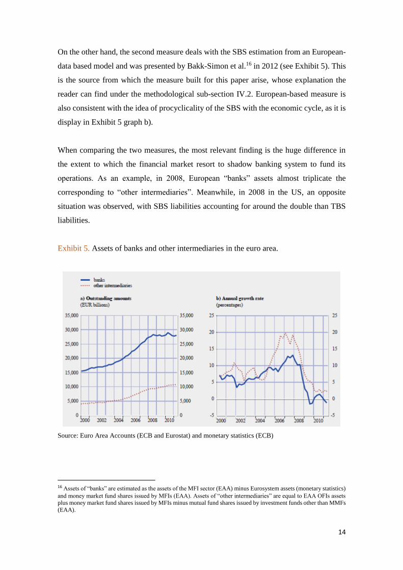
On the other hand, the second measure deals with the SBS estimation from an European-

data based model and was presented by Bakk-Simon et al.16 in 2012 (see Exhibit 5). This

is the source from which the measure built for this paper arise, whose explanation the

reader can find under the methodological sub-section IV.2. European-based measure is

also consistent with the idea of procyclicality of the SBS with the economic cycle, as it is

display in Exhibit 5 graph b).

When comparing the two measures, the most relevant finding is the huge difference in

the extent to which the financial market resort to shadow banking system to fund its

operations. As an example, in 2008, European “banks” assets almost triplicate the

corresponding to “other intermediaries”. Meanwhile, in 2008 in the US, an opposite

situation was observed, with SBS liabilities accounting for around the double than TBS

liabilities.

Exhibit 5. Assets of banks and other intermediaries in the euro area.

Source: Euro Area Accounts (ECB and Eurostat) and monetary statistics (ECB)

16 Assets of “banks” are estimated as the assets of the MFI sector (EAA) minus Eurosystem assets (monetary statistics)

and money market fund shares issued by MFIs (EAA). Assets of “other intermediaries” are equal to EAA OFIs assets

plus money market fund shares issued by MFIs minus mutual fund shares issued by investment funds other than MMFs

(EAA).

15

III.4 SBS determinants.

The study of possible determinants or contributors to the growth of the shadow banking

system is widespread along the literature. The collection of different sources dealing with

variables related to the SBS will serve as a benchmark for this essay. Moreover, it will

support the main essay’s idea of developing quantitative models to study the non-

regulated segment of the financial system.

Researchers have realised the fact that during periods of fast economic development,

traditional banking, as the main source of credit, is not enough to cover the demand of the

market. This scarcity of credit is mainly due to the rigidity of the traditional banking

system (monitoring and legal costs and constraints) which is vanquish by banks and non-

financial credit institutions shifting to “non-traditional” sources. Following this idea,

Hahm, Joon-Ho, Shin and Shin (2012) developed an innovative model of credit supply.

The model supported the hypothesis of procyclicality of non-regulated sector with the

expansion of the balance sheet during a credit boom. Moreover, other authors as Shin and

Shin (2010) have also shown the positive correlation between the non-traditional

liabilities and the business cycle. This business cycle can be measured in terms of Gross

Domestic Product (GDP).

The authors in IMF (2014) established that the search for yield effect17, tighter bank

regulation and grow of the rest of the financial system can be variables that contribute to

the SBS development. Moreover, they conducted a panel regression to quantify for the

effects of some macro-financial variables (e.g. real GDP growth, banking sector size,

institutional investors’ size and term-spread) and some regulatory variables (e.g. overall

capital stringency and global liquidity indicators). The search for yield effect also appears

in other research papers as Martinez-Miera and Repullo (2015). The latter refers to the

search for yield effect in the banking sector, due to gap reduction between interest rates

paid on deposits and interest rates earned on loans; whereas the former focus its attention

on the term-spread squeeze.

17 See Rajan (2005). “Search for yield effect” is defined as an increase in investment risk-taking as a manner to obtain

higher expected return during periods with low interest rates.

16

Duca (2014) studied the drivers of the SBS in the short and the long run. On one hand, he

demonstrated that, in the long-run, SBS is negatively correlated to information costs and

positively correlated to bank reserve requirements and the relative burden of capital

requirements on commercial versus shadow bank credit. On the other hand, he showed

that the shadow banking system share in the short run fell when liquidity premia were

high, and when term premia reflected expectations of economic scenario improvements;

however, it rose when deposit rate ceilings were more stringent and regulatory changes

benefit nonbank compared to bank finance. This SBS procyclicality and vulnerability to

liquidity shocks are consistent with Adrian and Shin (2009a, 2009b, 2010), Brunnermeier

and Sannikov (2013), Geankoplos (2010), and Gorton and Metrick (2012).

III.5 Latest research on SBS.

During last years, the focus has been mainly pointed towards overcoming the shadow

banking institutional-based measure granularity problem. Moreover, it is clearly signalled

the intention to change the approach from institutional to activity-based definition and

measure, once enough data will be retrieved. Apart from that, monitoring process,

financial stability and the Chinese SBS escalation are also heavily attracting researchers´

attention.

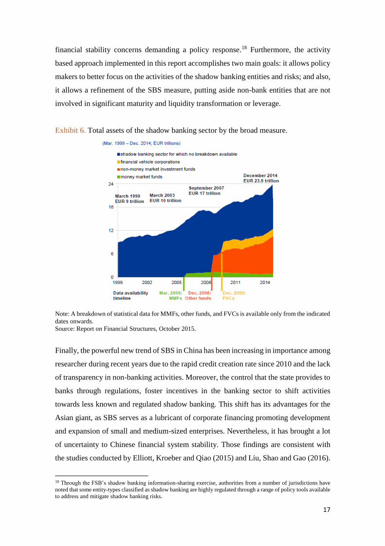
The ECB (2015) showed how the decomposition of the SBS broad measure into different

institutional sub-aggregates has been evolving lately. Light has been shed on those

categories from 2008 until today, once relevant data has started to be computed by

financial authorities (see Exhibit 6). Despite this advances in the SBS assessment, there

is still a 50% of shadow banking assets for which a breakdown is not available. However,

it is known that two thirds of this “residual” part of Euro area SBS assets are held in

Netherlands and Luxembourg.

In the report from FSB (2015), it has been designed a SBS measure based in five different

economic functions, each of which involves non-bank credit intermediation that

potentially pose some financial risks (activity-based approach). Those risks may raise

17

financial stability concerns demanding a policy response.18 Furthermore, the activity

based approach implemented in this report accomplishes two main goals: it allows policy

makers to better focus on the activities of the shadow banking entities and risks; and also,

it allows a refinement of the SBS measure, putting aside non-bank entities that are not

involved in significant maturity and liquidity transformation or leverage.

Exhibit 6. Total assets of the shadow banking sector by the broad measure.

Note: A breakdown of statistical data for MMFs, other funds, and FVCs is available only from the indicated

dates onwards.

Source: Report on Financial Structures, October 2015.

Finally, the powerful new trend of SBS in China has been increasing in importance among

researcher during recent years due to the rapid credit creation rate since 2010 and the lack

of transparency in non-banking activities. Moreover, the control that the state provides to

banks through regulations, foster incentives in the banking sector to shift activities

towards less known and regulated shadow banking. This shift has its advantages for the

Asian giant, as SBS serves as a lubricant of corporate financing promoting development

and expansion of small and medium-sized enterprises. Nevertheless, it has brought a lot

of uncertainty to Chinese financial system stability. Those findings are consistent with

the studies conducted by Elliott, Kroeber and Qiao (2015) and Liu, Shao and Gao (2016).

18 Through the FSB’s shadow banking information-sharing exercise, authorities from a number of jurisdictions have

noted that some entity-types classified as shadow banking are highly regulated through a range of policy tools available

to address and mitigate shadow banking risks.

18

IV. DATA AND METHODOLOGY

This section presents the data retrieved and the different regression analysis conducted

during the research. The methodological explanation describes the following: 1) the

study’s temporal and geographical framework, 2) the measure computed and the variables

analysed, 3) model types, implementation and their extensions 4) some limitations to have

in mind for this essay in particular, and also, some of them can be extrapolated to the

literature written about shadow banking so far.

IV.1 Framework.

The framework in which the analysis is embedded is divided in two different sources of

variation: the temporal and the geographical.

The first source of variation defines the time limits of the research. It sets the quarterly-

based computation of the SBS measure and the independent variables from 1999q1 to

2013q1 (for the countries with the highest data availability of the sample: “core sample”).

The period’s length selection has been made considering two main factors 1) data

availability for some countries of the Euro area (EA) before 1999 is very limited; and 2)

the fact that the analysis is based on comparing Euro area with the United States (US),

and also analysing the trends within the Euro area, it does make sense to establish the

starting point from the very beginning of the euro adoption. Furthermore, the quarterly

periodicity chosen is aligned with the most commonly used in SBS’s economic research.

It allows the analysis to compute for more accurate and detailed variation than an annual

approach. The variables retrieved on an annual basis have been transformed to quarterly

using simple linear interpolation, whereas the monthly ones have been converted using

the pertinent quarter average, as explained in Appendix 1.

The second source of variation is established as the country for which information on the

SBS and the other variables has been computed. The countries selected for data retrieval

are the US, UK and the members of Euro area (19 countries): Austria, Belgium, Cyprus,

Germany, Estonia, Spain, Finland, France, Greece, Ireland, Italy, Lithuania,

Luxembourg, Latvia, Malta, Netherlands, Portugal, Slovakia and Slovenia. The US has

been selected due to its role of most powerful economy nowadays and also because the

19

bigger bulk of research about Shadow Banking topic is related to it. On the other hand,

the selection of all the countries of the Euro area (EA) and UK, has been made for enable

the study to address a faithful sample on reflecting European shadow banking system

evolution and current situation. However, and due to data limitations in some variables

of the study, five countries of the sample have been dropped in all the models: Cyprus,

Estonia, Lithuania, Luxembourg and Malta. Apart from these countries, many others from

EA and also the US are not considered under the robustness tests nor in the extended

model for the same reason.

IV.2 Data description.

The majority of variables selected and analysed in this study have been based on previous

research and literature written by highly recognized experts in the shadow banking and

credit intermediation field. As it can be seen in Section III of this paper, the process of

searching for relations between shadow banking system and macro-financials is widely

share among researchers. Along the following paragraphs, all the variables used will be

defined and also the effect that the former seek to capture will be explained. Furthermore,

it is indicated which of the variables are based on previous studies and, on the contrary,

which have risen from my intuition and knowledge.

The dependent variable used in every model of this essay is the shadow banking measure,

which is called sbsratio. The measure has been computed from a European perspective

based on EA data availability, and it has been replicated for the US making the pertinent

adaptations. As it is not straightforward to compute the same measure in two widely

different financial environments and histories, it is suggested to look into this replication

critically. Differences in building the same measure for EA and US is one of the

limitations of this paper. Technical descriptions of the accounts considered in building

sbsratio are explained in Appendix 2.

In the case of the EA, the ratio is defined as Other Financial Institutions (OFIs, measuring

the shadow banking system) divided by Monetary Financial Institutions (MFIs,

measuring the traditional banking system), as computed by the ECB in the Euro Area

Accounts (EAA). As stated in the FSB (2015), shadow banking activities are largely run

by OFIs. A similar approach of the close relation of OFIs and SBS is made in

20

Harutyunyan et al. (2015) and Bakk-Simon et al. (2012). More precisely, the measure

used in this paper is based on the last-mentioned work. In this report the author estimates

the traditional banking system (TBS) as MFIs assets minus Eurosystem assets and Money

Market Funds (MMFs) shares issued by MFIs; whereas the shadow banking system is

estimated as OFIs assets plus MMFs shares issued by MFIs minus mutual fund shares

issued by investment funds other than MMFs.

The explanation of taking a broader approach in this essay distinguishing only between

OFIs (SBS) and MFIs (TBS) is due to several reasons. First of all, the fact of not having

available MMFs data breakdown before 2008. Secondly, the low MMFs level showed in

general terms in EA once the breakdown was available, with the only exception of some

SBS outliers such as Netherlands and Luxembourg. Moreover, it is arguable subtracting

non-MMFs shares from OFIs, since in the ECB report 2015 it is showed that non-MMFs

contributes to the 40% of the shadow banking whereas MMFs only to the 4%. These are

the reasons why final measure built is considered fair enough to assess shadow banking

level within the study, bearing in mind the huge amount of data availability limitations.

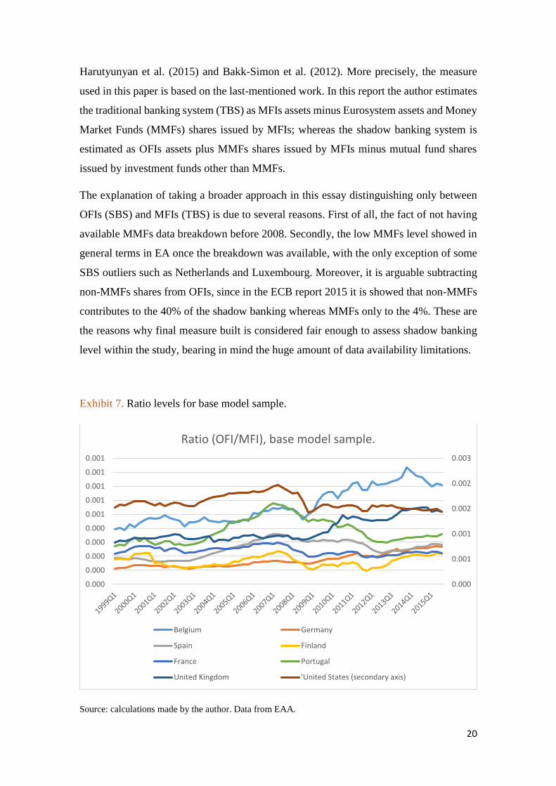
Exhibit 7. Ratio levels for base model sample.

Source: calculations made by the author. Data from EAA.

0.000

0.001

0.001

0.002

0.002

0.003

0.000

0.000

0.000

0.000

0.000

0.001

0.001

0.001

0.001

0.001

Ratio (OFI/MFI), base model sample.

Belgium Germany

Spain Finland

France Portugal

United Kingdom 'United States (secondary axis)

21

In the case of US, the measure is replicated in the following way: first, OFIs assets are

calculated as total financial assets minus central banks, credit institutions, monetary

market mutual funds, property-casualty insurance companies, life insurance companies

and pension funds; second, MFIs assets are computed as central banks plus credit

institutions and money market mutual funds.

As it can be seen in Exhibit 7, the ratio for US is considerably bigger (right y-axis) than

for the rest of the sample, which can be biased due to replication method. Besides, the

existence of two different trends in SBS evolution is distinguishable. Belgium, United

Kingdom and Germany have followed an increasing trend, whereas the rest have suffered

from an up and down peaking process around year 2007.

The independent variables used in this study are the following: 1) GDP at constant prices

(realgdp), 2) institutional investors’ assets (instinv), 3) term-spread (tspread), 4) net

interest margin for banks (margin), 5) liquidity (liquidity), 6) banking concentration index

(hhi), 7) composite indicator of systemic stress (ciss), and 8) inflation (inflation). A

complete explanation on the technical definition, sources and data retrieval process can

be found in Appendix 2.

1) GDP at constant prices, also known as real GDP (realgdp), is the inflation adjusted

value of the goods and services produced by labour and property located inside

corresponding country borders. This variable has been considered as an approach

to measure the procyclicality trait existing between SBS and economic booms and

bursts. The rationale of introducing this variables is based on several studies

already conducted by other researchers.

2) Institutional investors (instinv) are the insurance corporations and pension funds’

assets (ICPFs). This variable has been taken from the IMF (2014). In this report,

the authors related stronger growth of ICPFs with higher growth of SBS and also

a general trend in financial development. Instinv is used to capture

complementarities with SBS and demand-side effects.

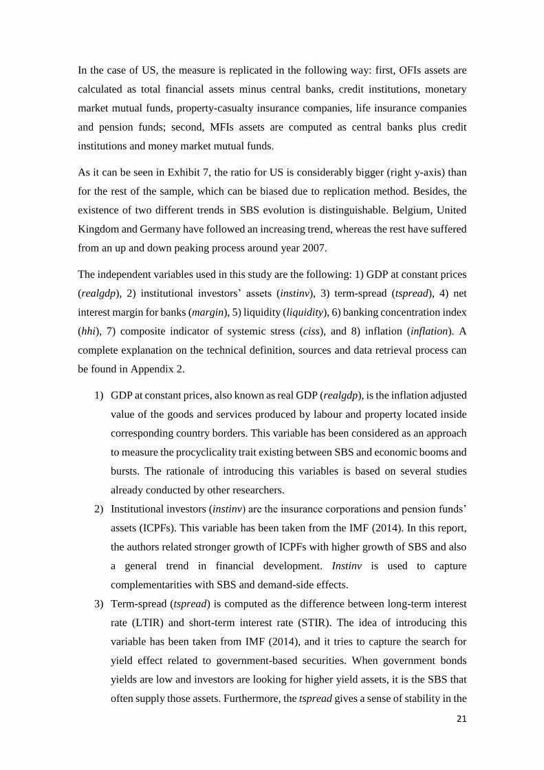
3) Term-spread (tspread) is computed as the difference between long-term interest

rate (LTIR) and short-term interest rate (STIR). The idea of introducing this

variable has been taken from IMF (2014), and it tries to capture the search for

yield effect related to government-based securities. When government bonds

yields are low and investors are looking for higher yield assets, it is the SBS that

often supply those assets. Furthermore, the tspread gives a sense of stability in the

22

economy and the higher the spread, the more investors want to borrow for the long

term. In Exhibit 8, it can be observed the similar trend for all the countries before

2010. After that year, in the countries which suffered from a deeper financial

turmoil the tspread triggered. The case of Portugal clearly stands out.

Exhibit 8. Term-spread evolution.

Source: calculations made by the author. Data from OECD.

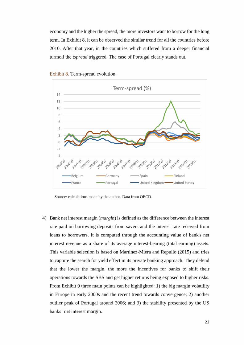
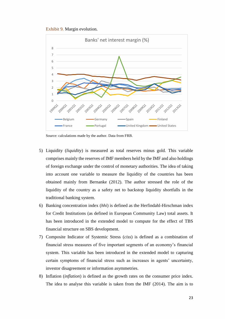
4) Bank net interest margin (margin) is defined as the difference between the interest

rate paid on borrowing deposits from savers and the interest rate received from

loans to borrowers. It is computed through the accounting value of bank's net

interest revenue as a share of its average interest-bearing (total earning) assets.

This variable selection is based on Martinez-Miera and Repullo (2015) and tries

to capture the search for yield effect in its private banking approach. They defend

that the lower the margin, the more the incentives for banks to shift their

operations towards the SBS and get higher returns being exposed to higher risks.

From Exhibit 9 three main points can be highlighted: 1) the big margin volatility

in Europe in early 2000s and the recent trend towards convergence; 2) another

outlier peak of Portugal around 2006; and 3) the stability presented by the US

banks’ net interest margin.

-4

-2

0

2

4

6

8

10

12

14

Term-spread (%)

Belgium Germany Spain Finland

France Portugal United Kingdom United States

23

Exhibit 9. Margin evolution.

Source: calculations made by the author. Data from FRB.

5) Liquidity (liquidity) is measured as total reserves minus gold. This variable

comprises mainly the reserves of IMF members held by the IMF and also holdings

of foreign exchange under the control of monetary authorities. The idea of taking

into account one variable to measure the liquidity of the countries has been

obtained mainly from Bernanke (2012). The author stressed the role of the

liquidity of the country as a safety net to backstop liquidity shortfalls in the

traditional banking system.

6) Banking concentration index (hhi) is defined as the Herfindahl-Hirschman index

for Credit Institutions (as defined in European Community Law) total assets. It

has been introduced in the extended model to compute for the effect of TBS

financial structure on SBS development.

7) Composite Indicator of Systemic Stress (ciss) is defined as a combination of

financial stress measures of five important segments of an economy’s financial

system. This variable has been introduced in the extended model to capturing

certain symptoms of financial stress such as increases in agents’ uncertainty,

investor disagreement or information asymmetries.

8) Inflation (inflation) is defined as the growth rates on the consumer price index.

The idea to analyse this variable is taken from the IMF (2014). The aim is to

0

1

2

3

4

5

6

7

8

Banks' net interest margin (%)

Belgium Germany Spain Finland

France Portugal United Kingdom United States

24

capture the effect of the loss in money purchasing power among investors on their

decisions to shift their investments towards the SBS.

IV.3 Models and extensions.

Once the previous parts of this section have clarified the limits and variables of the

research, it is time to present how the regression models have been built. The models shed

light on the relations existing between independent variables and the SBS through a

multiple regression analysis. The structure of the study is divided in two approaches:

cross-sectional data and panel data, depending on whether Ordinary Least-Squares (OLS)

regression or fixed effects (FE) regression is considered. FE control for some specific

characteristic within the country or the year that may bias the predictor variables outcome.

They remove the effect of those features so it is possible to assess the net effect of the

predictors on the outcome variable.

The cross sectional and panel data studies are composed by two models: the base model

and the extended model. The first one computes the relations between five independent

variables (realgdp, instinv, tspread, margin, and liquidity) and the SBS measure. The

extended one adds to the former another three independent variables (ciss, hhi and

inflation). As data availability varies depending on the considerations taken, a detailed

explanation on the countries composing each of the samples is presented in Appendix 3.

In the cross-sectional part, first an analysis encompassing all the sample is conducted

(whole-sample analysis) for both the base model [Equation 1] and the extended model

[Equation 2]. These regressions serve as a benchmark to compare how the results change

once groups of countries are analysed separately. Second, a “core” base model regression

is run [Equation 1]. The “core” sample is composed by all the countries of the whole-

sample for which data is available from 1999q1 to 2013q1. Moreover, this sample is

divided in four sub-samples depending on both geographical distribution and also on

whether the countries have suffered from a big financial turmoil during the great

recession. The subsamples are the following: the two first are from the EA, being 1)

Belgium, Germany, Finland and France (countries from central and north Europe (C-N)

which have not suffer big financial turmoil) and 2) Spain and Portugal (countries from

south-mediterranean (S-M) Europe which have felt big financial turmoil); 3) United

Kingdom and 4) United States.

25

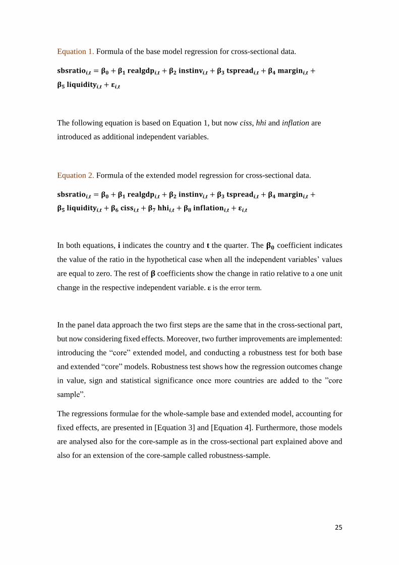
Equation 1. Formula of the base model regression for cross-sectional data.

𝐬𝐛𝐬𝐫𝐚𝐭𝐢𝐨𝒊,𝒕 = 𝛃𝟎 + 𝛃𝟏 𝐫𝐞𝐚𝐥𝐠𝐝𝐩𝒊,𝒕 + 𝛃𝟐 𝐢𝐧𝐬𝐭𝐢𝐧𝐯𝒊,𝒕 + 𝛃𝟑 𝐭𝐬𝐩𝐫𝐞𝐚𝐝𝒊,𝒕 + 𝛃𝟒 𝐦𝐚𝐫𝐠𝐢𝐧𝒊,𝒕 +

𝛃𝟓 𝐥𝐢𝐪𝐮𝐢𝐝𝐢𝐭𝐲𝒊,𝒕 +𝛆𝒊,𝒕

The following equation is based on Equation 1, but now ciss, hhi and inflation are

introduced as additional independent variables.

Equation 2. Formula of the extended model regression for cross-sectional data.

𝐬𝐛𝐬𝐫𝐚𝐭𝐢𝐨𝒊,𝒕 = 𝛃𝟎 + 𝛃𝟏 𝐫𝐞𝐚𝐥𝐠𝐝𝐩𝒊,𝒕 + 𝛃𝟐 𝐢𝐧𝐬𝐭𝐢𝐧𝐯𝒊,𝒕 + 𝛃𝟑 𝐭𝐬𝐩𝐫𝐞𝐚𝐝𝒊,𝒕 + 𝛃𝟒 𝐦𝐚𝐫𝐠𝐢𝐧𝒊,𝒕 +

𝛃𝟓 𝐥𝐢𝐪𝐮𝐢𝐝𝐢𝐭𝐲𝒊,𝒕 + 𝛃𝟔 𝐜𝐢𝐬𝐬𝒊,𝒕 + 𝛃𝟕 𝐡𝐡𝐢𝒊,𝒕 + 𝛃𝟖 𝐢𝐧𝐟𝐥𝐚𝐭𝐢𝐨𝐧𝒊,𝒕 + 𝛆𝒊,𝒕

In both equations, i indicates the country and t the quarter. The 𝛃𝟎 coefficient indicates

the value of the ratio in the hypothetical case when all the independent variables’ values

are equal to zero. The rest of 𝛃 coefficients show the change in ratio relative to a one unit

change in the respective independent variable. ε is the error term.

In the panel data approach the two first steps are the same that in the cross-sectional part,

but now considering fixed effects. Moreover, two further improvements are implemented:

introducing the “core” extended model, and conducting a robustness test for both base

and extended “core” models. Robustness test shows how the regression outcomes change

in value, sign and statistical significance once more countries are added to the ”core

sample”.

The regressions formulae for the whole-sample base and extended model, accounting for

fixed effects, are presented in [Equation 3] and [Equation 4]. Furthermore, those models

are analysed also for the core-sample as in the cross-sectional part explained above and

also for an extension of the core-sample called robustness-sample.

26

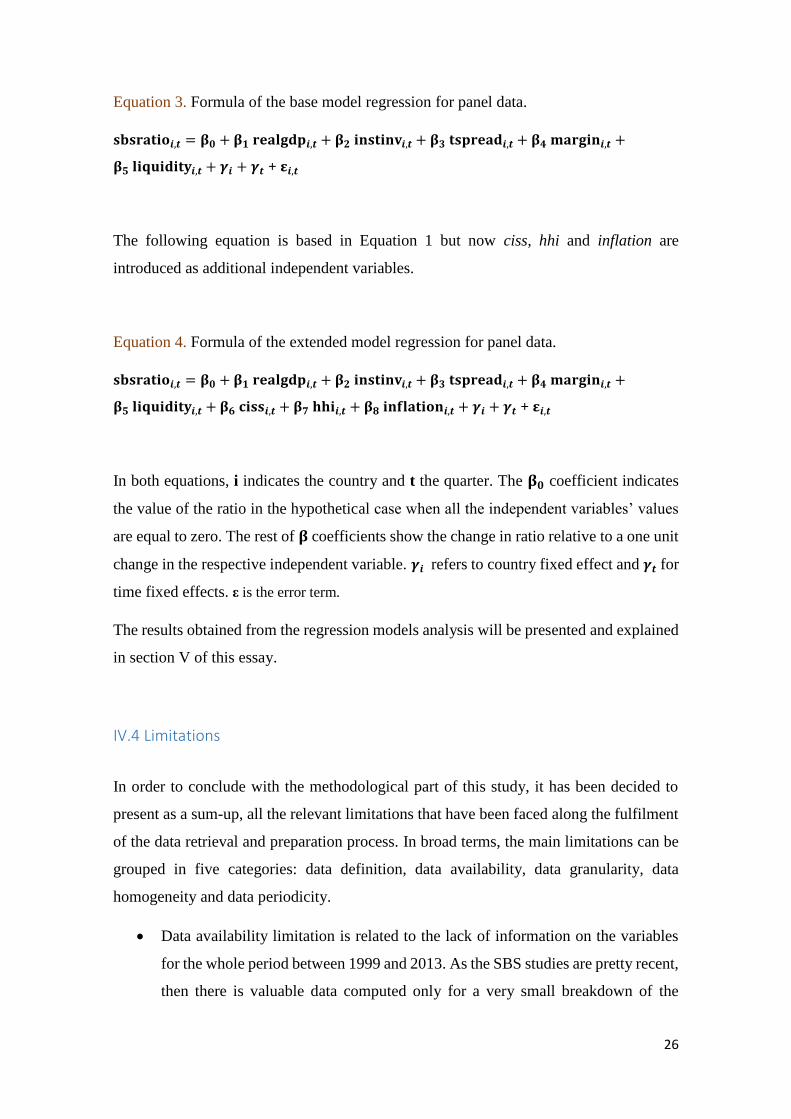
Equation 3. Formula of the base model regression for panel data.

𝐬𝐛𝐬𝐫𝐚𝐭𝐢𝐨𝒊,𝒕 = 𝛃𝟎 + 𝛃𝟏 𝐫𝐞𝐚𝐥𝐠𝐝𝐩𝒊,𝒕 + 𝛃𝟐 𝐢𝐧𝐬𝐭𝐢𝐧𝐯𝒊,𝒕 + 𝛃𝟑 𝐭𝐬𝐩𝐫𝐞𝐚𝐝𝒊,𝒕 + 𝛃𝟒 𝐦𝐚𝐫𝐠𝐢𝐧𝒊,𝒕 +

𝛃𝟓 𝐥𝐢𝐪𝐮𝐢𝐝𝐢𝐭𝐲𝒊,𝒕 + 𝜸𝒊 + 𝜸𝒕 + 𝛆𝒊,𝒕

The following equation is based in Equation 1 but now ciss, hhi and inflation are

introduced as additional independent variables.

Equation 4. Formula of the extended model regression for panel data.

𝐬𝐛𝐬𝐫𝐚𝐭𝐢𝐨𝒊,𝒕 = 𝛃𝟎 + 𝛃𝟏 𝐫𝐞𝐚𝐥𝐠𝐝𝐩𝒊,𝒕 + 𝛃𝟐 𝐢𝐧𝐬𝐭𝐢𝐧𝐯𝒊,𝒕 + 𝛃𝟑 𝐭𝐬𝐩𝐫𝐞𝐚𝐝𝒊,𝒕 + 𝛃𝟒 𝐦𝐚𝐫𝐠𝐢𝐧𝒊,𝒕 +

𝛃𝟓 𝐥𝐢𝐪𝐮𝐢𝐝𝐢𝐭𝐲𝒊,𝒕 + 𝛃𝟔 𝐜𝐢𝐬𝐬𝒊,𝒕 + 𝛃𝟕 𝐡𝐡𝐢𝒊,𝒕 + 𝛃𝟖 𝐢𝐧𝐟𝐥𝐚𝐭𝐢𝐨𝐧𝒊,𝒕 + 𝜸𝒊 + 𝜸𝒕 + 𝛆𝒊,𝒕

In both equations, i indicates the country and t the quarter. The 𝛃𝟎 coefficient indicates

the value of the ratio in the hypothetical case when all the independent variables’ values

are equal to zero. The rest of 𝛃 coefficients show the change in ratio relative to a one unit

change in the respective independent variable. 𝜸𝒊 refers to country fixed effect and 𝜸𝒕 for

time fixed effects. ε is the error term.

The results obtained from the regression models analysis will be presented and explained

in section V of this essay.

IV.4 Limitations

In order to conclude with the methodological part of this study, it has been decided to

present as a sum-up, all the relevant limitations that have been faced along the fulfilment

of the data retrieval and preparation process. In broad terms, the main limitations can be

grouped in five categories: data definition, data availability, data granularity, data

homogeneity and data periodicity.

Data availability limitation is related to the lack of information on the variables

for the whole period between 1999 and 2013. As the SBS studies are pretty recent,

then there is valuable data computed only for a very small breakdown of the

27

developed countries. This fact reduce the possibility to infer reliable

generalizations from the results obtained in regressions.

Data definition issue presents the problem of measuring SBS with data which has

not been designed with that aim. It goes together with the previous limitation.

Data granularity limitation deals with the fact that data is grouped in different

categories by the source, but those are not enough broken down. This fact favours

the reduction on the accuracy of the phenomenon measure because very different

entities in charge of taking diverse credit intermediation activities can be grouped

under the SBS when actually do not contribute to it, or vice versa.

Data homogeneity handicap verse about differences to extrapolate the SBS

measure from the European perspective to the US perspective. Besides, the

impossibility to compute for the three new variables under the extended model

approach has appeared. The heterogeneity in the Euro Area and the so-different

economic evolution path makes it difficult to establish the same accounts

classification for both.

Data periodicity is not actually a big deal. The variables computed monthly,

quarterly and annually can be adapted and transformed to other periodicity, as it

has been done in this research. However, it is true that some precision is lost in

the process. Loss of accuracy depends on the degree of intra-period volatility of

the variable adjusted.

The recent literature developed by governing authorities and international financial

institutions is mainly focused on overcome the three first limitations. In broad terms, the

fourth is more difficult to accomplish due to the widely different historical path follow

by the most relevant countries or group of countries in terms of SBS (US, China, Japan

and EA). The last one depends on the main use for which the data is designed. There are

some variables that are worthless to compute more often because the information added

does not deserve the costs entailed.

28

V. RESULTS

Along this section of the essay the results obtained after conducting the regression

analysis are presented to the reader. The structure explained in the methodology section

of this essay will be followed. It should be reminded that causality cannot be inferred

directly from this results. The main objective of this essay is to discover relevant relations

between each variable and the shadow banking system. The number of observations for

each regression and goodness of fit are showed in Appendix 4.

V.1 Cross-sectional data approach.

Along the following paragraphs, the results analysed are those obtained through OLS

regression method. An OLS multiple regression model consist in using OLS for

predicting the value of a dependent variable (regressand) from the values of two or more

independent variables (regressors). The coefficients corresponding to each regressor

measures its partial effect on the regressand, holding the other variables fixed.

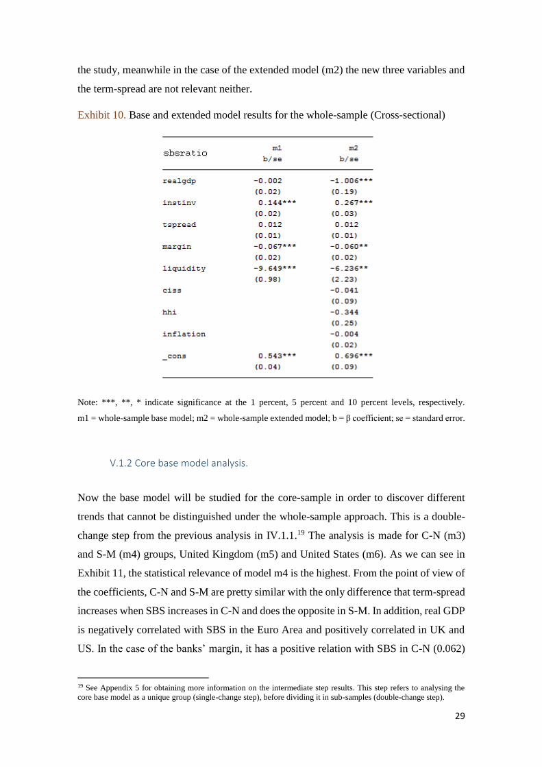
V.1.1 Whole-sample base and extended model analysis.

Before narrowing down the sample to address the two central models of the study, a

regression analysis for each of them has been run taking into account whole countries’

sample in order to have a general view of the raw analysis results. The tables are plotted

in Exhibit 10. Results obtained from this regression are not very significant due to the big

heterogeneity of the sample. However, they are useful as benchmarks to compare the

improvement of the analysis along the process of segmentation of the sample and fixed

effect introduction.

For both models, when institutional investors increase, the SBS ratio increase too

(positive correlation); whereas when the margin widens and the liquidity measure grows,

the SBS ratio decrease (negative correlation). Another reflection on the results of this

approach is the fact that the outcome from the regression signals that in the case of the

base model (m1), the real GDP level and term-spread are not statistically significant for

29

the study, meanwhile in the case of the extended model (m2) the new three variables and

the term-spread are not relevant neither.

Exhibit 10. Base and extended model results for the whole-sample (Cross-sectional)

Note: ***, **, * indicate significance at the 1 percent, 5 percent and 10 percent levels, respectively.

m1 = whole-sample base model; m2 = whole-sample extended model; b = β coefficient; se = standard error.

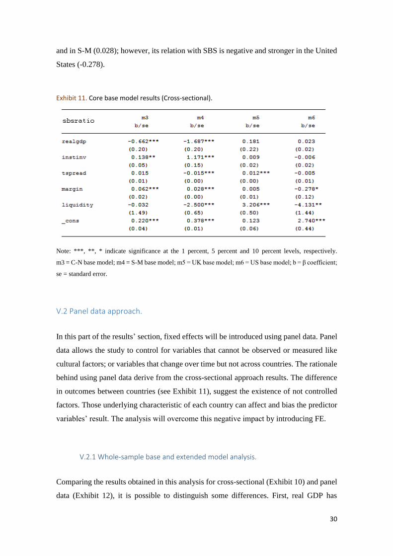
V.1.2 Core base model analysis.

Now the base model will be studied for the core-sample in order to discover different

trends that cannot be distinguished under the whole-sample approach. This is a double-

change step from the previous analysis in IV.1.1.19 The analysis is made for C-N (m3)

and S-M (m4) groups, United Kingdom (m5) and United States (m6). As we can see in

Exhibit 11, the statistical relevance of model m4 is the highest. From the point of view of

the coefficients, C-N and S-M are pretty similar with the only difference that term-spread

increases when SBS increases in C-N and does the opposite in S-M. In addition, real GDP

is negatively correlated with SBS in the Euro Area and positively correlated in UK and

US. In the case of the banks’ margin, it has a positive relation with SBS in C-N (0.062)

19 See Appendix 5 for obtaining more information on the intermediate step results. This step refers to analysing the

core base model as a unique group (single-change step), before dividing it in sub-samples (double-change step).

30

and in S-M (0.028); however, its relation with SBS is negative and stronger in the United

States (-0.278).

Exhibit 11. Core base model results (Cross-sectional).

Note: ***, **, * indicate significance at the 1 percent, 5 percent and 10 percent levels, respectively.

m3 = C-N base model; m4 = S-M base model; m5 = UK base model; m6 = US base model; b = β coefficient;

se = standard error.

V.2 Panel data approach.

In this part of the results’ section, fixed effects will be introduced using panel data. Panel

data allows the study to control for variables that cannot be observed or measured like

cultural factors; or variables that change over time but not across countries. The rationale

behind using panel data derive from the cross-sectional approach results. The difference

in outcomes between countries (see Exhibit 11), suggest the existence of not controlled

factors. Those underlying characteristic of each country can affect and bias the predictor

variables’ result. The analysis will overcome this negative impact by introducing FE.

V.2.1 Whole-sample base and extended model analysis.

Comparing the results obtained in this analysis for cross-sectional (Exhibit 10) and panel

data (Exhibit 12), it is possible to distinguish some differences. First, real GDP has

31

become significant for both models, although the sign is negative for the base model (-

0.023) and positive for the extended (1.413). Second, the banks’ interest margin has lost

its significance for the base model and now is positively related with shadow banking.

Finally, the banking concentration variable (hhi) has improved its significance and shows

negative relation to shadow banking development (-1.081).

Exhibit 12. Base and extended model results for the whole-sample (Panel)

Note: ***, **, * indicate significance at the 1 percent, 5 percent and 10 percent levels, respectively.

m7 = whole-sample base model; m8 = whole-sample extended model; b = β coefficient; se = standard error.

V.2.2 Core base model analysis

Once again, a double-change step is taken from the previous analysis in IV.2.1.20 The

approach to narrowing the base model analysis is divided in two steps: first, analysing the

results from the “core base model” for both European countries’ groups, UK and US.

Secondly, test the robustness of the model in the cases of the European groups by adding

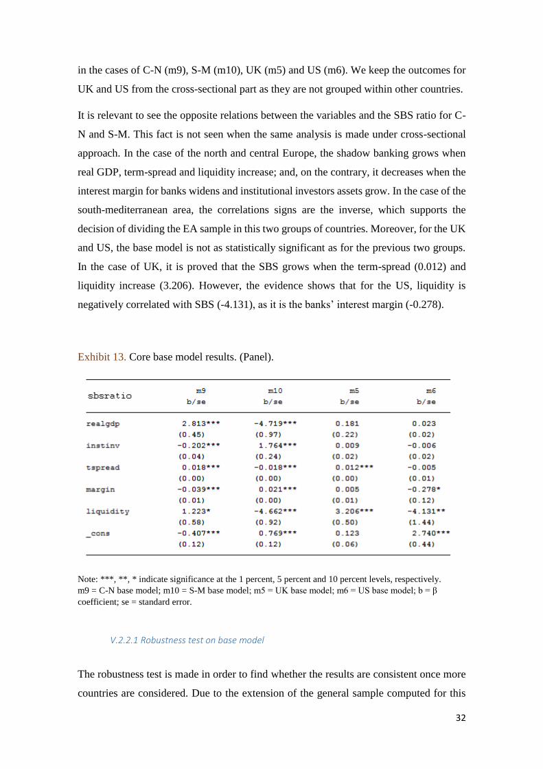
new countries to the sample. Exhibit 13 presents the results of “core base model” analysis

20 See Appendix 6 for obtaining more information on the intermediate step results. This step refers to analysing the

core base model as a unique group (single-change step), before dividing it in sub-samples (double-change step).

32

in the cases of C-N (m9), S-M (m10), UK (m5) and US (m6). We keep the outcomes for

UK and US from the cross-sectional part as they are not grouped within other countries.

It is relevant to see the opposite relations between the variables and the SBS ratio for C-

N and S-M. This fact is not seen when the same analysis is made under cross-sectional

approach. In the case of the north and central Europe, the shadow banking grows when

real GDP, term-spread and liquidity increase; and, on the contrary, it decreases when the

interest margin for banks widens and institutional investors assets grow. In the case of the

south-mediterranean area, the correlations signs are the inverse, which supports the

decision of dividing the EA sample in this two groups of countries. Moreover, for the UK

and US, the base model is not as statistically significant as for the previous two groups.

In the case of UK, it is proved that the SBS grows when the term-spread (0.012) and

liquidity increase (3.206). However, the evidence shows that for the US, liquidity is

negatively correlated with SBS (-4.131), as it is the banks’ interest margin (-0.278).

Exhibit 13. Core base model results. (Panel).

Note: ***, **, * indicate significance at the 1 percent, 5 percent and 10 percent levels, respectively. m9 = C-N base model; m10 = S-M base model; m5 = UK base model; m6 = US base model; b = β

coefficient; se = standard error.

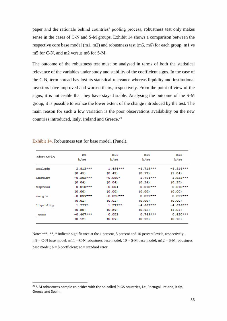
V.2.2.1 Robustness test on base model

The robustness test is made in order to find whether the results are consistent once more

countries are considered. Due to the extension of the general sample computed for this

33

paper and the rationale behind countries’ pooling process, robustness test only makes

sense in the cases of C-N and S-M groups. Exhibit 14 shows a comparison between the

respective core base model (m1, m2) and robustness test (m5, m6) for each group: m1 vs

m5 for C-N, and m2 versus m6 for S-M.

The outcome of the robustness test must be analysed in terms of both the statistical

relevance of the variables under study and stability of the coefficient signs. In the case of

the C-N, term-spread has lost its statistical relevance whereas liquidity and institutional

investors have improved and worsen theirs, respectively. From the point of view of the

signs, it is noticeable that they have stayed stable. Analysing the outcome of the S-M

group, it is possible to realize the lower extent of the change introduced by the test. The

main reason for such a low variation is the poor observations availability on the new

countries introduced, Italy, Ireland and Greece.21

Exhibit 14. Robustness test for base model. (Panel).

Note: ***, **, * indicate significance at the 1 percent, 5 percent and 10 percent levels, respectively.

m9 = C-N base model; m11 = C-N robustness base model; 10 = S-M base model; m12 = S-M robustness

base model; b = β coefficient; se = standard error.

21 S-M robustness-sample coincides with the so-called PIIGS countries, i.e. Portugal, Ireland, Italy, Greece and Spain.

34

V.2.3 Core extended model analysis.

The second model to analyse is the extended model. The approach taken is the same as

in the base model: first, explaining the results for the “core extended model” for both

European countries’ groups (m13 for C-N and m14 for S-M) and UK (m15). Afterwards,

testing the robustness of this model. As it is explained in the methodology section, US is

dropped from this model’s sample due to no data availability in terms of the three new

variables. Exhibit 15 shows the results obtained from this analysis.

Exhibit 15. Core extended model results. (Panel).

Note: ***, **, * indicate significance at the 1 percent, 5 percent and 10 percent levels, respectively. m13 = C-N extended model; m14 = S-M extended model; m15 = UK extended model; b = β coefficient;

se = standard error.

Results suggest that the core extended model outcome maintains the same signs for the

common variables with the core base model in the case of C-N and S-M groups. However,

some variables such as liquidity and realgdp have lost their significance. For UK, the

significance of term spread has been lost but liquidity correlation with SBS ratio keeps

consistently positive and statistically relevant. In terms of the three new variables

introduced, it is remarkable that ciss is only relevant in the case of UK in which when it

decreases, SBS increases. The hhi variable is negatively correlated with SBS ratio for C-

35

N group (-0.769) and positively correlated for S-M group (5.314). Finally, the variable

inflation is positively correlated with shadow banking in the cases of C-N and UK.

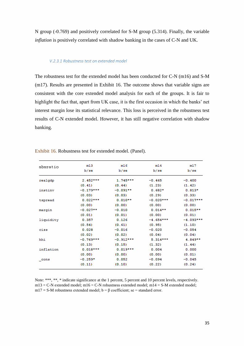
V.2.3.1 Robustness test on extended model

The robustness test for the extended model has been conducted for C-N (m16) and S-M

(m17). Results are presented in Exhibit 16. The outcome shows that variable signs are

consistent with the core extended model analysis for each of the groups. It is fair to

highlight the fact that, apart from UK case, it is the first occasion in which the banks’ net

interest margin lose its statistical relevance. This loss is perceived in the robustness test

results of C-N extended model. However, it has still negative correlation with shadow

banking.

Exhibit 16. Robustness test for extended model. (Panel).

Note: ***, **, * indicate significance at the 1 percent, 5 percent and 10 percent levels, respectively. m13 = C-N extended model; m16 = C-N robustness extended model; m14 = S-M extended model;

m17 = S-M robustness extended model; b = β coefficient; se = standard error.

36

VI. CONCLUSIONS

Shadow banking system (SBS) has played a central role in the recent financial crisis,

though it is a current discussion whether it was a mere amplifier or an originator. This

banking segment provided easy and “inexpensive” access to credit intermediation during

the economic boom of early 2000s. This fact has been argued to contribute to the risk

build-up in the economy. Some countries such as UK and US have a higher, more

developed and deeper rooted shadow banking system than other financially powerful

countries analysed (e.g. Germany and France).

It is certain that shadow banking system is not as negative as its pejorative name implies.

Shadow banking system supplies the financial world with flexible mechanisms to

overcome a rigid and restricted traditional banking system. It even allows under-banked

communities, subprime customers and low-rated firms to get access to credit. However,

its negative impact on financial stability has heavily attracted the attention of governing

authorities. International financial institutions and governments seek to monitor and

regulate shadow banking system to avoid a new worldwide financial catastrophe. In this

vein, the institutional SBS measure used so far, is being changed towards an activity-

based approach, which fits better to shadow banking behaviour. At the same time that

authorities are analysing the real functioning of SBS, a new threat has materialized: the

Chinese shadow banking system escalation.

This paper analyses how the shadow banking level varies when some key determinant

variables change. Those variables are the real GDP, institutional investors’ assets, term-

spread, banks’ net interest margin, liquidity, indicator of systemic stress, banking

concentration measure and inflation. It has been proven that, once controlling for fixed

effects, the SBS and the determinants show opposite relations for central-north (C-N)

than for south-mediterranean (S-M) Euro area. As an example, real GDP has positive

relation with SBS for C-N and negative relation with the S-M sub-sample; and banks’

margin and banking concentration are negatively correlated to SBS in C-N but positively

in S-M. Another conclusion is that the behaviour of the shadow banking system in US is

more similar to C-N Europe than to S-M Europe. Moreover, it has been shown that

robustness tests confirm the consistency of this model when analysing a wider sample of

countries.

37

For all the above-mentioned, this paper suggest that the financial authorities should focus

their attention on these key determinants. Policy making decisions to monitor and control

for shadow banking must be based on the performance observation of these indicators.

Despite the fact that both models analysed are relevant in estimating shadow banking

behaviour, the base model reveals better S-M than C-N fit. The opposite occurs in the

case of the extended model. This information altogether with the opposite sign relations

depending on geography revealed in the previous paragraph, pose European authorities a

big challenge: Which is the best model approach to adopt? Which is the part of the Euro

area that deserves further resources allocation to overcome shadow banking risks? And,

in case that area-specific policies could be implemented to control opposite SBS trends,

how to keep these policies independent between areas in a common monetary and

economic environment?

38

REFERENCES

Adrian, T. & Song Shin, H. 2009, "The shadow banking system: implications for

financial regulation. Federal Reserve Bank of New York Staff Reports, No. 382,

July", Shadow Banking and Systemic Risk: In Search of Regulatory Solutions, vol.

115.

Adrian, T. & Shin, H.S. 2010, "Liquidity and leverage", Journal of financial

intermediation, vol. 19, no. 3, pp. 418-437.

Adrian, T. & Shin, H.S. 2009, "Money, liquidity, and monetary policy", FRB of New

York Staff Report, no. 360.

Bakk-Simon, K., Borgioli, S., Girón, C., Hempell, H.S., Maddaloni, A., Recine, F. &

Rosati, S. 2011, "Shadow banking in the euro area: an overview", ECB occasional

paper, no. 133.

Bernanke, B.S. 2012, "Some reflections on the crisis and the policy response", Remarks

delivered at the Russell Sage Foundation and Century Foundation Conference on

“Rethinking Finance,” New York City, April.

Brunnermeier, M.K. & Sannikov, Y. "The I theory of money".

Duca, J.V., Duca, J.V. & Duca, J.V. 2014, What drives the shadow banking system in

the short and long run?

Elliott, D., Kroeber, A. & Qiao, Y. 2015, "Shadow banking in China: A primer",

Brookings Institution, March.

European Central Bank 2015, "Report on financial structures", Report on financial

structures.

European Central Bank, Glossary. Available:

https://www.ecb.europa.eu/home/glossary/html/index.en.html [2016, April 20th].

European Central Bank, Statistical Data Warehouse. Available:

https://sdw.ecb.europa.eu/browse.do?node=2019184 [2016, April 5th].

Federal Reserve Bank, Federal Reserve Economic Data. Available:

https://research.stlouisfed.org/fred2/series/GDPC1 [2016, April 15th].

Federal Reserve Bank, Financial Accounts of the United States. Available:

https://www.federalreserve.gov/releases/z1/ [2016, April 20th].

Financial Stability Board 2015, "Global Shadow Banking Monitoring Report", FSB

Global Shadow Banking Monitoring Report.

39

Geanakoplos, J. 2010, "The leverage cycle" in NBER Macroeconomics Annual 2009,

Volume 24 University of Chicago Press, pp. 1-65.

Ghosh, S., Gonzalez del Mazo, I. & Ötker-Robe, İ. 2012, "Chasing the shadows: How

significant is shadow banking in emerging markets?"

Gorton, G. & Metrick, A. 2012, "Securitized banking and the run on repo", Journal of

Financial Economics, vol. 104, no. 3, pp. 425-451.

Hahm, J., Shin, H.S. & Shin, K. 2013, "Noncore bank liabilities and financial

vulnerability", Journal of Money, Credit and Banking, vol. 45, no. s1, pp. 3-36.

Harutyunyan, A., Massara, M.A., Ugazio, G., Amidzic, G. & Walton, R. 2015,

Shedding Light on Shadow Banking, International Monetary Fund.

Holló, D., Kremer, M. & Lo Duca, M., A Composite Indicator of Systemic Stress in the

financial system. Available:

https://www.ecb.europa.eu/pub/pdf/scpwps/ecbwp1426.pdf?6d36165d0aa9ae60107

0927f3ab799fc [2016, May 5th].

International Monetary Fund 2014, "Shadow Banking Around the Globe: How Large,

and How Risky?" Chapter 2 in Global Financial Stability Report.

International Monetary Fund, IMF Data. Available:

http://data.imf.org/regular.aspx?key=60998126 [2016, April 24th].

Jobst, A. 2008, "Back to Basics-What Is Securitization?" Finance & Development, vol.

45, no. 3, pp. 48.

Lagarde, C. 2014, "The Challenge Facing the Global Economy: New Momentum to

Overcome a New Mediocre", Speech given at Georgetown University.

Leitner, Y. 2011, "Why do markets freeze?", Federal Reserve Bank of Philadelphia

Business Review, vol. 2, pp. 12-19.

Liu, B., Shao, S. & Gao, Y. 2016, "An Empirical Study about Influence of China’s

Shadow Banking on the Stability of the Financial System", International Journal of

Economics and Finance, vol. 8, no. 4, pp. 104.

Martinez-Miera, D. & Repullo, R. 2015, "Search for Yield".

McCulley, P. 2007, "Teton reflections", PIMCO Global Central Bank Focus, no. 2.

Nasdaq, Nasdaq Investing. Available:

http://www.nasdaq.com/investing/glossary/h/herfindahl-hirschman-index [2016,

April 21st].

OECD, OECD Data. Available: https://data.oecd.org/interest/long-term-interest-

rates.htm [2016, April 15th].

40

Pozsar, Z. 2013, "Institutional cash pools and the Triffin dilemma of the US banking

system", Financial Markets, Institutions & Instruments, vol. 22, no. 5, pp. 283-318.

Pozsar, Z. 2008, "The rise and fall of the shadow banking system", Regional Financial

Review, vol. 44, pp. 1-13.

Pozsar, Z., Adrian, T., Ashcraft, A.B. & Boesky, H. 2010, "Shadow banking", Available

at SSRN 1640545.

Rajan, R.G. 2005, Has financial development made the world riskier?

SancheS, D. 2014, "Shadow Banking and the Crisis of 2007-08", Business Review, no.

Q2, pp. 7-14.

Shin, H.S. & Shin, K. 2011, Procyclicality and monetary aggregates.

The World Bank, World Bank Data. Available:

http://data.worldbank.org/indicator/FI.RES.XGLD.CD [2016, May 1st].

41

ABBREVIATIONS

ABS = Asset-backed security

CISS = Composite Indicator of Systemic Stress

C-N = Central-North

EA = Euro Area

EAA = Euro Area Accounts

ECB = European Central Bank

FE = Fixed Effects

FRB = Federal Reserve Bank

FSB = Financial Stability Board

FVC = Finance Vehicle Corporation

GDP = Gross Domestic Product

HHI = Herfindahl-Hirschman Index

ICPF = Insurance Companies and Pension Funds

IMF = International Monetary Fund

LTIR = Long-term interest rate

MBS = Mortgage-backed security

MFI = Monetary Financial Institution

MMF = Money Market Fund

OFI = Other Financial Institution

OLS = Ordinary Least-Squares

SBS = Shadow banking system

S-M = South-Mediterranean

STIR = Short-term interest rate

TBS = Traditional banking system

42

APPENDICES

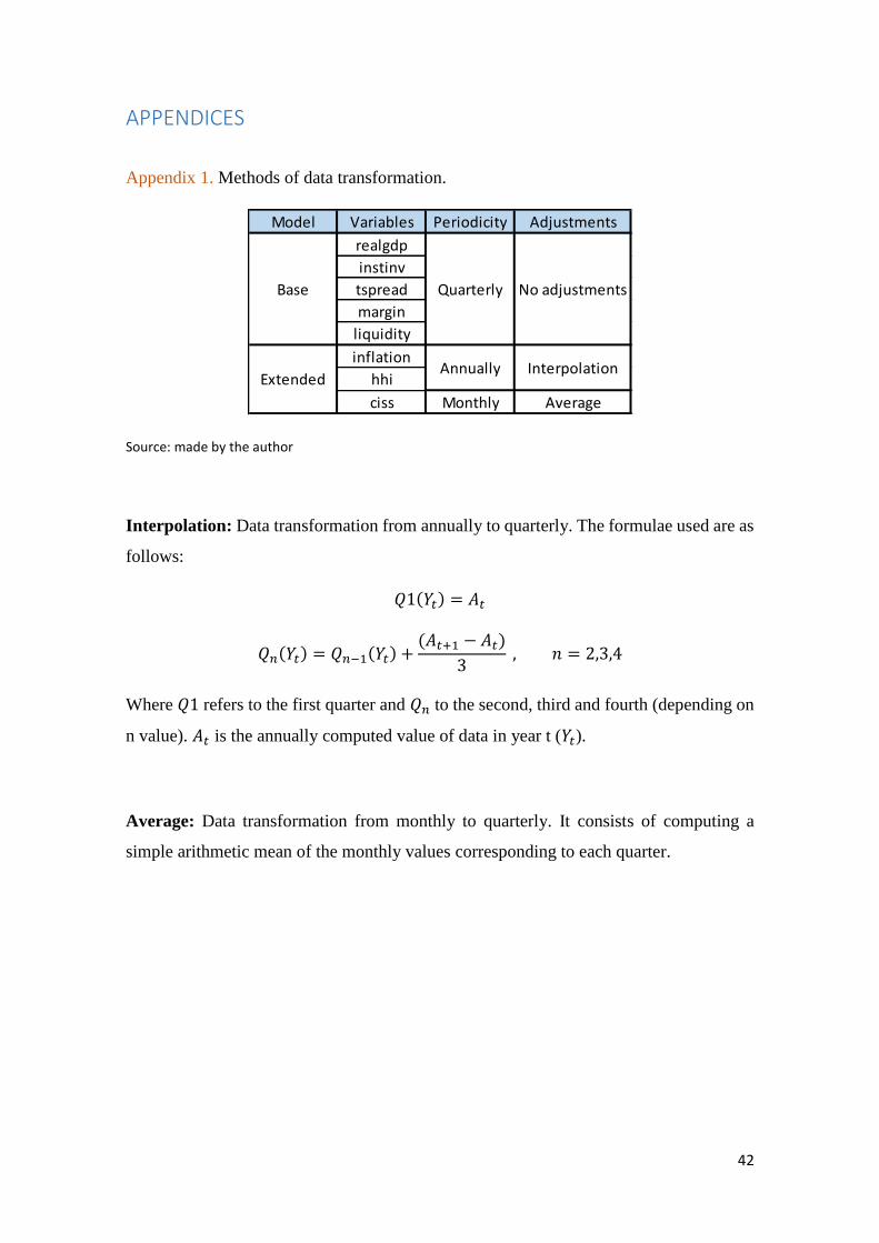
Appendix 1. Methods of data transformation.

Source: made by the author

Interpolation: Data transformation from annually to quarterly. The formulae used are as

follows:

𝑄1(𝑌𝑡) = 𝐴𝑡

𝑄𝑛(𝑌𝑡) = 𝑄𝑛−1(𝑌𝑡) +(𝐴𝑡+1 − 𝐴𝑡)

3 , 𝑛 = 2,3,4

Where 𝑄1 refers to the first quarter and 𝑄𝑛 to the second, third and fourth (depending on

n value). 𝐴𝑡 is the annually computed value of data in year t (𝑌𝑡).

Average: Data transformation from monthly to quarterly. It consists of computing a

simple arithmetic mean of the monthly values corresponding to each quarter.

Model Variables Periodicity Adjustments

realgdp

instinv

tspread

margin

liquidity

inflation

hhi

ciss Monthly Average

Annually InterpolationExtended

Base Quarterly No adjustments

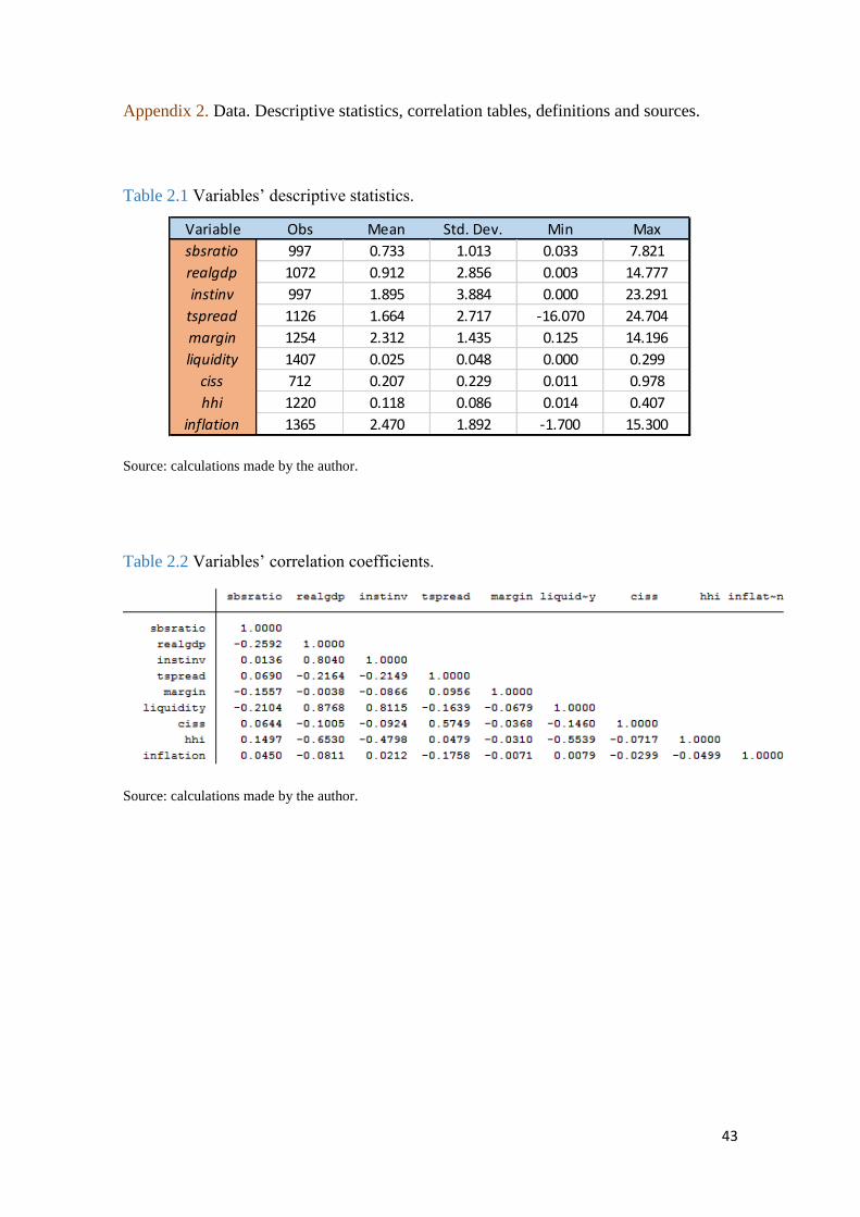
43

Appendix 2. Data. Descriptive statistics, correlation tables, definitions and sources.

Table 2.1 Variables’ descriptive statistics.

Source: calculations made by the author.

Table 2.2 Variables’ correlation coefficients.

Source: calculations made by the author.

Variable Obs Mean Std. Dev. Min Max

sbsratio 997 0.733 1.013 0.033 7.821

realgdp 1072 0.912 2.856 0.003 14.777

instinv 997 1.895 3.884 0.000 23.291

tspread 1126 1.664 2.717 -16.070 24.704

margin 1254 2.312 1.435 0.125 14.196

liquidity 1407 0.025 0.048 0.000 0.299

ciss 712 0.207 0.229 0.011 0.978

hhi 1220 0.118 0.086 0.014 0.407

inflation 1365 2.470 1.892 -1.700 15.300

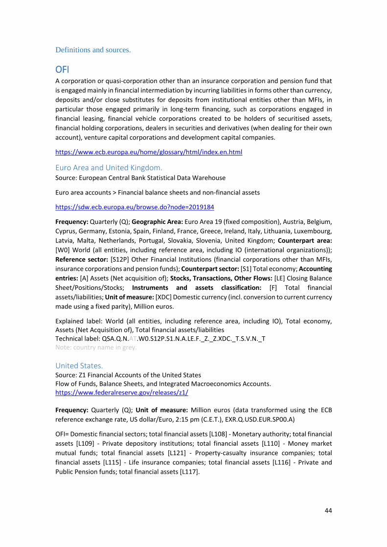
44

Definitions and sources.

OFI A corporation or quasi-corporation other than an insurance corporation and pension fund that

is engaged mainly in financial intermediation by incurring liabilities in forms other than currency,

deposits and/or close substitutes for deposits from institutional entities other than MFIs, in

particular those engaged primarily in long-term financing, such as corporations engaged in

financial leasing, financial vehicle corporations created to be holders of securitised assets,

financial holding corporations, dealers in securities and derivatives (when dealing for their own

account), venture capital corporations and development capital companies.

https://www.ecb.europa.eu/home/glossary/html/index.en.html

Euro Area and United Kingdom. Source: European Central Bank Statistical Data Warehouse

Euro area accounts > Financial balance sheets and non-financial assets

https://sdw.ecb.europa.eu/browse.do?node=2019184

Frequency: Quarterly (Q); Geographic Area: Euro Area 19 (fixed composition), Austria, Belgium,

Cyprus, Germany, Estonia, Spain, Finland, France, Greece, Ireland, Italy, Lithuania, Luxembourg,

Latvia, Malta, Netherlands, Portugal, Slovakia, Slovenia, United Kingdom; Counterpart area:

[W0] World (all entities, including reference area, including IO (international organizations));

Reference sector: [S12P] Other Financial Institutions (financial corporations other than MFIs,

insurance corporations and pension funds); Counterpart sector: [S1] Total economy; Accounting

entries: [A] Assets (Net acquisition of); Stocks, Transactions, Other Flows: [LE] Closing Balance

Sheet/Positions/Stocks; Instruments and assets classification: [F] Total financial

assets/liabilities; Unit of measure: [XDC] Domestic currency (incl. conversion to current currency

made using a fixed parity), Million euros.

Explained label: World (all entities, including reference area, including IO), Total economy, Assets (Net Acquisition of), Total financial assets/liabilities Technical label: QSA.Q.N.AT.W0.S12P.S1.N.A.LE.F._Z._Z.XDC._T.S.V.N._T Note: country name in grey.

United States. Source: Z1 Financial Accounts of the United States Flow of Funds, Balance Sheets, and Integrated Macroeconomics Accounts. https://www.federalreserve.gov/releases/z1/ Frequency: Quarterly (Q); Unit of measure: Million euros (data transformed using the ECB

reference exchange rate, US dollar/Euro, 2:15 pm (C.E.T.), EXR.Q.USD.EUR.SP00.A)

OFI= Domestic financial sectors; total financial assets [L108] - Monetary authority; total financial

assets [L109] - Private depository institutions; total financial assets [L110] - Money market

mutual funds; total financial assets [L121] - Property-casualty insurance companies; total

financial assets [L115] - Life insurance companies; total financial assets [L116] - Private and

Public Pension funds; total financial assets [L117].

45

MFI Financial institutions which together form the money-issuing sector of the euro area. These

include the Eurosystem, resident credit institutions (as defined in EU law) and all other resident

financial institutions whose business is to receive deposits and/or close substitutes for deposits

from entities other than MFIs and, for their own account (at least in economic terms), to grant

credit and/or invest in securities. The latter group consists predominantly of money market

funds.

https://www.ecb.europa.eu/home/glossary/html/index.en.html

Euro Area and United Kingdom. Source: European Central Bank Statistical Data Warehouse

Euro area accounts > Financial balance sheets and non-financial assets

https://sdw.ecb.europa.eu/browse.do?node=2019184

Frequency: Quarterly (Q); Geographic Area: Euro Area 19 (fixed composition), Austria, Belgium,

Cyprus, Germany, Estonia, Spain, Finland, France, Greece, Ireland, Italy, Lithuania, Luxembourg,

Latvia, Malta, Netherlands, Portugal, Slovakia, Slovenia, United Kingdom; Counterpart area:

[W0] World (all entities, including reference area, including IO (international organizations));

Reference sector: [S12K] Monetary Financial Institutions; Counterpart sector: [S1] Total

economy; Accounting entries: [A] Assets (Net acquisition of); Stocks, Transactions, Other Flows:

[LE] Closing Balance Sheet/Positions/Stocks; Instruments and assets classification: [F] Total

financial assets/liabilities; Unit of measure: [XDC] Domestic currency (incl. conversion to current

currency made using a fixed parity), Million euros.

Explained label: World (all entities, including reference area, including IO), Total economy, Assets (Net Acquisition of), Total financial assets/liabilities Technical label: QSA.Q.N.I8.W0.S12K.S1.N.A.LE.F._Z._Z.XDC._T.S.V.N._T Note: country name in grey.

United States. Source: Z1 Financial Accounts of the United States Flow of Funds, Balance Sheets, and Integrated Macroeconomics Accounts. https://www.federalreserve.gov/releases/z1/

Frequency: Quarterly (Q); Unit of measure: Million euros (data transformed using the ECB

reference exchange rate, US dollar/Euro, 2:15 pm (C.E.T.), EXR.Q.USD.EUR.SP00.A)

MFI= Monetary authority; total financial assets [L109] + Private depository institutions; total financial assets [L110] + Money market mutual funds; total financial assets [L121].

46

REAL GROSS DOMESTIC PRODUCT. Real gross domestic product is the inflation adjusted value of the goods and services produced

by labour and property located in a country.

https://research.stlouisfed.org/fred2/series/GDPC1

Euro Area and United Kingdom. Source: Federal Reserve Bank of St. Louis. (retrieved from Eurostat).

Home > FRED® Economic Data > Releases > Gross Domestic Product

https://research.stlouisfed.org/fred2/

Frequency: Quarterly (Q); Geographic Area: Austria, Belgium, Germany, Spain, Finland, France,

Greece, Ireland, Italy, Latvia, Netherlands, Portugal, Slovakia, Slovenia, United Kingdom; Unit of

measure: Thousand Billion of Chained 2010 Euros; Seasonally and calendar adjusted data.

Technical label:

Eurostat unit ID: CLV10_MNAC

Eurostat item ID = B1GQ

Eurostat country ID: XX

For euro area member states, the national currency series are converted into euros using the

irrevocably fixed exchange rate. This preserves the same growth rates than for the previous

national currency series. Both series coincide for years after accession to the euro area but

differ for earlier years due to market exchange rate movements.

United States. Source: Federal Reserve Bank of St. Louis.

Home > FRED® Economic Data > Releases > Gross Domestic Product

https://research.stlouisfed.org/fred2/series/GDPC1

Frequency: Quarterly (Q); Geographic Area: United States; Unit of measure: Thousand billion

of Chained 2009 Euros (data transformed from Thousand Billion of Chained 2009 Dollars using

the ECB reference exchange rate, US dollar/Euro, 2:15 pm (C.E.T.), EXR.Q.USD.EUR.SP00.A);

Seasonally and calendar adjusted data.

Technical label: BEA Account Code: A191RX1

47

INSTITUTIONAL INVESTORS. This variable is considered due to its introduction in the paper IMF October 2014 as “Assets of

insurance companies and pension funds”. According to the ESA 2010, the insurance corporations

subsector consists of all financial corporations and quasi-corporations which are principally

engaged in financial intermediation as a consequence of the pooling of risks mainly in the form

of direct insurance or reinsurance; the pension funds subsector consists of all financial

corporations and quasi-corporations which are principally engaged in financial intermediation

as the consequence of the pooling of social risks and needs of the insured persons (social

insurance). Pension funds as social insurance schemes provide income in retirement, and often

benefits for death and disability.

https://www.ecb.europa.eu/home/glossary/html/index.en.html

Euro Area and United Kingdom. Source: European Central Bank Statistical Data Warehouse

Euro area accounts > Financial balance sheets and non-financial assets

https://sdw.ecb.europa.eu/browse.do?node=2019184

Frequency: Quarterly (Q); Geographic Area: Euro Area 19 (fixed composition), Austria, Belgium,

Cyprus, Germany, Estonia, Spain, Finland, France, Greece, Ireland, Italy, Lithuania, Luxembourg,

Latvia, Malta, Netherlands, Portugal, Slovakia, Slovenia, United Kingdom; Counterpart area:

[W0] World (all entities, including reference area, including IO (international organizations));

Reference sector: [S12Q] Insurance corporations and Pension Funds; Counterpart sector: [S1]

Total economy; Accounting entries: [A] Assets (Net acquisition of); Stocks, Transactions, Other

Flows: [LE] Closing Balance Sheet/Positions/Stocks; Instruments and assets classification: [F]

Total financial assets/liabilities; Unit of measure: [XDC] Domestic currency (incl. conversion to

current currency made using a fixed parity). Thousand Billion Euros.

Explained label: World (all entities, including reference area, including IO), Total economy, Assets (Net Acquisition of), Total financial assets/liabilities Technical label: QSA.Q.N.SK.W0.S12Q.S1.N.A.LE.F._Z._Z.XDC._T.S.V.N._T

Note: country name in grey

United States. Source: Z1 Financial Accounts of the United States Flow of Funds, Balance Sheets, and Integrated Macroeconomics Accounts. https://www.federalreserve.gov/releases/z1/ Frequency: Quarterly (Q); Unit of measure: Thousand Billion Euros (data transformed using the

ECB reference exchange rate, US dollar/Euro, 2:15 pm (C.E.T.), EXR.Q.USD.EUR.SP00.A)

INSTITUTIONAL INVESTORS= Property-casualty insurance companies; total financial assets

[L115] + Life insurance companies; total financial assets [L116] + Private and Public Pension

funds; total financial assets [L117].

48

TERM SPREAD. This variable is computed as the difference between LTIR and STIR.

LONG TERM INTEREST RATE. Long-term interest rates refer to government bonds maturing in ten years. Rates are mainly

determined by the price charged by the lender, the risk from the borrower and the fall in the

capital value. Long-term interest rates are generally averages of daily rates, measured as a

percentage. These interest rates are implied by the prices at which the government bonds are

traded on financial markets, not the interest rates at which the loans were issued. In all cases,

they refer to bonds whose capital repayment is guaranteed by governments. Long-term interest

rates are one of the determinants of business investment. Low long-term interest rates

encourage investment in new equipment and high interest rates discourage it. Investment is, in

turn, a major source of economic growth.

https://data.oecd.org/interest/long-term-interest-rates.htm

Euro Area, United Kingdom and United States. Source: OECD Data

Interest rates.

https://data.oecd.org/interest/long-term-interest-rates.htm

Frequency: Quarterly (Q); Geographic Area: Euro Area 19 (fixed composition), Austria, Belgium,

Germany, Spain, Finland, France, Greece, Ireland, Italy, Latvia, Netherlands, Portugal, Slovakia,

Slovenia, United Kingdom, United States; Unit of measure: Percent per annum.

SHORT TERM INTEREST RATE. Short-term interest rates are the rates at which short-term borrowings are effected between

financial institutions or the rate at which short-term government paper is issued or traded in the

market. Short-term interest rates are generally averages of daily rates, measured as a

percentage. Short-term interest rates are based on three-month money market rates where

available. Typical standardised names are "money market rate" and "treasury bill rate".

https://data.oecd.org/interest/short-term-interest-rates.htm

Euro Area, United Kingdom and United States. Source: OECD Data

Interest rates.

https://data.oecd.org/interest/short-term-interest-rates.htm

Frequency: Quarterly (Q); Geographic Area: Euro Area 19 (fixed composition), Austria, Belgium,

Germany, Spain, Finland, France, Greece, Ireland, Italy, Latvia, Netherlands, Portugal, Slovakia,

Slovenia, United Kingdom, United States; Unit of measure: Percent per annum.

49

NET INTEREST MARGIN. Accounting value of bank's net interest revenue as a share of its average interest-bearing (total

earning) assets.

https://research.stlouisfed.org/fred2/search?st=NET+INTEREST+MARGIN

Euro Area, United Kingdom and United States. Source: Federal Reserve Economic Data.

https://research.stlouisfed.org/fred2/search?st=NET+INTEREST+MARGIN

Frequency: Annual (A) (transformed into Quarterly by linear interpolation); Geographic Area:

Austria, Belgium, Cyprus, Germany, Estonia, Spain, Finland, France, Greece, Ireland, Italy,

Lithuania, Luxembourg, Latvia, Malta, Netherlands, Portugal, Slovakia, Slovenia, United

Kingdom, United States; Unit of measure: percentage.

LIQUIDITY. Liquidity measured as total reserves. Total reserves minus gold comprise special drawing rights,

reserves of IMF members held by the IMF, and holdings of foreign exchange under the control

of monetary authorities. Gold holdings are excluded. Data are in current U.S. dollars.

http://data.worldbank.org/indicator/FI.RES.XGLD.CD

Euro Area, United Kingdom and United States. Source: International Financial Statistics (IFS) Reserves selected indicators

http://data.imf.org/regular.aspx?key=60998126

Frequency: Quarterly (Q); Geographic Area: Euro Area 19(fixed composition), Austria, Belgium,

Cyprus, Germany, Estonia, Spain, Finland, France, Greece, Ireland, Italy, Lithuania, Luxembourg,

Latvia, Malta, Netherlands, Portugal, Slovakia, Slovenia, United Kingdom, United States; Unit of

measure: Thousand Billion Euros (data transformed using the ECB reference exchange rate, US

dollar/Euro, 2:15 pm (C.E.T.), EXR.Q.USD.EUR.SP00.A).

50

COMPOSITE INDICATOR OF SYSTEMIC STRESS (CISS). The CISS (Composite Indicator of Systemic Stress) comprises the five arguably most important

segments of an economy’s financial system: the sector of bank and non-bank financial

intermediaries, money markets, securities (equities and bonds) markets as well as foreign

exchange markets. The current level of stress in each of these five segments is measured on the

basis of three raw stress indicators capturing certain symptoms of financial stress such as

increases in agents’ uncertainty, investor disagreement or information asymmetries. Certain

raw stress indicators shall also capture flight-to-quality and flight-to-liquidity effects,

respectively. The CISS measures such stress symptoms mainly on the basis of securities market

indicators which are quite standard in the literature (such as volatilities, risk spreads and

cumulative valuation losses).

https://www.ecb.europa.eu/pub/pdf/scpwps/ecbwp1426.pdf?6d36165d0aa9ae601070927f3a

b799fc

Euro Area and United Kingdom. Source: European Central Bank Statistical Data Warehouse

Home > Economic Concepts > Monetary and financial statistics > Composite Indicator of

Systemic Stress

https://sdw.ecb.europa.eu/browse.do?node=9551138

Frequency: Monthly (M) (transformed into Quarterly by linear interpolation); Geographic Area:

Austria, Belgium, Germany, Spain, Finland, France, Greece, Ireland, Italy, Netherlands, Portugal,

United Kingdom; Financial market instrument: [EC] Economic indicator; Financial market

provider identifier: [SOV_CI] Sovereign Systemic Stress Composite Indicator; Financial market

data type: [IDX] Index; Unit of measure: pure number.

Technical label: CISS.M.AT.Z0Z.4F.EC.SOV_CI.IDX

Note: country name in grey.

51

HERFINDAHL-HIRSCHMAN INDEX (HHI). A measure of market concentration, it depends on the number of firms and their size relative to

the market. It is calculated by summing up the squares of market shares of each firm.

http://www.nasdaq.com/investing/glossary/h/herfindahl-hirschman-index

Euro Area and United Kingdom. Source: European Central Bank Statistical Data Warehouse

Home > Economic Concepts > Monetary and financial statistics > Structural Financial Indicators

https://sdw.ecb.europa.eu/browse.do?node=9484387

Frequency: Annual (A) (transformed into Quarterly by linear interpolation); Geographic Area:

Austria, Belgium, Cyprus, Germany, Estonia, Spain, Finland, France, Greece, Ireland, Italy,

Lithuania, Luxembourg, Latvia, Malta, Netherlands, Portugal, Slovakia, Slovenia, United

Kingdom; Structural statist indicator: [H10] Herfindahl index for Credit Institutions (CIs) total

assets; Unit of measure: percentage.

Technical label: SSI.A.AT.122C.H10.X.U6.Z0Z.Z

Note: country name in grey.

INFLATION RATE. The measure of the variation of the increase in the general price level.

https://www.ecb.europa.eu/home/glossary/html/index.en.html

Euro Area and United Kingdom. Source: European Central Bank Statistical Data Warehouse

Home > Economic Concepts > Prices, output, demand and labour market > Prices > Consumer

price indices.

https://sdw.ecb.europa.eu/browse.do?node=2120778

Frequency: Annual (A) (transformed into Quarterly by linear interpolation); Geographic Area:

Austria, Belgium, Cyprus, Germany, Estonia, Spain, Finland, France, Greece, Ireland, Italy,

Lithuania, Luxembourg, Latvia, Malta, Netherlands, Portugal, Slovakia, Slovenia, United

Kingdom; Classification-ICP context: [000000] HICP- Overall Index; Series variation-ICP context:

[AVR] Annual average rate of change; Unit of measure: percentage change.

Technical label: ICP.A.AT.N.000000.4.AVR

Note: country name in grey.

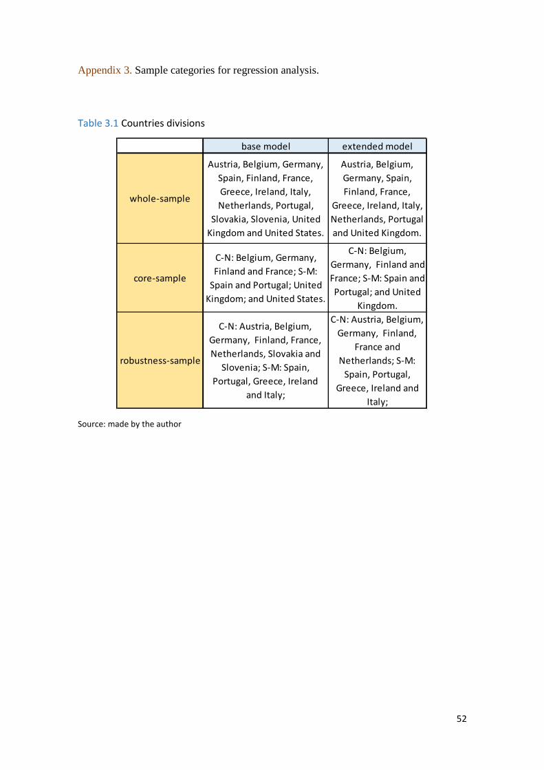
52

Appendix 3. Sample categories for regression analysis.

Table 3.1 Countries divisions

Source: made by the author

base model extended model

whole-sample

Austria, Belgium, Germany,

Spain, Finland, France,

Greece, Ireland, Italy,

Netherlands, Portugal,

Slovakia, Slovenia, United

Kingdom and United States.

Austria, Belgium,

Germany, Spain,

Finland, France,

Greece, Ireland, Italy,

Netherlands, Portugal

and United Kingdom.

core-sample

C-N: Belgium, Germany,

Finland and France; S-M:

Spain and Portugal; United

Kingdom; and United States.

C-N: Belgium,

Germany, Finland and

France; S-M: Spain and

Portugal; and United

Kingdom.

robustness-sample

C-N: Austria, Belgium,

Germany, Finland, France,

Netherlands, Slovakia and

Slovenia; S-M: Spain,

Portugal, Greece, Ireland

and Italy;

C-N: Austria, Belgium,

Germany, Finland,

France and

Netherlands; S-M:

Spain, Portugal,

Greece, Ireland and

Italy;

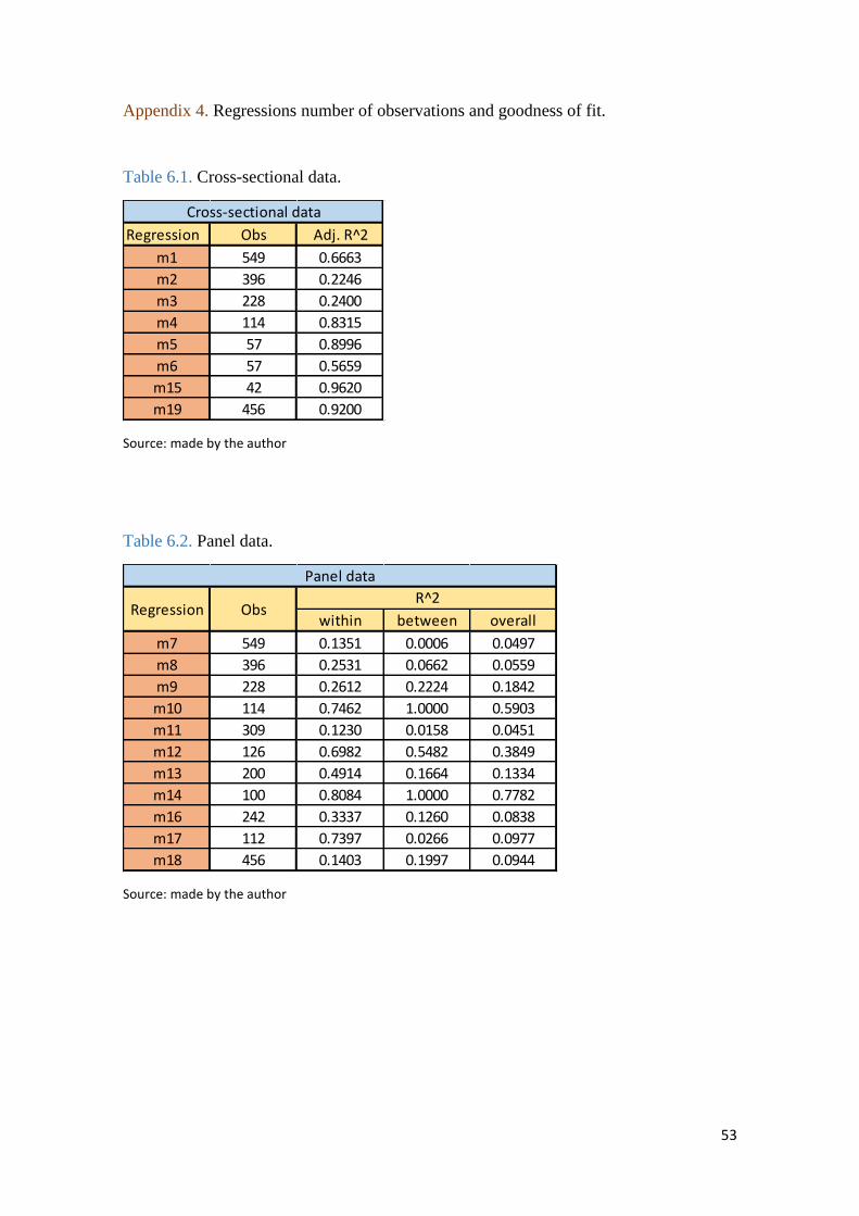
53

Appendix 4. Regressions number of observations and goodness of fit.

Table 6.1. Cross-sectional data.

Source: made by the author

Table 6.2. Panel data.

Source: made by the author

Regression Obs Adj. R^2

m1 549 0.6663

m2 396 0.2246

m3 228 0.2400

m4 114 0.8315

m5 57 0.8996

m6 57 0.5659

m15 42 0.9620

m19 456 0.9200

Cross-sectional data

within between overall

m7 549 0.1351 0.0006 0.0497

m8 396 0.2531 0.0662 0.0559

m9 228 0.2612 0.2224 0.1842

m10 114 0.7462 1.0000 0.5903

m11 309 0.1230 0.0158 0.0451

m12 126 0.6982 0.5482 0.3849

m13 200 0.4914 0.1664 0.1334

m14 100 0.8084 1.0000 0.7782

m16 242 0.3337 0.1260 0.0838

m17 112 0.7397 0.0266 0.0977

m18 456 0.1403 0.1997 0.0944

Panel data

R^2ObsRegression

54

Appendix 5. Base model for whole-sample and one-group core-sample. (Cross-

sectional).

Note: ***, **, * indicate significance at the 1 percent, 5 percent and 10 percent levels, respectively.

m1 = whole-sample base model; m19 = one-group core-sample base model; b = β coefficient; se = standard

error.

As it can be seen in the table, some results change if the base model regression is run for

the whole sample (m1) or for the core-sample as a unique group (m19). The three most

relevant variations are 1) the increase in statistical significance of realgdp, and also its

change of sign; 2) the change in the sign of margin; and 3) decrease in absolute value of

the liquidity coefficient.

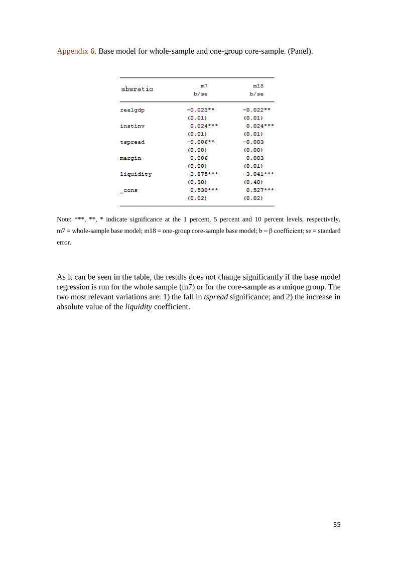
55

Appendix 6. Base model for whole-sample and one-group core-sample. (Panel).

Note: ***, **, * indicate significance at the 1 percent, 5 percent and 10 percent levels, respectively.

m7 = whole-sample base model; m18 = one-group core-sample base model; b = β coefficient; se = standard

error.

As it can be seen in the table, the results does not change significantly if the base model

regression is run for the whole sample (m7) or for the core-sample as a unique group. The

two most relevant variations are: 1) the fall in tspread significance; and 2) the increase in

absolute value of the liquidity coefficient.