1

Paper 883-2017

What Statisticians Should Know about Machine Learning D. Richard Cutler

Utah State University

ABSTRACT In the last few years machine learning/statistical learning methods have gained increasing popularity among data scientists and analysts. Statisticians have sometimes been reluctant to embrace these methodologies, partly due to a lack of familiarity, and partly due to concerns with interpretability and usability. In fact, statisticians have a lot to gain by using this these modern, highly computational tools. For certain kinds of problems machine learning methods can be much more accurate predictors than traditional methods for regression and classification and some of these methods are particularly well suited for the analysis of “big” and “wide” data. Many of these methods have origins in statistics or at the boundary of statistics and computer science and some are already well established in statistical procedures, including LASSO and elastic net for model selection and cross-validation for model evaluation. In this paper I present some examples illustrating the application of machine learning methods and interpretation of their results, and show how these methods are similar to, and differ from, traditional statistical methodology for the same problems.

INTRODUCTION

Machine learning and statistical learning are names given to a collection of statistical and computational methods that may be used to reveal and characterize complex relationships in data, particularly “large” and high dimensional data. In this paper and the associated talk I use these terms quite loosely to include ridge regression, one of the earliest regression regularization methods; LASSO (Tibshirani, 1996), and Elastic Net (Zou and Hastie, 2007) which are modern regression variable selection and regularization methods; and crossvalidation (Stone, 1974), which was developed without any prior to the development of modern machine learning methods but which is essential for the evaluation of accuracy of such methods. Applications of learning methods include prediction in regression and classification, two of the most common types of analyses that statisticians carry out.

Many machine and statistical learning methods came into existence in the last 30 years, some in statistics, some in computer science, and several at the boundary between these two areas. Examples include support vector machines (Vapnik, 1995; Cortes and Vapnik, 1995), boosted trees (Freund, 1995; Freund and Shapire, 1997; Friedman 2000), and Random Forests (Breiman, 2001). Perhaps due to their recent development and highly computational nature, many machine learning methods have only recently found their way into university curricula and statisticians are less well aware of the capabilities and advantages of such methods despite the fact that they are established in SAS® and other major statistical packages. For these and other reasons, machine learning methods have not been embraced and used by statisticians as much as one might expect given the capabilities of these methods.

In fact, statisticians have much to gain from using machine/statistical learning methods. In some cases they are simply much more accurate predictors and classifiers than traditional methods. They offer different ways of interpreting data, and their implementations in SAS® and other packages are no more complicated than PROC LOGISTIC and PROC REG, which are widely used. There is a different focus in the use of machine/statistical learning methods with more emphasis on prediction and less on model interpretation than with traditional statistical methods. In the examples that follow, I hope to illustrate these points.

2

1. MACHINE/STATISTICAL LEARNING METHODS FOR ACCURATE PREDICTION

This example concerns data from Lava Beds National Monument in northern California. The purpose of the analyses (see Cutler et al., 2007) was to predict the presence of mullein (Verbascum thapsus), an invasive plant species.

Figure 1. Picture of common mullein (Verbascum thapsus)

The data used in the analyses included topographic variables, such as elevation, aspect, and slope; bioclimatic predictors such as precipitation, average, minimum, and maximum temperatures, potential global radiation and moisture index for the soil; and distances to the nearest roads and trails. The literature on invasive species indicates that roads and trails are the primary vectors by which plant species can enter parks and other recreation areas. There were 6047 30 30 sites at which mullein was detected in Lava Beds National Monument. The data from these sites was augmented by 6047 “pseudo absences,” randomly selected 30 30 locations within the national monument at which it is “assumed” that mullein is not present. This is a safe assumption for most of the pseudo absences because mullein is still relatively rare within Lava Beds National Monument. The same variables were available for the pseudo absence sites as for the sites at which mullein was detected.

1.1 LOGISTIC REGRESSION

Our initial analysis was carried out using PROC LOGISTIC with 29 predictor variables and the presence/absence of mullein as the response variable. The accuracy of the classification is summarized in Table 1 below. All three measures are in the 75%--80% range, indicating moderate accuracy of the classification.

Table 1. Accuracy of logistic regression prediction model using all 29 predictor variables.

Percent Correct Sensitivity Specificity

77.8% 76.9% 79.1%

3

Many of the predictor variables were not significant at the 5% or 1% levels, suggesting that the model could be simplified by the elimination of some variables. We used backward elimination in PROC LOGISTIC with a significance level to stay of 0.01. Usually accuracy will decrease when variables are eliminated from a model but sometimes it can increase slightly if the variables eliminated are just noise. In this example the variables selection eliminated 14 predictor variables, almost half of the total, resulting in a greatly simplified model with 15 predictor variables and almost the same accuracy as the logistic regression model with all 29 predictors. The accuracy results are summarized in Table 2 below.

Table 2. Accuracy of logistic regression model using 15 predictor variables selected by backward elimination.

Percent Correct Sensitivity Specificity

77.5% 76.2% 78.9%

An alternative variable selection method for logistic regression is the LASSO (Tibshirani, 1996). Originally designed as a regularization method for multiple linear regression, the LASSO readily generalizes for logistic regression and other statistical procedures. For multiple linear regression, the LASSO estimates for the regression coefficients , , ⋯ , minimize

⋯

subject to the constraint

.

Typically, is allowed to vary and a criterion such as AIC, SBC, or prediction error is used to select the value of . As with ridge regression, LASSO shrinks the coefficient estimates towards 0; unlike ridge regression, some of the LASSO estimates of coefficients will be exactly 0 and so LASSO is carrying out variable selection as well as stabilizing coefficient estimates.

For logistic regression (and generalized linear models in general) the approach is extremely similar: we minimize

, , ⋯ ; , ,⋯ ,

subject to the constraint

,

where , , ⋯ ; , ,⋯ ,

is a likelihood-based criterion analogous to the residual sum of squares.

4

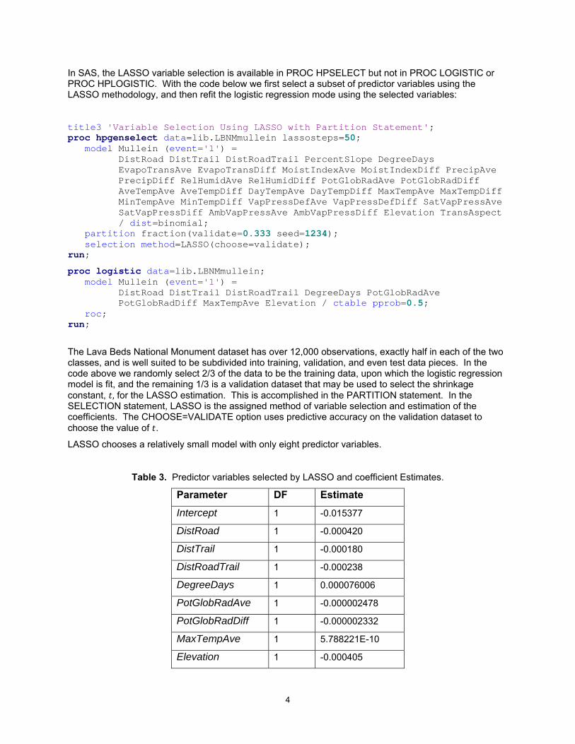
In SAS, the LASSO variable selection is available in PROC HPSELECT but not in PROC LOGISTIC or PROC HPLOGISTIC. With the code below we first select a subset of predictor variables using the LASSO methodology, and then refit the logistic regression mode using the selected variables:

title3 'Variable Selection Using LASSO with Partition Statement'; proc hpgenselect data=lib.LBNMmullein lassosteps=50; model Mullein (event='1') = DistRoad DistTrail DistRoadTrail PercentSlope DegreeDays EvapoTransAve EvapoTransDiff MoistIndexAve MoistIndexDiff PrecipAve PrecipDiff RelHumidAve RelHumidDiff PotGlobRadAve PotGlobRadDiff AveTempAve AveTempDiff DayTempAve DayTempDiff MaxTempAve MaxTempDiff MinTempAve MinTempDiff VapPressDefAve VapPressDefDiff SatVapPressAve SatVapPressDiff AmbVapPressAve AmbVapPressDiff Elevation TransAspect / dist=binomial; partition fraction(validate=0.333 seed=1234); selection method=LASSO(choose=validate); run;

proc logistic data=lib.LBNMmullein; model Mullein (event='1') = DistRoad DistTrail DistRoadTrail DegreeDays PotGlobRadAve PotGlobRadDiff MaxTempAve Elevation / ctable pprob=0.5; roc; run;

The Lava Beds National Monument dataset has over 12,000 observations, exactly half in each of the two classes, and is well suited to be subdivided into training, validation, and even test data pieces. In the code above we randomly select 2/3 of the data to be the training data, upon which the logistic regression model is fit, and the remaining 1/3 is a validation dataset that may be used to select the shrinkage constant, , for the LASSO estimation. This is accomplished in the PARTITION statement. In the SELECTION statement, LASSO is the assigned method of variable selection and estimation of the coefficients. The CHOOSE=VALIDATE option uses predictive accuracy on the validation dataset to choose the value of .

LASSO chooses a relatively small model with only eight predictor variables.

Table 3. Predictor variables selected by LASSO and coefficient Estimates.

Parameter DF Estimate

Intercept 1 -0.015377

DistRoad 1 -0.000420

DistTrail 1 -0.000180

DistRoadTrail 1 -0.000238

DegreeDays 1 0.000076006

PotGlobRadAve 1 -0.000002478

PotGlobRadDiff 1 -0.000002332

MaxTempAve 1 5.788221E-10

Elevation 1 -0.000405

5

The three variables that contain the distances to the nearest roads and trails all have negative coefficients indicating the probability of finding the invasive mullein decreases as the distance from roads and trails increase, which is completely consistent with the published literature on invasive species. This model sacrifices some predictive accuracy for model simplification. The model with just eight variables selected by LASSO trades off some predictive accuracy for model simplification: the accuracy estimates in Table 4 below are slightly lower than for the logistic regression model with all the predictor variables and for the logistic regression model with 15 predictors selected by backward elimination.

Table 4. Accuracy of logistic regression model using 8 predictor variables selected by LASSO.

Percent Correct Sensitivity Specificity

73.8% 75.3% 72.3%

1.2 CLASSIFICATION TREES

Classification trees (Breiman et al., 1984) are one of the earliest machine leaning alternatives to logistic regression and remain popular because of ease of interpretation, natural segmentation of the space of the predictor variables, and accuracy in situations where there are complex interactions among the predictor variables. Loh (2002, 2007) has shown that single classification trees with judiciously chosen variable splits can be nearly as accurate as much more complicated and difficult to interpret ensemble classifiers. In SAS classification trees (and regression trees) may be fit in PROC HPSPLIT, which has recently been added to SAS® STAT™.

Classification and regression trees work by recursive partitioning of the data into groups (“nodes”) that are increasingly homogeneous with respect to some kind of a criterion, such as mean squared error for regression trees and either entropy or the Gini index for classification trees. Ultimately the fitted tree is “pruned” back to remove branches and leaves of the tree that are just fitting noise in the data. The pruning process is a critical part of fitting a classification tree: unpruned trees overfit the data and are less accurate predictors for new data. The approach of segmenting the data space is quite different to that of fitting linear, quadratic or additive functions to the predictor variables. In cases where there are strong interactions among predictor variables, classification trees can outperform linear and quasi linear methods.

The first step in the fitting of a classification tree is to determine the appropriate size of the fitted tree. The code below addresses this issue:

proc hpsplit data=lib.LBNMmullein cvmethod=random(10) seed=123 cvmodelfit intervalbins=5000 plots=all maxdepth=25; class Mullein; model Mullein (event='1') = DistRoad DistTrail DistRoadTrail PercentSlope DegreeDays EvapoTransAve EvapoTransDiff MoistIndexAve MoistIndexDiff PrecipAve PrecipDiff RelHumidAve RelHumidDiff PotGlobRadAve PotGlobRadDiff AveTempAve AveTempDiff DayTempAve DayTempDiff MaxTempAve MaxTempDiff MinTempAve MinTempDiff VapPressDefAve VapPressDefDiff SatVapPressAve SatVapPressDiff AmbVapPressAve AmbVapPressDiff Elevation TransAspect; grow gini; prune costcomplexity; run;

6

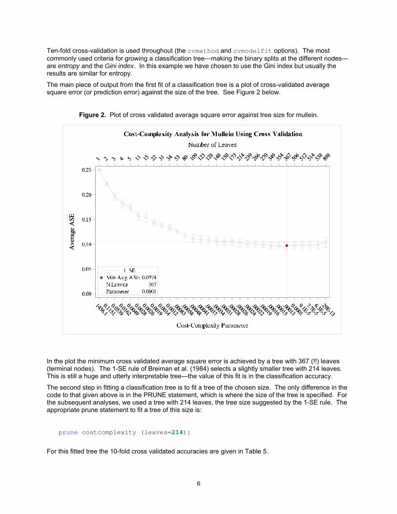
Ten-fold cross-validation is used throughout (the cvmethod and cvmodelfit options). The most commonly used criteria for growing a classification tree—making the binary splits at the different nodes—are entropy and the Gini index. In this example we have chosen to use the Gini index but usually the results are similar for entropy.

The main piece of output from the first fit of a classification tree is a plot of cross-validated average square error (or prediction error) against the size of the tree. See Figure 2 below.

Figure 2. Plot of cross validated average square error against tree size for mullein.

In the plot the minimum cross validated average square error is achieved by a tree with 367 (!!) leaves (terminal nodes). The 1-SE rule of Breiman et al. (1984) selects a slightly smaller tree with 214 leaves. This is still a huge and utterly interpretable tree—the value of this fit is in the classification accuracy.

The second step in fitting a classification tree is to fit a tree of the chosen size. The only difference in the code to that given above is in the PRUNE statement, which is where the size of the tree is specified. For the subsequent analyses, we used a tree with 214 leaves, the tree size suggested by the 1-SE rule. The appropriate prune statement to fit a tree of this size is:

prune costcomplexity (leaves=214);

For this fitted tree the 10-fold cross validated accuracies are given in Table 5.

1 2 3 4 5 11 15 22 31 34 53 80 109

123

128

148

150

173

214

239

266

270

349

354

367

506

512

514

538

898

Ave

rage

ASE

1456.1

0.1151

0.0539

0.0162

0.0049

0.0028

0.0026

0.0019

0.0014

0.0012

.00083

.00058

.00048

.00041

.00037

.00034

.00031

.00028

.00026

.00024

.00022

.00019

.00016

.00015

.00013

0.0001

9.1E-5

7.7E-5

6.3E-5

29E-13

1 2 3 4 5 11 15 22 31 34 53 80 109

123

128

148

150

173

214

239

266

270

349

354

367

506

512

514

538

898

Ave

rage

ASE

1456.1

0.1151

0.0539

0.0162

0.0049

0.0028

0.0026

0.0019

0.0014

0.0012

.00083

.00058

.00048

.00041

.00037

.00034

.00031

.00028

.00026

.00024

.00022

.00019

.00016

.00015

.00013

0.0001

9.1E-5

7.7E-5

6.3E-5

29E-13

7

Table 5. Accuracy of classification tree with 214 leaves (terminal nodes).

Percent Correct Sensitivity Specificity

87.4% 89.9% 85.0%

These accuracies are quite a bit better than for any of the logistic regression model. The 10% increase in accuracy corresponds to about a 45% relative decrease in error. The downside of the fitted classification tree is that it is too large to be interpreted in a meaningful way.

1.3 RANDOM FORESTS

Random Forests (Breiman, 2001) takes predictions from many classification or regression trees and combines them to construct more accurate predictions. The basic algorithm is as follows:

1. Many random samples are drawn from the original dataset. Observations in the original dataset that are not in a particular random sample are said to be out-of-bag for that sample.

2. To each random sample a classification or regression tree is fit without any pruning.

3. The fitted tree is used to make predictions for all the observations that are out-of-bag for the sample the tree is fit to.

4. For a given observations, the predictions from the trees on all of the samples for which the observation was out-of-bag are combined. In regression this is accomplished by averaging the out-of-bag predictions; in classification it is achieved by “voting” the out-of-bag predictions, so the class that is predicted by the largest number of trees for which the observation is out-of-bag is the overall predicted value for that observation.

Many details are omitted from the discussion here, including the number of samples to be drawn from the original data, the size of those samples, whether the samples are drawn with or without replacement, and the number of variables available for the binary partitioning in each tree and at each node. In truth, Random Forests is remarkably robust to choices of all these elements.

Random Forests may be fit using the HPFOREST procedure in SAS® Enterprise Miner™. Here is some sample code for the Lava Beds National Monument data:

proc hpforest data=lib.LBNMmullein maxtrees=500 scoreprole=oob; input DistRoad DistTrail DistRoadTrail PercentSlope DegreeDays EvapoTransAve EvapoTransDiff MoistIndexAve MoistIndexDiff PrecipAve PrecipDiff RelHumidAve RelHumidDiff PotGlobRadAve PotGlobRadDiff AveTempAve AveTempDiff DayTempAve DayTempDiff MaxTempAve MaxTempDiff MinTempAve MinTempDiff VapPressDefAve VapPressDefDiff SatVapPressAve SatVapPressDiff AmbVapPressAve AmbVapPressDiff Elevation TransAspect / level=interval; target Mullein / level=nominal; ID Mullein; score out=LBNMForestsPred; run; proc freq data=LBNMForestsPred; tables Mullein*I_Mullein F_Mullein*I_Mullein / nocol; run;

8

The syntax is a little different from SAS STAT procedures. In particular, predictor (explanatory) variables are specified through INPUT statements. Interval valued and nominal predictor variables must be specified in separate INPUT statements. The response variable is specified in the TARGET statement. For the Lava Beds data, the response variable, MULLEIN, is coded as 1 if mullein is present at the sire and 0 if it is not. Without any further qualification, PROC HPFOREST assumes that such a variable is numerical and would fit a regression forest. To get PROC HPFOREST to fit a classification forest we specify level=nominal or level=binary in the TARGET statement. The SCORE statement computes predicted values for each observation in the original dataset. In order to make sure that the predicted values are computed using only the out-of-bag predictions, we must specify scoreprole=oob in the PROC HPFOREST statement. In the sample code we have set the number of trees to be fitted (which is the number or random samples to be drawn from the data) to be equal to 500 with the maxtrees=500 option. This is massive overkill: 100 trees (the default in PROC HPFOREST) would be plenty for these data and most other data. PROC HPFOREST fits trees so quickly and efficiently it is tempting to fit many more trees than are needed “just in case” there is an increasing trend in accuracy with the number of trees fitted.

The accuracy results for PROC HPFOREST applied to the Lava Beds National Monument data are given in Table 6 below.

Table 6. Accuracy of Random Forests classification applied to the Lava Beds data.

Percent Correct Sensitivity Specificity

93.5% 97.4% 89.6%

The only way to describe these results is “spectacular!” These figures are higher than for the classification tree with 214 nodes and much higher than for any logistic regression models. Indeed, the overall error rate for Random Forests is 6.5% (100% Percent Correct), for the classification tree it is almost twice as high at 12.6%, and for all of the logistic regression models the overall error rate is over 22%. The very high classification accuracy of Random Forests in this problem is not an artifact of overfitting: if we fully cross validate the prediction estimates from PROC HPFOREST we obtain essentially the same accuracies. Gradient boosting machines (Friedman, 2001) yield predictions of comparable accuracy on these data. The analyses in this example illustrate a very important issue, namely that for certain problems machine/statistical learning methods can produce much more accurate predictions than traditional methods for the same goal.

2. MACHINE/STATISTICAL LEARNING METHODS FOR INTERPRETATION

In the previous section we saw that machine learning methods, both old (e.g., classification trees) and new (e.g., Random Forests) can be very more accurate for prediction that traditional methods such as logistic regression. A criticism that is frequently levelled at machine/statistical learning methods is that they are “black boxes” and it is really hard to understand how the methods are fitting the data and the high accuracy is achieved. In part this criticism is fair—machine/statistical learning methods are very algorithmic and are generally not model based in the sense that multiple linear regression, logistic regression, and even generalized additive models are. Graphical tools such as partial dependence plots (Friedman, 2001) address this head on, providing graphical representations of the relationships between individual or pairs of predictors and an interval or binary response variables. In Random Forests, a matrix of “similarities” of observations may be examined graphically using multidimensional scaling. In situations in which small classification trees adequately fit data they can provide some very natural insights as to the form of the classification function.

9

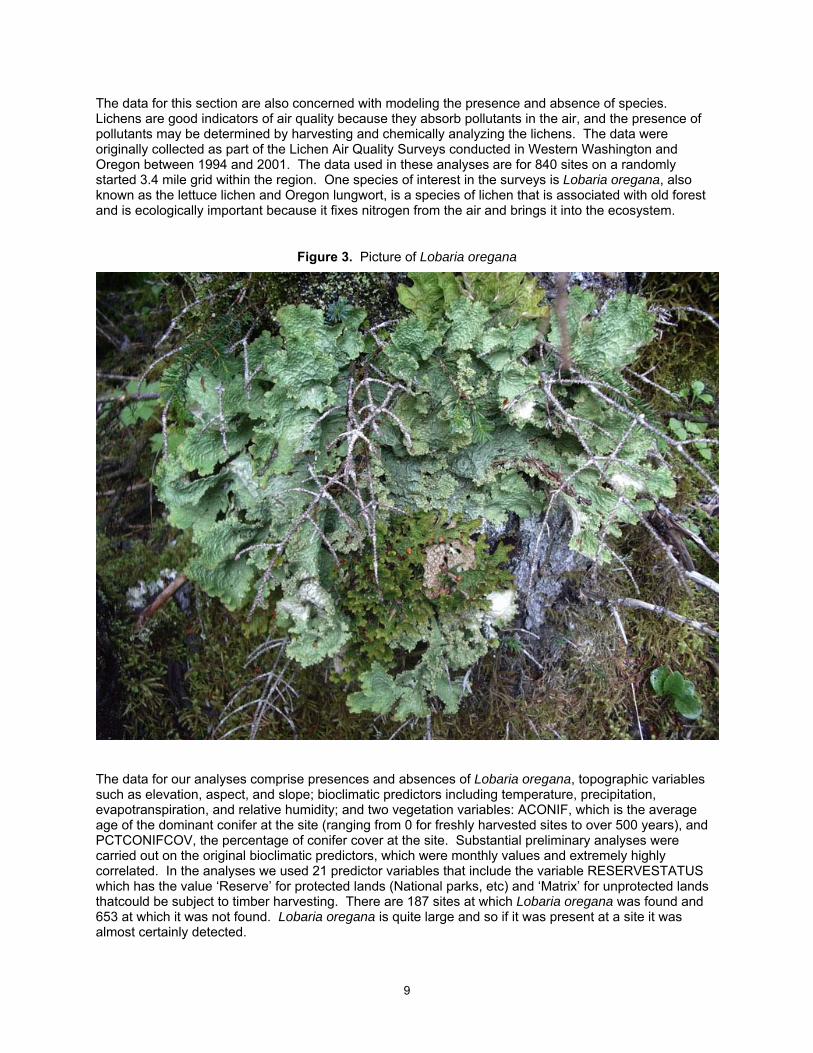
The data for this section are also concerned with modeling the presence and absence of species. Lichens are good indicators of air quality because they absorb pollutants in the air, and the presence of pollutants may be determined by harvesting and chemically analyzing the lichens. The data were originally collected as part of the Lichen Air Quality Surveys conducted in Western Washington and Oregon between 1994 and 2001. The data used in these analyses are for 840 sites on a randomly started 3.4 mile grid within the region. One species of interest in the surveys is Lobaria oregana, also known as the lettuce lichen and Oregon lungwort, is a species of lichen that is associated with old forest and is ecologically important because it fixes nitrogen from the air and brings it into the ecosystem.

Figure 3. Picture of Lobaria oregana

The data for our analyses comprise presences and absences of Lobaria oregana, topographic variables such as elevation, aspect, and slope; bioclimatic predictors including temperature, precipitation, evapotranspiration, and relative humidity; and two vegetation variables: ACONIF, which is the average age of the dominant conifer at the site (ranging from 0 for freshly harvested sites to over 500 years), and PCTCONIFCOV, the percentage of conifer cover at the site. Substantial preliminary analyses were carried out on the original bioclimatic predictors, which were monthly values and extremely highly correlated. In the analyses we used 21 predictor variables that include the variable RESERVESTATUS which has the value ‘Reserve’ for protected lands (National parks, etc) and ‘Matrix’ for unprotected lands thatcould be subject to timber harvesting. There are 187 sites at which Lobaria oregana was found and 653 at which it was not found. Lobaria oregana is quite large and so if it was present at a site it was almost certainly detected.

10

As with the Lava Beds National Monument data in Section 1.2, the initial fit in PROC HPSPLIT is to determine the appropriate tree size. From this we obtained the following cross validated average square error plot as a function of tree size.

Figure 4. Plot of cross validated average square error against tree size for Lobaria oregana.

The minimum average square error is for a tree with 10 leaves (terminal nodes), but the 1-SE rule of Breiman et al. (1984) selects a much smaller model with just 4 leaves.

The code blow is for fitting this smaller model to the Lichen Air Quality data in PROC HPSPLIT.

proc hpsplit data=LAQI cvmethod=random(10) seed=123 cvmodelfit plots=all; class LobaOreg ReserveStatus; model LobaOreg (event='1') = TransAspect Elevation Slope ACONIF PctConifCov DegreeDays EvapoTransAve EvapoTransDiff MoistIndexAve MoistIndexDiff PrecipAve PrecipDiff RelHumidAve RelHumidDiff TempAve TempDiff VapPressAve VapPressDiff PotGlobRadAve PotGlobRadDiff ReserveStatus; grow gini; prune costcomplexity (leaves=4); run;

Ten-fold cross validation is used to evaluate the accuracy of the model.

Ave

rage

ASE

Ave

rage

ASE

11

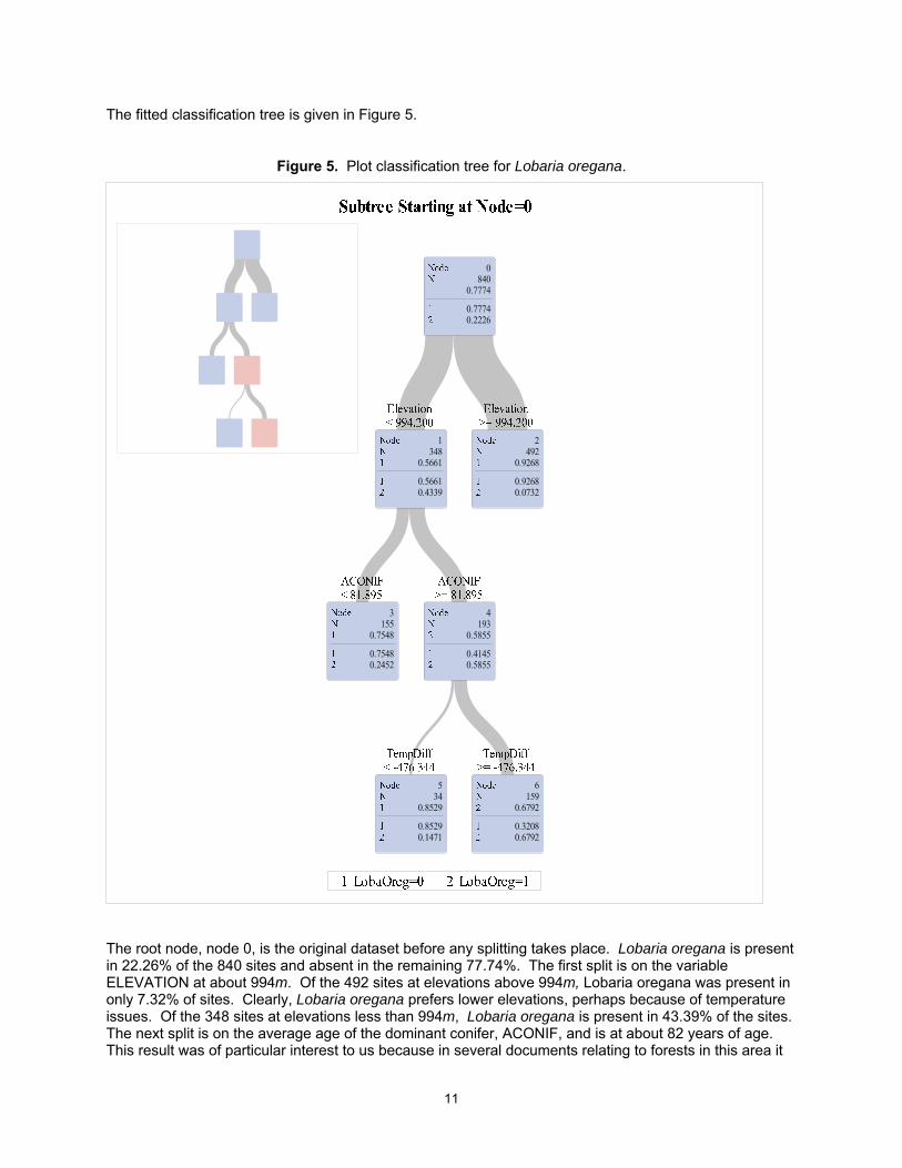
The fitted classification tree is given in Figure 5.

Figure 5. Plot classification tree for Lobaria oregana.

The root node, node 0, is the original dataset before any splitting takes place. Lobaria oregana is present in 22.26% of the 840 sites and absent in the remaining 77.74%. The first split is on the variable ELEVATION at about 994m. Of the 492 sites at elevations above 994m, Lobaria oregana was present in only 7.32% of sites. Clearly, Lobaria oregana prefers lower elevations, perhaps because of temperature issues. Of the 348 sites at elevations less than 994m, Lobaria oregana is present in 43.39% of the sites. The next split is on the average age of the dominant conifer, ACONIF, and is at about 82 years of age. This result was of particular interest to us because in several documents relating to forests in this area it

12

was stated that forests in the pacific Northwest begin to exhibit old forest characteristics at about 80 years of age—and Lobaria oregana is an old forest associated lichen. For the sites for which ACONIF was greater than 81.895 (and for which ELEVATION is less than 994m), Lobaria oregana is present in 58.55%--more than half—of the sites. Splitting on additional variables increases the proportion of sites at which Lobaria oregana is present for some of the nodes to greater than 2/3.

The interpretation of this tree was very straightforward. One could explain the tree to someone with very little technical background and we have done so to middle and high school science students. This is a level of interpretability that exceeds even commonly used parametric methods such as logistic regression.

How well does the classification tree with four leaves fit or predict the data compared to other approaches? Logistic regression was carried out with and without variable selection. The accuracy of the respective methods are summarized in Table 7 below.

Table 7. Accuracy of classification tree with 4 terminal nodes and logistic regression for predicting the presence of Lobaria oregana in the Lichen Air Quality Surveys.

Method Percent Correct Sensitivity Specificity

Classification Tree 83.4% 57.8% 91.0%

Logistic Regression 84.2% 58.8% 91.4%

The accuracies are almost identical across the board. The classification tree that divides the dataset into 4 subgroups is just as accurate a classifier as logistic regression models with 8 or more predictor variables. The classification tree has an additional benefit in that it automatically generates strata for future sampling efforts.

CONCLUSION

In this paper, through examples we have examined some of the issues concerning machine/statistical learning methods. We would like to suggest the following conclusions.

1. With powerful software, like SAS, applying machine/statistical learning methods to the analysis of data is really no more difficult than carrying out multiple regression with variable selection, logistic regression, discriminant analysis.

2. The emphasis when applying machine/statistical learning methods is generally more on prediction rather than explanation and inference. Indeed, with very large datasets traditional hypothesis testing and constructing of confidence intervals becomes meaningless, and the emphasis is necessarily on prediction and identification of variables that are important for obtaining accurate predictions.

3. In some problems machine/statistical learning methods are much more accurate predictors than traditional methods. For the mullein data from Lava Beds National Monument a classification tree (albeit a big one) provided substantially more accurate predictions than logistic regression models and Random Forests, a more sophisticated ensemble classifier, yielded spectacularly accurate predictions.

4. Machine/statistical learning approaches, including the simpler ones such as classification trees, can provide some different but very interesting insights into the structure of the data. The example of the lichen species Lobaria oregana in the Pacific Northwest was a case in which a very simple tree with 4 leaves fit the data well and was easily interpreted in the context of the data.

13

For all these reasons, and many others, machine/statistical learning methods are an important elements of the modern statistician’s toolkit and we should embrace this methodology and figure out ways of using it more effectively to analyze data.

REFERENCES

Breiman, Leo, Jerome Friedman, Richard Olshen, and Charles Stone. 1984. Classification and Regression Trees. Boca Raton, FL: Chapman & Hall.

Breiman, Leo. 2001. “Random Forests.” Machine Learning 45(1):5--32.

Cortes, Corinna and Vladmir Vapnik. 1995. “Support-vector Networks.” Machine Learning 20:273—297.

Cutler, Richard, Thomas Edwards Jr., Karen Beard, Adele Cutler, Kyle Hess, Jacob Gibson, and Joshua Lawler. 2007. “Random Forests for Classification in Ecology.” Ecology 88(11):2783—2792.

Freund, Yoav. 1995. “Boosting a weak learning algorithm by majority.” Information and Computation 121(2):256–285.

Friedman, Jerome. 2001. “Greedy Function Approximation: The Gradient Boosting Machine.” Annals of Statistics 29(5):1189—1232.

Freund, Yoav and Robert Schapire. 1997. “A decision-theoretic generalization of on-line learning and an application to boosting.” Journal of Computer and System Sciences 55(1):119–139.

Loh, Wei-Yin. (2002). “Regression Trees with Unbiased Variable Selection and Interaction Detection.” Statistica Sinica 12:361—386.

Loh, Wei-Yin. (2009). “Improving the Precision of Classification Trees.” Annals of Applied Statistics 3:1710—1737.

Stone, Mervyn. 1974. “Cross-validatory Choice and Assessment of Statistical Predictions.” JRSS B 36(2):111—147.

Tibshirani, Robert. 1996. “Regression Shrinkage and Selection via the LASSO.” JRSS B 58(1):267—288.

Vapnik, Vladmir. 1995. The Nature of Statistical Learning Theory. New York, NY: Springer-Verlag, Inc.

Zou, Hui and Trevor Hastie. 2007. “Regularization and Variable Selection Via the Elastic Net.” JRSS B 67(2):301—332.

CONTACT INFORMATION

Your comments and questions are valued and encouraged. Contact the author at:

Richard Cutler Department of Mathematics and Statistics Utah State University Richard.Cutler@usu.edu