0
What is the best environmental policy? Taxes, permits and rules
under economic and environmental uncertainty
by
Konstantinos Angelopoulos+, George Economides# and Apostolis Philippopoulos* ±
April 30, 2010
Abstract: We welfare rank different types of second-best environmental policy. The focus is on the roles of uncertainty and public finance. The setup is the basic stochastic neoclassical growth model augmented with the assumptions that pollution occurs as a by-product of output produced and environmental quality is treated as a public good. To compare different policy regimes, we compute the welfare-maximizing value of the second-best policy instrument in each regime. In all cases studied, pollution permits are the worst recipe, even when their revenues are used to finance public abatement. When the main source of uncertainty is economic, the best recipe is to levy taxes (on pollution or output) and use the collected tax revenues to finance public abatement. However, when environmental uncertainty is the dominant source of extrinsic uncertainty, Kyoto-like rules for emissions, being combined with tax-financed public abatement, are better than taxes. Finally, comparing pollution and output taxes, the latter are better. Keywords: General equilibrium; uncertainty; environmental policy. JEL classification: C68; D81; H23.
+ University of Glasgow. # Athens University of Economics and Business. * Athens University of Economics and Business; University of Glasgow; CESifo, Munich. ± Corresponding author: Apostolis Philippopoulos, Department of Economics, Athens University of Economics and Business, 76 Patission street, Athens 10434, Greece. Tel: 0030-210-8203357. Fax: 0030-210-8203301. Email: [email protected] Acknowledgements: We thank Nick Hanley, Saqib Jafarey, Jim Malley, Elissaios Papyrakis, Hyun Park , Vangelis Vassilatos and Tassos Xepapadeas for comments and discussions. Any errors are ours.
1
1. Introduction
Environmental degradation caused by human activities is a main concern worldwide.
When economic agents do not internalize the effects of their actions on the
environment, there is need for government intervention to enact appropriate policies
that deal with the negative externalities of pollution emissions. Policy intervention can
take many forms. It is thus useful to be able to rank alternative environmental policies
according to certain criteria, so that the society can choose the best one (in dynamic
models, see e.g. Stokey, 1988, and Jones and Manuelli, 2001).
Examples of environmental policy instruments include taxes, permits (also
known as cap-and-trade policy) and numerical targets for cutting emissions (also
known as command-and-control policy). All of them are distorting and thus second-
best. In the case of taxes, for instance, taxes on pollution itself or on pollution-
generating output, the government raises the price of economic activities. In the case
of permits, the government creates a market for pollution, by issuing a number of
permits, and firms pollute as much as they wish only to the extent that they pay the
price. In the case of numerical targets, the government sets an emission standard
directly so that firms have to restrict their production accordingly and/or make
particular technology and fuel choices. Although this list is not exhaustive,1 there has
always been a lot of interest in the relative desirability of these three policy
instruments, in terms of economic performance, environmental quality and social
welfare (see e.g. Stokey, 1998, section 6).
Two issues are particularly important to the debate on the choice of the
appropriate policy instrument. The first issue has to do with the size and source of
uncertainty. In assessing the risks from climate change and the costs of averting it,
there is a variety of uncertainties that contribute to big differences of opinion as to
how, and how much, to limit emissions (on uncertainty and the environment, see e.g.
the Congressional Budget Office paper prepared for the Congress of the US, 2005).
The second issue refers to the public finance requirements of environmental
protection. It is recognized that the more ambitious is the environmental policy, the
1 For other policy instruments, see e.g. Goulder et al. (1999) and Bovenberg and Goulder (2002).

2
higher the finance requirements for adaptation and mitigation actions,2 and public
finance should play a key role in meeting these requirements (on finance and the
environment, see e.g. the Communication from the European Commission, 2009).3
In this paper, we study the roles of uncertainty and public finance in the
welfare ranking of different types of environmental policy in a micro-founded
dynamic stochastic general equilibrium model. Motivated by the above, we focus on
the following policy regimes: We first model the case in which the government levies
taxes either on pollution itself or on output, and uses the collected tax revenues to
finance public abatement activities. Second, we study the case in which public
abatement activities are financed by the sale of auctioned pollution permits. Third, we
study the case in which environmental policy takes the form of binding numerical rules
à la Kyoto, which specify the speed to a long-term pollution target over time.4
Our setup is a basic stochastic neoclassical growth model augmented with the
assumptions that pollution occurs as a by-product of output produced and
environmental quality has a public good character. Within this setup, there is reason
for policy intervention. There are two exogenous stochastic processes that create
uncertainty about future outcomes and drive the stochastic dynamics of the model. The
first is uncertainty about production technology (standard shocks to total factor
productivity) and the second arises from uncertainty about the impact of economic
activity on the environment.5 Loosely speaking, we call the former shock “economic”
and the latter “environmental”.
We study the implications of the above policy regimes (taxes, permits and
rules) for macroeconomic outcomes, environmental quality and, ultimately, social
welfare. The latter is defined as the conditional expectation of the discounted sum of
household’s lifetime utility. Since the equilibrium solution in each regime depends on
2 According to the European Commission’s estimates, finance requirements could reach 100 billion euros per year by 2020 in developing countries only (see the Communication from the European Commission, 2009). 3 Governments undertake a lot of environmental protection activities (known as public abatement). Examples include policies that protect, conserve and generate (via innovation) the natural resources, as well as policies that provide the right environmental incentives. All these are costly activities that require public funds. Actually, the proportion of public expenditure in total expenditure on abatement is high in most countries (see e.g. Hatzipanayotou et al., 2003, and Haibara, 2009). 4 An example is the reduction of emissions by 25-40% compared to 1990 levels by 2020. Such rules were a key part of the Kyoto protocol designed in 1997 and continue to be a debated issue (see the Copenhagen UN Conference in December 2009). 5 Future trends in emissions are uncertain depending on the pace of economic growth, the demand for fossil fuel, the development of technologies, etc (see e.g. the Congressional Budget Office paper prepared for the Congress of the US, 2005).

3
the values of the second-best policy instruments employed, we welfare rank the
alternative policy regimes when the policy instruments under each regime take their
welfare-maximizing values. We focus on flat over time policy instruments (see also
e.g. Stokey and Rebelo, 1995). To solve the model and compute the associated
welfare under each policy regime, we approximate both the equilibrium solution and
the welfare criterion to second-order around their non-stochastic long-run; in
particular, we use the methodology of Schmitt-Grohé and Uribe (2004).
Our results are as follows. First, public abatement activities constitute an
important part of environmental policy. Policies that yield no pollution revenues, and
do not allow for public abatement, suffer a disadvantage relative to revenue-yielding
policies like taxes and auctioned permits.6 In our setting, without being combined
with public abatement policy, pure Kyoto-like rules cannot be comparable to taxes
and permits and, at least for a wide range of parameter values, such rules are clearly
inferior to taxes and permits. Hence, to make the comparison of alternative regimes
meaningful when we move to a stochastic setup, instead of studying pure rules, we
study mixed rules which combine (in the long run only) rules with public abatement
policy financed by, say, output taxes. Now, when second-best policy instruments take
their welfare-maximizing values, and we are in a deterministic setup, all policy
regimes are equivalent and give the same welfare. This is as in Weitzman (1974).
Second, when we move to an uncertain world, permits are clearly the worst
regime. They may help to fix environmental quality at a relatively high level, but only
at the cost of exposing this quality to exogenous shocks/variability and damaging
private consumption. Actually, the higher the extrinsic (economic or environmental)
uncertainty, the worse is the disadvantage of permits relative to taxes and mixed rules.
This holds for a wide range of parameters, shocks and relative variances of different
categories of shocks. This happens because permits are a hybrid of price- and
quantity-based regulations.7 As a price-based instrument, they are less closely
connected to the heart of the market failure (pollution externality) than taxes. At the
6 This presupposes that any revenues from pollution taxes or auctioned permits are earmarked for the financing of public abatement. This is a conventional notion in the literature. See e.g. Haibara (2009). See also Auerbach (2010) who uses the term “dedicated taxes” to describe the case in which sources and uses of government funds are related. 7 As explained by Bovenberg and Goulder (2002, p. 1520), they are price-based because market forces determine the price of permits. On the other hand, they are quantity-based because the government sets the total amount of permits and emissions. See below for details.
4
same time, as a quantity-based instrument, they provide less controllability than
numerical rules that command agents to produce or emit at a certain level.
Third, in an uncertain world, the verdict of (pollution and output) taxes versus
mixed rules is open depending on the relative variances of different categories of
shocks affecting the economy. The main advantage of mixed rules over taxes is that
they reduce environmental volatility. But this is achieved at the cost of more volatile
consumption. When extrinsic uncertainty arises from economic sources, the latter
effect dominates and hence taxes are preferable to rules. However, when
environmental uncertainty is the dominant source, the former effect dominates and so
rules are preferable. To further analyze this finding, we examine the first and second
moments of those endogenous variables that shape social welfare under each policy
regime and each level of uncertainty. Rules to produce a certain level of output enjoy
an efficiency advantage when environmental uncertainty is high and so the marginal
benefits from nature protection are big. By contrast, when environmental uncertainty
is relatively low, it is better to name a tax and let private agents find the optimal
quantities themselves; in this case, policies like rules for emissions, which reduce the
number of choices that private agents can make, hurt the economy. This intuition is
consistent with Weitzman’s (1974, pp. 485-6) interpretation when he compares price
vs quantity controls in a static framework.8
Fourth, again in an uncertain world, when the comparison is between pollution
taxes and output taxes, the latter are better. The attractiveness of output taxes gets
bigger when environmental uncertainty is high. This result is due to the automatic
stabilizing role of taxation. In particular, the tax base available to the government
under output taxes is larger than under pollution taxes. Hence, under non-internalized
market externalities, macroeconomic volatility is higher under pollution taxes and this
hurts welfare.
The rest of the paper is organized as follows. The next section explains how
we differ from the literature. Sections 3, 4 and 5 solve for taxes, permits and rules
respectively. The first-best is in section 6. The key section is section 7 that compares
welfare across regimes. Section 8 closes the paper. An appendix includes details.
8 Note that “prices” and “quantities” in Weitzman (1974) are closer to pollution taxes and pollution permits respectively in our setup. It is, thus, interesting that taxes are always found to be better than

5
2. How we differ from the literature
Our work is the first attempt to welfare-rank pollution taxes, output taxes, auctioned
pollution permits and numerical rules for emissions in a unified micro-founded
dynamic stochastic general equilibrium (DSGE) model, by paying particular attention
to the source of uncertainty faced. Our work also differs because we allow the
government to play a mix of roles (to correct for externalities, to raise funds to finance
public abatement and to shield the economy from shocks) that are important in the
policy debate. Finally, we look not only at the final welfare effects, but also at the
various channels through which extrinsic uncertainty shapes welfare and, in
particular, we look at the first and second moments of endogenous economic and
environmental variables.
In his seminal work, Weitzman (1974) compared price- and quantity-based
regulations showing that uncertainty causes otherwise equivalent policies to produce
different results. Weitzman focused on the case in which the regulator is uncertain
about the marginal cost and benefit of pollution and (as Bovenberg and Goulder,
2002, p. 1530, and Schöb, 1996, point out) worked in a first-best setting, in the sense
that regulation did not distort private decisions. Since then there has been a rich and
still expanding literature on the comparison of alternative policy instruments in the
presence of uncertainty. However, in most of these papers, the approach has been
static and/or partial equilibrium, and the comparison is between taxes and quotas only
(see the survey by Bovenberg and Goulders, 2002, section 4.2). An exception is Pizer
(1999) who used a DSGE model. However, here we use a second-order
approximation to both the equilibrium solution and the welfare criterion (Pizer used a
first-order approximation to the equilibrium solution). This is important because it
allows us to take into account the uncertainty that the agents face when making
decisions. Also, as shown by Rotemberg and Woodford (1997), Woodford (2003,
chapter 6), Schmitt-Grohé and Uribe (2004, 2007) and many others, a second-order
approximation to the model’s equilibrium solution, as well as to the welfare function,
helps us to avoid potential spurious welfare rankings of various regimes that may
arise when the model’s equilibrium solution is approximate to first-order only (see
permits (at least in the numerical specifications we have used), while the source and magnitude of extrinsic uncertainty becomes important to policy ranking only when we compare taxes to rules.
6
section 7 below for further details). Finally, Pizer (1999) compared “rate controls”
with taxes only and did not allow for public abatement.
Finally, it is worth stressing that the previous environmental literature has not
examined the importance of the source of extrinsic uncertainty for the choice of
efficient policies; as we find, this is crucial. In addition, the literature has not
considered public abatement together with pollution regulation.9 Finally, none of the
previous studies has studied numerical rules for emissions.
3. A model with taxes
We augment the basic stochastic neoclassical growth model with natural resources
and environmental policy. The economy is populated by a large number of identical
infinitely-lived private agents that derive utility from private consumption and the
stock of environmental quality. Private agents consume, save and produce a single
good. Output produced generates pollution and this damages environmental quality.
Since private agents take economy-wide environmental quality as a public good, i.e.
they do not internalize the effects of their actions on the environment, the
decentralized equilibrium is inefficient. Hence, there is room for government
intervention.
In this section, government intervention takes the form of taxes. We focus on
two types of taxes: first, taxes on output, where output is the polluting activity in our
model; second, taxes on pollution itself. Whatever the type of taxation, any collected tax
revenues are used to finance public abatement policy. Since output taxes are the most
common policy instrument in the related growth literature (see e.g. Xepapadeas, 2004,
and Economides and Philippopoulos, 2008), we start with them.
Private agents
For simplicity, the population size is constant and equal to one. The private agent’s
expected utility is defined over stochastic sequences of private consumption, tc , and
the economy’s beginning-of-period environmental quality, tQ :
9 Schöb (1996), Goulder et al. (1999) and Bovenberg and Goulder (2002, section 4.1), among many others, have also emphasized the public-finance aspect of environmental policies. But they focus on the so-called revenue recycling effect or the double-dividend effect, which means that funds so raised can
7
00
( , )tt t
t
E u c Qβ∞
=∑ (1a)
where 10 << β is a time preference rate and 0E is an expectations operator based on
the information available at time zero.
Without loss of generality, we use for instantaneous utility:
1 1[( ) ( ) ]( , )
1t t
t tc Qu c Q
μ μ σ
σ
− −
=−
(1b)
where 0 ,1 1μ μ< − < are the weights given to consumption and environmental
quality respectively and 1σ ≥ is a measure of risk aversion.
The private agent’s within-period budget constraint is:
1 (1 ) (1 ) (1 )kt t t t t t t tk k c y A kαδ τ τ+ − − + = − = − (2)
where t t ty A kα= is current output,10 1+tk is the end-of-period capital stock, tk is the
beginning-of-period capital stock, tA is a standard index of production technology
(whose stochastic motion is defined below), 10 << α and 0 1kδ≤ ≤ are usual
parameters, and 10 <≤ tτ is the tax rate on (polluting) output.
The agent chooses 1 0{ , }t t tc k ∞+ = to maximize (1a-b) subject to (2) taking policy
variables and environmental quality as given. The latter is justified by the open-access
and public-good features of the environment.
Natural resources
The stock of environmental quality evolves over time according to:11
1 (1 )q qt t t tQ Q Q p gδ δ ν+ = − + − + (3)
be used to reduce other taxes. Baldursson et al. (2008) focus on the time-consistency of various environmental policy instruments. 10 We abstract from labor-leisure choices to keep the model simpler. We report that this is not important qualitatively.
8
where 0Q ≥ represents environmental quality without pollution, tp is the current
pollution flow, tg is public spending on abatement activities, and 0 1qδ≤ ≤ and
0ν ≥ are parameters measuring respectively the degree of environmental persistence
and how public spending is translated into actual units of renewable natural resources.
The flow of pollution, tp , is modeled as a by-product of output produced, ty :
t t t t t tp y A kαφ φ= = (4)
where tφ is an index of pollution technology or a measure of emissions per unit of
output.12 We assume that tφ is stochastic (its motion is defined below).
Government budget constraint
Assuming a balanced budget for the government, we have in each period:
t t t t t tg y A kατ τ= = (5)
where tg is public spending on abatement policy.
Exogenous stochastic variables
We assume that the two technologies, tA and tφ , follow (1)AR stochastic processes
of the form:
1(1 )1
aa a t
t tA A A eρ ρ ε +−+ = (6a)
1(1 )1
tt t e
φφ φρ ρ εφ φ φ +−
+ = (6b)
where A and φ are constants, 0 , 1a φρ ρ< < are auto-regressive parameters and
,at t
φε ε are Gaussian i.i.d. shocks with zero means and known variances, 2aσ and 2
φσ .
11 The motion of natural resources in (3) is as in Jouvet et al. (2005); see p. 1599 in their paper for further details. The inclusion of the parameter 0Q ≥ is helpful when we solve the model numerically. 12 One could assume that pollution technology has also an endogenous component depending on e.g. private and public investment in pollution-reducing technology.

9
Decentralized competitive equilibrium (given output taxes)
The Decentralized Competitive Equilibrium (DCE) of the above economy is
summarized by the following equations at 0t ≥ (see Appendix A.1 for details):
1 (1 ) (1 )kt t t t t tk k c A kαδ τ+ − − + = − (7a)
111 1 1
1
[1 (1 ) ]kt tt t t t
t t
u uE A kc c
αβ δ τ α −++ + +
+
⎡ ⎤∂ ∂= − + −⎢ ⎥∂ ∂⎣ ⎦
(7b)
1 (1 ) ( )q qt t t t t tQ Q Q A kαδ δ φ ντ+ = − + − − (7c)
where (1 ) 1 (1 )(1 )( ) ( )tt t
t
u c Qc
μ σ μ σμ − − − −∂=
∂. This is a three-equation system in
1 1 0{ , , }t t t tc k Q ∞+ + = . This DCE is for given policy (where the latter is summarized by
output tax rates 0{ }t tτ ∞= levied by the government), initial conditions for the stock
variables, 0k and 0Q , and stochastic processes for the exogenous variables, tA and
tφ . Section 7 will choose the output tax rate.
Decentralized competitive equilibrium (given pollution taxes)
When there are taxes on pollution itself rather than on polluting activities like output,
the DCE is summarized by the following equations at 0t ≥ (see Appendix A.3 for
details):
1 (1 ) (1 )kt t t t t t tk k c A kαδ φ θ+ − − + = − (8a)
111 1 1 1
1
[1 (1 ) ]kt tt t t t t
t t
u uE A k
c cαβ δ φ θ α −+
+ + + ++
⎡ ⎤∂ ∂= − + −⎢ ⎥∂ ∂⎣ ⎦
(8b)
1 (1 ) ( )q qt t t t t t tQ Q Q A kαδ δ φ νφ θ+ = − + − − (8c)
We thus have a new three-equation system in 1 1 0{ , , }t t t tc k Q ∞+ + = . This DCE is for given
policy (where the latter is summarized by pollution tax rates 0{ }t tθ ∞= levied by the
10
government), initial conditions, 0k and 0Q , and stochastic processes, tA and tφ .
Section 7 will choose the pollution tax rate.13
4. The same model with permits
Now the government creates a market for pollution by issuing a number of permits that
matches its maximum target amount of pollution. In order to pollute legally, a private
agent has to hold a number of permits equal to its own quantity of pollution. In turn, the
government uses the collected revenues to finance public abatement policy. The model
in this section is similar to that used by Jouvet et al. (2005).14
In particular, we assume that, at each time t , the government issues a quantity
of pollution permits, tP , and auctions them at a price, tq . These permits are bought in
the current period but can be used by the polluting private agent/firm in the next time
period, 1t + .15 Thus, the private agent’s budget constraint changes from (2) to:
1 1(1 )kt t t t t t t tk k c q p y A kαδ+ +− − + + = = (9)
where 1 1 1 1 1 1t t t t t tp y A kαφ φ+ + + + + += = .
The government budget constraint changes from equation (5) to:
t t tg q P= (10)
13 The special case in which the government uses taxes to internalize externalities only (Pigouvian case) is in Appendix A.2. 14 Jouvet et al. (2005) focus on whether permits should be given away rather than sold by the government. 15 In this model specification, we cannot assume that permits are bought and used in the same current period. This is because current-period pollution is given (see Appendix B.4, where the right-hand side of equation (B.5d) consists of exogenous and predetermined variables only, implying that tP cannot be a policy control variable). This applies to the transition path; by contrast, it is not a problem in the long run (see Appendix B.4 for details). Allowing, for instance, for endogenous labor could allow permits to be bought and used within the same period but it would complicate the model unnecessarily. As we report below when we study the long run, even quantitative results are affected very little by this timing assumption. In any case, it is worth noting that our assumed timing (namely, that permits are bought today but are used in the next period) is close to the recent Obama climate-change bill, where the

11
Decentralized competitive equilibrium (given the quantity of pollution permits)
The DCE of the above economy is summarized by the following equations at 0t ≥
(see Appendix B.1 for details):16
11 (1 )k t
t t t t tt
Pk k c q Pδφ−
+ − − + + = (11a)
1 111 1 1 1 1
1
(1 [ ]) [ (1 )]kt tt t t t t t t t
t t
u uq E A k E A kc c
α αα φ β δ α− −++ + + + +
+
∂ ∂+ = − +
∂ ∂ (11b)
1 1(1 )q qt t t t tQ Q Q P q Pδ δ ν+ −= − + − + (11c)
1 1 1 1[ ]t t t t t t tP E p E A kαφ+ + + += = (11d)
We thus have a four-equation system in 1 1 0{ , , , }t t t t tc k Q q ∞+ + = . This new DCE is for
given policy - where the latter is summarized by the quantity of pollution permits
0{ }t tP ∞= issued by the government - initial conditions, 0k and 0Q , and stochastic
processes, tA and tφ . Section 7 will choose the quantity of pollution permits.17
5. The same model with numerical rules for emissions
We next study the case in which the government specifies the speed to a long-term
pollution target. By speed, we mean that pollution tomorrow will be a fraction of
pollution today, where this fraction is part of environmental policy. This approach can
be captured by a policy rule like:
tttt ppp γγ +−=+ )1(1 (12)
where p is long-run pollution and 0 1tγ< ≤ is an autoregressive “parameter”.
government issues a fixed number of permits to emit carbon dioxide each year, which firms must buy before releasing their stuff into the atmosphere (see e.g. The Economist, July 4, 2009, p. 37). 16 Equation (11d) is a market-clearing condition which states that, in equilibrium, agents’ demand for pollution equals supply with the latter determined by the government. See also Jouvet et al. (2005). 17 The special case in which the government uses permits to internalize externalities only is in Appendix B.2. Appendix B.3 shows the case in which the government sets the price of permits allowing their quantity to be market determined.
12
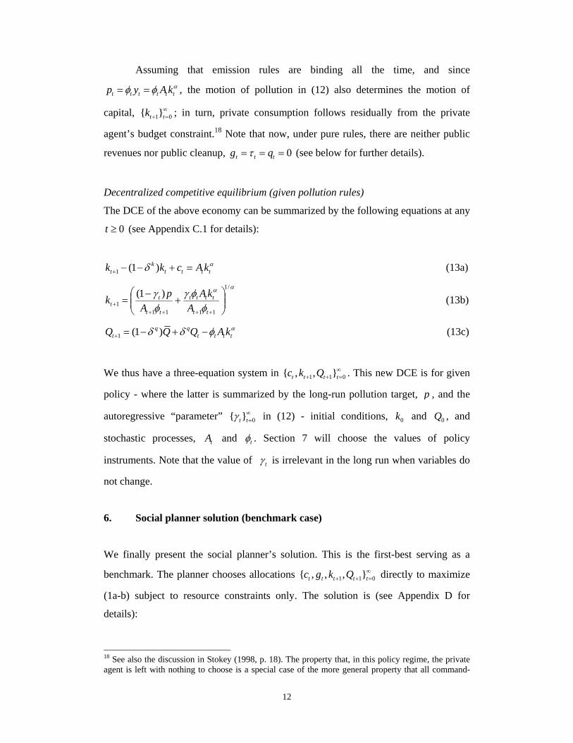
Assuming that emission rules are binding all the time, and since
t t t t t tp y A kαφ φ= = , the motion of pollution in (12) also determines the motion of
capital, 1 0{ }t tk ∞+ = ; in turn, private consumption follows residually from the private
agent’s budget constraint.18 Note that now, under pure rules, there are neither public
revenues nor public cleanup, 0t t tg qτ= = = (see below for further details).
Decentralized competitive equilibrium (given pollution rules)
The DCE of the above economy can be summarized by the following equations at any
0t ≥ (see Appendix C.1 for details):
1 (1 )kt t t t tk k c A kαδ+ − − + = (13a)
αα
φφγ
φγ
/1
11111
)1(⎟⎟⎠
⎞⎜⎜⎝
⎛+
−=
+++++
tt
tttt
tt
tt A
kAA
pk (13b)
1 (1 )q qt t t t tQ Q Q A kαδ δ φ+ = − + − (13c)
We thus have a three-equation system in 1 1 0{ , , }t t t tc k Q ∞+ + = . This new DCE is for given
policy - where the latter is summarized by the long-run pollution target, p , and the
autoregressive “parameter” 0{ }t tγ ∞= in (12) - initial conditions, 0k and 0Q , and
stochastic processes, tA and tφ . Section 7 will choose the values of policy
instruments. Note that the value of tγ is irrelevant in the long run when variables do
not change.
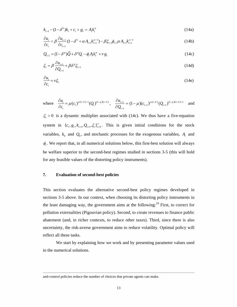
6. Social planner solution (benchmark case)
We finally present the social planner’s solution. This is the first-best serving as a
benchmark. The planner chooses allocations 1 1 0{ , , , }t t t t tc g k Q ∞+ + = directly to maximize
(1a-b) subject to resource constraints only. The solution is (see Appendix D for
details):
18 See also the discussion in Stokey (1998, p. 18). The property that, in this policy regime, the private agent is left with nothing to choose is a special case of the more general property that all command-
13
1 (1 )kt t t t t tk k c g A kαδ+ − − + + = (14a)
1 111 1 1 1 1 1
1
(1 )kt tt t t t t t
t t
u u A k A kc c
α αβ δ α βξ φ α− −++ + + + + +
+
∂ ∂= − + −
∂ ∂ (14b)
1 (1 )q qt t t t t tQ Q Q A k gαδ δ φ ν+ = − + − + (14c)
11
1
qtt t
t
uQ
ξ β βδ ξ++
+
∂= +
∂ (14d)
tt
t
uc
νξ∂=
∂ (14e)
where (1 ) 1 (1 )(1 )( ) ( )tt t
t
u c Qc
μ σ μ σμ − − − −∂=
∂, (1 ) (1 )(1 ) 11
1 11
(1 )( ) ( )tt t
t
uc Q
Qμ σ μ σμ − − − −+
+ ++
∂= −
∂ and
0tξ > is a dynamic multiplier associated with (14c). We thus have a five-equation
system in 1 1 0{ , , , , }t t t t t tc g k Q ξ ∞+ + = . This is given initial conditions for the stock
variables, 0k and 0Q , and stochastic processes for the exogenous variables, tA and
tφ . We report that, in all numerical solutions below, this first-best solution will always
be welfare superior to the second-best regimes studied in sections 3-5 (this will hold
for any feasible values of the distorting policy instruments).
7. Evaluation of second-best policies
This section evaluates the alternative second-best policy regimes developed in
sections 3-5 above. In our context, when choosing its distorting policy instruments in
the least damaging way, the government aims at the following:19 First, to correct for
pollution externalities (Pigouvian policy). Second, to create revenues to finance public
abatement (and, in richer contexts, to reduce other taxes). Third, since there is also
uncertainty, the risk-averse government aims to reduce volatility. Optimal policy will
reflect all these tasks.
We start by explaining how we work and by presenting parameter values used
in the numerical solutions.
and-control policies reduce the number of choices that private agents can make.
14
How we work
Since the DCE solution and the resulting welfare, under each policy regime, depend
on the values of the second-best policy instruments employed, we will compare the
maximum welfare across regimes, namely, the welfare resulting from the welfare-
maximizing values of the policy instruments in each regime. Welfare is defined as the
conditional expectation of the discounted sum of household’s lifetime utility. We
focus on flat policy instruments, namely, policy instruments that remain constant over
time (see also e.g. Stokey and Rebelo, 1995, and Ortigueira, 1998). In all cases
reported, there is a tradeoff in policy and hence a well-defined welfare-maximizing
value of policy instruments.
To solve the system of non-linear expected difference equations that form the
DCE in each regime, we approximate both the DCE solution and the welfare criterion
to second-order around the associated non-stochastic steady state solution. We then
compute welfare for a wide range of values of the flat policy instrument in each
regime and thus find the welfare maximizing-value of the policy instrument and the
associated maximum welfare under that regime.20
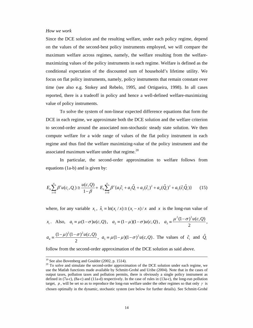
In particular, the second-order approximation to welfare follows from
equations (1a-b) and is given by:
00
( , )( , )1
tt t
t
u c QE u c Qββ
∞
=
≅ +−∑ 2 2
0 1 2 3 4 50
ˆ ˆ ˆˆ ˆ ˆ{ ( ) ( ) ( )}tt t t t t t
t
E a c a Q a c a Q a c Qβ∞
=
+ + + +∑ (15)
where, for any variable tx , ˆ ln( / ) ( ) /t t tx x x x x x≡ ≅ − and x is the long-run value of
tx . Also, 1 (1 ) ( , )a u c Qμ σ≡ − , 2 (1 )(1 ) ( , )a u c Qμ σ≡ − − , 2 2
3(1 ) ( , )
2u c Qa μ σ−
≡ ,
2 2
4(1 ) (1 ) ( , )
2u c Qa μ σ− −
≡ , 25 (1 )(1 ) ( , )a u c Qμ μ σ≡ − − . The values of tc and ˆ
tQ
follow from the second-order approximation of the DCE solution as said above. 19 See also Bovenberg and Goulder (2002, p. 1514). 20 To solve and simulate the second-order approximation of the DCE solution under each regime, we use the Matlab functions made available by Schmitt-Grohé and Uribe (2004). Note that in the cases of output taxes, pollution taxes and pollution permits, there is obviously a single policy instrument as defined in (7a-c), (8a-c) and (11a-d) respectively. In the case of rules in (13a-c), the long-run pollution target, p , will be set so as to reproduce the long-run welfare under the other regimes so that only γ is chosen optimally in the dynamic, stochastic system (see below for further details). See Schmitt-Grohé
15
Finally, we need a measure of comparison of welfare gains/losses associated
with alternative regimes. This measure, denoted as ijζ in what follows, is obtained by
computing the percentage compensation in private consumption that the private agent
would require in each time-period under regime j so as to be equally well off
between regimes i and j i≠ (see the notes in Table 3 for the value of ijζ ). This is a
popular measure in dynamic general equilibrium models (see e.g. Lucas, 1990).
Parameter values
We keep all parameter values the same across different regimes, so that the evaluation
of different policies is not blurred by parameter differences. Whenever parameter
values are important for the results obtained, we will explicitly discuss their effects
and robustness. As said above, the policy instrument in each regime is chosen to
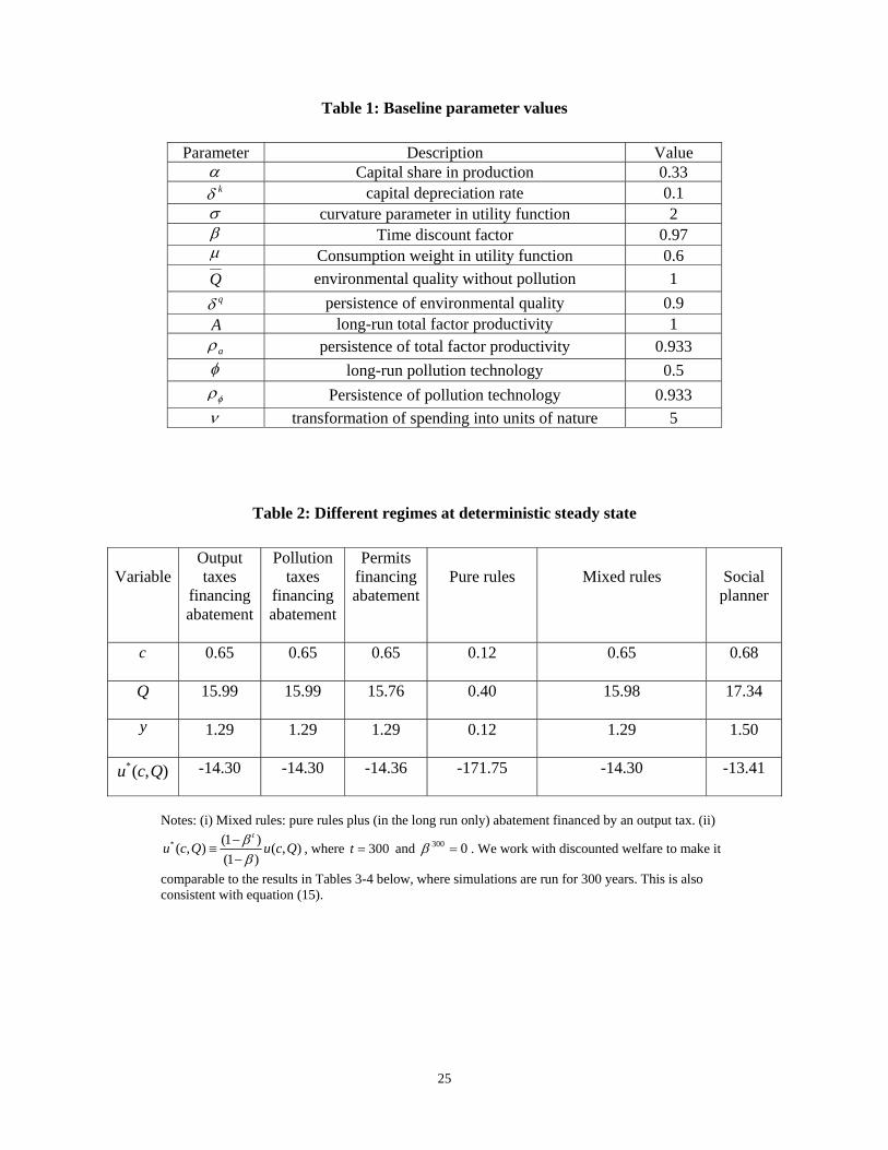
maximize welfare. The parameter values used are reported in Table 1.
Table 1 around here
The values of the economic parameters are rather standard. In particular, the
baseline values used for the rate of time preference ( β ), the depreciation rate of
capital ( kδ ), the capital share in output (α ), the intertemporal elasticity of
substitution ( σ/1 ), the constant term ( A ) and the persistence parameter ( aρ ) of the
TFP process, are as in most dynamic stochastic general equilibrium calibration and
estimation studies. As discussed earlier, we will experiment with different values of
the standard deviation of the TFP process ( aσ ).
There is, of course, much less empirical evidence and consensus on the value
of environmental parameters. For our baseline results, we set μ (i.e. the weight given
to private consumption vis-à-vis environmental quality in the utility function) at a
relatively low level, 0.6, and discuss other results later on. Regarding the parameters
characterizing the exogenous process for environmental technology, we choose a high
persistence parameter, 933.0== αφ ρρ , and normalize its constant term, φ , at 0.5.
Finally, we set v (i.e. how public abatement spending is translated into actual units of
and Uribe (2005) and Kollmann (2008) on how this type of optimally computed policy differs from optimal policy in the Ramsey sense.
16
environmental quality) at 5; this parameter value helps us to match the units in the
environmental quality equation (3) and hence obtain a well-defined trade-off in
second-best policy. Since v is the same across regimes with public abatement
spending (taxes and permits), its value does not matter for the comparison of these
two regimes. Nevertheless, it can matter when we compare these two regimes to the
command-and-control regime which does not allow for public abatement spending
(we discuss this issue below).
We are now ready to present numerical results. Before investigating the
relatively general case in which exogenous shocks cause fluctuations around steady
state, we study the deterministic steady state. This will help us to understand the
working of the model and how results change when uncertainty is introduced. We will
report results for some key variables as well as for the associated welfare.
Evaluation of regimes at steady state (certainty)
We first present results when the economy remains at its non-stochastic steady state.
Steady-state results for consumption, c , environmental quality, Q , output, y , as well
as the resulting welfare, defined as *( , )u c Q , under each regime, are reported in Table
2 (policy instruments are set at their welfare-maximizing values).
Table 2 around here
The second column in Table 2 presents long-run results for the model in
equations (7a-c), where the government sets output taxes and uses the collected tax
revenues to finance its abatement policy. In the third column, the policy instrument is
pollution taxes (see the model in equations (8a-c)). The fourth column presents results
for the model is equations (11a-d), where the government sets the quantity of
pollution permits and finances its abatement policy from the sale of those permits. In
the fifth column, we present results for the model in equations (13a-c), where the
government uses numerical rules; in contrast to previous regimes, now there are no
revenues and hence no abatement policy on the side of the government. The very last
column reports the social planner solution in equations (14a-e); this gives the best
outcome as expected (from now on, we do not study this first-best case).
17
Output taxes, pollution taxes and pollution permits (see second, third and
fourth column in Table 2) are equivalent.21 On the other hand, rules (see fifth column)
clearly differ from taxes and permits. In particular, using our baseline parameter
values, Kyoto-like rules appear to be much worse than both taxes and permits. In
general, however, this welfare comparison is ambiguous depending on parameter
values.22 This finding arises simply because pure rules are not really comparable to
the other two regimes: in our setting, by assumption, such rules do not generate public
revenues and hence do not allow for public abatement policy (or, more generally,
given tax bases, they allow for less public abatement policy than revenue-raising
regimes like taxes and permits). Thus, to get a meaningful comparison of different
regimes when we introduce uncertainty below, we have to make them equivalent in a
deterministic setup. We therefore add public abatement policy financed by, say, an
output tax into the regime of pure Kyoto-like rules (see Appendix C.3 for details).
Specifically, we choose the long-run pollution target and the long-run output tax rate
so as to reproduce the same long-run solutions for consumption and environmental
quality, and thus the same long-run welfare, as in the other second-best regimes.
Results are reported in the sixth, second from the end, column in Table 2. In what
follows, instead of pure rules, we will work with this mixed regime – Kyoto-like rules
combined (in the long run only) with public abatement financed by taxes – and
compare this regime to taxes and permits. All policy regimes are now equivalent in a
deterministic setup (see also Table 3 below); this respects Weitzman (1974).
To summarize, there are two policy messages. First, public abatement
activities constitute an important part of environmental policy. Policies that yield no
revenues, and hence do not allow for public abatement, suffer a disadvantage relative
21 In the results for the deterministic steady state in Table 2, any second, or higher, decimal point differences are due to numerical solution approximations of the welfare-maximizing value of policy instruments. In addition, in the case of permits, any differences from the other regimes are due to the assumed timing, namely, permits are bought in the current period but are used in the next period (see also footnote 15 and Appendix B.4). In any case, these differences are quantitatively very small and do not affect our conclusions. 22 Specifically, our comparative static exercises imply that rules are welfare inferior to taxes and permits in the long run, when 0ν ≥ (which measures how public spending on cleanup is translated into actual units of nature) is relatively high and/or 0 1μ< < (which is the weight given to private consumption vis-à-vis environmental quality) is relatively low. Intuitively, when public abatement policy, being financed by tax or permit revenues, is effective in preserving the environment (i.e. when ν is high) and/or we value little the distorting effects of taxes and permits on private consumption (i.e. when μ is low), numerical rules are inferior to taxes and permits. As ν gets smaller and/or μ gets larger, this inferiority diminishes. For very low values of ν and/or very high values of μ , numerical rules can turn out to be welfare superior to taxes and permits.

18
to revenue-yielding policies. This of course presupposes that any revenues from
pollution taxes or permits are earmarked for the financing of public abatement. In this
literature, the key role of public finance has already been pointed out, although the
emphasis has been on the revenue recycling effect (see e.g. Bovenberg and Goulder,
2002, section 4.1). In our model, without being combined with public abatement
policy, pure Kyoto-like rules are not really comparable to taxes and permits and, at
least for a wide range of parameter values used, such rules are inferior to taxes and
permits, especially in terms of environmental quality. Second, to the extent that policy
instruments are chosen optimally, and there is no uncertainty, the choice of the
second-best policy instrument is irrelevant to social welfare. Of course, this can apply
to regimes that are comparable (in our case, all of them allow for abatement policy).
Evaluation of regimes under uncertainty
We now allow for uncertainty coming from the exogenous stochastic autoregressive
processes for production and pollution technologies in equations (6a-b). We suppose
that the economy is initially at its steady state studied above and, starting from 0t = ,
there are shocks to tA and tφ .
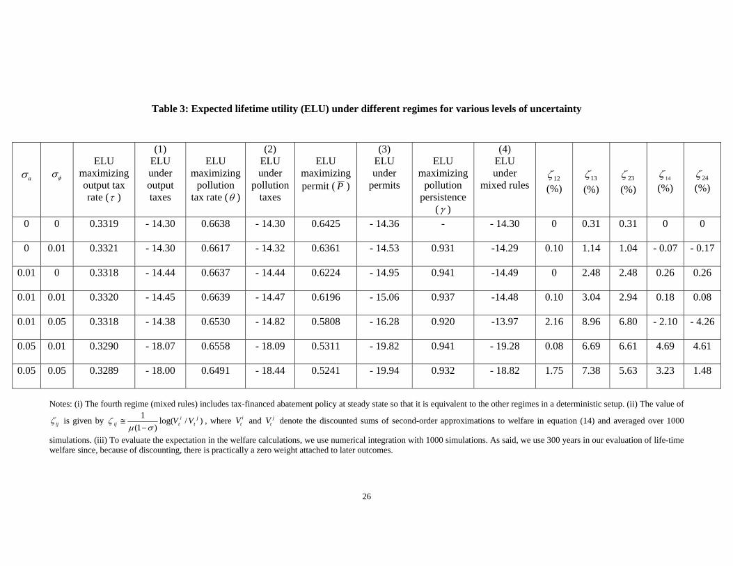
Working as explained above and using the same baseline parameter values, we
compute discounted expected lifetime utility under each regime for a varying degree
of uncertainty as summarized by the standard deviations of production and pollution
technologies, aσ and φσ . Results are reported in Table 3. For expositional reasons,
we study: (i) the deterministic case ( 0a φσ σ= = ); (ii) when there is only one source
of uncertainty ( 01.0=ασ and 0=φσ ; 0=ασ and 01.0=φσ ); (iii) a case of
relatively low uncertainty in both stochastic variables ( 0.01α φσ σ= = ); (iv) two
scenarios representing high levels of uncertainty in one of the two stochastic variables
( 01.0=ασ and 0.05φσ = ; and 0.05ασ = , 01.0=φσ ); (v) a scenario with relatively
high uncertainty in both stochastic variables ( 0.05a φσ σ= = ).
Table 3 around here

19
Table 3 confirms that, in a deterministic environment ( 0a φσ σ= = ), all
regimes imply the same welfare. By contrast, in a stochastic setup where , 0a φσ σ > ,
the choice of the policy instrument does matter. Table 3 also reports the welfare
gain/loss (i.e. the value of ijζ ) when we choose regime i instead of regime j i≠ . A
positive value of ijζ means that i is superior to j . For instance, if 0ij xζ = > , an
agent, who happens to be in j , will require a permanent consumption subsidy of %x
to become indifferent between j and i .
Welfare differences between output taxes and pollution taxes are summarized
by the values of 12ζ in Table 3. Output taxes are more attractive and this
attractiveness gets bigger when environmental uncertainty is relatively high. For
instance, when 0.05φσ = and 0.01ασ = , a welfare gain of 2.16%, in terms of private
consumption, can be obtained if we use output, instead of pollution, taxes. As we will
see in the next subsection, this has to do with the automatic stabilizing role of
taxation. The tax base available to the government under output taxes is larger than
under pollution taxes. Hence macroeconomic volatility is higher under pollution taxes
and this is bad for welfare. It is not surprising that the case for output taxes becomes
stronger when environmental uncertainty is high. The reason is that, only under some
market imperfection, larger governments can moderate the effects of external shocks.
In our model, economic shocks are internalized by private agents themselves. By
contrast, environmental shocks are not internalized since environmental quality is
treated as a public good. This is why a large government size can play its automatic
stabilizing role when environmental uncertainty is high. This result is consistent with
the macroeconomic literature, where a mix of rigidities is needed to produce the
negative correlation between government size and output volatility (see e.g. Andrés et
al., 2008).
Welfare differences between output taxes and permits are summarized by the
values of 13ζ , while welfare differences between pollution taxes and permits are
summarized by the values of 23ζ , in Table 3. Both types of taxes are always superior
to permits. For instance, when 0.01α φσ σ= = , a welfare gain of 3.04% is obtained if
we use output taxes instead of permits. The superiority of taxes further increases with
the degree of uncertainty. For instance, when 0.05α φσ σ= = , the gain, from using
20
output taxes instead of permits, rises to 7.38%. Notice that taxes are superior even
when environmental uncertainty is higher than economic uncertainty. Also notice that
these are substantial welfare gains relatively to those found, for instance, in the
literature on the welfare implications of tax reforms (see e.g. Lucas, 1990, who
compares Ramsey to suboptimal tax structures).
We next compare taxes to mixed rules. Welfare differences between output
taxes and mixed rules, and between pollution taxes and mixed rules, are summarized
respectively by the values of 14ζ and 24ζ in the last two columns of Table 3. When
economic uncertainty ( aσ ) is higher than, or equal to, environmental uncertainty
( φσ ), taxes are better than mixed rules. For low levels of uncertainty, such welfare
differences are small, but the higher aσ and φσ become, the higher the superiority of
taxes over rules, as long as a φσ σ≥ . For instance, when 0.05aσ = and 0.01φσ = , the
gain from using output (resp. pollution) taxes is 4.69% (resp. 4.61%), while when
0.05a φσ σ= = , the gain is 3.23% (resp. 1.48%). On the other hand, when
environmental uncertainty is higher than economic uncertainty ( a φσ σ< ), rules are
better than taxes, especially than pollution taxes. For instance, when 0.01aσ = and
0.05φσ = , the welfare gain from switching from output taxes to mixed rules is
2.10%, while the gain from switching from pollution taxes to mixed rules is 4.26%.
Pollution taxes perform worse than output taxes because their automatic stabilizing
effect is smaller, as discussed above.
To summarize, as shown by Weitzman (1974), ex ante uncertainty affects the
choice of the policy instrument. Taxes and mixed rules are substantially better than
permits; this holds over the whole range of parameter values, the sources of
uncertainty, and the size of variances of shocks, that we have experimented with.
Welfare benefits from the use of taxes, instead of permits, can be high for high levels
of uncertainty irrespectively of where this uncertainty comes from. Comparing output
to pollution taxes, the former are better. However, differences between output and
pollution taxes are small relatively to differences between taxes and permits and
between taxes and rules. On the other hand, the comparison between taxes and mixed
rules depends on the relative variances of different categories of shocks. Taxes are
better than rules when economic uncertainty is no smaller than environmental
21
uncertainty. But, when environmental uncertainty is the dominant source of
uncertainty, mixed rules are superior to taxes, especially to pollution taxes that allow
for a relatively small automatic stabilizing effect.
The intuition behind these welfare results will be discussed in the next
subsection that presents means, variances and covariances of the arguments in the
welfare criterion.
Before we move on, we report that we get well-defined values for the welfare-
maximizing policy instrument in each regime (although we realize that numerical
solutions should be treated with caution, these values are within the expected range).
Results are in Table 3. For instance, when 0.01α φσ σ= = , the optimal output tax rate
is found to be 0.33, the optimal pollution tax rate is 0.66, the optimal quantity of
permits is 0.62 and the optimal degree of pollution persistence under mixed rules is
0.94. Notice that, in general, the values of the policy instruments are not
monotonically increasing in the degree of uncertainty. The reason is that policy
intervention comes at a cost, and also, as explained above, stabilization is only one of
the goals of policy.
Looking behind welfare under uncertainty
To understand what is driving the above welfare differences under uncertainty, we
study the first and second moments of the two arguments in the utility function,
namely, private consumption, tc , and the stock of environmental quality, tQ . Note
from the second-order approximation to the welfare function (15) that, in addition to
the steady state values of tc and tQ and their deviations from these steady state
values, what also matters for welfare is the squared deviations and cross-products of
tc and tQ from their steady state values. Given that the steady state solution values
are the same across policy regimes, any welfare differences in the stochastic setup are
driven by differences in expected means, variances and covariances of the series for
tc and tQ (see Appendix E for details).
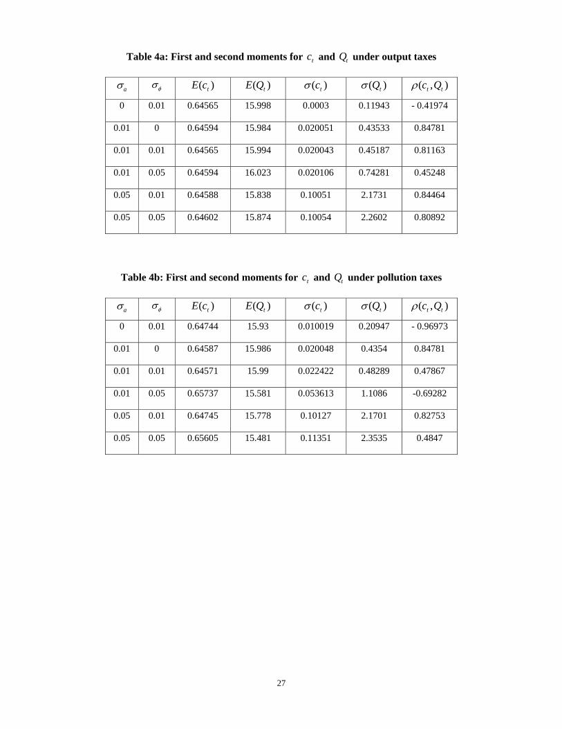
Tables 4a-d present the expected means, standard deviations and correlations
of tc and tQ for all four regimes under various levels of uncertainty. Welfare
increases when the means of tc and tQ increase, their variances decrease and their
correlation decreases.
22
Tables 4a-d around here
As can be seen in Tables 4a-d, different policy regimes imply different trade-
offs in outcomes whose net, total effect on welfare was summarized in Table 3 above.
Some regimes are good for consumption, while others are good for environmental
quality.
In particular, output and emission taxes (see Tables 4a-b) and mixed rules (see
Table 4d) imply higher expected consumption than permits (see Table 4c), while
permits are superior in terms of expected environmental quality, especially when
uncertainty is high. On the other hand, the variance of environmental quality is higher
under permits than under taxes and rules. The higher volatility in environmental
quality, in combination with lower expected consumption, makes permits the worst
regime in all experiments studied. On the other hand, a weak point of taxes is the high
correlation between consumption and environmental quality (by contrast, correlation
is negative in all cases under permits and in most cases under rules, and this is good
for welfare).
The comparison of the two better regimes, taxes and mixed rules in Tables 4a-
b and 4c respectively, implies that the main advantages of mixed rules are that they
reduce environmental variation and also allow consumption deviations to move
counter-cyclically with deviations in environmental quality. For this to be achieved,
however, all the adjustment from an exogenously caused stochasticity has to be
absorbed by consumption. In particular, consumption volatility is higher under rules
than under taxes. When economic uncertainty is no smaller than environmental
uncertainty, as was summarized in Table 3, it is the adverse consumption volatility
effects that dominate so that welfare is higher under taxes.23 But when environmental
uncertainty is the dominant source of uncertainty, the benefits from lower variation in
environmental quality and the inverse correlation between environment and
consumption become important enough to make rules superior to taxes (this happens,
for instance, when 0.01aσ = and 0.05φσ = in Tables 3 and 4).
To summarize, in an uncertain world, permits are the worst regime. They can
fix expected environmental quality at a relatively high level, but only at the cost of
23 This is despite a relatively low value for the weight given to consumption versus environmental quality in the utility function in our calibration (see Table 1). Hence, if anything, our calibration does not do any favours to the tax regime.
23
exposing this expected quality to high volatility and damaging expected private
consumption. The higher the extrinsic uncertainty, the higher is the disadvantage of
permits relative to taxes and mixed rules. This holds for a wide range of parameters,
shocks and relative variances of different categories of shocks. Auctioned permits are
inferior because (as pointed out by Bovenberg and Goulder, 2002, p. 1520) they are a
hybrid of price- and quantity-based regulations. They are price-based because market
forces determine the price of permits. They are quantity-based because the
government sets the total amount of permits and hence emissions. The problem is
that, as a price-based instrument, they are less closely connected to the heart of the
problem (pollution externality) than taxes. At the same time, as a quantity-based
instrument, they provide less controllability than numerical emission rules that
command agents to produce or emit a certain level. This argument is also supported
by the result that when the government uses the price of permits, instead of their
quantity, as a policy instrument (see Appendix B.3), permits and taxes become very
similar on and off steady state (results are available upon request).
The comparison between taxes and mixed rules is open depending on the
relative variances of different categories of shocks affecting the economy. When
uncertainty arises from economic factors, taxes are preferable. But when
environmental uncertainty becomes the dominant source, mixed rules are preferable.
We believe this is consistent with Weitzman’s (1974, pp. 485-6) intuition. As
Weitzman has shown in a first-best setting, quantities are better than prices, as
planning instruments, when the benefit function is more curved and/or the cost
function is more linear. In our model, this seems to be the case under Kyoto-like rules
in the presence of high uncertainty over the environment. In such a situation, better
environmental quality gives a direct welfare benefit to private agents; hence, when
environmental uncertainty is relatively high, the marginal benefits of an extra unit of
natural resources change rapidly and thus the curvature of the benefit function is high.
By contrast, when environmental uncertainty is relatively low, the benefit function is
closer to being linear. In such a situation, prices are a better instrument; the marginal
benefit is almost linear in some range so that it is better to name a price and let private
agents find the optimal quantities themselves. In this case, policies like rules, that
reduce the number of choices that private agents can make, hurt the macro economy.

24
8. Concluding remarks and possible extensions
We evaluated output taxes, pollution taxes, auctioned pollution permits and Kyoto-
like emission rules, in a unified micro-founded dynamic stochastic general
equilibrium model. We focused on the role of uncertainty and showed the importance
of public finance and abatement. The latter is an important ingredient of any
environmental policy. Permits, despite their popularity among politicians, are the
worst regime. When we compare taxes and rules, taxes are better when economic
volatility is the main source of uncertainty. On the other hand, when environmental
shocks are the dominant source of extrinsic uncertainty, rules perform better. Between
taxes, output taxes are better than pollution taxes as a consequence of the small tax
base available to governments taxing only pollution.
We are aware that many issues have not been studied. For instance, it would
be interesting to search for the best international agreement in our setup and, in
particular, the design of international carbon market and international public funding.
It is also important to evaluate environmental policies under structural uncertainty
resulting from model misspecification of the environmental/pollution process. We
leave such issues for future research.
25
Table 1: Baseline parameter values
Parameter Description Value α Capital share in production 0.33
kδ capital depreciation rate 0.1 σ curvature parameter in utility function 2 β Time discount factor 0.97 μ Consumption weight in utility function 0.6 Q environmental quality without pollution 1
qδ persistence of environmental quality 0.9 A long-run total factor productivity 1
aρ persistence of total factor productivity 0.933 φ long-run pollution technology 0.5 φρ Persistence of pollution technology 0.933 ν transformation of spending into units of nature 5
Table 2: Different regimes at deterministic steady state
Variable Output taxes
financing abatement
Pollution taxes
financing abatement
Permits financing abatement
Pure rules
Mixed rules
Social planner
c 0.65
0.65
0.65
0.12
0.65
0.68
Q 15.99
15.99
15.76
0.40 15.98
17.34
y 1.29
1.29
1.29
0.12 1.29
1.50
*( , )u c Q -14.30
-14.30
-14.36
-171.75 -14.30
-13.41
Notes: (i) Mixed rules: pure rules plus (in the long run only) abatement financed by an output tax. (ii)
* (1 )( , ) ( , )(1 )
t
u c Q u c Qββ
−≡
−, where 300t = and 0300 =β . We work with discounted welfare to make it
comparable to the results in Tables 3-4 below, where simulations are run for 300 years. This is also consistent with equation (15).
26
Table 3: Expected lifetime utility (ELU) under different regimes for various levels of uncertainty
Notes: (i) The fourth regime (mixed rules) includes tax-financed abatement policy at steady state so that it is equivalent to the other regimes in a deterministic setup. (ii) The value of
ijζ is given by )/log()1(
1 jt
itij VV
σμζ
−≅ , where i
tV and jtV denote the discounted sums of second-order approximations to welfare in equation (14) and averaged over 1000
simulations. (iii) To evaluate the expectation in the welfare calculations, we use numerical integration with 1000 simulations. As said, we use 300 years in our evaluation of life-time welfare since, because of discounting, there is practically a zero weight attached to later outcomes.
aσ
φσ
ELU
maximizing output tax rate (τ )
(1) ELU under output taxes
ELU
maximizing pollution
tax rate (θ )
(2) ELU under
pollution taxes
ELU
maximizing permit ( P )
(3) ELU under
permits
ELU
maximizing pollution
persistence (γ )
(4) ELU under
mixed rules
12ζ
(%)
13ζ
(%)
23ζ
(%)
14ζ
(%)
24ζ
(%)
0 0 0.3319 - 14.30
0.6638 - 14.30
0.6425 - 14.36
- - 14.30 0 0.31 0.31 0 0
0 0.01 0.3321 - 14.30
0.6617 - 14.32
0.6361 - 14.53
0.931 -14.29 0.10 1.14 1.04 - 0.07 - 0.17
0.01 0 0.3318 - 14.44
0.6637 - 14.44
0.6224 - 14.95
0.941 -14.49 0 2.48 2.48 0.26 0.26
0.01 0.01 0.3320 - 14.45
0.6639 - 14.47
0.6196 - 15.06
0.937 -14.48 0.10 3.04 2.94 0.18 0.08
0.01 0.05 0.3318 - 14.38
0.6530 - 14.82
0.5808 - 16.28
0.920 -13.97 2.16 8.96 6.80 - 2.10 - 4.26
0.05 0.01 0.3290 - 18.07
0.6558 - 18.09
0.5311
- 19.82 0.941 - 19.28 0.08 6.69 6.61 4.69 4.61
0.05 0.05 0.3289 - 18.00
0.6491 - 18.44
0.5241 - 19.94
0.932 - 18.82 1.75 7.38 5.63 3.23 1.48
27
Table 4a: First and second moments for tc and tQ under output taxes
aσ φσ )( tcE )( tQE )( tcσ )( tQσ ),( tt Qcρ
0 0.01 0.64565
15.998
0.0003
0.11943
- 0.41974
0.01 0 0.64594
15.984
0.020051
0.43533
0.84781
0.01 0.01 0.64565
15.994
0.020043
0.45187
0.81163
0.01 0.05 0.64594
16.023
0.020106
0.74281
0.45248
0.05 0.01 0.64588
15.838
0.10051
2.1731
0.84464
0.05 0.05 0.64602
15.874
0.10054
2.2602
0.80892
Table 4b: First and second moments for tc and tQ under pollution taxes
aσ φσ )( tcE )( tQE )( tcσ )( tQσ ),( tt Qcρ
0 0.01 0.64744
15.93
0.010019
0.20947
- 0.96973
0.01 0 0.64587
15.986
0.020048
0.4354
0.84781
0.01 0.01 0.64571
15.99
0.022422
0.48289
0.47867
0.01 0.05 0.65737
15.581
0.053613
1.1086
-0.69282
0.05 0.01 0.64745
15.778
0.10127
2.1701
0.82753
0.05 0.05 0.65605
15.481
0.11351
2.3535
0.4847

28
Table 4c: First and second moments for tc and tQ under permits
aσ φσ )( tcE )( tQE )( tcσ )( tQσ ),( tt Qcρ
0 0.01 0.6361
16.381
0.028102
0.60575
- 0.97038
0.01 0 0.59204
17.661
0.025287
1.5217
- 0.92889
0.01 0.01 0.58519
17.89
0.035702
1.576
- 0.82458
0.01 0.05 0.50656
20.602
0.11027
2.19
- 0.71098
0.05 0.01 0.39463
22.477
0.07966
3.9753
- 0.88201
0.05 0.05 0.39337
22.833
0.11334
4.2228
- 0.61149
Table 4d: First and second moments for tc and tQ under mixed rules
aσ φσ )( tcE )( tQE )( tcσ )( tQσ ),( tt Qcρ
0 0.01 0.6460
15.978
0.0004568
0.11790
0.57035
0.01 0 0.6456
15.980
0.03343
0.13156
- 0.71178
0.01 0.01 0.64588
15.977
0.03342
0.17706
- 0.50837
0.01 0.05 0.65125
15.97095
0.03641
0.54824
0.08256
0.05 0.01 0.64063
15.97728
0.16064
0.66842
- 0.70381
0.05 0.05 0.64475
15.97011
0.16111
0.84335
- 0.49271
29
APPENDICES
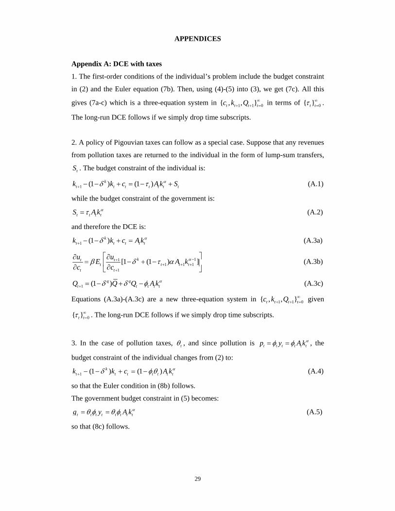
Appendix A: DCE with taxes
1. The first-order conditions of the individual’s problem include the budget constraint
in (2) and the Euler equation (7b). Then, using (4)-(5) into (3), we get (7c). All this
gives (7a-c) which is a three-equation system in 1 1 0{ , , }t t t tc k Q ∞+ + = in terms of 0{ }t tτ ∞
= .
The long-run DCE follows if we simply drop time subscripts.
2. A policy of Pigouvian taxes can follow as a special case. Suppose that any revenues
from pollution taxes are returned to the individual in the form of lump-sum transfers,
tS . The budget constraint of the individual is:
1 (1 ) (1 )kt t t t t t tk k c A k Sαδ τ+ − − + = − + (A.1)
while the budget constraint of the government is:
t t t tS A kατ= (A.2)
and therefore the DCE is:
1 (1 )kt t t t tk k c A kαδ+ − − + = (A.3a)
111 1 1
1
[1 (1 ) ]kt tt t t t
t t
u uE A kc c
αβ δ τ α −++ + +
+
⎡ ⎤∂ ∂= − + −⎢ ⎥∂ ∂⎣ ⎦
(A.3b)
1 (1 )q qt t t t tQ Q Q A kαδ δ φ+ = − + − (A.3c)
Equations (A.3a)-(A.3c) are a new three-equation system in 1 1 0{ , , }t t t tc k Q ∞+ + = given
0{ }t tτ ∞= . The long-run DCE follows if we simply drop time subscripts.
3. In the case of pollution taxes, tθ , and since pollution is t t t t t tp y A kαφ φ= = , the
budget constraint of the individual changes from (2) to:
1 (1 ) (1 )kt t t t t t tk k c A kαδ φ θ+ − − + = − (A.4)
so that the Euler condition in (8b) follows.
The government budget constraint in (5) becomes:
t t t t t t t tg y A kαθ φ θ φ= = (A.5)
so that (8c) follows.
30
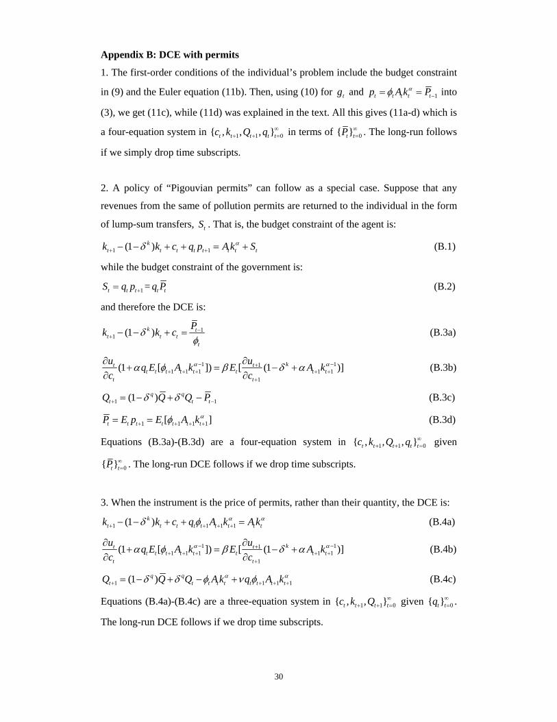
Appendix B: DCE with permits
1. The first-order conditions of the individual’s problem include the budget constraint
in (9) and the Euler equation (11b). Then, using (10) for tg and 1t t t t tp A k Pαφ −= = into
(3), we get (11c), while (11d) was explained in the text. All this gives (11a-d) which is
a four-equation system in 1 1 0{ , , , }t t t t tc k Q q ∞+ + = in terms of 0{ }t tP ∞
= . The long-run follows
if we simply drop time subscripts.
2. A policy of “Pigouvian permits” can follow as a special case. Suppose that any
revenues from the same of pollution permits are returned to the individual in the form
of lump-sum transfers, tS . That is, the budget constraint of the agent is:
1 1(1 )kt t t t t t t tk k c q p A k Sαδ+ +− − + + = + (B.1)
while the budget constraint of the government is:
1t t tS q p += = t tq P (B.2)
and therefore the DCE is:
11 (1 )k t
t t tt
Pk k cδφ−
+ − − + = (B.3a)
1 111 1 1 1 1
1
(1 [ ]) [ (1 )]kt tt t t t t t t t
t t
u uq E A k E A kc c
α αα φ β δ α− −++ + + + +
+
∂ ∂+ = − +
∂ ∂ (B.3b)
1 1(1 )q qt t tQ Q Q Pδ δ+ −= − + − (B.3c)
1 1 1 1[ ]t t t t t t tP E p E A kαφ+ + + += = (B.3d)
Equations (B.3a)-(B.3d) are a four-equation system in 1 1 0{ , , , }t t t t tc k Q q ∞+ + = given
0{ }t tP ∞= . The long-run DCE follows if we drop time subscripts.
3. When the instrument is the price of permits, rather than their quantity, the DCE is:
1 1 1 1(1 )kt t t t t t t t tk k c q A k A kα αδ φ+ + + +− − + + = (B.4a)
1 111 1 1 1 1
1
(1 [ ]) [ (1 )]kt tt t t t t t t t
t t
u uq E A k E A kc c
α αα φ β δ α− −++ + + + +
+
∂ ∂+ = − +
∂ ∂ (B.4b)
1 1 1 1(1 )q qt t t t t t t t tQ Q Q A k q A kα αδ δ φ ν φ+ + + += − + − + (B.4c)
Equations (B.4a)-(B.4c) are a three-equation system in 1 1 0{ , , }t t t tc k Q ∞+ + = given 0{ }t tq ∞
= .
The long-run DCE follows if we drop time subscripts.
31
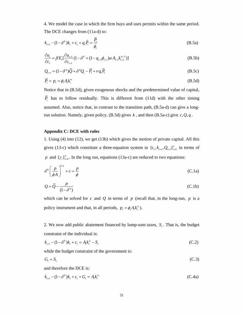
4. We model the case in which the firm buys and uses permits within the same period.
The DCE changes from (11a-d) to:
1 (1 )k tt t t t t
t
Pk k c q Pδφ+ − − + + = (B.5a)
111 1 1 1
1
[ (1 (1 ) )]kt tt t t t t
t t
u uE q A kc c
αβ δ φ α −++ + + +
+
∂ ∂= − + −
∂ ∂ (B.5b)
1 (1 )q qt t t t tQ Q Q P q Pδ δ ν+ = − + − + (B.5c)
t t t t tP p A kαφ= = (B.5d)
Notice that in (B.5d), given exogenous shocks and the predetermined value of capital,
tP has to follow residually. This is different from (11d) with the other timing
assumed. Also, notice that, in contrast to the transition path, (B.5a-d) can give a long-
run solution. Namely, given policy, (B.5d) gives k , and then (B.5a-c) give , ,c Q q .
Appendix C: DCE with rules
1. Using (4) into (12), we get (13b) which gives the motion of private capital. All this
gives (13-c) which constitute a three-equation system in 1 1 0{ , , }t t t tc k Q ∞+ + = in terms of
p and 0{ }t tγ ∞= . In the long run, equations (13a-c) are reduced to two equations:
1/k p pc
A
α
δφ φ⎛ ⎞
+ =⎜ ⎟⎝ ⎠
(C.1a)
(1 )q
pQ Qδ
= −−
(C.1b)
which can be solved for c and Q in terms of p (recall that, in the long-run, p is a
policy instrument and that, in all periods, t t t tp A kαφ= ).
2. We now add public abatement financed by lump-sum taxes, tS . That is, the budget
constraint of the individual is:
1 (1 )kt t t t t tk k c A k Sαδ+ − − + = − (C.2)
while the budget constraint of the government is:
t tG S= (C.3)
and therefore the DCE is:
1 (1 )kt t t t t tk k c G A kαδ+ − − + + = (C.4a)
32
αα
φφγ
φγ
/1
11111
)1(⎟⎟⎠
⎞⎜⎜⎝
⎛+
−=
+++++
tt
tttt
tt
tt A
kAA
pk (C.4b)
1 (1 )q qt t t t t tQ Q Q A k Gαδ δ φ ν+ = − + − + (C.4c)
In the long run, equations (C.4a)-(C.4c) are reduced to two equations: 1/
k p pc GA
α
δφ φ⎛ ⎞
+ + =⎜ ⎟⎝ ⎠
(C.5a)
(1 )q
p GQ Q νδ
−= −
− (C.5b)
which can be solved for c and Q in terms of p and G .
3. We now add public abatement financed by output taxes, tτ . The budget constraint
of the individual is:
1 (1 ) (1 )kt t t t t tk k c A kαδ τ+ − − + = − (C.6)
while the budget constraint of the government is:
t t t tG A kατ= (C.7)
and therefore the DCE is:
1 (1 ) (1 )kt t t t t tk k c A kαδ τ+ − − + = − (C.8a)
αα
φφγ
φγ
/1
11111
)1(⎟⎟⎠
⎞⎜⎜⎝
⎛+
−=
+++++
tt
tttt
tt
tt A
kAA
pk (C.8b)
1 (1 ) ( )q qt t t t t tQ Q Q A kαδ δ φ ντ+ = − + − − (C.8c)
In the long run, equations (C.8a)-(C.8c) are reduced to two equations: 1/
(1 )k p pcA
α
δ τφ φ⎛ ⎞
+ = −⎜ ⎟⎝ ⎠
(C.9a)
1
(1 )q
pQ Q
ντφδ
⎛ ⎞−⎜ ⎟
⎝ ⎠= −−
(C.9b)
which can be solved for c and Q in terms of p and τ . We choose the values of p
and τ so as to hit the long-run solution of the previous regimes.
Appendix D: Social planner’s solution
The planner chooses 1 1 0{ , , , }t t t t tc g k Q ∞+ + = to maximize (1a-b) subject to the resource
constraints:
33
1 (1 )kt t t t t tk k c g A kαδ+ − − + + = (D.1a)
1 (1 )q qt t t t t tQ Q Q A k gαδ δ φ ν+ = − + − + (D.1b)
The optimality conditions include (D.1a), (D.1b) and:
1 111 1 1 1 1 1
1
(1 )kt tt t t t t t
t t
u u A k A kc c
α αβ δ α βξ φ α− −++ + + + + +
+
∂ ∂= − + −
∂ ∂ (D.2a)
11
1
qtt t
t
uQ
ξ β βδ ξ++
+
∂= +
∂ (D.2b)
tt
t
uc
νξ∂=
∂ (D.2c)
where 0>ξ is a dynamic multiplier associated with (D.1b),
(1 ) 1 (1 )(1 )( ) ( )tt t
t
u c Qc
μ σ μ σμ − − − −∂=
∂, and (1 ) (1 )(1 ) 11
1 11
(1 )( ) ( )tt t
t
uc Q
Qμ σ μ σμ − − − −+
+ ++
∂= −
∂. (D.1a)-
(D.1b) and (D.2a)-(D.2c) constitute a five-equation system in { }∞=++ 011 ,,,, tttttt gQkc ξ .
The long-run follows if we drop time subscripts.
Appendix E: Statistical moments
To see that examining the means, variances and covariances of the variables in levels
is equivalent to examining the same moments for the variables defined as deviations
from their (common) steady state, note the following. For the random variables x and
y , define xxx −=ˆ and yyy −=ˆ , where x (resp. y ) is the average value of x
(resp. y ). The relationship between the mean of x and the mean of x is given by:
xxExE −= )()ˆ( (E.1)
(E.1) implies that, when x is the same across regimes, any differences in the mean of
x are due to differences in the mean of x . The relationship between 2x and the
variance of x is given by: 222 )]ˆ([)ˆ()]ˆ(ˆ[)ˆvar( xExExExEx −=−= (E.2)
Hence, given the mean of x , any differences in the average value of 2x are captured
by differences in the variance of x . Further, the variances of x and x are the same,
i.e. )var()])(()[()]ˆ(ˆ[)ˆvar( 22 xxxExxExExEx =−−−=−= . Finally, given their
means, any differences in the cross-products of x and y are captured by their
covariance, i.e. )ˆ()ˆ(]ˆˆ[)ˆ,ˆcov( yExEyxEyx −= , where:
{ } { } ),cov()])(())][()(()[()]ˆ(ˆ)][ˆ(ˆ[)ˆ,ˆcov( yxyyEyyxxExxEyEyxExEyx =−−−−−−=−−= (E.3)

34
References
Andrés J., R. Doménech and A. Fátas (2008): The stabilizing role of government size, Journal of Economic Dynamics and Control, 32, 571-593. Auerbach A. (2010): Public finance in practice and theory, CESifo Economic Studies, 56, 1-20. Baldursson F. M. and N.-H. M. von der Fehr (2008): Prices vs. quantities: public finance and the choice of regulatory instruments, European Economic Review, 52, 1242-1255. Bovenberg A. L. and L. H. Goulder (2002): Environmental taxation and regulation, in Handbook of Public Economics, volume 3, edited by A. Auerbach and M. Feldstein, North-Holland, Amsterdam. Congressional Budget Office (2005): Uncertainty in analyzing climate change: policy implications, The Congress of the United States, Congressional Budget Office Paper, January, Washington. Economides G. and A. Philippopoulos (2008): Growth enhancing policy is the means to sustain the environment, Review of Economic Dynamics, 11, 207-219. European Commission (2009): Stepping up international climate finance: a European blueprint for the Copenhagen deal, COM(2009) 475/3, Commission of the European Communities, Brussels. Goulder L. H., I. W. H. Parry, R. C. Williams III and D. Burtraw (1999): The cost-effectiveness of alternative instruments for environmental protection in a second-best setting, Journal of Public Economics, 72, 329-360. Haibara T. (2009): Environmental funds, public abatement and welfare, Environmental and Resource Economics, 44, 167-177. Hatzipanayotou P., S. Lahiri and M. Michael (2003): Environmental policy reform in a small open economy with public and private abatement, in Environmental Policy in an International Perspective, edited by L. Marsiliani, M. Rauscher and C. Withagen, Kluwer, London. Jones L. and R. Manuelli (2001): Endogenous policy choice: the case of pollution and growth, Review of Economic Dynamics, 4, 369–405. Jouvet P. A., P. Michel and G. Rotillon (2005): Optimal growth with pollution: how to use pollution permits, Journal of Economic Dynamics and Control, 29, 1597-1609. Kollmann R. (2008): Welfare-maximizing operational monetary and tax policy rules, Macroeconomic Dynamics, 12, 112-125. Lucas R. E. (1990): Supply-side economics: an analytical review, Oxford Economic Papers, 42-293-316.
35
Ortigueira S. (1998): Fiscal policy in an endogenous growth model with human capital accumulation, Journal of Monetary Economics, 42, 323-355. Pizer W. (1999): The optimal choice of climate change policy in the presence of uncertainty, Resource and Energy Economics, 21, 255-287. Rotemberg J. and M. Woodford (1997): An optimization-based econometric framework for the evaluation of monetary policy, in NBER Macroeconomics Annual 1997, edited by O. Blanchard and S. Fischer, MIT Press. Schmitt-Grohé S. and M. Uribe (2004): Solving dynamic general equilibrium models using a second-order approximation to the policy function, Journal of Economic Dynamics and Control, 28, 755-775. Schmitt-Grohé S. and M. Uribe (2005): Optimal fiscal and monetary policy in a medium-scale macroeconomic model, in NBER Macroeconomics Annual 2005, edited by G. Gertler and K. Rogoff, MIT Press, 383-425. Schmitt-Grohé S. and M. Uribe (2007): Optimal simple and implementable monetary and fiscal rules, Journal of Monetary Economics, 54, 1702-1725. Schöb R. (1996): Choosing the right instrument: the role of public revenues for environmental policy, Environmental and Resource Economics, 8, 399-416. Stokey N. (1998): Are there limits to growth? International Economic Review, 39, 1-31. Stokey N. and S. Rebelo (1995): Growth effects of flat-rate taxes, Journal of Political Economy, 103, 519-550. Weitzman M. (1974): Prices vs. quantities, Review of Economic Studies, 41, 477-491. Woodford M. (2003): Interest and Prices: Foundations of a Theory of Monetary Policy, Princeton University Press, Princeton. Xepapadeas A. (2004): Economic growth and the environment, in Handbook of Environmental Economics volume 3, edited by K. G. Mäler and J. R. Vincent, North-Holland, Amsterdam.
Recommended