WATERFLOODING CONCEPTS AND RELATIONSHIPS
i
TABLE of CONTENTS WATER FLOODING CONCEPTS IN OIL AND GAS RESERVOIRS ...................................... 1
Introduction................................................................................................................................. 1 Objective ..................................................................................................................................... 1 I. Piston-Like Displacement................................................................................................... 1 II. Buckley-Leverett Approach................................................................................................ 3
Material Balance Approach .................................................................................................... 7 III. Water Flooding Above Bubble Point Pressure ............................................................... 7 IV. Water Flooding Below Bubble Point Pressure ............................................................... 9 V. Gas Reservoirs .................................................................................................................. 11 VI. Recovery Efficiency Comparsions ............................................................................. 12 VII. Dykstra-Parsons’ Method ............................................................................................. 15 VIII. Modified Dykstra-Parsons’ Method ............................................................................. 18
APPENDIX ONE.......................................................................................................................... 20 Nomenclature............................................................................................................................ 20
APPENDIX TWO......................................................................................................................... 22 Vertical Coverage and Areal Sweep Efficiency ....................................................................... 22
REFERENCES ............................................................................................................................. 25 INDEX .......................................................................................................................................... 26
LIST of FIGURES FIGURE 2 - A – SW VS. KRO, KRW & FW ...........................................................................................................4 FIGURE 2 - B – WOR, QO, QI, B-L RF VS. TIME (YRS.) .......................................................................................6 FIGURE 3 - A – EV VS. ER – WATER FLOOD ABOVE BUBBLE POINT PRESSURE ...................................................8 FIGURE 4 - A – EV VS. ER – WATER FLOOD BELOW BUBBLE POINT PRESSURE.................................................10 FIGURE 5 - A – RECOVERY EFFICIENCY COMPARISON – VIA MODELS................................................................12 FIGURE 5 - B – RECOVERY EFFICIENCY COMPARISON - MODIFIED ...................................................................13 FIGURE 5 - C – PRODUCTION PROFILE COMPARISON – VIA MODELS ..................................................................14 FIGURE 5 - D – PRODUCTION PROFILE COMPARISON - MODIFIED .......................................................................14 FIGURE 7 - A – DISPLACEMENT OF OIL BY WATER IN A STRATIFIED RESERVOIR................................................15 FIGURE A-2-1 – THE ACTUAL AND THE CORRELATED AREAL SWEEP EFFICIENCIES ..........................................22 FIGURE A-2-2 – COVERAGE AS A FUNCTION OF PERMEABILITY VARIATION AND MOBILITY RATIO ...................23 FIGURE A-2-3 – COVERAGE CORRELATION ........................................................................................................24
LIST of TABLES TABLE 1 – Y-CORRELATION AND COVERAGE CONSTANTS....................................................................................18 TABLE 2 – COEFFICIENTS IN AREAL SWEEP EFFICIENCY CORRELATIONS ............................................................19

WATERFLOODING CONCEPTS AND RELATIONSHIPS
ii
LIST of EQUATIONS EQUATION (1-0) TOTAL RECOVERY EFFICIENCY.....................................................................................................1 EQUATION (1-1) MOVABLE OIL SATURATION .........................................................................................................1 EQUATION (1-2) ORIGINAL OIL IN PLACE (STB).....................................................................................................2 EQUATION (1-3) PORE VOLUME (RBBL OR RB) ........................................................................................................2 EQUATION (1-4) DISPLACEMENT EFFICIENCY AT BREAK THROUGH % OF N...........................................................2 EQUATION (1-5) DISPLACEMENT EFFICIENCY AT BREAK THROUGH % OF VP..........................................................2 EQUATION (1-6) VOLUME INJECTED AT BREAK THROUGH......................................................................................2 EQUATION (1-7) TIME TO BREAK THROUGH ...........................................................................................................2 EQUATION (2-0) MOBILITY RATIO ..........................................................................................................................3 EQUATION (2-1) FRONTAL ADVANCE EQUATION (SIMPLE FORM)...........................................................................3 EQUATION (2-2) FRONTAL ADVANCE EQUATION (SIMPLE FORM) REGRESSION......................................................3 EQUATION (2-4) WATER OIL RATIO........................................................................................................................3 EQUATION (2-5) WATER OIL RATIO AT BREAK THROUGH ......................................................................................4 EQUATION (2-6) DERIVATIVE OF FW WITH RESPECT TO SW .......................................................................................4 EQUATION (2-7) SW AVERAGE AT BREAK THROUGH ...............................................................................................4 EQUATION (2-8) CUMULATIVE OIL PRODUCTION AT BREAK THROUGH..................................................................5 EQUATION (2-9) CUMULATIVE VOLUME INJECTED AT BREAK THROUGH ...............................................................5 EQUATION (2-10) ESTIMATED TIME TO BREAK THROUGH ........................................................................................5 EQUATION (2-11) RECOVERY FACTOR AT BREAK THROUGH, % OF VD .....................................................................5 EQUATION (2-12) RECOVERY FACTOR AT BREAK THROUGH, % OF VP......................................................................5 EQUATION (2-13) CUMULATIVE OIL PRODUCTION, NP, .............................................................................................5 EQUATION (2-14) OIL PRODUCTION RATE, QO ..........................................................................................................5 EQUATION (2-15) TIME SCALE ..................................................................................................................................5 EQUATION (2-16) RECOVERY FACTOR, NP/N ............................................................................................................6 EQUATION (3-0) CUMULATIVE OIL PRODUCTION @ START OF WATER FLOOD.......................................................7 EQUATION (3-1) PRIMARY RECOVERY EFFICIENCY @ START OF WATER FLOOD ...................................................7 EQUATION (3-2) MAXIMUM DISPLACEMENT EFFICIENCY .......................................................................................7 EQUATION (3-3) SWEEP EFFICIENCY .......................................................................................................................7 EQUATION (3-4) TOTAL RECOVERY EFFICIENCY.....................................................................................................7 EQUATION (3-5) MAXIMUM TOTAL RECOVERY EFFICIENCY...................................................................................7 EQUATION (3-6) CUMULATIVE OIL PRODUCED .......................................................................................................7 EQUATION (3-7) CUMULATIVE OIL PRODUCED .......................................................................................................8 EQUATION (4-0) TOTAL PRIMARY RECOVERY EFFICIENCY .....................................................................................9 EQUATION (4-1) GAS SATURATION FUNCTION OF PRIMARY RECOVERY.................................................................9 EQUATION (4-2) OIL PRODUCED FROM PRIMARY RECOVERY .................................................................................9 EQUATION (4-3) GAS SATURATION AT END OF FILL UP ..........................................................................................9 EQUATION (4-4) SWEEP EFFICIENCY AT END OF FILL UP ........................................................................................9 EQUATION (4-5) OIL PRODUCED AT END OF FILL UP ..............................................................................................9 EQUATION (4-6) TOTAL RECOVERY EFFICIENCY AT END OF FILL UP......................................................................9 EQUATION (4-7) MAXIMUM DISPLACEMENT EFFICIENCY .....................................................................................10 EQUATION (4-8) SWEEP EFFICIENCY .....................................................................................................................10 EQUATION (4-9) TOTAL RECOVERY EFFICIENCY...................................................................................................10 EQUATION (4-10) OIL PRODUCED DURING WATER FLOOD .....................................................................................10 EQUATION (5-1) RECOVERY FACTOR DEPLETED GAS RESERVOIR ........................................................................11 EQUATION (5-2) ULTIMATE RECOVERY FACTOR DEPLETED GAS RESERVOIR.......................................................11 EQUATION (5-3) INCREMENTAL GAS RECOVERY ..................................................................................................11 EQUATION (7-1) VOLUMETRIC SWEEP EFFICIENCY ...............................................................................................15 EQUATION (7-2) D-P ITH LAYER WATER FLOW RATE ............................................................................................16 EQUATION (7-3) D-P ITH LAYER OIL FLOW RATE ..................................................................................................16 EQUATION (7-4) PRESSURE DIFFERENTIAL ITH LAYER ...........................................................................................16 EQUATION (7-5) FRACTIONAL TOTAL RECOVERY EFFICIENCY ITH LAYER .............................................................16 EQUATION (7-6) D-P WATER FLOW RATE.............................................................................................................17 EQUATION (7-7) D-P OIL FLOW RATE...................................................................................................................17 EQUATION (7-8) VOLUMETRIC SWEEP EFFICIENCY ...............................................................................................17 EQUATION (8-1) D-P PERMEABILITY VARIATION..................................................................................................18

WATERFLOODING CONCEPTS AND RELATIONSHIPS
iii
EQUATION (8-2) Y-CORRELATION PARAMETER ....................................................................................................18 EQUATION (8-3) Y-CORRELATION EXPONENT FUNCTION .....................................................................................18 EQUATION (8-4) Y-CORRELATION AND COVERAGE ..............................................................................................18 EQUATION (8-5) AREAL SWEEP EFFICIENCY CORRELATION .................................................................................19 EQUATION (8-6) VOLUMETRIC SWEEP EFFICIENCY ...............................................................................................19
PREFACE The author had the distinct privileged of attending a water flooding course (IHDRC WaterFlooding, Dhahran, Saudi Arabia, September, 2000) given by Dr. Zaki Bassiouni (Louisiana State University, Baton Rouge, Louisiana). In this document various results are presented from an application of aspects of water flooding to demonstrate the enhanced recovery that should be expected from a water flood implementation. Emphasis has been place on creating a time and/or pressure dimension which can be incorporated into incremental economics which should along with other considerations be used to justify any water flood project. This document is also a work in progress.

WATER FLOODING CONCEPTS AND RELATIONSHIPS
WATER FLOODING CONCEPTS IN OIL AND GAS RESERVOIRS
Introduction Some basic relationships and/or equations and/or concepts that are applied in petroleum reservoir water flooding engineering and planning are presented. These concepts are fundamentally theoretical but serve as a framework for planning and/or implementing a water flood project. This document is but a brief overview of the subject matter.
Objective The objectives of this text are primarily to present various relationships and results that are used and considered in water flooding computations. Among the subjects and results are:
1. recovery factors for various water flood techniques 2. a working model that can be use for screening economics with respect to water flooding
project considerations
I. Piston-Like Displacement The fundamental concepts of production of an oil reservoir with no free gas and water injection in a “Piston-Like” displacement are as follow: 1
Oil Production = Water Injection 1. the upswept region contains only irreducible water and oil 2. the swept region contains only residual oil and water
The assumptions are that the oil is swept by the invading water front, no oil flows behind the water front and that only residual oil remains behind the invading water front. The overall efficiency of the “piston-like” displacement process is characterized by the displacement efficiency or microscopic efficiency, ED, and the sweep efficiency or macroscopic efficiency, EV. ED is the recovery efficiency in that portion of the reservoir rock invaded by the displacing fluid and EV is that fraction of the reservoir rock actually invaded by the displacing fluid. The overall or total recovery efficiency, Er, is:
DVr EEE ⋅= Equation (1-0) Total Recovery Efficiency The following characterizes the reservoir system:
orwioroi SSSSMOS −−=−= 1 Equation (1-1) Movable Oil Saturation
1 See the list entitled Nomenclature in Appendix One towards the end of this document
Harold L. Irby Page 1 / 26 March 2003

WATER FLOODING CONCEPTS AND RELATIONSHIPS
( ) owip BSVN −⋅= 1
Equation (1-2) Original Oil In Place (STB)
)/3^(614583.5/ bblfthAVp φ⋅⋅= where A is in ft^2, h is in ft and φ has units v/v.
φ⋅⋅−= hAftAcrebblVp )/(358.7758 where A is in Acres, h is in ft and φ has units v/v. Equation (1-3) Pore Volume (rbbl or rb) The displacement or microscopic recovery efficiency at break through is:
oi
oroiBTD S
SSE
−=@ ( % of Oil In Place, N )
Equation (1-4) Displacement Efficiency at Break Through % of N
oroiBTD SSE −=@ ( % of Pore Volume, Vp ) Equation (1-5) Displacement Efficiency at Break Through % of Vp
( )oroipDi SSVVV −⋅== Equation (1-6) Volume Injected at Break Through
iiBT QVT = Equation (1-7) Time to Break Through Where Qi is the injection rate (bbl/d). The “Piston-Like” displacement approach is an ideal one and yields greater recovery efficiencies that can be realized, hence it is useful only in an overall perspective sense and forms a basis for understanding more sophisticated water flooding models and/or calculations.
Harold L. Irby Page 2 / 26 March 2003

WATER FLOODING CONCEPTS AND RELATIONSHIPS
II. Buckley-Leverett Approach The Buckley-Leverett approach is characterized by the frontal advance equation which essentially models the flood front and saturation profiles in the reservoir. Assumptions are that ahead of the water flood front only oil is moving and at the front there is a rapid increase in the displacing phase saturation. From the injection point to the water front a region of continuously increasing displacing phase saturation exists. At the injection point the oil saturation is at its residual value, Sor. Within the region of changing saturation behind the front both the oil and displacing phase, water, are assumed to flow simultaneously as related to their relative permeability relationships. After breakthrough there is a very rapid increase in the WOR which is followed by a time period of a slower increase in WOR. The Buckley-Leverett Approach further assumes two-phase flow of immiscible, incompressible fluids and a reservoir system of homogeneous permeability with negligible capillarity. In 1942 Buckley and Leverett also introduced the frontal advance equation. The Mobility Ratio is defined as follows:
luiddisplacedffluiddisplacing
kk
Mw
o
o
w
o
w
λλ
µµ
λλ
=⋅==
The value of M for the reservoir system qualifies the overall water flood efficiency. A general rule is for M<2 with M<1 being preferable for water flooding the reservoir. Equation (2-0) Mobility Ratio
o
w
w
ow
kk
f
µµ⋅+
=1
1
Equation (2-1) Frontal Advance Equation (Simple Form)
wS
o
ww
ef
⋅⋅⋅+=
βαµµ1
1
where wS
w
o ekk ⋅⋅= βα and α and β are determined from linear regression.
Equation (2-2) Frontal Advance Equation (Simple Form) Regression The water oil ratio in the reservoir is:
w
w
ff
WOR+
=1
Equation (2-4) Water Oil Ratio
Harold L. Irby Page 3 / 26 March 2003
WATER FLOODING CONCEPTS AND RELATIONSHIPS
⎟⎟⎠
⎞⎜⎜⎝
⎛+
=w
o
wBT
wBTBT B
Bf
fWOR
1
Equation (2-5) Water Oil Ratio at Break Through
2
1 ⎟⎟⎠
⎞⎜⎜⎝
⎛⋅+⎟⎟
⎠
⎞⎜⎜⎝
⎛⋅⋅=
∂∂ ⋅⋅ ww S
o
wS
o
w
w
w eeSf ββ
µµ
αµµ
βα
Equation (2-6) Derivative of fw with respect to Sw
0.0
0.1
0.2
0.3
0.4
0.5
0.6
0.7
0.8
0.9
1.0
0.0 0.1 0.2 0.3 0.4 0.5 0.6 0.7 0.8 0.9 1.0Sw
Kro
= K
o/K
0.0
0.1
0.2
0.3
0.4
0.5
0.6
0.7
0.8
0.9
1.0
Krw
= K
w/K
Kro = Ko/K Krw = Kw/K Krw* Kro* fw Swav Swavbt
SwA
VBT
SwB
T
fwBT
Swir
= 0.
20
Sor =
0.1
5
SwA
V1
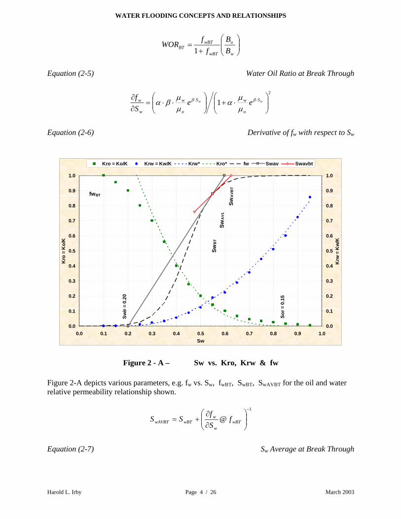
Figure 2 - A – Sw vs. Kro, Krw & fw Figure 2-A depicts various parameters, e.g. fw vs. Sw, fwBT, SwBT, SwAVBT for the oil and water relative permeability relationship shown.
1
@−
⎟⎟⎠
⎞⎜⎜⎝
⎛∂∂
+= wBTw
wwBTwAVBT f
Sf
SS
Equation (2-7) Sw Average at Break Through
Harold L. Irby Page 4 / 26 March 2003

WATER FLOODING CONCEPTS AND RELATIONSHIPS
( ) oipwiwAVBTpBT BVSSN ⋅−= Equation (2-8) Cumulative Oil Production at Break Through Volume injected at break through:
( ) pwiwAVBTiBT VSSV ⋅−= Equation (2-9) Cumulative Volume Injected at Break Through The estimated time to break through is:
iiBTBT QVT = Equation (2-10) Estimated Time to Break Through
⎥⎦
⎤⎢⎣
⎡−−−
=orwi
wiwAVBTrBT SS
SSE
1 ( % of Vd, Displaceable Volume )
Equation (2-11) Recovery Factor at Break Through, % of Vd
wiwAVBTrBT SSE −= ( % of Vp, Pore Volume ) Equation (2-12) Recovery Factor at Break Through, % of Vp It is advantageous to have an estimate of oil production, recovery factor etc. as a function of time for economic considerations and/or modeling for incremental economics with respect to implementing a given water flood project. Np as a function of average water saturation:
( ) oiwiwAVpp BSSVN −⋅= Equation (2-13) Cumulative Oil Production, Np, Oil production rate as a function of fraction water flow:
( ) oiwio BfQQ −⋅= 1 Equation (2-14) Oil Production Rate, Qo Time function can be estimated as:
ii QVT = Equation (2-15) Time Scale
Harold L. Irby Page 5 / 26 March 2003

WATER FLOODING CONCEPTS AND RELATIONSHIPS
The total recovery factor then can be determined from:
NNE pr = ( % of OOIP ) Equation (2-16) Recovery Factor, Np/N
1
10
100
1,000
10,000
0.0 1.0 2.0 3.0 4.0 5.0 6.0 7.0 8.0
t (Yrs)
0.00
0.10
0.20
0.30
0.40
0.50
0.60
0.70
0.80
Qo (Bbls/d) Qo (Bbls/d) 0.612 B-L RF (%Vd) 0.720 B-L RF (%Vd) WOR_Pi WOR_Pb
Qi (Bbls/d) = 500 f/ Pi
Qi (Bbls/d) = 555 f/ Pb
Figure 2 - B – WOR, Qo, Qi, B-L RF vs. Time (Yrs.)
Figure 2-B shows the results of applying the Buckely-Leverett Approach to the data previously shown in Figure 2-A with differing injection rates one starting from the initial reservoir pressure and the other start at bubble point pressure. The rapidly increasing WOR and diminishing oil flow rates are clearly identifiable. Note that the recovery efficiency is linear with respect to time using this approach.
Harold L. Irby Page 6 / 26 March 2003

WATER FLOODING CONCEPTS AND RELATIONSHIPS
Material Balance Approach
Using the material balance approach assumes that the flow with the reservoir is incompressible and that the reservoir volume is constant and the fluids entering the reservoirs volume are via injection and production wells. Start of the water flood is at x where x designates the corresponding values at that point in time and/or pressure. A tank model is assumed.
III. Water Flooding Above Bubble Point Pressure The water flood is start at a pressure between initial and bubble point:
oxoxpx BSVNN ⋅−= Equation (3-0) Cumulative Oil Production @ Start of Water Flood Applying the assumption/approximation of Sox = Soi we can derive the primary recovery efficiency at the start of the water flood:
( )oxoirp BBE −= 1 Equation (3-1) Primary Recovery Efficiency @ Start of Water Flood
( ) oioroiD SSSE −= Equation (3-2) Maximum Displacement Efficiency
diV VWE = Equation (3-3) Sweep Efficiency
( ) ( )DVoior EEBBE ⋅−⋅−= 11 Equation (3-4) Total Recovery Efficiency
( ) ( )Doioxmxr EBBE −⋅−= 11_ Equation (3-5) Maximum Total Recovery Efficiency
( )[ ]oioivoorvpp BSEBSEVNN ⋅−+⋅⋅−= 1
Equation (3-6) Cumulative Oil Produced
Harold L. Irby Page 7 / 26 March 2003

WATER FLOODING CONCEPTS AND RELATIONSHIPS
With appropriate substitutions and assumptions Np becomes:
( )[ ]vDooipp EEBSVNN ⋅−+⋅−= 1
Equation (3-7) Cumulative Oil Produced
E_R_Prx
E_R_mx
E_R_Pb
0.0
0.1
0.2
0.3
0.4
0.5
0.6
0.7
0.8
0.9
1.0
0.0 0.1 0.2 0.3 0.4 0.5 0.6 0.7 0.8 0.9 1.0E_V
E_R
E_R Thrtcl E_R (>Pb)
Figure 3 - A – Ev vs. Er – Water Flood Above Bubble Point Pressure Figure 3-A shows the theoretical and the computed values for Er and Ev for the data used in this document.
Harold L. Irby Page 8 / 26 March 2003

WATER FLOODING CONCEPTS AND RELATIONSHIPS
IV. Water Flooding Below Bubble Point Pressure The water flood is started below the bubble point pressure. Gas saturation of a function of Oil Formation Volume Factor, Box, where x designates the corresponding values at the point in time and/or pressure below bubble point pressure at which water flood is started and the Primary Recovery, Erp, a function of Box, Npx and Sox is as follows:
⎟⎟⎠
⎞⎜⎜⎝
⎛⋅−=
oi
ox
ox
oirp S
SBB
E 1
Equation (4-0) Total Primary Recovery Efficiency
( )⎥⎦
⎤⎢⎣
⎡−⋅−⋅= rp
oi
oxoigx E
BB
SS 11
Equation (4-1) Gas Saturation Function of Primary Recovery
⎟⎟⎠
⎞⎜⎜⎝
⎛⋅−=
ox
oxppx B
SVNN
Equation (4-2) Oil Produced From Primary Recovery At the end of the fill up period Np and Ev are estimated as follows:
( )⎥⎦
⎤⎢⎣
⎡−⋅−⋅= fur
oi
oxoifug E
BB
SS @@ 11
Equation (4-3) Gas Saturation at End of Fill Up
( )( )oroifugfuV SSSE −= @@ Equation (4-4) Sweep Efficiency at End of Fill Up
( ) ( )( ) oxoirppoxorrppfup BSEVBSEVN ⋅−⋅+⋅⋅= 1@ Equation (4-5) Oil Produced at End of Fill Up
NNE fupfur @@ = Equation (4-6) Total Recovery Efficiency at End of Fill Up
Harold L. Irby Page 9 / 26 March 2003

WATER FLOODING CONCEPTS AND RELATIONSHIPS
During the water flooding after fill up:
( ) oioroiD SSSE −= Equation (4-7) Maximum Displacement Efficiency
( ) dwpiV VBWWE ⋅−= Equation (4-8) Sweep Efficiency
( ) ( )DVooir EEBBE ⋅−⋅−= 11 2 Equation (4-9) Total Recovery Efficiency
( ) ( )( ) ooiVpoorVpp BSEVBSEVNN ⋅−⋅+⋅⋅−= 1 Equation (4-10) Oil Produced During Water Flood
MAX
End
FU
Sta
rt FU
Prmry0.0
0.1
0.2
0.3
0.4
0.5
0.6
0.7
0.8
0.9
1.0
0.0 0.2 0.4 0.6 0.8 1.0E_V
E_R
Thrtcl E_R_(<Pb) E_R#(<Pb) Piston-Like
Figure 4 - A – Ev vs. Er – Water Flood Below Bubble Point Pressure
2 Note that Er is essentially a function of Bo and a Material Balance computation can be used to create Bo as a
function of time and/or pressure.
Harold L. Irby Page 10 / 26 March 2003

WATER FLOODING CONCEPTS AND RELATIONSHIPS
V. Gas Reservoirs The recovery for a depleted volumetric gas reservoir, Ep, is:
ga
girp B
BE −= 1
Equation (5-1) Recovery Factor Depleted Gas Reservoir where Bgi and Bga are gas formation volume factors in ft^3/scf. Should the depleted gas reservoir be water flooded, then the ultimate recovery, Ewf, can be expressed as:
giga
grgiwf SB
SBE
⋅
⋅−= 1
Equation (5-2) Ultimate Recovery Factor Depleted Gas Reservoir Where Sgi is the initial gas saturation and Sgr is the residual gas saturations. Incremental gas recovery resulting from the water flood is:
⎟⎟⎠
⎞⎜⎜⎝
⎛−=−=∆
gi
gr
ga
gipwf S
SBB
EEE 1
Equation (5-3) Incremental Gas Recovery
Harold L. Irby Page 11 / 26 March 2003

WATER FLOODING CONCEPTS AND RELATIONSHIPS
VI. Recovery Efficiency Comparsions 3 The following figure compares the total recovery efficiencies from Material Balance with out water flooding, the Buckley-Leverett approach, Material Balance with water flooding started above the bubble point pressure and via Material Balance with water flooding started below the bubble point pressure.
0%
10%
20%
30%
40%
50%
60%
70%
80%
90%
100%
0.0 1.0 2.0 3.0 4.0 5.0 6.0 7.0
Time(Yr)
0.00
0.05
0.10
0.15
0.20
0.25
0.30
0.35
0.40
0.45
0.50
Sg(v/v) Sgx_wf Np/N(v/v) B-L RF (Np/N) E_R#(<Pb) E_R (>Pb)
Qi (Bbls/d) = 500 f/ Pi
Figure 5 - A – Recovery Efficiency Comparison – Via Models Note that the recovery efficiencies (except for the Np/N derived from the Material Balance computations) are linear in later time and hence will yield recovery efficiencies greater than 1 which would not be exactly correct.
3 Np/N is Primary Recovery from the Material Balance computations;
Qi, Injection Rate is 500 (bbl/d) B-L is Buckley Leverett Approach (<Pb) is Material Balance Approach Below Bubble Point Pressure and (>Pb) is Material Balance Approach Above Bubble Point Pressure
Harold L. Irby Page 12 / 26 March 2003

WATER FLOODING CONCEPTS AND RELATIONSHIPS
The author has adopted a modified asymptotic approach where the modeled water flood recovery efficiencies are adjusted with respect to the maximum displacement efficiency. In this regard, actual production data can be better matched for future production/injection projections.
0%
10%
20%
30%
40%
50%
60%
70%
80%
90%
100%
0.0 1.0 2.0 3.0 4.0 5.0 6.0 7.0
Time(Yr)
0.00
0.05
0.10
0.15
0.20
0.25
0.30
0.35
0.40
0.45
0.50
Sg(v/v) Sgx_wf Np/N(v/v) B-L RF (Np/N) E_R#(<Pb) E_R (>Pb)
Qi (Bbls/d) = 500 f/ Pi
Figure 5 - B – Recovery Efficiency Comparison - Modified 4
4 Np/N is Primary Recovery from the Material Balance computations;
Qi, Injection Rate is 500 (bbl/d) B-L is Buckley Leverett Approach Modified Via ED Asymptote (<Pb) is Material Balance Approach Below Bubble Point Pressure Modified Via ED Asymptote and (>Pb) is Material Balance Approach Above Bubble Point Pressure Modified Via ED Asymptote
Harold L. Irby Page 13 / 26 March 2003

WATER FLOODING CONCEPTS AND RELATIONSHIPS
100
1,000
10,000
0.0 1.0 2.0 3.0 4.0 5.0 6.0 7.0
Time(Yr)
10
100
1,000
Np(Mbbl) Np_WF(<Pb) Np_WF(>Pb) Qo(bbl/d) Qo_WF(<Pb) Qo_WF(>Pb)
Figure 5 - C – Production Profile Comparison – Via Models
100
1,000
10,000
0.0 1.0 2.0 3.0 4.0 5.0 6.0 7.0
Time(Yr)
10
100
1,000
Np(Mbbl) Np_WF(>Pb)' Np_WF(<Pb) Qo(bbl/d) Qo_WF(>Pb) Qo_WF(<Pb)
Figure 5 - D – Production Profile Comparison - Modified
Harold L. Irby Page 14 / 26 March 2003

WATER FLOODING CONCEPTS AND RELATIONSHIPS
VII. Dykstra-Parsons’ Method The reservoir is characterized by stratified non-uniform layers a varying permeability. In this reservoir the injected water will advance more rapidly in the higher permeability layers. The volumetric sweep efficiency, EV, then becomes a measure of the three-dimensional effect of the reservoir layering, the invasion sweep efficiency, Ei, and the macroscopic sweep efficiency, Es.
siV EEE ⋅= Equation (7-1) Volumetric Sweep Efficiency The Dykstra-Parson’s Method is used to approximate the water flood performance for stratified non-uniform layered reservoirs. The Dykstra-Parsons’ Method incorporates the following assumptions in order to make the associated computations practical:
1. The reservoir layers are of equal thickness with each layer having uniform horizontal and vertical perm abilities and that no cross flow exists between layers.
2. Piston like displacement occurs such that only one fluid phase is flowing in any given volume within the reservoir layer.
3. Steady state flow in a linear direction occurs. 4. The flowing and in-situ fluids are immiscible and incompressible. 5. The pressure profile within each layer is the same. 6. Fill-up occurs in each layer prior to incremental production as a result of water flooding.
Fill-up times should be considered with respect to the total water flooding application. 7. Each reservoir layer has the same rock and fluid properties with only the layer’s absolute
permeability differentiating them.
K1 ∆h1 I W A T E R P ∆C1=K1∆h1
K2 ∆h2 N R ∆C2=K2∆h2
K3 ∆h3 J O ∆C3=K3∆h3
E D
C U
Kj ∆hj T C ∆Cj=Kj∆hj Cj=Σ∆Cj
Kj+1 ∆hj+1 O E ∆Cj+1=Kj+1∆hj+1
R R
Kn ∆hn O I L ∆Cn=Kn∆hn Cn=Σ∆Cn
Figure 7 - A – Displacement of Oil by Water in a Stratified Reservoir
Harold L. Irby Page 15 / 26 March 2003

WATER FLOODING CONCEPTS AND RELATIONSHIPS
∆C is incremental capacity ( k⋅h (md-ft) ) and C is cumulative capacity and h is reservoir interval height (ft). The oil and water invasion profiles for the system are diagrammed in Figure 7-A. For the ith layer where the flood front is located at xi and ∆Pi is the pressure differential between the front and the producing point of the ith layer are:
iwiw x
PkAQ ∆⋅⋅= λ
Equation (7-2) D-P ith Layer Water Flow Rate
i
ioio xL
PPkAQ
−∆−∆
⋅⋅⋅= λ
Equation (7-3) D-P ith Layer Oil Flow Rate Where ∆P is the pressure differential between the efflux end of the layer and the influx end at a distance L apart. Therefore the pressure differential can be expressed as:
( )oi
io
wi
iw
kAxLQ
kAxQ
Pλλ ⋅⋅−⋅
+⋅⋅⋅
=∆
Equation (7-4) Pressure Differential ith Layer Assuming that the jth layer has been broken through by the water flood then all layers with permeability greater than that of the jth layer will also have been broken through. Therefore the fraction of the reservoir for which the layers have been completely flooded out is (j/n). Those layers having permeability less than the jth layer will only be partially swept. The (fractional) total recovery efficiency, Ei, which is defined as the fraction of the reservoir which has been invaded by water can be derived and the relationship is as follows: 5 {The reader is referred to the various references for the derivations which will not be presented here.}
( )⎥⎥
⎦
⎤
⎢⎢
⎣
⎡
⎟⎟⎠
⎞⎜⎜⎝
⎛−+⋅
−−
−⋅−
+= ∑>=
n
jii j
ii M
kk
MMM
Mjnjn
E5.0
22 11
11
)(1
Equation (7-5) Fractional Total Recovery Efficiency ith Layer When the jth layer has broken through, only water is flowing in the layers with permeability greater than that of the jth layer. Hence, the water flow rate is: 5 Dykstra, H., and Parsons, R.L., “The Prediction of Oil Recovery by Waterflood”, Chapter 12, Secondary
Recovery of Oil in the United States, 2nd Edition, API, New York, NY, 1950.
Harold L. Irby Page 16 / 26 March 2003

WATER FLOODING CONCEPTS AND RELATIONSHIPS
∑<=
⎥⎦
⎤⎢⎣
⎡ ∆⋅⋅
⋅=
n
jii w
rwiw L
PAkkQ
µ
Equation (7-6) D-P Water Flow Rate Only oil is flowing within the layers with permeability less than that in the jth layer:
( )∑>=
⎪⎪⎪
⎭
⎪⎪⎪
⎬
⎫
⎪⎪⎪
⎩
⎪⎪⎪
⎨
⎧
⎥⎥⎦
⎤
⎢⎢⎣
⎡−⋅+
∆⋅⋅⋅
=n
jii
j
i
w
rwi
o
Mkk
M
LPk
kAQ 5.0
22 1
µ
Equation (7-7) D-P Oil Flow Rate And the water oil ratio, WOR = Qw/Qo, when the jth layer has broken through is:
( )∑
∑
>=
−=
⎥⎥⎦
⎤
⎢⎢⎣
⎡−⋅+
=n
jii j
ii
n
jiii
Mkk
Mk
kWOR 5.0
22 1
Equation (7-8) Volumetric Sweep Efficiency
Harold L. Irby Page 17 / 26 March 2003

WATER FLOODING CONCEPTS AND RELATIONSHIPS
VIII. Modified Dykstra-Parsons’ Method The “Permeability Variation”, Vk, is defined as the median permeability minus the permeability at 84.1 cumulative percent divided by the median permeability, k50. In the Modified Dykstra-Parsons’ Method, only the Permeability Variation is necessary to characterize the distribution in so far has the computations are concerned since it is the magnitudes of the permeability are not so important in as much as only the ratios of permeability that occur in the calculations.
50
1.8450
kkk
Vk−
=
Equation (8-1) D-P Permeability Variation Vertical Sweep Efficiency is also known as and/or referred to as Coverage. Dykstra and Parsons constructed Coverage versus Permeability Variation which gives WOR as a function of Vk and Mobility, M. Hence for any coverage computation a set of curves at WOR’s of 0.1, 0.2, 0.5, 1, 2, 5, 10, 25, 50 and 100 are needed. Fassihi et. al. improved the coverage curves of Dykstra and Parsons with empirical correlations and are shown in Appendix Two. The Y correlation parameter was correlated in the form:
( ) ( )( ) ( )kVf
k
k
VM
VWORY
108094.0137.1
499.2948.184.0
⋅⋅−+
⋅−⋅+= 6
Equation (8-2) Y-Correlation Parameter
( ) 26453.19735.06891.0 kkk VVVf ⋅+⋅+−= Equation (8-3) Y-Correlation Exponent Function The Y-Correlation factor and Vertical Sweep Efficiency can also be expressed as:
( ) 32 11aa CCaY −⋅⋅=
Equation (8-4) Y-Correlation and Coverage
Table 1 – Y-Correlation and Coverage Constants a1 3.3340888568
a2 0.7737348199
a3 -1.225859406
6 Fassihi, M. R., New Correlations for Calculation of Vertical Coverage and Areal Sweep Efficiency, SPE
Reservoir Engineering, November 1986.
Harold L. Irby Page 18 / 26 March 2003

WATER FLOODING CONCEPTS AND RELATIONSHIPS
Areal Sweep Efficiency, EA, is the fraction of the water flood pattern area actually contacted by water. EA is a function of the pattern geometry, the mobility ratio, M, and the volume of water injected, Wp. Fassihi et. al. correlated daya from Dyes et. al. for a correlation for EA:with correlation constants listed in Table 3.
( )[ ] ( ) 654321 lnln1 aaMafaaMaE
Ew
A
A ++⋅+⋅++⋅=−
Equation (8-5) Areal Sweep Efficiency Correlation
Table 2 – Coefficients in Areal Sweep Efficiency Correlations 7
Coefficient 5-Spot Direct Line Staggered Line
a1 -0.2062 -0.3014 -0.2077
a2 -0.0712 -0.1568 -0.1059
a3 -0.5110 -0.9402 -0.3526
a4 0.3048 0.3714 0.2608
a5 0.1230 -0.0865 0.2444
a6 0.4349 -0.8805 0.3158
And the Volumetric Sweep Efficiency is:
( ) ( )[ ]{ }25.05.0 11 DA
DAV
EEMM
EEE
−⋅−−=
Equation (8-6) Volumetric Sweep Efficiency
7 Ibib.
Harold L. Irby Page 19 / 26 March 2003

WATER FLOODING CONCEPTS AND RELATIONSHIPS
APPENDIX ONE
Nomenclature Symbol Definition Units A Reservoir or Contour Area acres Bo Oil Formation Volume Factor rb/bbl Boi Initial Oil Formation Volume Factor rb/bbl EA Areal Sweep Efficiency v/v ED Displacement Efficiency (Microscopic) v/v Ei Invasion Sweep Efficiency v/v Er Total Recovery Efficiency v/v Erp Total Primary Recovery Factor v/v EV Sweep Efficiency (Macroscopic) v/v
fw Fractional Flow v/v h Reservoir or Contour Height ft ko Oil Permeability md kro Relative Oil Permeability v/v krw Relative Water Permeability v/v kw Water Permeability md λo Oil Mobility darcy/cp λw Water Mobility darcy/cp M Mobility Ratio (M_Displacing/M_Displaced) µo Oil Viscosity cp MOS Movable Oil Saturation v/v µw Water Viscosity cp N OOIP rbbl
Np Oil Produced (at time and/or pressure) bbl Qi Water or Fluid Injection Rate bbl/d
Sg Gas Saturation v/v Soi Initial Oil Saturation v/v Sor Residual Oil Saturation v/v SwAV Average Water Saturation v/v Swi Initial Water Saturation v/v Swir Irreducible Water Saturation v/v T Time days or yrs TBT Time to Water Break Through days or yrs Vd Displaceable Volume rbbl
Harold L. Irby Page 20 / 26 March 2003

WATER FLOODING CONCEPTS AND RELATIONSHIPS
Vi Volume of Injected Water or Fluid bbl Vk Permeability Variation v/v Vp Pore Volume rbbl
WOR Water Oil Ratio v/v
Harold L. Irby Page 21 / 26 March 2003

WATER FLOODING CONCEPTS AND RELATIONSHIPS
APPENDIX TWO
Vertical Coverage and Areal Sweep Efficiency
Figure A-2-1 – The Actual and The Correlated Areal Sweep Efficiencies 8
8 Fassihi, M. R., O’Brien, W. J., A Predictive Model for Water Flood Performance Using a Handheld Calculator, ARCO Oil and Gas Co., Plano, Texas, July 1984.
Harold L. Irby Page 22 / 26 March 2003

WATER FLOODING CONCEPTS AND RELATIONSHIPS
Figure A-2-2 – Coverage as a Function of Permeability Variation and Mobility Ratio 9
9 Fassihi, M. R., O’Brien, W. J., A Predictive Model for Water Flood Performance Using a Handheld Calculator, ARCO Oil and Gas Co., Plano, Texas, July 1984.
Harold L. Irby Page 23 / 26 March 2003
WATER FLOODING CONCEPTS AND RELATIONSHIPS
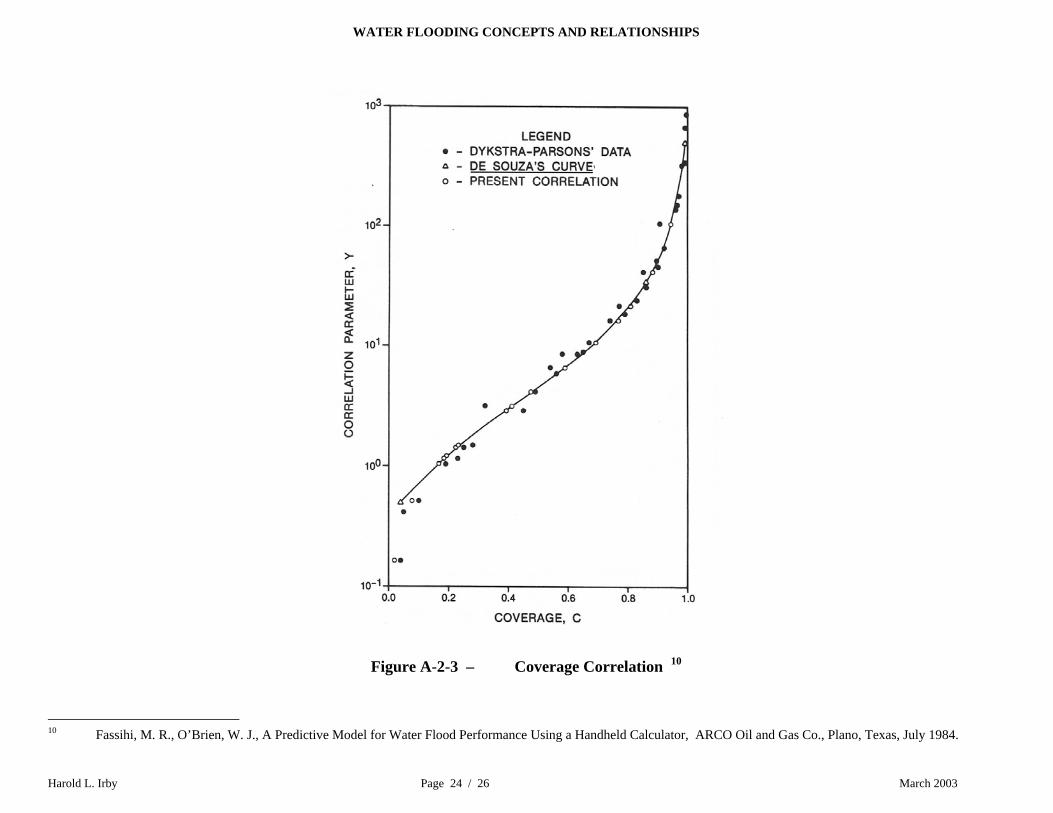
Figure A-2-3 – Coverage Correlation 10
10 Fassihi, M. R., O’Brien, W. J., A Predictive Model for Water Flood Performance Using a Handheld Calculator, ARCO Oil and Gas Co., Plano, Texas, July 1984.
Harold L. Irby Page 24 / 26 March 2003

WATER FLOODING CONCEPTS AND RELATIONSHIPS
REFERENCES 1. Bassiouni, Zaki, IHRDC Waterflooding, Saudi Aramco, September 2-6, 2000, Dhahran, Saudi Arabia.
2. Dykstra, H., and Parsons, R.L.: “The Prediction of Oil Recovery by Waterflood,” Chapter 12, Secondary Recovery of Oil in the United States, 2nd Edition, API, New York, NY, 1950.
3. Fassihi, M. R., O’Biren, W. J., A Predictive Model For Waterflood Performance Using A Hand Held Calculators, ARCO Oil and Gas Company, Plano, Texas, July 1984.
4. Craig, Forrest F. Jr., The Reservoir Engineering Aspects of Waterflooding, SPE Monograph Volume 3, 1971.
5. Fassihi, M.R., New Correlations for Calculation of Vertical Coverage and Areal Sweep Efficiency, SPE Reservoir Engineering, November 1986.
6. Slider, H. C., “Worldwide Practical Petroleum Reservoir Engineering Methods,”, Chapter 9.Water Flooding and its Variations, Pennwell Books, Tulsa, Oklahoma, 1983.
7. Willhite, Paul G. Waterflooding - SPE Textbook Series Vol. 3, 7th Printing 2001, Society of Petroleum Engineers, Richardson, TX 1986.
Harold L. Irby Page 25 / 26 March 2003

WATER FLOODING CONCEPTS AND RELATIONSHIPS
INDEX
Bassiouni, iii Buckley-Leverett, 3
Dykstra-Parson’s, 15 Fassihi, 18
Harold L. Irby Page 26 / 26 March 2003
Recommended


![Linear Displacement Effficiency_In waterflooding [Compatibility Mode]](https://img.dokumen.tips/doc/110x75/551c750b49795911568b4724/linear-displacement-effficiencyin-waterflooding-compatibility-mode.jpg)