ORIGINAL PAPER
Urban heat islands in Hong Kong: statistical modelingand trend detection
Weiwen Wang1 • Wen Zhou2 • Edward Yan Yung Ng1,3,4 •
Yong Xu3
Received: 11 November 2015 / Accepted: 6 May 2016� Springer Science+Business Media Dordrecht 2016
Abstract Urban heat islands (UHIs), usually defined as temperature differences between
urban areas and their surrounding rural areas, are one of the most significant anthropogenic
modifications to the Earth’s climate. This study applies the extreme value theory to model
and detect trends in extreme UHI events in Hong Kong, which have rarely been docu-
mented. Extreme UHI events are defined as UHIs with intensity higher than a specific
threshold, 4.8 for summer and 7.8 �C for winter. Statistical modeling based on extreme
value theory is found to permit realistic modeling of these extreme events. Trends of
extreme UHI intensity, frequency, and duration are introduced through changes in
parameters of generalized Pareto, Poisson, and geometric distributions, respectively.
During the 27-year study period, none of the quantities in winter analyzed in this study
increased significantly. The annual mean summertime daily maximum UHI intensities,
which are samples from a Gaussian distribution, show an increasing but nonsignificant
linear trend. However, the intensity of extreme UHI events in summer is increasing sig-
nificantly, which implies that the risk of mortality and heat-related diseases due to heat
stress at night (when the daily maximum UHI occurs) in summer is also increasing. The
warming climate has threatened and will continue to threaten inhabitants of this subtropical
high-density city. Strategies for adaptation to and mitigation of climate change, such as
adding greenery and planning a city with good natural ventilation, are needed.
& Wen [email protected]
1 School of Architecture, The Chinese University of Hong Kong, Hong Kong SAR, China
2 Guy Carpenter Asia-Pacific Climate Impact Centre, School of Energy and Environment, CityUniversity of Hong Kong, Hong Kong SAR, China
3 Institute of Future Cities, The Chinese University of Hong Kong, Hong Kong SAR, China
4 Institute of Environment, Energy and Sustainability, The Chinese University of Hong Kong,Hong Kong SAR, China
123
Nat HazardsDOI 10.1007/s11069-016-2353-6
Author's personal copy

Keywords Urban heat island � Extreme value theory � Peaks-over-threshold model �Generalized Pareto distribution � Parametric trend
1 Introduction
Urban heat islands (UHIs) are urban areas that tend to have higher temperatures than
surrounding rural areas, and they are one of the most significant anthropogenic modifi-
cations to the Earth’s climate (Oke 1982; Zhao et al. 2014; Zhou et al. 2015). With the
ever-increasing urban population, more and more people are vulnerable to problems caused
by urbanization (Memon et al. 2008). According to the World Health Organization, the
urban population in 2014 accounted for 54 % of the total global population, up from 34 %
in 1960, and continues to grow. Meanwhile, the Intergovernmental Panel on Climate
Change (IPCC) has reported that climate warming is unequivocal, and the frequency of
heat waves has increased in large parts of Europe, Asia, and Australia (IPCC 2013). Urban
areas are especially vulnerable to heat waves due to the existence of UHIs and synergistic
interactions between UHIs and heat waves (Li and Bou-Zeid 2013; Li et al. 2015).
Hong Kong is a high-density city in the subtropics with a hot and humid climate. The
UHI effect in Hong Kong has been investigated extensively. Some studies _ENRE-
F_6_ENREF_6 have characterized the spatial pattern of the UHI in Hong Kong using land
surface temperatures retrieved from remote sensing data (Fung et al. 2009; Liu and Zhang
2011), and others have evaluated the reliability of UHI intensity as an indicator of urban
heating (Memon et al. 2009). Strategies of urban planning for adaptation to and mitigation
of UHIs are of interest to the government and researchers in Hong Kong as well (Girid-
haran et al. 2007; Ng 2009; Ng et al. 2012). But studies of UHIs under the background of
secular climate change in Hong Kong have not yet been undertaken, possibly in part
because of the lack of long-term observations in rural areas.
In previous studies of hazards related to urbanization, long-term trends in meteoro-
logical disasters such as heat waves, rainstorms, and haze have been addressed (Chan and
Zhou 2005; Shi and Cui 2011; Yan et al. 2011; Wei et al. 2011; Habeeb et al. 2015; Liu
et al. 2014, 2015; Qian 2015; Xia et al. 2015). Changes in heat-related mortality in
metropolitan areas have been detected as well (Hondula and Davis 2014; Kim et al. 2015;
Sheridan et al. 2008). However, as an environmental hazard, UHIs have rarely been
directly investigated in terms of their extremes. The objective of this study is to define
extreme UHI events, model their behavior, and detect their temporal trends in Hong Kong
based on extreme value theory.
There is a long tradition of using extreme value theory in meteorological and envi-
ronmental applications. In the modern theory, the peaks-over-threshold model is used to
describe all exceedances above a high threshold rather than just looking at the block
maxima (e.g., the annual maximum daily precipitation amount). The theory has been
extended to encompass temporal trends. The most common approach for dealing with
nonstationarity is to allow for parametric changes with time in the distribution (Garcia-
Aristizabal et al. 2014; Smith 1989). The approach jointly models the occurrence of an
event (an exceedance of a high threshold) and its severity (the magnitude of the excess over
a high threshold). The exceedances are assumed to occur according to a Poisson distri-
bution, while the excesses above the threshold are assumed to follow a generalized Pareto
(GP) distribution (Coles 2001). More recently, approaches to modeling the duration of
Nat Hazards
123
Author's personal copy
extreme events such as heat waves and cold waves, rather than discarding these clusters,
have been advocated (Furrer et al. 2010; Parey and Hoang 2015). Based on the most recent
developments in extreme value analysis, an appropriate peaks-over-threshold model of
extreme UHI events in Hong Kong for both summer and winter will be set up in this paper.
2 Data and methodology
2.1 Observations and definition of UHIs in Hong Kong
The Hong Kong Observatory Headquarters (HKO) is a representative urban weather sta-
tion and a common choice of UHI studies in Hong Kong (Fung et al. 2009; Memon et al.
2009). In this study, we chose HKO as the urban site and three other weather stations, Ta
Kwu Ling (TKL), Tsak Yue Wu (TYW), and Waglan Island (WGL), as rural sites to
quantify UHI intensities in Hong Kong. The locations of these weather stations are shown
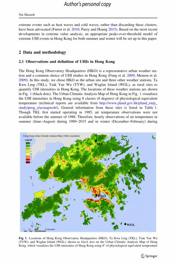
in Fig. 1 (black dots). The Urban Climatic Analysis Map of Hong Kong in Fig. 1 visualizes
the UHI intensities in Hong Kong using 8 classes (8 degrees) of physiological equivalent
temperature (technical reports are available from http://www.pland.gov.hk/pland_en/p_
study/prog_s/ucmapweb/). General information from these sites is listed in Table 1.
Though TKL first started operating in 1985, air temperature observations were not
available before the summer of 1988. Therefore, hourly observations of air temperature in
summer (June–August) during 1989–2015 and in winter (December–February) during
Fig. 1 Locations of Hong Kong Observatory Headquarters (HKO), Ta Kwu Ling (TKL), Tsak Yue Wu(TYW), and Waglan Island (WGL), shown as black dots on the Urban Climatic Analysis Map of HongKong, which visualizes the UHI intensities of Hong Kong using 8� of physiological equivalent temperature
Nat Hazards
123
Author's personal copy

1988/1989–2014/2015 from HKO and TKL are used in this study. Hourly temperature
records from WGL are available and utilized 1 year later and from TYW 7 years later
(summer during 1996–2015 and winter during 1995/1996–2014/2015). A UHI is defined as
the temperature difference between HKO and a rural counterpart, while extreme UHI
events are defined as UHIs with intensities higher than a specific high threshold. In
addition, hourly relative humidity and daily maximum temperature records from HKO as
well as daily rainfall records from both HKO and TKL are further used to elucidate
possible causes of changes and impacts of extreme UHIs in Hong Kong.
2.2 Satellite images for land cover changes
Located on the southeast coast of China, facing the South China Sea, Hong Kong is
affected by clouds most of the time, from early January to late September. To show the
land cover change in Hong Kong and adjacent Shenzhen, we collected 8 clear Landsat
images for 2 time periods, including 4 Landsat images from the year 1994 (October 1,
October 24, October 24, and November 2) and 4 images from the years 2013–2015 (Oc-
tober 5, 2013, December 31, 2013, August 8, 2015, and October 18, 2015). All Landsat
data can be downloaded from the US Geological Survey Web site: http://glovis.usgs.gov.
Herein, all Landsat images are atmospherically corrected into surface reflectance using the
Landsat Ecosystem Disturbance Adaptive Processing System (Masek et al. 2006). After
this atmospheric correction, two sets of Landsat data from two periods are geometrically
corrected and seamlessly joined into two large images to cover Hong Kong and nearby
regions of Shenzhen.
2.3 Atmospheric reanalysis and anomaly composite
Reanalysis data during 2005–2014, including the daily mean air temperature at 2 m, mean
sea level pressure, and geopotential height, are taken from the National Centers for
Environmental Prediction-National Center for Atmospheric Research (NCEP-NCAR)
reanalysis (Kalnay et al. 1996). Daily anomalies derived from a smoothed mean daily
annual cycle are used to examine the atmospheric characteristics associated with extreme
UHIs. These daily anomalies are averaged in corresponding extreme UHI days, and the
Student’s t test is used to test their significance.
Table 1 General information from meteorological stations for Hong Kong UHI analysis in this study
Information Hong Kong ObservatoryHeadquarters
Ta KwuLing
Tsak YueWu
WaglanIsland
Abbreviated name HKO TKL TYW WGL
WMO code 45005 45032 – 45045
Longitude (E) 114�1002700 114�0902400 114�1902400 114�1801200
Latitude (N) 22�1800700 22�3104300 22�2401100 22�1005600
Elevation above mean sealevel (m)
32 15 5 56
Date of first operation 2 Mar 1883 14 Oct1985
1 Oct 1995 1 Dec 1952
Nat Hazards
123
Author's personal copy

2.4 Extreme value theory
In the present study, the peaks-over-threshold method is utilized to model the intensity,
frequency, and duration of extreme UHI events. Specifically, the intensity above the
threshold of UHI is modeled by a GP distribution, the annual frequency is modeled by a
Poisson distribution, and the duration is modeled by a geometric distribution (Furrer et al.
2010). A GP distribution is given by
F x; n; ru; uð Þ ¼ 1� 1þ nx� u
ru
� ��1n
; x[ u; 1þ nx� u
ru[ 0 ð1Þ
where n stands for the shape parameter, and ru[ 0 denotes the scale parameter depending
on the selected threshold u.
The Poisson distribution is given by
PðkÞ ¼ kke�k
k!; k ¼ 0; 1; 2; . . . ð2Þ
where k is the number of events in a given year. A geometric distribution that can model
the length (duration) of an extreme event is given by
PðkÞ ¼ 1� hð Þk�1h; k ¼ 1; 2; . . . ð3Þ
with the reciprocal of the parameter h being the mean.
The extreme value analysis is based on the assumption that extreme events occur
independently. However, extreme events can occur in succession in the case of persistent
weather conditions. After the threshold is calibrated in this study, the geometric distri-
bution is applied to check the probability of continuity. If the continuous probability of
extreme UHIs is high, the use of geometric distribution can cluster extreme UHI days
occurring successively into a single extreme event. Otherwise, the duration cluster can be
discarded, and a Poisson–GP model will be sufficient. The independence assumption is
therefore fulfilled.
Parameter estimation in the model is done using maximum likelihood methods. Taking
the GP distribution as an example, suppose that the values y1; y2; . . .; yk are the k excessesof a threshold u. For n 6¼ 0 the log-likelihood is derived from Eq. (1) as
l ru; nð Þ ¼ �k logru � 1þ 1
n
� �Xki¼1
log 1þ nyiru
� �: ð4Þ
Return levels can be estimated and allow better interpretation of the extreme value
model than individual parameters. Suppose that a GP distribution with parameters ru and nis a suitable model for exceedances of a threshold u by a variable X. That is, for x[ u; itfollows that
Pr X[ xf g ¼ fu 1þ nx� u
ru
� ��1n
; ð5Þ
where fu ¼ Pr X[ uf g. Hence, the level xm that is exceeded on average once every m
observations is the solution of
Nat Hazards
123
Author's personal copy

fu 1þ nxm � u
ru
� ��1n
¼ 1
m: ð6Þ
Rearranging,
xm ¼ uþ run
mfuð Þn�1h i
; ð7Þ
provided that m is sufficiently large to ensure that xm [ u. By construction, xm is the m-
observation return level.
Standard errors or confidence intervals for xm can be derived by the delta method. The
uncertainty in the estimate of fu should be included in the calculation, but life is made
simpler by ignoring the uncertainty in fu; which is usually small relative to that of other
parameters. From Eq. (7),
ru ¼xm � uð Þnmfuð Þn�1
; n 6¼ 0 ð8Þ
with fixed xm, substitution into Eq. (4) leads to a one-parameter likelihood that can be
maximized with respect to n. As a function of xm, this is the profile log-likelihood for the
m-observation return level.
The model is further extended to allow for estimating trends in extreme characteristics
of UHI intensity, frequency, and duration. One can consider parameters to be fixed within a
given year but allow shifts from 1 year to another. That is, for each year x in the record
period, ru = ru(x) for the GP scale parameter, k = k(x) for the Poisson parameter, and
h = h(x) for the geometric parameter (Wang et al. 2015c). Since changes in the shape
parameter of the GP distribution are rarely observed and difficult to model, this parameter
is kept fixed. Trends are introduced through covariate effects in the GP scale parameter,
with a generalized linear model framework in the Poisson and geometric fittings.
3 Environmental and climatic changes
Before investigating the extreme events, the environmental changes and climatological
characteristics of UHIs in Hong Kong will first be described. The Landsat images in Fig. 2
demonstrate the land cover change in Hong Kong and adjacent areas of Shenzhen from
1994 (Fig. 2a) to recent years (2013–2015, Fig. 2b). Large developments occurred in New
Territories (northern Hong Kong), where TKL is located, and in nearby Shenzhen. On the
Kowloon Peninsula, where HKO is located, a major change is that the reclaimed areas on
the east and west margins of the peninsula in Fig. 2a are mostly built up in Fig. 2b.
Vegetative cover reductions (in red) inside the peninsula are evident as well. Very limited
changes are found in Sai Kung (eastern Hong Kong), where TYW is located. This suggests
that TYW may be a better rural site than TKL. This is further demonstrated by Fig. 3,
which shows that UHI intensities are stronger when computed by records at TYW than at
TKL. However, the present study pays more attention to the long-term trend of UHI, so
TKL is a better choice because it has longer-term observations than TYW (Table 1).
According to Siu and Hart (2013), TYW was deemed the most appropriate representative
rural site in Hong Kong, but TKL can still serve as another rural reference site. WGL,
which has often been chosen as a representative rural site in early studies (Stanhill and
Nat Hazards
123
Author's personal copy

Kalma 1995; Yim and Ollier 2009), is actually not a good choice (Fig. 3), mainly because
it is a marine station (Fig. 1).
In the diurnal cycle, UHI intensities in Hong Kong are positive during the night but may
be negative during the daytime. Generally, possible causes of positive UHI intensities
Fig. 2 Landsat images of land cover over Hong Kong and adjacent Shenzhen in a 1994 and b 2013–2015.Color bar cannot be shown for these full-color maps. Roughly, red indicates vegetation, blue indicateswater, gray denotes buildings, and white denotes flat artificial covers
Nat Hazards
123
Author's personal copy

include increased absorption of solar radiation and anthropogenic heat generation,
increased thermal storage, decreased evapotranspiration, and reduced urban winds in the
urban areas (Memon et al. 2008; Oke 1987). But due to canyon shading around the urban
site, it may be cooler than the rural site during the daytime (Oke 1982). The case in Hong
Kong is more complicated. Daytime negative UHI intensity may be caused by the com-
bined effects of its coastal nature and high-rise and compact urban morphology. On the one
Fig. 3 Diurnal cycle for temperature at four weather stations of Hong Kong in a summer and b winter, anddiurnal cycle of UHI intensities calculated by three pairs of weather stations (taking HKO as the urban site)in c summer and d winter. Local standard time is used. The shadings represent one standard deviation
Fig. 4 Seasonal variation ofa normalized nocturnal (7 p.m. to7 a.m. local time) UHI intensity(solid line) in Hong Kong andrelative humidity observed atHKO (dashed line), b monthlytotal rainfall amount (mm)observed at HKO during1989–2014
Nat Hazards
123
Author's personal copy

hand, HKO is closer to the sea than TKL and TYW, which makes it cooler in the daytime.
Compared to HKO, the lower daytime temperature and phase difference in diurnal cycles
of WGL also lend support to this factor. On the other hand, a recent field model study
suggested that the cooler urban daytime phenomenon can be observed only in a high-rise
compact model, but not in a low-rise sparse model (Wang et al. 2015a).
Seasonality of UHI can be identified in Fig. 3 as well. In general, UHI intensity is
higher in winter than in summer, and the difference can be more than 2 �C. Remarkable
seasonal variation is evident in all tropical and subtropical cities reviewed by Roth (2007),
and the largest UHI intensities are usually measured during the dry season. Figure 4
indicates that this is also the case in Hong Kong: UHI intensities are highly related to
humidity and rainfall, weaker in wet seasons and stronger in dry seasons. This seasonality
of UHI can probably be explained by surface moisture differences between urban and rural
areas. As urban geometry and thermal admittance are primarily contributors of nocturnal
UHI, with little vegetative cover, urban cooling potentials do not change much throughout
Fig. 5 Annual summer mean of a daily maximum UHI intensity, daily minimum of hourly temperature atb HKO, and c TKL. Annual winter mean of d daily maximum UHI intensity, daily minimum of hourlytemperature at e HKO, and f TKL. Red (blue) dashed lines represent increasing (decreasing) trend
Nat Hazards
123
Author's personal copy

the year, while some physical properties of the rural surface, such as albedo and thermal
admittance, are subject to considerable seasonal change (Roth 2007).
The Kolmogorov–Smirnov test (Lilliefors 1967; Massey 1951) is adopted to determine
whether the UHI values are samples from a Gaussian distribution. The test shows that the
annual means of daily maximum UHI intensities (calculated separately for summer and
winter) follow a normal distribution. Therefore, we can use a least squares linear regression
to characterize the temporal trend of this quantity. For summertime, UHI intensities in
Hong Kong increase with a trend of 0.014 �C per year, but the increase is nonsignificant at
the 0.05 significance level (Fig. 5a). The next question is whether the nonsignificance of
this increasing trend is due to urban expansion, which may cause, for example, both urban
and rural areas to warm up, but the rural areas can warm even faster than the urban areas.
Because the daily maximum UHI intensities generally occur at night, particularly in the
early morning before sunrise (Fig. 3), the daily minimum of hourly temperature is used to
characterize temporal trends of temperature at both the urban and rural sites. It is found that
minimum temperature at the urban site increases nonsignificantly with a positive trend of
0.011 �C per year (Fig. 5b), while the rural site shows a slight and nonsignificant
decreasing trend (Fig. 5c). Corresponding quantities in winter are shown in Fig. 5d–f.
Minimum temperature at HKO is decreasing with a slope of -0.019 �C per year, while at
TKL it is decreasing with a larger slope of -0.026 �C per year. But the UHI intensity is
increasing with a slope of 0.009 �C per year. None of these three trends in winter is
significant at the 0.05 significance level. The above-detected trends lend support to the
choice of TKL as a representative rural site: The urban expansion in northern Hong Kong
and adjacent Shenzhen (Fig. 2) has not resulted in, at least, faster warming of TKL than
HKO.
4 Extreme values and nonlinear parametric trends
4.1 Threshold choice
As extreme value theory has not yet been applied to UHI study, the threshold has to be
chosen very carefully. We have to balance choosing a sufficiently high threshold, so that
the GP distribution of Eq. (1) is essentially satisfied, with choosing a sufficiently low
threshold, so that we have enough excesses to estimate the GP parameters. We first adopt
the criterion proposed by Coles (2001) for choosing the threshold: two graphical tools, the
mean residual life plot and the parameter stability plot. In practice, the scale parameter
needs to be adjusted to remove the dependence on the threshold. If a GP distribution is a
valid model for excesses of a threshold u0, then excesses of a higher threshold u should also
follow a GP distribution. The shape parameters of the two distributions are identical.
However, for the GP scale parameter ru for a threshold u[ u0, it follows that
ru ¼ ru0 þ n u� u0ð Þ; ð9Þ
so that the scale parameter changes with u unless n ¼ 0. This difficulty can be remedied by
adjusting the GP scale parameter as
r� ¼ ru � nu; ð10Þ
which is constant with respect to u by Eq. (9). Consequently, estimates of both r* and nshould be constant above u0, if u0 is a valid threshold for following the GP distribution.
Nat Hazards
123
Author's personal copy

Figure 6 shows the mean residual life plot and the parameter stability plot of daily
maximum UHIs fitted to the GP distribution against different threshold values in summer,
while Fig. 7 shows the plots in winter. The mean residual plots should be linear, and the
parameter estimates should be stable (constant) above the threshold at which the GP model
becomes valid. In practice, the mean excess values and parameter estimates are computed
from a relatively small quantity of data, so the plots will look only approximately linear or
constant even when the GP distribution becomes valid. Confidence intervals are included
to account for the effects of estimation uncertainty in this evaluation. In the summer case,
for instance, in the mean residual life plot (Fig. 6a), we look for approximate linearity
while keeping between the confidence bounds. Hence, a threshold above around 5.6 �C is
not appropriate because the confidence bounds increase dramatically. And it is obvious in
Fig. 6b and c that there are not enough data above a threshold of 5.6 �C. Meanwhile, by
taking a threshold below 4.4 �C, the variances in Fig. 6b and c are too small, which means
the number of observations is too large and the asymptotic approximation of Eq. (1) will be
violated. Therefore, it can be roughly estimated from Fig. 6 that the threshold for summer
extreme UHIs should be around 4.4–5.6 �C. Thresholds should be around 7.2–8.6 �C,when similar judgments are imposed on Fig. 7.
However, the two graphical tools are helpful only in seeing a range where the threshold
should occur, and this still requires a good deal of subjective judgment. Therefore, we
propose a further step for threshold selection by taking the Poisson distribution for the
frequency of extreme values into consideration. P values representing the goodness-of-fit
of the Poisson distribution in modeling extreme UHI events against different threshold
choices are given in Fig. 8. For summer, the extreme UHIs are samples from a Poisson
distribution only when the chosen threshold is not lower than 4.8 �C, and the p value is
highest when the threshold is 4.8 �C. For winter, the Poisson distribution can be satisfied
Fig. 6 a Mean residual life plot(dashed lines: confidenceintervals) and b modifiedparameter ru and c shapeparameter n estimates (errorbars: confidence intervals)against threshold values for HongKong daily maximum UHI insummer
Nat Hazards
123
Author's personal copy

with many threshold choices higher than 6.8 �C, and the p value is highest when the
threshold is 7.8 �C. Therefore, we choose 4.8 �C as the threshold of extreme UHIs for
summer and 7.8 �C for winter. These two UHI intensities are in the 97.5th percentile for
summer and the 92.5th percentile for winter.
4.2 Stationary modeling
Once the thresholds are chosen, extreme UHI events can be calculated and the stationary
peaks-over-threshold model applied. Table 2 lists the selected thresholds and fitting
Fig. 7 Same as Fig. 6 but forwinter
Fig. 8 P values represent thegoodness-of-fit of the Poissondistribution in modeling extremeUHI events against thresholdchoices for Hong Kong ina summer and b winter
Nat Hazards
123
Author's personal copy

parameters (standard errors in parentheses) of extreme UHI events in Hong Kong. The
stationary modeling results are shown in Figs. 9 and 10. The positive shape parameter in
summer and negative parameter in winter demonstrate that extreme UHIs in the two
seasons have different statistical behaviors. The fact that the longest duration of extreme
UHIs in the study period is only 3 days motivates us to discard modeling this cluster in
summer. The thresholds for defining extreme UHIs in each season are calibrated based on
extreme value theory, and we concluded that the 97.5th percentile for summer and the
92.5th percentile for winter are the best choices. To verify that the difference in the
duration of extreme UHIs between the two seasons is not simply due to a sampling
problem (i.e., discrepancy of percentile), we also calculate summer extreme UHIs using the
92.5th percentile as a threshold and model their duration with a geometric distribution
(figure not shown). It is found that the probability of 1-day duration is more than 70 %,
while the probability of 2-day duration is less than 20 %, and the probability of 3-day
duration is only 5.5 %. This is substantially lower than the case of winter in Fig. 10d,
which shows that the probability of 1-day duration is below 40 %, and the cumulative
probability of 2- to 5-day duration is up to 55 %.
A possible reason is that the weather in summer is controlled mainly by relatively short-
term atmospheric convections and conditions (Wang et al. 2014, 2016), while in winter it is
controlled by longer-term atmospheric circulations (Cheung et al. 2013, 2015; Zhou et al.
2009). To verify this possibility, we conduct composite analysis of atmospheric anomalies
corresponding to extreme UHIs in summer and winter, respectively (Fig. 11). It is obvious
that extreme UHIs in summer have a very weak relationship with large-scale anomalies,
which may imply that local, and hence short-term, atmospheric conditions are more
important in summer. Correspondingly, extreme UHIs in winter are linked with large-scale
temperature and circulation anomalies. Precipitation deficiency in the southeast coastal
regions of China is found (Fig. 11b). Associated with this dry condition, there are dipole-
like patterns in the near-surface temperature and mean sea level pressure (Fig. 11d, f):
warm episodes in the Eurasian continent but localized cold anomalies in the southern
region. Negative geopotential height anomalies are found east of eastern China at the
midlevel’s of the troposphere (Fig. 11h), corresponding to the positive mean sea level
pressure anomalies to their southwest (Fig. 11f). Abnormal sinking motions in the
southeast coastal regions are clearly seen from vertical velocity anomalies (figure not
shown), which is responsible for the regional dry condition.
Having chosen the threshold of 4.8 �C for summertime, for the period of 1989–2015
with 2484 daily maximum UHIs, we get 63 excesses. The number of extreme UHI events
accounts for about 2.5 % of the total daily observations. The scale (ru) and shape (n)
Table 2 Thresholds and fitting parameters (standard errors in parentheses) of extreme UHIs in Hong Kong
Parameters Summer Winter
Threshold (u) 4.8 �C 7.8 �CGP scale (ru) 0.74 (0.143) 1.85 (0.158)
GP shape (n) 0.03 (0.137) -0.48 (0.055)
Poisson (k) 2.33 (0.540) 2.96 (0.614)
Geometric (h) – 0.43 (0.055)
The GP, Poisson, and geometric models are used to fit intensity, frequency, and duration of extreme events,respectively
Nat Hazards
123
Author's personal copy

parameters in summer are 0.74 and 0.03, respectively. Diagnostic plots for the GP model
are generated, allowing the threshold selection to be revisited to see whether the asymp-
totic basis of the model is violated. The probability plot is not shown, as the (empirical)
circles are sufficiently close to linearity. The quantile plot and the return level plot for
summer are given in Fig. 9a and b, respectively. The circles in Fig. 9a are located close to
the unit diagonal, which lends support to the fitted GP model. There are two exceptions that
Fig. 9 a Quantile plot and b return level plot for GP distribution fitted to daily maximum UHI intensities inHong Kong summers. c Frequency of extreme UHI events in Hong Kong summers fitted to the Poissondistribution. The threshold is 4.8 �C
Fig. 10 a Quantile plot and b return level plot for GP distribution fitted to daily maximum UHI intensitiesin Hong Kong winters. c Frequency and d duration of extreme UHI events in Hong Kong winters fitted tothe Poisson and geometric distributions, respectively. The threshold is 7.8 �C
Nat Hazards
123
Author's personal copy

Fig. 11 Composite anomalies of a, b precipitation (mm); c, d near-surface temperature (�C); e, f mean sealevel pressure (Pascal); and g, h 500-hPa geopotential height (m) for extreme UHIs in Hong Kong insummers (left panels) and winters (right panels) during 2005–2014. Shading indicates regions of anomaliesthat are significant at the 0.05 level in the Student’s t test; warm (cool) colors denote positive (negative)significant anomalies. The black dot denotes the location of Hong Kong
Nat Hazards
123
Author's personal copy

are not located very close to the unit diagonal, the extreme cases in 2009 and 2013, with
UHI intensities of over 8 �C (the two circles with highest empirical UHI intensity in
Fig. 9a). However, the confidence intervals in the return level plot (Fig. 9b) suggest that
the model departures are not large after allowance for sampling. That is, nearly all of the
observed records (circles in Fig. 9b) are located between the 95 % confidence intervals
(dashed lines in Fig. 9b). Figure 9c suggests that the Poisson model can permit a realistic
modeling of extreme UHI frequency in summer. A frequency of one or two events per
summer happens most often, while the maximum occurrence can be up to seven in one
summer. A Poisson parameter (k) of 2.33 (Table 2) means the average occurrence of
extreme UHIs is 2.33 times per summer.
For wintertime, having chosen the threshold 7.8 �C for the 27 winters of
1988/1989–2014/2015, with a total of 2436 daily maximum UHIs, we get 80 extreme UHI
spells. The scale (ru) and shape (n) parameters in winter are 1.85 and -0.48, respectively.
Figure 10 suggests that the stationary peaks-over-threshold model can permit a realistic
modeling of extreme UHIs in winter. The goodness-of-fit in the quantile plot (Fig. 10a) is
convincing, and the circles are located inside the confidence intervals on the return level
plot (Fig. 10b). Figure 10c and d lends support to the fitted Poisson and geometric dis-
tributions, respectively. A Poisson parameter of 2.96 (Table 2) is also the mean frequency
of extreme UHIs in winter, while a geometric parameter of 0.43 suggests that the mean
duration of extreme UHI events is 2.32 days (the reciprocal of the geometric parameter).
4.3 Changes in extreme UHI events
It is usually more convenient to interpret the extreme value model in terms of quantiles or
return levels, rather than in terms of individual parameter values (Coles 2001). Further-
more, return levels estimated by the threshold excess model can be helpful for social
applications, such as risk assessment. This can be done by the return levels estimated by
the GP model fitted to daily maximum UHI data. As in Figs. 9b and 10b, the 95 %
confidence intervals of these estimations are shown by blue dashed lines and the obser-
vations are shown by black circles. For quantitative description, it is more convenient to
give return levels on an annual scale, that is, the N-year return level is the level expected to
be exceeded once every N years (Wang et al. 2015b). The return levels (with 95 %
confidence intervals) of extreme UHIs in Hong Kong corresponding to some typical return
periods, e.g., approximately 5, 10, 50, and 100 years, are listed in Table 3. As mentioned
above, the positive shape parameter of the GP model in summer implies an unbounded tail,
while a negative shape parameter of the GP model in winter implies a bounded tail.
Corresponding to this characteristic, the gradient of return levels in summer is obviously
larger than that in winter, when Fig. 9b is compared with 10b.
Table 3 Mean return levels (95 % confidence intervals in parentheses) estimated using a threshold excessmodel fitted to daily maximum UHI data in Hong Kong
Return period (years) Return level in summer (�C) Return level in winter (�C)
5.4 6.7 (6.1, 7.2) 11.0 (10.7,11.2)
10.9 7.2 (6.4, 8.0) 11.2 (10.9, 11.5)
54.5 8.6 (6.8, 10.4) 11.5 (11.2, 11.9)
108.7 9.2 (6.7, 11.6) 11.6 (11.2, 12.0)
Nat Hazards
123
Author's personal copy

The last step is to estimate parametric trends of extreme UHIs from the peaks-over-
threshold model through the generalized linear model framework (for Poisson and geo-
metric distributions) and covariate effects (for the GP distribution), as introduced. The
results are shown in Figs. 12 and 13 for summer and winter, respectively. The stems
represent the observed year-to-year variations of extreme UHI intensity (Figs. 12a, 13a),
frequency (Figs. 12b, 13b), and duration (Fig. 13c) in Hong Kong. Parametric trends of
extreme UHIs are obtained when nonstationarity is introduced into the model. The red lines
in Figs. 12 and 13 show the parametric trends of extreme UHI quantities. In summer, the
trend is 0.042 and 0.011 for intensity and frequency per year, respectively (Table 4).
P values of the log-likelihood test estimated in the peaks-over-threshold model suggest that
the trend of intensity is significant at the 0.05 level (p value\0.05), while the trend of
frequency is nonsignificant (p value[0.05). It is found that there is no trend of extreme
UHI intensity in winter (Fig. 13a). The increasing trend of extreme UHI frequency in
Fig. 13b and the decreasing trend of extreme UHI duration in Fig. 13c are nonsignificant
(Table 4).
Under the background of remarkable urban expansion (Fig. 2), the reasons why most
extreme UHIs are not increasing significantly, except for summertime extreme UHI
intensity, are of interest. As can been seen from Figs. 4 and 11b, UHI intensity is highly
related to precipitation or air humidity. Therefore, trends of seasonal total rainfall at the
urban and rural sites, and their differences (urban minus rural) as well, are detected in
Fig. 14. It shows that summer rainfall decreases slightly at HKO, increases slightly at TKL,
and therefore results in a decreasing trend in their differences. However, none of these
trends is significant. In winter, on the other hand, all three quantities are decreasing. With a
significant negative trend at HKO, the differences between HKO and TKL decrease
Fig. 12 Trends (red lines) of a intensity and b frequency of extreme UHI events in Hong Kong summersduring 1989–2015 estimated by the GP and Poisson distributions, respectively. The stems representobserved values
Nat Hazards
123
Author's personal copy

significantly as well. According to Roth (2007), when rural surfaces are either wet or
saturated, thermal admittance will be increased; hence, the daily surface temperature range
will be relatively small and rural cooling will decrease with a corresponding reduction in
UHI intensity. We can therefore deduce that a significant decreasing trend in precipitation
Fig. 13 Trends (red lines) of a intensity, b frequency, and c duration of extreme UHI events in Hong Kongwinters during 1988–2014 estimated by the GP, Poisson, and geometric distributions, respectively. Thestems represent observed values
Table 4 Nonstationary parametric trends (p values in parentheses) in a Poisson–GP model for extremeUHIs in summer and winter in Hong Kong
Parameters Summer Winter
GP scale (ru) 0.042 (0.030) 0.0 (1.0)
Poisson (k) 0.011 (0.491) 0.011 (0.437)
Geometric (h) – -0.002 (0.897)
Nat Hazards
123
Author's personal copy

differences between the urban and rural sites has contributed adversely to the trend of
extreme UHIs in wintertime in Hong Kong.
5 Discussion and conclusions
The present study applies extreme value theory to model and detect trends in extreme UHI
events in Hong Kong. A UHI is defined as the temperature difference between an urban
site, HKO, and a rural site, TKL, which are suggested to be appropriate locations for
studying UHIs in Hong Kong (Siu and Hart 2013). Figure 5 demonstrates that during the
27-year study period, the selected rural site is at least not warming faster than the urban
site. Another conclusion that can be drawn from Fig. 5 is that an increasing trend of mean
UHI intensity exists, but it is statistically nonsignificant. The peaks-over-threshold model is
then introduced to study extreme UHIs in Hong Kong.
Fig. 14 Total annual summer rainfall at a HKO, b TKL, and c their differences. Total annual winter rainfallat d HKO, e TKL, and f their differences. Red (blue) dashed lines represent increasing (decreasing) trend.Colored slope value indicates the trend is significant at the 0.05 level
Nat Hazards
123
Author's personal copy
An extreme UHI event is defined as a UHI with an intensity higher than a specific high
threshold. Based on a series of tests, we chose a threshold of 4.8 and 7.8 �C for summer
and winter, respectively. One interesting result is that a positive shape parameter is
obtained when extreme UHIs in summer are fitted to a GP model. This implies that it has
an unbounded tail. In winter, on the other hand, a negative GP shape parameter is obtained,
implying that it has a bounded tail. The mean residual life plots in Figs. 6a and 7a and the
return level plots in Figs. 9b and 10b provide statistical support for this finding. This
further implies that summer extreme UHIs are relatively discrete, while winter extreme
UHIs have stronger continuity, which is probably due to differences in atmospheric
anomalies that are bonded to extreme UHIs in the two seasons (Fig. 11). After appropriate
thresholds are chosen, the peaks-over-threshold model shows realistic modeling of extreme
UHI events in both summer (Fig. 9) and winter (Fig. 10).
In time-dependent trend detection of environmental and meteorological series, ordinary
parametric trend estimation (least squares regression) is not recommended mainly because it
requires the time series to be normally distributed, which is likely to be violated for extreme
events. Therefore, nonparametric trend detection methods, which require only that the data
be independent, are widely used (Alexander and Arblaster 2009; Birsan et al. 2014; Deng
et al. 2014; Wang et al. 2012). The nonparametric Kendall-Mann test (Kendall 1975; Mann
1945) and Kendall’s tau-based slope estimator (Sen 1968) are most frequently adopted in
these studies. However, if the distributional form is known, a parametric method usually has
a better test power (Zhai et al. 2005). Zhang et al. (2004) compared the least squares method,
the Kendall’s tau-based method, and the generalized extreme value method and concluded
that explicit consideration of the extreme value distribution when computing the trend
always gives the best performance. Madsen et al. (2014) also suggested that parametric tests
seem to be the most powerful for extreme value data when the distributional assumptions are
fulfilled. We therefore perform trend detections for extreme UHIs in Hong Kong by intro-
ducing parametric changes to fitted peaks-over-threshold models. It can be concluded that
during the last 27 years, the only significant increasing trend is in the intensity of extreme
UHIs in summer. But this is an unfortunate finding, particularly for Hong Kong.
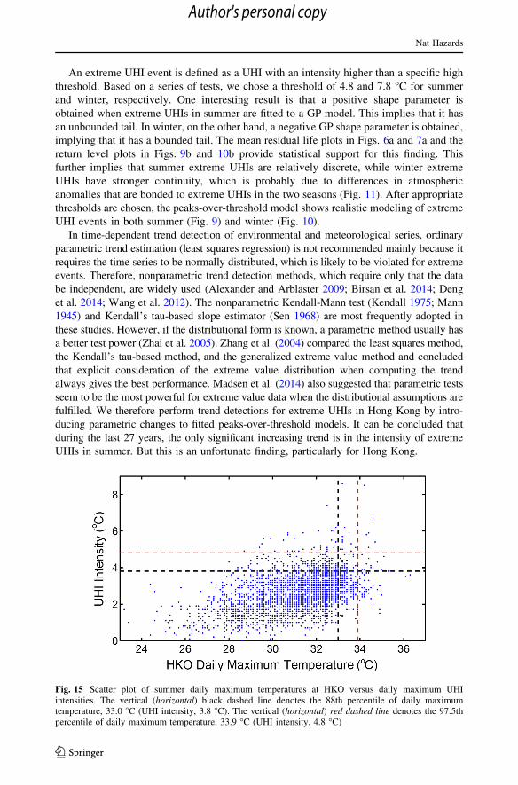
Fig. 15 Scatter plot of summer daily maximum temperatures at HKO versus daily maximum UHIintensities. The vertical (horizontal) black dashed line denotes the 88th percentile of daily maximumtemperature, 33.0 �C (UHI intensity, 3.8 �C). The vertical (horizontal) red dashed line denotes the 97.5thpercentile of daily maximum temperature, 33.9 �C (UHI intensity, 4.8 �C)
Nat Hazards
123
Author's personal copy

As a high-density city in the subtropics, Hong Kong is suffering from the ill effects of
UHIs due to land use, urbanization, and human activities. The old and the weak living in
their tiny rooms in urban areas will have to face an increasing number of hot nights with no
air conditioning (Lam 2006). What we have taken into account is the daily maximum UHI,
which usually occurs at nighttime. Meanwhile, extreme UHIs have a high possibility of
happening at a time when the background temperature is high, due to the synergistic
interactions between UHIs and heat waves, which has been found in other places (Li and
Bou-Zeid 2013; Li et al. 2015). For the case in Hong Kong, we demonstrate this possibility
simply by a scatter plot of daily maximum temperatures recorded at HKO versus daily
maximum UHI intensities (calculated from hourly temperatures) (Fig. 15). A hot day in
Hong Kong is commonly defined when the daily maximum temperature at HKO is above
33.0 �C, which is the 88th percentile of the data we utilized here (summer days during
1989–2015). The 88th percentile of summer UHI intensity is 3.8 �C. We can define this as
a lower criterion (black dashed lines in Fig. 15), while a higher criterion can be defined by
the 97.5th percentile (red dashed lines in Fig. 15). It is found that for the lower criterion,
the probability of extreme UHI occurrence is 10.5 % during nonhot days and increases to
32.3 % during hot days. For the higher criterion, the probability of extreme UHI occur-
rence is 2.4 % during nonhot days and increases to 11.5 % during hot days.
By synergy with summertime heat waves, UHIs can foster heat stress, creating a bio-
physical hazard (Zhou and Shepherd 2009). A significant increasing trend in the intensity
of extreme UHI events in summer implies that the risk of mortality and heat-related
diseases due to heat stress at night in summer, when the daily maximum UHI occurs, is
also increasing significantly. A study in Hong Kong has reported that a 1 �C rise in
physiological equivalent temperature may result in a 1.8 % increase in heat stress-related
mortality (Goggins et al. 2012). The warming climate has threatened and will continue to
threaten inhabitants in this subtropical high-density city. Strategies for mitigating human
impacts on the climate system during urban planning, such as adding greenery and plan-
ning a city with good natural ventilation, need to be implemented (Guindon and Nirupama
2015; Ng et al. 2011, 2012).
Because it is located in a subtropical coastal region, Hong Kong has a hot and humid
climate. Though UHIs in winter are stronger and their extreme events last longer than those
in summer, extreme UHIs in winter mean that it is warmer in the urban areas than in the
surrounding rural areas and this does not locally harm the inhabitants in the city. Fur-
thermore, extreme analysis detected no significant trends in wintertime extreme UHIs
(Fig. 13), which may relate to the significant decreasing trend of urban–rural precipitation
differences (Fig. 14).
Acknowledgments This study was supported by the Research Grants Council of the Hong Kong SpecialAdministrative Region (Project No. 14408214 and 11305715), City University of Hong Kong CampusSustainability Project (698603), and Institute of Environment, Energy and Sustainability, CUHK (ProjectID: 1907002). We thank the Hong Kong Observatory for providing meteorological records. We appreciatethe valuable comments and suggestions from the three anonymous reviewers.
References
Alexander LV, Arblaster JM (2009) Assessing trends in observed and modelled climate extremes overAustralia in relation to future projections. Int J Climatol 29:417–435
Birsan MV, Dumitrescu A, Micu DM, Cheval S (2014) Changes in annual temperature extremes in theCarpathians since AD 1961. Nat Hazards 74:1899–1910
Nat Hazards
123
Author's personal copy

Chan JCL, Zhou W (2005) PDO, ENSO and the early summer monsoon rainfall over south China. GeophysRes Lett 32:L08810. doi:10.1029/2004GL022015
Cheung HN, Zhou W, Mok HY, Wu MC, Shao Y (2013) Revisiting the climatology of atmospheric blockingin the Northern Hemisphere. Adv Atmos Sci 30:397–410
Cheung HN, Zhou W, S-m Lee, H-w Tong (2015) Interannual and interdecadal variability of the number ofcold days in Hong Kong and their relationship with large-scale circulation. Mon Weather Rev143:1438–1454
Coles S (2001) An introduction to statistical modeling of extreme values. Springer, LondonDeng H, Chen Y, Shi X, Li W, Wang H, Zhang S, Fang G (2014) Dynamics of temperature and precipitation
extremes and their spatial variation in the arid region of northwest China. Atmos Res 138:346–355Fung WY, Lam KS, Nichol J, Wong MS (2009) Derivation of nighttime urban air temperatures using a
satellite thermal image. J Appl Meteorol 48:863–872Furrer EM, Katz RW, Walter MD, Furrer R (2010) Statistical modeling of hot spells and heat waves. Clim
Res 43:191–205Garcia-Aristizabal A, Bucchignani E, Palazzi E, D’Onofrio D, Gasparini P, Marzocchi W (2014) Analysis of
non-stationary climate-related extreme events considering climate change scenarios: an application formulti-hazard assessment in the Dar es Salaam region, Tanzania. Nat Hazards 75:289–320
Giridharan R, Lau SSY, Ganesan S, Givoni B (2007) Urban design factors influencing heat island intensityin high-rise high-density environments of Hong Kong. Built Environ 42:3669–3684
Goggins WB, Chan E, Ng E, Ren C, Chen L (2012) Effect modification of the association between shortterm meteorological factors and mortality by urban heat islands in Hong Kong. PLoS One 7:e38551
Guindon S-M, Nirupama N (2015) Reducing risk from urban heat island effects in cities. Nat Hazards77:823–831
Habeeb D, Vargo J, Stone B (2015) Rising heat wave trends in large US cities. Nat Hazards 76:1651–1665Hondula DM, Davis RE (2014) The predictability of high-risk zones for heat-related mortality in seven US
cities. Nat Hazards 74:771–788IPCC (2013) Summary for Policymakers. In: Stocker TF, Qin D, Plattner GK, Tignor M, Allen SK,
Boschung J, Nauels A, Xia Y, Bex V, Midgley PM (eds) Climate change 2013: the physical sciencebasis contribution of working group I to the fifth assessment report of the intergovernmental panel onclimate change. Cambridge University Press, Cambridge
Kalnay E, Kanamitsu M, Kistler R et al (1996) The NCEP/NCAR 40-year reanalysis project. Bull AmMeteorol Soc 77:437–471
Kendall MG (1975) Rank correlation methods. Griffin, LondonKim D-W, Deo RC, Chung J-H, Lee J-S (2015) Projection of heat wave mortality related to climate change
in Korea. Nat Hazards. doi:10.1007/s11069-015-1987-0Lam CY (2006) On climate changes brought about by urban living. Hong Kong Meteorol Soc Bull 16:55–61Li D, Bou-Zeid E (2013) Synergistic interactions between urban heat islands and heat waves: the impact in
cities is larger than the sum of its parts. J Appl Meteorol 52:2051–2064Li D, Sun T, Liu M, Yang L, Wang L, Gao Z (2015) Contrasting responses of urban and rural surface energy
budgets to heat waves explain synergies between urban heat islands and heat waves. Environ Res Lett10:054009
Lilliefors HW (1967) On the Kolmogorov–Smirnov test for normality with mean and variance unknown.J Am Stat As 62:399–402
Liu L, Zhang Y (2011) Urban heat island analysis using the Landsat TM data and ASTER data: a case studyin Hong Kong. Remote Sens 3:1535–1552
Liu G, Zhang L, He B, Jin X, Zhang Q, Razafindrabe B, You H (2014) Temporal changes in extreme hightemperature, heat waves and relevant disasters in Nanjing metropolitan region, China. Nat Hazards76:1415–1430
Liu Y, Li S, Wang Y, Zhang T, Peng J, Li T (2015) Identification of multiple climatic extremes inmetropolis: a comparison of Guangzhou and Shenzhen, China. Nat Hazards 79:939–953
Madsen H, Lawrence D, Lang M, Martinkova M, Kjeldsen TR (2014) Review of trend analysis and climatechange projections of extreme precipitation and floods in Europe. J Hydrol 519:3634–3650
Mann HB (1945) Nonparametric trends against test. Econometrica 13:245–259Masek JG, Vermote EF, Saleous NE, Wolfe R, Hall FG, Huemmrich KF, Gao F, Kutler J, Lim TK (2006) A
Landsat surface reflectance data set for North America, 1990–2000. IEEE Geosci Remote Sens3:68–72
Massey FJ (1951) The Kolmogorov-Smirnov test for goodness of fit. J Am Stat As 46:68–78Memon RA, Leung DYC, Liu C (2008) A review on the generation, determination and mitigation of urban
heat island. J Environ Sci 20:120–128
Nat Hazards
123
Author's personal copy

Memon RA, Leung DYC, Liu C (2009) An investigation of urban heat island intensity (UHII) as anindicator of urban heating. Atmos Res 94:491–500
Ng E (2009) Policies and technical guidelines for urban planning of high-density cities: air ventilationassessment (AVA) of Hong Kong. Built Environ 44:1478–1488
Ng E, Yuan C, Chen L, Ren C, Fung JCH (2011) Improving the wind environment in high-density cities byunderstanding urban morphology and surface roughness: a study in Hong Kong. Landsc Urban Plan101:59–74
Ng E, Chen L, Wang Y, Yuan C (2012) A study on the cooling effects of greening in a high-density city: anexperience from Hong Kong. Built Environ 47:256–271
Oke TR (1982) The energetic basic of the urban heat island. Q J R Meteorol Soc 108:1–24Oke TR (1987) Boundary layer climates, 2nd edn. Routledge, LondonParey S, Hoang TTH (2015) Changes in the distribution of cold waves in France in the middle and end of the
21st century with IPSL-CM5 and CNRM-CM5 models. Clim Dyn. doi:10.1007/s00382-015-2877-6Qian C (2015) On trend estimation and significance testing for non-Gaussian and serially dependent data:
quantifying the urbanization effect on trends in hot extremes in the megacity of Shanghai. Clim Dyn.doi:10.1007/s00382-015-2838-0
Roth M (2007) Review of urban climate research in (sub)tropical regions. Int J Climatol 27:1859–1873Sen PK (1968) Estimates of the regression coefficient based on Kendall’s tau. J Am Stat As 63:1379–1389Sheridan SC, Kalkstein AJ, Kalkstein LS (2008) Trends in heat-related mortality in the United States,
1975–2004. Nat Hazards 50:145–160Shi J, Cui L (2011) Characteristics of high impact weather and meteorological disaster in Shanghai, China.
Nat Hazards 60:951–969Siu LW, Hart MA (2013) Quantifying urban heat island intensity in Hong Kong SAR, China. Environ Monit
Assess 185:4383–4398Smith RL (1989) Extreme value analysis of environmental time series: an application to trend detection in
ground-level ozone. Stat Sci 4:367–393Stanhill G, Kalma JD (1995) Solar dimming and urban heating at Hong Kong. Int J Climatol 15:933–941Wang H, Chen Y, Chen Z, Li W (2012) Changes in annual and seasonal temperature extremes in the arid
region of China, 1960–2010. Nat Hazards 65:1913–1930Wang W, Zhou W, Chen D (2014) Summer high temperature extremes in Southeast China: bonding with the
El Nino-Southern Oscillation and East Asian summer monsoon coupled system. J Clim 27:4122–4138Wang K, Li YG, Li YH, Yuan M (2015a) The stone forest as a small-scale field model for urban climate
studies. 9th International Conference on Urban Climate, 20th–24th July 2015, Toulouse, FranceWang W, Zhou W, Fong SK, Leong KC, Tang IM, Chang SW, Leong WK (2015b) Extreme rainfall and
summer heat waves in Macau based on statistical theory of extreme values. Clim Res 66:91–101Wang W, Zhou W, Li Y, Wang X, Wang D (2015c) Statistical modeling and CMIP5 simulations of hot spell
changes in China. Clim Dyn 44:2859–2872Wang W, Zhou W, Li X, Wang X, Wang D (2016) Synoptic-scale characteristics and atmospheric controls
of summer heat waves in China. Clim Dyn 46:2923–2941Wei K, Chen W, Zhou W (2011) Changes in the East Asian Cold Season since 2000. Adv Atmos Sci
28:69–79Xia J, Tu K, Yan Z, Qi Y (2015) The super-heat wave in eastern China during July-August 2013: a
perspective of climate change. Int J Climatol. doi:10.1002/joc.4424Yan ZW, Xia JJ, Qian C, Zhou W (2011) Changes in seasonal cycle and extremes in China during the period
1960–2008. Adv Atmos Sci 28:269–283Yim WWS, Ollier CD (2009) Managing planet earth to make future development more sustainable: climate
change and Hong Kong. Quat Sci 29:190–198Zhai PM, Zhang XB, Wan H, Pan XH (2005) Trends in total precipitation and frequency of daily precip-
itation extremes over China. J Clim 18:1096–1108Zhang XB, Zwiers FW, Li GL (2004) Monte Carlo experiments on the detection of trends in extreme values.
J Clim 17:1945–1952Zhao L, Lee X, Smith RB, Oleson K (2014) Strong contributions of local background climate to urban heat
islands. Nature 511:216–219Zhou Y, Shepherd JM (2009) Atlanta’s urban heat island under extreme heat conditions and potential
mitigation strategies. Nat Hazards 52:639–668Zhou W, Chan JCL, Chen W, Ling J, Pinto JG, Shao Y (2009) Synoptic-scale controls of persistent low
temperature and icy weather over southern China in January 2008. Mon Weather Rev 137:3978–3991Zhou D, Zhao S, Zhang L, Sun G, Liu Y (2015) The footprint of urban heat island effect in China. Sci Rep
5:11160
Nat Hazards
123
Author's personal copy
Recommended