Uncertainty in multiphase flow estimates for a field development case
Ingvil Bjørlo
Master of Science in Engineering and ICT
Supervisor: Ole Jørgen Nydal, EPTCo-supervisor: Peter Sassan Johansson, Statoil ASA
Bjørnar Hauknes Pettersen, Statoil ASA
Department of Energy and Process Engineering
Submission date: June 2013
Norwegian University of Science and Technology


Uncertainty in multiphase flow estimates for a field development case
Classification: Internal i
Sammendrag
Kommersielle flerfasesimulatorer gir vanligvis én verdi for hver outputparameter som blir
simulert i en rørledning. Prosjektledere for feltutbygging vil vite usikkerheten i disse
prediksjonene for å vurdere risikoen. To feltstudier fra rørledningen P10 fra Troll plattformen ble
undersøkt; ett tilfelle var tyngdekraftsdominert og det andre var friksjonsdominert. Dette ble
gjennomført ved å bruke flerfasesimulatoren OLGA og funksjoner i den innebygde RMO (Risk
Management and Optimization) modulen.
En sensitivitetsanalyse ble utført for å undersøke den lineære effekten av input- og
modellparameterne på outputparameterne, og de mest betydningsfulle parameterne ble funnet.
For å se simultane effekter ble en usikkerhetsanalyse utført. Latin Hypercube metoden ble brukt
til å finne et utvalg ved å trekke input- og modellparametere i henhold til en
sannsynlighetsfordeling, og deretter beregne outputverdier. Ut i fra dette ble usikkerhets-
intervaller funnet for outputparameterne. Resultatene ble deretter sammenlignet med målinger
fra Troll-feltet, for å se hvor godt OLGA klarte å simulere rørledningen. En tuning ble utført for
å se om beregningene kom nærmere målingene ved å endre noen av modellparametere. Dette
viste seg å være utfordrende ettersom rørledningen har lav væskelast og stiger i en veldig bratt
vinkel mot land.
Som en metode for usikkerhetsestimering av resultater fra flerfasesimulering har RMO modulen
potensial til å være et nyttig og praktisk verktøy. For øyeblikket har det imidlertid for mye
uberegnelige oppførsel som fører til tap av data og tid. Generelt var denne typen metodikk for
usikkerhetsestimering svært nyttig for å visualisere flerfasetransportrisiko i forbindelse med en
feltutbygging, og representerer et betydelig skritt fremover i så måte.
Uncertainty in multiphase flow estimates for a field development case
Classification: Internal ii
Abstract
Commercial multiphase flow simulators typically give one value for each output parameter
simulated in a pipeline. Field development project managers want to know the uncertainty in
these predictions in order to assess the risk. A study on two field cases, one gravity dominated
case and one friction dominated, from the Troll P10 pipeline was conducted using the multiphase
flow simulator OLGA and the functions in the embedded RMO (Risk Management and
Optimization) module.
A sensitivity analysis was performed to investigate the linear effects of the input- and model
parameters on the output, and the most influential parameters were found. To see simultaneous
effects, an uncertainty analysis was executed, drawing input- and model parameter values using
Latin Hypercube sampling according to a probability distribution, and calculating the output
values. Thus, uncertainty ranges were found for the output parameters. The results were then
compared to measurements from the Troll field, to see how well OLGA simulated the pipeline.
A tuning session was performed to see if the calculations were closer to the measurements when
altering some of the model parameters. This proved challenging, as the pipeline has low liquid
loading and a high pipe inclination towards land.
As a methodology for uncertainty estimation of multiphase simulation results, the RMO module
has potential to be a useful and practical tool. However, it currently has too much erratic
behavior which causes loss of data and time. Generally, this sort of uncertainty estimation
methodology was very useful to visualize flow assurance risk in connection with a field
development project, and represents a significant step forward in this regard.

Uncertainty in multiphase flow estimates for a field development case
Classification: Internal iii
Preface
This report is a result of cooperation between me, student technician Ingvil Bjørlo, writing a
master thesis for the Norwegian University of Science and Technology and Statoil ASA. I came
in contact with the Statoil Research Centre in Trondheim when I applied for a summer internship
through professor Ole Jørgen Nydal and his multiphase flow course at NTNU. I continued
working with Statoil after the internship, and completed my project thesis the following
semester. This last semester has been spent on my master thesis, and I have enjoyed working
almost a year with Statoil.
Multiphase flow is a complex and challenging field of study and it has been very rewarding for
me to learn more about it from experienced people. With my background in computing and ICT,
it has also been very interesting to work with multiphase flow simulators.
I would like to thank Peter Sassan Johansson, Bjørnar Hauknes Pettersen and Zhilin Yang at
Statoil ASA and Ole Jørgen Nydal at NTNU for valuable help and guidance throughout this
project. Especially Dr. Johansson has spent a lot of time with me, patiently answering questions
and giving useful feedback, which I am very grateful for. I would also like to thank Statoil ASA
for access to their offices at Rotvoll for the duration of the project and for providing licenses and
software needed to complete the work for this thesis.
Ingvil Bjørlo, June 4, 2013. Trondheim
Uncertainty in multiphase flow estimates for a field development case
Classification: Internal iv
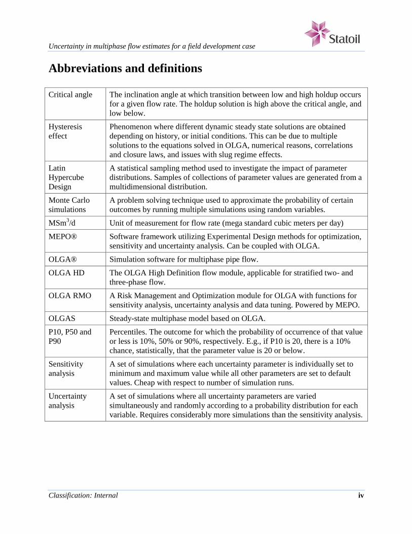
Abbreviations and definitions
Critical angle The inclination angle at which transition between low and high holdup occurs
for a given flow rate. The holdup solution is high above the critical angle, and
low below.
Hysteresis
effect
Phenomenon where different dynamic steady state solutions are obtained
depending on history, or initial conditions. This can be due to multiple
solutions to the equations solved in OLGA, numerical reasons, correlations
and closure laws, and issues with slug regime effects.
Latin
Hypercube
Design
A statistical sampling method used to investigate the impact of parameter
distributions. Samples of collections of parameter values are generated from a
multidimensional distribution.
Monte Carlo
simulations
A problem solving technique used to approximate the probability of certain
outcomes by running multiple simulations using random variables.
MSm3/d Unit of measurement for flow rate (mega standard cubic meters per day)
MEPO® Software framework utilizing Experimental Design methods for optimization,
sensitivity and uncertainty analysis. Can be coupled with OLGA.
OLGA® Simulation software for multiphase pipe flow.
OLGA HD The OLGA High Definition flow module, applicable for stratified two- and
three-phase flow.
OLGA RMO A Risk Management and Optimization module for OLGA with functions for
sensitivity analysis, uncertainty analysis and data tuning. Powered by MEPO.
OLGAS Steady-state multiphase model based on OLGA.
P10, P50 and
P90
Percentiles. The outcome for which the probability of occurrence of that value
or less is 10%, 50% or 90%, respectively. E.g., if P10 is 20, there is a 10%
chance, statistically, that the parameter value is 20 or below.
Sensitivity
analysis
A set of simulations where each uncertainty parameter is individually set to
minimum and maximum value while all other parameters are set to default
values. Cheap with respect to number of simulation runs.
Uncertainty
analysis
A set of simulations where all uncertainty parameters are varied
simultaneously and randomly according to a probability distribution for each
variable. Requires considerably more simulations than the sensitivity analysis.

Uncertainty in multiphase flow estimates for a field development case
Classification: Internal Page 1 of 77
Table of Contents
Sammendrag ................................................................................................................................... i
Abstract .......................................................................................................................................... ii
Preface ........................................................................................................................................... iii
Abbreviations and definitions ..................................................................................................... iv
1 Introduction ........................................................................................................................... 4
1.1 Background ..................................................................................................................... 4
1.2 Objective ......................................................................................................................... 4
2 Literature review .................................................................................................................. 5
2.1 Uncertainty estimates in multiphase flow simulation, SPT Group 2012 ........................ 5
2.2 Shtokman flow assurance uncertainty analysis, SPT Group 2011 ................................. 8
2.3 Conclusion .................................................................................................................... 10
3 Background theory ............................................................................................................. 12
3.1 Field cases: Troll P10 pipeline ...................................................................................... 12
3.2 OLGA Risk Management and Optimization module ................................................... 15
3.3 Latin Hypercube Sampling ........................................................................................... 16
4 Methodology ........................................................................................................................ 17
5 Parameter selection, ranges, and distribution functions ................................................. 19
5.1 Field case: Troll P10 pipeline, 34.9 MSm3/d ................................................................ 21
5.2 Field case: Troll P10 pipeline, 24.6 MSm3/d ................................................................ 23
6 Results and analysis ............................................................................................................ 25
6.1 Field case: Troll P10 pipeline, 34.9 MSm3/d ................................................................ 25
6.1.1 Sensitivity analysis .................................................................................................... 25
6.1.2 Uncertainty analysis ................................................................................................. 32
6.1.3 Tuning ....................................................................................................................... 39
6.2 Field case: Troll P10 pipeline, 24.6 MSm3/d ................................................................ 41
6.2.1 Sensitivity analysis .................................................................................................... 41
6.2.2 Uncertainty analysis ................................................................................................. 48
6.2.3 Tuning ....................................................................................................................... 55
7 Discussion............................................................................................................................. 57
7.1 On using the RMO module for uncertainty estimation ................................................. 57
7.2 On the results ................................................................................................................ 58

Uncertainty in multiphase flow estimates for a field development case
Classification: Internal Page 2 of 77
8 Conclusion ........................................................................................................................... 62
9 Recommendations for further work.................................................................................. 63
10 References ............................................................................................................................ 64
11 Appendices ........................................................................................................................... 65
11.1 Appendix A – Scatter plots from the uncertainty analyses ........................................... 65
11.2 Appendix B – Plots from the tuning sessions ............................................................... 69
List of figures
Figure 3-1: The Troll field with approximate locations of the platforms ..................................... 12
Figure 3-2: Flow chart Troll A - Kollsnes .................................................................................... 12
Figure 3-3: Profile plot of the P10 pipeline geometry from OLGA ............................................. 14
Figure 3-4: Overview of the workflow in OLGA/RMO ............................................................... 15
Figure 3-5: Latin square example ................................................................................................. 16
Figure 5-1: Triangular distribution example ................................................................................. 21
Figure 6-1: Tornado plot for total pressure drop P10 pipeline, 34.9 MSm3/d .............................. 26
Figure 6-2: Tornado plot for pressure at inlet P10 pipeline, 34.9 MSm3/d .................................. 27
Figure 6-3: Tornado plot for total liquid content P10 pipeline, 34.9 MSm3/d.............................. 28
Figure 6-4: Tornado plot for total oil content P10 pipeline, 34.9 MSm3/d ................................... 29
Figure 6-5: Tornado plot for total water content P10 pipeline, 34.9 MSm3/d .............................. 30
Figure 6-6: Distribution plot for total pressure drop, P10 pipeline, 34.9 MSm3/d ....................... 33
Figure 6-7: Distribution plot for inlet pressure, P10 pipeline, 34.9 MSm3/d................................ 34
Figure 6-8: Distribution plot for total liquid content, P10 pipeline, 34.9 MSm3/d ....................... 35
Figure 6-9: Distribution plot for total oil content, P10 pipeline, 34.9 MSm3/d ............................ 36
Figure 6-10: Distribution plot for total water content, P10 pipeline, 34.9 MSm3/d ..................... 37
Figure 6-11: Tornado plot for total pressure drop P10 pipeline, 24.6 MSm3/d ............................ 42
Figure 6-12: Tornado plot for pressure at inlet P10 pipeline, 24.6 MSm3/d ................................ 43
Figure 6-13: Tornado plot for total liquid content P10 pipeline, 24.6 MSm3/d............................ 44
Figure 6-14: Tornado plot for total oil content P10 pipeline, 24.6 MSm3/d ................................. 45
Figure 6-15: Tornado plot for total water content P10 pipeline, 24.6 MSm3/d ............................ 46
Figure 6-16: Distribution plot for total pressure drop, P10 pipeline, 24.6 MSm3/d ..................... 49
Figure 6-17: Distribution plot for inlet pressure, P10 pipeline, 24.6 MSm3/d.............................. 50
Figure 6-18: Distribution plot for total liquid content, P10 pipeline, 24.6 MSm3/d ..................... 51
Figure 6-19: Distribution plot for total oil content, P10 pipeline, 24.6 MSm3/d .......................... 52
Figure 6-20: Distribution plot for total water content, pipeline, 24.6 MSm3/d ............................ 53

Uncertainty in multiphase flow estimates for a field development case
Classification: Internal Page 3 of 77
List of tables
Table 2-1: SPT Group 2012 - List of input parameters .................................................................. 5
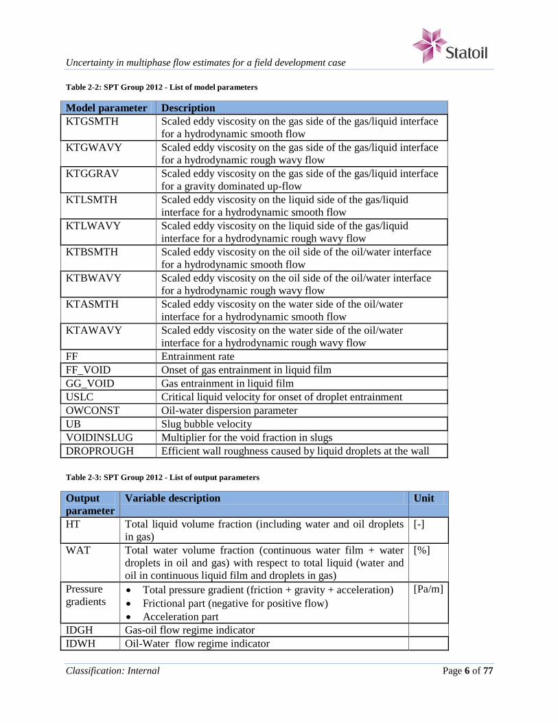
Table 2-2: SPT Group 2012 - List of model parameters ................................................................ 6
Table 2-3: SPT Group 2012 - List of output parameters ................................................................ 6
Table 2-4: SPT Group 2012 - Range and distribution functions from tuning against two-phase
measurements .................................................................................................................................. 7
Table 2-5: SPT Group 2012 - Range and distribution functions from tuning against three-
phase measurements........................................................................................................................ 7
Table 2-6: SPT Group 2011 – List of input parameters with ranges .............................................. 9
Table 2-7: SPT Group 2011 – List of model parameters with ranges ............................................ 9
Table 2-8: SPT Group 2011 - Additional parameters for dynamic simulations ........................... 10
Table 3-1: Results from Troll tests by Statoil ............................................................................... 13
Table 5-1: Input-, model- and output parameters to be tested for the P10 pipeline ..................... 19
Table 5-2: Inlet conditions for the P10 pipeline, 34.9 MSm3/d .................................................... 22
Table 5-3: Ranges and distribution functions for input- and model parameters to be tested for
the P10 pipeline, 34.9 MSm3/d ..................................................................................................... 22
Table 5-4: Inlet conditions for the P10 pipeline, 24.6 MSm3/d .................................................... 23
Table 5-5: Ranges and distribution functions for input- and model parameters to be tested for
the P10 pipeline, 24.6 MSm3/d ..................................................................................................... 23
Table 6-1: Results from OLGA simulations ................................................................................. 25
Table 6-2: Summary of results from sensitivity analysis, 34.9 MSm3/d ...................................... 31
Table 6-3: Summary of results from uncertainty analysis, 34.9 MSm3/d ..................................... 38
Table 6-4: Comparison with Troll measurement data, 34.9 MSm3/d ........................................... 39
Table 6-5: Tuned parameters, 34.9 MSm3/d ................................................................................. 39
Table 6-6: Summary of results from tuning, 34.9 MSm3/d .......................................................... 40
Table 6-7: Comparison of tuning with Troll measurement data, 34.9 MSm3/d ........................... 40
Table 6-8: Summary of results from sensitivity analysis, 24.6 MSm3/d ...................................... 47
Table 6-9: Summary of results from uncertainty analysis, 24.6 MSm3/d ..................................... 54
Table 6-10: Comparison with Troll measurement data, 24.6 MSm3/d ......................................... 55
Table 6-11: Summary of results from tuning, 24.6 MSm3/d ........................................................ 56
Table 6-12: Comparison of tuning with Troll measurement data, 24.6 MSm3/d ......................... 56

Uncertainty in multiphase flow estimates for a field development case
Classification: Internal Page 4 of 77
1 Introduction
1.1 Background
A commercial multiphase flow simulator will typically give one value for the required inlet
pressure and the accumulated liquid in the pipeline for a given flow rate. There is, however,
considerable uncertainty both in the model parameters used in the flow model and in the input
parameters given by the user, which can give considerable uncertainty for the output parameters.
Field development project managers want to know the uncertainty in the predictions in order to
assess the risk, i.e. the potential severity of impact. Identifying uncertainty and its control has
become a focus area in the oil and gas industry. Two field cases from a Troll pipeline have been
selected for the study; one is gravity dominated and the other is friction dominated.
The basis for the work will be the commercial flow simulator OLGA 7 with the Risk
Management and Optimization (RMO) module. MEPO is a program currently used for
uncertainty estimation, among other things, but it is quite extensive and requires its own license.
The RMO module is a less extensive version of MEPO embedded in OLGA. It is therefore of
interest to investigate the RMO module and whether or not it is an adequate alternative for
uncertainty estimation. In the RMO module, input parameters and important model parameters
may be given a probability distribution function with assigned upper and lower limits. A
statistical sampling method can then randomly draw values between these limits, and the RMO
module will then provide a probability distribution of the output variables such as inlet pressure
and accumulated liquid. Thus, an uncertainty band for the output variables can be found, and the
risk can be assessed.
1.2 Objective
A methodology for uncertainty estimation of multiphase simulation results is to be developed.
The following tasks are to be considered:
1. A short literature study on internal work performed by subcontractor and Statoil
2. Familiarisation of the OLGA program and the use of the RMO module
3. Construction and modification of an OLGA model for two selected field cases
4. Evaluate input- and model parameter uncertainty spans and probability distributions
5. Perform uncertainty analyses, evaluate the results, and iterate on point 4 if necessary
6. Assess the performance of the RMO module
7. Present the results in a report with suggestions for further work

Uncertainty in multiphase flow estimates for a field development case
Classification: Internal Page 5 of 77
2 Literature review
Some internal work concerning uncertainty analysis of input- and model parameters has already
been performed by subcontractor and Statoil ASA. These reports indicate which parameters are
deemed important for the uncertainty estimation, and how the previous work has been executed.
The work found most relevant for this study is summarized below.
2.1 Uncertainty estimates in multiphase flow simulation, SPT Group 2012
SPT Group did some work for Statoil looking for a universal and structured method to specify
flow model uncertainties (Kirkedelen, 2012). An experimental matrix with 10 000 different
combinations of input parameters was provided by Statoil, based on Statoil’s database of
laboratory measurements. The commercial flow simulator OLGAS (OLGA steady-state) with the
High Definition (HD) model was used for the calculations. The model parameters were identified
through discussions with the model development groups at SPT Group and IFE. An overview of
the parameters used is found in Table 2-1, Table 2-2 and Table 2-3 (Kirkedelen, 2012, pp. ii -
iii).
Table 2-1: SPT Group 2012 - List of input parameters
Input
parameter
Description Unit Comments
USG Superficial velocity gas [m/s] Parameter ending = A:
Absolute uncertainty
(e.g. USGA, USHA,
etc.)
Parameter ending = R:
Relative uncertainty
(e.g. USGR, USHR,
etc.)
USH Superficial velocity oil [m/s]
USW Superficial velocity water [m/s]
ROG Density oil [kg/m3]
ROH Density gas [kg/m3]
ROW Density water [kg/m3]
MUG Viscosity gas [Pa∙s]
MUH Viscosity oil [Pa∙s]
MUW Viscosity water [Pa∙s]
SIGGH Interfacial tension gas-oil [N/m]
SIGGW Interfacial tension gas-water [N/m]
SIGHW Interfacial tension oil-water [N/m]
DIAMA Pipe diameter [m] Absolute uncertainty
PHI1A Pipe inclination [°] Absolute uncertainty
EPSABSR Pipe roughness [m] Relative uncertainty
Uncertainty in multiphase flow estimates for a field development case
Classification: Internal Page 6 of 77
Table 2-2: SPT Group 2012 - List of model parameters
Model parameter Description
KTGSMTH Scaled eddy viscosity on the gas side of the gas/liquid interface
for a hydrodynamic smooth flow
KTGWAVY Scaled eddy viscosity on the gas side of the gas/liquid interface
for a hydrodynamic rough wavy flow
KTGGRAV Scaled eddy viscosity on the gas side of the gas/liquid interface
for a gravity dominated up-flow
KTLSMTH Scaled eddy viscosity on the liquid side of the gas/liquid
interface for a hydrodynamic smooth flow
KTLWAVY Scaled eddy viscosity on the liquid side of the gas/liquid
interface for a hydrodynamic rough wavy flow
KTBSMTH Scaled eddy viscosity on the oil side of the oil/water interface
for a hydrodynamic smooth flow
KTBWAVY Scaled eddy viscosity on the oil side of the oil/water interface
for a hydrodynamic rough wavy flow
KTASMTH Scaled eddy viscosity on the water side of the oil/water
interface for a hydrodynamic smooth flow
KTAWAVY Scaled eddy viscosity on the water side of the oil/water
interface for a hydrodynamic rough wavy flow
FF Entrainment rate
FF_VOID Onset of gas entrainment in liquid film
GG_VOID Gas entrainment in liquid film
USLC Critical liquid velocity for onset of droplet entrainment
OWCONST Oil-water dispersion parameter
UB Slug bubble velocity
VOIDINSLUG Multiplier for the void fraction in slugs
DROPROUGH Efficient wall roughness caused by liquid droplets at the wall
Table 2-3: SPT Group 2012 - List of output parameters
Output
parameter
Variable description Unit
HT Total liquid volume fraction (including water and oil droplets
in gas)
[-]
WAT Total water volume fraction (continuous water film + water
droplets in oil and gas) with respect to total liquid (water and
oil in continuous liquid film and droplets in gas)
[%]
Pressure
gradients Total pressure gradient (friction + gravity + acceleration)
Frictional part (negative for positive flow)
Acceleration part
[Pa/m]
IDGH Gas-oil flow regime indicator
IDWH Oil-Water flow regime indicator
Uncertainty in multiphase flow estimates for a field development case
Classification: Internal Page 7 of 77
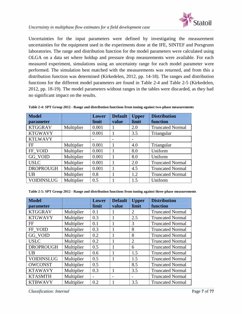
Uncertainties for the input parameters were defined by investigating the measurement
uncertainties for the equipment used in the experiments done at the IFE, SINTEF and Porsgrunn
laboratories. The range and distribution function for the model parameters were calculated using
OLGA on a data set where holdup and pressure drop measurements were available. For each
measured experiment, simulations using an uncertainty range for each model parameter were
performed. The simulation best matched with the measurements was returned, and from this a
distribution function was determined (Kirkedelen, 2012, pp. 14-18). The ranges and distribution
functions for the different model parameters are found in Table 2-4 and Table 2-5 (Kirkedelen,
2012, pp. 18-19). The model parameters without ranges in the tables were discarded, as they had
no significant impact on the results.
Table 2-4: SPT Group 2012 - Range and distribution functions from tuning against two-phase measurements
Model
parameter
Lower
limit
Default
value
Upper
limit
Distribution
function
KTGGRAV Multiplier 0.001 1 2.0 Truncated Normal
KTGWAVY 0.001 1 3.5 Triangular
KTLWAVY - - -
FF Multiplier 0.001 1 4.0 Triangular
FF_VOID Multiplier 0.001 1 8.0 Uniform
GG_VOID Multiplier 0.001 1 8.0 Uniform
USLC Multiplier 0.001 1 2.0 Truncated Normal
DROPROUGH Multiplier 0.001 1 4.5 Truncated Normal
UB Multiplier 0.8 1 1.2 Truncated Normal
VOIDINSLUG Multiplier 0.5 1 1.5 Uniform
Table 2-5: SPT Group 2012 - Range and distribution functions from tuning against three-phase measurements
Model
parameter
Lower
limit
Default
value
Upper
limit
Distribution
function
KTGGRAV Multiplier 0.1 1 2 Truncated Normal
KTGWAVY Multiplier 0.3 1 2.5 Truncated Normal
FF Multiplier 0.1 1 3 Truncated Normal
FF_VOID Multiplier 0.3 1 8 Truncated Normal
GG_VOID Multiplier 0.2 1 8 Truncated Normal
USLC Multiplier 0.2 1 2 Truncated Normal
DROPROUGH Multiplier 0.5 1 6 Truncated Normal
UB Multiplier 0.6 1 1.5 Truncated Normal
VOIDINSLUG Multiplier 0.5 1 1.5 Truncated Normal
OWCONST Multiplier 0.5 8.5 Truncated Normal
KTAWAVY Multiplier 0.3 1 3.5 Truncated Normal
KTASMTH Multiplier - - - Truncated Normal
KTBWAVY Multiplier 0.2 1 3.5 Truncated Normal

Uncertainty in multiphase flow estimates for a field development case
Classification: Internal Page 8 of 77
Model
parameter
Lower
limit
Default
value
Upper
limit
Distribution
function
KTBSMTH Multiplier - - -
KTLWAVY Multiplier - - -
KTLSMTH Multiplier - - -
KTGSMTH Multiplier - - -
A sensitivity analysis was performed in the analysis and optimization framework called MEPO
to see the linear sensitivities of the output parameters to the input- and model parameters, thus
finding the parameters which are most important. Then, an uncertainty analysis was performed in
MEPO using the Latin Hypercube sampling method. The output parameters were calculated
while each uncertainty parameter was randomly varied between the minimum and maximum
values according to the given probability distribution function. Thus, an uncertainty span
between P10 and P90 values could be found for the output parameters.
2.2 Shtokman flow assurance uncertainty analysis, SPT Group 2011
SPT Group has also performed a set of analyses for the Shtokman field in the Barents Sea. The
first part was a core model evaluation, where the goal was to find the best OLGA model to use
for the Shtokman flow assurance uncertainty analysis (Vanvik, 2011). A set of OLGA flow
models at conditions relevant for two-phase transfer of gas and condensate from the Shtokman
field to shore were evaluated. Comparisons with relevant laboratory- and field data were
performed. The OLGA HD model was found to have the best overall match for both field- and
experimental data. In addition, OLGA HD had no discontinuity in predicted critical angle versus
flow rate, and the problems related to liquid holdup hysteresis during ramp-down/ramp-up were
significantly reduced.
The second part consisted of developing and applying a methodology for a risk based uncertainty
analysis of steady state prediction of pressure drop, capacity, minimum turndown and liquid
content for the Shtokman long dry two-phase flow trunk lines to shore (Vanvik, Biberg, Holm, &
Hoyer, 2011). The methodology proved to be successful, and the results seemed to be applicable.
The Shtokman flow line was simulated using the OLGA HD 7.0.0 flow model coupled with
MEPO. The uncertainty parameters considered in this study can be found in Table 2-6 and Table
2-7 (Vanvik, Biberg, Holm, & Hoyer, 2011, pp. 17, 21.).

Uncertainty in multiphase flow estimates for a field development case
Classification: Internal Page 9 of 77
Table 2-6: SPT Group 2011 – List of input parameters with ranges
Input parameter Description Found in Lower
limit
Default
value
Upper
limit
LIQHCFAC Liquid hydrocarbon
fraction
TUNING 0.4 1 1.76
GASDENSITY Gas density TUNING 0.95 1 1.05
OILDENSITY Oil density TUNING 0.9 1 1.1
GASVISC Gas viscosity TUNING 0.9 1 1.1
OILVISC Oil viscosity TUNING 0.7 1 1.3
SIGGL Gas/liquid surface tension TUNING 0.5 1 1.5
ROUGHNESS Hydraulic wall roughness
(μm)
PIPE 0 30 46
XSTART Flowline length (km) GEOMETRY 0 0 +5
DIAMETER Internal diameter (mm) PIPE 862.4 863.4 864.4
PRESSURE Arrival pressure (bara) NODE 60 60 70
UVALUE Heat transfer coefficient
(W/m2/K)
HEATTRANSFER 10 18 30
OUTTAMBIENT
and TAMBIENT
Seawater temperature (°C) HEATTRANSFER -2 -1.8 4
Trunk line
geometry
Three different elevation
profiles
(1=worst, 2=base,
3=best)
1 2 3
Table 2-7: SPT Group 2011 – List of model parameters with ranges
Model parameter Description Found in Lower
limit
Default
value
Upper
limit
DIAMPOWER Diameter exponent TUNING 0.5 1 1.5
ANGLESCALE Inclination term factor TUNING 0 1 3
ANGLEDIAMPOWER Inclination term exponent TUNING 0 0 1.5
GROUGHNESS Roughness effect of droplets TUNING 0.7 1 1.3
WETFRACTION Scaling of droplet wetted
wall
TUNING 0.7 1 1.3
KTGSMTHFAC Smooth turbulence for gas TUNING 0.7 1 1.3
KTGWAVYFAC Wavy turbulence for gas TUNING 0.7 1 1.3
KTGGRAVFAC Gravity turbulence for gas TUNING 0.7 1 1.3
KTALOWTFAC Low turbulence for liquid TUNING 0.7 1 1.3
KTAHIGHTFAC High turbulence for liquid TUNING 0.7 1 1.3
A sensitivity analysis was then performed in MEPO to investigate which uncertainty parameters
had the most influence on the liquid content at low flow rate, pressure drop at design flow rate,
and arrival temperature at design flow rate. Parameters that had no effect at all were
KTGSMTHFAC, GROUGHNESS and WETFRACTION. However, it was assumed that the

Uncertainty in multiphase flow estimates for a field development case
Classification: Internal Page 10 of 77
effect could be present when varying all input- and model parameters simultaneously. In order to
capture nonlinear dependence of the input- and model parameters, an uncertainty analysis was
performed in MEPO using the Latin Hypercube sampling method. In this case, a triangular
distribution was chosen for all parameters, ensuring that a significant fraction of the parameter
values would be close to the upper and lower limits. In such a way, uncertainty spans for the
liquid content, required inlet pressure and pressure drop were obtained.
The third part of SPT Group’s analyses was developing and applying a methodology for a risk
based uncertainty analysis of dynamic simulations of production ramp-up for the Shtokman long
dry two-phase flow trunk lines to shore (Vanvik & Holm, 2011). However, the simulation cost
associated with transient simulations of the Shtokman flowlines makes such an approach very
challenging. The uncertainty parameters used were the same as for the previous steady-state from
WPII, in addition to two new parameters, seen in Table 2-8.
Table 2-8: SPT Group 2011 - Additional parameters for dynamic simulations
Uncertainty
parameters
Description Lower
limit
Default
value
Upper
limit
Found in
Ramp-up
time (TIME)
Time taken for the flow rate at inlet
to be increased from initial to final
value (h)
1 6 24 SOURCE
Drainage
capacity
The maximum volumetric liquid
flow rate that must be drained from
the slug catcher (m3/h)
- 76 - Post-
processing
The methodology for the uncertainty analysis is much the same as for the steady-state study. As
dynamic situations are not part of the scope for this work, the information from this report is not
relevant in this case.
2.3 Conclusion
In both these sets of reports, OLGA HD 7.0.0 was used to perform the simulations. The scope of
this project is for steady-state, and dynamic situations will not be taken into account. Hence,
OLGA HD 7.1.4 (the latest version available in Statoil) with the steady-state option will be used
for the simulation of the selected field cases in this project. More information about the field
cases can be found in chapter 3.1.

Uncertainty in multiphase flow estimates for a field development case
Classification: Internal Page 11 of 77
The execution of the analyses was similar in the reports:
1. OLGA simulation of data
2. Sensitivity analysis by coupling OLGA with MEPO
3. Uncertainty analysis by coupling OLGA with MEPO
4. Analysis of the obtained results, and further tuning if necessary
The process can be used similarly in this study, except for the use of the MEPO software. After
simulating the field cases in OLGA, the sensitivity and uncertainty analyses in this project will
be performed using the RMO module embedded in OLGA 7.1.4. The RMO module does not
have all the functions MEPO has, but it is powered by MEPO, and the analyses will thus be
similar. More information about the RMO module can be found in chapter 3.2.
In the first report (Kirkedelen, 2012), the uncertainty analysis was based on experimental data
from Statoil’s laboratory database. The experimental data were entered into OLGA and
simulated, and could then be analyzed by coupling OLGA with MEPO. The Shtokman
uncertainty analysis (Vanvik, Biberg, Holm, & Hoyer, 2011), was based on an OLGA simulation
of the Shtokman flowline, and was also done through MEPO. Both reports have their own list of
input- and model parameters, with their respective upper and lower limits, and distribution
functions. These parameters are the ones deemed important by the OLGA developers in SPT
Group. The same input- and model parameters are tested in this project as well. Some of the
parameters are not available for regular users of OLGA, i.e. they are not available from the
commercial OLGA graphical user interface.
The field cases to be considered in this study are three-phase flows; hence the upper and lower
limits used for analyses should essentially be taken from the three-phase results. The Shtokman
flow line study assumed two-phase flow, but the limits from field data may be more relevant
than the limits from experimental data. Therefore, if there are no three-phase parameter limits,
the Shtokman parameter limits are used in this study.
The original idea was to use a Monte Carlo sampling method to generate samples for the
uncertainty analysis. However, as seen in these reports, MEPO (and hence the RMO module) has
Latin Hypercube sampling embedded. While Monte Carlo generates samples randomly, the Latin
Hypercube method ensures that no sample can be selected twice. Thus, Latin Hypercube
sampling will span the sample space with fewer samples. It was therefore decided that Latin
Hypercube sampling should be used instead of the Monte Carlo simulations for this project.
More information about Latin Hypercube sampling can be found in chapter 3.3.
Uncertainty in multiphase flow estimates for a field development case
Classification: Internal Page 12 of 77
3 Background theory
3.1 Field cases: Troll P10 pipeline
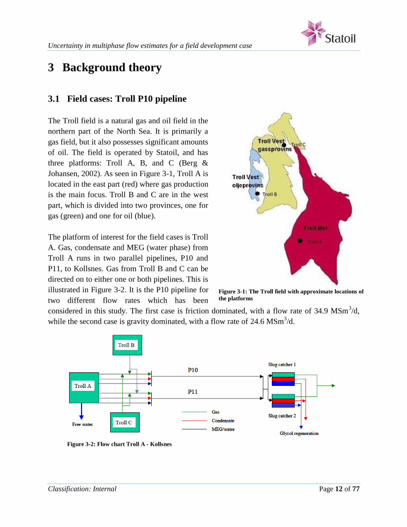
The Troll field is a natural gas and oil field in the
northern part of the North Sea. It is primarily a
gas field, but it also possesses significant amounts
of oil. The field is operated by Statoil, and has
three platforms: Troll A, B, and C (Berg &
Johansen, 2002). As seen in Figure 3-1, Troll A is
located in the east part (red) where gas production
is the main focus. Troll B and C are in the west
part, which is divided into two provinces, one for
gas (green) and one for oil (blue).
The platform of interest for the field cases is Troll
A. Gas, condensate and MEG (water phase) from
Troll A runs in two parallel pipelines, P10 and
P11, to Kollsnes. Gas from Troll B and C can be
directed on to either one or both pipelines. This is
illustrated in Figure 3-2. It is the P10 pipeline for
two different flow rates which has been
considered in this study. The first case is friction dominated, with a flow rate of 34.9 MSm3/d,
while the second case is gravity dominated, with a flow rate of 24.6 MSm3/d.
Figure 3-2: Flow chart Troll A - Kollsnes
Figure 3-1: The Troll field with approximate locations of
the platforms

Uncertainty in multiphase flow estimates for a field development case
Classification: Internal Page 13 of 77
Table 3-1: Results from Troll tests by Statoil
Test 7
August 2002
Test 8
April 2004
Gas flow rate 24.61 MSm3/d 34.94 MSm
3/d
Condensate
Flow rate
Density
2.87 m3/h
700.3 kg/m3
0 m3/h
700.3 kg/m3
MEG
Flow rate
Density
3.9 m3/h
1086 kg/m3
3.8 m3/h
1086 kg/m3
Troll A gas
Flow rate
Temperature
Density
20.04 MSm3/d
37.3 °C
0.739 kg/m3
34.94 MSm3/d
44.6 °C
0.739 kg/m3
Troll B gas
Flow rate
Temperature
Density
4.57 MSm3/d
4.58 °C
0.789 kg/m3
0 MSm3/d
5 °C
0.789 kg/m3
Troll C gas
Flow rate
Temperature
Density
0 MSm3/d
5 °C
0.776 kg/m3
0 MSm3/d
5 °C
0.776 kg/m3
Mass flow rate
Gas 213.1 kg/s 298.9 kg/s
Condensate 0.558 kg/s 0 kg/s
MEG 1.18 kg/s 1.15 kg/s
Total 214.9 kg/s 300.0 kg/s
Separator Troll
P_sep 99.9 bara 103.0 bara
T_sep 36.0 °C 44.6 °C
P10 pipeline
P_in 101.7 bara 105.5 bara
P_out 89.7 bara 92.8 bara
T_in 32.2 °C 44.6 °C
T_out 6.3 °C 6.6 °C
Kollsnes test data
Condensate acc. 856 m3 165 m
3
Water acc. 530 m3 114 m
3
Total liquid acc. 1386 m3 279 m
3
Condensate frac. 0.618 0.592
Pressure drop 12.0 bar 12.7 bar
Table 3-1 shows some
measurements from selected
tests done by Statoil in the
Troll field. Test 7 is the
gravity dominated case with a
flow rate of 24.6 MSm3/d
(Berg & Johansen, 2002). Test
8 is the friction dominated
case with a flow rate of 34.9
MSm3/d (Borg & Torgersen,
2005).

Uncertainty in multiphase flow estimates for a field development case
Classification: Internal Page 14 of 77
The geometry of the P10 pipeline is shown in Figure 3-3. The y-axis shows the height and depth
of the pipeline with respect to the sea level, which is located at 0 m, plotted against the pipeline
length. The pipeline descends from the platform to the sea bed, and travels along the sea bed
until it ascends and reaches Kollsnes at shore.
Figure 3-3: Profile plot of the P10 pipeline geometry from OLGA

Uncertainty in multiphase flow estimates for a field development case
Classification: Internal Page 15 of 77
3.2 OLGA Risk Management and Optimization module
OLGA is a commercial multiphase flow simulator used for flow assurance. In OLGA 7, a Risk
Management and Optimization (RMO) module was added. The RMO module is powered by
MEPO, which is used for RMO technology for reservoir simulators. It offers a systematic
approach to identify the main contributors to uncertainties in flow assurance and study the risk
picture. For an OLGA project, the effect of input- and model parameters on output parameters
can be investigated further in the RMO module. When the parameters of interest are chosen, the
module provides several tools to automatically run uncertainty studies. An overview of the
workflow can be seen in Figure 3-4.
Figure 3-4: Overview of the workflow in OLGA/RMO1
1 The image is taken from the RMO brochure at http://www.sptgroup.com/en/Resources/Brochures/, 22.04.13

Uncertainty in multiphase flow estimates for a field development case
Classification: Internal Page 16 of 77
The following analyses can be done in the RMO module:
Parametric studies and sensitivity analysis: analyze effects on the selected output
parameters when input- and model parameters are changed to their minimum and
maximum values one at a time, while the other parameters are kept at default values.
Uncertainty analysis: analyze effects on the selected output parameters when input- and
model parameters are drawn randomly and according to a given probability distribution.
Then, uncertainty bands for the operational envelope can be derived, for instance with
P10, P50 and P90 probabilities.
Tuning/optimization: automatically change input parameters to either minimize or
maximize the difference between specified measurements and simulation results.
3.3 Latin Hypercube Sampling
Latin Hypercube sampling is a statistical method often used in
uncertainty analysis to generate a sample of parameter values from
a multidimensional distribution (McKay, Beckman, & Conover,
1979). A Latin square is a square grid containing sample positions
if there is only one sample in each column and each row (see
Figure 3-5). Thus, one must first decide how many sample points
are needed, and then, for each sample point, note the column and
row is was located in. This ensures the same sample cannot be
selected twice. This is opposed to random sampling, where new
sample points are generated regardless of the sample points which
have already been selected. The Latin square is a two-dimensional case, whereas the Latin
hypercube is a generalization allowing an arbitrary number of dimensions.
In the RMO module, this sampling method is used for the uncertainty analysis. The cumulative
distribution function defined by the user for each parameter is used, splitting the cumulative
probability into compartments of equal size. The number of compartments is determined by the
number of experiments to be run. As the analysis is run, for each experiment one value is
randomly selected once from each compartment for each specified design parameter. By running
more experiments, there will be more compartments, thus giving an increased number of samples
and a more accurate result.
Figure 3-5: Latin square example
Uncertainty in multiphase flow estimates for a field development case
Classification: Internal Page 17 of 77
4 Methodology
Initially, some time was spent to get acquainted with the OLGA software and the field cases.
After simulating some test cases in OLGA, the results could be opened in the RMO module and
the functions available in the module could be investigated and tested. It must be noted that this
project was completed without attending SPT Group’s RMO course; the use of the program was
self-learned. To begin the analyses, input-, model- and output parameters to be considered in the
study had to be decided, together with an accompanying probability distribution function and
lower and upper limits. This is more thoroughly discussed in chapter 5.
Originally, the intention was to use OLGA 7.2.0 for the field case simulations. However, the
7.2.0 version was not commercially released in Statoil at the time. An attempt was made to
install it manually, but due to licensing issues and not getting the RMO module to work, OLGA
7.1.4 was used instead. The OLGA files of the field cases were given by Statoil as a basis. These
OLGA files were then modified so that the desired input- and model parameters could be varied
for the RMO analyses. The tuning parameters were added, and the required output parameters
were set. Steady-state simulations were then run in OLGA to model the pipelines and calculate
values for the output parameters. By launching the RMO module, the results from the
simulations could be analyzed further.
In the RMO module, sensitivity analyses were run for both cases, using the ranges specified in
Table 5-3 (34.9 MSm3/d) and Table 5-5 (24.6 MSm
3/d). This analysis shows the linear effect of
the input- and model parameters on the output parameters. The parameters are set to the upper
and lower limits one at a time, while all other parameters are kept at their default values. The
results are shown directly in Tornado plots which are automatically generated by the RMO
module. In order to investigate nonlinear response of the output, uncertainty analyses where all
the input- and model parameters varied simultaneously were performed. The ranges and
probability distributions are specified in Table 5-3 (34.9 MSm3/d) and Table 5-5 (24.6 MSm
3/d).
Using Latin Hypercube sampling, parameter values in the appropriate range are chosen
according to the probability distribution. In order to get a good representation of the output
probability distribution, 1200 simulations were run.
Because the RMO module is not as extensive as MEPO, the data was exported to Microsoft
Excel to be post-processed. The RMO module has some visualization tools to be able to view the
results directly, but in order to obtain more customized graphs and statistics it was more
convenient to use Excel. The results were plots showing the frequency distributions, cumulative
frequencies and the percentile values P10, P50 and P90. These are found in chapter 6.
Uncertainty in multiphase flow estimates for a field development case
Classification: Internal Page 18 of 77
After analyzing the data, a tuning session was performed to see if altering some of the
parameters could result in improved estimates of the OLGA simulations compared to the
measured data from the Troll field. The intention was to use the tuning function in the RMO
module, but it was not as intuitive to use as the other functions. It also seemed to be better suited
for general tuning of data when there are several measurements for each parameter, and not
trying to replicate one measurement as is the case for the P10 pipeline. Therefore, the uncertainty
analysis function was used instead, by running the same analysis again and shifting the ranges of
the relevant model parameters. This is more thoroughly discussed in chapters 6.1.3 and 6.2.3.

Uncertainty in multiphase flow estimates for a field development case
Classification: Internal Page 19 of 77
5 Parameter selection, ranges, and distribution functions
The parameters to be investigated (see Table 5-1) were chosen based on the conclusion from the
literature review, and discussions with the project supervisor. Parameters that were not available
were replaced with similar parameters, or removed. Some parameters which were not relevant
for the field cases were also removed. Unfortunately, there were only tuning parameters
available for the liquid-gas interface, and not for oil-water. Thus, for three-phase flow, these
tuning parameters will only affect the gas layer and the liquid layer in contact with the gas
(usually the liquid hydrocarbon layer).
Table 5-1: Input-, model- and output parameters to be tested for the P10 pipeline
Parameter Description Found in
Input parameters:
GASDENSITY Tuning coefficient for gas density TUNING
OILDENSITY Tuning coefficient for oil density TUNING
WATERDENSITY Tuning coefficient for water density TUNING
GASVISC Tuning coefficient for gas viscosity TUNING
OILVISC Tuning coefficient for oil viscosity TUNING
WATERVISC Tuning coefficient for water viscosity TUNING
SIGGL Tuning coefficient for gas/liquid surface
tension
TUNING
ROUGHNESS Tuning coefficient for inner wall roughness TUNING
TAMBIENT Tuning coefficient for ambient temperature TUNING
MASSFLOWGAS Total gas mass flow rate for the time series
[kg/s]
SOURCE-1
MASSFLOWLIQ Total liquid mass flow rate for the time
series [kg/s]
SOURCE-2
TOTALWATERFRACTION Mass fraction of total water in the total
source flow mixture [-]
SOURCE-1
UVALUE Heat transfer coefficient [W/m2/K] HEATTRANSFER
Model parameters:
DIAMPOWER* Diameter exponent in droplet entrainment
scaling expression (n1)
TUNING
ANGLESCALE* Inclination term factor in droplet
entrainment scaling expression (K)
TUNING
ANGLEDIAMPOWER* Inclination term exponent in droplet
entrainment scaling expression (n2)
TUNING
GROUGHNESS Tuning coefficient for roughness from
droplets
TUNING
WETFRACTION Scaling of droplet-wetted wall TUNING

Uncertainty in multiphase flow estimates for a field development case
Classification: Internal Page 20 of 77
Parameter Description Found in
LAM_LGI Tuning coefficient for interfacial friction
factor liquid-gas
TUNING
LAM_WOI Tuning coefficient for interfacial friction
factor oil-water
TUNING
KTGGRAVFAC Factor multiplied to the turbulence
parameter correlation for gravity dominated
flow, gas layer
TUNING
KTGSMTHFAC Factor multiplied to the turbulence
parameter correlation for smooth flow, gas
layer
TUNING
KTGWAVYFAC Factor multiplied to the turbulence
parameter correlation for wavy flow, gas
layer
TUNING
KTALOWTFAC Factor multiplied to the turbulence
parameter correlation for low turbulence
flow, liquid layer at gas/liquid interface
TUNING
KTAHIGTFAC Factor multiplied to the turbulence
parameter correlation for high turbulence
flow, liquid layer at gas/liquid interface
TUNING
ENTRAINMENT Tuning coefficient for entrainment rate of
liquid droplets in gas
TUNING
VOIDINSLUG Tuning coefficient for void in horizontal
slug
SLUGTUNING
VOIDINVERTSLUG Tuning coefficient for void in vertical slug SLUGTUNING
Output parameters:
PT Pressure, chosen at inlet location (PIPE-1,
section 1) [bara]
TRENDDATA
DPBR Total pressure drop [bara] TRENDDATA
LIQC Total liquid content [m3] TRENDDATA
WATC Total water content [m3] TRENDDATA
OILC Total oil content [m3] TRENDDATA
*The form of the droplet entrainment scaling expression is shown in equation (1).
D: Internal pipe diameter
θ: Inclination angle
K, n1, n2: Tuning parameters
f1, f2, f3: Functions confidential to SPT Group
(1)
Uncertainty in multiphase flow estimates for a field development case
Classification: Internal Page 21 of 77
The variation ranges of the parameters were set by defining a default value, which is deemed the
most likely value for the parameter, and upper and lower limits representing the maximum and
minimum values. The ranges for the input parameters were typically set based on the Troll
measurements with an approximate uncertainty from the field case. The model parameter ranges
were mostly based on previous results found in the literature review. The parameters found in
TUNING in OLGA are coefficients which are multiplied with the corresponding parameters, e.g.
GASDENSITY is a coefficient for varying the gas density.
The default value for the coefficient is 1, giving the set
value for the parameter. The upper and lower value can for
instance be 1.1 and 0.9 respectively, giving a ± 10% range.
Other parameters, e.g. UVALUE found in
HEATTRANSFER, must have the ranges set based on
values, for instance 20, 30 and 40 W/m2/K.
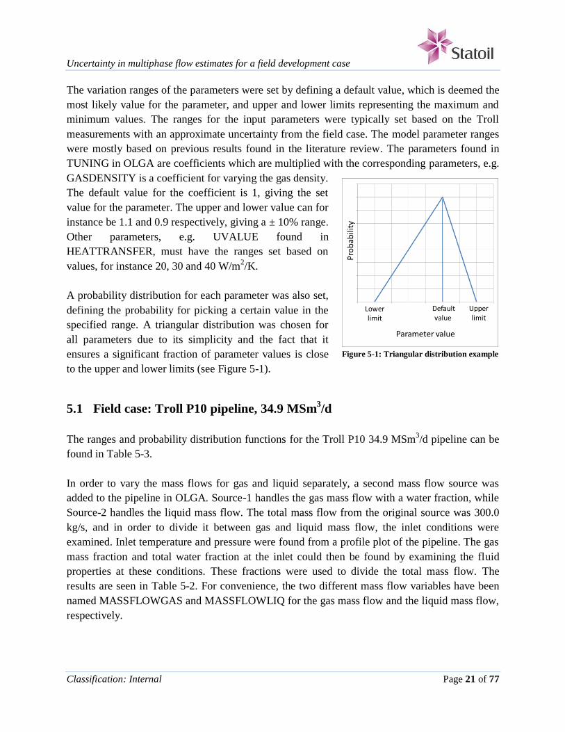
A probability distribution for each parameter was also set,
defining the probability for picking a certain value in the
specified range. A triangular distribution was chosen for
all parameters due to its simplicity and the fact that it
ensures a significant fraction of parameter values is close
to the upper and lower limits (see Figure 5-1).
5.1 Field case: Troll P10 pipeline, 34.9 MSm3/d
The ranges and probability distribution functions for the Troll P10 34.9 MSm3/d pipeline can be
found in Table 5-3.
In order to vary the mass flows for gas and liquid separately, a second mass flow source was
added to the pipeline in OLGA. Source-1 handles the gas mass flow with a water fraction, while
Source-2 handles the liquid mass flow. The total mass flow from the original source was 300.0
kg/s, and in order to divide it between gas and liquid mass flow, the inlet conditions were
examined. Inlet temperature and pressure were found from a profile plot of the pipeline. The gas
mass fraction and total water fraction at the inlet could then be found by examining the fluid
properties at these conditions. These fractions were used to divide the total mass flow. The
results are seen in Table 5-2. For convenience, the two different mass flow variables have been
named MASSFLOWGAS and MASSFLOWLIQ for the gas mass flow and the liquid mass flow,
respectively.
Figure 5-1: Triangular distribution example

Uncertainty in multiphase flow estimates for a field development case
Classification: Internal Page 22 of 77
Table 5-2: Inlet conditions for the P10 pipeline, 34.9 MSm3/d
Value at inlet Unit
Pressure 107.9 [bara]
Fluid temperature 44.5 [°C]
Gas mass fraction in gas/oil mixture 0.991 [-]
Total water fraction 0.00462 [-]
Gas mass flow 297.28 [kg/s]
Liquid mass flow 2.72 [kg/s]
Table 5-3: Ranges and distribution functions for input- and model parameters to be tested for the P10 pipeline, 34.9
MSm3/d
Parameter Lower
limit
Default
value
Upper
limit
Distribution
function
ANGLEDIAMPOWER 0 0 1.5 Triangular
ANGLESCALE 0 1 3 Triangular
DIAMPOWER 0.5 1 1.5 Triangular
ENTRAINMENT 0.1 1 3 Triangular
GASDENSITY 0.9 1 1.1 Triangular
GASVISC 0.9 1 1.1 Triangular
GROUGHNESS 0.5 1 6 Triangular
KTAHIGTFAC 0.7 1 1.3 Triangular
KTALOWTFAC 0.7 1 1.3 Triangular
KTGGRAVFAC 0.1 1 2 Triangular
KTGSMTHFAC 0.7 1 1.3 Triangular
KTGWAVYFAC 0.3 1 2.5 Triangular
LAM_LGI 0.8 1 1.7 Triangular
LAM_WOI 0.5 1 2 Triangular
MASSFLOWGAS 291.4 297.3 303.2 Triangular
MASSFLOWLIQ 0 2.72 5.44 Triangular
OILDENSITY 0.9 1 1.1 Triangular
OILVISC 0.7 1 1.3 Triangular
ROUGHNESS 0.5 1 2 Triangular
SIGGL 0.5 1 1.5 Triangular
TAMBIENT 0.5 1 1.3 Triangular
TOTALWATERFRACTION 0.00231 0.00462 0.00693 Triangular
UVALUE 20 30 40 Triangular
VOIDINSLUG 0.5 1 1.5 Triangular
VOIDINVERTSLUG 0.5 1 1.5 Triangular
WATERDENSITY 0.9 1 1.1 Triangular
WATERVISC 0.7 1 1.3 Triangular
WETFRACTION 0.7 1 1.3 Triangular

Uncertainty in multiphase flow estimates for a field development case
Classification: Internal Page 23 of 77
5.2 Field case: Troll P10 pipeline, 24.6 MSm3/d
The ranges and probability distribution functions for the Troll P10 24.6 MSm3/d pipeline can be
found in Table 5-5.
As for the friction dominated case, the mass flows for gas and liquid were varied separately by
adding a second mass flow source the pipeline in OLGA. The total mass flow from the original
source was 214.9 kg/s. In order to divide it between gas and liquid mass flow, the inlet
conditions were examined the same way as for the previous case. The results are seen in Table
5-4.
Table 5-4: Inlet conditions for the P10 pipeline, 24.6 MSm3/d
Value at inlet Unit
Pressure 102.8 [bara]
Fluid temperature 31.7 [°C]
Gas mass fraction in gas/oil mixture 0.983 [-]
Total water fraction 0.00564 [-]
Gas mass flow 211.2 [kg/s]
Liquid mass flow 3.65 [kg/s]
Table 5-5: Ranges and distribution functions for input- and model parameters to be tested for the P10 pipeline, 24.6
MSm3/d
Parameter Lower
limit
Default
value
Upper
limit
Distribution
function
ANGLEDIAMPOWER 0 0 1.5 Triangular
ANGLESCALE 0 1 3 Triangular
DIAMPOWER 0.5 1 1.5 Triangular
ENTRAINMENT 0.1 1 3 Triangular
GASDENSITY 0.9 1 1.1 Triangular
GASVISC 0.9 1 1.1 Triangular
GROUGHNESS 0.5 1 6 Triangular
KTAHIGTFAC 0.7 1 1.3 Triangular
KTALOWTFAC 0.7 1 1.3 Triangular
KTGGRAVFAC 0.1 1 2 Triangular
KTGSMTHFAC 0.7 1 1.3 Triangular
KTGWAVYFAC 0.3 1 2.5 Triangular
LAM_LGI 0.8 1 1.7 Triangular
LAM_WOI 0.5 1 2 Triangular
MASSFLOWGAS 206.9 211.2 215.4 Triangular
MASSFLOWLIQ 0 3.65 7.30 Triangular
OILDENSITY 0.9 1 1.1 Triangular
Uncertainty in multiphase flow estimates for a field development case
Classification: Internal Page 24 of 77
Parameter Lower
limit
Default
value
Upper
limit
Distribution
function
OILVISC 0.7 1 1.3 Triangular
ROUGHNESS 0.5 1 2 Triangular
SIGGL 0.5 1 1.5 Triangular
TAMBIENT 0.5 1 1.3 Triangular
TOTALWATERFRACTION 0.00282 0.00564 0.00846 Triangular
UVALUE 20 30 40 Triangular
VOIDINSLUG 0.5 1 1.5 Triangular
VOIDINVERTSLUG 0.5 1 1.5 Triangular
WATERDENSITY 0.9 1 1.1 Triangular
WATERVISC 0.7 1 1.3 Triangular
WETFRACTION 0.7 1 1.3 Triangular
Uncertainty in multiphase flow estimates for a field development case
Classification: Internal Page 25 of 77
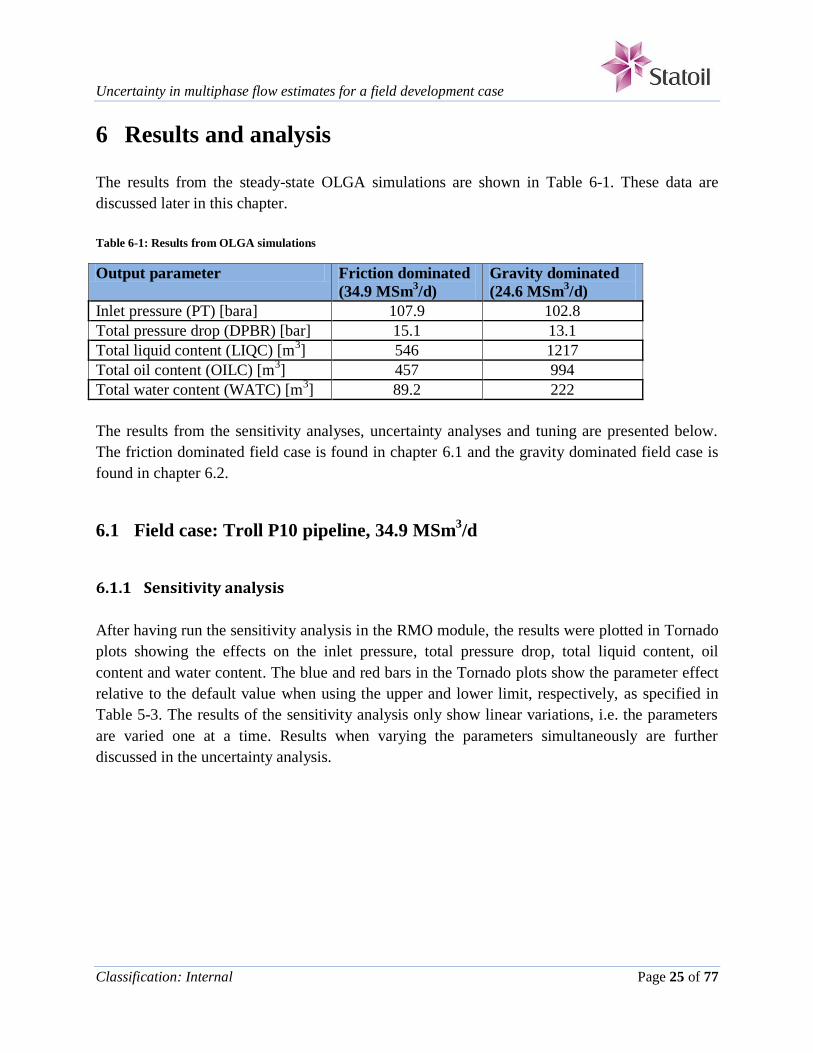
6 Results and analysis
The results from the steady-state OLGA simulations are shown in Table 6-1. These data are
discussed later in this chapter.
Table 6-1: Results from OLGA simulations
Output parameter Friction dominated
(34.9 MSm3/d)
Gravity dominated
(24.6 MSm3/d)
Inlet pressure (PT) [bara] 107.9 102.8
Total pressure drop (DPBR) [bar] 15.1 13.1
Total liquid content (LIQC) [m3] 546 1217
Total oil content (OILC) [m3] 457 994
Total water content (WATC) [m3] 89.2 222
The results from the sensitivity analyses, uncertainty analyses and tuning are presented below.
The friction dominated field case is found in chapter 6.1 and the gravity dominated field case is
found in chapter 6.2.
6.1 Field case: Troll P10 pipeline, 34.9 MSm3/d
6.1.1 Sensitivity analysis
After having run the sensitivity analysis in the RMO module, the results were plotted in Tornado
plots showing the effects on the inlet pressure, total pressure drop, total liquid content, oil
content and water content. The blue and red bars in the Tornado plots show the parameter effect
relative to the default value when using the upper and lower limit, respectively, as specified in
Table 5-3. The results of the sensitivity analysis only show linear variations, i.e. the parameters
are varied one at a time. Results when varying the parameters simultaneously are further
discussed in the uncertainty analysis.
Uncertainty in multiphase flow estimates for a field development case
Classification: Internal Page 26 of 77
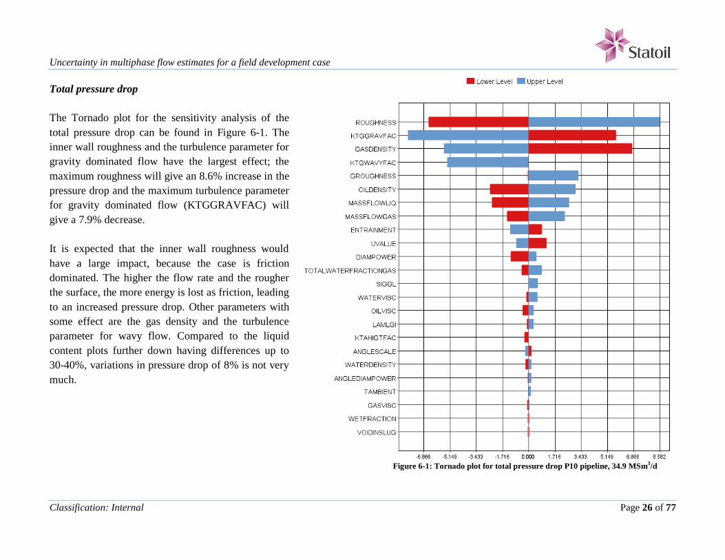
Total pressure drop
The Tornado plot for the sensitivity analysis of the
total pressure drop can be found in Figure 6-1. The
inner wall roughness and the turbulence parameter for
gravity dominated flow have the largest effect; the
maximum roughness will give an 8.6% increase in the
pressure drop and the maximum turbulence parameter
for gravity dominated flow (KTGGRAVFAC) will
give a 7.9% decrease.
It is expected that the inner wall roughness would
have a large impact, because the case is friction
dominated. The higher the flow rate and the rougher
the surface, the more energy is lost as friction, leading
to an increased pressure drop. Other parameters with
some effect are the gas density and the turbulence
parameter for wavy flow. Compared to the liquid
content plots further down having differences up to
30-40%, variations in pressure drop of 8% is not very
much.
Figure 6-1: Tornado plot for total pressure drop P10 pipeline, 34.9 MSm3/d

Uncertainty in multiphase flow estimates for a field development case
Classification: Internal Page 27 of 77
Inlet pressure
The Tornado plot for the sensitivity analysis of the inlet
pressure can be found in Figure 6-2. The most influential
parameters affecting the inlet pressure are the same as for
the total pressure drop: inner wall roughness, turbulence
parameters for gravity dominated flow and wavy flow,
and gas density. The change in pressure drop varies from
-1% to 1.2%.
Figure 6-2: Tornado plot for pressure at inlet P10 pipeline, 34.9 MSm3/d

Uncertainty in multiphase flow estimates for a field development case
Classification: Internal Page 28 of 77
Total liquid content
The Tornado plot for the sensitivity analysis of the total
liquid content can be found in Figure 6-3. The most
influential parameter for the total liquid content is the
liquid mass flow, giving a change of -27.9% to 28.9%
for the lower and upper limit, respectively. The high
impact of the liquid mass flow is expected, as increased
mass flow gives an increased liquid content.
Other important parameters are the turbulence
parameters for wavy flow and gravity dominated flow,
gas density, and ambient temperature. The liquid content
is decreasing with increasing turbulence parameters
since the interfacial friction increases, making the liquid
transport more efficient.
Figure 6-3: Tornado plot for total liquid content P10 pipeline, 34.9 MSm3/d
Uncertainty in multiphase flow estimates for a field development case
Classification: Internal Page 29 of 77
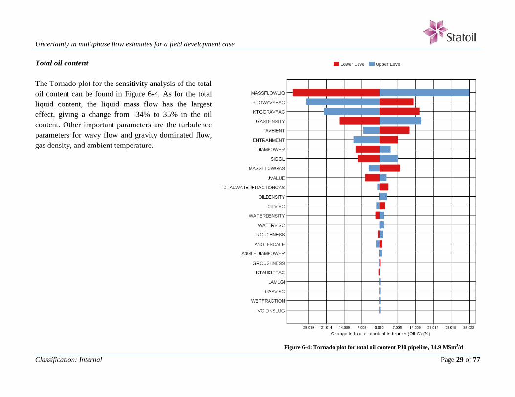
Total oil content
The Tornado plot for the sensitivity analysis of the total
oil content can be found in Figure 6-4. As for the total
liquid content, the liquid mass flow has the largest
effect, giving a change from -34% to 35% in the oil
content. Other important parameters are the turbulence
parameters for wavy flow and gravity dominated flow,
gas density, and ambient temperature.
Figure 6-4: Tornado plot for total oil content P10 pipeline, 34.9 MSm3/d

Uncertainty in multiphase flow estimates for a field development case
Classification: Internal Page 30 of 77
Total water content
The Tornado plot for the sensitivity analysis of the total
water content can be found in Figure 6-5. The total
water fraction has a significant impact on the water
content compared to the other parameters, giving a
change from -46% to 44%. This is expected, as the total
water fraction decides how much water is present in the
pipeline. The turbulence parameter for wavy flow and
the gas density also have a significant effect.
Figure 6-5: Tornado plot for total water content P10 pipeline, 34.9 MSm3/d

Uncertainty in multiphase flow estimates for a field development case
Classification: Internal Page 31 of 77
Summary
The most influential input- and model parameters are summarized in Table 6-2. The most
influential parameters are naturally the same for the inlet pressure and the pressure drop. Other
parameters which are influential for most output parameters are the mass flows of liquid and gas,
gas density, heat transfer coefficient, entrainment rate of droplets, and the turbulence parameters
for wavy flow and gravity dominated flow.
Table 6-2: Summary of results from sensitivity analysis, 34.9 MSm3/d
Output parameter Input parameters with the
largest effect
Model parameters
with the largest effect
PT
ROUGHNESS
GASDENSITY
OILDENSITY
MASSFLOWLIQ
MASSFLOWGAS
UVALUE
KTGGRAVFAC
KTGWAVYFAC
GROUGHNESS
ENTRAINMENT DPBR
LIQC MASSFLOWLIQ
GASDENSITY
TAMBIENT
SIGGL
TOTALWATERFRACTION
MASSFLOWGAS
UVALUE
KTGWAVYFAC
KTGGRAVFAC
ENTRAINMENT
DIAMPOWER
OILC MASSFLOWLIQ
GASDENSITY
TAMBIENT
SIGGL
MASSFLOWGAS
UVALUE
KTGWAVYFAC
KTGGRAVFAC
ENTRAINMENT
DIAMPOWER
WATC TOTALWATERFRACTION
GASDENSITY
WATERDENSITY
TAMBIENT
KTGWAVYFAC
KTGGRAVFAC

Uncertainty in multiphase flow estimates for a field development case
Classification: Internal Page 32 of 77
Parameters that do not appear at all in any of the Tornado plots i.e. have zero or near zero
contribution are:
KTGSMTHFAC: This is probably because the smooth turbulence parameter is only
applicable for very low gas Reynolds numbers, mostly laboratory conditions.
KTALOWTFAC: Similarly, this parameter is only applicable in cases of low turbulence
flow, which is not the case in the P10 pipeline.
VOIDINVERTSLUG and VOIDINSLUG: This indicates that there is no slug flow
present in the pipeline. This is verified by a profile plot of the flow regime indicator in
OLGA.
WETFRACTION
GASVISC
LAM_WOI
6.1.2 Uncertainty analysis
The results from the uncertainty analysis were shown using plots showing the distribution of the
inlet pressure, pressure drop, liquid content, oil content and water content when varying the
input- and model parameters. The blue columns represent the density distribution, the three red
columns show where the percentiles P10, P50 and P90 are located, and the light red columns
connected with a red line show the cumulative distribution.
Scatter plots of the data can be found in Appendix A.
Uncertainty in multiphase flow estimates for a field development case
Classification: Internal Page 33 of 77
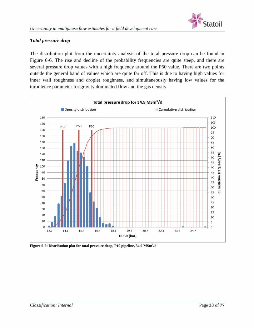
Total pressure drop
The distribution plot from the uncertainty analysis of the total pressure drop can be found in
Figure 6-6. The rise and decline of the probability frequencies are quite steep, and there are
several pressure drop values with a high frequency around the P50 value. There are two points
outside the general band of values which are quite far off. This is due to having high values for
inner wall roughness and droplet roughness, and simultaneously having low values for the
turbulence parameter for gravity dominated flow and the gas density.
Figure 6-6: Distribution plot for total pressure drop, P10 pipeline, 34.9 MSm3/d
Uncertainty in multiphase flow estimates for a field development case
Classification: Internal Page 34 of 77
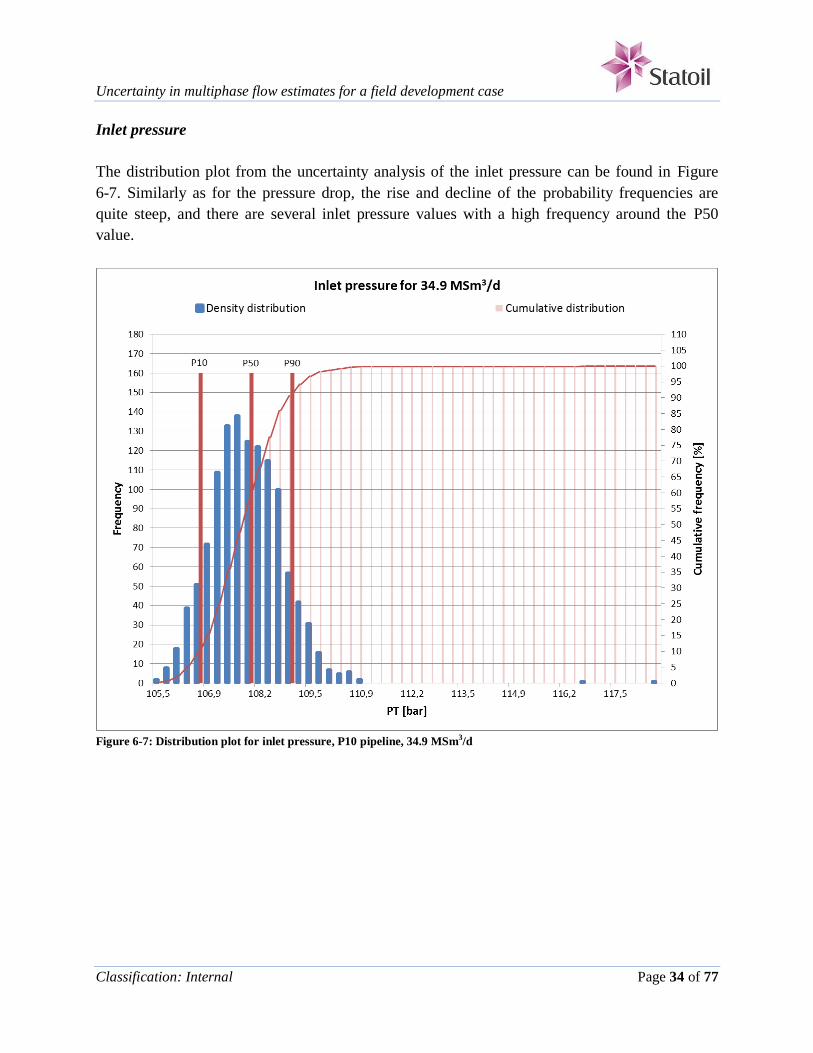
Inlet pressure
The distribution plot from the uncertainty analysis of the inlet pressure can be found in Figure
6-7. Similarly as for the pressure drop, the rise and decline of the probability frequencies are
quite steep, and there are several inlet pressure values with a high frequency around the P50
value.
Figure 6-7: Distribution plot for inlet pressure, P10 pipeline, 34.9 MSm3/d

Uncertainty in multiphase flow estimates for a field development case
Classification: Internal Page 35 of 77
Total liquid content
The distribution plot from the uncertainty analysis of the total liquid content can be found in
Figure 6-8. Here, the distribution is much wider compared to the pressure drop probability
distribution. This results in a more gradual slope of the cumulative distribution. There are more
points for the higher liquid content values, having low frequencies. Two points are quite far
away from the others, due to low values for the turbulence parameters for gravity dominated
flow and wavy flow, and the ambient temperature. For a wet gas such as the Troll gas, the
uncertainty in the liquid content is much higher than for the pressure drop.
Figure 6-8: Distribution plot for total liquid content, P10 pipeline, 34.9 MSm3/d
Uncertainty in multiphase flow estimates for a field development case
Classification: Internal Page 36 of 77
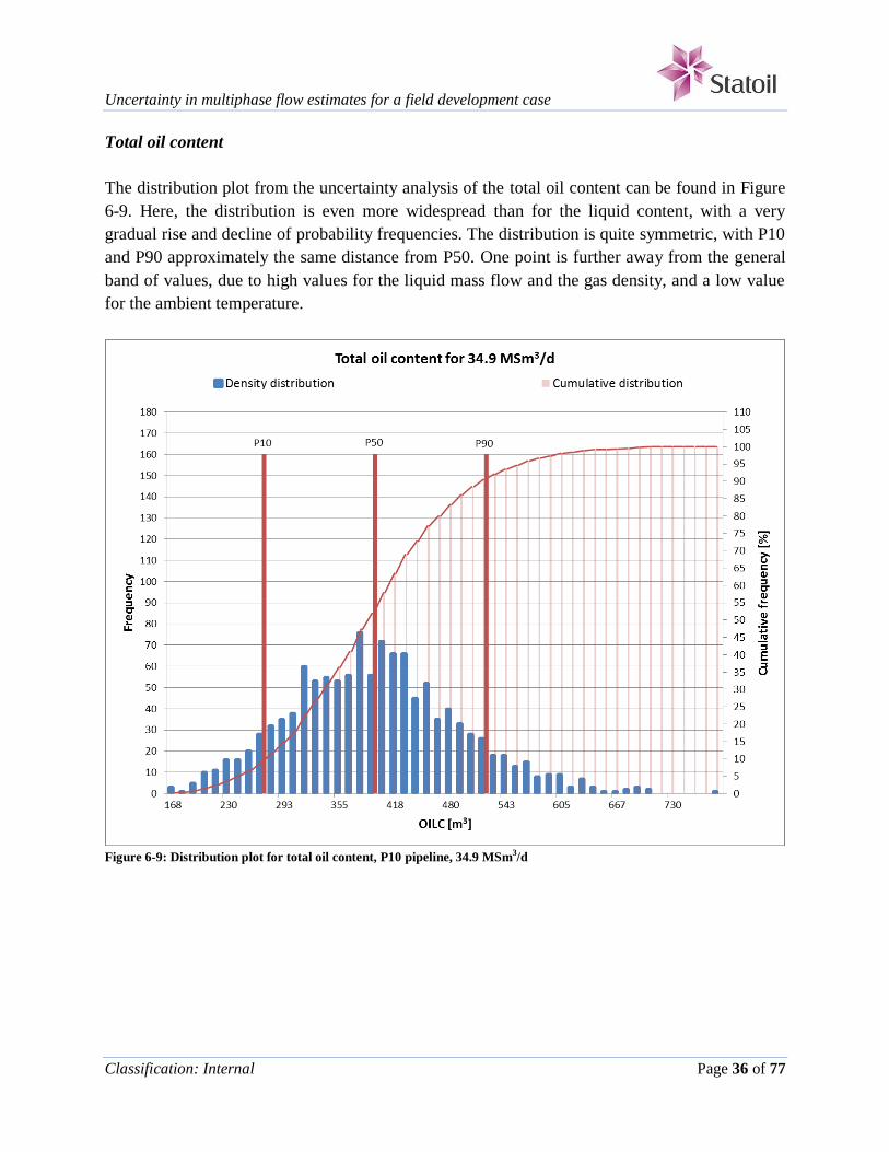
Total oil content
The distribution plot from the uncertainty analysis of the total oil content can be found in Figure
6-9. Here, the distribution is even more widespread than for the liquid content, with a very
gradual rise and decline of probability frequencies. The distribution is quite symmetric, with P10
and P90 approximately the same distance from P50. One point is further away from the general
band of values, due to high values for the liquid mass flow and the gas density, and a low value
for the ambient temperature.
Figure 6-9: Distribution plot for total oil content, P10 pipeline, 34.9 MSm3/d

Uncertainty in multiphase flow estimates for a field development case
Classification: Internal Page 37 of 77
Total water content
The distribution plot from the uncertainty analysis of the total water content can be found in
Figure 6-10. The distribution is quite narrow with high probability frequencies for the lower
water content values, followed by a tail of values with very low frequencies. There are also two
extreme values far away from the others. This is due to a somewhat high total water fraction, and
low values for the turbulence parameter for gravity dominated flow and ambient temperature.
Figure 6-10: Distribution plot for total water content, P10 pipeline, 34.9 MSm3/d

Uncertainty in multiphase flow estimates for a field development case
Classification: Internal Page 38 of 77
Summary
In Table 6-3 is a summary of the key data in the distribution plots. The minimum and maximum
values for the output parameters are the minimum and maximum values of the general band
containing the output values, i.e. none of the extreme values. The default value is the one value
OLGA calculates for the output parameter. Two different kinds of uncertainties are also stated;
one showing the difference between P10 and P50 (-), and between P50 and P90 (+), and the
other showing the difference between the minimum and default value (-), and the default and
maximum value (+). A comparison of these results with the measurement data from the Troll
P10 pipeline can be found in Table 6-4.
Table 6-3: Summary of results from uncertainty analysis, 34.9 MSm3/d
Output
variable
P10 P50 P90 Min. Default Max. Uncertainty
P10-P50-P90
Uncertainty
Min-Default-Max
PT
[bar] 106.8 107.9 109.1 105.4 107.9 111.0 -1.0% / +1.1% -2.3% / +2.9%
DPBR
[bar] 14.0 15.1 16.3 12.6 15.1 18.2 -7.4% / +8.0% -16.5% / +20.5%
LIQC
[m3]
359 479 624 240 546 891 -25.1% / +30.3% -56.0% / +63.2%
OILC
[m3]
278 394 521 162 457 786 -29.4% / +32.3% -64.6% / +72.1%
WATC
[m3]
64.1 86.7 108 48.0 89.2 278 -26.1% / +24.4% -46.2% / +212%
The uncertainties for the liquid, oil and water content are quite high compared to the inlet
pressure and pressure drop. When comparing the two different uncertainties, the Min-Default-
Max uncertainty is significantly larger than the P10-P50-P90 uncertainty for most cases. This
shows that some calculations can be quite high or low, even though they do not occur as
frequent.

Uncertainty in multiphase flow estimates for a field development case
Classification: Internal Page 39 of 77
Table 6-4: Comparison with Troll measurement data, 34.9 MSm3/d
Troll
measurement
OLGA
calculation
Within
P10-P90
Within
Min-Max
P- value the
measurement
represents
Inlet pressure [bara] 105.5 107.9 No Yes P0.3
Pressure drop [bar] 12.7 15.1 No Yes P0.3
Total liquid
accumulation [m3]
279 546 No Yes P1.2
Condensate
accumulation [m3]
165 457 No Yes P0.1
Water accumulation
[m3]
114 89.2 No Yes P94
From this it is seen that none of the measurements fall inside the P10-P90 uncertainty range, and
all are barely within the Min-Max range. For all output parameters except the water content, the
measurement value is just above the minimum value, indicating that OLGA tends to over-predict
the output parameters.
6.1.3 Tuning
For this friction dominated case, there was an over-prediction of the output parameters compared
to the field measurements, with the exception of the water content. However, the under-
prediction of the water content is a known weakness of the OLGA HD 7.1.4 model (Nygård,
2012) (Valle & Johansson, 2011). This is supposed to be improved in OLGA 7.2.0., and because
the water content prediction is so uncertain, it was not worthwhile to take it into account. Thus, it
was of interest to tune some of the most influential model parameters to shift the OLGA
predictions towards lower values in order to get closer to the measurements. As of today, there
are few model parameters available for tuning the oil-water interfacial friction in OLGA. It was
therefore necessary to accept what was available. As seen in the sensitivity analysis, two model
parameters which were quite influential on all the output parameters were KTGGRAVFAC and
KTGWAVYFAC. A higher value for these gave a lower value for the pressure drop and liquid
content. Consequently, a new uncertainty analysis with a shifted range (Table 6-5) for these
model parameters was performed, while all other parameter ranges were set as before.
Table 6-5: Tuned parameters, 34.9 MSm3/d
Model parameter Lower
limit
Default
value
Upper
limit
KTGGRAVFAC 1 2 3
KTGWAVYFAC 1 2 3

Uncertainty in multiphase flow estimates for a field development case
Classification: Internal Page 40 of 77
The results from the tuning are summarized in Table 6-6. A comparison with Troll data is shown
in Table 6-7. Scatter plots and distribution plots can be found in Appendix B.
Table 6-6: Summary of results from tuning, 34.9 MSm3/d
Output
variable
P10 P50 P90 Min. Default Max. Uncertainty
P10-P50-P90
Uncertainty
Min-Default-Max
PT
[bar] 106.2 107.2 108.2 104.9 106.9 110.1 -0.9% / +0.9% -1.9% / +3.0%
DPBR
[bar] 13.4 14.4 15.4 12.1 14.1 17.3 -7.0% / +6.7% -14.2% / +22.9%
LIQC
[m3]
309 385 471 224 394 592 -20.0% / +22.4% -43.0% / +50.2%
OILC
[m3]
226 306 394 154 314 506 -26.2% / +28.6% -50.9% / +60.9%
WATC
[m3]
61.1 80.4 102 44.3 79.9 126 -23.9% / +26.4% -44.5% / +58%
Compared to the uncertainty analysis, all the tuned results are lower in value. Especially for the
liquid content, the P90 and maximum values are significantly reduced. The P10-P50-P90
uncertainties are generally smaller for the tuned values. The Min-Default uncertainties (-) are
slightly smaller and the Default-Max uncertainties (+) are slightly larger for the inlet pressure
and pressure drop. For the liquid and oil content the Min-Default-Max uncertainties are
significantly smaller.
Table 6-7: Comparison of tuning with Troll measurement data, 34.9 MSm3/d
Troll
measurement
OLGA
calculation
Within
P10-P90
Within
Min-Max
P- value the
measurement
represents
Inlet pressure [bara] 105.5 106.9 No Yes P1
Pressure drop [bar] 12.7 14.1 No Yes P1
Total liquid
accumulation [m3]
279 394 No Yes P4
Condensate
accumulation [m3]
165 314 No Yes P0.4
Water accumulation
[m3]
114 79.9 No Yes P99
The OLGA predictions are closer to the Troll measurements after the tuning, but they are still
higher than the measured values. The percentile values the measurement values represent in the
OLGA output distributions are higher than before the tuning. However, they are still very low in
value, meaning that the measurements are close to the minimum values obtained from the

Uncertainty in multiphase flow estimates for a field development case
Classification: Internal Page 41 of 77
analysis. The exception again is the water content which is under-predicted, with a percentile
value close to the maximum. All the measurements are still within the minimum and maximum
values, but none are within P10 and P90.
6.2 Field case: Troll P10 pipeline, 24.6 MSm3/d
6.2.1 Sensitivity analysis
After having run the sensitivity analysis in the RMO module, the results were plotted in Tornado
plots showing the effects on the inlet pressure, total pressure drop, total liquid content, oil
content and water content. The blue and red bars in the Tornado plots show the parameter effect
relative to the default value when using the upper and lower limit, respectively, as specified in
Table 5-5. The results of the sensitivity analysis only show linear variations, i.e. the parameters
are varied one at a time. Results when varying the parameters simultaneously are further
discussed in the uncertainty analysis.

Uncertainty in multiphase flow estimates for a field development case
Classification: Internal Page 42 of 77
Total pressure drop
The Tornado plot for the sensitivity analysis of the
total pressure drop can be found in Figure 6-11. The
most influential parameter is the turbulence parameter
for gravity dominated flow, giving a range in pressure
drop from -21% to 11%. This parameter has a large
effect because the flow is gravity dominated and many
of the pipe sections have high liquid holdup values.
Other parameters with some effect are the oil density,
the turbulence parameter for wavy flow, void in slug
and the inner wall roughness. The fact that the void in
slug parameter appears in the list shows that OLGA
predicts slug flow in the high inclined sections towards
the landfall.
Figure 6-11: Tornado plot for total pressure drop P10 pipeline, 24.6 MSm3/d

Uncertainty in multiphase flow estimates for a field development case
Classification: Internal Page 43 of 77
Inlet pressure
The Tornado plot for the sensitivity analysis of the inlet
pressure can be found in Figure 6-12. The most
influential parameters affecting the inlet pressure are the
same as for the pressure drop: the turbulence parameters
for gravity dominated flow and wavy flow, oil density,
void in slug and the inner wall roughness. The range in
inlet pressure is from -2.7% to 1.4%. Compared to the
liquid content plots further down having much larger
differences, variations in inlet pressure of 2% is not
very much. However, in relation to the pressure drop,
2% change at the inlet is more significant.
Figure 6-12: Tornado plot for pressure at inlet P10 pipeline, 24.6 MSm3/d

Uncertainty in multiphase flow estimates for a field development case
Classification: Internal Page 44 of 77
Total liquid content
The Tornado plot for the sensitivity analysis of the
total liquid content can be found in Figure 6-13. The
most influential parameters are the turbulence
parameters for gravity dominated flow and wavy flow,
and the liquid mass flow. The variation in liquid
content is from -29% to 22%. Other significant
parameters are the gas density, void in slug and the
total water fraction.
Figure 6-13: Tornado plot for total liquid content P10 pipeline, 24.6 MSm3/d

Uncertainty in multiphase flow estimates for a field development case
Classification: Internal Page 45 of 77
Total oil content
The Tornado plot for the sensitivity analysis of the
total oil content can be found in Figure 6-14. The
most influential parameter is the liquid mass flow,
giving a range in oil content from -36% to 30%.
Other significant parameters are the turbulence
parameters for gravity dominated flow and wavy
flow, void in slug, oil and gas densities and the
tuning coefficient for interfacial friction factor
(liquid-gas).
Figure 6-14: Tornado plot for total oil content P10 pipeline, 24.6 MSm3/d

Uncertainty in multiphase flow estimates for a field development case
Classification: Internal Page 46 of 77
Total water content
The Tornado plot for the sensitivity analysis of the
total water content can be found in Figure 6-15. The
most influential parameter is the turbulence
parameter for gravity dominated flow giving a range
of the water content from -40% to 124%. Other
significant parameters are the oil and gas densities,
the total water fraction, the liquid mass flow, void in
slug, and the tuning coefficients for interfacial
friction factors for gas/liquid and oil/water in the
slug model (LAMLGI and LAMWOI).
Figure 6-15: Tornado plot for total water content P10 pipeline, 24.6 MSm3/d

Uncertainty in multiphase flow estimates for a field development case
Classification: Internal Page 47 of 77
Summary
The most influential input- and model parameters are summarized in Table 6-8. The most
influential parameters are naturally the same for the inlet pressure and the pressure drop. Other
parameters which are influential for most output parameters are the mass flows of liquid and gas,
oil and gas densities, total water fraction, the tuning coefficient for void in slug, and the
turbulence parameters for wavy flow and gravity dominated flow.
Table 6-8: Summary of results from sensitivity analysis, 24.6 MSm3/d
Output parameter Input parameters with the
largest effect
Model parameters with the
largest effect
PT OILDENSITY
TOTALWATERFRACTION
MASSFLOWLIQ
ROUGHNESS
GASDENSITY
KTGGRAVFAC
KTGWAVYFAC
VOIDINSLUG
LAM_WOI DPBR
LIQC MASSFLOWLIQ
GASDENSITY
TOTALWATERFRACTION
SIGGL
TAMBIENT
MASSFLOWGAS
OILDENSITY
KTGGRAVFAC
KTGWAVYFAC
VOIDINSLUG
OILC MASSFLOWLIQ
OILDENSITY
GASDENSITY
TOTALWATERFRACTION
SIGGL
TAMBIENT
KTGGRAVFAC
LAM_LGI
KTGWAVYFAC
VOIDINSLUG
LAM_WOI
WATC TOTALWATERFRACTION
OILDENSITY
GASDENSITY
MASSFLOWLIQ
MASSFLOWGAS
KTGGRAVFAC
LAM_LGI
VOIDINSLUG
LAM_WOI
KTGWAVYFAC

Uncertainty in multiphase flow estimates for a field development case
Classification: Internal Page 48 of 77
Parameters that do not appear at all in any of the Tornado plots i.e. have zero or near zero
contribution are:
KTGSMTHFAC: This is probably because the smooth turbulence parameter is only
applicable for very low gas Reynolds numbers, mostly laboratory conditions
KTALOWTFAC: Similarly, this parameter is only applicable in cases of low turbulence
flow, which is not the case in the P10 pipeline.
KTAHIGHTFAC
WETFRACTION
GASVISC
ANGLESCALE
ANGLEDIAMPOWER
6.2.2 Uncertainty analysis
The results from the uncertainty analysis were shown using plots showing the distribution of the
inlet pressure, pressure drop, liquid content, oil content and water content when varying the
input- and model parameters. The blue columns represent the density distribution, the three red
columns show where the percentiles P10, P50 and P90 are located, and the light red columns
connected with a red line show the cumulative distribution.
Scatter plots of the data can be found in Appendix A.

Uncertainty in multiphase flow estimates for a field development case
Classification: Internal Page 49 of 77
Total pressure drop
The distribution plot from the uncertainty analysis of the total pressure drop can be found in
Figure 6-16. The distribution rises and declines gradually and there are several points beyond
P90 with low probability frequencies, making the distribution slightly skewed.
Figure 6-16: Distribution plot for total pressure drop, P10 pipeline, 24.6 MSm
3/d
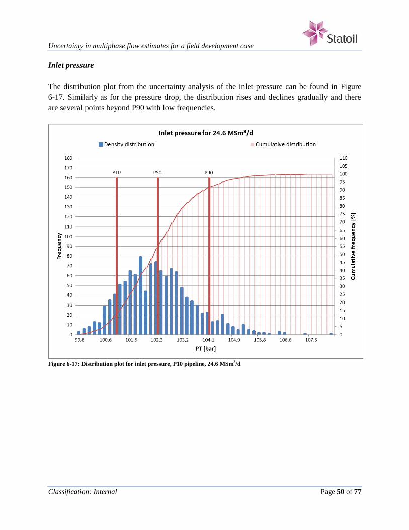
Uncertainty in multiphase flow estimates for a field development case
Classification: Internal Page 50 of 77
Inlet pressure
The distribution plot from the uncertainty analysis of the inlet pressure can be found in Figure
6-17. Similarly as for the pressure drop, the distribution rises and declines gradually and there
are several points beyond P90 with low frequencies.
Figure 6-17: Distribution plot for inlet pressure, P10 pipeline, 24.6 MSm3/d

Uncertainty in multiphase flow estimates for a field development case
Classification: Internal Page 51 of 77
Total liquid content
The distribution plot from the uncertainty analysis of the total liquid content can be found in
Figure 6-18. The probability distribution is rather flat and widespread. There is a band of values
near P50 which have similar probability frequencies.
Figure 6-18: Distribution plot for total liquid content, P10 pipeline, 24.6 MSm
3/d

Uncertainty in multiphase flow estimates for a field development case
Classification: Internal Page 52 of 77
Total oil content
The distribution plot from the uncertainty analysis of the total oil content can be found in Figure
6-19. The distribution is quite widespread and gradual. There is a band of values near P50 which
have similar probability frequencies; there is no definite peak. There are some high values with
low frequencies, resulting in P90 being further away from P50.
Figure 6-19: Distribution plot for total oil content, P10 pipeline, 24.6 MSm3/d

Uncertainty in multiphase flow estimates for a field development case
Classification: Internal Page 53 of 77
Total water content
The distribution plot from the uncertainty analysis of the total water content can be found in
Figure 6-20. The distribution is quite skewed, with a steep rise towards P50 and a very gradual
decline after. Most of the higher values have very low probability frequencies, but there are
many of them, so P90 is shifted to the right.
Figure 6-20: Distribution plot for total water content, pipeline, 24.6 MSm3/d

Uncertainty in multiphase flow estimates for a field development case
Classification: Internal Page 54 of 77
Summary
In Table 6-9 is a summary of the key data in the distribution plots. The minimum and maximum
values for the output parameters are the minimum and maximum values of the general band
containing the output values, i.e. none of the extreme values. The default value is the one value
OLGA calculates for the output parameter. Two different kinds of uncertainties are also stated;
one showing the difference between P10 and P50 (-), and between P50 and P90 (+), and the
other showing the difference between the minimum and default value (-), and the default and
maximum value (+). A comparison of these results with the measurement data from the Troll
P10 pipeline can be found in Table 6-10.
Table 6-9: Summary of results from uncertainty analysis, 24.6 MSm3/d
Output
variable
P10 P50 P90 Min. Default Max. Uncertainty
P10-P50-P90
Uncertainty
Min-Default-Max
PT
[bar] 100.9 102.3 104.0 99.7 102.8 111.0 -1.3% / +1.7% -3.0% / +8.0%
DPBR
[bar] 11.3 12.6 14.3 10.0 13.1 18.6 -10.8% / +13.4% -23.7% / +41.8%
LIQC
[m3]
872 1110 1346 591 1217 1747 -21.5% / +21.2% -51.4% / +43.6%
OILC
[m3]
661 896 1118 387 994 1534 -26.3% / +24.8% -61.1% / +54.2%
WATC
[m3]
115 176 380 73.3 222 947 -34.6% / +116% -67.0% / +326%
For the inlet pressure and the pressure drop the OLGA calculations are quite close to the P50
values, while for the liquid, oil and water content the calculations are higher. The uncertainties
for liquid, oil and water content are generally very high. When comparing the two different
uncertainties, the Min-Default-Max uncertainty is significantly larger than the P10-P50-P90
uncertainty, especially for the water content. This shows that some calculations can be quite high
or low, even though they do not occur as frequent.

Uncertainty in multiphase flow estimates for a field development case
Classification: Internal Page 55 of 77
Table 6-10: Comparison with Troll measurement data, 24.6 MSm3/d
Troll
measurement
OLGA
calculation
Within
P10-P90
Within
Min-Max
P- value the
measurement
represents
Inlet pressure [bara] 101.7 102.8 Yes Yes P30
Pressure drop [bar] 12.0 13.1 Yes Yes P30
Total liquid
accumulation [m3]
1386 1217 No Yes P100
Condensate
accumulation [m3]
856 994 Yes Yes P42
Water accumulation
[m3]
530 222 No Yes P97
From this it is seen that the inlet pressure, pressure drop and oil content measurements fall inside
the P10-P90 uncertainty range and all measurements are within the Min-Max range. For this
gravity dominated case the measured liquid accumulation is much higher than for the friction
dominated case and OLGA under-predicts it. Thus, the measured liquid content represents a high
percentile value. The water content is just within the maximum value. The measured inlet
pressure, pressure drop and oil content are between the P10 and P50 value.
6.2.3 Tuning
For this gravity dominated case, there was generally an over-prediction of the pressure drop
compared to the field measurements. The liquid content and water content are, however, under-
predicted which is different from the friction dominated case. In addition, the uncertainties for
the gravity dominated case are much larger. This makes a general tuning difficult. By trying to
achieve higher values for the calculations, the liquid content will be even more over-predicted.
Due to OLGA 7.1.4’s poor calculation of water content (Nygård, 2012) (Valle & Johansson,
2011), the water accumulation has not been taken into account. Therefore it was decided to
perform the same tuning as for the friction dominated case, to get a background for comparison.
A new uncertainty analysis with a shifted range for KTGGRAVFAC and KTGWAVYFAC was
executed (Table 6-5), while all other parameter ranges were the same as before. The results are
summarized in Table 6-11, and a comparison with Troll measurements is found in Table 6-12.
Scatter plots and distribution plots can be found in Appendix B.

Uncertainty in multiphase flow estimates for a field development case
Classification: Internal Page 56 of 77
Table 6-11: Summary of results from tuning, 24.6 MSm3/d
Output
variable
P10 P50 P90 Min. Default Max. Uncertainty
P10-P50-P90
Uncertainty
Min-Default-Max
PT
[bar] 99.2 100.3 101.8 98.0 100.1 103.8 -1.1% / +1.5% -2.1% / +3.7%
DPBR
[bar] 9.5 10.6 12.1 8.3 10.5 14.1 -10.4% / +14.0% -21.0% / +34.7%
LIQC
[m3]
631 834 1051 432 821 1388 -24.4% / +26.0% -47.4% / +69.1%
OILC
[m3]
502 704 912 303 695 1222 -28.7% / +29.7% -56.3% / +75.9%
WATC
[m3]
95.5 131 169 64.9 126 314 -26.9% / +29.6% -48.5% / +150%
Compared to the uncertainty analysis, all the output results from the tuned simulations are a great
deal lower in value, especially the maximum values. The P10-P50-P90 uncertainties are quite
similar as before for the tuned inlet pressure and pressure drop, while the Min-Default-Max
uncertainties are lower. For the liquid and oil content, the P10-P50-P90 uncertainties are higher
after the tuning, the Min-Default (-) uncertainties are smaller, and the Default-Max (+)
uncertainties are higher. For the water content, all uncertainties are lower for the tuned results.
Table 6-12: Comparison of tuning with Troll measurement data, 24.6 MSm3/d
Troll
measurement
OLGA
calculation
Within
P10-P90
Within
Min-Max
P- value the
measurement
represents
Inlet pressure [bara] 101.7 100.1 Yes Yes P89
Pressure drop [bar] 12.0 10.5 Yes Yes P89
Total liquid
accumulation [m3]
1386 821 No Yes P100
Condensate
accumulation [m3]
856 695 Yes Yes P82
Water accumulation
[m3]
530 126 No No Over P100
The OLGA calculations are not closer to the Troll measurements after the tuning; the tuned
values are now lower than the measurements. This is also seen in the percentile values of the
measurements, as they are now considerably higher than before. With the exception of the water
content, all the measurements are still within the minimum and maximum values, and the inlet
pressure, pressure drop and oil content are still within P10 and P90. The water content is now
very under-predicted, and the measurement is far above the maximum value obtained in the
tuning, i.e. over P100.
Uncertainty in multiphase flow estimates for a field development case
Classification: Internal Page 57 of 77
7 Discussion
7.1 On using the RMO module for uncertainty estimation
The module is easily accessed from OLGA, and it does not take long to set up analyses with
ranges and distributions. The features for the sensitivity analysis and the uncertainty analysis are
user friendly and not difficult to understand. The tuning/optimization cycle, however, was not
found to be very intuitive and was not used in this project. After setting up an analysis, the
simulations can be started and will then run by themselves automatically until completed, which
is very practical. The automatic Tornado plots generated from the sensitivity analyses are good,
although editing the design and appearance of the plot is quite time consuming and not very
intuitive. The visualization tools for the uncertainty analyses are useful; there are several
different plot options for the data and there is a user guide available for these in the RMO
module. It is also very easy to export the different data sets to e.g. Microsoft Excel if that is
preferred instead. The RMO module is a good alternative to using the full MEPO program if all
that is needed are the uncertainty estimation features.
The negative experience with the RMO module is that it often behaves erratically, and the user
does not have many options to fix the problems. The RMO analyses are opened automatically
when entering the module from OLGA, and if for some reason it cannot find the files there is no
way to open them manually. The backup files must then be accessed to see if a previous version
can be opened instead, potentially causing loss of data. The module also crashed several times
during the analyses for no apparent reason, and exited the module without warning. This also
causes loss of data, as the analyses must finish and then be saved in the program to be stored on
the computer. The uncertainty analysis may take hours or days to execute, and it is problematic if
the RMO module suddenly turns off during the simulations. The idea for executing the analyses
for this project was so set up simulations during the day, and let them run overnight and assess
the results the next day. Unfortunately, due to these shut downs, this proved difficult. Small
batches of simulations had to be performed under supervision instead, to ensure storage of the
results along the way. Thus, this proved a lot more time consuming than anticipated, and became
much more inconvenient.
More an annoyance than an actual problem is the fact that the program sometimes freezes, and
can spend a lot of time opening and closing, switching between analyses, and post-processing the
data. The RMO module also does not seem to handle alterations in the OLGA project, e.g. if the
OLGA project is run after an analysis has been performed in the RMO module, it will not be able
to run a new analysis because the OLGA project is changed. According to SPT Group, many of
Uncertainty in multiphase flow estimates for a field development case
Classification: Internal Page 58 of 77
these issues with the RMO module are resolved in OLGA 7.2. Until the new version is available,
further use of the RMO module is not recommended.
It would probably have been beneficial to have attended SPT Group’s course, or at least learned
the program from someone who knows it. This would have been especially useful for the tuning
function. Better understanding of all the functions could lead to improved use, which again could
lead to fewer errors. However, these courses are quite expensive, and there was no opportunity to
take such a course during this project.
7.2 On the results
The sensitivity analyses showed the linear effect of the minimum and maximum values of the
input- and model parameters on the output parameters. For the friction dominated case, input
parameters that had significant impact were densities of oil and gas, mass flows of liquid and
gas, inner wall roughness, heat transfer coefficient, surface tension liquid/gas and the ambient
temperature. Model parameters with a large effect were turbulence parameters for gravity
dominated flow and for wavy flow, droplet roughness, entrainment rate of droplets and the
diameter exponent in the droplet entrainment scaling expression. For the gravity dominated case,
significant input parameters were much the same as for the friction dominated case, with the
exception of the heat transfer coefficient. The total water fraction also had a larger effect for the
gravity dominated case. Important model parameters were turbulence parameters for gravity
dominated flow and for wavy flow, tuning coefficient for void in slug flow, and the interfacial
friction factors (liquid-gas and oil-water).
The mass flow rates, densities and surface tension were expected to be significant for both cases,
as these input parameters influence the flow regimes and thus the general behavior of the flow.
For the friction dominated case, the flow rates are higher, meaning that wall and droplet
roughness will have a large impact on the pressure drop. Droplet entrainment from liquid to the
gas is also important; a high entrainment rate will tear off droplets from the liquid layer, thus
resulting in a decreased liquid content and a decrease in hydrostatic pressure drop. These
parameters are also important for the gravity dominated case, although not to the same extent
because the flow rates are lower. For both cases, a low ambient temperature gives an increase in
liquid content, due to the fact that more liquid is condensed from the gas at low temperatures.
This is approximately the same effect as having a high heat transfer coefficient; the fluids in the
pipe will cool faster due to the colder sea temperature outside the pipe. The total water fraction is
more significant for the gravity dominated case, because there in more liquid in the pipe and
OLGA calculates more sections with high holdup solutions. A small addition of water can result
in a high holdup solution, giving a relatively high sensitivity of this parameter.

Uncertainty in multiphase flow estimates for a field development case
Classification: Internal Page 59 of 77
The turbulence parameters had a large impact in both cases. The turbulence parameter for wavy
flow was not surprising, as there is mostly wavy flow in the pipeline, but it was unexpected that
the turbulence parameter for gravity dominated flow would have such significance in the friction
dominated case. The expectation was that it would only impact the gravity dominated case. A
possible explanation could have been that OLGA calculates high holdup solutions somewhere in
the pipeline which causes it to have an effect, but after checking the output from OLGA it was
found that the friction dominated case does not have any sections with high holdup. It is,
however, possible that the KTGGRAVFAC parameter is important in the high inclination
sections towards the landfall (see Figure 3-3) even though the holdup is not larger than about 0.1.
The equations used in OLGA are confidential to SPT Group, thus making it difficult to
determine why this parameter influences the output so much. For the gravity dominated case,
there was also an effect from the tuning coefficient for void in slug, meaning there is transition to
slug flow in the high inclined sections towards the landfall. Different flow regimes cause the
flow to behave differently, so the parameter has a significant effect. The interfacial friction
factors were also important in this case; a high interfacial friction factor makes it easier for the
gas to drag the liquid along the pipeline, thus giving a decrease in required pressure drop. It was
also expected that high interfacial friction would also give a decrease in liquid content, but the
sensitivity analysis showed the opposite. An explanation was found when looking at the OLGA
output. At the end of the P10 pipeline, where it rises to shore, there are areas where OLGA
calculates transition to a slug flow regime. When increasing the friction factor, tendencies to slug
flow are reduced, giving wavy flow instead. Wavy flow has a higher liquid content than slug
flow, thus giving a larger value. Consequently, increased interfacial friction does not give a
higher liquid content; this is caused by the resulting flow regime transition. This shows the
complexity associated with parameter tuning and its effect on flow regime transitions.
For both cases, the changes in output values were higher for the liquid, oil and water content
compared to the pressure drop and inlet pressure. This means that the total liquid content is more
sensitive to changes in the input- and model parameters. When looking at the friction dominated
case compared to the gravity dominated case, the changes in the pressure drop are much larger
for the gravity dominated case. The changes in liquid and oil content are quite similar for the two
cases, while the water content has a very high upper value for the gravity dominated case.
Generally, the gravity dominated case was more sensitive to input- and model parameter
variations than the friction dominated case.
From the uncertainty analyses it was found that the linear effects from the sensitivity analyses
could amplify or cancel each other when varying the parameters simultaneously. For the friction
dominated case, the density distribution of the pressure drop was quite steep, with high
probability frequencies near the P50 value. The distributions for the liquid and oil contents were
more widespread with gradual rise and decline in probability frequencies. The water content
Uncertainty in multiphase flow estimates for a field development case
Classification: Internal Page 60 of 77
distribution was very narrow with many high frequencies, followed by a tail of higher values
with very low frequencies. For the gravity dominated case, the density distributions of the output
parameters were generally much more widespread than for the friction dominated case. The
water content density distribution was quite skewed, with higher frequencies for values between
P10 and P50, and then a very gradual decline towards and past P90.
When looking at the uncertainties of P10 and P90 with respect to P50, and the uncertainties of
the minimum and maximum values with respect to the default value, the uncertainties in the
friction dominated case are smaller for the inlet pressure, pressure drop and water content, and
larger for the total liquid content and the oil content, compared to the gravity dominated case.
However, the liquid content values for the gravity dominated case are generally much higher
than for the friction dominated case, and the difference between minimum and maximum values
are significantly larger. For both cases, the Min-Default-Max uncertainties are approximately the
double of the P10-P50-P90 uncertainties, showing that there are many high and low values
outside the P10-P90 span with small density frequencies. Especially for the water content, the
maximum value is very large. For both cases, uncertainties in the inlet pressure and pressure
drop are small compared to the liquid contents, indicating that the Troll pipeline pressure drop is
not as sensitive to the changes in the input- and model parameters.
For the friction dominated case, the measured Troll values approximately represented a
percentile P1, i.e. 99 % of the predicted values were higher than the measurements. The water
content was an exception, with a measurement representing P94. As stated previously, OLGA
7.1.4 does not predict water content adequately; consequently the water content will not be
discussed further. Thus, OLGA over-predicts the output parameters in the friction dominated
case. The gravity dominated case was quite different. The measured inlet pressure, pressure drop
and oil content were all inside the P10-P90 range, while the measured total liquid content and
water content were under-predicted as the measurements represented approximately P100. As
stated earlier, the under-prediction of water content is a known problem for OLGA 7.1.4, so this
is one reason why the total liquid content is under-predicted. Another reason is the fact that
OLGA predicts slug flow in the high inclined parts of the pipeline, giving a lower liquid
inventory. Turning off the slug model in OLGA improves the prediction of liquid accumulation
for the gravity dominated case. The uncertainty ranges in this case are quite large, and this may
be a reason why the measurements fall inside the output distribution.
The tuning sessions were performed to attempt to shift the OLGA calculations closer to the Troll
measurements. For the friction dominated case, this was straightforward to do, as all the
measurements were over-predicted. By altering two of the most influential model parameters, the
OLGA calculations were increased, but unfortunately not by much; the measurements were still
among the lowest calculations. To get the measurements closer to P50, the model parameters
Uncertainty in multiphase flow estimates for a field development case
Classification: Internal Page 61 of 77
would have to be changed considerably. For the gravity dominated case, tuning was not as
intuitive because some output parameters were over-predicted and some were under-predicted.
To compare with the friction dominated case, the same tuning of model parameters was
performed. The influence of the model parameters was much greater in this case, and all the
measurements represented values higher than P80 after the tuning. Looking at the pressure drop
for instance, the change in model parameters barely increased the measurements from P0.3 to P1
with respect to the calculations for the friction dominated case; the measurements went from P30
to P89 for the gravity dominated case. Another observation for both cases when changing these
parameters was that the general uncertainties became lower. This is most likely due to a narrower
output distribution of the liquid content in the flowline since the overall liquid content is reduced.
The intention was to continue with further tuning with other model parameters and possibly also
other ranges and/or distributions. However, because of the erratic behavior of the RMO module,
this proved difficult.

Uncertainty in multiphase flow estimates for a field development case
Classification: Internal Page 62 of 77
8 Conclusion
As a methodology for uncertainty estimation of multiphase simulation results, the RMO module
has potential to be a useful tool. If uncertainty estimation is the only function needed, it is more
practical than having to utilize the whole MEPO program. Currently it is too unstable, at least for
OLGA version 7.1.4. This being said, it is user friendly and practical to use, and if the erratic
behavior is resolved in the new OLGA 7.2.0 soon to be released, it is a good alternative to
MEPO. If the RMO module is continuously improved along with the OLGA versions, it could be
an efficient way of estimating uncertainty.
The most influential input- and model parameters with respect to the pipeline pressure drop and
liquid accumulation for the field cases were found from the sensitivity analyses (Table 6-2 and
Table 6-8). The friction dominated case was mostly affected by roughness, mass flows and
densities, and the gravity dominated case was mostly affected by turbulence parameters,
densities and void in slug. The effects of the parameters seemed reasonable, and were mostly
explainable. The only parameter effect that could not be explained was the strong influence of
KTGGRAVFAC on the friction dominated case since none of the pipe sections showed high
holdup solutions. It is not known how the parameter is implemented in the equations in OLGA,
because these are confidential. It was therefore difficult to investigate this further.
From the uncertainty analysis, a P10-P90 uncertainty range was found for both cases, as well as a
min-max uncertainty range (Table 6-3 and Table 6-9). For the friction dominated case, all the
Troll measurements, except for the water content, was over-predicted. As mentioned earlier, the
under-prediction of water content is a known problem for OLGA 7.1.4. For the gravity
dominated case, the inlet pressure, pressure drop and oil content were still over-predicted, but
much closer to P50. The total liquid content, however, was under-predicted. This can be partly
explained by a premature transition to slug flow in the high inclined sections of the pipeline.
The flow in the Troll P10 pipeline was challenging to tune because of the low liquid loading and
the high pipe inclination towards land. In addition, the friction dominated case and the gravity
dominated case showed opposite trends with regard to liquid content. The tuning was done with
respect to the friction dominated case, to try to lower the OLGA predictions by altering two of
the most influential model parameters. However, the output was not improved much by this, and
the Troll field test measurement was still among the lowest predicted output values (Table 6-7).
Altering the model parameters had a much greater effect on the gravity dominated case, which
under-predicted all the Troll measurements severely after the tuning (Table 6-12). It is therefore
difficult to achieve better results for both cases with a general tuning, not only because there
were different trends in the predictions for the two different cases, but also because the gravity
dominated case is more sensitive to variations in the parameters.

Uncertainty in multiphase flow estimates for a field development case
Classification: Internal Page 63 of 77
Generally, this sort of uncertainty estimation methodology was very useful to visualize flow
assurance risk in connection with a field development project, and represents a significant step
forward in this regard.
9 Recommendations for further work
When it is commercially released, the pipeline simulations should be run in the OLGA
7.2.0 version. This version is supposed to have better calculations for water content, so if
a more correct solution is desired this should be investigated.
The RMO module should be tested in OLGA 7.2.0 to see if some of the erratic behavior
has disappeared. If it has been improved, more simulations can be performed in the
uncertainty analysis without fear of crashing, thus giving a more extensive representation
of parameters and a more accurate result.
Other probability distribution functions than the triangular distribution should be
evaluated, e.g. truncated normal, uniform, etc.; there are several options in the RMO
module for the uncertainty analysis. The triangular distribution may be conservative
towards the minimum and maximum values.
Include potential other uncertainty parameters that are found to be relevant. More
parameters may become available in OLGA in the future, in addition to the ones
considered in this study.
Evaluate whether the pipeline in OLGA should be modeled over time, and not as steady-
state.
Study the grid/pipeline profile dependence on the OLGA results.
Recheck the Troll field test data in order to confirm estimated liquid flow rates.
Uncertainty in multiphase flow estimates for a field development case
Classification: Internal Page 64 of 77
10 References
Berg, I., & Johansen, Ø. (2002). Troll field tests 2002 - Simulation report. Statoil Internal.
Borg, P., & Torgersen, H. J. (2005). Measurement of liquid holdup in the Troll P10 gas
condensate pipeline using tracers. Kjeller, Norway: IFE.
Kirkedelen, M. B. (2012). Uncertainty Estimates in Multiphase Flow Simulation. Kjeller,
Norway: SPT Group.
McKay, M. D., Beckman, R. J., & Conover, W. J. (1979, May). A Comparison of Three
Methods for Selecting Values of Input Variables in the Analysis of Output from a
Computer Code. Technometrics (Vol. 21, No. 2), ss. 239-245.
Nygård, F. (2012). Comparison of OLGA and LedaFlow - Dynamic steady state simulations.
Statoil.
Valle, A., & Johansson, P. S. (2011). Test of OLGAS HD - preliminary findings and conclusions.
Statoil.
Vanvik, T. (2011). Shtokman Flow Assurance Uncertainty Analysis, WP I: Core Model
Evaluation. Kjeller, Norway: SPT Group.
Vanvik, T., & Holm, H. (2011). Shtokman Flow Assurance Uncertainty Analysis, WP III: Ramp-
up Simulations. Kjeller, Norway: SPT Group.
Vanvik, T., Biberg, D., Holm, H., & Hoyer, N. (2011). Shtokman Flow Assurance Uncertainty
Analysis, WP II: Steady State Simulations. Kjeller, Norway: SPT Group.
General information:
User Manual OLGA 7, embedded in the OLGA program
Flow Assurance with OLGA 7: Guided Tour and Exercises, a booklet from an OLGA
course taken during spring 2012 with SPT Group
www.sptgroup.com, last visited 22.04.13

Uncertainty in multiphase flow estimates for a field development case
Classification: Internal Page 65 of 77
11 Appendices
11.1 Appendix A – Scatter plots from the uncertainty analyses
List of figures
Figure A 1: Scatter plot for inlet pressure, 24.6 MSm3/d ............................................................. 66
Figure A 2: Scatter plot for inlet pressure, 34.9 MSm3/d ............................................................. 66
Figure A 3: Scatter plot for total pressure drop, 24.6 MSm3/d ..................................................... 66
Figure A 4: Scatter plot for total pressure drop, 34.9 MSm3/d ..................................................... 66
Figure A 5: Scatter plot for total liquid content, 24.6 MSm3/d..................................................... 67
Figure A 6: Scatter plot for total liquid content, 34.9 MSm3/d..................................................... 67
Figure A 7: Scatter plot for total oil content, 24.6 MSm3/d .......................................................... 67
Figure A 8: Scatter plot for total oil content, 34.9 MSm3/d .......................................................... 67
Figure A 9: Scatter plot for total water content, 24.6 MSm3/d ..................................................... 68
Figure A 10: Scatter plot for total water content, 34.9 MSm3/d ................................................... 68

Uncertainty in multiphase flow estimates for a field development case
Classification: Internal Page 66 of 77
Figure A 2: Scatter plot for inlet pressure, 34.9 MSm3/d
Figure A 4: Scatter plot for total pressure drop, 34.9 MSm3/d Figure A 3: Scatter plot for total pressure drop, 24.6 MSm3/d
Figure A 1: Scatter plot for inlet pressure, 24.6 MSm3/d
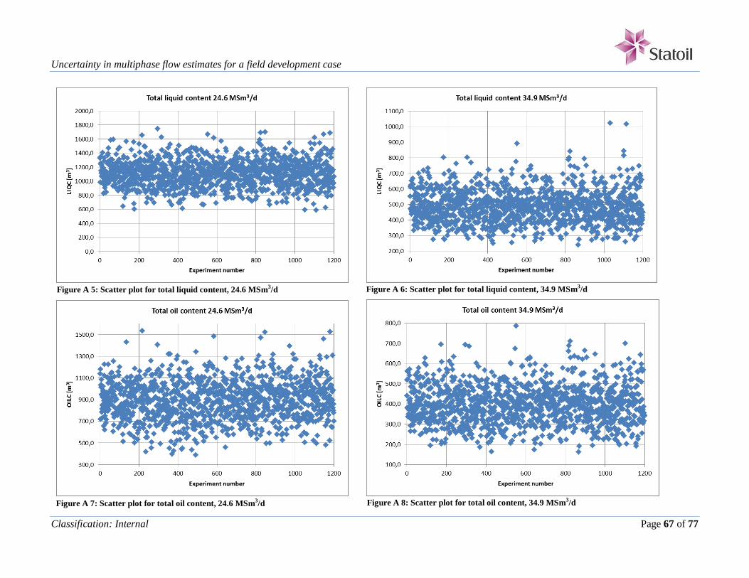
Uncertainty in multiphase flow estimates for a field development case
Classification: Internal Page 67 of 77
Figure A 6: Scatter plot for total liquid content, 34.9 MSm3/d
Figure A 8: Scatter plot for total oil content, 34.9 MSm3/d
Figure A 5: Scatter plot for total liquid content, 24.6 MSm3/d
Figure A 7: Scatter plot for total oil content, 24.6 MSm3/d

Uncertainty in multiphase flow estimates for a field development case
Classification: Internal Page 68 of 77
Figure A 10: Scatter plot for total water content, 34.9 MSm3/d Figure A 9: Scatter plot for total water content, 24.6 MSm3/d

Uncertainty in multiphase flow estimates for a field development case
Classification: Internal Page 69 of 77
11.2 Appendix B – Plots from the tuning sessions
List of figures
Figure B 1: Scatter plot for inlet pressure, 24.6 MSm3/d.............................................................. 70
Figure B 2: Scatter plot for inlet pressure, 34.9 MSm3/d.............................................................. 70
Figure B 3: Scatter plot for total pressure drop, 24.6 MSm3/d ..................................................... 70
Figure B 4: Scatter plot for total pressure drop, 34.9 MSm3/d ..................................................... 70
Figure B 5: Scatter plot for total liquid content, 24.6 MSm3/d ..................................................... 71
Figure B 6: Scatter plot for total liquid content, 34.9 MSm3/d ..................................................... 71
Figure B 7: Scatter plot for total oil content, 24.6 MSm3/d .......................................................... 71
Figure B 8: Scatter plot for total oil content, 34.9 MSm3/d .......................................................... 71
Figure B 9: Scatter plot for total water content, 24.6 MSm3/d ..................................................... 72
Figure B 10: Scatter plot for total water content, 34.9 MSm3/d ................................................... 72
Figure B 11: Distribution plot for inlet pressure, 24.6 MSm3/d ................................................... 73
Figure B 12: Distribution plot for inlet pressure, 34.9 MSm3/d ................................................... 73
Figure B 13: Distribution plot for total pressure drop, 24.6 MSm3/d ........................................... 74
Figure B 14: Distribution plot for total pressure drop, 34.9 MSm3/d ........................................... 74
Figure B 15: Distribution plot for total liquid content, 24.6 MSm3/d........................................... 75
Figure B 16: Distribution plot for total liquid content, 34.9 MSm3/d........................................... 75
Figure B 17: Distribution plot for total oil content, 24.6 MSm3/d ................................................ 76
Figure B 18: Distribution plot for total oil content, 34.9 MSm3/d ................................................ 76
Figure B 19: Distribution plot for total water content, 24.6 MSm3/d ........................................... 77
Figure B 20: Distribution plot for total water content, 34.9 MSm3/d ........................................... 77
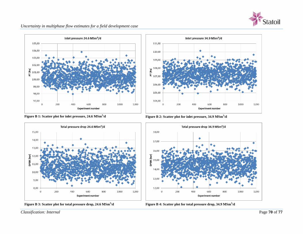
Uncertainty in multiphase flow estimates for a field development case
Classification: Internal Page 70 of 77
Figure B 1: Scatter plot for inlet pressure, 24.6 MSm3/d Figure B 2: Scatter plot for inlet pressure, 34.9 MSm3/d
Figure B 3: Scatter plot for total pressure drop, 24.6 MSm3/d Figure B 4: Scatter plot for total pressure drop, 34.9 MSm3/d
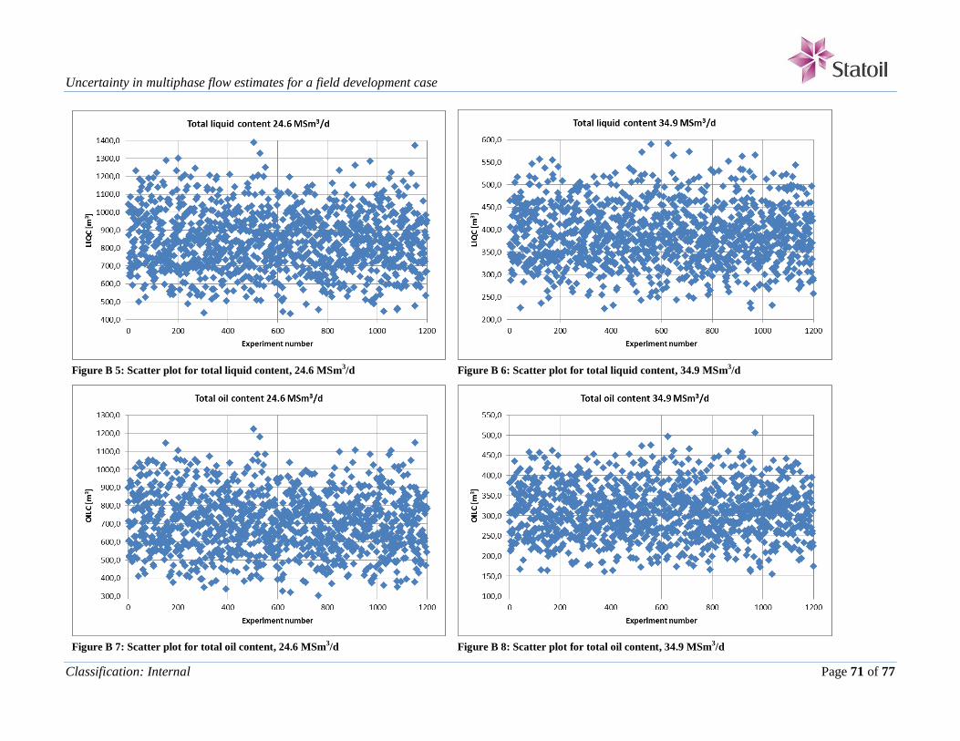
Uncertainty in multiphase flow estimates for a field development case
Classification: Internal Page 71 of 77
Figure B 5: Scatter plot for total liquid content, 24.6 MSm3/d Figure B 6: Scatter plot for total liquid content, 34.9 MSm3/d
Figure B 7: Scatter plot for total oil content, 24.6 MSm3/d Figure B 8: Scatter plot for total oil content, 34.9 MSm3/d

Uncertainty in multiphase flow estimates for a field development case
Classification: Internal Page 72 of 77
Figure B 9: Scatter plot for total water content, 24.6 MSm3/d Figure B 10: Scatter plot for total water content, 34.9 MSm3/d

Uncertainty in multiphase flow estimates for a field development case
Classification: Internal Page 73 of 77
Figure B 11: Distribution plot for inlet pressure, 24.6 MSm3/d
Figure B 12: Distribution plot for inlet pressure, 34.9 MSm3/d

Uncertainty in multiphase flow estimates for a field development case
Classification: Internal Page 74 of 77
Figure B 13: Distribution plot for total pressure drop, 24.6 MSm3/d
Figure B 14: Distribution plot for total pressure drop, 34.9 MSm3/d

Uncertainty in multiphase flow estimates for a field development case
Classification: Internal Page 75 of 77
Figure B 15: Distribution plot for total liquid content, 24.6 MSm3/d
Figure B 16: Distribution plot for total liquid content, 34.9 MSm3/d

Uncertainty in multiphase flow estimates for a field development case
Classification: Internal Page 76 of 77
Figure B 17: Distribution plot for total oil content, 24.6 MSm3/d
Figure B 18: Distribution plot for total oil content, 34.9 MSm3/d

Uncertainty in multiphase flow estimates for a field development case
Classification: Internal Page 77 of 77
Figure B 19: Distribution plot for total water content, 24.6 MSm3/d
Figure B 20: Distribution plot for total water content, 34.9 MSm3/d
Recommended