Download pdf - UC DAVIS NMR FACILITY VNMRJ SHORT MANUAL FOR VARIAN… · Varian/Agilent NMR spectrometers housed in the Chemistry complex managed by the UC Davis NMR Facility. For detailed help

1

UC DAVIS NMR FACILITY

VNMRJ SHORT MANUAL

FOR VARIAN/AGILENT NMR SPECTROMETERS

TABLE OF CONTENTS

Disclaimer ........................................................................................... 2

Conventions ........................................................................................ 2

Routine 1D NMR Experiments

Procedure for acquiring 1D Proton spectrum .................................... 3

Procedure for acquiring routine 1D Carbon spectrum ..................... 12

Common 2D NMR Experiments

Procedure for acquiring 2D COSY spectra ....................................... 15

Procedure for acquiring 2D HSQC spectra ....................................... 17

Procedure for acquiring 2D HMBC spectra ...................................... 18

Advanced 1D NMR Experiments

Determining 90 pulse widths ........................................................... 19

Procedure for T1 measurement .......................................................... 21

Procedure for T2 measurement .......................................................... 23

Procedure for Solvent Suppression / Presaturation ........................... 24

Procedure for 1D NOESY ................................................................. 26

1D Carbon DEPT: Multiplicity Editing ........................................... 29

Probe Tuning

Probe Tuning: 600 VNMRS, Chem 93 ............................................ 6

Probe Tuning: 300 Mercury Plus, Chem Annex .............................. 32

Probe Tuning: 300 Mercury, Chem 93 ............................................. 36

Troubleshooting Guide ...................................................................... 40

List and Brief Description of Important Commands ......................... 45

Date of Last Update: January 17th, 2017

2

Brief VnmrJ User Guide for Varian NMR Spectrometers

600 VNMRS, 300 Mercury, 300 Mercury Plus

DISCLAIMER

This document is intended to be a brief, bare-bones user’s guide for NMR data collection using the Varian/Agilent NMR spectrometers housed in the Chemistry complex managed by the UC Davis NMR Facility. For detailed help with both routine and advanced NMR experiments, please consult Agilent’s VnmrJ User Guides, which can be found within the Resources tab on our website, nmr.ucdavis.edu.

CONVENSIONS

Keyboard input is shown as boldface type in this manual. Note that in VnmrJ the “enter” key must be used after the command is typed; this is assumed through-out this manual and “enter” key strokes are not given explicitly. Commands in VnmrJ are typed in on the command line near the top of the VnmrJ window; again this is assumed and will not generally be stated explicitly herein. LMB, MMB, and RMB are used to indicate actions of the left, middle, and right mouse button respectively. On a PC the mouse wheel acts as the MMB. Click, and double click refer to pressing the LMB.

GENERAL PROCEDURE FOR ROUTINE WORK

You will find that the general procedure for acquiring NMR data on all NMR spectrometers is essentially the same. The general procedure is as follows:

1 Sample Preparation 2 Login and Startup 2 Setup Initial Parameters 3 Insert Sample 4 Lock onto Solvent 5 Tune the Probe 6 Shim 7 Check Acquisition parameters 8 Check Receiver Gain 9 Acquire 10 Process Data 11 Remove Sample 12 Logout, Sign Logbook

http://www.nmr.ucdavis.edu/

3

Experiment: Routine Proton NMR

Instrument: 600 VNMRS, 400 Inova, 300 Mercury, 300 Merc Plus

SAMPLE PREPARATION 1) Dissolve your sample in an appropriate deuterated NMR solvent. Make sure

there is no un-dissolved material. If there is, you will need to either centrifuge or filter your sample to remove crystals/debris.

2) Transfer about 600 uL of solvent into a clean NMR tube. We recommend high-quality NMR tubes - rated 600 MHz or higher, but economy tubes will be OK for routine work at lower fields (400 MHz and below). Your sample height should be about 5 cm.

LOGIN AND STARTUP

1) Log In: Log into your user account. a) User ID: Use your assigned user ID. This is typically issued by advisor name

or your Kerberos ID. Example: shaw002 b) password: 1gochem This is the default password for all users

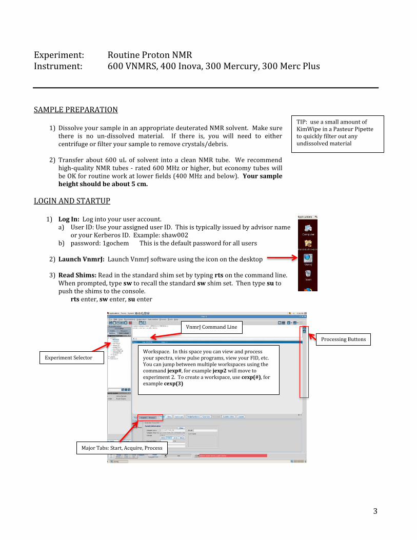
2) Launch VnmrJ: Launch VnmrJ software using the icon on the desktop

3) Read Shims: Read in the standard shim set by typing rts on the command line. When prompted, type sw to recall the standard sw shim set. Then type su to push the shims to the console.

rts enter, sw enter, su enter

TIP: use a small amount of KimWipe in a Pasteur Pipette to quickly filter out any undissolved material

VnmrJ Command Line

Experiment Selector

Major Tabs: Start, Acquire, Process

Workspace. In this space you can view and process your spectra, view pulse programs, view your FID, etc. You can jump between multiple workspaces using the command jexp#, for example jexp2 will move to experiment 2. To create a workspace, use cexp(#), for example cexp(3)

Processing Buttons

4

SET INITIAL PARAMETERS

Option 1: Load generic Proton parameters using the PROTON macro

1) In the VnmrJ command line, type PROTON followed by “enter” to load the default Proton acquisition and processing parameters. Alternatively, select the PROTON button on the left hand side under common experiments, or select Experiments -> PROTON from the menu at the top.

Option 2: Open an old Proton experiment

1) Select File -> Open, or hit the Open icon

2) Make sure the file format is .fid

3) Locate a previously saved proton NMR experiment, and select Open. This will load the raw and processed data as well as all of the acquisition and processing parameters. You can write over this data and simply use the acquisition and processing parameters.

IMPORTANT: There are two main philosophies on how to set up your initial parameters. 1 – Read in a generic parameter set, and 2 – load an old spectrum. Both methods are described below.

5

INSERT YOUR SAMPLE 1) Type e on the command line to remove the dummy sample from the

magnet 2) Remove dummy sample from the spinner, and replace with your sample 3) Adjust the sample height using the depth gauge 4) Remove fingerprints and debris from the NMR tube using a Kimwipe 5) Carefully place your sample into the magnet. It should float on a bed of air 6) Type i to insert your sample. You should hear some clicking noises

when the spinner settles correctly inside the magnet.

LOCK, TUNE, SHIM

1) LOCK: Under the Start tab and Sample Info, select your solvent. Then under Start tab and Lock, select Find Z0.

Check that the spectrometer has successfully locked by noting the Lock level. Any value greater than 10% means you are locked. Ideally your lock level should be around 70%. You can adjust the lock power and lock gain using the left and right mouse buttons. If you are having trouble locking, the issue could be many: lock phase, sample preparation, current shims, etc… The issue is rarely hardware related. Please consult the VnmrJ Troubleshooting Guide for help

Start Tab

Step 1 Step 2

Use enough sample so that your sample height fills this window (about 5 cm tall). Typically this is about 600 uL of solvent

Select your solvent using the icons, or using the drop-down list. Select Find Z0 to lock

onto your deuterated solvent.

6

2) TUNE: 600 MHZ VNMRS System Only. For other Varian systems, see Tuning training guide. Type trtune in the VnmrJ command line. Make sure to check the number of traces, and that the correct channels are designated. Typically, channel 1 is H1, channel 2 is 13C, and you select 2 as #Traces. The blue line is for the 1H channel, and the green line is for the X channel (typically set to 13C).

3) SHIM: If you have not already done so, make sure you have read in the default sw shim set (see section B3): “rts” enter, “sw” enter, “su” enter. Then, navigate to the Start / Shim tab. Maximize the value of the lock level, indicated by the dial, by changing the Z1, Z2 and maybe Z3 shims. Increase or decrease the shim values by right-clicking or left-clicking on the shim buttons.

Note, if the lock level rises to over 100%, you must drop the lock power and gain. Left-click on the Lk power and Lk gain buttons until the lock level drops to around 60%, then continue shimming. If you have the time, and you want ideal lineshape, you should try gradient shimming after manual shimming. To perform Gradient shimming, simply press the Gradient shim icon. This process usually takes anywhere between 30 seconds and a few minutes. When it has completed, you will be returned to your data set.

1H Trace (Blue). Use the tuning and matching knobs to make the dip as low as possible at the proton resonant frequency indicated by the center line. Note, the green trace is for your broadband channel, typically 13C. You can tune both channels at the same time if you wish.

Choose number of traces, and hit Start. When you are done, hit Stop and then Quit to return to your experiment.

This is the lock level: maximize this value for optimal shims

Right-click or left-click on the Z1 shim to maximize the lock level. Then do the same for Z2, Z1 again, and Z3 if you like. Typically, Z1 and Z2 are enough.

Select H1 and any additional nuclei if desired.

7

CHECK ACQUISITION PARAMETERS

1) Navigate to the Acquire / Default tab 2) Check important acquisition parameters (number of scans, spectral width, recycle delay) 3) Modify acquisition parameters if desired.

Note, many more acquisition parameters can be found under various sections of the Acquire tab including the carrier frequency, the powers and pulse lengths, decoupling parameters, and more. Please ask NMR Facility Staff for help if you wish!

CHECK RECEIVER GAIN

1) Receiver gain will be checked automatically during data acquisition if you select the Autogain option in the Default H1 tab. If you wish, you can deselect this option and manually set your receiver gain.

ACQUIRE YOUR DATA

1) Type ga or go on the VnmrJ command line, or select the Go button. Note, ga will acquire your data and perform a Fourier transform when completed, while go will acquire your data but not perform the Fourier transform.

Select Autogain

Check number of scans and recycle delay. Default is 8 scans, 1 second d1

Check spectral width. Default is -2 to 14 ppm

Acquire Tab

8

INITIAL DATA PROCESSING

1) Perform a weighted Fourier transform by typing wft on the command line. 2) Perform automatic phasing of your data by typing aph on the command line 3) View your full spectral window by typing f full on the command line, or by

using the navigation buttons.

MANUAL PHASE ADJUSTMENT

1) Often times, automatic phasing will not do an adequate job. To perform manual phasing, select the Adjust Phase button

2) Left-click and hold on the most upfield peak. Move the curser up or down to phase this peak for absorptive mode. Ignore the downfield peaks

3) Then right-click and hold on the downfield region. Move the curser up or down to phase the downfield peaks for absorptive mode.

4) If needed, re-phase the upfield peaks with left-clicking and moving up or down.

Process Tab

When you are done, hit the redraw button.

Spectral viewing buttons

Data processing buttons, including integration mode, phasing, and peak picking.

Step 2: Left-click and hold on the most upfield region, and move the curser up or down to phase this region.

Step 1: Enter phasing mode by hitting this icon

Step 3: Right-click and hold on the most downfield region, and move the curser up or down to phase this region. Repeat step 2 if needed.

9

PEAK PICKING

1) Navigate to the Process tab 2) Define the peak threshold using the Show/Hide Threshold button, and

using the left mouse button to define the threshold. Peaks that show above the defined threshold will be found for peak picking

3) Hit the Pick Peaks button

Peak Picking buttons.

Define threshold using the left mouse button

10

INTEGRATION

1) Navigate to the Process / Integration tab 2) Enter Integration mode using the Integration button

You may have to initially clear all integrals. To do so, cycle through the options in Integration mode until you see the Delete integrals option. Then cycle through the integration options again by selecting Hide Integrals, enter integration mode, and finally select the Cut Integrals icon.

3) Defining Integration Regions: You should see an unbroken green line across you entire spectrum. This green line represents the current integration regions. To define your true integration regions, use the left mouse button (LMB) while in Cut Integrals mode, and click once on the left side of your peak, and again on the right side of your peak. Repeat for all peaks of interest.

4) Calibrating Integrals: Navigate to Process / Integration tab. Exit out of integration mode by selecting the Hide Integrals button. Use the LMB to select the integral you will use for calibration. You should have only one red curser through the selected integral. Then under the Set Integral Area option, select Single Peak, and set the desired integral value. All integrals will then be calibrated based on selected integral.

PLOTTING

1) To create a hard plot, type the following on the VnmrJ command line pl pscale pir ppa page

Integration buttons.

Hide Integrals

Delete Integrals

Use the Cut Integrals button and the LMB to cut the integration window on the left and right sides of your peaks of interest. When done, select Hide Integrals button.

NOTE: see appendix VnmrJ commands list under 1D Plotting for other plotting options. The command pl, pscale, and page are all necessary. If you wish to also plot peak lists, integral regions, etc. you can add those options as well.

Note, you will have to hit this button multiple times to cycle between different options within integration mode.

11

SAVING YOUR DATA

1) To save your FID, hit the Save icon. The default data directory is /home/username/vnmrsys/data 2) Title your FID appropriately, but do not use spaces or special characters. Note, if you wish to use google

drive upload, you must save your FID directly to the home/username/vnmrsys/data directory (no sub-folders), otherwise you risk the backup macro missing your data. Press Save to save your FID

UPLOAD DATA TO GOOGLE DRIVE

1) Type the command backup into the VnmrJ command line. You will see the blue status bar go from solid blue to blue/light blue stripes. When the bar turns back to solid blue, your data has been uploaded to google drive under your designated folder.

TRANSFERING YOUR DATA TO KONA

1) Navigate to your data directory. Default data directory is

/home/username/vnmrsys/data 2) Open up the KONA FTP server. You should have a link set on

your desktop. If not, you can open up KONA the following way: a) Navigate to Places / Connect To Server b) Select Custom Location c) In the url, type: sftp://[email protected] d) Add bookmark, and call the bookmark KONA e) Select Yes Connect Anyways (if prompted) and enter the

KONA password. This password is posted at each instrument

3) Drag and drop, or copy/paste your data into your folder on KONA. You can access your data on the FTP server from anywhere on campus.

REMOVE YOUR SAMPLE

1) Type e on the VnmrJ command line 2) Remove your sample, and replace with the dummy sample into the spinner 3) Place the dummy sample (with spinner) onto the top of the bore, and then type i to stop the air flow.

LOGOUT AND SIGN LOGBOOK

1) Close VnmrJ and any other applications 2) Log out of your linux user account 3) Sign the logbook 4) Clean up the workspace

Exit Procedure

12

Experiment: Routine Carbon NMR

Instrument: 600 VNMRS, 300 Mercury, 300 Merc Plus

Before collecting 13C NMR, it is suggested you first collect a routine 1H experiment. After you have collected your Proton NMR experiment, and saved your data, you can proceed with 13C NMR setup and acquisition. Note, for 13C NMR you will need at least 10 mg to obtain decent signal to noise in a reasonable timeframe. Dissolve your sample in an appropriate deuterated NMR solvent. Make sure there is no un-dissolved material. If there is, you will need to either centrifuge or filter your sample to remove crystals/debris.

SAMPLE PREPARATION

LOGIN AND STARTUP

INSERT YOUR SAMPLE

LOCK, SHIM, TUNE

SET INITIAL PARAMETERS

1) Be sure that your PROTON data is saved

2) Load default CARBON acquisition and processing parameters over the top of your saved Proton data

by typing CARBON on the VnmrJ command line, or selecting CARBON from the experiment selector.

3) Edit the default acquisition parameters if desired. The default experiment will collect 256 scans, which takes approximately 10 minutes.

If you have not already collected a Proton NMR experiment, follow procedures in the Routine Proton guide. Make sure you have tuned 13C in addition to 1H.

13C pulse program with 1H decoupling and NOE is shown here. To display any pulse program, type dps on the VnmrJ command line

Check default acquisition parameters, and edit if necessary. Default is 256 scans, -15 to 235 ppm spectral window, 1 second relaxation delay, and using 1H decoupling and NOE enhancement. This is adequate in most situations assuming high sample concentration.

13

CHECK ACQUISITON PARAMETERS

1. Navigate to Acquire / Acquisition tab, and edit default acquisition parameters if necessary. It may be useful to change the number of scans to some high value (1024 or 2048 is common). You can always stop your acquisition after you have adequate signal to noise. Check the expected experiment time by typing time on the VnmrJ command line

2. Change the block size to 16. You can perform a Fourier transform of your FID after each block is completed.

ACQUIRE YOUR DATA

1) To start data acquisition, type go or ga on the command line, or hit Go. Note, you can perform a Fourier transform after each block is completed. During your acquisition, you will see a message after every block is completed. For example, if your block size is set to 16, after 16 scans you will see a message BS 1 completed, and BS 2 completed after 32 scans, and so on. Type wft to perform the transform and view your spectrum.

2) If you are satisfied with your signal to noise before your experiment has completed, you can stop

data acquisition by typing aa on the VnmrJ command line, or by hitting the Stop button.

Leave receiver gain set to 30, and Autogain off (not selected).

14

INITIAL DATA PROCESSING

1) Perform Fourier transform by typing wft on the command line 2) Perform automatic phasing of your data by typing aph on the command line 3) View your full spectral window by typing f full on the command line, or by using the navigation buttons.

MANUAL PHASE ADJUSTMENT

If needed, you can manually adjust the phasing of your C13 spectrum in the same manor as for H1 phase adjustment. See manual phase adjustment from the Proton guide for details.

PEAK PICKING Perform 13C Peak Picking in the same manor as for your 1H experiment. See peak picking from the Proton guide for details.

PLOTTING To create a hard plot, type the following on the VnmrJ command line

pl pscale pll ppa page

SAVE YOUR DATA TRANSFER YOUR DATA TO GOOGLE DRIVE REMOVE YOUR SAMPLE LOGOUT AND SIGN LOGBOOK

Process Tab

NOTE: see appendix VnmrJ commands list under 1D Plotting for other plotting options. The command pl, pscale, and page are all necessary. If you wish to also plot peak lists, acquisition parameters, etc. you can add those options as well.

15

Experiment: Routine 2D NMR Experiments: COSY, HSQC, HMBC

Instrument: 600 VNMRS, 300 Mercury, 300 Merc Plus

Before you start: Tuning: It is extremely important that you tune and match the probe for all nuclei used in your experiments before acquiring any 2D NMR experiment. These 2D pulse programs rely on accurate 90 and 180 pulses. If you have not tuned the probe for your specific sample, these calibrated pulses may not be correct, and your data will likely be useless. For probe tuning, consult the tuning guide: Tuning 600 VNMRS, Tuning 300 Merc Plus (Annex), Tuning 300 Mercury (Room 93). 90 Pulses: In most cases, assuming you have tuned the probe, the default pulselengths will work for your sample. However, sometimes even if the probe is tuned properly, the default pulse lengths will not be accurate. Thus, you may benefit from identifying accurate 90 and 180 pulselengths before data acquisition. See guide for Calibrating 90 Pulses for details. _____ Experiment: (HH) COSY: Gained Information: The COrrelation SpectroscopY (COSY) NMR experiment is a proton-detected 2D experiment that shows you protons that are J-coupled. You will see your 1H spectrum on both axis, and you will see a cross peak for any protons that are J-coupled. Note, the Double Quantum Filtered COSY (DQF-COSY) often gives cleaner results than the regular COSY, but at a cost of reduced signal intensity. It is recommended that you use the DQF-COSY if you have good sample concentration, and you observe sharp singlets (ie methyls) in your 1H spectrum. Procedure:

1. Collect a routine 1H NMR spectrum. Be sure to lock, tune the probe, shim. 2. Optimize spectral width

Perform Fourier transform of your data with wft, view the full spectrum by typing f full, and phase your data with aph

Use LMB and RMB to set cursors at about 1 ppm on either side of your most downfield and most upfield resonances

Move your spectral window to the area enclosed by your cursers by typing movesw in the VnmrJ command line

Re acquire your data by typing ga or go. Your spectral width should now be based on your selection 3. Move your FID to a new workspace

Say you collected 1H in experiment 1. Move this data into experiment 2 by typing mf(1,2) In this example, if experiment 2 is not available you must create it by typing cexp(2) Join experiment 2 by typing jexp2 Process the FID in the copied experiment by typing wft

4. Load COSY default acquisition and processing parameters. Note, this method will keep your lock parameters, referencing, spectral width and pulse lengths from your 1H experiment in previous steps

The recommend COSY experiment is the gradient-selected cosy: gCOSY. Load default parameters in one of the following equivalent ways:

i. type in the COSY macro in the VnmrJ command line:

COSY 600 VNMRS gCOSY 300 Merc 93 COSY 300 Merc Annex gCOSY

16

ii. navigate to Experiments > Homonuclear Correlation > Gradient Cosy iii. under Experiment Selector / Common, hit the (HH)gCOSY macro button

Note, if your sample has sharp singlet proton resonances, and sample concentration is not an issue, your data will look much nicer if you use the Double Quantum Filtered COSY experiment. You will not see methyl peaks or other singlets, which are not of interest for a COSY experiment anyways. To load this experiment:

i. Type in the DQF-COSY macro into the VnmrJ command line:

ii. navigate to Experiments > Homonuclear Correlation > Gradient DQF COSY iii. under Experiment Selector / Liquids / (HH)Homo2D, hit the gDQCOSY option

5. Check and modify acquisition parameters Navigate to Acquire / Acquisition Enter 1024 complex points in F2 (your direct dimension) It is recommended to acquire at least 2 scans and at least 256 points in F1 (your indirect dimension.

512 is better if you have the time!). Change number of scans and points in F1 as you see fit. Use multiples of 2 for number of scans, and increments of at least 32 for points collected in F1.

The default relaxation delay is 1 second. For best results, change this to 1.5 or 2 seconds. Check the experiment time by typing time on the VnmrJ command line. Modify number of scans and

F1 points if necessary. 6. Acquire your data

Type go or ga on the command line, or hit the Acquire button 7. Process your data

When your acquisition is complete, navigate to Process tab and hit the Autoprocess button 8. Save your data, and upload to KONA

DQF-COSY 600 VNMRS gDQCOSY 300 Merc 93 DQCOSY 300 Merc Annex gDQCOSY

17

Experiment: (HC) HSQC: Gained Information: The Heteronuclear Single Quantum Correlation (HSQC) NMR experiment is a proton-detected 2D experiment that shows you 1H / 13C connectivity. You will see your 1H spectrum as your F2 axis and your 13C spectrum as your F1 axis, and you will see a cross peak for any 1H connected to a 13C that is one bond away. The HSQC is often faster to acquire and more informative than the 1D 13C DEPT experiment, and the same information is obtained. Procedure:

1. Collect a routine 1H NMR spectrum. Be sure to lock, tune the probe FOR BOTH 1H AND 13C, shim. 2. Optimize spectral width





Say you collected 1H in experiment 1. Move this data into experiment 2 by typing mf(1,2). This way you will not overwrite your original 1H data, and you can jump back and forth between your Proton and your HSQC experiments by typing jexp1 and jexp2, respectively.

In this example, if experiment 2 is not available you must create it by typing cexp(2) Join experiment 2 by typing jexp2 Process the FID in the copied experiment by typing wft

4. Load HSQC acquisition and processing parameters Type the following into the VnmrJ command line, depending on which instrument you are using:

5. Check and modify acquisition parameters Navigate to Acquire / Defaults tab Check your 13C spectral width to make sure you capture all expected 13C resonances with attached

protons. Default is -10 to 160 ppm. Keep in mind, you will only be observing 13C resonances with attached protons.

i. Example 1: Carbonyl peaks near 170 ppm can be ignored. ii. Example 2: Aldehydes show up in the 190-200 ppm region and have an attached proton(s),

so you will have to expand your spectral width to capture these types of carbons. Navigate to Acquire / Acquisition Enter 1024 complex points in F2 (your direct dimension). You should shoot for an acquisition time

in your direct F2 dimension of about 0.2 – 0.3 seconds. It is strongly recommended to acquire at least 4 scans and at least 256 points in F1 (your indirect

dimension). You will likely need more unless your sample concentration is extremely high. Change number of scans and points in F1 as you see fit. Use multiples of 4 for number of scans, and increments of at least 32 for points collected in F1. Check your experiment time by typing time on the command line.





600 VNMRS gHSQCAD 300 Merc 93 Does Not Work 300 Merc Annex gHSQC

18

Experiment: (HC) HMBC: Gained Information: The Heteronuclear Multiple Bond Correlation (HMBC) NMR experiment is a proton-detected 2D experiment that shows you 1H / 13C multiple-bond connectivity. You will see your 1H spectrum as your F2 axis and your 13C spectrum as your F1 axis, and you will see a cross peak for any 1H / 13C pair that are multiple bonds away, typically 3 to 5 bonds. Procedure:

1. Collect a routine 1H NMR spectrum. Be sure to lock, tune the probe FOR BOTH 1H AND 13C, shim. 2. Optimize spectral width





Say you collected 1H in experiment 1. Move this data into experiment 2 by typing mf(1,2). This way you will not overwrite your original 1H data, and you can jump back and forth between your Proton and your HMBC experiments by typing jexp1 and jexp2, respectively.

In this example, if experiment 2 is not available you must create it by typing cexp(2) Join experiment 2 by typing jexp2 Process the FID in the copied experiment by typing wft

4. Load HMBC acquisition and processing parameters Type the following into the VnmrJ command line, depending on which instrument you are using.

Alternatively, find the equivalent experiment from the Experiment Selector:

5. Check and modify acquisition parameters Navigate to Acquire / Defaults tab Check your 13C spectral width to make sure you capture all expected 13C resonances that you would

see in your routine 1D 13C spectrum. Default is -10 to 220 ppm. If you have collected your 13C spectra, use this information to properly select your 13C spectral width in your HMBC.

Navigate to Acquire / Acquisition Enter 2048 complex points in F2 (your direct dimension). You should shoot for an acquisition time

in your direct F2 dimension of about 0.3 – 0.4 seconds. The HMBC is not a very sensitive experiment. You will likely need high sample concentration (25

mg/mL or greater). It is strongly recommended that you acquire at least 32 scans and at least 128 points in F1 (your

indirect dimension). Change number of scans and points in F1 as you see fit. Use multiples of 4 for number of scans, and increments of at least 32 for points collected in F1. This should take about 3 hours of experiment time.





600 VNMRS gHMBCAD 300 Merc 93 Does Not Work 300 Merc Annex gHMBC

19

Experiment: Advanced 1D NMR Experiments: Pulse Calibration, T1, T2, Solvent Presaturation, DEPT

Instrument: 600 VNMRS, 400 Inova, 300 Mercury, 300 Merc Plus

Before you start: Tuning: It is extremely important that you tune and match the probe for all nuclei used in your experiments before acquiring any 2D NMR experiment. These 2D pulse programs rely on accurate 90 and 180 pulses. If you have not tuned the probe for your specific sample, these calibrated pulses may not be correct, and your data will likely be useless. For probe tuning, consult the tuning guide: Tuning 600 VNMRS, Tuning 300 Merc Plus (Annex), Tuning 300 Mercury (Room 93). 90 Pulses: In most cases, assuming you have tuned the probe, the default pulselengths will work for your sample. However, sometimes even if the probe is tuned properly, the default pulse lengths will not be accurate. Thus, you may benefit from identifying accurate 90 and 180 pulselengths before data acquisition. See guide for Calibrating 90 Pulses for details.

Experiment: Determining 90 and 180 Pulse Widths Gained Information: All advanced 1D and 2D NMR experiments rely on accurate 90 and 180 pulses to manipulate nuclear spins. If you intend to collect NMR data where the pulse program requires multiple pulses, you will need accurate pulselengths. Assuming the probehead is properly tuned, the default values will be fairly accurate. However, in some cases (salty samples for example), the default pulse widths will be far off from ideal for your sample. It is a good idea to check your pulse widths for your specific sample, as these parameters depend on sample. Procedure:

1. Collect a routine 1H NMR spectrum. Be sure to lock, tune the probe, shim. 2. Move your transmitter frequency


Use LMB to set cursor to a strong 1H resonance. This could be your solvent peak, or better yet a strong peak from your compound.

Move your carrier frequency (center of your spectrum) to the chosen resonance by typing movetof in the VnmrJ command line

Re acquire your data by typing ga or go. Your spectral width should now be based on your selection 3. Check and modify acquisition parameters

Navigate to Acquire / Acquisition Enter 1 scan, 0 steady state scans, 10 seconds relaxation delay, and turn off Autogain Check your calibrated 90 pulselength; pw90. You should expect your result to be close to the

calibrated value assuming you have tuned the probe 4. Setup parameter array (pw)

Go to Acquisition / Parameter Arrays Input pw as your array parameter. Taylor your array based on your initial guess of the 180 pulse. If

your calibrated 90 pulse is 15 microseconds, try an array that flanks the expected 180 from say 15 to 45 microseconds.

20

5. Acquire your data Type go on the VnmrJ command line. Note, do not use ga, as VnmrJ will attempt to autoprocess each

of your spectra. 6. Process your data

To process each spectrum, type wft dssh dssl on the command line. This will display each of the 15 spectra horizontally. You are looking for the null at 180 degrees.

When you find the 180, open up the Parameter Array list to see which pulselength resulted in the null. Divide this time by two, and this is your calibrated 90 time.

You may want to re-run your array with a tighter window for better accuracy. In this example, re-run from 25 to 35 us.

7. Save your data to the default data folder (/home/username/vnmrsys/data/) and upload your FID to google drive (type the command backup on the vnmrj command line)

180 null at array 10 (30 s), so 90 pulselength = 15 s

21

Experiment: T1 Measurement: Inversion Recovery Gained Information: This experiment will estimate spin-lattice (T1) relaxation times for all resonances in your Proton spectrum. This information is especially important if you wish to collect quantitative NMR spectra, where you will need a relaxation delay of at least 5x T1 for your slowest relaxing peak. Procedure:







4. Load Inversion Recovery pulse sequence Type in INVREC on the VnmrJ command line, or select 1H T1 Relaxation from the Experiment

selector 5. Check and modify acquisition parameters

Navigate to Acquire / Acquisition In most cases, you only need a crude estimate for T1. For a crude T1 estimate, enter 1 scan, 0 steady

state scans, 20 seconds relaxation delay, and turn off Autogain. Check to make sure your 90 pulse is correct.

6. Acquire your data

Type go on the VnmrJ command line. Note, do not use ga, as VnmrJ will attempt to autoprocess each of your spectra.

Enter your calibrated 90 pulse if it is different from the default

Use a long relaxation delay. 20 seconds is enough in most cases.

For a crude estimate, just enter 1 scan and 0 steady state scans. If you want to be more accurate, use at least 4 scans and 2 steady state scans.

22

7. Process your data First type wft, then display your first spectrum by typing ds(1) Navigate to Process / T1 Analysis tab Select Display Last Spectrum, phase for positive peaks Set the threshold for peaks you wish to identify T1. Select Do T1 Analysis, or type t1 on the command line Check T1 and estimated error for each peak of interest. The fitting results can be found under

Process / T1 Analysis tab.

8. Save your data to the default data folder (/home/username/vnmrsys/data/) and upload your FID to google

drive (type the command backup on the vnmrj command line)

Peaks picked by setting the threshold will be analyzed for T1 relaxation

Results of T1 Analysis are shown here

23

Experiment: Measuring 1H T2 Relaxation: CPMG Experiment Gained Information: This experiment will estimate spin-spin (T2) relaxation times for all resonances in your Proton spectrum. Procedure:







4. Load Inversion Recovery pulse sequence Type in CPMGT2 on the VnmrJ command line, or select 1H T2 Relaxation from the Experiment

selector 5. Check and modify acquisition parameters

Navigate to Acquire / Default The default acquisition parameters are sufficient for most cases. This experiment takes

approximately 8 minutes with default acquisition parameters. If you only want a crude estimate of T2, change number of scans to 1, and number of steady-state scans ss to 0.

Check minimum and maximum T2 times, and adjust if necessary. Under the Acquire / Acquisition tab, check to make sure your 90 pulse is correct. If you have

calibrated your 90 pulse, enter that value as pw90 and make sure your observe pulse is set to 90 degrees.

6. Acquire your data Type go on the VnmrJ command line. Note, do not use ga, as VnmrJ will attempt to autoprocess each

of your spectra. 7. Process your data

First type wft, then display your first spectrum by typing ds(1) Type f full to display the full spectrum Phase your peaks from spectrum 1 so that they appear positive Navigate to Process / T2 Analysis tab Select Display First Spectrum Set the threshold for peaks you wish to identify T2. Select Do T2 Analysis Check T2 and estimated error for each peak of interest. The fitting results can be found under

Process / T2 Analysis tab. 8. Save your data to the default data folder (/home/username/vnmrsys/data/) and upload your FID to google

drive (type the command backup on the vnmrj command line)

24

Experiment: Solvent Suppression: Presaturation Introduction: Solvent suppression techniques allow for NMR data collection without the need for 100% deuterated solvents. Presaturation is one of multiple solvent suppression techniques (other common methods include Watergate and Excitation Sculpting) where the major solvent peak is selectively irradiated with a long, low power RF pulse prior to full excitation and data acquisition. Most often, this is done for biological samples in 90% H2O / 10% D2O solvent systems: the 10% D2O is used for locking and shimming, while the massive 90% H2O signal is suppressed. Presaturation can also be used to suppress major impurities in a sample that may overwhelm other resonances of interest. Procedure:

1. Insert your sample, and load a routine PROTON experiment. 2. lock, tune, shim 3. Change your acquisition parameters: set ns=1, ss=0, and observe pulse pw to a small tip angle 4. Collect a single scan using go or ga, then perform Fourier transform with wft, and phase for positive peaks

with aph.

5. Move your transmitter frequency Perform Fourier transform of your data with wft, view the full spectrum by typing f full, and phase

your data Zoom into your large solvent peak, and use LMB to set cursor to the strong solvent peak that you

wish to presat. For H2O/D2O, this is near 4.7 ppm. Move your carrier frequency to the chosen peak by typing movetof in the VnmrJ command line Re acquire your data by typing ga or go. The center of your spectrum should now be based on your

selection. Re-process data with wft 6. Load PRESAT pulse sequence

Type in PRESAT on the VnmrJ command line, or select 1H PRESAT from the Experiment selector 7. Optimization of presat frequency and power using Do Scout

Navigate to Acquire / PRESAT, and select the Do Scout option.

Set the Presaturation power depending on your system. For 90% H2O / 10% D2O samples, you should set the presat power so that the presat excitation is about 25 Hz. The actual power (in dB) will depend on which instrument you are using.

Type ga or hit the Acquire button to begin the Do scout option to automatically optimize your satfreq. You should see an array similar to the one displayed here. When Do Scout has completed, you can check your optimized presaturation frequency by typing satfrq? on the command line, or by checking the Offset (Hz) in the Acquire / PRESAT tab.

Use a short tip angle, otherwise your solvent peak may be too big.

Acquire, transform, phase positive.

Set cursor here, then type movetof, and re-acquire using ga

Note, the presaturation power satpwr is initially set for suppressing small peaks, so you will have to increase the satpwr depending on your needs. For solvent systems where you are only using 10% deuterated solvent, you will need to increase the satpwr until your excitation profile is about 25 Hz. You can later adjust this for higher or lower power based on your system.

Optimal suppression here; satfeq = -154.2 Hz

25

8. Optimize acquisition parameters Set number of scans to at least 8, steady state scans to 4, enable Auto Receiver Gain Adjust your spectral width if necessary, but be careful NOT to move your carrier frequency.

9. Acquire your data Type ga on the VnmrJ command line, or hit the Acquire button.

10. Process your data as normal with wft and aph. Depending on your results, you may want to increase or decrease your presaturation power satpwr. As you increase the power, you will suppress a wider signal, but keep in mind this may also suppress some of your peaks of interest. Ideally you want to keep satpwr as low as possible while still maintaining good solvent suppression.

11. Save your data to the default data folder (/home/username/vnmrsys/data/) and upload your FID to google drive (type the command backup on the vnmrj command line)

26

Experiment: Selective 1D NOESY Experiment Gained Information: 1D NOESY experiment to illustrate protons that are near each other in space. The selective NOE experiment is commonly used to determine stereochemistry; one selectively excites a proton resonances and observes NOE transfer to nearby protons. Typically, one observes NOE peaks for proton resonances that are in a relatively rigid environment that are within 5 Angstroms of each other. Assuming you are only trying to identify NOEs for a select few resonances, this experiment is often much faster than the 2D NOESY. With any NOE experiment, you need to keep in mind that NOE depends on the molecular tumbling rate, so molecular weight is an important factor in choosing both your experiment and your acquisition parameters. NOE will be positive for small molecules (under 600 Daltons), go through a zero for medium-sized molecules (700 to 1500 Da), and become negative for larger molecules (greater than 1500 Da). For medium-sized molecules, you should try the Selective ROESY experiment, since ROE is always non-zero. You should choose your NOE mixing time based on your molecular weight. As a starting point, for small molecules try a mixing time of 0.5 seconds, medium sized molecules try 0.3 seconds, and large molecules try 0.1 seconds. Procedure: - Written for 600 MHz VNMRS. For other instruments, please ask NMRF staff.

1. Insert your sample, and load routine PROTON experiment. 2. lock, tune, shim 3. Acquire a normal 1H spectrum. Process with ft or wft, and phase with aph.

4. Copy your FID to a new workspace so that you don’t write over your 1H data. For example, copy your recently-acquired 1H data from your current worspace (eg. workspace 1)

into a new worspace (eg. workspace 2) using the command: mf(1,2). The command reads as Move FID from workspace 1 to 2. If workspace 2 is not created, you must create it with the command cexp(2). You can create as many workspaces as you like this way.

Join the selected workspace with jexp#, where # is the number of the selected workspace. In this case: jexp2

Process your FID again in the second workspace with wft and aph 5. Load 1D NOESY pulse sequence

Type in NOESY1D on the VnmrJ command line, or select 1D NOESY from the Experiment selector.

27

6. Select your 1H resonance that you wish to selectively irradiate Use LMB and RMB to zoom into the peak of interest Navigate to Acquire tab / Defaults Set the LMB at the base of your peak on the left side, and the RMB at the base of your peak at the right

side Now hit Select. This will create a selective 1H pulse that only excites the peak of interest.

7. Edit 1D NOESY acquisition parameters, if desired Check NOE mixing time. For most small molecules, 300 – 500 milliseconds is good. Adjust number of scans – the more the better. It is suggested that you at minimum square the

number of scans necessary for a good 1H spectrum. For a 25 mg/mL sample of cinchonidine in CDCl3, 64 scans is OK but 128 would be better.

For better results, increase steady state scans ss and relaxation delay d1, if you have time. Try ss=32 and d1=2

1: Set left mouse curser and right mouse cursers at the base of the peak of interest

2: Hit Select. This will create a shaped pulse based on where you set your cursors in step 1. If you mess up, just hit CLEAR and try again.

28

8. Acquire your data Hit the GO button. Note, the shaped pulses are generated when you hit this GO button.

Typing go into the command line will not generate these shaped pulses and the experiment will fail.

9. Process your data as normal with wft and aph. You will likely need to move the baseline up to midway so you can see peaks phased up and down.

Use the Hand icon and drag the baseline up. The selectively-irradiated peak should be phased down, while the peaks experiencing NOE transfer

will be phased up. If you notice peaks with anti-phase character, they are likely due to J-Coupling and not from NOE.

10. Save your data using the Save As button. Upload to google drive using the backup command. 11. Log out, sign the log book when you are done.

Selectively irradiated resonance phased down

Nearby protons show NOE correlations. The relative intensity is correlated to the distance from the irradiated resonance. You should only expect to observe NOE for protons that separated by under ~5 Angstroms.

29

Experiment: 1D Carbon DEPT NMR: DEPT135 and DEPT90

Introduction: DEPT: Distortionless Enhancement by Polarization Transfer. Carbon signals are enhanced and edited through their attached protons. With the DEPT135 experiment, delays are set such that CH and CH3 signals are phased up, and CH2 phased down. DEPT90 only shows CH signals. When you call in the DEPT experiment in VnmrJ, by default there will be 4 experiments queued: Standard 13C, DEPT135, DEPT90, and DEPT45. This option takes 4x longer than the more common DEPT135 experiment. Be mindful of which DEPT spectral editing parameters you wish to collect. We recommend you individually collect standard 13C and DEPT135 data, and additional multiplicity edits if you wish. Before collecting 13C NMR data including DEPT experiments, it is suggested you first collect a routine 1H experiment. After you have collected your Proton NMR experiment, and saved your data, you can proceed with 13C NMR setup and acquisition. Note, for 13C NMR you will need at least 10 mg to obtain decent signal to noise in a reasonable timeframe. Dissolve your sample in an appropriate deuterated NMR solvent. Make sure there is no un-dissolved material. If there is, you will need to either centrifuge or filter your sample to remove crystals/debris.

PROCEDURE – Written for 600 MHz VNMRS. For other instruments, ask NMRF staff.

1. Insert your sample 2. Lock, tune, shim. It is imperative that both 1H and 13C channels are tuned. 3. If you have not already done so, collect routine proton experiment. Save data. 4. If you have not already done so, load and collect a routine CARBON experiment (See Routine 13C

Guide). If you have already collected, you can also load old data with File / Open or using the Open icon.

5. Process 13C data Fourier transform and autophase with wft aph View full spectrum with f full vsadj

6. If newly acquired, save your 13C data using the Save As icon. 7. Optional but recommended: Move your FID to a new workspace

Say you collected 13C in experiment 1. Move this data into experiment 2 by typing mf(1,2) In this example, if experiment 2 is not available you must create it by typing cexp(2) Join experiment 2 by typing jexp2 Process the FID in the copied experiment by typing wft

8. Optional but recommended– Define your 13C spectral window based on your recent spectrum. Use Left Mouse Button and Right Mouse Button to enclose all your 13C peaks, including TMS Type movesw on the VnmrJ command line to move the spectral width to desired window

Summary: After collecting 13C data, set LMB and RMB to enclose all peaks, including TMS. Then type movesw to set spectral width. Type DEPT to load DEPT parameters

30

9. Load the DEPT experiment over the top of your 13C data by typing DEPT on the command line, or by selecting the DEPT experiment in Experiments / X-H Multiplicity Determination / DEPT.

CHECK ACQUISITON PARAMETERS

1. Navigate to Acquire / Pulse Sequence tab 2. Select which type of spectral editing experiment you would like to collect. (eg., DEPT135, DEPT90)

Most common is to select DEPT135 experiment – CH and CH3 up, CH2 down. You can differentiate between CH and CH3 signals by collecting both DEPT135 and DEPT90 data.

3. Navigate to Acquire / Acquisition tab

Double check acquisition parameters like number of scans, spectral width, acquisition time, relaxation delay and block size. You will likely want to collect 256 scans or more for high quality data. You can also set number of scans to a high value, and just stop acquisition when data is satisfactory.

ACQUIRE YOUR DATA

1. To start data acquisition, type go or ga on the command line, or hit Go. Note, you can perform a Fourier transform after each block is completed. During your acquisition, you will see a message after every block is completed. For example, if your block size is set to 8, after 8 scans you will see a message BS 1 completed, and BS 2 completed after 16 scans, and so on. Type wft to perform the transform and view your spectrum.

Useful tip: set Block size to some small number (eg., 8) so you can check Fourier transform after every block..

For DEPT135, select here. If you wish, you can collect Full Edit, but this collects 4 spectra so it takes 4x longer.

Check number of scans. In this case, 64 scans was just enough to get noisy data on a 25 mg/mL sample in CDCl3

31

2. If you are satisfied with your signal to noise before your experiment has completed, you can stop data acquisition by typing aa on the VnmrJ command line, or by hitting the Stop button.

PROCESS YOUR DATA

1. Perform Fourier transform by typing wft on the command line 2. Perform automatic phasing of your data by typing aph on the command line 3. View your full spectral window by typing f full on the command line, or by using the navigation

buttons. 4. Move the baseline to the middle of the screen by selecting the Hand icon, and dragging the spectrum

up.

5. Save your data using the Save As icon. Be sure to save to the default folder, (/home/username/vnmrsys/data/) otherwise data will not properly be uploaded to google drive.

6. Upload your FID to google drive (type the command backup on the vnmrj command line) 7. Remove sample, close VnmrJ, log out, sign log book.

Process Tab

DEPT135 on 25 mg/mL Quinine in CDCl3. 64 scan averages were collected, which were not enough in this case. CH and CH3 are phased up, CH2 down, and quat carbons are not observed.

32

Probe Tuning Guide: Proton 300 Mercury Plus (Chem Annex) Step 1: Getting Started

• Load a PROTON experiment in VnmrJ • Type su on the command line • Insert your sample • Make sure that the Proton tuning rod is in the UP position

Step 2: Move the Cables

1H / 19F Tune (Red).

This piece slides up and down: UP is for Proton, DOWN is for Fluorine. Make sure this is in UP position

Move High Band from J5102 to Tune J5402

Move High Band TX from J5602 to Tune 5604

Move High Band Out from J5103 to Q-

Tune J5403

33

Step 3: Tune the Probe • Make sure the front of the tuning interface is set to Tune mode • Type btune on the VnmrJ Command line. You should see a message “Tuning H1, type tuneoff when done”

Step 4: When you are Done

• Type tuneoff in the VnmrJ command line • Move all cables to their original positions • Proceed with normal data acquisition (Lock, Shim, etc)

• Set to Tune Mode

• Set attenuation so that the LED display reads numbers between 20 and 100

A. Carefully rotate the Proton Tuning knob while watching the LED display. If the display reads a lower number, you are tuning successfully.

Note, rotate slowly and carefully. If you feel a change in resistance, stop and rotate the other direction. Do not over-turn, you can easily damage the probe!

B. When you have minimized the reflected power with the Tune knob, you can try to match the probe for a better response. Turn the match very slowly. Only a quarter turn or half turn may be enough to reach optimal match.

C. If you have changed the match, return to the Tune and again optimize for lowest reflected power

A: 1H Tuning Knob B: 1H Match Knob

Counter for X-Channel Tuning. Should read 68 for 4NUC mode

34

Probe Tuning Guide: X-Channel (Carbon, Phosphorus) 300 Mercury Plus (Chem Annex)

Step 1: Getting Started

• Load a CARBON or PHOSPHORUS experiment in VnmrJ • Type su on the command line • Insert your sample • Make sure that the Tuning Counter reads 68, and that the X-Channel tuning rod is in the UP position


X-Channel Tune (Green).

This piece slides up and down: UP is for tuning, while DOWN will engage the gear to change the tuning counter. You want the counter to read 68. If it does not, slide the knob to the Down position, rotate until the counter reads 68, then slide back to the UP position.

• Disconnect BB cable J6001 before the filter (cable has green tape, should go directly to the probe) and move to Tune J5402

• Move Low Band TX J5603 to Tune J5604

• Move Low Band Out J5303 to Q-

Tune J5403

35

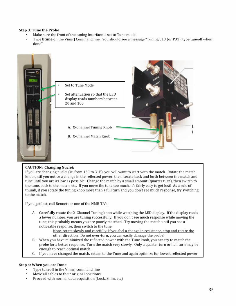
Step 3: Tune the Probe • Make sure the front of the tuning interface is set to Tune mode • Type btune on the VnmrJ Command line. You should see a message “Tuning C13 (or P31), type tuneoff when

done”



CAUTION: Changing Nuclei: If you are changing nuclei (ie, from 13C to 31P), you will want to start with the match. Rotate the match knob until you notice a change in the reflected power, then iterate back and forth between the match and tune until you are as low as possible. Change the match by a small amount (quarter turn), then switch to the tune, back to the match, etc. If you move the tune too much, it’s fairly easy to get lost! As a rule of thumb, if you rotate the tuning knob more than a full turn and you don’t see much response, try switching to the match. If you get lost, call Bennett or one of the NMR TA’s!

A. Carefully rotate the X-Channel Tuning knob while watching the LED display. If the display reads a lower number, you are tuning successfully. If you don’t see much response while moving the tune, this probably means you are poorly matched. Try moving the match until you see a noticeable response, then switch to the tune.

Note, rotate slowly and carefully. If you feel a change in resistance, stop and rotate the other direction. Do not over-turn, you can easily damage the probe!




• Set attenuation so that the LED display reads numbers between 20 and 100

A: X-Channel Tuning Knob B: X-Channel Match Knob

36

Probe Tuning Guide: Proton 300 Mercury (Chem Room 93)

Step 1: Getting Started

• Load a PROTON experiment in VnmrJ • Type su on the command line • Insert your sample • Identify the Proton Tune and Match knobs


Proton Tune knob Proton Match knob

A

B

C

A. Move High Band from J5102 to Tune J5402 (Inside Leg)

B. Move High Band TX from J5602 to Tune J5604 (Back Side) C. Move High Band Out from J5103 to Q-Tune J5403 (Back Side)

37

Step 3: Tune the Probe • Make sure the front of the tuning interface is set to Tune mode • Type btune on the VnmrJ Command line. You should see a message “Tuning H1, type tuneoff when done”



A. Carefully rotate the Proton Tuning knob while watching the needle. If the display reads a lower number, you are tuning successfully.

i. Note, rotate slowly and carefully. If you feel a change in resistance, stop and rotate the other direction. Do not over-turn, you can easily damage the probe!



A: 1H Tuning Knob B: 1H Match Knob


• Set attenuation so that the needle reads between 20 and 100

Monitor this needle while tuning and matching. Optimize for minimal reflected power.

38

Probe Tuning Guide: X-Channel (Carbon, Phosphorus, etc) 300 Mercury Plus (Chem Room 93) Step 1: Getting Started

• Load the intended experiment in VnmrJ (CARBON, PHOSPHORUS, etc) • Type su on the command line • Insert your sample • Identify the X-Channel Tune and Match knobs • Identify Probe Configurations for desired nucleus, listed at the base of the probe.


A. Move BB Probe from J6001 to Tune J5402 (Inside Leg)

B. Move Low Band TX from J5603 to Tune J5604 (Back Side)

C. Move Low Band Out from J5303 to Q-Tune J5403

(Back Side)

X-Channel Tune knob X-Channel Match knob

Nucleus Counter Capacitor Stick 13C 68 None 31P 12 None 29Si 83 None Other Check Paperwork behind the 600

A B

C

39

Step 3: Tune the Probe • Make sure the front of the tuning interface is set to Tune mode • Make sure the probe configuration is correct. For example, for 13C make sure there is no capacitor stick, and

the probe tuning counter reads near 47 (does not have to be exactly 47, this is a starting point!). If it does not read near 47, rotate the X-Channel Tuning Knob until you see the correct reading

• Type btune on the VnmrJ Command line. You should see a message “Tuning C13 (or 31P, 29Si), type tuneoff when done”



A. Set the X-Channel tuning knob so that the counter reads the suggested value. For 13C, make sure the counter reads 47, for 31P it should read 12

B. Set the attenuation on the tuning interface so that the needle reads between 20 and 100 C. Now move the X-Channel Match knob until you see a change in reflected power. Minimize reflected

power D. Now go back to the X-Channel Tune and optimize for minimal reflected power (low reading on the

needle). You may need to iterate back and forth between the match and tune for the lowest reading. Note, at attenuation level 7, the needle should read somewhere near 20 or 30 when you are

well tuned/matched

A: X-Channel Tuning Knob B: X-Channel Match Knob


• Set attenuation so that the needle reads between 20 and 100.

Monitor this needle while tuning and matching. Optimize for minimal reflected power.

40

Troubleshooting Guide

Problems during acquisition

The vast majority of VnmrJ acquisition problems are due to interrupted communications between the spectrometer's console and the host (Dell) computer. Some of these problems include:

The acquisition doesn't start when you give the go” or ga command or when you click on the [Acquire] button.

The spectrometer doesn't obey commands or buttons like [Find Z0], [Gradient autoshim], [Acquire], etc. The sample is not ejected with the [Eject] button or the e Command. The message “Setup complete” does not appear after you type su The message Active or Inactive or Interactive appears continuously on the bottom of the Vnmrj window

instead of the normal green Idle even when no acquisition or shimming is in progress. The message: “Cannot set hardware during interactive acquisition” or “Cannot do {some command} when

an acquisition is active or queued” or “sethw cannot proceed, another user's experiment is already active” or “Acquisition system is not active” appears on Vnmrj's info bar.

The lock display is slower than normal (it refreshes the image less than two times per second). The red RCVR OVFL light on the status unit adjacent to the monitor of the Inovas is continuously lit even

when no acquisition is in progress (it is normal for it to flash during pulses or to be on when the [Lock Scan] button is depressed).

To solve these problems, try the following steps, in order, until you resolve your problem:

1. Close out of VnmrJ and re-open. If that doesn’t work: 2. type abortallacqs on the command line of Vnmrj, wait not less than 1 minute and then type su. If

successful, the message “Setup complete” should appear. You will need to reload the sw shims and lock parameters and re-shim after this.

3. If the above doesn't work, you should perform an sq acqproc a. close out of VnmrJ b. right click on the desktop and open up a terminal window c. type su acqproc in the terminal window. It should say “Stopping Acquisition Communications”.

Wait until this process is complete (usually about 10 seconds) d. type su acqproc again to restart console communications. A new window with a message like

“Acquisition Console at 600 MHz ready“ might appear e. Close out of the Terminal windown and Open up VnmrJ. f. Be sure to read in the shims: rts “enter”, sw “enter, su “enter”

4. If you are still having issues, you may have to reset the console. a. Close out of VnmrJ and open up a terminal window again. b. Stop communications by typing su acqproc wait 30 seconds. c. Go to the console and find the reset button. On the 600 MHz it is inside the right door of the

console, near the bottom and to the right. On the 400 MHz it is inside the left door of the console, near the center and to the left. On the 300 MHz spectrometers it is on the back of the console. Press this reset button, and wait about 1 minute.

d. In the terminal window, type su acqproc again. e. Close out of the Terminal windown and Open up VnmrJ. f. Be sure to read in the shims: rts “enter”, sw “enter, su “enter”

5. If you are still having issues, leave a note in the logbook, and contact NMR Facility staff via phone call or email immediately so we can resolve the issue. Please consult the call-sheets posted at each instrument to determine who to call.

41

Locking and Shimming problems a) I cannot find the lock signal or lock the sample. b) The lock signal is unstable. c) Shimming is difficult.

The majority of Locking and Shimming problems come from one of two things:

1. You forgot to load in the default shims. Make sure you do this before locking. To load in the default sw shim set, type rts “enter” sw “enter“ su “enter” in the VnmrJ command line.

2. Your sample preparation is poor. If you expect your lineshape to look good after simply touching up the Z1 and Z2 shims, you must make sure your sample is prepared correctly. Here are a few suggestions for a properly prepared sample:

a. Make sure you are using a deuterated solvent. Yes, that sounds silly but... it has happened. b. Make sure your sample height is about 5 cm. Eject the sample and verify that you have enough

solvent to fill the window in the depth gauge. c. Make sure you don’t have any undissolved material in your sample. If you still have residual solid

material, go back to your lab and try to remove this material with a simple filtration or centrifugation. Often using a bit of kimwipe wadded up in the base of a Pasteaur glass pipette is enough to filter out undissolved material.

If everything is correct, it is possible that something in your solution or tube may be making the lock signal so broad that the lock level is too low to be noticed. This includes paramagnetic metals, particles in suspension, high viscosity or a bad tube. The lock parameters; Z0, lockpower, lockgain and lockphase depend on solvent characteristics and is different for the various solvents. For example, acetone requires very low lock power while chloroform uses higher power. Using high power with acetone leads to signal saturation which in turn produces instability in the lock signal. These parameters depend also on the instrument and probe.

Also if your sample is not the “typical” organic sample, i.e. your solvent is not common or has a high concentration of salts, you may also need to adjust the lock phase as well as the other lock parameters.

If the sample is locked but the lock level is unstable you are probably using a lock power that is too high for your solvent. Reduce it until the level is stable. You can increase the gain to the maximum if needed. VNMRJ is “locked by active process” This can happen if you have more than one VNMRJ window open at one time. To fix this, simply close the most recent VNMR window that you have opened. “variable DN undefined” error message and VNMRJ appears all greyed out This happens when VNMRJ is exited in an unorthodox way. Look above the command line (you may have to scroll up) and you should see something that says unable to unlock experiment # (an actual number). In the command line type unlock(#) and press enter. The screen should appear normal now Receiver overflow/ADC overflow This happens if the gain is set to high for your sample. It will result in “clipping” of the fid which will cause your spectra to look funny. Simply lower the receiver gain and recollect your spectra, or use a lower tip angle (for example, use a 30 degree pulse instead of a 45). Note, the receiver gain and the lock gain are different! Lowering your lock gain will have no effect. You also can select the Augogain option in the Acquisition parameters.

If your receiver gain is set as low as possible and you still see ACD overflow errors, this is probably because you have too much signal, either because your sample is crazy concentrated (10 Molar), or you are not using a deuterated solvent. When issuing the go or ga command, the message “Auto gain failure, gain driven to 0, reduce pulse width” appears and no acquisition takes place. This message appears when the sample is very concentrated or contains large amounts of non deuterated substances (solvents or water). In all these cases, the signal it produces is so strong that it overloads the digitizer. To reduce it to manageable levels, you can reduce either the pulse length or the power. As the message is trying to tell you, try reducing the pulse width. Type pw=1 and try again. If this doesn't work, type tpwr=tpwr-10 and try again. If this

42

doesn't work, take your sample out of the magnet, go to your lab and dilute it or prepare a new, diluted sample with good deuterated solvent. The [Lock Scan] button is frozen. It remains depressed and doesn't show the lock signal. To unlock it, on vnmrj's command line type “lock scan” Z0 is off the scale for some solvents Please let someone from the NMR facility know so that we can reset the lock frequency. Spectra appears to be all noise It’s likely you are not tuned correctly. If you’re on the 600, check the tuning for proton and carbon using the trtune command. If you’re on another instrument, check the Probe Tuning guide, or ask for help from the NMR TA’s or NMR Facility staff

The temperature increases to a value above room temperature even though I didn't attempt to change it. Go to the “Start, Spin/Temp” panel and make sure that “Control temperature from this panel only” is disabled. Type temp='n' su. The temperature should start to decrease and the green light on the status unit on the Inovas should go off indicating that the heater is turned off. If it doesn't happen, press the [Reset VT Controller] button in this parameter panel. If the temperature still doesn't go down, reset the communication with the console with abortallacqs as explained previously in this document and perform a hard reset on the VT unit as follows. On top of the console on all spectrometers, you will see the power plug of the VT unit (it has a red tag labeled “VT”) plugged to a power strip. Simply switch off the power to the strip, wait 10 seconds and switch it back on. Then type again “temp='n' su” The Sample doesn't spin. First, we don’t recommend spinning because of possible damage to probes, and many pulse programs will now work if you are spinning your sample. However if you feel you must spin your sample, you may. In general, most spinning problems are due to grease, dirt or sample residues accumulated in the spinner and in the spinner housing located inside the magnet. The first one is easy to clean, but the latter requires removal of the housing and reshimming of the probe which is very time consuming. So please, always handle the spinners with clean hands, holding them from the black-painted band only and don't drop them. When a spinner is dropped by accident or negligence it may become permanently unbalanced, giving rise to what looks like severe “spinning sidebands” or spurious signals around all your peaks and difficulty spinning the sample. Spinners cost around $200 to replace. Go to the “Start, Spin/Temp” panel and turn spinning off by clicking the [Spin Off] button. Then, turn it on with the [Regulate Spin] button. A click should be heard around the magnet's legs. If this doesn't work, eject your sample and clean the outer surface of the spinner with a Kimwipe. Clean also the lower rim. If this doesn't work, try a different tube. Please let us know if you can't get the sample to spin, but keep in mind that you can still get a perfect spectrum as long as the sample is properly shimmed. In fact, most routine 2D spectra is done with spinning turned off. I broke a sample Please, oh please, try not to break your samples. Around 99% of these “accidents” happen because the user is careless or too much in a hurry to handle the samples with due care. If you do break a sample, immediately clean the area where the solution was spilled. Inspect the spinner on the outside and inside and make sure it has no sample residues or glass pieces. If sample was spilled inside the spinner, alert the NMR facility staff. If the sample broke inside the magnet or some of the solution or glass pieces went into the magnet, notify the staff immediately. Failure to follow these rules may result in costly repairs and termination of your user privileges. Place a “Do not use, sample broken” message in the computer. I dropped an empty spinner in the magnet and now it does not eject it. Well, it is probably too late to tell you but, don't do it! You won't be able to get the spinner out without some kind of trick or tool and the spectrometer will be out of service until we go to the lab to do it for you. Contact someone from the NMR facility and hang a sign on the monitor of the computer.

43

I dropped a sample tube without spinner in the magnet Notify the staff immediately. Place a “Do not use...” message describing the problem in the computer. Go to one corner of the lab, facing the wall and stay there for one hour until you learn your lesson. All my peaks, even singlets, appear as fine doublets or multiplets.

This problem is usually due to poor shimming or a weak lock signal. Shim your sample carefully and make sure the lock is on and the lock level is at least 50%. All my peaks show “waves” (sinusoidal distortions) on both sides.

The acquisition time at is too short for your sample. Increase it, for example at=at*1.5 and use some kind of apodization, for example lb=1/at and measure your spectrum again. The appropriate values for at and lb can vary greatly depending on your sample, nucleus, relaxation times, etc. I logged in and the screen is black Presse ctrl-alt-backspace (NOT ctrl-alt-delete) to log out and let the NMR facility staff know that this has happened.

I got something stuck to the magnet

Please inform someone who works in the NMR facility immediately. Stand outside the NMR room, as an object stuck on the magnet can cause a quench. Do not try to pull the object off by yourself, you can permanently damage the magnet. Software problems When attempting to join an existing workspace (experiment) or when starting vnmrj, the program prints “experiment locked by active process” or “experiment X locked” and it is impossible to access that experiment.

This happens when some process in vnmrj aborts unexpectedly but vnmrj thinks it is still alive. It also happens if you are running more than one instance of Vnmrj. If you can, in vnmrj's command line type unlock(x, ‘force’), where x is the experiment number to unlock. If this fails, quit vnmrj, open a terminal window and type “rm ~/vnmrsys/lock*”. Some of Vnmrj's parameter panels (where buttons and parameters are found) are incomplete, appear completely empty or are missing. This can be corrected by simply exiting vnmrj and starting it up again, or from the main menu select “Edit, Parameter pages...” and simply close the window that appears. If this does not fix the problem then contact NMR facility staff. I cannot see error messages or status information.

The lower edge of the vnmrj window contains a Status Bar that displays error messages and other very useful information. This bar may be hidden from view by the Linux Task Bar (the lower bar on the screen, similar to MS-Windows' task bar). It is important to make sure the status bar is always visible. You can do this by resizing or maximizing the window by clicking the middle button on the upper right corner of the vnmrj window. Where is Vnmrj's command line?

Put the mouse on top of the spectrum and slowly move it up (not pressing any button) until it goes just past the top edge of the spectral area and changes into a vertical double arrow. Now press the mouse button and drag down the command line and notification area. The computer is frozen or Vnmrj is frozen.

This may be due to several causes. Despite Varian's claims, Vnmrj is a complex, old, heavily patched and buggy program, and may be very slow to load if its locator's database is used. Vnmrj may appear like it is frozen, but it may be just “thinking” hard. Click the “close” button on the window title bar (the rightmost button) several times and wait a few (20-30) seconds. This usually kills vnmrj. If vnmrj is not responding, but Linux is working (you can open the main Red Hat menu), open a terminal and type “xkill”. Then click anywhere inside the vnmrj window to kill it and run vnmrj again. If this doesn't work, log off, log on and try again. If the problem continues please let us know to help you. If Linux is not responding (keyboard and mouse are dead or extremely slow) press ctrl-alt-backspace. You should get back to the Log In window. Log in again. If the problem persists, log off or press ctrl-alt-backspace and select “Reboot”

44

from the login screen. If you get a black, character-only screen with a login prompt, login and type “reboot”. This behavior has been observed on a few occasions on the Mercury 300. On fewer occasions, the computer is not frozen but the mouse is inactive. The computer and console remain active. Unplug the mouse from its USB port and plug it back in to reactivate the mouse. Unless it is an emergency, do not power off the computer as this may corrupt the computer's file system. A previous user left the computer locked with a screen saver

If it is your time to use it, and the previous user does not appear to be coming back, and there is no acquisition going on (no lights flickering on the status unit of the Inovas), and we are not around, then press ctrl-alt-backspace (not ctrl-alt-delete!). You should get the Log In window. Do this only as a last resort, as it may corrupt the files of the previous user or harm the communication with the spectrometer's console. The printer won’t print

Go to ProcessPlot and make sure that you have a printer selected where it says “Send this plot to:” Contact information for NMR facility employees is on the whiteboard near the entrance to room 93

45

Appendix: List of Useful 1D VnmrJ Commands

1D Setup/Acquisition aa – abort acquisition, more harsh than sa go/ga/au – start acquisition, ga adds wft, au does wft and autoprocess jexp – join another experiment, example: jexp3 cexp(#) – (replace # with an actual number) create another experiment, example: cexp(3) man('command or macro name') – displays help for many commands and macros movesw – change the sw to cover the region between the 2 cursors movetof – move tof (center of spectrum) to the vertical cursor location mp – copy parameters to another experiment, example: mp(1,2) rts(‘sw) – retrieve the standard shim set sa – stop acquisition, less harsh than aa su – send current parameters to the spectrometer time – tells you how long the experiment will take 1D Processing abc – auto baseline correction aph – autophase cdc – cancels the baseline drift correction offset (dc to turn it on) dc – turn on baseline drift correction offset (cdc to turn it off) ft – Fourier transform without window function gaussian – automatically set up Gaussian window function lpbc(n+1) – back predict first n data points of FID, default n=63 process – runs the autoprocess macro to autophase, reference, baseline correct, etc. rt(‘filename’) – load saved data into current experiment svf(‘filename’) – save your data wft – Fourier transform with window function wtia – bring up interactive window to display and set window function 1D Display ai – change to absolute intensity display, alternate is nm av – display in absolute value mode, toggle with ph cz – clears all integral reset points df – display 1D raw data (FID) dg – display standard parameters dg1 – display plotting and display parameters dli – list integral regions in the parameter window dll – list lines in the parameter window above threshold set by th dpf – display peak frequencies over spectrum for peaks above threshold th ds – display and refresh 1D spectrum dscale – display scale if not shown dssh – display 1D arrays side by side dssl – display array index, dssl(‘value’) displays array values dtext – display text string in graphics window f – expand data (spectrum and raw) to maximum size full – expand display to full display and plotting sizes nl – put the cursor on nearest line nm – change to normalized intensity display, alternate is ai ph – display in phase sensitive mode (what you usually want), toggle with av r1 – recall display parameter set saved with s1, r1-r9 can be used rl(shift) – set reference line on the cursor location, example: rl(7.26p) s1 – save display parameters, s1-s9 can be used, recall with r1 text(‘string’) – enter text saved with data, example: text(‘sample aa2345-6’) th – parameter to set threshold for line list vsadj – adjust the vertical scale so that largest peak shown fits on screen z – manual method to set integral reset points 1D Plotting page – send to plotter, example: pl pscale ppa pir ppf page pap – plot long list of parameters (ppa is short list) pir – plot integral region amplitudes under the regions pl – plot spectrum, will need to be followed by page or iupage command pll – plot peak list in a column for peaks higher than th value plotter – parameter, to set to the common plotter use: plotter=’sun2lj’ full pltext – plot text string, use text(‘string’) to create ppa – plot short list of parameters (pap is long list) ppf – plot peak frequencies over peaks for peaks higher than th value