Linear Programming
Transportation Model

Transportation Model:General Ideas
A model deals with the determination of aminimum-cost plan for transporting asingle commodity from a number ofsources (e.g., factories) to a number ofdestinations (e.g., warehouses)
Other applications of the model: Inventory Control
Employment Scheduling
Personnel Assignment

Transportation Model:General Ideas
Transportation model: linear program thatcan be solved by regular simplex method

Definition and Applications
Transportation Model includes:Single Commodity
Number of sources
Number of destinations
Level of supply at each source
Amount of demand of each destination
Unit transportation cost of commodity from anumber of sources to a number ofdestinations

Sources
1a1
2a2
mam
.
.
.
1 b1
Destinations
2 b2
n bn
.
.
.
Unitsofsupply
Units ofdemands
c11: x11
cmn: xmn

ai : the amount of supply at source-i
bj : the amount of demand at destination-j
cij : unit transportation cost between
source-i and destination-j
xij : amount transported from source-i to
destination-j

LP Model for TransportationProblem
Objective Function:
Minimize
Subject to:
m
i
n
jijij xcz
1 1
i
n
jij ax
1
j
m
jij bx
1
i = 1,2,3,…, m
j = 1,2,3,…, n
0ijx for all i and j
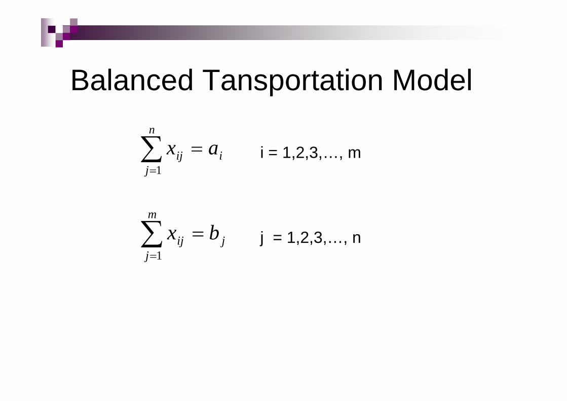
Balanced Tansportation Model
i
n
jij ax
1
j
m
jij bx
1
i = 1,2,3,…, m
j = 1,2,3,…, n

Example
Three Plants(Factories): LA, DT,NO
Two Warehouses:DV, MI
Table of cij
68102(3)NO
108100(2)DT
21580(1)LA
(2)(1)
MIDV

Example
Three Plants (Factories): LA, DT, NO
Two Warehouses: DV, MI
Table of cij
68102(3)NO
108100(2)DT
21580(1)LA
(2)(1)
MIDV

Example
Sources and Supply
Destinations and Demand
SupplySource
1200NO
1500DT
1000LA
14002300
Destination
Demand
MIDV

370014002300Demand
1200NO (3)
1500DT (2)
1000LA (1)
SupplyMI (2)DV (1)
x11
x21
x12
x22
x31 x32
80 215
100 108
102 68
Sources
Destinations
Balanced Transportation Model

14002300
1200NO (3)
1300DT (2)
1000LA (1)
MI (2)DV (1)
80 215
100 108
102 68
0 0DummyPlant
200
Unbalanced Transportation Model

40014001900
1200NO (3)
1500DT (2)
1000LA (1)
MI (2)DV (1)
80 215
100 108
102 68
0
0
Dummy
DistributionCentre
0
Unbalanced Transportation Model

Transportation – Production
5. Production and Inventory
cost from period-i to period-j
5. Transportation cost from
source-i to destination-j
4. Demand per period-j4. Demand at destination-j
3. Production capacity of
period-i
3. Supply at source-i
2. Demand period-j2. Destination-j
1. Production period-i1. Source-i
Production SystemTransportation System

The Transportation Technique
Step 1: Determine a starting feasiblesolution
Step 2: Determine an entering variablefrom the non-basic variable
If all such variables satisfy the optimalitycondition (of simplex method): STOP;
Else, GOTO Step 3

The Transportation Technique
Step 3: Determine a leaving variable(using the feasibility condition) fromamong the variables of the current basicsolution;
Find the new basic solution
RETURN TO Step 2

Determination of the StartingSolution
Northwest-corner (NWC) Rule
Least Cost Method
Vogel’s Approximation Method (VAM)

Northwest-corner
Allocate the maximum amount allowable by thesupply and demand to the variable x11 (at thenorthwest corner of the tableau)
The satisfied column (row) is then crossed out
Adjust the amounts of supply and demand for alluncrossed-out rows and columns
Do iteration until exactly one row or one columnremains uncrossed-out

NWC: Example
1015155Demand
53
252
151
4321source Supply
Destination
10 0 20 11
x12x11 x13 x14
x21
x31
x24x23x22
x32 x33 x34
12
0 14
7 9
16
20
18

NWC: Example
1015155Demand
53
252
151
4321source Supply
Destination
10 0 20 11
5
12
0 14
7 9
16
20
18

NWC: Example
1015155Demand
53
252
151
4321source Supply
Destination
10 0 20 11
5
12
0 14
7 9
16
20
18
10

NWC: Example
1015155Demand
53
252
151
4321source Supply
Destination
10 0 20 11
5
12
0 14
7 9
16
20
18
10
5

NWC: Example
1015155Demand
53
252
151
4321source Supply
Destination
10 0 20 11
5
12
0 14
7 9
16
20
18
10
5 15

NWC: Example
1015155Demand
53
252
151
4321source Supply
Destination
10 0 20 11
5
12
0 14
7 9
16
20
18
10
5 15 5

NWC: Example
1015155Demand
53
252
151
4321source Supply
Destination
10 0 20 11
5
12
0 14
7 9
16
20
18
10
5 15 5
5

1015155Demand
53
252
151
4321source Supply
Destination
10 0 20 11
5
12
0 14
7 9
16
20
18
10
5 15 5
5

Starting Solution: 5 10 + 10 0 + 5 7 +15 9 + 5 20 + 5 18 = 410
Basic Variables: x11, x12, x22, x23, x24, x34
Non-basic Variables: x13, x14, x21, x31, x32,x33

Determination of Entering VariableMethod of Multiplier
For each basic variable xij
ui : multiplier of row-i
vj : multiplier of column-j
ui + vj = cij
number of equations = m + n – 1
u1 = 0 (usually)

Determination of Entering VariableMethod of Multiplier
For each non-basic variable xpq
up : multiplier of row-p
vq : multiplier of column-q
cpq = up + vq – cpq

Determination of Entering VariableMethod of Multiplier
For each non-basic variable xpq
up : multiplier of row-p
vq : multiplier of column-q
cpq = up + vq – cpq
Maximization: xpq with most negative cpq
Minimization: xpq with the most positive cpq

1015155Demand
53
252
151
4321source Supply
Destination
10 0 20 11
5
12
0 14
7 9
16
20
18
10
5 15 5
5
Iteration #1

Basic Variable
u3 = 5
u2 = 7
u2 = 7
u2 = 7
u1 = 0
u1 = 0
v4 = 13u3 + v4 = c34 = 18x34 :
v4 = 13u2 + v4 = c24 = 20x24 :
v3 = 2u2 + v3 = c23 = 9x23 :
v2 = 0u2 + v2 = c22 = 7x22 :
v2 = 0u1 + v2 = c12 = 0x12 :
v1 = 10u1 + v1 = c11 = 10x11 :

Non-basic Variable
c33 = u3 + v3 – c33 = 5 + 2 – 16 = –9x33 :
c32 = u3 + v2– c32 = 5 + 0 – 14 = –9x32 :
c31 = u3 + v1 – c31 = 5 + 10 – 0 = 15x31 :
c21 = u2 + v1 – c21 = 7 + 10 – 12 = 5x21 :
c14 = u1 + v4 – c14 = 0 + 13 – 11 = 2x14 :
c13 = u1 + v3 – c13 = 0 + 2 – 20 = –18x13 :
x31 : entering variable

1015155Demand
53
252
151
4321source Supply
Destination
10 0 20 11
5
12
0 14
7 9
16
20
18
10
5 15 5
5
-18 2
5
15 -9 -9
x31

Determination of Leaving Variable:Loop Construction Equivalent to applying feasibility condition in
simplex method
The loop starts and end at the designated non-basic variable
Every corner of the loop should be a cell withbasic variable (except the start and the end)
Change the value of every corner alternatively(+) or (–)
Leaving variable is the one with smallest value
A tie is arbitrarily broken

1015155Demand
53
252
151
4321source Supply
Destination
10 0 20 11
5
12
0 14
7 9
16
20
18
10
5 15 5
5
x31

1015155Demand
53
252
151
4321source Supply
Destination
10 0 20 11
5
12
0 14
7 9
16
20
18
10
5 15 5
5
x31
+
– +
– +
–
x11, x22, x34 = 0 Leaving variable: x34

1015155Demand
53
252
151
4321source Supply
Destination
10 0 20 11
0
12
0 14
7 9
16
20
18
15
0 15 10
x34
5

Iteration#1
Solution: 0 10 + 15 0 + 0 7 + 15 9+ 10 20 + 5 0 = 335
Basic Variables: x11, x12, x22, x23, x24, x31
Non-basic Variables: x13, x14, x21, x32, x33,x34

1015155Demand
53
252
151
4321source Supply
Destination
10 0 20 11
0
12
0 14
7 9
16
20
18
15
0 15 10
x34
5
Iteration #2

Basic Variable
u3 = –10
u2 = 7
u2 = 7
u2 = 7
u1 = 0
u1 = 0
v1 = 10u3 + v1 = c31 = 0x31 :
v4 = 13u2 + v4 = c24 = 20x24 :
v3 = 2u2 + v3 = c23 = 9x23 :
v2 = 0u2 + v2 = c22 = 7x22 :
v2 = 0u1 + v2 = c12 = 0x12 :
v1 = 10u1 + v1 = c11 = 10x11 :

Non-basic Variable
c34 = u3 + v4 – c34 = –10 + 13 – 18 = –15x34 :
c33 = u3 + v3 – c33 = –10 + 2 – 16 = –24x33 :
c32 = u3 + v2– c32 = –10 + 0 – 14 = –24x32 :
c21 = u2 + v1 – c21 = 7 + 10 – 12 = 5x21 :
c14 = u1 + v4 – c14 = 0 + 13 – 11 = 2x14 :
c13 = u1 + v3 – c13 = 0 + 2 – 20 = –18x13 :
x21 : entering variable

1015155Demand
53
252
151
4321source Supply
Destination
10 0 20 11
0
12
0 14
7 9
16
20
18
15
0 15 10x21
5
+
+
–
–
x11, x22=0 Leaving Variable = x11

1015155Demand
53
252
151
4321source Supply
Destination
10 0 20 11
x11
12
0 14
7 9
16
20
18
15
0 15 100
5
Iteration #2

Iteration#2
Solution: 0 12 + 15 0 + 0 7 + 15 9+ 10 20 + 5 0 = 335
Basic Variables: x12, x21, x22, x23, x24, x31
Non-basic Variables: x11, x13, x14, x21, x32,x33, x34

1015155Demand
53
252
151
4321source Supply
Destination
10 0 20 11
x11
12
0 14
7 9
16
20
18
15
0 15 100
5
Iteration #3

Basic Variable
v1= 5u2 = 7u2 + v1 = c21 = 12x21 :
u3 = –5
u2 = 7
u2 = 7
u2 = 7
u1 = 0
v1 = 5u3 + v1 = c31 = 0x31 :
v4 = 13u2 + v4 = c24 = 20x24 :
v3 = 2u2 + v3 = c23 = 9x23 :
v2 = 0u2 + v2 = c22 = 7x22 :
v2 = 0u1 + v2 = c12 = 0x12 :

Non-basic Variable
c11 = u1 + v1 – c11 = 0 + 5 – 10 = –5x11 :
c34 = u3 + v4 – c34 = –5 + 13 – 18 = –10x34 :
c33 = u3 + v3 – c33 = –5 + 2 – 16 = –19x33 :
c32 = u3 + v2– c32 = –5 + 0 – 14 = –19x32 :
c14 = u1 + v4 – c14 = 0 + 13 – 11 = 2x14 :
c13 = u1 + v3 – c13 = 0 + 2 – 20 = –18x13 :
x14 : entering variable

1015155Demand
53
252
151
4321source Supply
Destination
10 0 20 11
x14
12
0 14
7 9
16
20
18
15
0 15 100
5
x24 = 0
+
+
–
–
Leaving Variable = x24

1015155Demand
53
252
151
4321source Supply
Destination
10 0 20 11
10
12
0 14
7 9
16
20
18
5
10 15 x240
5
Iteration #3

Iteration#3
Solution: 5 0 + 10 11 + 0 12 + 10 7+ 15 9 + 5 0 = 315
Basic Variables: x12, x14, x21, x22, x23, x31
Non-basic Variables: x11, x13, x24, x32, x33,x34

1015155Demand
53
252
151
4321source Supply
Destination
10 0 20 11
10
12
0 14
7 9
16
20
18
5
10 15 x240
5
Iteration #4

Basic Variable
v1 = 5u3 = –5u3 + v1 = c31 = 0x31 :
v1= 5u2 = 7u2 + v1 = c21 = 12x21 :
u1 = 0
u2 = 7
u2 = 7
u1 = 0
v4 = 11u1 + v4 = c14 = 11x14 :
v3 = 2u2 + v3 = c23 = 9x23 :
v2 = 0u2 + v2 = c22 = 7x22 :
v2 = 0u1 + v2 = c12 = 0x12 :

Non-basic Variable
c34 = u3 + v4 – c34 = –5 + 11 – 18 = –12x34 :
c33 = u3 + v3 – c33 = –5 + 2 – 16 = –19x33 :
c11 = u1 + v1 – c11 = 0 + 5 – 10 = –5x11 :
c24 = u2 + v4 – c24 = 7 + 11 – 20 = –2x24 :
c32 = u3 + v2– c32 = –5 + 0 – 14 = –19x32 :
c13 = u1 + v3 – c13 = 0 + 2 – 20 = –18x13 :
All non-basic variables are now negative = END

(Class) Assignment #3Improved Starting Solution
Elaborate the Least-Cost Method
Elaborate Vogel’s Approximation Method(VAM)
Present the elaborations

(Class) Assignment #4The Assignment Model
Elaborate the assignment model asspecific transportation model
Present the elaboration

The End
This is the end of Chapter 6A
Recommended