White PaperWhite Paper 1:14
Policy Brief 1:14
Transitioning to Electric Drive Vehicles:
Public Policy Implications of Uncertainty, Network Externalities, Tipping Points and Imperfect Markets
David L. Greene Sangsoo Park
Howard H. Baker Jr. Center for Public Policy The University of Tennessee
Changzheng Liu
National Transportation Research Center Oak Ridge National Laboratory
January 17, 2014

Baker Center Board
Cynthia BakerMedia ConsultantWashington, DC The Honorable Howard H. Baker Jr.Former Ambassador to JapanFormer United States Senator The Honorable Phil BredesenFormer Governor of Tennessee
Sam M. BrowderRetired, Harriman Oil Sarah Keeton CampbellAttorney, Williams & Connolly, LLPWashington, DC
Jimmy G. CheekChancellor, The University of Tennessee, Knoxville AB Culvahouse Jr.Attorney, O’Melveny & Myers, LLPWashington, DC
The Honorable Albert Gore Jr.Former Vice President of the United StatesFormer United States Senator Thomas GriscomCommunications ConsultantFormer Editor, Chattanooga Times Free Press
James Haslam IIChairman and Founder, Pilot CorporationThe University of Tennessee Board of Trustees Joseph E. JohnsonFormer President, University of Tennessee Fred MarcumSenior Adviser to Senator Baker The Honorable George Cranwell MontgomeryFormer Ambassador to the Sultanate of Oman Regina MurrayKnoxville, Tennessee Lee RiedingerVice Cancellor, The University of Tennessee, Knoxville
John SeigenthalerFounder, First Amendment Center, Vanderbilt University Don C. Stansberry Jr.The University of Tennessee Board of Trustees The Honorable Don SundquistFormer Governor of Tennessee William H. SwainThe University of Tennessee Development Council The Honorable Fred ThompsonFormer United States Senator Robert WallerFormer President and CEO, Mayo Clinic
Baker Center Staff
Matt MurrayDirector
Nissa Dahlin-BrownAssociate Director
Michelle Castro Development Director
Patti RebholzBusiness Manager
Elizabeth WoodyOffice Manager
Carl PierceDirector Emeritus & Senior Fellow for Baker Studies
About the Baker CenterThe Howard H. Baker Jr. Center for Public Policy is an education and research center that serves the University of Tennessee, Knoxville, and the public. The Baker Center is a nonpartisan institute devoted to education and public policy schol-arship focused onh energy and the environment, global security, and leadership and governance.
Howard H. Baker Jr. Center for Public Policy1640 Cumberland AvenueKnoxville, TN 37996-3340
The contents of this report were developed under a grant from the US Department of Education. How-ever, these contents do not necessarily represent the policy of the US Department of Education, and you should not assume endorsement by the federal government. Findings and opinions conveyed herein are those of the authors only and do not necessarily represent an official position of the Howard H. Baker Jr. Center for Public Policy or the University of Tennessee.
Patrick ButlerCEO, Assoc. Public Television Stations
Baker Center Board
Cynthia BakerMedia ConsultantWashington, DC The Honorable Howard H. Baker Jr.Former Ambassador to JapanFormer United States Senator The Honorable Phil BredesenFormer Governor of Tennessee
Sam M. BrowderRetired, Harriman Oil Sarah Keeton CampbellAttorney, Williams & Connolly, LLPWashington, DC
Jimmy G. CheekChancellor, The University of Tennessee, Knoxville AB Culvahouse Jr.Attorney, O’Melveny & Myers, LLPWashington, DC
The Honorable Albert Gore Jr.Former Vice President of the United StatesFormer United States Senator Thomas GriscomCommunications ConsultantFormer Editor, Chattanooga Times Free Press
James Haslam IIChairman and Founder, Pilot CorporationThe University of Tennessee Board of Trustees Joseph E. JohnsonFormer President, University of Tennessee Fred MarcumSenior Adviser to Senator Baker The Honorable George Cranwell MontgomeryFormer Ambassador to the Sultanate of Oman Regina MurrayKnoxville, Tennessee Lee RiedingerVice Cancellor, The University of Tennessee, Knoxville
John SeigenthalerFounder, First Amendment Center, Vanderbilt University Don C. Stansberry Jr.The University of Tennessee Board of Trustees The Honorable Don SundquistFormer Governor of Tennessee William H. SwainThe University of Tennessee Development Council The Honorable Fred ThompsonFormer United States Senator Robert WallerFormer President and CEO, Mayo Clinic
Baker Center Staff
Matt MurrayDirector
Nissa Dahlin-BrownAssociate Director
Michelle Castro Development Director
Patti RebholzBusiness Manager
Elizabeth WoodyOffice Manager
Carl PierceDirector Emeritus & Senior Fellow for Baker Studies
About the Baker CenterThe Howard H. Baker Jr. Center for Public Policy is an education and research center that serves the University of Tennessee, Knoxville, and the public. The Baker Center is a nonpartisan institute devoted to education and public policy schol-arship focused onh energy and the environment, global security, and leadership and governance.
Howard H. Baker Jr. Center for Public Policy1640 Cumberland AvenueKnoxville, TN 37996-3340
The contents of this report were developed under a grant from the US Department of Education. How-ever, these contents do not necessarily represent the policy of the US Department of Education, and you should not assume endorsement by the federal government. Findings and opinions conveyed herein are those of the authors only and do not necessarily represent an official position of the Howard H. Baker Jr. Center for Public Policy or the University of Tennessee.
The Howard H. Baker Jr. Center for Public Policy is a non-partisan institute at the University of Tennessee, Knoxville, dedicated to education, research and civil discussion of policy issues. We are proud to present this White Paper series to help promote discussion and dialogue on matters of policy that are of importance to the research community, policymakers and the nation at large. Each White Paper is intended to take on its own unique flavor, reflecting the specific research question at hand and the way in which researchers have sought to address it. We hope to present provocative and impactful research from a wide array of policymakers, scholars and disciplines that is rooted in the values and ideals of Senator Baker as demonstrated by his long and illustrious career in public service. In the end our goal is a well-informed electorate and sound public policy that will advance the wellbeing of the state and the nation.
Matthew N. Murray, PhD
Director
Welcome to the new White Paper series of the Howard H. Baker Jr. Center for Public Policy. An informed electorate is essential for our Republic to function effectively. Therefore, we have created this series to promote ongoing research and encourage discussion about issues of concern to everyone. These White Papers will seek to explore current issues and offer research results, literature reviews, and suggestions for further research, all of which can be used to inform citizens and decision-making at all levels of society. It is my hope that you will find this series informative and thought-provoking and we welcome your comments.
Howard H. Baker, Jr.

The Howard H. Baker Center for Public Policy The Howard H. Baker Center for Public Policy I
Baker Center Board
Cynthia BakerMedia ConsultantWashington, DC The Honorable Howard H. Baker Jr.Former Ambassador to JapanFormer United States Senator The Honorable Phil BredesenFormer Governor of Tennessee
Sam M. BrowderRetired, Harriman Oil Sarah Keeton CampbellAttorney, Williams & Connolly, LLPWashington, DC
Jimmy G. CheekChancellor, The University of Tennessee, Knoxville AB Culvahouse Jr.Attorney, O’Melveny & Myers, LLPWashington, DC
The Honorable Albert Gore Jr.Former Vice President of the United StatesFormer United States Senator Thomas GriscomCommunications ConsultantFormer Editor, Chattanooga Times Free Press
James Haslam IIChairman and Founder, Pilot CorporationThe University of Tennessee Board of Trustees Joseph E. JohnsonFormer President, University of Tennessee Fred MarcumSenior Adviser to Senator Baker The Honorable George Cranwell MontgomeryFormer Ambassador to the Sultanate of Oman Regina MurrayKnoxville, Tennessee Lee RiedingerVice Cancellor, The University of Tennessee, Knoxville
John SeigenthalerFounder, First Amendment Center, Vanderbilt University Don C. Stansberry Jr.The University of Tennessee Board of Trustees The Honorable Don SundquistFormer Governor of Tennessee William H. SwainThe University of Tennessee Development Council The Honorable Fred ThompsonFormer United States Senator Robert WallerFormer President and CEO, Mayo Clinic
Baker Center Staff
Matt MurrayDirector
Nissa Dahlin-BrownAssociate Director
Michelle Castro Development Director
Patti RebholzBusiness Manager
Elizabeth WoodyOffice Manager
Carl PierceDirector Emeritus & Senior Fellow for Baker Studies
About the Baker CenterThe Howard H. Baker Jr. Center for Public Policy is an education and research center that serves the University of Tennessee, Knoxville, and the public. The Baker Center is a nonpartisan institute devoted to education and public policy schol-arship focused onh energy and the environment, global security, and leadership and governance.
Howard H. Baker Jr. Center for Public Policy1640 Cumberland AvenueKnoxville, TN 37996-3340
The contents of this report were developed under a grant from the US Department of Education. How-ever, these contents do not necessarily represent the policy of the US Department of Education, and you should not assume endorsement by the federal government. Findings and opinions conveyed herein are those of the authors only and do not necessarily represent an official position of the Howard H. Baker Jr. Center for Public Policy or the University of Tennessee.
The Howard H. Baker Jr. Center for Public Policy is a non-partisan institute at the University of Tennessee, Knoxville, dedicated to education, research and civil discussion of policy issues. We are proud to present this White Paper series to help promote discussion and dialogue on matters of policy that are of importance to the research community, policymakers and the nation at large. Each White Paper is intended to take on its own unique flavor, reflecting the specific research question at hand and the way in which researchers have sought to address it. We hope to present provocative and impactful research from a wide array of policymakers, scholars and disciplines that is rooted in the values and ideals of Senator Baker as demonstrated by his long and illustrious career in public service. In the end our goal is a well-informed electorate and sound public policy that will advance the wellbeing of the state and the nation.
Matthew N. Murray, PhD
Director
Welcome to the new White Paper series of the Howard H. Baker Jr. Center for Public Policy. An informed electorate is essential for our Republic to function effectively. Therefore, we have created this series to promote ongoing research and encourage discussion about issues of concern to everyone. These White Papers will seek to explore current issues and offer research results, literature reviews, and suggestions for further research, all of which can be used to inform citizens and decision-making at all levels of society. It is my hope that you will find this series informative and thought-provoking and we welcome your comments.
Howard H. Baker, Jr.

The Howard H. Baker Center for Public PolicyII
The Baker Center White Paper series are issued by the Howard H. Baker Jr. Center for Public Policyat the University of Tennessee, Knoxville. These White Papers are designed to inform and promotediscussion and dialogue on matters of public policy. The opinions and statements made in these papersare those of the authors and do not necessarily represent the views of the staff of the Baker Center orthe University of Tennessee. Copyright 2014 by THE UNIVERSITY OF TENNESSEE.

The Howard H. Baker Center for Public Policy The Howard H. Baker Center for Public Policy III
Start Page numbering on this page as page i
Acknowledgments
The authors thank the International Council for Clean Transportation for the opportunity to carry out this research. We thank Anup Bandivadekar, Chuck Shulock, John German and Alan Lloyd for their many insights, observations and suggestions for improving the study and the report. We thank colleagues from industry, government, NGOs and academia who listened to briefings on our work, asked challenging questions and provided peer review. Any remaining errors or omissions in this report are the responsibility of the authors.

The Howard H. Baker Center for Public PolicyIV
page ii
Abstract
This report builds on a previous Baker Center analysis of the transition to electric drive light-‐duty vehicles in California and the Section 177 states that have adopted California’s Zero Emission Vehicle standards.1 That study estimated the costs and benefits of a transition to electric drive vehicles under six alternative scenarios using the same model and technology and market assumptions from a recent National Research Council study. It concluded that, given the NRC assumptions, benefits would like exceed costs by roughly an order of magnitude. Targeted, temporary transitions policies would be required however; internalizing external costs alone would likely be inadequate to accomplish the transition. This study estimates the effects of the timing and intensity of policies and adds uncertainty about technological progress to the previous study’s analysis of uncertainty about the market’s response. The analyses presented in this report are based on Scenario 2 of the previous report, in which the ZEV standards are enforced through 2025 and continued at the 2025 level through 2030 and then ended. The rest of the U.S. is assumed to follow California’s lead, adopting similar policies and deploying refueling infrastructure but five years later than California and the Section 177 states. The new model runs indicate that, given the assumptions of Scenario 2, starting the ZEV standards 5 years earlier or doubling their intensity increases upfront costs but increases benefits by a greater amount. Similarly, delaying the ZEV mandate is estimated to reduce upfront costs but cause an even greater reduction in the present value of benefits. Network effects and other positive feedbacks were measured to illustrate the dynamics of the transition. The impacts of mandates or subsidies was strongly dependent on their timing and context. The simulations again showed the important synergies between California and U.S. transition policies. The effects of technological and market uncertainty were simulated assuming policies that forced the achievement of the market shares of PHEVs, BEVs and FCVs of Scenario 2. This assumption should overestimate the costs of the transition relative to policies that adapt to circumstances. Nevertheless, the frequency of negative net present values was less than 10%.
1 http://bakercenter.utk.edu/wp-‐content/uploads/2013/06/Transition-‐to-‐Electric-‐Drive-‐2013-‐report.FINAL_.pdf

The Howard H. Baker Center for Public Policy The Howard H. Baker Center for Public Policy 1
Table of Contents
ADJUST THESE PAGES as needed
I. Introduction……………………………………………………………………………………………………………2
II. The Economics of Large-‐Scale Energy Transition………….……………………………..………….4
III. Modeling the Transition to Electric Drive Vehicles………………………………………………..11
IV. Network External Benefits and Policy Feedback Effects………………………………………..28
V. Timing and Intensity of Policies…………………………………………………………………………….42
VI. Uncertainty and Outcomes…………………………………………………………………………………..46
VII. Inferences for Policymaking………………………………………………………………………………….58
VIII. References……………………………………………………………………………………………………………61
Appendix………………………………………………………………………………………………………………
67

The Howard H. Baker Center for Public Policy2
Transitioning to Electric Drive Vehicles: Public Policy Implications of Uncertainty, Network Externalities, Tipping Points and Imperfect
Markets
David L. Greene Sangsoo Park Changzheng Liu
“Without question a radical transformation of the present energy system will be
required over the coming decades.” (p. xiii)
“An effective transformation requires immediate action.” (p. xv)
“In all (sustainable, ed.) pathways conventional oil is essentially phased out shortly after 2050.” (p. 51)
(IIASA, Global Energy Assessment, 2012)
I. Introduction
The world’s transportation system depends on fossil petroleum for 95% of the energy it uses and transportation produces about 20% of anthropogenic greenhouse gas emissions (IEA, 2012). Achieving both energy security and climate protection will likely require a transition from a petroleum-‐powered transportation system to one that relies on a combination of electricity, hydrogen and biofuels (NRC, 2013), all produced with very low lifecycle greenhouse gas emissions. How to accomplish such a large-‐scale energy transition efficiently and effectively is an enormous challenge for public policy.
This report is a sequel to the report, “Analyzing the Transition to Electric Drive in California”, in which the LAVE-‐Trans model was used to analyze six scenarios of the transition to electric drive vehicles in California.2 This report follows up that analysis by expanding on the theory of economically efficient, large-‐scale energy transitions and exploring four issues raised by but not addressed in the earlier report:
1. Quantifying the effects of network external benefits and other positive feedbacks over time;
2. Measuring the effect of the timing of transition policies on the transition’s net present value;
2 Throughout this report the term “electric drive” includes grid connected (battery electric and plug-‐in hybrid) vehicles and fuel cell electric vehicles powered by hydrogen.

The Howard H. Baker Center for Public Policy The Howard H. Baker Center for Public Policy 3
3. Measuring the effect of the intensity of transition policies on the transition’s net present value;
4. Quantifying the effects of uncertainties about technological progress and market behavior on the net present value of the transition.
Section II addresses the economic efficiency of a transition to an alternative energy system within the context of cost/benefit analysis under deep uncertainty. The length of time required for an energy transition, the deep uncertainty about technological change and the market’s response to new technologies, the strong positive feedback effects that create tipping points and the need to address both energy security and greenhouse gas mitigation make the transition problem different from regulating or pricing externalities. In addition, the problems to be solved, such as monopoly power in world oil markets or achieving a sustainable energy system, are not externalities. Previous modeling of the transition to alternative vehicles and fuels has indicated that internalizing external costs alone would likely be insufficient to induce a transition (e.g., NRC, 2013; Greene et al., 2013).
It is argued that the appropriate economic framework is cost/benefit analysis under deep uncertainty. It is a search for futures that substantially improve social welfare, recognizing that the alternative futures are uncertain and likely to be path-‐dependent. The framework proposed is in the spirit of Coase’s (1960) analysis of the general problem of social costs.3
“A better approach would seem to be to start our analysis with a situation approximating that which actually exists, to examine the effects of a proposed policy change and to attempt to decide whether the new situation would be, in total, better or worse than the original one.” (Coase, 1960, p. 43)
Although Coase was arguing for the allocation of property rights as a more general solution to the problem of social costs than externality taxes, the reasoning applies equally well to the problem of an energy transition. However, instead of comparing the current situation to a hypothetical alternative the large-‐scale energy transition problem requires comparing alternative futures.
Section III presents a brief review of the LAVE-‐Trans model whose simulation results will be used in sections IV, V and VI to illustrate three important aspects of the transition problem. Illustrating the network external benefits and other positive feedbacks that create tipping points is the subject of Section IV. Section V explores how the timing and intensity of policy
3 The authors are grateful to Professor Severin Borenstein whose observations on the death of Coase (“Learning and Forgetting the Wisdom of Coase”, September 9,2013) pointed us to Coase’s seminal article. http://energyathaas.wordpress.com/2013/09/09/learning-‐and-‐forgetting-‐the-‐wisdom-‐of-‐coase/?utm_source=Blog+Sep+9%2C+2013&utm_campaign=blog35&utm_medium=email
The Howard H. Baker Center for Public Policy4
actions affect the costs and benefits of the transition. Section VI addresses the important role of uncertainty by quantifying uncertainty via Monte Carlo simulation and then by estimating how perceptions of risk may affect decision making.
II. The Economics of Large-‐Scale Energy Transition
There are several important factors that make the economics of a large-‐scale energy transition different from other energy and environmental policy challenges.
A major energy transition takes decades and its impacts will last for decades, at least (Gallagher, et al., 2012). Over periods of 50 years or so, the difference between social and private discount rates can make an enormous difference in the net present value of the transition. Because of the time scale, the question of intergenerational equity is intrinsic.
A self-‐sustaining transition is likely to require technological progress which is inherently uncertain, as are future economic conditions. Even if the transition does not require technological progress, technological change is virtually certain to occur.
The primary motivation for the transition is to secure public goods: environmental protection, energy security and sustainability (Greene, 2010).
Not all of the social costs being addressed are externalities. Monopoly power in world oil markets, for example, is the critical market failure for the U.S. transportation sector’s energy security problem (Greene et al., 2013b; NRC, 2009, pp. 233-‐236). Internalizing external costs is unlikely to be an adequate or efficient transition policy.
There are other important market shortcomings, especially the tendency of markets to undervalue energy efficiency (i.e., the energy paradox: e.g., Jaffe and Stavins, 1994; Sanstad and Howarth, 1994; Allcott and Greenstone, 2012), that create inefficiencies in energy markets (Greene, 2011c; Greene et al., 2013c).
The transition creates external benefits that are difficult or impossible for private agents to capture and therefore lead to market inefficiencies:
Direct network external benefits (Farrell and Klemperer, 2007): e.g., vehicle purchases by innovators and early adopters reduce the risk-‐aversion of the majority of consumers (Jaffe and Stavins, 1994; Katz and Shapiro, 1986).
Increased vehicle sales lead to greater diversity of choices and thus increased consumers’ surplus (opposed by the need for scale economies).

The Howard H. Baker Center for Public Policy The Howard H. Baker Center for Public Policy 5
There are also strong network effects that by themselves do not lead to market inefficiencies but do create strong positive feedbacks (Page and Lopatka, 1999).
Indirect network external benefits: e.g., deploying refueling or recharging infrastructure increases the value of electric drive vehicles to their owners and potential purchasers.
Pecuniary externalities are created by learning-‐by-‐doing within firms as well as spillovers in vehicle manufacturing and energy supply, and by scale economies in vehicle manufacturing and fuel supply.
The positive feedback effects of the transition process create tipping points and multiple equilibria, the timing and necessary conditions for which are profoundly uncertain.
Indirect network externalities and pecuniary externalities do not, by themselves, necessarily lead to inefficient market solutions (Katz and Shapiro, 1994). However, especially in the early stages of the transition, the vehicle and fuel markets are likely to be imperfectly competitive. Sparse, early fuel markets will almost certainly include spatial monopolies, motor fuel supply in the U.S. is oligopolistic, and motor vehicle manufacturing in general is either competitive for all practical purposes or oligopolistic.4 The combination of imperfect competition and indirect and pecuniary network externalities can lead to inefficient market outcomes.
The combination of all these conditions requires a public policy strategy appropriate to the nature of the problem. Internalizing negative externalities alone is not likely to be effective or efficient. Internalizing negative external costs will not address network external benefits. These would also have to be priced or captured by private agents. Second, the social costs and benefits that are not externalities, namely oil dependence and sustainability, would not be adequately corrected. Third, internalizing external costs would not address the important difference between societal and market discount rates over a period on the order of half a century. And finally, the combination of strong positive feedbacks that create tipping points and deep uncertainties about future technological and market conditions imply that transition policies should be adaptable and temporary, to be changed when new information is acquired and phased out once the transition has been established.
There are also important negative feedback effects. Early in the transition, as more alternative energy vehicles are sold, the innovator and early adopter market segment not only tends to become saturated but progressively loses interest in what is no longer a truly novel technology. Their willingness to pay a premium for a novel technology decreases as cumulative sales increases. The second effect is not so
4 The correct economic terminology is “monopolistically competitive”, which describes markets in which firms can differentiate their products from their competitors’, at least temporarily, but in which in the long run products tend to sell at long-‐run average cost.

The Howard H. Baker Center for Public Policy6
much a negative feedback effect as a saturation of the consumers who have a natural preference for one vehicle technology over another. In model typically used to predict consumers’ choices among discrete alternatives, commodities are assumed to have “unobserved” attributes that are important to consumers but not explicitly included in the choice model’s calculations. These are assumed to vary randomly across the population of consumers. As sales of one technology increase, additional sales become increasingly difficult because it is necessary to win over consumers with an increasingly large unobserved preference for other technologies. Thus, the advantage of the technology in question has to be more and more compelling to continue capturing additional customers.
Decisions about long-‐term transitions must be made despite “deep uncertainty” about future technology and markets. In such situations robust and adaptive strategies are generally superior to fixed strategies based on a best guess of what is optimal (Lempert et al., 2006). The strong positive feedbacks of the transition process create “tipping points” whose preconditions and timing are generally uncertain (Cabral, 1990; Lemoine and Traeger, 2012). Decision makers and the public are likely to be risk-‐averse (Arrow and Lind, 1970) or loss-‐averse (Tversky and Kahneman, 1992). All of this underlines the importance of improving knowledge and understanding of the transition process in order to reduce uncertainty and increase the likelihood that the decisions taken will be beneficial.
Net Present Value
An appropriate metric for evaluating transition policies is the present value of future economic welfare (Lemoine and Traeger, 2012). The net present value (NPV) of an energy transition can be measured by the discounted value of the stream of changes in costs and benefits relative to a reference or base case projection. For simplicity, consider two types of benefits, private (BP) and public (BU) and two types of costs, subsidies to fuels (CF) and vehicles (CV). The benefit and cost functions may vary over the time interval of interest (t=0, T) and both are a function of an n×t matrix of state and policy variables (Xt) whose time dimension increases over time as t→T. Costs and benefits are also functions of a vector of parameters, bt, that may change with time and whose values are for now assumed to be known but that in reality are uncertain. The variables in the matrix account for all the important interactions in the system, including policies, vehicle sales and stocks, fuel sales, prices, etc. Discounting could be over discrete or continuous time; for consistency with the LAVE-‐Trans model discrete time is used, with the discount rate of 0 ≤ r ≤ 1.
Equation 1
!"! =1
1+ ! ! !!" !! ,!! + !!" !! ,!! − !!" !! ,!! − !!" !! ,!!!
!!!
Where Xt is a matrix and bt is a vector:

The Howard H. Baker Center for Public Policy The Howard H. Baker Center for Public Policy 7
!! =!!! ⋯ !!"⋮ ⋱ ⋮!!" ⋯ !!!
!! = !!! , !!! ,… !!"
A transition that maximizes net present value must satisfy the following first order condition for each policy variable, !!∗ , namely that marginal cost equal marginal benefits:
Equation 2
max!!∗
11+ ! ! !!" !! ,!! + !!" !! ,!! − !!" !! ,!! − !!" !! ,!!
!
!!!
1
1+ ! !!!!" !! ,!!
!!!∗+!!!" !! ,!!
!!!∗−!!!" !! ,!!
!!!∗−!!!" !! ,!!
!!!∗= 0
!
!!!
11+ ! !
!!!" !! ,!!!!!∗
+!!!" !! ,!!
!!!∗=
11+ ! !
!!!" !! ,!!!!!∗
+!!!" !! ,!!
!!!∗
!
!!!
!
!!!
The left hand side of the first order condition represents the total discounted marginal benefit of the policy variable !!∗ and the right hand side is the total discounted marginal cost of !!∗.5
The effect of a marginal change in policy, e.g. a vehicle or fuel subsidy, on the NPV of a transition is given by the derivative of NPV with respect to that variable. It is clear from equation 2 that first order conditions for maximizing NPV require that each variable be chosen such that marginal total benefits equal marginal total costs in each year. The benefit and cost functions in any given year depend on previous values of the policy variables.
Consider a small change in a policy variable in year t-‐m (xit-‐m).6
5 To insure an optimum, the second order condition of !!∗ must also be satisfied:
!1
(1 + %)' ()2+,'(-', /')
)0'∗2+)2+2'(-', /')
)0'∗2−)245'(-', /')
)0'∗2−)246'(-', /')
)0'∗27 ˂ 0
;
'=0
However, the existence of tipping points implies discontinuities in the NPV function and multiple optima. 6 The change is assumed to be small enough not to cause a tipping point (discussed below).
The Howard H. Baker Center for Public Policy8
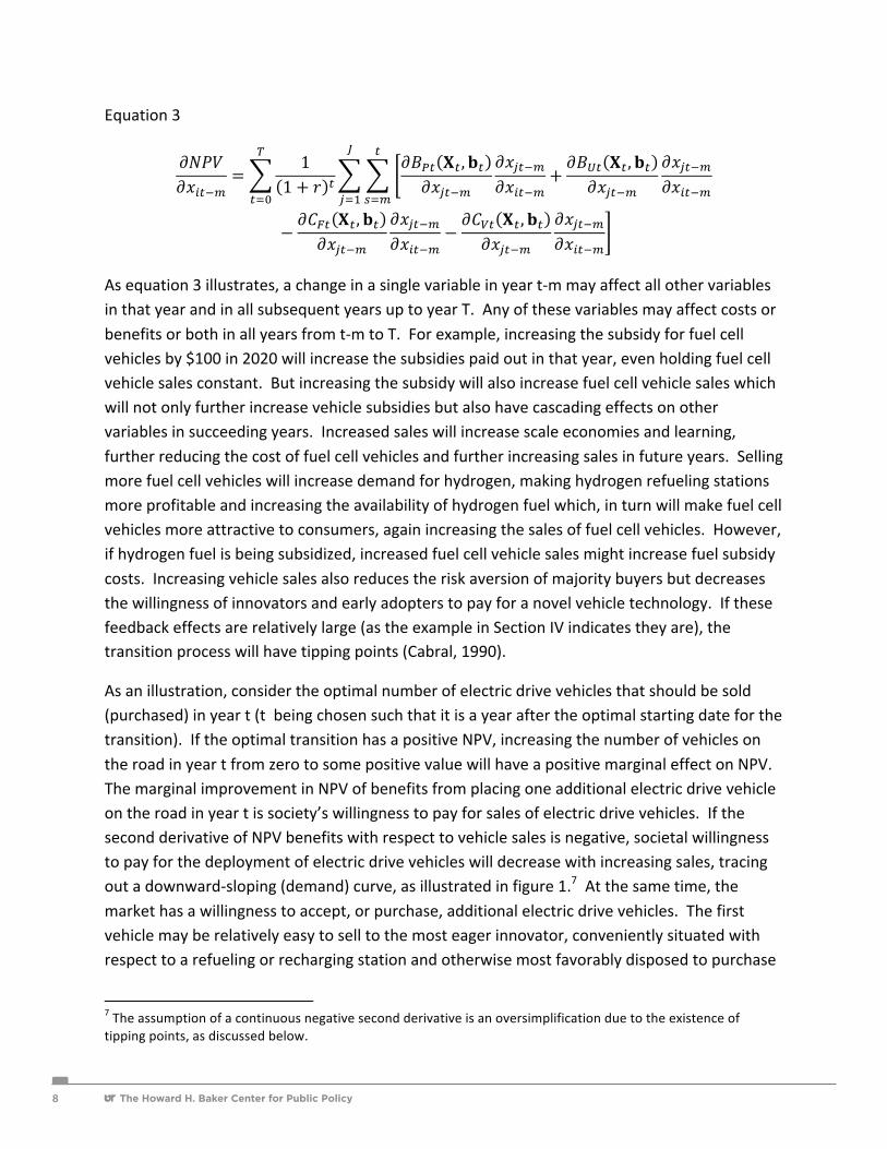
Equation 3
!"#$!!!"!!
=1
1+ ! !!!!" !! ,!!!!!"!!
!!!"!!!!!"!!
+!!!" !! ,!!!!!"!!
!!!"!!!"!"!!
!
!!!
!
!!!
!
!!!
−!!!" !! ,!!!!!"!!
!!!"!!!!!"!!
−!!!" !! ,!!!!!"!!
!!!"!!!!!"!!
As equation 3 illustrates, a change in a single variable in year t-‐m may affect all other variables in that year and in all subsequent years up to year T. Any of these variables may affect costs or benefits or both in all years from t-‐m to T. For example, increasing the subsidy for fuel cell vehicles by $100 in 2020 will increase the subsidies paid out in that year, even holding fuel cell vehicle sales constant. But increasing the subsidy will also increase fuel cell vehicle sales which will not only further increase vehicle subsidies but also have cascading effects on other variables in succeeding years. Increased sales will increase scale economies and learning, further reducing the cost of fuel cell vehicles and further increasing sales in future years. Selling more fuel cell vehicles will increase demand for hydrogen, making hydrogen refueling stations more profitable and increasing the availability of hydrogen fuel which, in turn will make fuel cell vehicles more attractive to consumers, again increasing the sales of fuel cell vehicles. However, if hydrogen fuel is being subsidized, increased fuel cell vehicle sales might increase fuel subsidy costs. Increasing vehicle sales also reduces the risk aversion of majority buyers but decreases the willingness of innovators and early adopters to pay for a novel vehicle technology. If these feedback effects are relatively large (as the example in Section IV indicates they are), the transition process will have tipping points (Cabral, 1990).
As an illustration, consider the optimal number of electric drive vehicles that should be sold (purchased) in year t (t being chosen such that it is a year after the optimal starting date for the transition). If the optimal transition has a positive NPV, increasing the number of vehicles on the road in year t from zero to some positive value will have a positive marginal effect on NPV. The marginal improvement in NPV of benefits from placing one additional electric drive vehicle on the road in year t is society’s willingness to pay for sales of electric drive vehicles. If the second derivative of NPV benefits with respect to vehicle sales is negative, societal willingness to pay for the deployment of electric drive vehicles will decrease with increasing sales, tracing out a downward-‐sloping (demand) curve, as illustrated in figure 1.7 At the same time, the market has a willingness to accept, or purchase, additional electric drive vehicles. The first vehicle may be relatively easy to sell to the most eager innovator, conveniently situated with respect to a refueling or recharging station and otherwise most favorably disposed to purchase
7 The assumption of a continuous negative second derivative is an oversimplification due to the existence of tipping points, as discussed below.

The Howard H. Baker Center for Public Policy The Howard H. Baker Center for Public Policy 9
an electric drive vehicle. The second vehicle will be somewhat more difficult to sell, and so on. The cost to society of selling these vehicles is the subsidy that must be paid to achieve the given sales level.8 The increasing cost or subsidy required to insure the sale of each additional electric drive vehicle traces out the market’s willingness-‐to-‐accept (or supply) function for electric drive vehicles. At the intersection of the two curves, marginal benefits due to selling more electric drive vehicles equals the marginal subsidy cost, thereby maximizing social surplus.
Figure 1. Illustration of an Efficient Level of Electric Drive Vehicle Sales in Year t in the Absence of Tipping Points
Tipping Points
Tipping points occur when gradually changing one or more control variables leads to a discontinuous change in the state of a system (e.g., Lamberson and Page, 2012). The feedback effects described above, including network external benefits (direct and indirect, pecuniary and non-‐pecuniary), can cause a sudden change in outcomes. Tipping points were observed in the first phase of this study when the addition of a single hydrogen refueling station outside of California and the Section 177 states caused the market to flip from dominance by internal combustion engine vehicles to hydrogen fuel cell vehicles by 2050 (Greene, et al., 2013a). Similarly, very small changes in the subsidy to one vehicle technology in a single year were seen to cause a transformation of the market. In Section IV, the LAVE-‐Trans model is used to estimate the magnitude of network external benefits and other positive feedbacks. The positive feedback effects turn out to be strong which, as Cabral (1990) has shown, will cause tipping points in the technology adoption functions. Mathematical models may be more sensitive to small changes than real world systems, yet real world tipping points exist in environmental, economic and social systems (Lamberson and Page, 2012). The existence of tipping points in the transition to low-‐carbon vehicles and fuels in particular has been 8 Subsidies may be for vehicles or fuels or infrastructure. The question of the optimal allocation of subsidies is overlooked here for simplicity.

The Howard H. Baker Center for Public Policy10
recognized previously (Struben and Sterman, 2008), as has the tendency for positive feedbacks to create path dependency (Köhler et al., 2006; Arthur, 1990). The degree of path dependence will vary from one technology to another and it will generally be possible to change direction, at some cost, when information is gained through experience. The specific conditions for future tipping points are generally highly uncertain (Lemoine and Traeger, 2012) which poses difficult problems for decision making. Because tipping points can dramatically change social welfare, reducing the uncertainty through research and analysis can have great value.
Uncertainty
The process of energy transition is characterized by “deep” uncertainty. Energy transitions require decades and future changes technology, economic conditions, consumers’ preferences and public policies are inherently uncertain. In addition, many of the factors that are important to the transition process are not well understood today (e.g., the numbers of innovators and their willingness to pay for novel vehicle technologies, the intensity and persistence of risk aversion of the majority of consumers, the cost of limited fuel availability, the cost of limited range and long recharging times, etc.). This not only makes the NPV of the transition uncertain but the impacts of policy actions will be uncertain, as well. When the uncertainty about the system’s behavior is combined with the existence of tipping points, the result is deep uncertainty.
One way to describe this uncertainty is to represent every parameter in the vector bt, parameters describing technology as well as consumers’ preferences, by a different probability distribution (g1(b1t), g2(b2t), etc.). The NPV thereby becomes a random variable but with a complex probability distribution that includes tipping points:
Equation 4
!"# = 1
1+ ! ! !!" !! ,!! + !!" !! ,!! − !!" !! ,!!!
!!!
− !!" !! ,!! !! !!! !! !!! …!! !!"
In section VI this probability distribution, over time, is estimated by Monte Carlo simulation using a single-‐region U.S. version of the LAVE-‐Trans model.

The Howard H. Baker Center for Public Policy The Howard H. Baker Center for Public Policy 11
III. Modeling the Transition to Electric Drive Vehicles
The analyses of transitions to electric drive vehicles presented in this report were carried out using the Light-‐duty Alternative Vehicles and Energy Transitions (LAVE-‐Trans) model. Readers who are familiar with the LAVE-‐Trans model as described in the first report on this project (Greene et al., 2013a) may prefer to skip this section. The LAVE-‐Trans model was also used in the National Research Council’s study, Transitions to Alternative Vehicles and Fuels (NRC, 2013, Appendix H ). The LAVE-‐Trans model represents consumers’ choices among vehicle technologies, the effects of scale, learning and technological change on the costs and performance of vehicles, and the supply of energy for vehicles. Consumers’ choices are estimated using a representative consumer, nested multinomial logit model (e.g., Greene, 2001; Greene, Leiby and Bowman, 2007; Struben and Sterman, 2008). There is a great deal of uncertainty about the best values for many of the parameters that determine consumers’ choices and firms’ decisions, in addition to the uncertainty about future technological progress. The method of deriving key choice model parameter from basic assumptions pioneered by Donndenlinger and Cook (1997) and adapted to vehicle choice modeling by Greene (2001) was used to calibrate the LAVE-‐Trans model’s vehicle choice equations. In the face of great uncertainty this method has the advantage of insuring at least the plausibility of key estimates as well as providing a direct link between assumptions and model behavior. In general, the parameter values of the NRC (2013) study are used in all scenarios in this study.
The LAVE-‐Trans model includes several feedback loops through which adoption of alternative vehicles and fuels generates network external benefits that drive down costs and increase the acceptability to consumers of the novel technologies and fuels. For example, in the LAVE-‐Trans model, consumers are divided into innovators/early-‐adopters and the majority. As vehicles are sold, the risk aversion of the majority is diminished while the preference for novelty of the innovators/early-‐adopters is likewise eroded. As more fuel cell vehicles are sold, more refueling stations are built. As more stations are built, the attractiveness of hydrogen fuel cell vehicles to consumers increases. As more vehicles are sold, costs approach long-‐run, high volume levels through the benefits of scale economies and learning-‐by-‐doing (e.g., Weiss et al, 2012). At present, quantitative knowledge about many of these relationships is weak. The approach taken in LAVE-‐Trans is to use best available data, informed by judgment, and to seek to narrow uncertainties over time as knowledge grows.
At the heart of the model are consumers’ choices among alternative drive-‐train technologies. These choices are influenced by the prices and attributes of the drive-‐train technologies, but also by their familiarity and the availability of fuel for them. These factors (Xij) together with consumers’ preferences (represented by factor weights (αj) determine a quantitative index of utility, Ui, for each alternative (i). A key factor is the price of the vehicle, Pi. Multiplying and

The Howard H. Baker Center for Public Policy12
dividing the utility index function by the coefficient of vehicle price (β) converts each factor’s weight to a measure of present value dollars. The term in brackets in equation 5 is a measure of the general value (or cost) of alternative i. The value of each component in the utility function can therefore be measured in dollars, which allows estimation of the dollar value of changes in fuel availability, diversity of choice, majority risk aversion, etc.
Equation 5
As the prices and attributes of new vehicles change, vehicle sales may increase or decrease. The nested logit model allows the effects of these changes on consumers’ satisfaction (consumers’ surplus) to be measured in dollars. In the nested model, utilities are aggregated over the nesting levels to arrive at a general utility of purchasing or not purchasing a car. The change in consumers’ surplus from the Base Case (U0) to a policy case (U1) can then be calculated using equation 6, due to Small and Rosen (1981).
Equation 6
∆!" = −1!∗ !" !!!"#
!+ !!!"!!"#
!− !" !!!"#
!+ !!!"!!"#
!
Figure 2 illustrates the relationships between the major components of the model. The areas where exogenous inputs enter the model are shown as blue boxes. A relatively large amount of exogenous information is required to carry out a model run. Baseline projections of vehicle sales and energy prices are required to 2050. Technical attributes of advanced technology vehicles, including fuel consumption per km, on-‐board energy storage and retail price equivalent at full scale and learning, must be specified for current and certain future years. Parameters that determine consumers’ willingness to pay for vehicles and their attributes must also be provided. The model translates these into coefficients for the vehicle choice model. Capital and operating costs of both electric and hydrogen infrastructure must also be provided. The LAVE-‐Trans model has been implemented as an Excel spreadsheet model comprised of 27 worksheets.
⎟⎟⎠
⎞⎜⎜⎝
⎛+=+= ∑∑
==iij
n
j
jn
jiijji PXPXU
11 β
αββα

The Howard H. Baker Center for Public Policy The Howard H. Baker Center for Public Policy 13
Figure 2. Diagrammatic Representation of the LAVE-‐Trans Model.
The LAVE-‐Trans model was calibrated to the 2011 Annual Energy Outlook Reference (AEO) Case projections of vehicle sales, vehicle use, energy use and energy prices (EIA, 2011). Given a starting sales projection, the Vehicle Choice model first estimates any changes to consumers’ vehicle purchase decisions, then estimates the shares of ICE, HEV, PHEV, BEV and FCV technologies for passenger cars and light trucks for both the Innovator/Early-‐adopter and Majority market segments. Sales are passed to the Vehicle Stock worksheet which retires vehicles as they age and keeps track of the number of vehicles of each technology type by model year, for every forecast year using the U.S. Department of Transportation’s scrappage functions (NHTSA, 2006). Vehicle kilometers by age and vehicle type depend on fuel prices and energy efficiency, are calculated in the Vehicle Use worksheet and are also based on NHTSA (2006). In the Energy Use worksheet energy use is calculated for all but PHEVs by multiplying vehicle kilometers by number of vehicles and by energy consumption per kilometer. PHEV use of electricity and gasoline depends on specified shares of total miles traveled powered by gasoline and electricity and is calculated in a separate worksheet. Well-‐to-‐wheel greenhouse gas, NOx, HC, and PM10 emissions factors are applied in other worksheets to calculate total emissions.

The Howard H. Baker Center for Public Policy14
The structure of the nested multinomial logit choice model is shown in figure 3. Consumers evaluate the three kinds of drive-‐trains that include internal combustion engines (ICE, HEV, PHEV) and compare the internal combustion alternatives with the battery electric and fuel cell options. At the lowest level in the diagram, choices are most price sensitive, reflecting the greater similarity (or degree of substitutability) of the choices. The choice between a passenger car and a light truck is less sensitive to price; the choice between buying and not buying a new car is assumed to have a price elasticity of -‐1, that is, a 10% increase in price will cause a 10% reduction in sales volume.
Figure 3. Choice Structure of the Nested Multinomial Logit Model
There are several important feedback loops in the model. Feedbacks are recursive (with a one year lag) rather than simultaneous. This simplifies the solution of the model greatly but is also generally more representative of how changes can be made in the motor vehicle industry. Cumulative vehicle sales generate learning-‐by-‐doing effects that lower vehicle prices over time. Annual sales volumes create economies of scale which also lower prices. Sales are calculated in the Vehicle Sales worksheet and learning effects are calculated there, as well. Current sales affect not only scale economies but also the numbers of different makes and models, i.e., the diversity of choices available to consumers for both advanced and conventional ICE technologies. At low production volumes and low levels of cumulative production, the prices of alternative vehicles will be much higher than the long-‐run potential costs presented below in section IV.
The LAVE-‐Trans model also estimates the costs and benefits of a transition to electric drive vehicles. The effects of policies to induce transitions to alternative vehicles and fuels are estimated by comparing a Policy Case to a Base Case. The two cases are based on identical assumptions about technological progress and market conditions so that the difference between the two reflects only the impacts of the transition policies. The change in NPV is a

The Howard H. Baker Center for Public Policy The Howard H. Baker Center for Public Policy 15
partial equilibrium measure; macro-‐economic effects are not estimated. The LAVE-‐Trans model produces 6 cost and benefit measures:
1. Net subsidies to vehicles and fuels: This is the sum of all governmental and industry subsidies to vehicles plus subsidies of infrastructure and fuels. Although government subsidies are a cost to the public treasury and subsidies by manufacturers must come from their customers and shareholders, subsidies benefit consumers of cars and fuels. The benefits are accounted for in the measures of consumers’ surplus change and fuel costs not included in the consumers’ surplus measure (see point #6).
2. Value of changes in GHG emissions: Calculated as the assumed per-‐ton social value of CO2 emissions (see figure 4 below) times the total change in CO2 emissions.
3. Energy security value of changes in oil consumption: Calculated as the total change in petroleum use in comparison to the Base Case times the assumed social value per barrel of reducing oil consumption (see discussion below).
4. Value of air quality improvement: Estimated as a value per ton of pollutant emission avoided versus the Base Case (see discussion below).
5. Consumers’ surplus change due to increased or decreased satisfaction with new vehicles: The closed form equation for calculating changes in consumers’ surplus for the multinomial logit model (Small and Rosen, 1981) extended to the NMNL model was used (e.g., NRC 2013, appendix H). Consumers’ satisfaction in a policy scenario case is compared with the respective Base Case.
6. Uncounted energy costs/savings: This is the value of fuel savings consumers may not have considered at the time of vehicle purchase. The default assumption of the LAVE-‐Trans model (used in this study, as well) is that typical car buyers consider only the first three years of fuel costs (savings) in their vehicle purchase decisions (e.g., see Greene et al., 2011a, 2013b). Since costs or savings over the remaining life of a vehicle have real economic value, their present value is estimated and accounted for here.
The value per ton of GHG emissions avoided is based on the Interagency Working Group on the Social Cost of Carbon’s (2010) High case which discounts future costs at a 2.5% rate, and rises from $35/ton CO2 equivalent in 2010 to $65/ton in 2050 (figure 4). A revised set of estimates was published by the same group in May, 2013 (IWGSCC, 2013). The estimates used in this report are most similar to the next to lowest social cost estimates of the revised study. The value of reducing petroleum consumption is based on the EPA/NHTSA (2011) estimate of approximately $19/barrel for economic costs, to which is added $5/barrel for national defense costs, rounded to $25/barrel. Beginning in 2025, the cost per barrel gradually declines to $20

The Howard H. Baker Center for Public Policy16
per barrel by 2050, reflecting a declining per barrel benefit as U.S. petroleum consumption decreases. Future costs are discounted to present value at 2.3% per year consistent with OMB (2012) guidance for cost-‐effectiveness analyses. The value of air quality improvements are measured by the reduction of the total fuel cycle emissions (tailpipe + upstream) of NOx, HC and PM10 relative to the Base Case, times a value per ton of each pollutant. The assumed emission rates for all vehicle technologies and pollutant reduction values are shown in appendix able A.2 (Pike, ICCT, August 2012).
Figure 4. Range of Estimates of the Social cost of CO2 Emissions (Interagency Working Group, 2010).
Two versions of the LAVE-‐Trans model, one representing California and the "Section 177" states9 and another representing the rest of the U.S., were linked together for this study. Each was calibrated to the 2011 AEO based on the Census Regions to which each state belonged. Because individual states are not represented in the AEO model, this gives only an approximate calibration. The linkage between the two regions is recursive. Sales of vehicles and other outputs for California and the Section 177 states in year t are passed to the rest of U.S. model where they affect year t+1. Outputs of year t+1 in the U.S. model affect year t+1 in the California model. The total sales in the two regions affect vehicle prices via scale economies and learning, and reduce the risk aversion of the majority consumers. However, sales in one region do not affect hydrogen fuel availability or public recharging availability in the other
9 The Section 177 states are those that have adopted the California vehicle standards (CT, ME, MA, RI, VT, NJ, NY, PA, DE, MD, AZ, NM, OR and WA.)
$0.00
$20.00
$40.00
$60.00
$80.00
$100.00
$120.00
$140.00
2010 2015 2020 2025 2030 2035 2040 2045 2050
2007 $ per Ton
Range of Estimates of the Social Cost of CO2
95th Percentile
High
Mid
Low
per barrel by 2050, reflecting a declining per barrel benefit as U.S. petroleum consumption decreases. Future costs are discounted to present value at 2.3% per year consistent with OMB (2012) guidance for cost-effectiveness analyses. The value of air quality improvements are measured by the reduction of the total fuel cycle emissions (tailpipe + upstream) of NOx, HC and PM10 relative to the Base Case, times a value per ton of each pollutant. The assumed emission rates for all vehicle technologies and pollutant reduction values are shown in appendix able A.2 (Pike, ICCT, August 2012).
Figure 4. Range of Estimates of the Social cost of CO2 Emissions (Interagency Working Group, 2010).
Two versions of the LAVE-Trans model, one representing California and the "Section 177" states9 and another representing the rest of the U.S., were linked together for this study. Each was calibrated to the 2011 AEO based on the Census Regions to which each state belonged. Because individual states are not represented in the AEO model, this gives only an approximate calibration. The linkage between the two regions is recursive. Sales of vehicles and other outputs for California and the Section 177 states in year t are passed to the rest of U.S. model where they affect year t+1. Outputs of year t+1 in the U.S. model affect year t+1 in the California model. The total sales in the two regions affect vehicle prices via scale economies and learning, and reduce the risk aversion of the majority consumers. However, sales in one region do not affect hydrogen fuel availability or public recharging availability in the other
9 The Section 177 states are those that have adopted the California vehicle standards (CT, ME, MA, RI, VT, NJ, NY, PA, DE, MD, AZ, NM, OR and WA.)
$0.00
$20.00
$40.00
$60.00
$80.00
$100.00
$120.00
$140.00
2010 2015 2020 2025 2030 2035 2040 2045 2050
2007
$ p
er T
on
Range of Estimates of the Social Cost of CO2
95th Percentile
High
Mid
Low
The Howard H. Baker Center for Public Policy The Howard H. Baker Center for Public Policy 17
region. The NRC (2013) vehicle choice model parameters and coefficients are used in both regions.
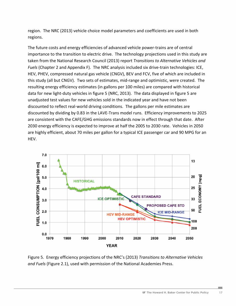
The future costs and energy efficiencies of advanced vehicle power-‐trains are of central importance to the transition to electric drive. The technology projections used in this study are taken from the National Research Council (2013) report Transitions to Alternative Vehicles and
Fuels (Chapter 2 and Appendix F). The NRC analysis included six drive-‐train technologies: ICE, HEV, PHEV, compressed natural gas vehicle (CNGV), BEV and FCV, five of which are included in this study (all but CNGV). Two sets of estimates, mid-‐range and optimistic, were created. The resulting energy efficiency estimates (in gallons per 100 miles) are compared with historical data for new light-‐duty vehicles in figure 5 (NRC, 2013). The data displayed in figure 5 are unadjusted test values for new vehicles sold in the indicated year and have not been discounted to reflect real-‐world driving conditions. The gallons per mile estimates are discounted by dividing by 0.83 in the LAVE-‐Trans model runs. Efficiency improvements to 2025 are consistent with the CAFE/GHG emissions standards now in effect through that date. After 2030 energy efficiency is expected to improve at half the 2005 to 2030 rate. Vehicles in 2050 are highly efficient, about 70 miles per gallon for a typical ICE passenger car and 90 MPG for an HEV.
Figure 5. Energy efficiency projections of the NRC’s (2013) Transitions to Alternative Vehicles and Fuels (Figure 2.1), used with permission of the National Academies Press.

The Howard H. Baker Center for Public Policy18
The NRC (2013) assessment is one of the few that projects technological progress to 2050 and appears to be the only one that incorporates major reductions in vehicle loads (mass, aerodynamic drag, rolling resistance and accessories) and their synergistic benefits for vehicle manufacturing costs (e.g., engine downsizing, reduced battery size and weight, etc.) as well as energy conversion efficiencies. For example, in the mid-‐range case the weight of a typical passenger car in 2030 is 20% less than a 2010 vehicle; by 2050 a typical passenger car weighs 30% less than a comparable 2010 vehicle. Weight reductions for light-‐trucks designed for towing and hauling are smaller: 15% by 2030 and 22% by 2050. Aerodynamic drag and tire rolling resistances are also greatly improved.
Driven by increasingly rigorous fuel economy and emissions standards, the fuel economy of ICEs and HEVs increases nearly fourfold over 2010 levels and that of BEVs and FCVs nearly doubles (figures 6a & 6b). PHEVs10 are assumed to get the same fuel economy as BEVs when operating in charge-‐depleting mode and the same as HEVs when operating in charge-‐sustaining mode.
6(a)
6(b)
10 PHEVs are assumed to be PHEV30s with a 25 mile all-‐electric real world range.
0
50
100
150
200
250
2010 2020 2030 2040 2050
EPA Test Combined MPG
New Light-‐duty Vehicle Fuel Economy: Mid-‐range
PC BEV
LT BEV
PC FC
LT FCV
PC HEV
PC ICE
LT HEV
LT ICE
0
50
100
150
200
250
2010 2020 2030 2040 2050
EPA Test Combined MPG
New Light-‐duty Vehicle Fuel Economy: Optimistic
PC BEV
LT BEV
PC FC
LT FCV
PC HEV
PC ICE
LT HEV
LT ICE
Figure 6a and 6b. EPA Test Combined Fuel Economies by Technology Type: Mid-‐Range and Optimistic Estimates (NRC, 2013)
The NRC’s longer time frame and focus on load reduction produced two novel conclusions. First, because the cost of battery-‐electric and fuel cell power-‐trains scale more directly with power than ICE power-‐trains, load reduction is of greater value to these technologies. Second, unlike previous assessments extending to 2035 (e.g., Bandivadekar et al., 2008), after 2040 BEVs and FCVs become less costly than comparable ICEs or HEVs. PHEVs, on the other hand, remain a few thousand dollars more expensive through 2050 (figures 7a & 7b) because they require a powerful electric motor, an internal combustion engine and a substantial battery pack. Other studies have projected the narrowing of cost differences over time (e.g., element energy, 2011; McKinsey, 2011; Kromer and Heywood, 2007) but the crossover predicted by the NRC study is a new development. These new projections increase the likelihood of accomplishing a self-‐sustaining transition to electric drive vehicles. The cost estimates shown in figures 7a and 7b assume fully-‐learned, high-‐volume production (at least 200,000 units per year). In the LAVE-‐Trans model, these costs must be achieved over time through cumulative production and the growth of market demand. Costs in the early years of a transition will be far higher.
7(a) $0
$5,000
$10,000
$15,000
$20,000
$25,000
$30,000
$35,000
$40,000
$45,000
$50,000
2010 2020 2030 2040 2050
2009 Dollars
Retail Price Equivalents: Passenger CarsHigh Volume, Fully Learned
BEV
PHEV
FCV
HEV
ICE
The NRC (2013) assessment is one of the few that projects technological progress to 2050 and appears to be the only one that incorporates major reductions in vehicle loads (mass, aerodynamic drag, rolling resistance and accessories) and their synergistic benefits for vehicle manufacturing costs (e.g., engine downsizing, reduced battery size and weight, etc.) as well as energy conversion efficiencies. For example, in the mid-range case the weight of a typical passenger car in 2030 is 20% less than a 2010 vehicle; by 2050 a typical passenger car weighs 30% less than a comparable 2010 vehicle. Weight reductions for light-trucks designed for towing and hauling are smaller: 15% by 2030 and 22% by 2050. Aerodynamic drag and tire rolling resistances are also greatly improved.
Driven by increasingly rigorous fuel economy and emissions standards, the fuel economy of ICEs and HEVs increases nearly fourfold over 2010 levels and that of BEVs and FCVs nearly doubles (figures 6a & 6b). PHEVs10 are assumed to get the same fuel economy as BEVs when operating in charge-depleting mode and the same as HEVs when operating in charge-sustaining mode.
6(a)
6(b)
10 PHEVs are assumed to be PHEV30s with a 25 mile all-electric real world range.
0
50
100
150
200
250
2010 2020 2030 2040 2050
EPA
Tes
t Com
bine
d M
PG
New Light-duty Vehicle Fuel Economy: Mid-range
PC BEV
LT BEV
PC FC
LT FCV
PC HEV
PC ICE
LT HEV
LT ICE
0
50
100
150
200
250
2010 2020 2030 2040 2050
EPA
Tes
t Com
bine
d M
PG
New Light-duty Vehicle Fuel Economy: Optimistic
PC BEV
LT BEV
PC FC
LT FCV
PC HEV
PC ICE
LT HEV
LT ICE

The Howard H. Baker Center for Public Policy The Howard H. Baker Center for Public Policy 19
Figure 6a and 6b. EPA Test Combined Fuel Economies by Technology Type: Mid-‐Range and Optimistic Estimates (NRC, 2013)
The NRC’s longer time frame and focus on load reduction produced two novel conclusions. First, because the cost of battery-‐electric and fuel cell power-‐trains scale more directly with power than ICE power-‐trains, load reduction is of greater value to these technologies. Second, unlike previous assessments extending to 2035 (e.g., Bandivadekar et al., 2008), after 2040 BEVs and FCVs become less costly than comparable ICEs or HEVs. PHEVs, on the other hand, remain a few thousand dollars more expensive through 2050 (figures 7a & 7b) because they require a powerful electric motor, an internal combustion engine and a substantial battery pack. Other studies have projected the narrowing of cost differences over time (e.g., element energy, 2011; McKinsey, 2011; Kromer and Heywood, 2007) but the crossover predicted by the NRC study is a new development. These new projections increase the likelihood of accomplishing a self-‐sustaining transition to electric drive vehicles. The cost estimates shown in figures 7a and 7b assume fully-‐learned, high-‐volume production (at least 200,000 units per year). In the LAVE-‐Trans model, these costs must be achieved over time through cumulative production and the growth of market demand. Costs in the early years of a transition will be far higher.
7(a) $0
$5,000
$10,000
$15,000
$20,000
$25,000
$30,000
$35,000
$40,000
$45,000
$50,000
2010 2020 2030 2040 2050
2009 Dollars
Retail Price Equivalents: Passenger CarsHigh Volume, Fully Learned
BEV
PHEV
FCV
HEV
ICE
Figure 6a and 6b. EPA Test Combined Fuel Economies by Technology Type: Mid-Range and Optimistic Estimates (NRC, 2013)
The NRC’s longer time frame and focus on load reduction produced two novel conclusions. First, because the cost of battery-electric and fuel cell power-trains scale more directly with power than ICE power-trains, load reduction is of greater value to these technologies. Second, unlike previous assessments extending to 2035 (e.g., Bandivadekar et al., 2008), after 2040 BEVs and FCVs become less costly than comparable ICEs or HEVs. PHEVs, on the other hand, remain a few thousand dollars more expensive through 2050 (figures 7a & 7b) because they require a powerful electric motor, an internal combustion engine and a substantial battery pack. Other studies have projected the narrowing of cost differences over time (e.g., element energy, 2011; McKinsey, 2011; Kromer and Heywood, 2007) but the crossover predicted by the NRC study is a new development. These new projections increase the likelihood of accomplishing a self-sustaining transition to electric drive vehicles. The cost estimates shown in figures 7a and 7b assume fully-learned, high-volume production (at least 200,000 units per year). In the LAVE-Trans model, these costs must be achieved over time through cumulative production and the growth of market demand. Costs in the early years of a transition will be far higher.
7(a)
$0
$5,000
$10,000
$15,000
$20,000
$25,000
$30,000
$35,000
$40,000
$45,000
$50,000
2010 2020 2030 2040 2050
2009
Dol
lars
Retail Price Equivalents: Passenger CarsHigh Volume, Fully Learned
BEV
PHEV
FCV
HEV
ICE
7(b)
Figures 7a and 7b. Retail Price Equivalents (Long-run Average Costs)11 of Advanced Technologies at High Volume and Fully Learned, Mid-Range and Optimistic Estimates: Passenger Cars (NRC, 2013).
Reference energy prices are based on the Energy Information Administration’s 2011 Annual Energy Outlook (EIA, 2011). Low carbon energy prices are from the NRC (2013) Transitions study. Prices of gasoline, electricity and hydrogen for highway use are shown in figures 8a-8c. Regional prices were calculated by weighted averaging of prices for relevant Census Regions, provided in the EIA projections. In all scenarios, low-carbon hydrogen and a low-carbon electricity grid were assumed, and an indexed highway user fee (IHUF) was added to the price of all fuels. The indexed highway user fee assigns the motor fuel tax to all forms of energy used by light-duty vehicles and indexes the fee to the average miles per gallon of gasoline equivalent energy of the entire on-road vehicle stock. This prevents Highway Trust Fund revenues from being eroded by fuel economy improvements and insures a constant average level of revenue per vehicle mile traveled (Greene, 2011b).
Assuming the AEO Reference Oil Price projection and including the IHUF, gasoline prices rise from $3/gallon in 2010 to over $5/gallon by 2050 (figure 8a). Approximately $1 of that increase is due to the IHUF. The AEO Low Oil Price projection foresees prices dropping quickly and remaining at least a dollar below the Reference prices until after 2040. Oil prices are exogenous to the LAVE-Trans model and do not change as oil use by U.S. light-duty vehicles decreases.
11 Retail price equivalents include mark-ups over manufacturing costs and normal returns on investment.
$0
$10,000
$20,000
$30,000
$40,000
$50,000
$60,000
$70,000
2010 2020 2030 2040 2050
2009
Dol
lars
Retail Price Equivalents: Light Trucks High Volume, Fully Learned
BEV
PHEV
FCV
HEV
ICE
Figures 7a and 7b. Retail Price Equivalents (Long- -run Average Costs)11 of Advanced Technologies at High Volume and Fully Learned, Mid- -Range and Optimistic Estimates: Passenger Cars (NRC, 2013).

The Howard H. Baker Center for Public Policy20
7(b)
Figures 7a and 7b. Retail Price Equivalents (Long-‐run Average Costs)11 of Advanced Technologies at High Volume and Fully Learned, Mid-‐Range and Optimistic Estimates: Passenger Cars (NRC, 2013).
Reference energy prices are based on the Energy Information Administration’s 2011 Annual Energy Outlook (EIA, 2011). Low carbon energy prices are from the NRC (2013) Transitions study. Prices of gasoline, electricity and hydrogen for highway use are shown in figures 8a-‐8c. Regional prices were calculated by weighted averaging of prices for relevant Census Regions, provided in the EIA projections. In all scenarios, low-‐carbon hydrogen and a low-‐carbon electricity grid were assumed, and an indexed highway user fee (IHUF) was added to the price of all fuels. The indexed highway user fee assigns the motor fuel tax to all forms of energy used by light-‐duty vehicles and indexes the fee to the average miles per gallon of gasoline equivalent energy of the entire on-‐road vehicle stock. This prevents Highway Trust Fund revenues from being eroded by fuel economy improvements and insures a constant average level of revenue per vehicle mile traveled (Greene, 2011b).
Assuming the AEO Reference Oil Price projection and including the IHUF, gasoline prices rise from $3/gallon in 2010 to over $5/gallon by 2050 (figure 8a). Approximately $1 of that increase is due to the IHUF. The AEO Low Oil Price projection foresees prices dropping quickly and remaining at least a dollar below the Reference prices until after 2040. Oil prices are exogenous to the LAVE-‐Trans model and do not change as oil use by U.S. light-‐duty vehicles decreases.
11 Retail price equivalents include mark-‐ups over manufacturing costs and normal returns on investment.
$0
$10,000
$20,000
$30,000
$40,000
$50,000
$60,000
$70,000
2010 2020 2030 2040 2050
2009 Dollars
Retail Price Equivalents: Light Trucks High Volume, Fully Learned
BEVPHEV
FCV
HEVICE

The Howard H. Baker Center for Public Policy The Howard H. Baker Center for Public Policy 21
8(a)
Imposing road user taxes on electricity initially adds about 1 cent per kWh to the average retail price. In the long run the IHUF grows to almost 4 cents per kWh (figure 8b). The cost of low carbon electricity increases gradually to about 5 cents per kWh in 2050. The costs are based on the NRC (2013) Transitions study which also starts with the AEO 2011 energy price projections.
8(b)
According to the assumptions of the NRC report, the retail price of hydrogen is initially above $10/kg due to the high cost of supplying hydrogen in small volumes and the high cost of operating refueling outlets below design capacity (Figure 8c). The initial, small volumes of hydrogen are produced by reforming of natural gas without carbon capture and storage. Lower GHG hydrogen, which becomes available after 2030, costs approximately $0.75/gge more than hydrogen produced from natural gas without carbon capture. Hydrogen prices are also taken from the NRC (2013) Transitions study.
$0.00
$1.00
$2.00
$3.00
$4.00
$5.00
$6.00
2010 2020 2030 2040 2050
2009 $/gallon
Retail Gasoline Price in California and Section 177 States
CA-‐ZEV Reference
CA-‐ZEV Ref no tax
CA-‐ZEV Low Oil Price
$0.00
$0.02
$0.04
$0.06
$0.08
$0.10
$0.12
$0.14
$0.16
$0.18
$0.20
2010 2020 2030 2040 2050
2009 $/kWh
Electricity Price in California and Section 177 States
CA-‐ZEV Low C
CA-‐ZEV Low C no tax
CA-‐ZEV Base no tax
8(a)
Imposing road user taxes on electricity initially adds about 1 cent per kWh to the average retail price. In the long run the IHUF grows to almost 4 cents per kWh (figure 8b). The cost of low carbon electricity increases gradually to about 5 cents per kWh in 2050. The costs are based on the NRC (2013) Transitions study which also starts with the AEO 2011 energy price projections.
8(b)
According to the assumptions of the NRC report, the retail price of hydrogen is initially above $10/kg due to the high cost of supplying hydrogen in small volumes and the high cost of operating refueling outlets below design capacity (Figure 8c). The initial, small volumes of hydrogen are produced by reforming of natural gas without carbon capture and storage. Lower GHG hydrogen, which becomes available after 2030, costs approximately $0.75/gge more than hydrogen produced from natural gas without carbon capture. Hydrogen prices are also taken from the NRC (2013) Transitions study.
$0.00
$1.00
$2.00
$3.00
$4.00
$5.00
$6.00
2010 2020 2030 2040 2050
2009
$/g
allo
nRetail Gasoline Price in California and Section 177 States
CA-ZEV Reference
CA-ZEV Ref no tax
CA-ZEV Low Oil Price
$0.00
$0.02
$0.04
$0.06
$0.08
$0.10
$0.12
$0.14
$0.16
$0.18
$0.20
2010 2020 2030 2040 2050
2009
$/k
Wh
Electricity Price in California and Section 177 States
CA-ZEV Low C
CA-ZEV Low C no tax
CA-ZEV Base no tax

The Howard H. Baker Center for Public Policy22
8(c)
Figures 8a, 8b and 8c. Energy Prices Used in the LAVE-‐Trans Model Runs.
All the scenarios considered in this report assume that the energy sources for advanced vehicles will be de-‐carbonized. The well-‐to-‐wheels greenhouse gas emission estimates and costs of de-‐carbonization are taken from the NRC (2013) report. Details can be found in chapter 3 and appendix G of that report. The fossil carbon content of gasoline is gradually reduced by the replacement of up to 38% of gasoline with synthetic gasoline derived from biomass via pyrolysis and refining. U.S. average emissions are shown in figure 9 for a particular scenario in which both fuel cell vehicles and battery electric vehicles are successful; emissions from electricity and other fuels in California will be lower due to the different primary energy sources used to generate electricity and the Low Carbon Fuels Standard. At low volumes, hydrogen is assumed to be produced from fossil fuels without carbon capture and storage. Once hydrogen use begins to increase rapidly, the additional hydrogen is assumed to be produced primarily from renewable energy or natural gas with carbon capture and sequestration. The transition seems very rapid but this is because new hydrogen production is assumed to be low-‐C and because production is increasing rapidly from a very low level. Although the carbon intensity of electricity is initially very high, the much greater energy efficiency of electric vehicles more than offsets the difference. In the long-‐run the carbon intensity of electricity is decreased to less than one-‐fourth of its 2010 level.
$0.00
$2.00
$4.00
$6.00
$8.00
$10.00
$12.00
2010 2020 2030 2040 20502009 $/Gallon of Gasoline Equivalent
Hydrogen Price in California and Section 177 States
CA-‐ZEV Low C
CA-‐ZEV High-‐C
8(c)
Figures 8a, 8b and 8c. Energy Prices Used in the LAVE-Trans Model Runs.
All the scenarios considered in this report assume that the energy sources for advanced vehicles will be de-carbonized. The well-to-wheels greenhouse gas emission estimates and costs of de-carbonization are taken from the NRC (2013) report. Details can be found in chapter 3 and appendix G of that report. The fossil carbon content of gasoline is gradually reduced by the replacement of up to 38% of gasoline with synthetic gasoline derived from biomass via pyrolysis and refining. U.S. average emissions are shown in figure 9 for a particular scenario in which both fuel cell vehicles and battery electric vehicles are successful; emissions from electricity and other fuels in California will be lower due to the different primary energy sources used to generate electricity and the Low Carbon Fuels Standard. At low volumes, hydrogen is assumed to be produced from fossil fuels without carbon capture and storage. Once hydrogen use begins to increase rapidly, the additional hydrogen is assumed to be produced primarily from renewable energy or natural gas with carbon capture and sequestration. The transition seems very rapid but this is because new hydrogen production is assumed to be low-C and because production is increasing rapidly from a very low level. Although the carbon intensity of electricity is initially very high, the much greater energy efficiency of electric vehicles more than offsets the difference. In the long-run the carbon intensity of electricity is decreased to less than one-fourth of its 2010 level.
$0.00
$2.00
$4.00
$6.00
$8.00
$10.00
$12.00
2010 2020 2030 2040 2050
2009
$/G
allo
n of
Gas
olin
e Eq
uiva
lent
Hydrogen Price in California and Section 177 States
CA-ZEV Low C
CA-ZEV High-C

The Howard H. Baker Center for Public Policy The Howard H. Baker Center for Public Policy 23
Figure 9. Well-‐to-‐Wheel Greenhouse Gas Emissions from Vehicle Fuels, U.S. Averages.
Transitioning to electric drive vehicles is a complex process that requires policy initiatives of many types, from adjusting codes and standards to mandates or subsidies for vehicles and fuels (e.g., Gallagher et al., 2012). In the scenario analyses that follow we focus on just two: 1) early provision of refueling and recharging infrastructure through mandates and/or subsidies and, 2) incentivizing early vehicle sales through subsidies and/or mandates. This is done to simplify the modeling and is not a policy recommendation. In fact, who pays the additional costs of the early infrastructure and electric drive vehicle sales is not specified. Current policies are continued until they expire. In the future, governments may elect to subsidize all or part of the additional transition costs or may transfer the burden to vehicle manufacturers, energy suppliers and consumers by means of regulatory requirements.
Two key policies are assumed to remain in effect and be strengthened over time: 1) fuel economy and emissions standards and 2) renewable and low carbon fuels standards. The effect of fuel economy standards was described in the previous section. Consistent with the assumptions of the NRC’s Transitions to Alternative Vehicles and Fuels report, ethanol continues to be blended with gasoline up to 10 billion gallons per year gasoline equivalent. Additionally, “drop-‐in” biofuel, chemically equivalent to gasoline is produced from cellulosic biomass via pyrolysis and refining. It is expected to cost $3 to $4 per gallon, before tax. Production grows to 13.5 billion gallons in 2030 and remains at that level through 2050 (NRC, 2013, p. 92).
The California Zero Emission Vehicle regulation is the key policy promoting the early marketing of electric drive vehicles in California and the Section 177 states. The regulation is a technology-‐neutral performance requirement that mandates that a portion of each major
0
5
10
15
20
25
2010 2020 2030 2040 2050
kg CO2/GGE
Well-‐to-‐Wheel GHG Emissions of Vehicle Fuels
Electricity
Gasoline
Hydrogen
Figure 9. Well-to-Wheel Greenhouse Gas Emissions from Vehicle Fuels, U.S. Averages.
Transitioning to electric drive vehicles is a complex process that requires policy initiatives of many types, from adjusting codes and standards to mandates or subsidies for vehicles and fuels (e.g., Gallagher et al., 2012). In the scenario analyses that follow we focus on just two: 1) early provision of refueling and recharging infrastructure through mandates and/or subsidies and, 2) incentivizing early vehicle sales through subsidies and/or mandates. This is done to simplify the modeling and is not a policy recommendation. In fact, who pays the additional costs of the early infrastructure and electric drive vehicle sales is not specified. Current policies are continued until they expire. In the future, governments may elect to subsidize all or part of the additional transition costs or may transfer the burden to vehicle manufacturers, energy suppliers and consumers by means of regulatory requirements.
Two key policies are assumed to remain in effect and be strengthened over time: 1) fuel economy and emissions standards and 2) renewable and low carbon fuels standards. The effect of fuel economy standards was described in the previous section. Consistent with the assumptions of the NRC’s Transitions to Alternative Vehicles and Fuels report, ethanol continues to be blended with gasoline up to 10 billion gallons per year gasoline equivalent. Additionally, “drop-in” biofuel, chemically equivalent to gasoline is produced from cellulosic biomass via pyrolysis and refining. It is expected to cost $3 to $4 per gallon, before tax. Production grows to 13.5 billion gallons in 2030 and remains at that level through 2050 (NRC, 2013, p. 92).
The California Zero Emission Vehicle regulation is the key policy promoting the early marketing of electric drive vehicles in California and the Section 177 states. The regulation is a technology-neutral performance requirement that mandates that a portion of each major
0
5
10
15
20
25
2010 2020 2030 2040 2050
kg C
O2/
GG
EWell-to-Wheel GHG Emissions of Vehicle Fuels
Electricity
Gasoline
Hydrogen

The Howard H. Baker Center for Public Policy24
manufacturer’s sales must have zero tailpipe emissions (Shulock et al., 2011). The scenarios presented below are based on California Air Resources Board staff estimates and suggest that in the initial phase in years 2015-‐2017, manufacturers are likely to sell 6,500 to 7,000 hydrogen fuel cell vehicles (FCVs), approximately 20,000 battery electric vehicles (BEVs) and 80,000 transitional zero emission vehicles (most likely plug-‐in hybrid electric vehicle: PHEVs) in California and Section 177 states12. Through 2025, the ARB estimates sales of nearly 1 million TZEVs13, about 385,000 BEVs and approximately 170,000 FCVs. The heavy weighting in favor of plug-‐in vehicles partly reflects the “travel” provision of the ZEV mandate, which allows fuel cell vehicles sold in California to count in the other Section 177 states. The provision reflects the earlier presence of plug-‐in vehicles in the market, as well as the initial challenge of establishing a hydrogen refueling infrastructure. Detailed assumptions about vehicle sales under the ZEV scenarios can be found in appendix table A.1.
California’s plan for deploying hydrogen refueling stations begins with the strategic placement of 68 stations in five linked clusters (CAFCP, 2012) during a pre-‐commercial period from 2012 to 2014 (Table 2). Clustering the stations allows a density of hydrogen stations equivalent to about 5-‐7% of the gasoline stations in the local areas where they will be clustered. This will be far less than 5-‐7% of the gasoline stations in California; more like 0.5-‐0.7%. Once these stations are in place, the plan is to increase the number of stations as vehicle sales grow. The California Fuel Cell Partnership’s (CAFCP) 68 station deployment plan is the basis for our assumptions about early hydrogen station availability. When the rest of the U.S. adopts similar transition policies, 324 mandated or subsidized stations are assumed to be deployed before 2020. Once the early infrastructure has been deployed, the number of stations is assumed to increase with hydrogen demand.
Success of the ZEV program in California and the Section 177 states would likely induce other states and the federal government to join in the effort. In the standard policy scenario used in this report (Scenario 2 of the first report: Greene et al., 2013a) the rest of the U.S. adopts similar transition policies to California with a five year lag. U.S. transition policies include both early infrastructure deployment and mandates or subsidies for ZEVs. However, the per-‐vehicle subsidies in the rest of the U.S. are lower than required to meet ZEV requirements in California and the Section 177 states because of the external benefits created by the ZEV mandate. By 2050, 75% of new vehicle sales are FCVs, PHEVs or BEVs and most of the remainder are HEVs (figure 10). Sixty percent of the light-‐duty vehicles on the road are estimated to be electric drive by 2050 and another 15% are hybrids.
12For details, see Appendix table A.1. 13 Transitional Zero Emission Vehicles (TZEV) were formerly referred to as “Enhanced Advanced Technology Partial Zero Emission Vehicles (Enhanced AT-‐PZEV). This category includes plug-‐in hybrids and hydrogen internal combustion engine vehicles.

The Howard H. Baker Center for Public Policy The Howard H. Baker Center for Public Policy 25
Figure 10. Estimated Sales by Technology in California and the Section 177 States: Scenario 2.
The transition to electric drive vehicles, combined with low-‐carbon electricity, hydrogen and gasoline (4.6 billion gallons or 35% of which is produced thermo-‐chemically from biomass), achieves a 79% reduction in GHG emissions and virtually eliminates petroleum use by light-‐duty vehicles by 2050 (figure 11).
Figure 11. Changes in Petroleum Use and GHG Emissions vs. 2005 in California and the Section 177 States: Scenario 2
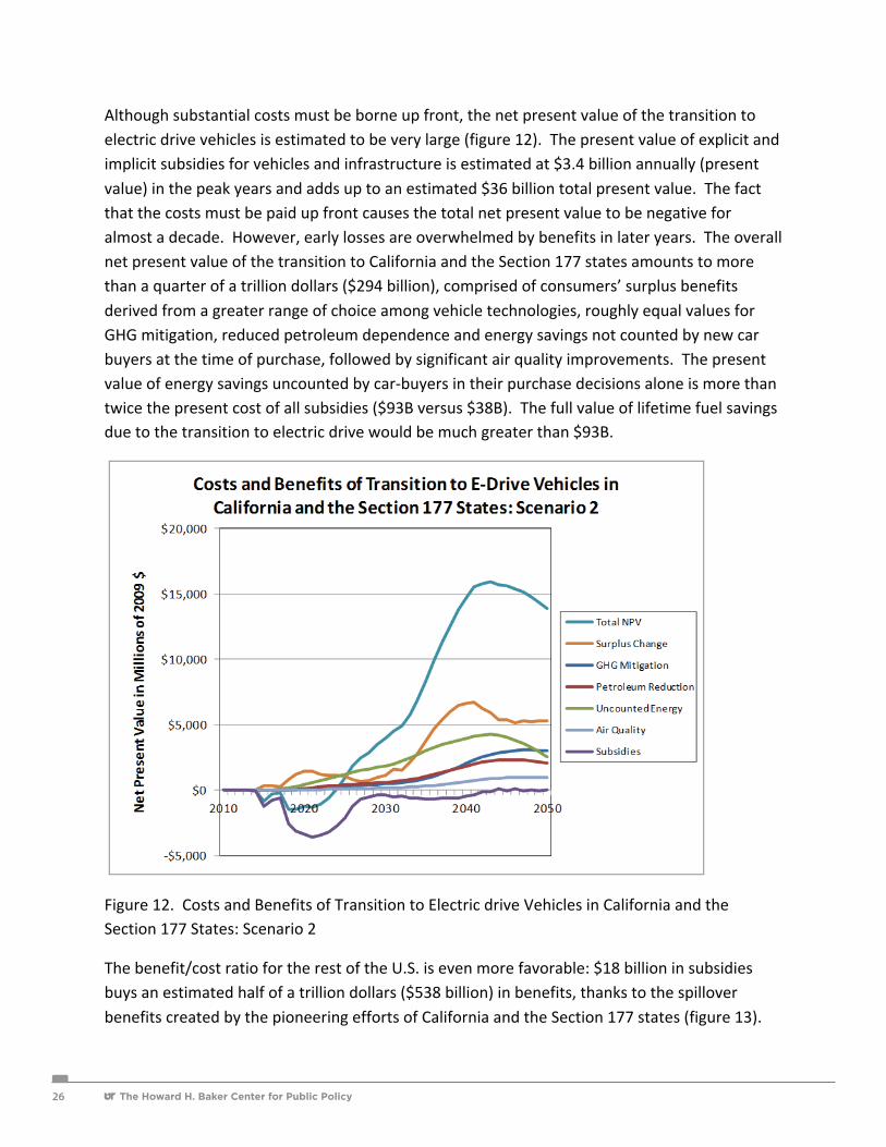
The Howard H. Baker Center for Public Policy26
Although substantial costs must be borne up front, the net present value of the transition to electric drive vehicles is estimated to be very large (figure 12). The present value of explicit and implicit subsidies for vehicles and infrastructure is estimated at $3.4 billion annually (present value) in the peak years and adds up to an estimated $36 billion total present value. The fact that the costs must be paid up front causes the total net present value to be negative for almost a decade. However, early losses are overwhelmed by benefits in later years. The overall net present value of the transition to California and the Section 177 states amounts to more than a quarter of a trillion dollars ($294 billion), comprised of consumers’ surplus benefits derived from a greater range of choice among vehicle technologies, roughly equal values for GHG mitigation, reduced petroleum dependence and energy savings not counted by new car buyers at the time of purchase, followed by significant air quality improvements. The present value of energy savings uncounted by car-‐buyers in their purchase decisions alone is more than twice the present cost of all subsidies ($93B versus $38B). The full value of lifetime fuel savings due to the transition to electric drive would be much greater than $93B.
Figure 12. Costs and Benefits of Transition to Electric drive Vehicles in California and the Section 177 States: Scenario 2
The benefit/cost ratio for the rest of the U.S. is even more favorable: $18 billion in subsidies buys an estimated half of a trillion dollars ($538 billion) in benefits, thanks to the spillover benefits created by the pioneering efforts of California and the Section 177 states (figure 13).
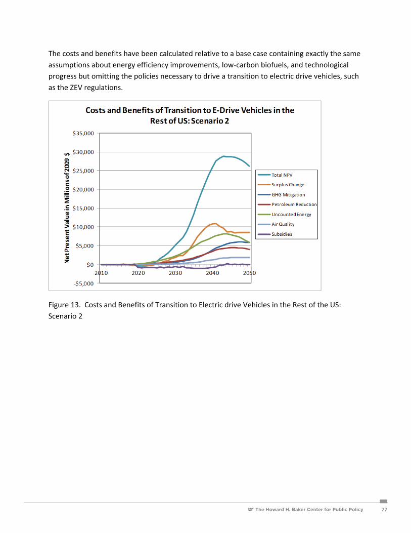
The Howard H. Baker Center for Public Policy The Howard H. Baker Center for Public Policy 27
The costs and benefits have been calculated relative to a base case containing exactly the same assumptions about energy efficiency improvements, low-‐carbon biofuels, and technological progress but omitting the policies necessary to drive a transition to electric drive vehicles, such as the ZEV regulations.
Figure 13. Costs and Benefits of Transition to Electric drive Vehicles in the Rest of the US: Scenario 2

The Howard H. Baker Center for Public Policy28
IV. Network External Benefits and Policy Feedback Effects
The effects of public policies like the ZEV requirements on the transition to electric drive vehicles will be complex and characterized by multiple feedback mechanisms. In this section the mathematics of only one such mechanism as it is represented in the LAVE-‐Trans model are spelled out. Following that, the impacts of increasing net subsidies, first for BEVs and then FCVs, are analyzed using the LAVE-‐Trans model to illustrate the potential magnitude of feedback effects. The examples also illustrate the importance of the timing and context of policies to encourage alternative energy vehicles. The analysis can only reflect the relationships and assumptions embodied in the LAVE-‐Trans model and so should be interpreted with caution. Nonetheless, the feedback effects illustrated exist and there appear to be some useful generalizations for public policy making.
A change in the subsidy of an electric drive vehicle may be a payment by government to a consumer, or manufacturers may be induced to subsidize electric drive vehicles by a regulatory requirement, such as the ZEV mandate. Starting with the Net Present Value (NPV) of the transition we analyze the effect of a change in the subsidy to one type of electric drive vehicle on just one component of the utility index: the risk aversion of majority consumers. Having illustrated mathematically one pathway by which policy can induce a positive feedback effect, we then use the LAVE-‐Trans model to quantify the full range of feedback effects included in the model.
The Net Present Value of a transition is defined as the sum over the relevant time intervals of changes in six components (equation 7), comparing the electric drive transition (designated by the subscript E) relative to the Base Case (subscripted B):
1. The consumers’ surplus of new vehicle buyers, CS, 2. Subsidies to vehicles, fuels and infrastructure, S, 3. The change in energy costs not considered by purchasers of vehicles at the time of
purchase, CE, 4. The change in GHG emission damages, GHG, 5. The change in local air pollution damages, AQ, 6. The change in energy security costs, ES.
Equation 7
!"# =1
(1+ !)! !"!" − !"!" + !!" − !!" + !"!" − !"!" + !"!!" − !"!!"!
!!!+ !"!" − !"!" + !"!" − !"!"

The Howard H. Baker Center for Public Policy The Howard H. Baker Center for Public Policy 29
The change in net present value is a partial equilibrium result in that the economy-‐wide effects of the measured costs and benefits are not considered. Changing a subsidy for vehicle technology i in year s < T will affect all six components. Most obviously it will increase the cost of subsidies, SEs, by an amount equal to the number of vehicles sold multiplied by the change in subsidy. But it will also increase subsidies in subsequent years. Consider the effect on only the consumers’ surplus component in year t of the energy transition, ΔCSEt., of a change in the subsidy offered to buyers of fuel cell vehicles.
Equation 8
∆!"!" = −1! !" !!!"
!"#+ !!!"
!"!!" + !" !!!"
!"#+ !!!"
!"!!" − !"!"
The term UBuy indicates the utility of the decision to purchase a new vehicle while UNo represents the utility of the decision to buy other things instead. The subscripts indicate market classes: M for majority consumers and I for innovators/early adopters, in year t. The number of majority consumer households is NMt, and the number of innovator/early-‐adopter households is NIt. The parameter β is the marginal utility of income, assumed for simplicity to be constant. If anything, using a constant β should make it more difficult for initially more expensive, advanced technology vehicles to begin to penetrate the market. A less price-‐sensitive market segment would be more likely to purchase the first few, more expensive, advanced technology vehicles. If incomes generally increased and price sensitivity decreased over time, initial sales of alternative technology vehicles might be more easily accomplished in the future. Such refinements are left for future model development.
The utility of the decision to buy a vehicle in the energy transition case is comprised of layers of nested utilities in the NMNL model. The utility of the Buy/No-‐Buy decision is affected by the utilities of cars and light trucks:
Equation 9
!!"!"# = !!
1!!!" !!!"
!"#+ !!!"
!"#$
And their utilities are affected by those of the ICE, BEV and FCV options:

The Howard H. Baker Center for Public Policy30
Equation 10
!!"!"# = !!1!!!" !!!"
!"#+ !!!"
!"#+ !!!"
!"#
And finally the utility of the FCV choice is affected by the change in subsidy via the price paid for the FCV, PFCV:
Equation 11
!!"!"# = !!1!!
!! !!"#$ − 100 + !!!"!"#$ + !!!!"#$ + !!!!"# !! − 1 + !!!"!"#
+ !!!"!!"#$!!
Four of the six arguments in the fuel cell vehicle utility equation are a function of previous sales of fuel cell vehicles. Cumulative sales drive down vehicle prices via learning by doing and they diminish the risk aversion (RA) of majority consumers, as well. The size of the stock of vehicles also affects refueling availability, f, by increasing the size of the market for hydrogen fuel. Increased sales reduce vehicle prices via scale economies, and increase the diversity of choice by increasing the number of makes and models to choose from. Increased sales may also increase fuel availability, f, by increasing demand for hydrogen fuel.
The complexity of feedback effects can be illustrated by looking at just one component of the utility function: the majority’s risk aversion. Consider the effect (derivative) of a change in the subsidy to fuel cell vehicles in year s on the majority’s risk aversion in year T.
Equation 12
!!"!"#!!!"#$
=!
!!!"#$!!! !!!
!!! = !"!! !!!!!!
!!!!!!
!!!!!!
!
!!!
At the far right of the equation, changing the subsidy for FCVs will increase sales of FCVs in year s. The second term, ∂Nt/∂Ns, is itself complex because a change in Ns affects Ns+1 which, in turn affects Ns+2 and so on up to NT-‐1, and all affect NT. The effect of an increase in the subsidies to fuel cell vehicles in year s will tend to grow due to the effect of cumulative vehicle sales but will also decrease as the marginal impact of cumulative sales decreases (ρ < 0). The effect is far more complex than shown here since increased sales will also induce positive feedbacks via scale economies, learning by doing, and diversity of make and model choice.

The Howard H. Baker Center for Public Policy The Howard H. Baker Center for Public Policy 31
These effects can be illustrated by the LAVE-‐Trans model. All of the examples are based on Scenario 2 in which the ZEV mandates, followed by similar US policies, successfully induce a transition to electric drive vehicles. A one-‐time, $100 net increase in the subsidy for BEVs in the year 2020 is considered first. 14 The impact of the subsidy on retail price equivalent, the willingness to pay of innovators and early adopters, and the perceived costs of majority risk aversion, fuel availability and diversity of make and model choices is shown in Figure 14a. All the values shown are changes from those of Scenario 2. The impact on price is immediate but, by assumption, lasts only one year as shown by the black line.15 The price change induces a small increase in sales of 2,000 BEVs in 2020 (figure 14b). The very small decrease in sales in 2021 is an artifact of the way the LAVE-‐Trans model calculates manufacturer subsidies and rebates induced by fuel economy standards. Feebates for the current year are based on the previous year’s sales distribution, which can induce oscillations in response to a price change.
Figure 14a. Impacts of a $100 Increase in the Net Subsidy per BEV in 2020 on Perceived Vehicle Utility.
14 If the ZEV requirements are causing manufacturers to sell more electric drive vehicles than they would have sold in the absence of the standards, the vehicles’ prices will have to be reduced by some combination of manufacturer and government subsidies. The analysis assumes a $100 increase in the total subsidy from all sources. If government subsidies were increased without a corresponding increase in ZEV requirements, manufacturers would likely decrease the subsidies they were providing. That is not the situation being analyzed here. Here a net increase of $100 in the combined subsidy makes the vehicles $100 cheaper to the customer. 15 In real-‐world markets, a $100 increase in subsidy would generally reduce market price by less than $100 unless vehicle supply were perfectly elastic. The example is intended solely to trace the effects of a change in net vehicle price and so such effects are not considered.
-‐$120
-‐$100
-‐$80
-‐$60
-‐$40
-‐$20
$0
$20
2010 2020 2030 2040 2050
Chan
ge in
Perceived
Cost p
er Car
Impacts of a $100 Increase in Net Subsidy per BEV in 2020
Innovator WTP
Public Recharge Avail.
Choice Diversity
Majority Risk
Price

The Howard H. Baker Center for Public Policy32
Figure 14b. Impacts of a $100 Increase in Net Subsidy per BEV in 2020 on BEV Sales.
The increased sales cause reductions in the risk aversion of majority consumers, an increase in make and model availability and an almost imperceptible benefit due to increased availability of public recharging infrastructure. There is also a cost, in the form of reduced willingness to pay by innovators and early adopters. Finally, there is a very small cost reduction due to learning by doing (figure 14c). The learning variable approaches 1 asymptotically as cumulative production increases. The scale economy parameter also approaches 1 from above as annual production volume increases.16 Thus, negative changes in comparison to Scenario 2 indicate cost reductions. Because the ZEV mandates have already brought total US sales of BEVs to just over 200,000 units per year in 2020, there is no benefit from increased scale economies. This is an artifact of the model, since in the real world increased sales would almost certainly continue to reduce costs. In the LAVE-‐Trans model full scale economies are reached at 200,000 units per year. In the real world, not only are there likely to be benefits to scale beyond 200,000 units per year but greater competition in supply chains at higher sales volumes would also likely yield additional cost reductions.
16 In the LAVE-‐Trans model, scale economies in year t are determined by the sales volume in year t-‐1. This is chiefly done for programming convenience to avoid simultaneity of prices and sales which would otherwise cause a circular reference in the LAVE-‐Trans spreadsheet model, requiring iterative solution in each year.
-‐1.0
0.0
1.0
2.0
3.0
4.0
5.0
6.0
2010 2020 2030 2040 2050
Chan
ge in
Sales (0
00)
Impacts of a $100 Increase in Net Subsidy per BEV in 2020

The Howard H. Baker Center for Public Policy The Howard H. Baker Center for Public Policy 33
Figure 14c. Impacts of a $100 Increase in Net Subsidy per BEV in 2020 on Scale Economies and Learning by Doing.
If the $100 net subsidy increase occurs earlier in 2015, the feedback effects are considerably smaller. There is the same one-‐time reduction in retail price but the induced effects on majority risk aversion, diversity of choice and innovator willingness to pay are much smaller (figure 15a). The smaller feedback effects are due to a much smaller increase in sales. In 2015, BEVs are substantially more expensive than in 2020 and, as a result, the increase in sales in 2015 is an order of magnitude smaller than the 2020 increase (figure 15b).
-‐0.00030
-‐0.00025
-‐0.00020
-‐0.00015
-‐0.00010
-‐0.00005
0.000002010 2020 2030 2040 2050
Chan
ge in
Param
eter Value
Impacts of a $100 Increase in Net Subsidy per BEV in 2020
Scale Effect
Learning Effect

The Howard H. Baker Center for Public Policy34
Figure 15a. Impacts of a $100 Increase in Net Subsidy per BEV in 2015 on Perceived Vehicle Utility.
Figure 15b. Impacts of a $100 Increase in Net Subsidy per BEV in 2015 on Vehicle Sales.
-‐$120
-‐$100
-‐$80
-‐$60
-‐$40
-‐$20
$0
$20
2010 2020 2030 2040 2050
Chan
ge in
Perceived
Cost p
er Car
Impacts of a $100 Increase in Net Subsidy per BEV in 2015
Innovator WTP
Public Recharge Avail.
Choice Diversity
Majority Risk
Price
-‐0.2
0.0
0.2
0.4
0.6
0.8
1.0
2010 2020 2030 2040 2050
Chan
ge in
Sales (0
00)
Impacts of a $100 Increase in Net Subsidy per BEV in 2015

The Howard H. Baker Center for Public Policy The Howard H. Baker Center for Public Policy 35
Again, starting with Scenario 2, the subsidy to fuel cell vehicles (cars and light trucks) is increased by $100 in California and the Section 177 states, but only in year 2020. The effects over time on the utility of a fuel cell passenger car in those states (differences from Scenario 2) are illustrated in figure 16a. In 2020, there is an immediate reduction in price of $100, as would be expected (black line). The effect increases somewhat in 2021 due to scale economies and learning. Sales in California have a spillover effect on sales in the rest of the U.S. one year later, due to the 1-‐year lagged connection between the two markets. Driven by positive feedback effects in both markets, FCV prices drop rapidly to almost $1,000 below the Reference Scenario 2 level in 2026. Beyond 2025 prices are the same in both scenarios because total U.S. sales reach 200,000 units annually and opportunities for learning in the manufacture of the new technology are nearly exhausted. Other feedbacks continue, however. The greater number of FCVs sold reduces the majority’s aversion to risk by almost $600 by 2027 (green line) and reduces the cost of fuel availability by about $100 (blue line) in comparison to the same scenario without the increased subsidy in 2020. Diversity of choice is also improved (red line), although the perceived cost oscillates due to the LAVE-‐Trans feebate algorithm, as described above. There is a loss of novelty value to innovators of about $200 (purple line). All the effects wear off by 2050 as market demand reaches an unsubsidized sustainable level.
Figure 16a. Impacts of a $100 Increase in Net Subsidy per FCV in 2020 on Perceived Vehicle Utility.
-‐$1,000
-‐$800
-‐$600
-‐$400
-‐$200
$0
$200
$400
2010 2020 2030 2040 2050
Chan
ge in
Perceived
Cost p
er Car
Impacts of a $100 Increase in Net Subsidy per FCV in 2020
Innovator WTP Fuel Availability Choice Diversity Majority Risk Price

The Howard H. Baker Center for Public Policy36
Figure 16b. Impacts of a $100 Increase in Net Subsidy per FCV in 2020 on Vehicle Sales.
The increased subsidy in 2020 immediately increases sales in comparison to the Scenario 2 reference case but only by a small amount, as the market for fuel cell vehicles is still very small (figure 16b). The benefit shrinks dramatically in 2026 when the FCV price difference falls to zero. However, as figure 16a illustrates, fuel availability and majority risk reduction benefits persist. In 2025, sales of FCVs are 67 thousand in the reference Scenario 2 case, 90 thousand in the increased subsidy case. In 2026, however, sales are 90 thousand in the reference Scenario 2 case, but only 93 thousand in the increased subsidy case. Yet because of the persistent effects of greater diversity of choice, lower majority risk aversion, and greater fuel availability in the increased subsidy case, sales grow more rapidly after 2030 than in the reference case. Positive feedbacks between the ZEV states and the rest of the U.S. amplify the effects. The advantage of the increased subsidy case expands until 2035. Although new FCV sales are identical in both cases by 2050, the NPV advantage persists due to the greater numbers of FCVs on the road in the increased subsidy case.
The price effect shown in figure 16a is mirrored in the reduction in the scale economy multiplier shown in figure 16c. The benefits of increased scale dissipate quickly because a production volume of almost 200,000 is reached in Scenario 2 by 2025. By 2027, both scenarios have exhausted the available scale economies. A very small learning by doing benefit persists, however.
0
50
100
150
200
250
2010 2020 2030 2040 2050
Chan
ge in
Sales (0
00)
Impacts of a $100 Increase in Net Subsidy per FCV in 2020

The Howard H. Baker Center for Public Policy The Howard H. Baker Center for Public Policy 37
Figure 16c. Impacts of a $100 Increase in Net Subsidy per FCV in 2020 on Scale Economies and Learning by Doing.
If the $100 increase in net subsidy to FCVs is made in 2015, the effect is very different (figure 17a). Not only is the retail price equivalent of an FCV in 2015 greater than $50,000 but FCVs also suffer from lack of fuel availability, majority risk aversion and lack of diversity of choice. Sales in California and ZEV states (where all U.S. sales are in 2015) are just 3,000 units. A $100 additional subsidy has very little impact on sales in 2015 (figure 17b). Just 60 more FCVs are sold. The price impact in 2015 is $100 and falls back to almost $0 the following year. The benefit of such a small increase in sales is barely noticeable for either scale economies or learning by doing (figure 17b). Benefits in fuel availability and majority risk aversion are also small. Sales increase relative to Scenario 2, but the increase is an order of magnitude smaller than that achieved by the same subsidy in 2020 (figures 16b and 17b). Surprisingly, the benefits of these small increments produce a second price benefit starting in 2020 when the rest of the U.S. implements policies promoting FCVs. The price “echo” is approximately the same size as the initial price subsidy but applies to a greater number of cars and requires no additional subsidy. Again, the price benefit drops to near zero in 2026, the year in which full scale economies are achieved in Scenario 2 (figure 17c).
-‐0.045
-‐0.040
-‐0.035
-‐0.030
-‐0.025
-‐0.020
-‐0.015
-‐0.010
-‐0.005
0.0002010 2020 2030 2040 2050
Chan
ge in
Param
eter Value
Impacts of a $100 Increase in Net Subsidy per FCV in 2020
Scale Effect
Learning Effect

The Howard H. Baker Center for Public Policy38
Figure 17a. Impacts of a $100 Increase in Net Subsidy per FCV in 2015 on Perceived Vehicle Utility.
Figure 17b. Impacts of a $100 Increase in Net Subsidy per FCV in 2015 on Vehicle Sales.
-‐$160
-‐$140
-‐$120
-‐$100
-‐$80
-‐$60
-‐$40
-‐$20
$0
$20
$40
2010 2020 2030 2040 2050
Chan
ge in
Perceived
Cost p
er Car
Impacts of a $100 Increase in Net Subsidy per FCV in 2015
Innovator WTP Fuel Availability Choice Diversity Majority Risk Price
0
5
10
15
20
25
30
2010 2020 2030 2040 2050
Chan
ge in
Sales (0
00)
Impacts of a $100 Increase in Net Subsidy per FCV in 2015

The Howard H. Baker Center for Public Policy The Howard H. Baker Center for Public Policy 39
Figure 17c. Impacts of a $100 Increase in Net Subsidy per FCV in 2015 on Scale Economies and Learning by Doing.
Delaying the $100 net subsidy increase to 2026, after full scale production has been reached results in an even smaller impact. The price impact is limited to 2026, although risk, diversity and fuel availability benefits persist at modest levels afterwards (figure 18a). Sales impacts begin at 1,500 vehicles in 2026 and eventually increase to 8,000 units per year before dissipating by 2050 (figure 18b). The total increase in FCV sales by 2050 is less than 70,000 units, compared with 200,000 units when the subsidy increase takes place in 2015, and just under 2 million when 2020 is the chosen year.
-‐0.006
-‐0.005
-‐0.004
-‐0.003
-‐0.002
-‐0.001
0.0002010 2020 2030 2040 2050
Chan
ge in
Param
eter Value
Impacts of a $100 Increase in Net Subsidy per FCV in 2015
Scale Effect
Learning Effect

The Howard H. Baker Center for Public Policy40
Figure 18a. Impacts of a $100 Increase in Net Subsidy per FCV in 2026 on Perceived Vehicle Utility.
Figure 18b. Impacts of a $100 Increase in Net Subsidy per FCV in 2026 on Vehicle Sales.
-‐$120
-‐$100
-‐$80
-‐$60
-‐$40
-‐$20
$0
$20
2010 2020 2030 2040 2050
Chan
ge in
Perceived
Cost p
er Car
Impacts of a $100 Increase in Net Subsidy per FCV in 2026
Innovator WTP Fuel Availability Choice Diversity Majority Risk Price
0.0
1.0
2.0
3.0
4.0
5.0
6.0
7.0
8.0
9.0
2010 2020 2030 2040 2050
Chan
ge in
Sales (0
00)
Impacts of a $100 Increase in Net Subsidy per FCV in 2026

The Howard H. Baker Center for Public Policy The Howard H. Baker Center for Public Policy 41
These results illustrating the self-‐reinforcing effects of positive feedbacks in the transition process indicate that the effects can be very strong. The powerful interactions between California and the Section 177 states and the rest of the U.S. not only underline the importance of the rest of the U.S. to the State of California but suggest that interactions between the U.S. and the rest of the world will also matter a great deal. This result echoes the results of Scenario X in the phase I report, which indicated that international effort to promote electric drive vehicles could be almost as important to the success of electric drive vehicles in California as federal policies.
Policies that appear to be having minor impacts early in the transition process appear to be able to produce much greater benefits later in the market transition. However, the examples presented above should not be interpreted to imply that it is always better to increase subsidies. The benefits of increased subsidies are conditional on the technological progress of the mid-‐range scenario and such technological progress, though likely, is not guaranteed. In addition, timing matters a great deal, as does the stage of market development. When the market has become relatively mature and further cost reductions through scale economies and learning by doing are likely to be small the leverage of subsidies is greatly diminished.

The Howard H. Baker Center for Public Policy42
V. Timing and Intensity of Policies
Beginning the transition to electric drive vehicles sooner allows more time to build up the stock of grid connected and hydrogen fuel cell vehicles. This allows greater substitution of alternative energy sources for petroleum and greater reduction in total GHG emissions. On the other hand, since technological progress reduces the high-‐volume manufacturing costs of electric drive vehicles, delaying the transition reduces the need for vehicle subsidies under the assumptions of Scenario 2. Delaying also allows more time for de-‐carbonization of electricity production. Several researchers have pointed out that today the GHG mitigation potential of grid connected vehicles is limited by the carbon intensity of electricity generation (Michalek et al., 2011; Ji et al., 2013). An additional, important consideration not addressed here is the potential to reduce the risk of failure by delaying the start of the transition until there is greater certainty of success. As will be shown in section VI, the risk of failure appears to be small, even allowing for substantial uncertainty with respect to the NRC’s (2013) technology projections.17 In this section, the question of timing is explored under the assumption that the future progress of technology is certain. All of the figures in this section illustrating cost and benefit impacts pertain to California and the Section 177 states only (not to the rest of the U.S.).
Four scenarios were run in which the ZEV requirements were assumed to begin earlier in 2011, as currently planned in 2015, and later in 2020 or 2025. In all cases 68 hydrogen stations are assumed to be in place the year before the ZEV requirements take effect. All other assumptions are the same as reference Scenario 2, including U.S. transition policies following five years behind the ZEV mandates. The estimated net present values are shown in figure 19.
17 A rigorous assessment of the risk of initiating a transition too soon would require an ability to adapt policies in the course of a model run depending on decision rules for accelerating, deceleration or terminating the transition. At present the LAVE-‐Trans model does not have such a capability and so the topic is left for future research.

The Howard H. Baker Center for Public Policy The Howard H. Baker Center for Public Policy 43
Figure 19. Impact of Delaying on the Net Present Value of the Transition to Electric Drive Vehicles in California and the Section 177 States.
Subsidies (shown in red) are smaller the longer the transition is delayed, reflecting the decreasing long-‐run, high-‐volume costs of electric drive vehicles over time. However, the savings in reduced subsidies are far outweighed by the losses of benefits. Delaying the ZEV requirements from 2015 to 2025 saves an estimated $23 billion in subsidies but at the expense of over $200 billion in foregone benefits within the ZEV states.18 The foregone additional energy savings alone ($55 billion) are more than twice the reduction in vehicle and infrastructure subsidies. The incremental cost (in lost benefits) of delaying from 2015 to 2020 is almost $80 billion while the incremental benefit (in reduced subsidy costs) is about $15 billion. In all cases, the costs and benefits of only those vehicles sold through 2050 are considered in the calculations. The costs and benefits of those vehicles are accounted for until 2075, by which time nearly all of them will have been retired.
The benefit/cost ratio of the transition exhibits a different pattern. It increases from 8.6 to 10.3 in 2020 but then falls off slightly to 9.6 in 2025 (figure 20). Although the Net Present Value (NPV) of the transition is greater if the ZEV mandates begin in 2015, the ratio of benefits to costs is greater if they are delayed until 2020. The implications of this pattern given uncertainty about the ultimate success of the transition are examined in section VI.
18 Quantitative estimates are rounded to reduce the likelihood of conveying a false sense of precision. There is substantial uncertainty in all the LAVE-‐Trans model estimates.
-‐$100,000
-‐$50,000
$0
$50,000
$100,000
$150,000
$200,000
$250,000
$300,000
$350,000
$400,000
$450,000
2011 2015 2020 2025
Dis
coun
ted
Net
Pre
sent
Val
ue ($
Mill
ions
)
Year Transitions Policies are Implemented
Impact on NPV of Delaying the Start of the Transition: Mid-‐Range Techonology Scenario
Air Quality
Uncounted Energy
Petroleum Reduction
GHG Mitigation
Surplus Change
Subsidies

The Howard H. Baker Center for Public Policy44
Figure 20. Benefit/Cost Ratio of the Transition to Electric Drive in California and the Section 177 States: Scenario 2 with Earlier and Later Policy Actions.
The ZEV mandates require manufacturers to garner specified numbers of ZEV credits by producing zero emission and near-‐zero emissions vehicles. The rules are complex and there are many different strategies by which manufacturers can satisfy the ZEV requirements. Scenario 2 is based on a particular interpretation of how manufacturers may meet the ZEV requirements (Greene et al., 2013a, appendix). Figure 21 shows the estimated NPV of the transition to electric drive assuming the ZEV requirements were halved, stayed the same, or were doubled. All other assumptions of reference Scenario 2, including initiating the requirements in 2015 and the deployment of hydrogen infrastructure remain the same. Halving the ZEV requirements reduces the estimated NPV of the benefits of the transition from $330 billion to $255 billion but decreases the implied subsidies from $38 billion to $18 billion for a net loss of about $50 billion in benefits. Doubling the ZEV requirements increases benefits to $420 billion but also increases the implied subsidies to $65 billion, for a net gain of $65 billion versus the Reference ZEV assumptions. The estimated marginal benefit of increasing the ZEV mandate intensity from ½ to its current level is $70 billion, while the marginal cost is $20 billion. The marginal benefit of doubling the mandate is an estimated $90 billion while the marginal increase in cost is $30 billion. The B/C ratio decreases with increasing intensity, from 14.4 at ½ to 8.6 at the Reference level, to 6.4 at doubled intensity.
7.68.6
10.39.6
0
2
4
6
8
10
12
2011 2015 2020 2025
NPV
Ben
efits/Su
bsidies
Starting Year for ZEV Mandates
Benefit/Cost Ratio of Transition to Electric Drive: Mid-‐Range Technology Scenario

The Howard H. Baker Center for Public Policy The Howard H. Baker Center for Public Policy 45
Figure 21. Impact of the Intensity of the ZEV Requirements on the Net Present Value of the Transition in California and the Section 177 States.
The implication of these calculations is that, assuming the NRC’s mid-‐range technology assumptions are achieved, an “optimal” transition strategy would have started earlier than the current 2015 date or, given the 2015 starting date would require more ZEVs be sold. Of course, these estimates are based on current, limited knowledge of the transition process as well as on the certain achievement of the NRC’s mid-‐range technology scenario. The implications of limited knowledge and uncertain technological progress are explored in the following section.
-‐$100,000
$0
$100,000
$200,000
$300,000
$400,000
$500,000
1/2 Reference 2XDis
coun
ted
Net
Pre
sent
Val
ue ($
Mill
ions
)Impact of ZEV Mandate Intensity on the NPV of the Transition:
Mid-‐Range Technology Scenario
Air Quality
Uncounted Energy
Petroleum Reduction
GHG Mitigation
Surplus Change
Subsidies

The Howard H. Baker Center for Public Policy46
VI. Uncertainty and Outcomes
The transition process is characterized by deep uncertainty; uncertainty about the rates and directions of technological progress and uncertainty about how the market will respond to electric drive vehicles, especially during the early years of the transition process. Uncertainty can be reduced to some extent through research and analysis. Yet, no one knows the precise probability that fuel cell or battery technologies can be manufactured at the costs given in the NRC report’s “mid-‐range” or “optimistic” scenarios and no one knows exactly what markets will be like 35 to 40 years from today. In this section the effects of technological, market and combined technological and market uncertainties on the present value of the transition are explored.
The effects of technological uncertainty are analyzed first. Three alternative technological outcomes are considered:
1. Expected success is represented by the reference Scenario 2 based on the NRC’s mid-‐range technology projections.
2. A Pessimistic technological progress case was constructed by increasing the 2010 vehicle price estimates of the NRC’s mid-‐range case by 10% for only PHEVs, BEVs and FCVs. The deviation from the NRC estimates then increases linearly to 20% higher by 2050. The costs of conventional and hybrid vehicles are unchanged from the NRC mid-‐range scenario, which makes them more attractive relative to the alternative technologies.
3. The Optimistic technological progress case uses the NRC optimistic technology scenario.
The formula for the long-‐run, high-‐volume prices of PHEVs, BEVs and FCVs in year t in the Pessimistic technology case is:
Equation 13
!!!"#$ = !!!"# 1+ ! + !! − 2010
40
where α = β = 0.10.
In all cases the estimated ZEV-‐mandate electric drive vehicle sales levels are met through 2025 and then continued at the 2025 level through 2030, representing a five-‐year extension of the ZEV requirements. In each case the implied subsidies necessary to meet the ZEV requirements are calculated. The early deployment of hydrogen infrastructure is assumed, as are all the other assumptions used in scenario 2.
The Pessimistic technology price increases for BEVs, PHEVs and FCVs versus the success case are greater than $6,000 per vehicle in 2050. Because the incremental prices of all the technologies

The Howard H. Baker Center for Public Policy The Howard H. Baker Center for Public Policy 47
are less than $6,000 per vehicle by 2050 in the NRC’s mid-‐range technology case (NRC, 2013, p. 38), the Pessimistic case more than doubles the incremental prices of the electric drive technologies in 2050. The price of a mid-‐size fuel cell passenger car in 2050, for example, would be $36,500, which is within $500 of the estimated cost of producing a mid-‐size fuel cell passenger car using today’s technology assuming high-‐volume production (e.g., Greene and Duleep, 2013d, p. 21, table 4).
The increase in the incremental high-‐volume price of a fuel cell system is $6,088 per vehicle in 2050. The price increases for PHEV and BEV powertrains are similarly large, $6,638 and $6,064, respectively. For all three technologies, these costs imply little or no improvement over what it would cost to build such vehicles in high volume production today.
Under the pessimistic technology assumptions, the Base Case has very modest market penetration of FCVs, PHEVs or BEVs in 2050. Adding the ZEV mandates (extended to 2030) with the early infrastructure deployment of Scenario 2 is not enough to induce a transition to electric drive vehicles. Sales of electric drive vehicles drop off once the ZEV requirements are ended in 2030 and their comeback is very gradual afterwards. Hybrids eventually capture a majority of the market and conventional internal combustion engine vehicles take most of the rest of the market (figure 22).
Figure 22. Estimated Sales by Vehicle Technology in California and the Section 177 States: Scenario 2 but with the Pessimistic Technology Scenario.
The effect of timing on NPV given the Pessimistic technology assumptions is illustrated in figure 23. As would be expected, the sizes of the NPV benefits are smaller and the required subsidies are larger. Yet, in no case are the subsidy costs greater than the present value of total social
01,0002,0003,0004,0005,0006,0007,0008,0009,00010,000
2010 2020 2030 2040 2050
Thou
sand
s pe
r Ye
ar
Estimated Sales by Vehicle Technology in CA and the Section 177 states: Scenario 2 but with Pessimistic Technology Scenario
FCVs
BEVs
PHEVs
HEVs
ICEs

The Howard H. Baker Center for Public Policy48
benefits. In all cases the subsidy costs exceed the value of consumers’ surplus benefits plus energy savings not considered by consumers in their car purchase decisions. Thus, the present value of private benefits is smaller than the subsidy costs.
Figure 23. Impact on NPV of Delaying the Start of Transition Policies: Pessimistic Technology.
As a consequence, the benefit/cost ratios are much lower and very close to 1, ranging from 1.39 if the mandates take effect in 2015 to 1.20 if they are delayed until 2025 (figure 24).
Figure 24. Benefit/Cost Ratio of Electric Drive Transition Policies: Pessimistic Technology.
-‐$100,000
-‐$50,000
$0
$50,000
$100,000
$150,000
2011 2015 2020 2025
Discoun
ted Net Present Value
($ M
illions)
Year Transitions Policies are implemented
Impact on NPV of Delaying the Start of the Transition:Pessimistic Technology Scenario
Air Quality
Uncounted Energy
Petroleum Reduction
GHG Mitigation
Surplus Change
Subsidies
1.34 1.39 1.361.20
0.00.20.40.60.81.01.21.41.6
2011 2015 2020 2025
NPV
Ben
efits/Su
bsidies
Starting Year for ZEV Mandates
Benefit/Cost Ratio of Transition to Electric Drive: Pessimistic Technology Scenario

The Howard H. Baker Center for Public Policy The Howard H. Baker Center for Public Policy 49
Increasing the ZEV requirements does not fundamentally change the results. The NPV of total benefits still slightly exceeds the subsidy costs but once the ZEV mandates end sales of electric drive vehicles decrease sharply and capture only a small share of the market by 2050 (figure 25). Both costs and benefits increase roughly in proportion to increasing ZEV requirements.
Figure 25. Impact of the Intensity of the ZEV Mandates on Net Present Value: Pessimistic Technology.
Using the NRC’s optimistic technology assumptions, subsidies decrease and benefits increase relative to the mid-‐range case (figure 26). Starting the ZEV requirements in 2015 or 2020 leads to benefit cost ratios that exceed 10:1 and the greatest total net present value is achieved by starting earlier in 2011. Not surprisingly, doubling the ZEV requirements would also increase the net present value of the transition.
Clearly, the progress of technology has an enormous impact on the costs and benefits of the transition to electric drive. However, even in the pessimistic technology scenario benefit/cost ratios exceed 1. But the future status of technology is not the only important source of uncertainty for the electric drive transition. Consumers’ preferences are not well understood and future market conditions are also uncertain. The effect of uncertainty about market conditions was analyzed by means of Monte Carlo simulation in the Phase I report. The results are summarized briefly below. Finally, the combined effects of uncertainties about technological progress and market conditions are analyzed, again using Monte Carlo simulation. For the combined simulation a single region U.S. model is used to speed up the model runs.
-‐$150,000
-‐$100,000
-‐$50,000
$0
$50,000
$100,000
$150,000
$200,000
1/2 Reference 2X
Dis
coun
ted
Net
Pre
sent
Val
ue ($
Mill
ions
)
Impact of ZEV Mandate Intensity on the NPV of the Transition: Pessimistic Technology Scenario
Air Quality
Uncounted Energy
Petroleum Reduction
GHG Mitigation
Surplus Change
Subsidies

The Howard H. Baker Center for Public Policy50
Even so, a simulation of 500 iterations required 8 hours on a high-‐speed (i7 processor) personal computer.
Figure 26. Impact on Net Present Value of Delaying the Start of the Transition to Electric Drive: Optimistic Technology.
A Monte Carlo simulation consisting of 1,000 iterations was carried out using the probability distributions for the first 17 parameters shown in appendix table A.3.19 Each simulation selects a different set of 17 parameter values from the probability distributions and recalculates both the ZEV and rest of U.S. spreadsheets. The transition policies of Scenario 2 are held constant for all simulations. This means constant implicit subsidies for vehicles, which may or may not result in the ZEV standards being met in any particular run. This is not an optimal or even intelligent policy approach, since policies should adapt to market conditions. As a consequence, the frequency of failure to achieve a transition will be overestimated relative to an adaptive policy strategy. Nonetheless, the exercise is useful for roughly describing market uncertainty from today’s perspective.
The simulated uncertainty about the market’s response to electric drive vehicles is illustrated by figures 27 and 28, which show the frequency distributions for the market shares of BEVs and FCVs in 2050. Both have a “spike” at zero, indicating that the fixed transition policies failed to trigger the tipping points for transition under the market conditions of those simulations. The simulated probability is about 35% in the case of FCVs and 25% for BEVs but again, the simulation assumes no policy adjustments. BEV market shares range up to 60%, with the 19 The simulations were run using the @Risk® commercial software.
-‐$100,000
$0
$100,000
$200,000
$300,000
$400,000
$500,000
2011 2015 2020 2025
Dis
coun
ted
Net
Pre
sent
Val
ue ($
Mill
ions
)
Year Transitions Policies are Implemented
Impact on NPV of Delaying the Start of the Transition:Optimistic Technology Scenario
Air Quality
Uncounted Energy
Petroleum Reduction
GHG Mitigation
Surplus Change
Subsidies

The Howard H. Baker Center for Public Policy The Howard H. Baker Center for Public Policy 51
greatest frequencies in the interval 5% to 30%. FCV market shares show a greater frequency at 0%, due to the importance of the fuel availability barrier but the greatest non-‐zero probability is between 30% and 60% of the light-‐duty market. The likelihood of zero market penetration in either case could be reduced by adjusting the transition policies to suit market conditions either by increasing the implicit subsidies (e.g., so that the ZEV standards would be met in every case) or providing more refueling or recharging infrastructure. These simulations illustrate the magnitude of uncertainty about market conditions by simulating responses given a fixed policy strategy. The uncertainty is clearly very large and is comprised of lack of knowledge about important market parameters, as well as uncertainty about how market preferences may change in the future.
The simulation analysis demonstrates two important points: 1) the future market for electric drive vehicles is highly uncertain and, 2) if policies do not adapt to market conditions there is a substantial likelihood of missing a tipping point that leads to a successful transition.
Figure 27. Relative Frequency Distribution of BEV Market Shares Generated by Monte Carlo Simulation.
0%
5%
10%
15%
20%
25%
0% 20% 40% 60% 80% 100%
Freq
uency (%
)
Market Share
Relative Frequency Distribution of Market Shares of Battery Electric Vehicles in 2050

The Howard H. Baker Center for Public Policy52
Figure 28. Relative Frequency Distribution of FCV Market Shares Generated by Monte Carlo Simulation.
A critical area of uncertainty is the penalty consumers will assess to battery electric vehicles because of their limited range and length of time required for recharging. In the Monte Carlo simulations, the cost for each day a motorist’s typical travel distance exceeds the BEV’s range is represented by a triangular probability distribution with a mean of $20 and a range of $10 to $30. While these values are low relative to the full cost of renting a substitute vehicle, consumers have other options, including using another vehicle in the household fleet if there is one, rearranging travel plans, foregoing trips or using an alternative mode. Here we consider the possibility that the costs that were assumed are far too low by raising the cost per day to $50.20 In addition, subsidies for all vehicle types are ended after 2025.
An important caveat is that the BEV’s range is held constant at 100 miles. If consumers attach a very high cost to limited range and long recharging time, manufacturers might design EVs with longer ranges (trading off increased battery costs) and the number of fast recharging sites might be increased. These options are not included in the results presented below.
The impact of a $50/day cost for limited range on BEV sales is dramatic. Sales of BEVs in California and the Section 177 states fall from 4% of the market in 2025 to just 1% of the market when ZEV mandates are assumed to end in 2026. From that point, BEV sales gradually increase to 3% of light-‐duty vehicle sales by 2050 (Figure 29). PHEV sales also drop when the ZEV mandates are assumed to end but the impact is smaller and PHEVs eventually capture 10% of the market. Hydrogen fuel cell vehicles eventually pick up most of the market share lost by 20 A cost of $80/day was also tested with even more negative results for BEVs, as one would expect.
0%
5%
10%
15%
20%
25%
30%
35%
40%
0% 10% 20% 30% 40% 50% 60% 70% 80% 90% 100%
Freq
uenc
y (%
)
Market Share
Relative Frequency Distribution of Market Shares of Fuel Cell Vehicles in 2050

The Howard H. Baker Center for Public Policy The Howard H. Baker Center for Public Policy 53
BEVs, but their later market penetration delays the onset of net benefits from the transition to electric drive vehicles in California and the Section 177 states (Figure 30).
Figure 29. Estimated Sales by Vehicle Technology in California and the Section 177 States: Scenario 2 with $50/day Cost of Limited Range.
Figure 30. Costs and Benefits of the Transition to E-‐Drive Vehicles in California and the Section 177 States: Scenario 2 and $50/day Cost of Limited Range.
01,0002,0003,0004,0005,0006,0007,0008,0009,000
10,000
2010 2020 2030 2040 2050
Thou
sand
s pe
r Ye
ar
Estimated Sales by Vehicle Technology in CA and the Section 177 States: Scenario 2 with $50/day Cost of Limited Range
FCVs
BEVs
PHEVs
HEVs
ICEs
-‐$10,000
-‐$5,000
$0
$5,000
$10,000
$15,000
$20,000
2010 2020 2030 2040 2050
Net
Pre
sent
Val
ue in
Mill
ions
of 2
010
$
Costs and Benefits of Transition to E-‐Drive Vehicles in California and the Section 177 States: Scenario 2 and
$50/day Cost of Limited Range
Total NPV
Surplus Change
GHG Mitigation
PetroleumReductionUncounted Energy
Air Quality
Subsidies

The Howard H. Baker Center for Public Policy54
Combined Technological and Market Uncertainty
Both future technological progress and the response of the market to electric drive vehicles are uncertain. In this section the two are combined to create a more complete picture of the uncertainties faced by policy makers. Monte Carlo simulation is used to illustrate uncertainty about both future technological progress and the market’s response to electric drive vehicles. In addition to varying the 17 parameters that determine the market’s response, every technology’s price was allowed to vary independently by +/-‐10% in 2010 increasing to +/-‐20% by 2050. To calculate benefits and costs when both technology and market behavior are changing the LAVE-‐Trans model had to be modified. The complexity and time consumed by the simulations led us to use a single region, U.S. version of the model instead of the linked, two-‐region California + Section 177 States vs. Rest of U.S. version. Because changing technology and markets for each iteration changes the “state of the world”, a new Base Case had to be calibrated and saved for every iteration. Once the Base Case was saved, the infrastructure deployment of Scenario 2 was added and subsidies were calculated that insured that the market shares of Scenario 2 were achieved.
This approach has two shortcomings both of which will lead to overestimating the frequency of negative outcomes. The method does not allow policies that are failing to be abandoned. Instead, the transition is forced at whatever subsidies are necessary and the costs and benefits recorded. Real-‐world policy makers could improve on this strategy by abandoning costly strategies before 2050. Second, in simulations where the costs of electric drive vehicles are very low and market conditions are especially favorable, the Base Case could have higher market penetrations of electric drive vehicles than Scenario 2. In those situations, enforcing the market shares of Scenario 2 requires taxing electric drive vehicles, resulting in consumers’ surplus losses as well as lost energy savings and social benefits. This situation is more likely to occur with plug-‐in vehicles, for which advanced deployment of infrastructure is far less critical than for hydrogen fuel cell vehicles. Even with these biases toward negative outcomes, the frequency of negative outcomes in the simulations is less than 10%.
For each simulation, all subsidies and infrastructure deployments are zeroed out. Next, @Risk21 randomly selects a set of parameter values for the 17 market parameters and the 5 technological progress parameters from the probability distributions specified in table A.3. A new Base Case is then calibrated and saved. In the next step, an Excel macro calculates the subsidies required to achieve the PHEV, BEV and FCV market shares of the successful transition policies of Scenario 2. Finally, the resulting costs and benefits are saved. The steps executed for each simulation are as follows:
21 The simulations were run using the @Risk® commercial software.

The Howard H. Baker Center for Public Policy The Howard H. Baker Center for Public Policy 55
1. Draw a sample of market and technology parameters from probability distributions. 2. Recalibrate the LAVE-‐Trans model and save the Base (no-‐policy) Case. 3. Add Scenario 2 PHEV, BEV and FCV market shares and early infrastructure deployment. 4. Solve for implied subsidies necessary to achieve the Scenario 2 market shares. 5. Save results and return to step 1.
Technology uncertainty is represented by adding a new set of five random variables, γi, that determine what fraction of the up to 20% change in vehicle price by 2050 will be assumed, and whether the change will be an increase or a decrease. The � variables are independent, which allows the technologies to follow different paths in any given iteration.
Equation 14
!!!"#$%&'("&) = !!!"# !! 1+ ! + ! !!!"#"
!"
A Monte Carlo simulation of 500 iterations was run to characterize the probability distributions of NPV year by year (figure 31) and summed over time (figure 32). Future costs and benefits were discounted to present value using at an annual rate of 2.3% (OMB, 2012). The probability distributions assumed for 17 + 5 different model parameters are shown in appendix table A.3.
Figure 31. Distribution of Annual Net Present Value of the Transition to Electric Drive Vehicles in the United States.
-$20,000
-$10,000
$0
$10,000
$20,000
$30,000
$40,000
$50,000
$60,000
$70,000
2010 2020 2030 2040 2050
Present V
alue 200
9 Do
llars
Distribution of Annual Net Present Value of the Transition to Electric Drive in the U.S.
5% -‐ 95%
10% -‐ 90%
Mean

The Howard H. Baker Center for Public Policy56
The distribution of net present values over time shows a virtual certainty of net losses until 2020, and a more than 50/50 probability of annual net losses from 2020 to 2024. After that the probability of losses decreases and the likelihood of net benefits increases to about 90% by 2040. It appears that under almost any conditions, approximately a decade of losses would have to be endured before the transition produces net benefits. On the other hand, the early costs are likely to be less than $5 billion per year for the U.S. as a whole while the eventual benefits are likely to exceed $20 billion per year and persist for a much longer period of time.
The distribution of total net present values (summed over all years) indicates a less than 10% probability of a negative outcome, conditional on the assumed probability distributions (Figure 32). Ninety percent of the simulation outcomes fall between a loss of approximately $100 billion and a gain of $1.5 trillion. Based on the simulations, the expected (frequency-‐weighted) net present value of the transition is approximately $600 billion. The expected cost of subsidies is $250 billion but the expected value of private benefits alone is approximately twice as large: $500 billion (in the form of increased consumers’ surplus and future fuel savings not considered at the time of vehicle purchase). The number of simulations having a positive outcome (NPV > $0) is just over 90% of the total. Again, the net value is based on a fixed strategy of achieving the Scenario 2 market shares for PHEVs, BEVs and FCVs through 2050, regardless of the path of technology development or the market’s response and so is likely to over-‐represent the frequency of negative outcomes.
Figure 32. Distribution of Net Present Value of the Transition to Electric Drive Vehicles in the United States Based on 500 Monte Carlo Simulations.
0%
2%
4%
6%
8%
10%
12%
14%
16%
-1.50 -1.00 -0.50 0.00 0.50 1.00 1.50 2.00
Relativ
e Frequ
ency
Trillions of Present Value 2009 Dollars
Distribution of Total Net Present Value of the Transition to Electric Drive Vehicles in the U.S.
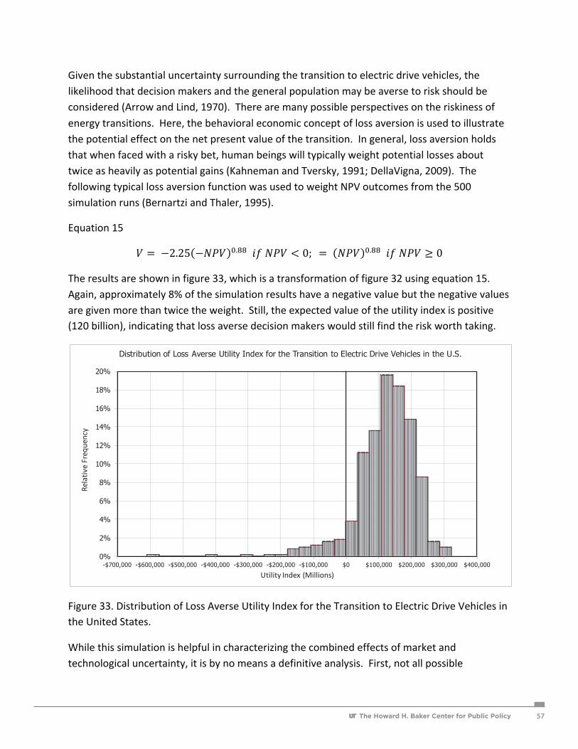
The Howard H. Baker Center for Public Policy The Howard H. Baker Center for Public Policy 57
Given the substantial uncertainty surrounding the transition to electric drive vehicles, the likelihood that decision makers and the general population may be averse to risk should be considered (Arrow and Lind, 1970). There are many possible perspectives on the riskiness of energy transitions. Here, the behavioral economic concept of loss aversion is used to illustrate the potential effect on the net present value of the transition. In general, loss aversion holds that when faced with a risky bet, human beings will typically weight potential losses about twice as heavily as potential gains (Kahneman and Tversky, 1991; DellaVigna, 2009). The following typical loss aversion function was used to weight NPV outcomes from the 500 simulation runs (Bernartzi and Thaler, 1995).
Equation 15
! = −2.25 −!"# !.!! !" !"# < 0; = !"# !.!! !" !"# ≥ 0
The results are shown in figure 33, which is a transformation of figure 32 using equation 15. Again, approximately 8% of the simulation results have a negative value but the negative values are given more than twice the weight. Still, the expected value of the utility index is positive (120 billion), indicating that loss averse decision makers would still find the risk worth taking.
Figure 33. Distribution of Loss Averse Utility Index for the Transition to Electric Drive Vehicles in the United States.
While this simulation is helpful in characterizing the combined effects of market and technological uncertainty, it is by no means a definitive analysis. First, not all possible
0%
2%
4%
6%
8%
10%
12%
14%
16%
18%
20%
-$700,000 -$600,000 -$500,000 -$400,000 -$300,000 -$200,000 -$100,000 $0 $100,000 $200,000 $300,000 $400,000
Relativ
e Frequency
Utility Index (Millions)
Distribution of Loss Averse Utility Index for the Transition to Electric Drive Vehicles in the U.S.

The Howard H. Baker Center for Public Policy58
technology paths are considered. In the simulation, technology trajectories vary greatly but they do not change direction. In reality, the cost of BEVs or FCVs, for example, could be constant for years and then suddenly change. The simulation does not allow for such a trajectory. Market preferences vary from iteration to iteration but do not change over time. In reality, preferences will change over time. Second, as pointed out above, policy makers do not change direction in the simulations. They force the Scenario 2 market shares regardless of the cost. In reality, policies would almost certainly adapt. If plug-‐in vehicles became very inexpensive relative to other options it is highly unlikely that policy makers would tax them to constrain their market shares to the levels of Scenario 2. If electric drive technologies costs did not decrease, policy makers would likely reduce losses by abandoning the transition before 2050. Both shortcomings will cause the distribution of simulation results to over-‐represent negative outcomes and under-‐represent positive ones. The question of how to model realistic, adaptive policy responses is left for future research.
VII. Inferences for Policymaking
The combined effects of long time constants, profound technological and market uncertainty, strong positive feedbacks via network externalities and other mechanisms, energy market deficiencies, and the central role of social costs make energy transitions an especially difficult problem for public policy. In addition, the current capacity to quantitatively analyze and model energy transformations is rudimentary. Many of the critical processes and parameters are not well understood and current models are either highly generalized or limited in scope. For this reason, results of the modeling should not be considered definitive. Even so, modeling and analysis can produce useful insights about the nature of the transition process and can help to broadly delineate the costs, benefits and uncertainties of transition.
As is true for any modeling analysis, premises are critical. This report has employed the model (LAVE-‐Trans) and technological and market assumptions of the NRC report, Transitions to Alternative Vehicles and Fuels (NRC, 2013). The NRC study’s premises were intended to be consistent with the goals of a 50% reduction in petroleum use by light-‐duty vehicles by 2030 and 80% reductions in greenhouse gas emissions and petroleum use by 2050. It assumed that GHG emissions and fuel economy standards will be continuously tightened through 2050. It further assumed that policies to promote the de-‐carbonization of fuels and the electricity sector will insure that low-‐carbon energy will be available to power transportation. It assumed that technological progress will gradually lower the long-‐run, high-‐volume costs of electric drive vehicles relative to internal combustion engine vehicles. All those assumptions have been retained.
For this study, the LAVE-‐Trans model was divided into two regions and re-‐calibrated: 1) California plus the Section 177 states that have opted into California’s vehicle emissions

The Howard H. Baker Center for Public Policy The Howard H. Baker Center for Public Policy 59
standards and ZEV program and, 2) the rest of the U.S. The analyses of timing and intensity of the ZEV mandates and the simulations illustrating uncertainty about technological progress and market conditions were based on Scenario 2 from the Phase I report (Greene et al., 2013a). Scenario 2 describes a successful transition to electric drive vehicles led by California and the states that have adopted California’s standards, and followed with a 5-‐year lag by the rest of the U.S. Automobile manufacturers were assumed to meet the ZEV mandates according to the ARB estimates of PHEV, BEV and FCV sales used in Scenario 2 of the Phase 1 report.
The Phase 1 analysis indicated that a transition to electric drive vehicles will require targeted policies, like ZEV mandates or equivalent subsidies together with infrastructure deployment, to accomplish the transition to electric drive vehicles. This will entail a decade or more of net subsidies by society. Subsidies could be paid by governments or the private sector (e.g., induced by regulation) or both. If electric drive technologies develop as anticipated by the NRC Transitions study, these policies can be phased out and ended by about 2030, leaving in place a sustainable transition to electric drive.
Given the NRC technology and market assumptions, the estimated benefits of the transition to electric drive are roughly an order of magnitude greater than the excess costs. Private benefits alone (energy savings and consumers’ surplus) are estimated to be several times the excess costs of the transition. However, a decade or more of net losses must be endured before benefits are likely to exceed costs. Private benefits (fuel savings, consumers’ surplus gains) and social benefits (reduced oil dependence and greenhouse gas emissions and improved air quality) are similar in magnitude. Assuming that the technology of electric drive vehicles does not improve significantly from its current status, as estimated by the NRC Transitions study, the total benefits of attempting a transition to electric drive are estimated to be roughly equal to the costs.
Delaying the ZEV mandates by five years or reducing their requirements is estimated to reduce the net present value of the transition. Using the NRC technology and market assumptions, the loss of benefits due to delaying or reducing the ZEV mandates is substantially greater than the savings in upfront costs. Even using pessimistic assumptions about the future costs of electric drive technologies there appears to be no net benefit to delaying or weakening the ZEV requirements.
Simulation of uncertainty about both technology and the market (using a 1-‐region, national version of the model) produced positive net present values in more than 90% of the iterations. The mean net present value was approximately $600 billion. The frequency of negative outcomes was less than 10% despite the fact that the simulation method tends to overestimate costs. However, 90% of the simulations showed annual losses through 2020, and it was not until 2025 that the expected annual values become positive. Transforming the distribution of

The Howard H. Baker Center for Public Policy60
outcomes to reflect loss aversion showed that a typically loss-‐averse decision maker would consider the transition to electric drive a risk worth taking.
The transition to electric-‐drive vehicles is a massive endeavor that requires special public policy initiatives beyond those normally required to address environmental problems. While it is highly beneficial in both the short and long run to internalize external costs, there is an additional need for temporary policies to overcome transition barriers by inducing positive feedback mechanisms. Vehicle subsidies or regulatory requirements and deployment of infrastructure are critical components of transition policy.22 Policies must be implemented in the face of substantial uncertainty as to their outcome and, thus, should be modified over time as knowledge is gained and circumstances change. Provided that electric drive technology progresses as the NRC “Transitions” report (NRC, 2013) anticipates, the temporary transition policies can be ended after a decade or so, leaving in place a self-‐sustaining electric drive vehicle market.
The risks of the transition to electric drive can be reduced by improving knowledge of transition barriers and processes, and by periodic reassessment and adaptation based on what has been learned. The limitations of current knowledge and analytical tools together with inherent uncertainty about future markets and technology imply that results of analyses such as this one should not be considered definitive. On the other hand, given the premises, assumptions and representation of uncertainty described in this report, it appears that the rewards of a transition to electric drive vehicles are likely to justify the cost of the effort several times over.
22 This report has focused on the economics of the transition. There are important social and institutional dimensions that must be addressed, as well. Codes and standards for new vehicular and energy systems and information about the new technologies are examples.

The Howard H. Baker Center for Public Policy The Howard H. Baker Center for Public Policy 61
VIII. References
1. Allcott, H. and M. Greenstone, 2012. “Is There an Energy Efficiency Gap?”, Working Paper 228, Energy Institute at Haas, University of California at Berkeley, January.
2. Arrow, K.J. and R.C. Lind, 1970. “Uncertainty and the Evaluation of Public Investment Decisions”, Economic Review, vol. 60, no. 3, pp. 364-‐378.
3. Arthur, W.B., 1990. “Positive Feedbacks in the Economy”, Scientific American, vol. 262, no. 2, pp. 92-‐99.
4. Bandivadekar, A., K. Bodek, L. Cheah, C. Evans, T. Groode, J. Heywood, E. Kasseris, M. Kromer and M. Weiss, 2008. On the Road in 2035, Laboratory for Energy and the Environment, Massachusetts Institute of Technology, Cambridge, MA.
5. Bastani, P., J.B. Heywood and C. Hope, 2012. “The effect of uncertainty on US transport-‐related GHG emissions and fuel consumption to 2050”, Transportation Research A, vol. 46, pp. 517-‐548.
6. Bernartzi, S. and R. Thaler, 1995. “Myopic Loss Aversion and the Equity Premium Puzzle”, Quarterly Journal of Economics, vol. 110, pp. 73-‐92.
7. Cabral, L.M.B., 1990. “On the Adoption of Innovations with Network Externalities”, Mathematical Social Sciences, vol. 19, pp. 299-‐308.
8. California Fuel Cell Partnership CAFCP), 2012. A California Road Map: The Commercialization of Hydrogen Fuel Cell Vehicles, West Sacramento, CA, June.
9. California Plug-‐In Electric Vehicle Collaborative (CAPEVC), 2010. Taking Charge: Establishing California Leadership in the Plug-‐In Electric Vehicle Marketplace, Plug-‐in Hybrid & Electric Vehicle Research Center, Institute of Transportation Studies, University of California at Davis.
10. Coase, R.H., 1960. “the Problem of Social Cost”, The Journal of Law and Economics, vol. III, pp. 1-‐44.
11. DellaVigna, S., 2009. “Psychology and economics: evidence from the field”, Journal of Economic Literature, vol. 47, no. 2, pp. 315-‐372.
12. Donndenlinger, J.A. and H.E. Cook, 1997. “Methods for Analyzing the Value of Automobiles”, SAE Technical Paper 970762, Society of Automotive Engineers, Warrendale, PA.
13. Element energy, 2011. “Influences on the Low Carbon Car Market from 2020-‐2030”, Final Report for the Low Carbon Vehicle Partnership, Cambridge, UK, July.
14. Energy Information Administration (EIA), 2011. Annual Energy Outlook 2011, DOE/EIA-‐0383(2011), U.S. Department of Energy, Washington, D.C.
15. Farrell, J. and P. Klemperer, 2007. “Coordination and Lock-‐in: Competition with Switching Costs and Network Effects”, Handbook of Industrial Organization, Volume 3, M. Armstrong and R. Porter, eds., Elsevier.

The Howard H. Baker Center for Public Policy62
16. Fawcett, A.A., K.V. Calvin, F.C. de la Chesnaye, J.M. Reilly and J.P. Weyant, 2009. “Overview of EMF 22 U.S. transition scenarios”, Energy Economics, vol. 31, pp. S198-‐S211.
17. Gallagher, K.S., A. Grübler, L. Kuhl, G. Nemet and C. Wilson, 2012. “The Energy Technology Innovation System”, Annual Review of Environment and Resources, pp. 137-‐162.
18. GEA, 2012: Global Energy Assessment -‐ Toward a Sustainable Future, Cambridge University Press, Cambridge, UK and New York, NY, USA and the International Institute for Applied Systems Analysis, Laxenburg, Austria.
19. Greene, D.L., C. Liu and S. Park, 2013a. Analyzing the Transition to Electric Drive in
California, White Paper 4.13, Howard H. Baker, Jr. Center for Public Policy, The University of Tennessee, Knoxville, TN, http://bakercenter.utk.edu/wp-‐content/uploads/2013/06/Transition-‐to-‐Electric-‐Drive-‐2013-‐report.FINAL_.pdf .
20. Greene, D.L., R.S. Lee and J.L. Hopson, 2013b. OPEC and the Costs to the U.S. Economy of Oil Dependence, White Paper 1-‐13, Howard H. Baker, Jr. Center for Public Policy, The University of Tennessee, Knoxville, TN, February.
21. Greene, D.L., D.H. Evans and J. Hiestand, 2013c. “Survey evidence on the willingness of U.S. consumers to pay for automotive fuel economy“, Energy Policy, vol. 61, pp. 1539-‐1550.
22. Greene, D.L. and K.G. Duleep, 2013d. Status and Prospects of the Global Automotive Fuel Cell Industry and Plans for Deployment of Fuel Cell Vehicles and Hydrogen Refueling Infrastructure, ORNL/TM-‐2013/222, Oak Ridge National Laboratory, Oak Ridge, Tennessee, June.
23. Greene, D.L., C. Liu and S. Park, 2012. “Light-‐duty Alternative Vehicle Energy Transitions (LAVE-‐Trans) Model: Working Documentation and User’s Guide”, Appendix H.2, Transitions to Alternative Vehicles and Fuels: Technical Appedixes, National Academies Press, Washington, D.C.
24. Greene, D.L. and S. Plotkin, 2011a. Reducing Greenhouse Gas Emissions from U.S. Transportation, Pew Center on Global Climate Change, Arlington, Virginia.
25. Greene, D.L., 2011b. “What’s Greener than a VMT Tax? The Case for an Indexed Energy User Fee to Finance U.S. Surface Transportation,” Transportation Research D-‐Environment, vol. 16, pp. 451-‐458.
26. Greene, D.L., 2011c. “Uncertainty, Loss Aversion and Markets for Energy Efficiency”, Energy Economics, vol. 33, pp. 608-‐616.
27. Greene, D.L., 2010. “Measuring Energy Sustainability: Making Progress,” in Linkages of Sustainability, T.E. Graedel and E. van der Voet, eds., Strüngmann Forum Reports, MIT Press, Cambridge, MA, 2010.

The Howard H. Baker Center for Public Policy The Howard H. Baker Center for Public Policy 63
28. Greene, D.L., 2001. TAFV Alternative Fuels and Vehicles Choice Model Documentation, ORNL/TM-‐2001/134, Oak Ridge National Laboratory, Oak Ridge, TN.
29. Greene, D.L., P.N. Leiby and Bowman, 2007. Integrated Analysis of Market Transformation Scenarios with HyTrans, ONRL/TM-‐2007/094, Oak Ridge National Laboratory, Oak Ridge, TN.
30. Groves, D.G. and R.J. Lempert, 2007. “A new analytic method for finding policy-‐relevant scenarios”, Global Environmental Change, vol. 17, pp. 73-‐85.
31. Grübler, A., N. Nakicenovic, D.G. Victor, 1999. “Dynamics of energy technologies and global change”, Energy Policy, vol. 27, pp. 247-‐280.
32. Interagency Working Group on Social Cost of Carbon (IWGSCC), United States Government, 2013. Technical Update of the Social Cost of Carbon for Regulatory Impact Analysis Under Executive Order 12866, May, 2013. Available at: http://www.whitehouse.gov/sites/default/files/omb/inforeg/social_cost_of_carbon_for_ria_2013_update.pdf .
33. Interagency Working Group on Social Cost of Carbon, United States Government, 2010. Technical Support Document: Social Cost of Carbon for Regulatory Impact Analysis
Under Executive Order 12866, February, 2010. Available at: http://www.epa.gov/otaq/climate/regulations/scc-‐tsd.pdf .
34. International Energy Agency (IEA), 2012. Energy Technology Perspectives 2012, OECD, Paris.
35. Jaffe, A.B. and R.N. Stavins, 1994. “The energy-‐efficiency gap”, Energy Policy, vol. 22, no. 10, pp. 804-‐810.
36. James, B. et al., “Manufacturing Cost Analysis of Fuel Cell Systems,” presentation at the 2011 U.S. DOE Hydrogen and Fuel Cells Program Annual Merit Review and Peer Evaluation, http://www.hydrogen.energy.gov/pdfs/review11/fc018_james_2011_o.pdf
37. James, B.D., J.A. Kalinoski and K.N. Baum, 2010. Mass Production Cost Estimation for Direct H2 PEM Fuel Cell Systems for Automotive Applications: 2010 Update, Directed Technologies, Inc., Arlington, Virginia.
38. Ji, S.G., C.R. Cherry, M.J. Bechle, Y. Wu and J.D. Marshall, 2012. “Electric Vehicles in China: Emissions and Health Impacts”, Environmental Science and Technology, vol. 46, no. 4, pp. 2018-‐2024.
39. Kahneman, D. and A. Tversky, 1991. “Choices, values and frames”, American Psychologist, vol. 39, pp. 341-‐350.
40. Katz, M.L. and C. Shapiro, 1994. “Systems Competition and Network Effects”, Journal of Economic Perspectives, vol. 8, no. 2, pp. 93-‐115.
41. Katz, M.L. and C. Shapiro, 1986. “Technology Adoption in the Presence of Network Externalities”, Journal of Political Economy, vol. 94, no. 4, pp. 822-‐841.

The Howard H. Baker Center for Public Policy64
42. Köhler, J., M. Grubb, D. Popp and O. Edenhofer, 2006. “The Transition to Endogenous Technical Change in Climate-‐Economy Models: A Technical Overview to the Innovation Modeling Comparison Project”, The Energy Journal, Special Issues on Endogenous Technological Change and the Economics of Atmospheric Stabilisation.
43. Kromer, M.A., J.B. Heywood, 2007. “Electric Powertrains: Opportunities and Challenges in the U.S. Light-‐Duty Vehicle Fleet, LFEE 2007-‐02 RP, Laboratory for Energy and the Environment, Massachusetts Institute of Technology, Cambridge, MA.
44. Lamberson, P.J. and S.E. Page, 2012. “Tipping Points”, SFI Working Paper 2012-‐02-‐002, Santa Fe Institute, http://www.santafe.edu/media/workingpapers/12-‐02-‐002.pdf , September 24, 2013.
45. Lave, C.A. and K. Train, 1979. “A Disaggregate Model of Auto-‐type Choice”, Transportation Research A, vol. 13A,pp. 1-‐9.
46. Lemoine, D.M. and C.P. Traeger, 2012. “Tipping Points and Ambiguity in the Economics of Climate Change”, Working Paper 18230, National Bureau of Economic Research, Cambridge, Massachusetts, July: http://www.nber.org/papers/w18230 (9/6/2013).
47. Lempert, R.J., D.G. Groves, S.W. Popper, and S.C. Bankes, 2006. “A General, Analytic Method for Generating Robust Strategies and Narrative Scenarios”, Management Science, vol. 52, pp. 514-‐528.
48. McCollum, D. and C. Yang, 2009. “Achieving deep reductions in US transport greenhouse gas emissions: Scenario analysis and policy implications”, Energy Policy, vol. 37, no. 12, pp. 5580-‐5596.
49. McKinsey and Company, 2011. A portfolio of powertrains for Europe: a fact-‐based analysis, The role of Battery Electric Vehicles, Plug-‐in Hybrids and Fuel Cell Electric Vehicles, available at http://ec.europa.eu/research/fch/pdf/a_portfolio_of_power_trains_for_europe_a_fact_based__analysis.pdf .
50. Michalek, J.J., M. Chester, P. Jaramillo, C. Samaras, C.S. Shiau, L. Lave, 2011. “Valuation of plug-‐in vehicle life-‐cycle air emissions and oil displacement benefits”, Proceedings of the National Academy of Sciences, Early Edition, approved July 26, 2011.
51. Nakićenović, N., A. Grübler and A. McDonald, 1998. Global Energy Perspectives, Cambridge University Press, Cambridge, UK.
52. National Highway Traffic Safety Administration (NHTSA), 2006. Vehicle Survivability and Travel Mileage Schedules, Technical Report DOT HS 809 952, National Center for Statistics and Analysis, U.S. Department of Transportation, Washington, D.C.
53. National Research Council (NRC), 2013. Transitions to Alternative Vehicles and Fuels, National Academies Press, Washington, D.C.

The Howard H. Baker Center for Public Policy The Howard H. Baker Center for Public Policy 65
54. National Research Council (NRC), 2009a. Transitions to Alternative Transportation Technologies —Plug-‐in Hybrid Electric Vehicles. The National Academies Press, Washington D.C.
55. National Research Council (NRC), 2009b. Hidden Costs of Energy: Unpriced Consequences of Energy Production and Use, National Academies Press, Washington, D.C.
56. National Research Council (NRC), 2008. Transitions to Alternative Transportation Technologies: A Focus on Hydrogen, Committee on Assessment of Resource Needs for Fuel Cell and Hydrogen Technologies, National Academies Press, Washington, D.C.
57. Office of Management and Budget (OMB), 2012. “Appendix C: Discount Rates for Cost-‐Effectiveness , Lease, Purchase, and Related Analyses”, OMB Circular No A-‐94, Memorandum from the Executive Office of the President of the United States, Washington, DC, January 3, 2012.
58. Ogden, J.M. and M. Nicholas, 2010. “Analysis of a “cluster” strategy for introducing hydrogen vehicles in Southern California”, Energy Policy, vol. 39, no. 4, pp. 1923-‐1938.
59. Page, W.H. and J.E. Lopatka, 1999. “Network Externalities”, Encyclopedia of Law and
Economics, 0760, B. Bouckaert and G. DeGeest, eds., Edward Elgar and University of Ghent, encyclo.findlaw.com/0760book.pdf .
60. Palisade Corporation, 2013. @Risk Version 6, Ithaca, NY, http://www.palisade.com/risk/ .
61. Sanstad, A.H., R.B. Howarth, 1994. “’Normal’ markets, market imperfections and energy efficiency”, Energy Policy, vol. 22, no. 10, pp. 811-‐818.
62. Shulock, C., E. Pike, A. Lloyd and R. Rose, 2011. Vehicle Electrification Policy Study, Task 1 Report: Technology Status, International Council on Clean Transportation, San Francisco, California.
63. Small, K.A. and H.S. Rosen. 1981. “Applied Welfare Economics with Discrete Choice Models,” Econometrica, vol. 49, no. 1, pp. 105-‐130, January.
64. Struben, J. and J.D. Sterman, 2008. “Transition challenges for alternative fuel vehicle and transportation systems”, Environment and Planning B: Planning and Design, vol. 35, pp. 1070-‐1097.
65. Tversky, A. and Kahneman, D., 1992. “Advances in prospect theory: cumulative representation of uncertainty”, Journal of Risk and Uncertainty, vol. 5, pp. 297-‐323.
66. U.S. Environmental Protection Agency and National Highway Traffic Safety Administration (EPA/NHTSA), 2011. Draft Joint Technical Support Document: Proposed Rulemaking for 2017-‐2025 Light-‐Duty Vehicle Greenhouse Gas Emission Standards and
Corporate Average Fuel Economy Standards, EPA-‐420-‐D-‐11-‐901, Washington, D.C., November.

The Howard H. Baker Center for Public Policy66
67. Weiss, M., M.K. Patel, M. Junginger, A. Perujo, P. Bonnel and G. van Grootveld, 2012. “On the electrification of road transport – Learning rates and price forecasts for hybrid-‐electric and battery-‐electric vehicles”, Energy Policy, http://dx.doi.org/10.1016/j.enpol.2012.05.038 .
68. Yang, C., D. McCollum and W. Leighty, 2011. “Scenarios for Deep Reductions in Greenhouse Gas Emissions”, Ch. 8 in J.M. Ogden and L. Anderson, eds., Sustainable Transportation Energy Pathways, Institute of Transportation Studies, University of California at Davis.
69. Zachmann, G., M. Holtermann, J. Radeke, M. Tam, M. Huberty, D. Naumenko, and A. Faye, 2012. The great transformation: decarbonising europe’s energy and transport systems, Bruegel Blueprint Series, vol. XVI, Bruegel, Brussels.
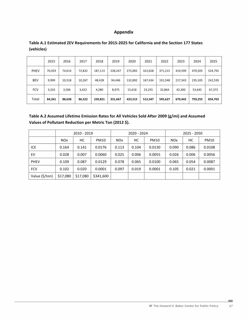
The Howard H. Baker Center for Public Policy The Howard H. Baker Center for Public Policy 67
Appendix
Table A.1 Estimated ZEV Requirements for 2015-‐2025 for California and the Section 177 States (vehicles)
2015 2016 2017 2018 2019 2020 2021 2022 2023 2024 2025
PHEV 70,929 74,614 72,832 187,113 228,247 275,005 322,658 371,215 419,599 470,505 524,792
BEV 9,999 10,518 10,267 48,428 94,446 132,892 167,434 191,548 217,543 235,105 242,539
FCV 3,333 3,506 3,422 4,280 8,975 15,618 23,255 32,864 42,300 53,645 67,372
Total 84,261 88,638 86,522 239,821 331,667 423,515 513,347 595,627 679,442 759,255 834,703
Table A.2 Assumed Lifetime Emission Rates for All Vehicles Sold After 2009 (g/mi) and Assumed
Values of Pollutant Reduction per Metric Ton (2012 $).
2010 -‐ 2019 2020 -‐ 2024 2025 -‐ 2050
NOx HC PM10 NOx HC PM10 NOx HC PM10
ICE 0.164 0.141 0.0176 0.113 0.104 0.0130 0.090 0.086 0.0108
EV 0.028 0.007 0.0060 0.025 0.006 0.0055 0.026 0.006 0.0056
PHEV 0.109 0.087 0.0129 0.078 0.065 0.0100 0.065 0.054 0.0087
FCV 0.102 0.020 0.0001 0.097 0.019 0.0001 0.105 0.021 0.0001
Value ($/ton) $17,080 $17,080 $341,600

The Howard H. Baker Center for Public Policy68
Table A.3 Probability Distributions for Market Response Parameters Used in Monte Carlo Simulation
Parameters Distribution
Min Mean Max
Importance of diversity of makes and models to choose from Triangle 0.50 0.67 1.00
Value of time ($/hr.) Triangle $10.00 $20.00 $40.00
Maximum value of public recharging to typical PHEV buyer Uniform $500 $1,000 $1,500
Cost of one day on which driving exceeds BEV range Uniform $10 $20 $30
Maximum value of public recharging to typical BEV buyer Uniform $0 $500 $1,000
Importance of fuel availability relative to standard assumption Triangle 0.67 1.00 1.67
Payback period for fuel costs (yrs.) Triangle 2.0 3.0 5.0 Volume threshold for introduction of new models rel. to std. assumptions Uniform 0.80 1.00 1.20
Optimal production scale relative to standard assumptions Uniform 0.75 1.00 1.25
Scale elasticity relative to standard assumptions Uniform 0.50 1.00 1.50
Progress Ratio relative to standard assumptions Uniform 0.96 1.00 1.04
Price elasticities of vehicle choice relative to standard assumptions Uniform 0.60 1.20 1.80
Percentage of new car buyers who are innovators Triangle 5.0% 15.0% 20.0%
Willingness of innovators to pay for novel technology ($/mo.) Uniform $100 $200 $300
Cumulative production at which innovators WTP is reduced by 1/2 Uniform 500,000 1,000,000 1,500,000
Majority's aversion to risk of new technology ($/mo.) Uniform -$900 -$600 -$300
Cumulative production at which majority's risk is reduced by 1/2 Uniform 500,000 1,000,000 1,500,000
Fraction of +/- 20% deviation from Mid-Range price path (5 γ’s) Triangular -1.0 0.0 1.0
Recommended