Louisiana State UniversityLSU Digital Commons
LSU Historical Dissertations and Theses Graduate School
1994
Traction and Agricultural Tractor Tire SelectionStudies.Francois Pascal BrassartLouisiana State University and Agricultural & Mechanical College
Follow this and additional works at: https://digitalcommons.lsu.edu/gradschool_disstheses
This Dissertation is brought to you for free and open access by the Graduate School at LSU Digital Commons. It has been accepted for inclusion inLSU Historical Dissertations and Theses by an authorized administrator of LSU Digital Commons. For more information, please [email protected].
Recommended CitationBrassart, Francois Pascal, "Traction and Agricultural Tractor Tire Selection Studies." (1994). LSU Historical Dissertations and Theses.5855.https://digitalcommons.lsu.edu/gradschool_disstheses/5855

INFORMATION TO USERS
This manuscript has been reproduced from the microfilm master. UMI films the text directly from the original or copy submitted. Thus, some thesis and dissertation copies are in typewriter face, while others may be from aity type of computer printer.
The quality of this reproduction is dependent upon the quality of the copy submitted. Broken or indistinct print, colored or poor quality illustrations and photographs, print bleedthrough, substandard margins, and improper alignment can adversely afreet reproductioiL
In the unlikely event that the author did not send UMI a complete manuscript and there are missing pages, these will be noted. Also, if unauthorized copyright material had to be removed, a note wül indicate the deletion.
Oversize materials (e.g., maps, drawings, charts) are reproduced by sectioning the original, beginning at the upper left-hand comer and continuing from left to right in equal sections with small overlaps. Each original is also photographed in one exposure and is included in reduced form at the back of the book.
Photogr^hs included in the original manuscript have been reproduced xerograpMcaUy in this copy. Higher quality 6" x 9" black and white photographic prints are available for any photographs or illustrations appearing in this copy for an additional charge. Contact UMI directly to order.
UMIA Bell & Howell Information Com pany
300 North Z eeb Road. Ann Arbor. Ml 48106-1346 USA 313.'761-4700 800/521-0000
R eproduced with perm ission of the copyright owner. Further reproduction prohibited without perm ission.

R e p ro d u c e d with perm iss ion of th e copyright ow ner. F u r th e r reproduction prohibited without perm iss ion .

TRACTION AND AGRICULTURAL TRACTOR TIRE SELECTION STUDIES
A Dissertation
Submitted to the Graduate Faculty of the Louisiana State University and
Agricultural and Mechanical College in partial fulfillment of the
requirements for the degree of Doctor of Philosophy
in
The Interdepartmental Progi-ams in Engineering
byFrançois Pascal B rassart
Diplôme d’ingénieur de l’Ecole Nationale Supérieure d’Arts et Métiers, Paris, France, 1987
M.S. in Ag.E., Louisiana State University, 1989 December 1994
R eproduced with perm ission of the copyright owner. Further reproduction prohibited without perm ission.

UMI Number: 9524434
ÜMI Microform Edition 9524434 Copyright 1995, by OMI Company. All rights reserved.
This microform edition is protected against unauthorized copying under Title 17, United States Code.
u300 North Zeeb Road Ann Arbor, MI 48103
R eproduced with perm ission of the copyright owner. Further reproduction prohibited without perm ission.

ACKNOWLEDGMENTS
The author would like to express his appreciation to his major professor,
Dr. Malcolm E. Wright, for his support, advice and encouragement during
the course of the work.
Thanks also goes to the Pirelli-Armstrong Tire Company for providing
tires with the friendly advice and impetus of Ron Rode, to the Case IH
Company for funding this project, and to the personnel of the United States
Department of Agriculture, Agriculture Research Service (USDA-ARS),
National Soil Dynamics Laboratory (NSDL), Auburn, Alabama, for helping
in performing some of the experiments presented here, especially
Agricultural Engineer Thomas R. Way. The active and friendly
participation of the NSDL personnel in discussing the experimental design
and in making the traction experiments largely contributed to the
achievement of this project.
The author would also like to thank all the staff members and students
of the Department of Biological and Agricultural Engineering at Louisiana
State University for their help, friendliness and understanding during his
stay at LSU. Special appreciation goes to all the friends the author has
made, and those he has left in France while being at LSU. Finally, great
thanks goes the author’s family for their constant support during his
studying a t LSU.
11
R eproduced with perm ission of the copyright owner. Further reproduction prohibited without perm ission.

TABLE OF CONTENTS
ACKNOWLEDGMENTS ......................................................................................... ii
LIST OF TABLES ................................................................................................ Wi
LIST OF FIGURES ................................................................................................ x
ABSTRACT ............................................................................................................... xiv
INTRODUCTION ..................................................................................................... 1Problem S ta tem ent .............................................................................................. 1Objective .................................................................................................................. 2General Approach ................................................................................................ 3
LITERATURE REVIEW ......................................................................................... 6Tire and Traction Terminology' ....................................................................... 6
Tire Definitions ................................................................................................ 6Tire Designation .............................................................................................. 9Wheel Mechanics and Traction Terminology ........................................ 12Tractor Mechanics ...................................................................................... 17
Force Analysis ........................................................................................... 19Power Analysis ......................................................................................... 24Other Performance Criteria ................................................................... 30
Tire Mechanical Properties ............................................................................ 33Rolling Radius on a Rigid Surface ........................................................... 33
Charles and Schuring Rolling Radius Model ................................... 33Clark Rolling Radius Model .................................................................. 36Brixius and Wismer Rolling Radius Alodel ....................................... 36
Static Deflection, Stiffness and Contact Area on Rigid Surface . . . . 37Dynamic Stiffness and Damping Studies ............................................... 44Effect of Inflation Pressure ....................................................................... 55
Traction and Power Measurements ........................................................... 60Experimental Procedures ............................................................................ 61Test Track M easurements .......................................................................... 64Field and Soil Bin Measurements ........................................................... 65Indoor M easurem ents ................................................................................. 70
Traction Prediction ........................................................................................... 74Preliminary Work by Freitag ..................................................................... 74Traction on Concrete .................................................................................... 78Traction in the Field .................................................................................... 81
Zoz Traction Prediction Chart .............................................................. 81Wismer and Luth Traction Model ...................................................... 81
iii
R eproduced with perm ission of the copyright owner. Further reproduction prohibited without perm ission.

Gee-Clough Traction Model ................................................................... 83Brixius Traction Model .......................................................................... 85Other Traction Models ............................................................................ 88
Computer Simulation and Decision Aids ............................................... 96Soil Behavior and Soil-Tire Interactions ......................................................107
Wheel Sinkage and Soil Deformation ......................................................108Soil Properties Related to Traction ...........................................................113
Friction and Cohesion .............................................................................. 113Soil S trength ............................................................................................... 114
Soil Stress Distribution Under a Point Load ......................................... 117Effect of a Vertical Point Load ................................................................118Effect of a Horizontal Point Load ...........................................................120Stress Distribution in Agricultural Soils ............................................121
Stresses Under Distributed Loads ............................................................. 124Integration Methods .................................................................................124Superposition Methods ............................................................................125Finite Elements Method ......................................................................... 125Other Soil Stress and Deformation Prediction Methods ................... 129
Stress Distribution Under Rigid Wheels .................................................129Stress Distribution Under Tires ................................................................131
Load Distribution Models .......................................................................132Integrated Tools and Combined Methods ............................................136
Soil-Wheel Contact Stresses .......................................................................137Traction Model Based on Soil-Wheel Contact Stresses ........................ 141Experimental Traction Results .................................................................... 144
EXPERIMENTAL SETUP AND EXPERIMENT DESCRIPTION ............148Static Measurements .......................................................................................... 148
Apparatus for Static Experiments ............................................................. 148Static Experiment Description .................................................................... 153Data Collected ..................................................................................................155Tests to Evaluate Measurement Error ......................................................159
Instrum entation Settlement and Drift .................................................159Variations Ajnong Identical Tests ...........................................................161Variations Within One Tire Lug Pitch .................................................162Variations Around the Tire Circumference ......................................... 163
Dynamic Measurements ...................................................................................166Apparatus for Dynamic Experiments ........................................................ 166
Determination of and C j .................................................................... 168Second Determination Method ............................................................... 169
Dynamic Experiment Description ............................................................... 177Data Collected ..................................................................................................178
Traction Measurements ..................................................................................... 179Traction Apparatus ........................................................................................179
IV
R eproduced with perm ission of the copyright owner. Further reproduction prohibited without perm ission.

Traction Experiment Description ................................................................ 189Traction Data Collected ................................................................................. 201
RESULTS AND DISCUSSION ............................................................................ 203Static Experiments ..............................................................................................203
Comparison Between Same-Size Tires ......................................................206Bias Versus Radial Construction C o m p a r is o n ..........................................207Comparison Between Tires of Different Width .......................................208
Dynamic Experiments .........................................................................................208Comparison Between Same-Size T i r e s ........................................................ 213Bias Versus Radial Construction C o m p a r is o n ..........................................214Comparison Between Tires of Different Width ....................................... 215
Traction Experiments .........................................................................................219Rolling Radius .................................................................................................. 224Gross and Net Traction Versus Dynamic Load ....................................... 229
SUMMARY AND CONCLUSIONS .....................................................................238Summary ...............................................................................................................238Conclusions ............................................................................................................ 241
REFERENCES ....................................................................................................... 243
APPENDIX A: TIRE AND TRACTION VARIABLES .................................. 265
APPENDIX B: MANUFACTURER DATA FOR SENSORS USEDON LSU TIRE-LOADING MACHINE ............................................................. 276
Load Cells ...............................................................................................................276M anufacturer Data .........................................................................................276Calibration Cuiwes ........................................................................................... 276
Linear Displacement Transducer .....................................................................279Manufacturer Data .........................................................................................279Calibration Curve ...........................................................................................279
Inflation Pressure Gage ...................................................................................... 280
APPENDIX C: TIRE AND TUBE DATA ...........................................................282
APPENDIX D: SAMPLE STATIC LOAD-DEFLECTION DATA .............. 286
APPENDIX E: PROGRAIM ECC2.F0R AND 8M IP L E RESULTS ............288Program ECC2.F0R ........................................................................................... 288Sample Results .....................................................................................................293
APPENDIX F: SAIVIPLE D^^-NAAIIC LOAD-DEFLECTION DATA ____ 295
R eproduced with perm ission of the copyright owner. Further reproduction prohibited without perm ission.

APPENDIX G: SAMPLE CONE INDEX, ROLLING RADIUS AND TRACTION DATA .................................................................................................. 297
APPENDIX H; LOTUS 1-2-3 SPREADSHEET PROGRAMSUSED TO TREAT LSU AND NSDL DATA ................................................... 303
Static Load-Deflection Data .............................................................................. 303Dynamic Load-Deflection Data ....................................................................... 303Cone Index D ata .................................................................................................. 304Rolling Radius Data ...........................................................................................305Traction Data ....................................................................................................... 305
APPENDIX I: SAS PROGRAM AND OUTPUTS ............................................307SAS Program Including Data ..........................................................................307GLM Outputs and Least-Square Means According to Tire Width . . . . 309 GLM Outputs and Least-Square Means According to Carcass Construction ........................................................................................ 314
VITA ...........................................................................................................................321
VI
R eproduced with perm ission of the copyright owner. Further reproduction prohibited without perm ission.

LIST OF TABLES
1 Values of k for Four Tractor Tires, Measured at ZeroDrawbar Pull (Charles and Schuring, 1984) 34
2 Stiffness and Damping Characteristics of Tires asMeasured by Janssen and Schuring (1985) ........................................ 48
3 Stiffnesses and Damping Coefficients Used by Crolla,Horton, and Stayner (1990) ..................................................................... 53
4 Coefficients of Traction Obtained by Taylor andWilliams (1958) 71
5 Equations for Traction on Outdoor Tracks (Goupillonand Hugo, 1988) ......................................................................................... 72
6 Dimensions of Treadless Tires Used by Freitag (1966)for Dimensional Analysis ........................................................................ 74
7 Independent Tire-Soil System Variables Used by Freitag (1966) . 75
8 Dependent Variables Used by Freitag ................................................... 75
9 Typical Wheel Numeric Values (from ASAE Standard D230.4) . . 82
10 Range of Field Test Variables Used by Brixius (1987) ..................... 87
11 Coefficients Used by Al-Hamed et al. (1990) in BrixiusTraction Model ........................................................................................... 99
12 Estimates of Cone Index According to Soil Conditions ....................... 101
13 Estimates of Optimum Slip According to Tractor DriveType and Soil ................................................................................................ 101
14 Optimum Slip Ranges for Maximum TE According toSoil Type (ASAE Standard EP391.1) ...................................................... 102
15 Draft Estimates According to Implement Tcqje ...................................10 0
16 Ratio of Drawbar Power to PTO Power According toSoil Condition and Tractor Drive Type ................................................. 103
V I 1
R eproduced with perm ission of the copyright owner. Further reproduction prohibited without perm ission.

17 Typical Cone Index Values (Brixius, 1987) 116
18 Inverses of Rolling Radius Versus Dynamic Load,M easured on Concrete ............................................................................... 196
19 Test Plot Locations for the First Soil Bin Preparation,Norfolk Sandy Loam, V-\VheeI Packed, Surface LeveledWith Scraper Blade .................................................................................... 198
20 Test Plot Locations for the Second Soil Bin Preparation,Norfolk Sandy Loam, V-Wheel Packed, Surface LeveledW ith Scraper Blade .................................................................................... 199
21 Average Value, Standard Deviation and Coefficient ofVariation of Cone Index and Tip Speed ................................................. 201
22 Linear Regression Coefficients for Static StiffnessVersus Inflation Pressure Curves ........................................................... 205
23 Computed Static Stiffness a t Various Inflation Pressures ................ 206
24 Linear Regression Coefficients for the Dynamic Stiffness andDamping Coefficient Versus Inflation Pressure Curves ................... 209
25 Ratios of Dynamic Stiffness to Static Stiffness .................................... 210
26 Computed Dynamic Stiffness a t Various Inflation Pressures . . . . 212
27 Computed Damping Coefficient a t Various Inflation Pressures . . 213
28 Values of a t 41 and 124 kPa Inflation Pressure for30-Inch Rim Tires .........................................................................................216
29 Values of a t 41 and 110 kPa Inflation Pressure for38-Inch Rim Tires .........................................................................................216
30 Variations of Inflation Pressure, Actual Speed, AngularVelocity and Slip During Tests of Tires #2 and #3 ............................. 222
31 Variations of Inflation Pressure, Actual Speed, AngularVelocity and Slip During Tests of Tires #17 and #20 ....................... 223
32 Regression Coefficients for Rolling Radius as a Functionof Dynamic Load and Inflation Pressure ...............................................229
vui
R eproduced with perm ission of the copyright owner. Further reproduction prohibited without perm ission.

33 Levels of Significance of Replication, Construction, InflationPressure, Slip, and Their Combinations on Traction Ratios ............232
34 Levels of Significance of Replication, Tire Width, InflationPressure, Slip, and Their Combinations on Traction Ratios ............233
A Tire and Traction Variables ...................................................................... 265
C l Tire-Tube Matching Table ...........................................................................282
C2 Tire D ata (After Armstrong M aster Dealer Price List 6090 and"Tirebrochure" Computer Program) ........................................................ 284
C3 Rated tire Loads (After Tire and Rim Association, 1989, andArmstrong Tire Load Calculation Equations) .....................................285
D1 Spreadsheet File Containing Static Load-Deflection Data ............... 286
D2 Ranges of Inflation Pressure and Number of Tests PerformedUnder Static Conditions for Each Tire ................................................. 287
F I Spreadsheet File Containing Dynamic Load-Deflection Data . . . . 295
F2 Ranges of Inflation Pressure and Number of Tests PerformedUnder Dynamic Conditions for Each Tire ............................................296
G l A Spreadsheet File Containing Rolling Radius Data .........................298
G2 Location and Filenames of Cone Index MeasurementsBefore Traffic for the First Soil Bin Preparation,Norfolk Sandy Loam, V-Wheel Packed, Surface LeveledWith Scraper Blade ....................................................................................299
G3 Location and Filenames of Cone Index MeasurementsBefore Traffic for the Second Soil Bin Preparation,Norfolk Sandy Loam, V-Wheel Packed, Surface LeveledWith Scraper Blade ....................................................................................300
G4 A Spreadsheet File Containing Traction Data ..................................... 301
G5 A Spreadsheet File Containing Traction Data ..................................... 302
IX
R eproduced with perm ission of the copyright owner. Further reproduction prohibited without perm ission.

LIST OF FIGURES
1 Dimensions of a tire ...................................................................................... 6
2 Types of tire carcass construction (Michelin, 1988) .............................. 9
3 Forces acting on a driven wheel ............................................................ 13
4 Main types of tractor drive configurations ......................................... 18
5 Forces acting on a stationary t r a c t o r ..................................................... 20
6 Forces acting on a foiu’-wheel drive tractor understeady-state conditions ............................................................................. 22
7 Typical power transmission efficiencies for tractorshaving gear-type transmissions .............................................................. 29
8 Examples of available drawbar power values on varioussurfaces for a tractor rated a t 116 HP (engine horsepower) .......... 29
9 Different wheel radii used by Charles and Schuring (1984) ............. 35
10 Tire dimensions used by Upadhyaya and Wulfsohn(1990) in tire deflection and contact area mode! .............................. 41
11 Schematic of the NIAE single wheel tester ......................................... 67
12 Schematic of the University of California single wheel tester . . . 68
13 Schematic of the University of Oklahoma single wheel tester . . . 69
14 Limits of traction prediction equations for the Brixius model . . . 87
15 Soil deformation under pneumatic wheels (Kdiamidov, 1961) . . . . 110
16 Bekker pressure-sinkage curve ................................................................. I l l
17 Cohesive and frictional characteristics of soils ...................................... 115
18 Soil stress coordinate system ....................................................................118
R eproduced with perm ission of the copyright owner. Further reproduction prohibited without perm ission.

19 Force equilibrium of a powered wheel (Wulfsohn mrdUpadhyaya, 1991) ........................................................................................ 142
20 CAD drawing of the LSU tire-loading machine .................................... 150
21 General view of the LSU tire-loading machine ....................................151
22 Schematic of a static tire-loading experiment ...................................... 154
23 Tire sizes used in static and dynamic experiments ............................ 156
24 Deflection versus load curve, 15.5-38 tire #13 at 138 kPainflation pressure ........................................................................................ 158
25 Settlement and drift of the data logging systemin static conditions ......................................................................................160
26 Variations among similar stiffness measurementsfor 4 levels of inflation pressure (15.5-38 tire # 1 3 ) ............................. 162
27 Variations of stiffness along one pitch lengthfor 4 levels of inflation pressure (15.5-38 tire # 1 3 ) ............................. 163
28 Variations of stiffness around the tire circumferencefor 4 levels of inflation pressure (15.5-38 tire # 1 3 ) ............................. 164
29 Coefficients of variability for stiffness measurements ....................... 165
30 Spring-and-damper model of a tire ......................................................... 166
31 Force and deflection versus time, theoretical parallel spring-and-damper system (I\,,.„ - 504.5 kN/m,Cj = 16 .8skN /m ) ..................' ....................................................................168
32 Theoretical tire dynamic load versus harmonic deflectioncycle (Kjy„ = 504.5 kN/m, Cj = 16.8 s kN/m) ....................................... 170
33 Actual tire dynamic load versus harmonic deflection cycle(14.9R30 tire #3 at 207 kPa inflation pressure) .................................. 170
34 Measured and computed load and deflection versus time(14.9R30 tire #3 at 207 kPa inflation pressure) .................................. 172
35 Geometry of an eccentric mechanism .................................................... 173
XI
R eproduced with perm ission of the copyright owner. Further reproduction prohibited without perm ission.

36 Length adjustm ent on the rod of the eccentric mechanism ..............176
37 Schematic of a dynamic tire loading experiment ..................................178
38 Composition of Norfolk Sandy Loam ........................................................ 181
39 NSDL rotary tiller car ................................................................................ 182
40 NSDL scraper blade car ..............................................................................182
41 Packing elements of the NSDL V-wheel packer ....................................184
42 NSDL single-wheel tester and instrumentation cars ..........................184
43 Schematic of the NSDL single-wheel tester ........................................... 185
44 Cone index versus depth curve, Norfolk Sandy Loam,V-wheel packed, surface leveled with scraper blade ...........................200
45 Tire static stiffness versus inflation pressure curvefor 14.9R30 tire #3 204
46 Tire dymamic stiffness and damping coefficient versusinflation pressure curves for 14.9R30 tire #3 ....................................... 209
47 Rolling radius versus dynamic load, 14.9-30 tire #2 a t 83 kPa inflation pressure .........................................................................................224
48 Twenty-point averages of rolling radius versus dynamic load,14.9-30 tire #2 at 83 kPa inflation p r e s s u r e ..........................................225
49 Computed rolling radius versus load of 14.9-30 tire #2at various inflation pressures .................................................................. 226
50 Computed rolling radius versus load of 14.9R30 tire #3at various inflation pressures .................................................................. 226
51 Computed rolling radius versus load of 18.4-38 tire #17 a t various inflation pressures ............................................. 227
52 Computed rolling radius versus load of 1S.4R3S tire #20at various inflation pressures .................................................................. 227
Xll
R eproduced witfi perm ission of tfie copyrigfit owner. Furtfier reproduction profiibited witfiout perm ission.
53 Gross and net traction versus d^Tiamic load, 14.9-30tire #2 a t 15% slip ...................................................................................... 230
54 Twenty-point averages of gross and net traction versusdynamic load, 14.9-30 tire #2 a t 15% slip ............................................ 230
55 Least-square means of gross pull ratio and net pull ratio versusinflation pressure and slip for 14.9-30 tire #2 234
56 Least-square means of gross pull ratio and net pull ratio versusinflation pressure and slip for 14.9R30 tire #3 235
56 Least-square means of gross pull ratio and net pull ratio versusinflation pressure and slip for 18.4-38 tire #17 235
56 Least-square means of gross pull ratio and net pull ratio versusinflation pressure and slip for 18.4R38 tire #20 ................................. 236
B1 Calibration curve for load cell #1 277
B2 Calibration curve for load cell #2 278
B3 Calibration curve for load cell #3 278
B4 Calibration curve for the displacement transducer ........................... 280
B5 Calibration curve for the inflation pressure gage .................................281
xin
R eproduced with perm ission of the copyright owner. Further reproduction prohibited without perm ission.

ABSTRACT
A machine was built to study non-rolling tire stiffness and damping
coefficients of agricultural tractor tires in the vertical direction. Static
deflection on a rigid surface was measured as a function of vertical load.
During dynamic experiments, a sinusoidal forcing function was imposed on
the test tire to determine dynamic stiffness and damping coefficient from
load and deflection measurements. The experimental setup and
methodology are described. Ten tires were tested. Both static and dynamic
stiffnesses appeared linearly related to inflation pressure. No correlation
was found between dynamic properties and excitation frequency.
Comparisons among stiffness and damping coefficient values were made
according to section width, carcass construction, and between tires of the
same size. Traction tests were made a t the National Soil Dynamics
Laboratory, Auburn, Alabama. Four tires (14.9-30, 14.9R30, 18.4-38 and
18.4R38) were tested on Norfolk Sandy Loam after measuring their rolling
radius on concrete under self-propelled condition, at three levels of inflation
pressure, and under varying load. Traction experiments were made at three
levels of inflation pressure, two levels of longitudinal slip (7.5 and 15% j and
under varying dynamic load for each tire. Slip, carcass construction and
inflation pressure significantly affected the pull ratios. A mathematical
model is proposed tha t accounts for effects of tire inflation pressure and
d}Tiamic load on rolling radius.
xiv
R eproduced with perm ission of the copyright owner. Further reproduction prohibited without perm ission.

INTRODUCTION
Problem Statement
Extensive research is done throughout the World to design and improve
tires, bu t little is known in the public domain about their mechanical
properties and physical behavior. Recent developments in the design of
agricultural tractors, and off-road vehicles in general, and the increasing
concerns about energy savings, soil conservation and safety have underlined
the need for extending the general knowledge and understanding of
agricultural tire behavior. Alcock (1986) listed the functions to be
performed by tractor tires as follows:
1. Support the tractor and associated loads at some low level of
ground pressure;
2. Absorb shock loads and cushion the vehicle against minor surface
irregularities;
3. Provide traction (and braking);
4. Provide for steering and directional stability;
5. Resist the abrasive action of the various surfaces.
In 1987, 1.07 million rear tractor tires were sold in the U.S. domestic
market. Of these tires, 74% were replacements and 79% were of the
general purpose, rear tractor tire type (called R-1), the most common being
the 18.4x38 size, with a unit price of about $670. Of the 980,000 front
1
R eproduced with perm ission of the copyright owner. Further reproduction prohibited without perm ission.
tractor tires sold within the same year, 93% were replacements and 85%
were of the general farming, dual or triple rib type (called F-2). The most
popular front size was the 6.00x16 priced at about $50. Rear tractor tires
are replaced on an average of every 3 years (Rode, 1989).
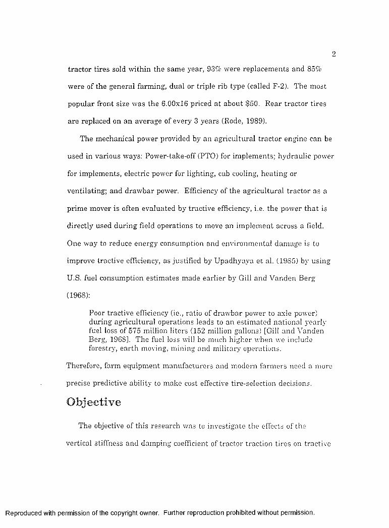
The mechanical power provided by an agricultural tractor engine can be
used in various ways; Power-take-off (PTO) for implements; hydraulic power
for implements, electric power for lighting, cab cooling, heating or
ventilating; and drawbar power. Efficiency of the agricultural tractor as a
prime mover is often evaluated by tractive efficiency, i.e. the power th a t is
directly used during field operations to move an implement across a field.
One way to reduce energy consumption and environmental damage is to
improve tractive efficiency, as justified by Upadhyaya et al. (1985) by using
U.S. fuel consumption estimates made earlier by Gill and Vanden Berg
(1968):
Poor tractive efficiency (ie., ratio of drawbar power to axle power) during agricultural operations leads to an estimated national yearly fuel loss of 575 million liters (152 million gallons) [Gill and Vanden Berg, 1968]. The fuel loss will be much higher when we include forestry, earth moving, mining and military operations.
Therefore, farm equipment manufacturers and modern farmers need a more
precise predictive ability to make cost effective tire-selection decisions.
The objective of this research was to investigate the effects of the
vertical stiffness and damping coefficient of tractor traction tires on tractive
R eproduced with perm ission of the copyright owner. Further reproduction prohibited without perm ission.

3
performance, and improve on existing techniques used to estimate the
performance of tractor/tire combinations.
General Approach
A research program was started at Louisiana State University (LSU) to
a ttem pt to fulfill the objective. This program included both laboratory and
field experiments to determine relationships between agricultural tire
mechanical properties, i.e. stiffness and damping characteristics, and
traction characteristics. A special machine was designed and built for the
laboratory experiments. It was used to determine the vertical stiffness of
tires under static conditions, and both vertical stiffness and damping
coefficient under dynamic conditions. Field experiments were performed at
the National Soil Dynamics Laboratoi-y (NSDL), Auburn, Alabama, where
state-of-the-art equipment to measure tire tractive performance in a
controlled environment was available (specially designed soil bins and
machinery).
Traction is affected by several parameters related to the soil, the
implement, the tractor, and its tires.
Factors related to the soil are:
Soil mechanical conditions (strength, state of compaction),
Soil physical conditions (structure, moisture content);
Factors related to the implement are:
R eproduced with perm ission of the copyright owner. Further reproduction prohibited without perm ission.

4
Forces transm itted by the implement to the tractor due to the actions
of the soil on the implement,
Forces transm itted by the implement to the tractor due to implement
weight or inertia;
Factors related to the tractor are:
Available power a t the driving axle(s),
Weight of the tractor on the axles,
Dimensions of the tractor;
Factors related to the tires are:
Carcass construction.
Inflation pressure,
Dimensions of the tires,
Number of tires.
Location of the tires.
Travel speed is also known to affect traction, but to a less significant extent,
within the range of operating conditions commonly encountered.
Metric units have been used as much as possible in this work, but other
units may appear for various reasons, such as quotations from other
researchers and designations based on English units in use throughout the
tire industry. For example, inches were used as the unit for tire width and
rim diameter because tire designations are based on this unit, even in
countries where metric units are used.
R eproduced with perm ission of the copyright owner. Further reproduction prohibited without perm ission.

5
The discussion was restricted to wheeled tractors because they are the
most used prime movers in agriculture. However, all the definitions and
equations presented below could be applied to other off-road, wheeled
vehicles, such as combines, self-propelled harvesters, etc.
R eproduced with perm ission of the copyright owner. Further reproduction prohibited without perm ission.

LITERATURE REVIEW
Tire and Traction Terminology
T ire D efin itio n s
Most of the definitions presented below were taken from, or derived
from American Society of Agricultural Engineers (ASAE) Standard S296.3
(1989a). F ig u re 1 shows the tire dimensions defined below.
no loadunloaded section height
rundiam eter
unloaded section width -
W-rfdeflection
loadedradius
load
loadedsectionwidth
F igure 1. D im ensions o f a tire.
T ire o v e ra l l d ia m e te r (d): T i re c i rc u m fe re n c e (C) measured over the
lugs, in the center plane, divided by k, with the tire mounted on its
R eproduced with perm ission of the copyright owner. Further reproduction prohibited without perm ission.

7
recommended rim and inflated to recommended operating pressure in an
unloaded condition.
d = - (1)TC
U n lo a d e d s t a t i o n a r y t i r e r a d iu s (r^):
= I « )
S ta t ic lo a d e d t i r e r a d iu s (r^): Distance from the center of the axle to the
supporting surface for a tire when inflated to recommended pressure,
mounted on an approved rim and carrying the recommended load.
Recommendations for inflation pressures, rims and loads are given by tire
manufacturers, the Tire and Rim Association, etc.
S t a t io n a r y t i r e d e f le c t io n (6): Difference between unloaded and loaded
stationary tire radii.
à = (3)
U n lo a d e d t i r e s e c t io n w id th (b„): The width of a new tire, including
normal growth caused by inflation and including normal side walls but not
including protective side ribs, bars, or decorations.
U n lo a d e d t i r e o v e ra l l w id th : The width of a new tire, including normal
growth caused by inflation, and including protective side ribs, and
decorations.
T r e a d w id th Distance from shoulder to shoulder (chord or arc).
R eproduced with perm ission of the copyright owner. Further reproduction prohibited without perm ission.
8
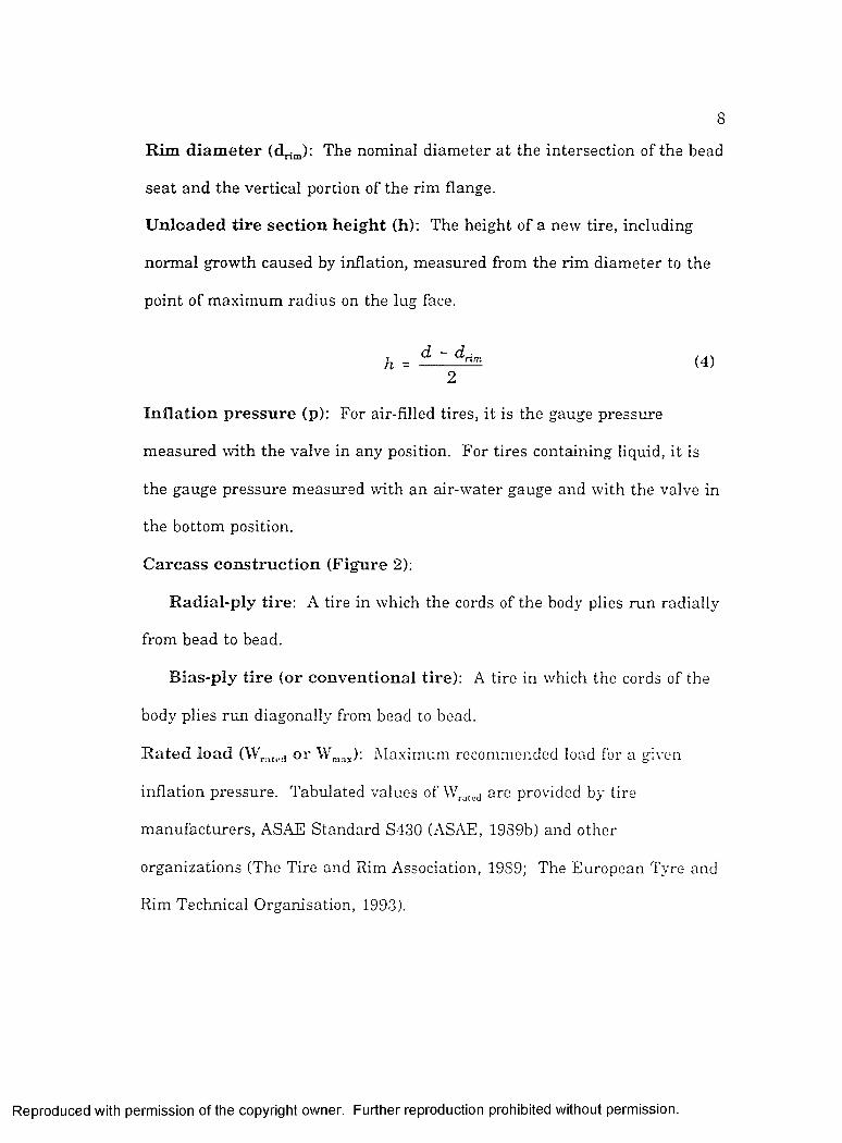
Rim diam eter (d^nj): The nominal diameter a t the intersection of the bead
seat and the vertical portion of the rim flange.
Unloaded tire section height (h): The height of a new tire, including
normal growth caused by inflation, measured from the rim diam eter to the
point of maximum radius on the lug face.
h = - - ..7 ^1'" (4)2
In f la t io n p r e s s u r e (p): For air-filled tires, it is the gauge pressure
measured with the valve in any position. For tires containing liquid, it is
the gauge pressure measured with an air-water gauge and with the valve in
the bottom position.
C a rc a s s c o n s t r u c t io n (F ig u re 2);
R ad ia l-p ly tire : A tire in which the cords of the body plies run radially
from bead to bead.
B ias-p ly t i r e (or c o n v e n t io n a l tire): A tire in which the cords of the
body plies run diagonally from bead to bead.
R a te d lo a d o r Maximum recommended load for a given
inflation pressure. Tabulated values of are provided by tire
manufacturers, ASAE Standard S430 (ASAE, 1989b) and other
organizations (The Tire and Rim Association, 1989; The European Tyre and
Rim Technical Organisation, 1993).
R eproduced with perm ission of the copyright owner. Further reproduction prohibited without perm ission.

;B I A S - P L Y RADIAL
F igu re 2. T ypes o f tire carcass con stru ction (M ichelin, 1988).
T ire D esig n a tio n
A standard coding system is used for agricultural tires. Categories were
established according to the use of the tires (Ellis, 1977; The Goodyear Tire
and Rubber Company, 1994; The Tire and Rim Association, 1989).
Rear tractor tires:
R-1 - general purpose, standard lug height.
R-IW - wet traction tread.
R-2 - large lug height - cane and rice farming.
R eproduced with perm ission of the copyright owner. Further reproduction prohibited without perm ission.

10
R-3 - small lug height - industrial and sand sendee.
R-4 - light industrial senice.
LS-1 - regular tread - logging operations.
LS-2 - medium tread - logging operations.
LS-3 - deep tread - logging operations.
Front tractor tires:
F-1 - single rib for use in soft rice fields.
F-2 - dual rib or triple rib for general farming.
F-2-M - multiple rib for general farming.
F-3 - multiple rib for light industrial service.
Implement tires:
I- l - rib tread for free rolling wheels, general purpose.
1-2 - moderate traction tread for implement drive wheels.
1-3 - traction tread for implement drive wheels.
1-4 - plow tail wheel.
1-6 - smooth tread.
Garden tractors:
G-1 - lug type.
G-2 - universal type.
Tires sizes are given with two numbers, one for the section width, and the
other for the rim diameter, expressed in inches. For example, a 18.4-30 R-1
tire is a general purpose rear tractor tire which is 18.4 in. (0.467 m) wide
R eproduced with perm ission of the copyright owner. Further reproduction prohibited without perm ission.

11
and which has a 30 in. (0.762 m) rim diameter. Carcass construction is
conventional (bias-ply) for a 18.4-30 tire, and radial for a 18.4R38 tire. The
ra ted load is given by the p ly - ra t in g (PR), which is defined as the
identification of a given tire with its maximum recommended load when
used in a specific type service. I t is an index of tire strength and does not
necessarily represent the number of cord plies in the tire. The t a n g e n t ia l
p u l l v a lu e is the maximum horizontal pull tha t the tire can continuously
withstand, excluding momentary and occasional peak loads. This value is
sometimes given by the tire manufacturers for each tire a t given inflation
pressures (The Goodyear Tire and Rubber Company, 1984). Some tires
present "millimetric" markings in compliance with an ISO standard (The
Goodyear Tire and Rubber Company, 1994). For example, a tire marked
710/70R38 166A8 would have the following characteristics:
710 = tire section width in millimeters,
70 = aspect ratio of the tire, computed as.
Aspect ratio = —- - A (5)
R = carcass construction (radial),
166 = load capacity index (5300 kg),
A8 = speed index: maximum speed allowed for the rated load of the tire
(40 km/h).
R eproduced with perm ission of the copyright owner. Further reproduction prohibited without perm ission.

12
O ther designations are used on tires sold in Europe (Rousselet, 1988). For
example, a Michelin tire could carry the identification m ark 16.9 R 38 BIB’X
M18 140 A8 137B, where the meaning of the different terms would be,
16.9 = tire width (in.),
R = carcass construction (radial),
38 = rim diameter (in.),
BIB’X = registered trademark, or manufacturer tire designation,
M18 = lug type designation,
140 = load capacity index (2500 kg),
A8 = speed index (40 km/h),
137B = load index (2300 kg) for a maximum speed of 50 km/1:.
W heel M ech an ics and T raction T erm in ology
The free-body diagram of a driven wheel under both static and d>Tiamic
conditions requires some basic definitions. Many authors (Phillips, 1961;
Tanaka, 1961; Persson, 1967a and 1967b; Chang and Cooper, 1969) have
discussed the equilibrium of a wheel and suggested various models
according to the particular phenomena they studied. ASAE Standard
8296.3 (1989a) offered the best consensus, as well as simplicity, and is
presented here. F ig u r e 3 shows the forces acting on a driven wheel.
S ta t ic lo a d (W, o r SW): Total force normal to the reference plane of the
supporting surface exerted by the wheel while at rest (stationary with zero
ne t traction and zero input torque).
R eproduced with perm ission of the copyright owner. Further reproduction prohibited without perm ission.

13
If: d y n a m ic lo a d o n th e w h e e l T: w h e e l in p u t to r q u e R: s o i l r e a c t io n NT: n e t t r a c t io n
VNT
d ir e c t io n o f tr a v e l
F ig u r e 3. F o rce s a c t in g on a d r iv e n w heel.
D y n a m ic lo a d (W): Total force normal to the reference plane of the
supporting surface exerted by the wheel under operating conditions. This
force may result from ballast and/or applied mechanical forces (load
transfer). I t is often called v e r t ic a l d y n am ic lo a d because the reference
plane is horizontal in most study cases.
B a l la s t (B): Mass tha t can be added or removed for the purpose of
changing total load or load distribution.
L o a d t r a n s f e r (also called weight transfer, and generally noted WT); The
change in normal forces on the wheel under operating conditions, as
compared to those for the static vehicle.
I n p u t to r q u e (T); The driving moment exerted by the vehicle on the wheel.
R eproduced with perm ission of the copyright owner. Further reproduction prohibited without perm ission.

14
Soil reaction force (R): The resultant of all forces acting on the wheel and
originating in the supporting surface.
Rolling circumference under specified conditions (Cr): Distance
traveled per revolution of the wheel when operating under specified
conditions.
R o ll in g r a d iu s ( r o r r^): Rolling circumference divided by 2n. The term rg
is used when zero conditions are specified (see definition of zero conditions
below).
G ross t r a c t io n (GT): Total force in the direction of travel as defined by the
input torque divided by the rolling radius, a t a specified zero condition.
GT ^ ^ (7)0
G ross t r a c t io n r a t io (p^,): Ratio of gross traction to dynamic load.
■ f
N e t t r a c t io n (NT): Force in direction of travel developed by the wheel and
transferred to the vehicle.
N e t t r a c t io n r a t io (p^J: Ratio of net traction to dynamic load.
R eproduced with perm ission of the copyright owner. Further reproduction prohibited without perm ission.

1 5
■ f
Zero conditions: Zero conditions may be those of zero n e t traction, or zero
input torque for the wheel as well as zero drawbar pull for the vehicle (see
below for the definition of drawbar pull). Frequently, these conditions are
specified for a vehicle moving on a hard surface (concrete). Other zero
conditions might also be used (soft surface, for instance). The specific zero
conditions should always be stated.
Motion resistance (MR): The difference between gi-oss traction and net
traction. In the case of a towed wheel (GT = 0, or T = 0), motion resistance
is due to the supporting surface and the wheel internal resistance to
deformation. Also called motion resistance, it is the towing force required to
move a wheel or track on a plane surface. F ig u r e 3 shows tha t the rolling
resistance causes a reduction on the net pull of the tractor. For a
pneumatic tire rolling resistance has two components: the rolling resistance
caused by the continuous flexing of the tire carcass as the wheel rotates in
contact with the ground; and the rolling resistance resulting from the
energy expended by the wheel when it deforms the soil surface. This
deformation depends on the tire inflation pressure, the tire dynamic load,
and the tire dimensions th a t determine the contact surface. To reduce the
rolling resistance it is necessary to increase the contact surface by reducing
the inflation pressure to the minimum permissible value and/or increasing
R eproduced with perm ission of the copyright owner. Further reproduction prohibited without perm ission.

1 6
the tire dimensions. In the last case it is preferable to increase the
diameter instead of the width of the tire because a more track-like behavior
will be obtained. This will limit the "bow-wave" effect in front of the tire,
and reduce the cross-sectional area of the rut, tha t is the amount of soil
compacted by the tire, thus reducing the energy loss (Bekker, 1960).
M R = G T - N T (10)
I n p u t pow er: The product of input torque T and a n g u la r v e lo c i ty fl
(rad /s) of the wheel.
Wheel input power = T Q (H )
O u tp u t p o w er: The product of net traction NT and a c tu a l f o r w a r d
v e lo c i ty of the wheel.
Wheel output power = N T (12)
T ra c t iv e e ff ic ien cy (TE): Ratio of output power to input power. Tractive
efficiency can be computed for a single wheel or for a whole vehicle (see
below for the computation of tractor tractive efficiency). T r a c to r t r a c t iv e
e ff ic iency is often designated TTE.
N T VT E = ° (13)
T Q
T ra v e l ra t io : Ratio of distance traveled per revolution of the wheel when
producing output power to the rolling circumference under the specified zero
R eproduced with perm ission of the copyright owner. Further reproduction prohibited without perm ission.

17
conditions. I t can also be computed as the ratio of actual velocity V„ to
theoretical velocity V,.
V, - To Q (14)
YTravel ratio - —- (15)
V.
S lip (S): A measure of relative movement at the mutual contact of the
wheel and the supporting surface, generally expressed in percent and
computed as one minus the travel ratio when the rolling circumference is
defined a t the self-propelled condition on a hard surface or test surface at
the test load and inflation pressure.
8 = 1 - ^ (16)V.
T ractor M ech an ics
Three categories of tractors are generally distinguished (see F ig u r e 4).
The two-wheel drive (2\VD) tractors transm it torque only to their rear axle.
The four-wheel drive (4WD) tractors have similar, same-sized wheels, on
both axles and all their wheels are driven a t the same time. Therefore, it is
im portant to distinguish driven wheels from non-driven ones during
calculations. Front-wheel assist (FWA) tractors often have smaller front
wheels. Their front axle can be driven or not, according to the operation
being performed. In traction calculations, four-wheel drive tractors are not
R eproduced with perm ission of the copyright owner. Further reproduction prohibited without perm ission.

18
distinguished from front-wheel assist tractors, unless specified, because the
same equations, with appropriate dimensions, apply to both types.
mil
2WD FWA(2WD and 4WD m od es)
4WD
F ig u r e 4: M a in types o f t r a c to r d r iv e co n f ig u ra t io n s .
Several authors have discussed the principles and advantages of four-
wheel drive traction (Sohne, 1968; Sonnen, 1969; Kravig, 1986). Others
presented methods to evaluate performance of four-wheel drive tractors
(Erickson and Larsen, 1983; Murillo-Soto and Smith, 1978) and reported
typical problems encountered in 4\VD mode, such as "push-pull", or
"transmission wind-up", which is characterized by a large amplitude vertical
vibration called tractor "hop". This phenomenon was often thought to be
associated with the difference in tangential velocity of the front and rear
axles (Rackham and Blight, 1985). However, Erickson and Larsen (1983)
described it as an interm ittent traction effect, or "pull-slip" a t the tire-soil
interface, ra ther than an inter-axle effect. Tire and tractor manufacturers
R eproduced with perm ission of the copyright owner. Further reproduction prohibited without perm ission.

1 9
(Firestone Agribusiness, 1991a and 1991b; Lopp, 1992; Wiley et al., 1992)
studied the problem and proposed solutions to reduce it. Because "power
hop" was recognized to be linked with tire stiffness, most solutions
suggested an adjustment of tire inflation pressure as a way to displace tire
stiffness out of its troublesome range.
F o rc e A na lysis
In the following, the subscripts / and r designate front axle and rear axle
variables, respectively. For dynamic conditions, it is assumed tha t the
tractor is traveling on level ground, in a straight line. Loads, forces, and
velocities are identical for wheels mounted on a same axle. The equations
for static equilibrium of a stationary tractor (F ig u re 5) are:
R , = SW ^ ( 1 7 )
R f = SW^ (18)
R , - X 1 = 0 (20)
where:
= soil reaction on the rear axle,
Rf = soil reaction on the front axle,
SW,. = static load on the rear axle,
SWf = static load on the front axle.
R eproduced with perm ission of the copyright owner. Further reproduction prohibited without perm ission.

2 0
Virucior = the total weight of the tractor,
X2 = wheelbase of the tractor (horizontal distance between the front
and rear axle centerlines), and
XI = horizontal distance between the rea r axle centerline and the
center of gravity of the tractor, computed as.
tractor
tra< ■or
liSIi
X 4orO f
X 5 X 2
(21 )
F ig u r e 5. F o rce s a c t in g on a s t a t io n a r y t r a c to r .
The equations for the dvmamic equilibrium of a tractor (F ig u re 6) are;
MA
and
(22 )
R eproduced with perm ission of the copyright owner. Further reproduction prohibited without perm ission.

21
= + JD sû^c) - Wf (23)
where:
ID = implement draft resultant,
a = angle of ID with the horizontal, and
X3 = perpendicular distance from the line of action of ID to the point
of action of the rear axle soil reaction, computed as,
co^a)+ Z5 sh^a) (24)
where:
X4 = height of the hitchpoint above the level of the point of
application of the rear soil reaction (or drawbar height), and
X5 = horizontal distance between the rear axle centerline and the
hitchpoint.
Note th a t the load applied by the implement to the tractor modifies the
dynamic loads on the axles. This phenomenon, called w e ig h t t r a n s fe r ,
and described in detail by Peters (1983), affects the gross traction and the
motion resistance on each axle. Consequently, the distribution of input and
output power on the axles also depends on the forces produced by the
implement.
The d r a w b a r p u i l P is the sum of the net tractions prorided by the
front and rear axles.
R eproduced with perm ission of the copyright owner. Further reproduction prohibited without perm ission.

9 9
IH3I
X3
NT, NTX2
F igure 6: Forces actin g on a fou r-w h eel drive tractor under stead y-sta te cond itions.
P = N T N T ^ (25)
where:
iv r , = GT, - MB,
(2G)
(27)
(2S)
R eproduced with perm ission of the copyright owner. Further reproduction prohibited without perm ission.

23
GT, = ^ (29)Or
When the tractor is pulling the implement a t constant velocity (steady-state
conditions), the horizontal component of the implement draft resultant ID is
directly opposite to the drawbar pull P (or net pull) produced by the tractor.
ID cos(a) = P (30)
The steady-state equilibrium of a tractor running in two-wheel drive mode
can easily be deduced as a particular case of the four-wheel drive mode
where the soil reaction on the front axle is such th a t no gross traction, only
motion resistance is produced.
Several authors have discussed how tractor total weight and weight
distribution on the axles can affect performance (Gee-Clough, Pearson, and
McAllister, 1982; B urt et al., 1983). Gee-Clough, Pearson, and McAllister
reported several methods to optimize tractor weight by adding ballast.
Several surveys reported that many farmers used their tractors out of the
optimum ballast range (Taylor and Downs, 1990; Pigg, 1990; Wertz,
Grisso, and Von Bargen, 1990; Campbell and Parsons, 1992). De Souza,
Pinho, and Milanez (1991) compared five different ballast configurations of
a front-wheel assist tractor with respect to drawbar pull. The condition
with the highest tractor static weight, and a static weight distribution of
41% on the front axle and 59% on the rear axle gave the highest drawbar
pull. However, tractive efficiency was not considered in the study. Zhang
R eproduced with perm ission of the copyright owner. Further reproduction prohibited without perm ission.

2 4
and Chancellor (1989) designed an automatic ballast position control system
which was claimed to increase tractive performance and fuel efficiency of
two-wheel drive tractors by 5 to 15% during tillage. The main problem was
the difficulty the system had in reacting to rapid load changes when the
tractor was lifting or lowering the implement.
P o w e r A na lysis
The i n p u t p o w e r , HP^, (gi'oss p o w e r or to ta l t r a c t o r ax le
h o r s e p o w e r ) is the total power available a t the driving axle(s):
HP^ = Tf Q f* T , Q, (31)
HP^ can be related to the e n g in e p o w e r HP^ through the transmission
efficiency.
The o u tp u t p o w e r , or net power H Pj, is the power developed by the
tractor a t the drawbar (also called d r a w b a r p o w er) , and it is the best
measure of the tractive capacity of the tractor. This is the effective work of
the machine.
= f (32)
The differences between P, GT, V , V,„ HP^ and HPj are due to the effects of
the soil-machine interactions. The net power developed by the machine
depends not only on the tractor parameters, but also on the soil mechanical
R eproduced with perm ission of the copyright owner. Further reproduction prohibited without perm ission.

2 5
conditions and its capacity to support stress and deformations. The power
that is lost to overcome slip, HP , can be computed from the axle power:
H P, = S HP^ (33)
The power that is lost to overcome motion resistance, HF^,. can be
expressed as:
[MRf * MR,) (34)
The power balance a t the axles can then be written (Bashford, 1985):
HP. = HP„, . HP, * W j (35)
The tractive efficiency of the tractor is defined as the ratio of the drawbar
power (output power) to the total axle input power. If the tractor is
operating in a two-wheel drive mode, its tractive efficiency is:
P VTEo = ------- ^ (36)
Or
If the tractor is operating in four-wheel drive mode, the total axle input
power is the sum of the axle input powers, and the tractive efficiency is:
p yTE. = --------------- (37)
T, Q, + T/ 0^
Using E q u a t io n s [14] and [16], can be expressed as:
V. = a , r„ (1 - S,) (38)
and
R eproduced with perm ission of the copyright owner. Further reproduction prohibited without perm ission.
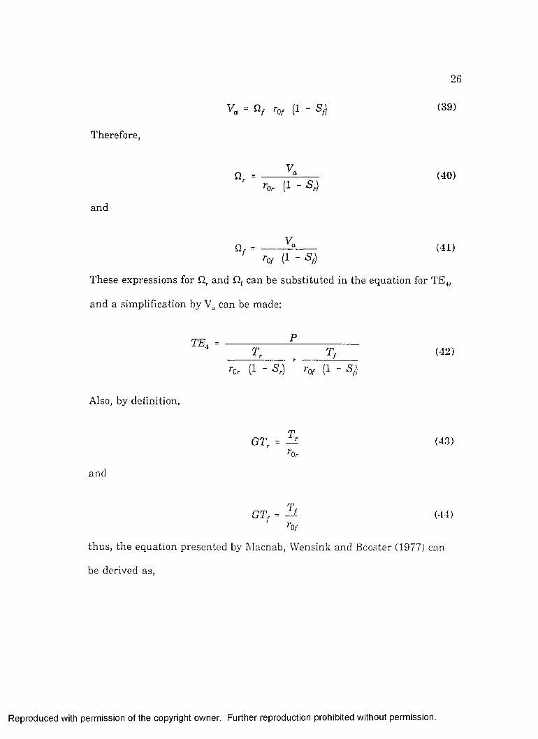
26
v ; = 0 / (1 - 6 % ( 3 9 )
Therefore,
and
Q = -------^ ------ (40)
yQ = ------- 15------ (41)
'■0/ (1 - S ,)
These expressions for Q. and flf can be substituted in the equation for TE.j,
and a simplification by can be made:
TE, =T, Tf (42)
Or (1 - *Sr) ^Qf (1 -
Also, by definition.
and
GT, = ^ (43)Or
GTf = ^ (44)To/
thus, the equation presented by Macnab, Wensink and Booster (1977) can
be derived as.
R eproduced with perm ission of the copyright owner. Further reproduction prohibited without perm ission.

2 7
TE^ =G T , G T } ( 4 5 )
Note th a t the front and rear wheel slips have been distinguished from
each other. In fact, tractor manufacturers generally give a higher
theoretical tangential velocity to the front wheels (1.0 < V^/Vj, < 1.1) on
front-wheel assist tractors to increase the power transmitted through the
front axle. The tractive efficiency for the two-wheel drive mode is a
particular case of the four-wheel drive with GTf = 0. The effect of the front-
to-rear wheel tangential velocity ratio on performance of front-wheel assist
tractors has been studied by Bashford (1985) and Bashford, Woerman, and
Shropshire (1985) under various axle weight distributions. Performance
comparisons were also made with front-wheel assist tractors operated in
2WD mode. Bashford concluded that, a t maximum tractive efficiency, a
front-wheel assist tractor operated in 4\VD mode provided a larger drawbar
pull and travelled a t higher speed than in 2WD mode. Also, Bashford,
Woerman, and Shropshire recommended a 1.01 to 1.05 front-to-rear
tangential wheel speed ratio for highest tractive efficiency.
Because power measurements at the power-take-off (PTO) are common
and easy to perform, some authors use PTO power ra ther than engine
horsepower in their calculations (Ramp and Siemens, 1990).
R eproduced witti perm ission of ttie copyrigtit owner. Furttier reproduction protiibited wittiout perm ission.

28
The term o v e ra l l e ff ic ien cy (OE) can be used to quantify the total
losses of power between the engine and the drawbar.
TJPOE = Ë (46)
HP,
F ig u r e 7 shows some typical power transmission efficiencies for tractors
having gear-type transmissions. F ig u re 8 gives an example of available
drawbar power on various surfaces for a tractor rated a t 116 hp (engine
horsepower).
For some operations, the tractor user may want to obtain the highest
net pull possible, without regard to the tractive efficiency. This is expressed
by the p u l l r a t io (o r n e t t r a c t i o n ra t io ) , which is defined as the
maximum net pull tha t can be obtained for a given dynamic load:
Generally, the highest pull is reached a t a higher slip than normal. ASAE
Standard EP 391.1 (ASAE, 1989c) gives common slip values for optimum
tractive efficiency on various soils:
Maximum TE is obtained within optimum slip ranges of:4 - 8 % for concrete8 - 10 % for firm soil11 - 13 % for tilled soil14 - 16 % for soft soil and sand.
R eproduced with perm ission of the copyright owner. Further reproduction prohibited without perm ission.

29
87-90 V. 96 -9 8 %
90-92%85-8 9 % 75-81%
94-96%
92 %86-89% * **
AXLE
DRAWBAR*
NET ENGINE
TRANSMISSION
INPUT
* M axim um for c o n c r e te t e s t tra ck a t 4 —6 p e r c e n t tra v e l r ed u ctio n D epends on so il su r fa c e v a lu es show n for c o n c r e te
(after Zoz, 1972)
F igu re 7. T ypical pow er tran sm ission e ffic ien c ies for tractors h av in g gear-type tran sm ission s
AVAILABLE HORSEPOWER (HP)
0 1 0 2 0 3 0 4 0 5 0 6 0 7 0 8 0 9 0 1 0 0 1 2 01 I I I I I ! I I ' I ! I I
PTC HP
ON CONCRETE
DRAWBAR HP ON FIRM SOIL
6 4 DRAWBAR HP ON TILLED SOB,
(a fter FARM TIRE HANDBOOK HI. Succeaaful Farm ing, A rm strong)
F igu re 8. E xam ples o f availab le draw bar pow er va lu es on various su rfaces for a tractor rated at 116 HP (engin e h orsep ow er)
R eproduced with perm ission of the copyright owner. Further reproduction prohibited without perm ission.

3 0
Maximum drawbar pull will be obtained a t higher slip values, bu t with an
increase in slip such th a t the tractive efficiency will be lower.
Consequently, tractive efficiency is the most widely accepted measure of
field performance.
O th e r P e r f o rm a n c e C r i te r ia
Persson (1991) compared the most common performance evaluation
methods and proposed the use of a coefficient called the t r a c t iv e p o w e r
ra t io , defined as:
. . • - I f
Consequently,
HP^ = W V, (-19)
According to Persson, the common method of evaluating performance at
"commonly accepted travel reduction" (between 15 and 25 %) could only be
used to compare tractive devices having a similar basic design and was
inappropriate for bias vs. radial, track vs. tire, or comparisons between
traction aids, because the selection of a fixed travel reduction value greatly
affected the results. The second method, which gave performance a t the
point of maximum tractive efficiency, was recommended when minimum
engine power, or minimum fuel consumption, were required for a certain
power output, ie. when the limiting factor was fuel consumption, or engine
power. The third method proposed by Persson evaluated performance a t
R eproduced with perm ission of the copyright owner. Further reproduction prohibited without perm ission.

3 1
maximum tractive power ratio. This value represented the maximum
tractive power th a t could be produced for a given theoretical velocity and
dynamic axle load. Persson showed tha t the maximum tractive power ratio
occured a t 50 to 70 % higher net traction than maximum tractive efficiency
(which m eant an implement 50 to 70 % larger), 20 to 40 % higher tractive
power (20 to 40 % higher capacity), 40 to 80 % higher engine power
requirements, 15 to 20 % lower actual speed for the same gear, 15 to 20 %
lower tractive efficiency, and similar fuel consumption per hectare.
Grisso et al. (1992a) proposed 3 new performance variables to better
describe the tractive performance of a tractor as a whole.
T T E a = (50)
where TTEq was the tractor tractive efficiency (dimensionless).
where DPR was the dynamic pull ratio, or vehicle traction ratio
(dimensionless). The third performance variable was used to reflect the
relative importance of tire dimensions and ballast placement.
TV N = (52)100 (IT} + TF,)
where:
TVN = tractor vehicle number (dimensionless), and
R eproduced with perm ission of the copyright owner. Further reproduction prohibited without perm ission.

32
B„f and = front and rear axle mobility numbers, respectively, as
defined later in this chapter (see Brixius traction model).
Dwyer (1984), in presenting techniques to predict tractive performance,
proposed a simple design criterion for wheeled vehicles. Knowing that
tractive efficiency generally reached a maximum for a gross-traction
coefficient of about 0.4, and tha t the highest tractive efficiency to be
a ttained in most field conditions was about 70%, Dwyer suggested the
following equation to relate axle power, weight on the driving wheels, and
vehicle travel speed:
0.7 HP^ = 0.4 IF (53)
or, by rearranging,
^ (54)W 1.75
This equation gave a quick estimate of one variable as a function of the two
others.
Because the theoretical background presented above is not easily
understandable nor usable for the tire user in general, information
brochures have been published to provide advice on selection and optimum
utilization of farm tires (The Goodyear Tire and Rubber Company, 1992 and
1994; Successful Farming, 1986 and 1988). Easy-to-use tables and graphs
were provided, along with simple methods to evaluate and increase
productivity.
R eproduced with perm ission of the copyright owner. Further reproduction prohibited without perm ission.

3 3
Tire Mechanical Properties
R o llin g R a d iu s on a R ig id S urface
Charles and Schuring Rolling Radius Model
At Firestone’s testing facility in Columbiana, Ohio, Charles and
Schuring (1984) measured the effective rolling radius of 4 types of tractor
drive tires (R-1 bias, R-1 radial, R-2 bias, and LS-2 bias forestry tires) as a
function of tractor speed, tire load, tire pressure, and state of hydroinflation.
They used statistical analysis to develop an empirical model. Five tractor
speeds between 0.8 km/h and 28.8 km/h, 3 inflation pressures (83 kPa, 110
kPa -ie. rated, and 138 kPa), 3 loads (rated minus 25%, rated, rated plus
25%), and 3 states of hydroinflation (0%, 75%, and 90%) were considered.
Three replications of each measurement were used for each of the 4
different types of tires. Ten variables were considered to possibly affect the
effective rolling radius; 1) load on axle, 2) tire inflation, 3) degree of
hydroinflation, 4) tire t>pie and size, 5) ply rating, 6) consti-uction (radial or
bias), 7) tread design, 8) position on tractor (front or rear), 9) tractor model,
and 10) tractor speed. All tests were conducted a t zero drawbar pull. The
equation for this model was:
rjj = ( l - h ) r ^ + k (55)
where the unloaded stationary tire radius r^ was measured as the tire
circumference (C) measured over the lugs, in the center plane of the tire.
R eproduced with perm ission of the copyright owner. Further reproduction prohibited without perm ission.

3 4
and divided by 2k. The effective rolling radius r^ was computed as,
= (56)2 K N Q
where;
X = distance traveled by tire, and
N = num ber of revolutions required by tire to traverse distance X.
Rearranging the model equation:
- ^R (57)
Note th a t r,; could theoretically vary between 0 (spinning tire) and infinite
values (locked tire), bu t it was generally between r, and r^:
(58)
This m eant th a t k remained between 0 and 1. Typical values of k
determined by Charles and Schuring are given in T ab le 1. F ig u re 9 below
shows the difference between r^, r^ and r^.
T a b le 1. V a lu es o f k fo r F o u r T r a c to r T ires , M e a s u re d a t Zero D r a w b a r P u l l (C h ar le s a n d S c h u r in g , 1984)
T i re te s t e d T r e a d d e p th k v a lu eR-1 bias (general purpose) 40.9 mm 0.63
R-2 bias (deep lug) 81.0 mm 0.74LS-2 bias (forestry) 51.1 mm 0.56
R-1 radial (general purpose) 40.9 mm 0.40
R eproduced with perm ission of the copyright owner. Further reproduction prohibited without perm ission.

3 5
F igu re 9. D ifferen t w h eel radii u sed by C harles and S ch u rin g (1984).
Most of the test variables had no influence on k because their effects were
already reflected by the static loaded tire radius r^. Only carcass
construction and tread depth appeared significant. Construction was the
most significant. Radial tires showed a distinctly lower value of k, meaning
th a t was closer to ly. for radiais than for bias-ply tires. Charles and
Schuring attributed this to the nearly inextensible belt which maintained
the rolling circumference of the radial tires close to the unloaded
circumference. Without this belt, r^ for bias-ply tires tended more towards
their loaded circumference divided by 2k. The k values increased wdth tread
depth for all tires. The average coefficient of variation (C.V.) of the k values
was ra ther low (about 10%).
R eproduced with perm ission of the copyright owner. Further reproduction prohibited without perm ission.

36
C la rk R o ll in g R a d iu s M odel
Clark (1981) described a similar model for use with truck and passenger
car tires. The model proposed by Charles and Schuring may be considered
as a particular application of a more general model.
B r ix iu s a n d W ism er R o llin g R a d iu s M odel
Earlier work by Brixius and Wismer (1978) showed that:
0.85 < - ^ < 0.95 (59)
Which implied,
0.61 < k < 0.64 (60)
Also,
rR2.5 r^j _ 2.5 r^
(61)
Substituting into the equation by Charles and Schuring for k, and
simplifying.
k = - 1 - 5
R eproduced with perm ission of the copyright owner. Further reproduction prohibited without perm ission.

3 7
S ta tic D eflec tio n , S tiffn ess and C ontact A rea on R ig id S u rface
Several characteristics were listed by Abeels (1976) to describe the
behavior of tires under static loads:
- T ire d eflection , or tire sec tio n h e ig h t vs. load curve;
- O verall tire sec tio n w id th vs. load curve;
- L evel h^, at w h ich th e sec tio n w id th is m axim um , vs. load curve;
- Ratio between tire section height and overall section width (hyb„) vs. load
curve;
- S q u ash ra te t vs. load curve. The squash rate, or budding ra te of the
sidewalls is defined as,
^ * 100%] (63)h
where:
h = unloaded tire section height (m), and
h , - loaded tire section height (in).
- F l a t t e n in g r a t e t^ vs. load curve. The flattening rate is defined as,
f = & ...r 9 * 100%) (64)K
where:
b„ = overall unloaded tire section width (m), and
b„ = overall loaded tire section width (m).
R eproduced with perm ission of the copyright owner. Further reproduction prohibited without perm ission.
38
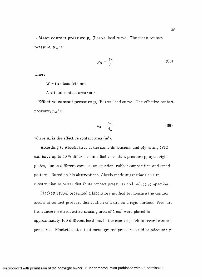
- M ean co n ta ct p ressu re (Pa) vs. load curve. The mean contact
pressure, p„,, is:
^ (65)A
where:
W = tire load (N), and
A = total contact area (m").
- E ffective co n ta ct p ressu re p (Pa) vs. load curve. The effective contact
pressure, p ,, is:
WPa = ^ (66)
" a
where is the effective contact area (m“).
According to Abeels, tires of the same dimensions and ply-rating (PR)
can have up to 40 % difference in effective contact pressure p upon rigid
plates, due to different carcass construction, rubber composition and tread
pattern. Based on his observations, Abeels made suggestions on tire
construction to better distribute contact pressures and reduce compaction.
Plackett (1984) presented a laboratory method to measure the contact
area and contact pressure distribution of a tire on a rigid surface. Pressure
transducers with an active sensing area of 1 cm' were placed in
approximately 100 different locations in the contact patch to record contact
pressures. Plackett stated tha t mean ground pressure could be adequately
R eproduced with perm ission of the copyright owner. Further reproduction prohibited without perm ission.

3 9
defined as the sum of inflation pressure and carcass pressure (pressure due
to the tire carcass stiffness). Once contact area was known for a given
inflation pressure, carcass pressure could be determined. Tire stiffness was
computed for various inflation pressures as the slope of the load vs.
deflection curve. Carcass stiffness was then found by extrapolation, as the
tire stiffness a t zero inflation pressure. Plackett also reported tha t radial-
ply tires provided a more even distribution of ground pressure, with peak
values approximately 15% smaller than those for bias-ply tires under the
same conditions. Peak values exceeded the measured mean ground
pressures by a factor of 2 to 2.6, depending upon inflation pressure, load
and carcass construction.
Upadhyaya and Wulfsohn (1990a) presented equations tha t can be used
to relate the size of the contact area to the deflection of tires. The contact
area is an important factor in traction because it has a direct effect on
contact pressure and gross pull. A simple method of measuring contact area
was used. For a given inflation pressure, the tire was pressed with the
desired vertical load against a steel plate covered with a white sheet of
paper, and a carbon paper. The tire was then raised, rotated by a few
degrees, and loaded again. This operation was repeated four to five times to
obtain a neat imprint of the contact area. The length, the width, and the
area of the contact patch were measured directly on the imprint. Tests
were conducted for 3 tire sizes: 16.9R38, 18.4R38, and 24.5R32. Loads of
R eproduced with perm ission of the copyright owner. Further reproduction prohibited without perm ission.

4 0
17.8 kN, 22.2 kN, and 26.7 kN were applied to each tire. Inflation
pressures of 83 kPa, 103.5 kPa, and 124 kPa were applied to the 18.4R38
tire. The 16.9R38 and 24.5R32 tires were both tested under inflation
pressures of 83 kPa and 124 kPa. A geometrical analysis lead to the
following equations, wliich were validated through linear regression analysis
of the test data.
Z = 2 \[E~d ( 6 7 )
L = S # ”ô " " i / L <
“ ^tread Otherwise(68)
A = (tt - 2 q) ( 6 9 )
where:
and,
0 otherwise
\ u; / \{ h \Cread
tread (70)
A = contact area (mh,
1„ = contact width (m),
1 - contact length (m),
Krcud = tread width (m),
R., = unloaded, outside radius of the tread in a plane transverse to the
R eproduced with perm ission of the copyright owner. Further reproduction prohibited without perm ission.

4 1
tire (m), and
^ = empirical correction factor equal to 0.782 for Upadhyaya's data,
and equal to 0.629 for a given tire m anufacturer’s data.
The dimensions used by Upadhyaya and Wulfsohn are shown in F ig u r e 10.
tread
F ig u r e 10. T i re d im e n s io n s u s e d b y U p a d h y a y a a n d W ulfsohn (1990) in t i r e d e f lec t io n a n d c o n ta c t a r e a m ode l
Pain ter (1981) developed an empirical equation relating load to
deflection and inflation pressure:
a, / . / - \-0i0
Co
bj( 7 1 )
where:
a, and a = constants greater than 2,
R eproduced with perm ission of the copyright owner. Further reproduction prohibited without perm ission.

4 2
ao and a^ = constants less than 0.5 (by amounts which depend on the
ranges of values of S/d and 5/b,),
Eiq = constant introduced to allow for an intercept in empirical fitting
(equivalent to a value of load which produces no measurable
deflection a t zero inflation pressure),
aj = constant tha t would represent tire elastic stiffness i f there was
no other term on the right side of this equation,
dj, = tire diameter at root of tread on centerline (m, usually
approximated to be the tire overall diameter d since tread height is
small compared to d ), and
bg = tire cross section equivalent diameter of curvature (m).
Coefficients a , a,, a. , a , a and a were found by empirically fitting curves
to test data. The theoretical relationship used to deidve the above equation
can be developed as follows:
p ' y l = + . E , 0 = ( 7 2 )
where:
A, = equivalent contact area (nr),
A = contact area (m').
Kg = tire carcass stiffness (N/m), and
p' = mean value of contact normal stress (Pa).
The terms A„p and are the pneumatic and the elastic terms,
respectively. The following h}-potheses were used:
R eproduced with perm ission of the copyright owner. Further reproduction prohibited without perm ission.

4 3
1. Ag = elliptical contact area which the carcass alone would make on a
smooth, rigid surface when deflected by 5;
2. The equivalent diameter of curvature of the cross-section (bg) can be
defined.
In general, for front tires.
- 5- < 0.1 (73)
and for rear tires.
< 0.05 (74)
also, for all tires.
— < 0.2
For small ratios 6/dy and 6/b (small deflections).
IF •f --:2 T . X 4
-1
cos' 1 -26 cos' 26
(75)
( 7 6 )
where the term (K/p6) is the elastic term, and the remainder of the
expression is the pneumatic term.
Blaszkiewicz (1990) adopted a similar approach as tha t used by
Upadhyaya and Wulfsohn (1990a), and Painter (1981). A tire theoretical
model was developed through geometrical analysis before being matched to
experimental data. Komandi (1976) proposed a completely empirical model
R eproduced with perm ission of the copyright owner. Further reproduction prohibited without perm ission.
4 4
by fitting equations to experimental data without any preliminary
theoretical consideration on the forms of tire characteristic equations. This
type of model, though adequate for simulation purposes, did not yield any
explanation of the mechanical behavior of tires.
D y n a m i c S t i f f n e s s a n d D a m p i n g S t u d i e s
Most of the published research dealing with tire stiffness and damping
coefficient was aimed a t the dynamic behavior of agricultural vehicles to
protect operators from overturns, shock and ribration, and to increase
comfort. The studies either considered the tires separately and then
included them in a more general vehicle dynamic model, or a complete
vehicle was studied a t once. For example, Freeland et al. (1990) studied
chassis accelerations on a lawn and garden tractor on which three strain
gauge accelerometers were installed to measure vehicle shock response
following rea r tire impact. Shocks were initiated by letting the rear axle of
the tractor fall from a 0.18 m height for the non-rolling case, and by letting
a pole fall in front of the rear axle, between the two axles, for the rolling
case. Data acquisition procedure, waveform analysis, and reporting
procedures were developed tha t closely conformed to SAE and ISO
recommendations for measuring operator seat vibrations of off-road vehicles.
Laib (1979) measured the static stiffness in the vertical direction for
tractor tires a t various inflation pressures. At first, stiffness increased with
load, then remained constant, or even decreased slightly. Stiffness also
R eproduced with perm ission of the copyright owner. Further reproduction prohibited without perm ission.

4 5
increased with inflation pressure. Rolling tire stiffness measurements
showed th a t travel speed had little effect on stiffness between 3 and 5 m/s
(11 to 18 km/h). However, stiffness first decreased (10 to 20 % for bias-ply
tires) a t increasing rolling speed, then started increasing again with speed,
for radial as well as for bias-ply tires. The damping coefficient decreased
when rolling speed increased, when inflation pressure decreased, and also
when the frequency of vertical excitation increased. Laib proposed an
empirical equation relating the damping coefficient to the excitation
frequency:
Cj = (77)
where:
Cj = damping coefficient (s N/m),
f = excitation frequency (Hz), and
ki and k^ = empirical coefficients.
Janssen and Schuring (1985) presented several equations for the
deflection versus load curves of agircultural tires in various directions. The
equation describing the relationship between the vertical load and the
deflection was of the form,
IF = Ô + Co ô'' (78)
where c,, c., and Cg were empirical coefficients.
R eproduced with perm ission of the copyright owner. Further reproduction prohibited without perm ission.

4 6
Dimensional and regression analyses of static deflection-versus-load curves
for 15 bias-ply and 7 radial-ply tires a t various inflation pressures were
used to determine coefficients Cj, c , and C3, which are functions of tire
construction, inflation pressure, dimensions, and load capacity. Tire section
vndth ranged from 13.6 to 30.5 inches and rim diameter ranged from 26 to
42 inches. The following equation was developped:
W - E q à + Kq/ , \ 1.6
0
V ^ rated I
(79)
where:
I\) = initial stiffness (N/m), or stiffness a t origin (zero load, zero
deflection),
Wratc-d = design load a t given inflation pressure (N), and
5ratcd = deflection a t design load (m).
This equation was simplified to,
= jroô + 6%?(ioo ay s (so)
where SF was a coefficient called s t i f fe n in g fac to r . Also,
= I - p) (81)
and,
Zq = -3.25 + 0.12 h + 0.39 C O N ST - 0.47 R IM + 6 p (82)
R eproduced with perm ission of the copyright owner. Further reproduction prohibited without perm ission.

4 7
where:
@ p) = static loaded tire radius for the ra ted load a t
inflation pressure p,
CONST = constant defining tire construction (2 for bias tires,
and 3 for radial tires), and
RIM = constant associated with rim diameter (1 for diameters
less than 30 inches, 2 for diameters 30 inches or greater).
Dynamic characteristics (stiffness and damping coefficient) were determined
by imposing a sinusoidal forcing function on the axle of the deflected tire
and measuring the system response as a function of the forcing frequency in
rolling condition. The amplitude of the forcing function was not given. A
forcing frequency well below the resonant frequency of the tire was used to
determine stiffness, and the response a t resonant frequency permitted the
calculation of the damping coefficient. T ab le 2 gives the characteristics of
the tires tested and the results obtained.
Collins (1991) pointed out the importance of tire dvmamic properties to
predict the dynamic beha\’ior of tractor-implement systems during road
transport. A ride simulation model based on Lagrange’s equation was
proposed. This model was specifically designed to predict dynamic loads in
tractor three-point hitches and it was validated by comparing predicted
hitch load values with the dynamic measurements on an agricultural tractor
carrying an implement mounted on its three-point hitch. Each tire was
R eproduced with perm ission of the copyright owner. Further reproduction prohibited without perm ission.

48
T able 2. S tiffn ess and D am ping C haracteristics o f T ires as M easured b y J a n ssen and S ch u rin g (1985)
Tire In fla tion pressure (kPa)
110 138 165 220
18.4R38 (kN) 23.36 26.61 29.64
5rated (™) 0.085 0.085 0.085Ko (kN/m) 169 187 203SF 0.293 0.350 0.404
@ 80% 6 (kN/m) 270 307 342(kN/m) 344
Cj (skN/m) 2.818.4-38 (kN) 23.36 26.61 29.64
Srated (m) 0.081 0.081 0.081Kg (kN/m) 130 148 164SF 0.448 0.511 0.571
@ 80% 6 (kN/m) 301 334 370(kN/m) 364
Cj (skN/m) 3.014.9R26 W,„ted (kN) 13.43 15.30 17.26 2&2
Grated (m) 0.059 0.059 0.059 0.059Kg (kN/m) 804) 97.6 113JS I j #SF 0.509 0.553 0.611 0.680
@ 80% 6 (kN/m) 231 262 296 347IVoiiin« (kN/m) 385Cj (skN/m) 2.1
14.9-26 Wr., .j (kN) 13.43 15.30 17.26 2 0 ?Grated (^) 0.058 0.058 &058 0.058Kg (kN/m) 41 59 75 108SF 0.655 0.699 0N60 0.940
@ 80% 6 (kN/m) 235 266 300 386Krallinx (kN/m) 417Cj (skN/m) 2.2
assumed equivalent to a spring and a damper in parallel for its d^mamic
behavior in the vertical direction. Non-rolling values of stiffness and
R eproduced with perm ission of the copyright owner. Further reproduction prohibited without perm ission.

4 9
damping coefficient were used because they were of the same magnitude as
rolling values, although previous research by other investigators had shown
tha t rolling tire properties were significantly different from non-rolling
properties. However, simulation results compared satisfactorily to
experimental measurements of the vertical and pitch accelerations for the 0
to 6 Hz excitation frequency range. Thus, stiffness and damping coefficient
of non-rolling tires may be considered satisfactory for simulation purposes.
The characteristics of the tires used in tha t experiment are given below:
Front unloaded tire radius = 0.43 m
Front rim radius = 0.25 m (20-inch diameter rim)
Vertical front tire stiffness = 550 kN/m
Vertical front tire damping coefficient = 2.350 s-kN/m
Rear unloaded tire radius = 0.77 m
Rear rim radius = 0.51 m (40-inch diameter rim)
Vertical rear tire stiffness = 600 IcN/m
Vertical rear tire damping coefficient = 5 shN /m
Lines and Murphy (1991) measured the dynamic stiffness of rolling
agricultural tires in the vertical (radial) direction. Environmental variables
were: tire inflation pressure, rolling speed, tire load and deflection,
amplitude of vibration, frequency of vibration, and surface type. Tire
dependent variables were: tire size, tire construction, ply rating, lug length,
age, wear and rubber composition. The experimental machine used in this
R eproduced with perm ission of the copyright owner. Further reproduction prohibited without perm ission.

5 0
research project was described earlier by Lines and Young (1989). Tires
were mounted on a carriage behind a tractor. An electro-hydraulic actuator
was used to vibrate the carriage against an inertial mass. The recorded
signals were the force on the test tire and the acceleration of the carriage
axle. The stiffness and damping coefficients were derived from the
differences in magnitude and phase of the two signals. M easurements were
made both stationary, and rolling at speeds of 0.1 to 25 km/h. Various
surfaces were used to study their effect. Linear regression analysis was
used to identify the most significant variables and lead to the following
equation:
K = 112 - 1.77 + 5.6 o + 0.34 h p (S3)
where the inflation pressure, p, was expressed in bars, and:
K = tire stiffness (kN/m),
d,-im = rim diameter (in.),
b = tire section width (in.), and
a = tire age (years).
Although prior research showed tha t tire stiffness and damping coefficient
changed with rolling speed. Lines and Murphy found tha t rolling speed was
significant only below 15 km/h. Load, torque, construction and ply rating
were found to have no significant influence on stiffness. Other variables
only had a small influence. Lines and Mui-phy also found a linear
relationship between stiffness and inflation pressure:
R eproduced with perm ission of the copyright owner. Further reproduction prohibited without perm ission.

5 1
K = K , * p AEp (84)
where:
Kg = carcass stiffness (kN/m), and
AKp = inflation pressure dependence (kN/m.bar).
This equation becomes similar to the load equation proposed above by
Pa in te r when multiplied by the deflection on both sides, thus showing
agreem ent between researchers. Also, by assuming that, for the range of
normal tire deflection, the width of the contact area remains constant and is
proportional to the tire section width, and by assuming th a t the effective
contact-patch length is proportional to the tire deflection and the tire size as
given by the rim diameter:
= O.EWb (85)
Spring-and-damper models have been used for numerous tire and
vehicle behavior simulation purposes. Thompson, Liljedahl, and Quinn
(1972) proposed a model where a spring and a damper were in parallel to
represent the motion of a tire running over obstacles. Baladi, Rohani, and
Barnes (1984) developed a model with a set of radial composite springs both
for a tire and the soil under it. Each composite spring consisted of two
springs in series, one for a portion of the tire and the other for the
corresponding soil section. The stiffness of the springs depicting the soil
was derived from the theory of soil ca\dty expansion.
R eproduced with perm ission of the copyright owner. Further reproduction prohibited without perm ission.

5 2
Ruminer (1989) used a stiffness of 763700 N/m and a damping
coefficient of 4800 sN/m in a parallel spring-and-damper tire model for
computer simulations of ride dynamics of a log-skidder equipped with four
67/34.00-25 tires inflated at 172 kPa. The values of stiffness (or spring
rate) and damping coefficient had been obtained through measurements on
actual machines, bu t no detail was given about the way these values had
been measured.
Crolla, Horton, and Stayner (1990) also used a parallel spring and
damper system to simulate tire mechanical properties in the vertical
direction, although they recommended the use of another type of system
(spring and damper in series) for the lateral and longitudinal directions.
Ten different tractors were used to compare measured data to predictions
obtained through a simulation program called VDAS (Vehicle Dynamics
Analysis Software) tha t had been developed at the University of Leeds, UK.
The tractors were run a t various speeds on a special track and accelerations
in the 3 directions (longitudinal, lateral and vertical) were measured under
the driver seat. Although tire sizes were not indicated by Crolla, Horton,
and Stayner, tire stiffness and damping coefficient values were given as
reported in T ab le 3 as sample values. These values were measured with
non-rolling tires on a static test stand providing step inputs in each
direction (vertical, longitudinal, and lateral).
R eproduced with perm ission of the copyright owner. Further reproduction prohibited without perm ission.

5 3
Table 3. S tiffn esses and D am ping C oefficients U sed by Crolla, H orton, and S tayn er (1990)
T ractor type Front tire vertica l stiffn ess (kN/m)
Front tirevertica ldam pingcoeffic ien t(skN/m)
R ear tire vertica l stiffn ess (kN/m)
R ear tirev ertica ldam pingco effic ien t(skN/m)
2\VD 330 4.500 400 5.0002WD 332 4.164 340 3.3112WD 377 4.230 360 &188
4\VD with unequal sized wheels
332 3.418 432 3T94
4\VD with unequal sized wheels
571 4.542 465 4.388
4WD with equal sized wheels
653 &002 564 5.269
4\VD with front suspension
460 2.250 460 2.250
4\VD with front and rear suspension
642 4.462 642 4.462
2\VD 377 4.230 360 2.1882\VD with front
suspension377 4.230 360 2.188
Rising and Gohlich (1989) measured dynamic characteristics of some
agricultural tires, both under rolling and non-rolling conditions. They
concluded tha t these tires had nonlinear stiffness characteristics, especially
under non-rolling conditions. In all cases, stiffness increased with deflection
and with inflation pressure. Stiffness values were also observed to be about
25 % greater for non-rolling tires than for rolling ones. Also, the damping
coefficient decreased substantially with increasing speed, decreased slightly
R eproduced with perm ission of the copyright owner. Further reproduction prohibited without perm ission.

5 4
with inflation pressure, and remained practically constant for traveling
speeds above 30 km/h.
Siefkes and Gohlich (199?) studied the dynamic behavior of low-
pressure, wide-section agricultural tires and compared them with more
common tires of similar overall diameter. The study focused on vibrations
due to tire circumferential nonuniformities (also called tire runout) and to
lugs, especially a t high linear speeds up to 40 km/h. Vertical stiffness and
damping coefficient were determined through a method using natural
frequency and logarithmic decrement. The tires were mounted on the
special outdoor tra iler of the Berlin Institute of Agricultural Engineering,
which was pulled a t various speeds ranging from 0 to 40 km/h, on a paved
road. No torque was applied to the tires, and slip was therefore considered
to be zero (free-rolling wheel on hard surface). Linear velocity and vertical
forces on the axle were recorded. Vertical stiffness decreased by 207c to
25% of its static value when speed increased from 0 to 10 km/h, and
remained almost constant from 10 km/h to 60 km/h. It increased with
inflation pressure and load. Bias-ply tires were 10 to 207c stiffer than
radiais of similar sizes. The vertical damping coefficient increased when
speed increased from 0 to 5 km/h, and decreased when speed increased from
5 to 50 km/h, where it reached a limit value approximately equal to 30% of
its value a t 0 km/h. It increased with load, and decreased when inflation
pressure increased. Bias-ply tires had a higher damping coefficient than
R eproduced with perm ission of the copyright owner. Further reproduction prohibited without perm ission.

5 5
radiais a t low inflation pressure, but the difference was not measurable at
higher inflation pressures.
Barrelmeyer et al. (1993) proposed a nonlinear model for tire vertical
behavior. The model used a spring and a damper in parallel to represent
the tire, but the stiffness of the spring increased with deflection, and the
damping coefficient decreased with rolling speed. The model was fitted to
limited experimental data and further experiments were required for
validation.
Both stiffiiess and damping coefficient proved necessary in the
development of mathematical models to be used in dynamic simulations and
in the description of tire mechanical characteristics. However, most models
described only one of the two variables, K or Cj, and the influence of
inflation pressure and excitation frequency needed to be more completely
assessed. Therefore, the development of a machine to measure both
characteristics simultaneously appeared necessary.
E f f e c t o f I n f l a t i o n P r e s s u r e
Czako (1974) studied the influence of tire inflation pressure on the
mobility of two 6x6 military trucks, each equipped with a central tire
inflation/deflation system. According to Czako, such systems have been well
known since World War II for increasing vehicle mobility on soft soil by
decreasing inflation pressure in soft soil conditions. On wet loam, the
maximum drawbar-pull increased by 19% for one truck, and by 20% for the
R eproduced with perm ission of the copyright owner. Further reproduction prohibited without perm ission.

5 6
other when inflation pressure was reduced from 241 to 103 kPa. When
inflation pressure was further decreased to 48 kPa on one of the trucks, the
maximum drawbar pull increased 39%. On fine sand, the increases in
maximum drawbar-pull reached 22% and 26% for each truck, respectively,
as inflation pressure dropped from 241 to 103 kPa. On coarse sand, drastic
increases in maximum drawbar-pull were observed with values of 90 and
66% for the same pressure drop. On dry loam (hard soil), however, the
increases in maximum drawbar-pull were less significant, with values of 4%
and 8%.
B urt and Bailey (1982) investigated the effects of load and inflation
pressure on a 20.8R38 8-ply rating tire. Two t}-pes of tests were conducted.
In the first type, dynamic load was continually and slowly increased from
zero to a value causing excessive tire deflection, while both travel reduction
and inflation pressure were maintained constant. In the second tests, travel
reduction was maintained either a t 10 or 20% and dynamic load was held
constant a t either 60 or 100% of the Tire and Rim Association rated static
load a t maximum pressure, wliile inflation pressure increased from a value
causing a large tire deflection to the maximum value. For travel reduction
calculations, the tire rolling radius was determined experimentally as a
function of d}mamic load and inflation pressure, on concrete, at zero net
traction. Burt and Bailey concluded that, by selecting appropriate levels of
dynamic load and inflation pressure, tractive efficiency could be improved
R eproduced with perm ission of the copyright owner. Further reproduction prohibited without perm ission.

5 7
by 6 to 10%, depending on the soil conditions. In general, tractive efficiency
and net traction increased while inflation pressure decreased. The dynamic
loads encountered a t maximum tractive efficiency were not unusually high
in comparison with typical field conditions and did not seem to compromise
tire durability under reduced inflation pressure.
Wood and Mangione (1992) conducted a field demonstration, where two
identical tractor-implement combinations operated in similar field
conditions but with different tire inflation pressures. Both tractors were
276 kW (370 hp) four wheel drive John Deere 8960’s equipped with dual
20.8R42 radial-ply tires and the implements were DMI Tiger-Two 7-shank
subsoilers. On one tractor, tire inflation pressure was set a t 165 kPa for
the inner duals and 152 kPa for the outer duals, according to common
practice among the farmers of the surrounding area. The other tractor had
97 kPa and 83 kPa inflation pressures for its inner and outer duals,
respectively, according to Tire and Rim Association recommendations for the
actual load per tire. The tractor with the lowest inflation pressure showed
significant slip reduction and increase in field productivity, but the effect of
tire brand was ignored (one tractor had Ajrmstrong tires while the other had
Goodyear tires).
Erbach and Ivnoll (1992) studied the effects of load and tire inflation
pressure on soil compaction, evaluated by bulk density, cone index, and
hydraulic conductivity measurements. Three rear axle loads (24, 37 and 49
R eproduced with perm ission of the copyright owner. Further reproduction prohibited without perm ission.

5 8
kN) and two inflation pressures (80 and 200 kPa) were used on a White 160
wheeled tractor. Two track loads (37 and 49 kN) producing nominal soil
surface contact pressures of 32 and 43 kPa were also applied through a
D3BSA Caterpillar tracked tractor. Erbach and Knoll concluded tha t soil
bulk density increased with contact pressure, which increased with load and
inflation pressure. Hydraulic conductivity and cone index measurements
showed a high degree of variability and no correlation with contact pressure
could be established. Also, the effect of increasing contact pressure tended
to increase with load.
Bashford, Al-Hamed, and Jenane (1992) compared the tractive
performance of 3 types of tires (18.4R42, 18.4R46 and 12.4R54) when
mounted on the rear axle of a front wheel assist tractor. Front tires were
matched to the rea r tires with respect to tangential velocity. The front tires
were of the 14.9R28 type for the rear 18.4R42, 16.9R30 for the 18.4R46, and
16.9R30 for the 12.4R54, respectively. Two types of soil, described as soft
and firm, and 3 levels of inflation pressure (55, 83 and 124 kPa) were used
during the experiments. All rear tires were mounted as duals and only the
124 kPa inflation pressure was used for the 12.4R54 tires because of their
lower load carrying capacity. In general, tractive efficiency increased with
rim diameter and with decreased inflation pressure. Bashford et al. used
the Gauss-Newton method of non-linear regression to fit the Wismer-Luth
traction equations to their data.
R eproduced with perm ission of the copyright owner. Further reproduction prohibited without perm ission.
5 9
According to Collot (1988), Massey-Ferguson engineers have developped
a central tire inflation system for a MF 3090 tractor. Inflation pressure in
the rea r wheels can be adjusted a t will by an engine-mounted air
compressor, two air tanks located under the cab, ro tating seals on the rear
axle, and two valves mounted in the rims. The system is monitored from
the cab. The main advantages of this system are:
- lower soil compaction, due to reduced tire-soil interface pressure and
increased contact area,
- reduced slip on wet soil,
- reduced slip variations,
- longer tire life due to optimization of tire inflation pressure, and
- greater comfort for the di'iver on the highway.
Collot mentioned th a t dynamic load was not used directly for the
determination of the optimum inflation pressure. The ability to estimate
this factor appeared to be left to the judgment of the driver. However, an
iteration process may help the driver approach optimum inflation pressures
through trial and error, where travel speed and engine speed may be the
variables used by the driver. The advent of velocity radar systems, on
board electronic monitoring devices, and driving aids on European tractors
indicated opportunities for further improvement in this system.
R eproduced with perm ission of the copyright owner. Further reproduction prohibited without perm ission.

6 0
Traction and Power Measurements
Traction and power measurements have been made on numerous
occasions and for various purposes, the most significant being to compare
tractive devices for performance, to study the effect of different variables
(tire dimensions, inflation pressure, load, carcass construction ...etc), and to
predict tractive performance. For example, B urt and Lyne (1985) studied
the effect of travel velocity on net traction and tractive efficiency of an 18.4-
34 and an 18.4R34 tires in soil bins. They found no significant effect of
travel velocity within the 0.36-2.16 km/h speed range. But travel velocities
ranging from 2 to 7 km/h were used by Greenlee, Summers, and Self (1986)
to study the effect of travel velocity on net traction in the field with five R-1
tires (8.3-24; 11.2-38; 15.5-38; 16.9-30; 18.4R38) propelled by the
Oklahoma State University single wheel tester described by Self et al.
(1986). The travel velocities tested had a significant effect on net traction.
An equation, obtained through dimensional analysis and nonlinear
regression with the NLIN procedure of the SAS software, was proposed to
include the effect of travel velocity in traction models. Other
measurements, for example, aimed at predicting tractive performance of
tractors equipped with dual tires (Wang and Domier, 1989), or comparing
the behavior of very wide tires with th a t of dual tires (Dwyer and Heigho,
1984k
R eproduced with perm ission of the copyright owner. Further reproduction prohibited without perm ission.

6 1
E x p er im en ta l P roced u res
Brixius and Wismer (1978) studied the effects of wheel slip on traction
and tractive performance. They differentiated several zero conditions for
the measurement of slip and they explained how these conditions affected
the results. Four different zero conditions were listed:
- zero torque (towed condition) on a hard surface;
- zero torque (towed condition) on a test surface;
- zero pull (self-propelled condition) on a hard surface;
- zero pull (self-propelled condition) on a test surface.
The zero pull, hard surface condition was independent of surface properties,
and thus provided a single m easurement of effective rolling radius to be
used in torque, force and slip calculations. Therefore, it was recommended
for all slip measurements, because it provided a constant numerical base for
evaluating the relative motion between the tires and the supporting surface.
I t was also the easiest condition to achieve practically. The "zero pull on
test surface" condition corresponded to the definition of travel reduction.
which depended on the test surface (soil strength), and thus did not have a
fixed base tha t could be used over a wide range of test conditions. Brixius
and Wismer did not find any statistically significant numerical difference
between the zero torque and zero pull on hard surfaces. They discussed the
effects of differences between the rolling radius measured on hard ground
and the actual rolling radius (or effective moment arm) in the soil, on the
R eproduced with perm ission of the copyright owner. Further reproduction prohibited without perm ission.

6 2
estimate of torque, gross pull, and motion resistance. They mentioned tha t
tractive efficiency usually peaked between 10-15% slip, with a pull/weight
ratio of 0.25 to 0.36 in wet conditions for 18.4-38 and 18.4R38 tires. This
was in partial agreement with the slip values given in ASAE Standard
EP391.1 (ASAE, 1989c). Using the earlier traction model of Wismer and
Luth (1973) with an additional equation to estimate the rolling radius (see
rolling radius models), Brixius and Wismer introduced the concept of the
design tractive efficiencv curve, a compromise between pull/weight ratio and
tractive efficiency over the slip range, as a guideline for designers.
Murphy and Green (1969) discussed the traction techniques used in a
soil bin a t the U.S. Waterways Experiment Station (USWES), Vicksburg,
Mississippi. The drive mechanism of the single-wheel tester used by this
research center made two types of traction tests possible: controlled slip and
controlled pull. In the controlled-slip technique, the test wheel was driven
a t a constant angular velocity under a given load, and the wheel carriage
travelled either a t constant speed (constant-slip test) or a t a uniformly
varying speed (programmed-slip test). In the controlled-pull technique, the
test wheel was didven a t a constant angular velocity, the carriage drive was
disengaged, and an external draft load was applied to the carriage to set the
net pull. Tests were performed with two different pneumatic tires on Yuma
sand from the Arizona desert. The controlled-slip technique proved more
R eproduced with perm ission of the copyright owner. Further reproduction prohibited without perm ission.

6 3
reliable than the controlled-pull method for both pull-slip and torque-slip
measurements.
Upadhyaya et al. (1988) also studied the effect of testing method on
traction test results for an 18.4R38 tire inflated a t 124 kPa, with an
approximate load of 24 kN. Tests were conducted both in a firm and a
tilled Yolo-loam soil. Constant-slip, varying-slip, constant net pull and
varying net pull tests were made. In the varying-slip tests, slip increased
from zero to a value judged as excessive, then was reduced gradually to
zero. In the varying net-pull tests, draft load increased from zero to a value
producing excessive slip, then was reduced gradually to zero. The constant-
slip technique produced the most consistent and repeatable results. Most of
the scatter in da ta appeared for low slip values and in the soft soil. The
methods ranked as follows, in order of decreasing consistency in the results
(increased scatter in the data):
- constant slip,
- constant draft,
- variable draft, and
- variable slip.
Upadhyaya et al. then discussed the effect of zero slip condition selection on
motion resistance calculations. They recommended the "zero net traction on
the test surface" as the zero slip condition, although this method was
heavily criticized by another scientist (Freitag, 1990). Upadhyaya (1990)
R eproduced with perm ission of the copyright owner. Further reproduction prohibited without perm ission.

6 4
justified this choice by the high accuracy obtained by his data regression
technique when using this method.
Upadhyaya, Sime, and Rubinstein (1992) also discussed various types of
statistical designs for tire testing experiments in order to optimize the
amount of information obtained from test results. A technique called the
i n d ic a to r v a r ia b le t e c h n iq u e was recommended and its implementation
presented in a typical example.
T e s t T r a c k M e a s u r e m e n t s
For m any years, measurements of tractor tractive performance were
carried on paved tracks to enable tractor makers to test their new designs,
tire manufacturers to test their tires, and users to compare various tractors
of similar sizes. Tests were carried out by tire and tractor manufacturers,
research scientists, and official testing centers, such as the Nebraska Test
Laboratory, and test centers affiliated with the Organization for Economic
Cooperation and Development (OECD). During the tests, tractors were run
on paved surfaces (concrete, or other), a t different speeds and with various
drawbar loads. The drawbar loads were usually provided by a load vehicle,
like tha t described by Nation and Jesson (1957), which basically
transformed drawbar power into dissipated heat through an electrical,
hydraulic, or mechanical circuit. Nebraska Test Reports, done a t the
University of Nebraska, Lincoln, Nebraska, were published for all tractors
sold in the U.S. market. Buckingham (1985a and 1985b) described the
R eproduced with perm ission of the copyright owner. Further reproduction prohibited without perm ission.

6 5
Nebraska Tests and how they could be analyzed to select tractors. Leviticus
(1985) proposed a condensed form of Nebraska Test Reports to facilitate
comparisons between large numbers of tractors according to a reduced
num ber of criteria (tractive efficiency on concrete, power-to-weight ratio,
and engine power). Although the results of these tests are useful to select
tractors, they largely depend upon the conditions of the experiments,
particularly the tires. Different makes of tires may give different results.
Domier (1978) analyzed several years of Nebraska Test Reports to study the
effects of tire lug angle, tire inflation pressure, tire diameter, ratio of static
load to ra ted load (load factor), tire width, ply rating and duals. Only ply
ra ting was found to have no significant effect on tire performance. The
performance of the tractors, however, may be very different in the field
because of the soil conditions.
F i e l d a n d S o i l B i n M e a s u r e m e n t s
Field measurements of traction performance have also been conducted
by many investigators and their results used for various purposes: tractor
and tire testing (traction, wear, resistance to shai-p objects encountered in
the fields, vibration, etc), verification of existing traction models,
development of new traction models, and so on. These tests were generally
costly; they required sophisticated equipment, and a lot of power. Various
designs of test devices were implemented: instrumented tractors, load
vehicle pulled by the test vehicle, and single wheel testers.
R eproduced with perm ission of the copyright owner. Further reproduction prohibited without perm ission.

66
Instrum ented tractors were the closest to real use situations because
they could be used for actual farming operations while collecting data. The
principal challenge was to design simple, rugged instrum entation which
could collect all the required data (Tiuner, 1993). Tire and tractor
manufacturers often have their products tested by users or on experimental
farms, with limited instrumentation, before introducing them to the market.
Load vehicles similar to those used for tests on paved tracks had the
advantage of carrying all the instrumentation. This was particularly
im portant when numerous tests had to be performed, especially in harsh
field conditions (dust, rain, mud, shock loads, etc). They were used by most
of the official tractor testing centers (Nebraska Test Laboratory in the U.S.,
the National Centre for Farm Machinery, Agricultural Engineering, W ater
and Forestry (CEMAGREF) in Antony, France, and the National Institute of
Agricultural Engineering (NIAE) in Silsoe, England, for example), traction
research centers (USWES) and industrialists alike (Pirelli-Armstrong Tire
Company, Firestone Tire and Rubber Company, Goodyear Tire and Rubber
Company, etc).
Single wheel testers were developed to study tire traction more
specifically, because they measured the performance of a wheel or tire itself,
ra the r than a whole vehicle. Several institutions built single wheel testers
to be used in soil bins, such as the National Soil Dynamics Laboratory
(NSDL, Auburn, Alabama) machine (Burt et ah, 1980) or in the field, the
R eproduced with perm ission of the copyright owner. Further reproduction prohibited without perm ission.

6 7
NIAE machine (Billington, 1973), the University of California machine
(Upadhyaya et al., 1986), or the Oklahoma State University machine (Self
et ah, 1988). See C h a p te r 4 for a detailed description of the NSDL tester.
The single wheel tester of the NIAE (F ig u re 11) could provide 52 kW to
the test wheel with a vertical load of 11.40 to 26.70 kN. The draft on the
test wheel ranged from -4.45 kN (the machine pushed the wheel) to 22.25
kN, or 26.70 kN for short periods of time. Maximum wheel torque was
ra ted a t 236 kNm.
County Super 6 model FC 1 0 0 4 tractor
1 3 8 0 kPo
bevel ge a r
4 1 4 kPa2 7 5 8 0 kPa
Boostpump
Gears
torque tube
t a c h o —generator + chain reduction —
Testwhee
Tractorwheels
Gearbox
PM 100 motor variable displ.
Wormgeara s s e m b ly
Lucas T100 C variable displ. transmiss ion
Ford 2 7 0 4 E motor - 7 3 kW
PM 100 fixed disp, motor
F igure 11. Schem atic o f the NIAE sin g le w h eel tester.
The University of California (Davis) machine (F ig u re 12) was designed
as a mobile soil bin fixture to test tires with inside rim diameters greater
R eproduced with perm ission of the copyright owner. Further reproduction prohibited without perm ission.

68
than 0.46 m, overall diameter less than 2 m, and width less than 1 m.
Vertical loads up to 26.7 kN and draft loads up to 13.3 kN could be
provided, and the machine could be operated either in draft control mode, or
slip control mode. The tester consisted essentially of a two-beam frame
along which a carriage with the prime mover, test wheel and
instrum entation, traveled during tests. The test length was determined by
the travel length of the carriage along the main frame, about 7 m. The
whole machine was moved to the test location before each experiment.
1 Test wheel2 Hydraulic motor + angular
rotation s e n s o r3 Double 4 —Bar l inkage taking the
torque from the hydraulic motor s e n s o r s
4 Linear bear ing5 Hydraulic cylinder + load senso r6 Engine + hydraulic pumps7 Carriage frame8 Hydraulic p u m p s used a s retarders9 Roller chain10 Mobile fram e
F ig u r e 12. S c h e m a t ic o f th e U n iv e rs i ty o f C a l ifo rn ia s ing le w h ee l te s te r .
The Oklahoma State University single wheel tester (F ig u re 13) was
designed and built around a Ditch Witch R6510 trenching machine, to test
R eproduced with perm ission of the copyright owner. Further reproduction prohibited without perm ission.

69
tire sizes up to 18.4-38 under static loads up to 24.4 kN, draft loads up to
18 kN, and a t actual travel velocities less than 8.5 km/h. This machine and
the NIAE tester offered the most mobility and no limitation in test l e n ^ h
when compared with the UC Davis machine (machine length) or the NSDL
tester (soil bin length).
Direction of travel
1 Ditch Witch R6 510 (prime mover)2 Fifth wheel to m e a su r e travel
s p e e d + optical rotary encode r3 Test wheel4 Carriage f ram e + ballast rack5 Hydraulic motor6 Chain drive7 Bearing + optical rotary encode r
+ Lebow 1105.1 OK torque s e n s o r ( 1 1 3 0 Nm capaci ty)
8 Ballast
9 Hydraulic lines10 Variable d isp lacemen t pump11 Power output formerly used
for d igger12 Slider + hinge point13 Load cells (3 ) me asuring
tensi le and bending forces14 & 15 Electro Corporation
d ig i t a l - m a g n e t i c proximitys e n s o r s
F igu re 13. Schem atic o f the O klahom a State U n iversitysin g le w h eel tester
An inconvenience of the NSDL tester was its limitation to soil bins and
its inability to be transported to actual fields, but the NSDL soil bins
provided a reference because their soil conditions were well controlled. The
R eproduced with perm ission of the copyright owner. Further reproduction prohibited without perm ission.
7 0
NSDL has begun the development of another single wheel tester with the
form of a gantry machine to perform actual field tests.
To limit the number of tire traction tests to be performed for each type
of tire, Dwyer, Evemden, and McAllister (1976) made a series of field tests
to provide tables of performance data for various tires under 4 typical field
conditions, each corresponding to a different level of cone index; good (Cl =
2000 kPa, very hard dry grassland), average (Cl = 400 kPa, dry stubble),
poor (Cl = 250 kPa, soft wet stubble or dry loose soil after plowing or
cultivating) and bad (Cl = 150 kPa, wet, loose soil after plowing, cultivating
or root-crop harvesting). Various loads were applied to the tires, which
were inflated to the recommended inflation pressure. The tables of data
obtained were designed to predict tractor field performance by taking into
account tire performance.
In door M easu rem en ts
A treadmill for testing pneumatic tired tractors was built by the NIAE
during the 1950’s to conduct indoor tests, ra ther than outdoor tractor tests
as done in most countries. The treadmill was described by Taylor and
Williams (1958), Howson and Williams (1961, 1963) and Howson (1963). In
the last version, it consisted of two braked tracks for the tractor rear axle,
and two powered front tracks to account for the rolling resistance of the
tractor front wheels. Emphasis was put on endurance and reliability of the
treadmill. I t was expected to be used for tests ranging from a drawbar pull
R eproduced with perm ission of the copyright owner. Further reproduction prohibited without perm ission.

7 1
of 4450 N a t a very low speed, to a zero pull a t 24 km/h. The projected final
design was supposed to be used for tests of two- or four-wheel drive tractors
with power outputs up to 120 HP. The track assemblies were designed to
run with traction surface speeds of up to 24 km/h and to transm it tractive
forces up to 35580 N each (Howson and Williams, 1961). A special grit-and-
resin compound was used as traction surface on the plates of the treadmill.
Taylor and Williams (1958) found that the treadmill offered a higher
coefficient of traction than an outdoor tarmacadam track, and thus
permitted more thorough tests of the tractors. T ab le 4 shows the results of
a series of tests run with a 11-28 tire with a 83 kPa inflation pressure,
under a vertical load of 8410 N.
T ab le 4. C oeff ic ien ts o f T r a c t io n O b ta in e d b y T a y lo r a n d W illiam s (1958)
S u r fa ce C oeffic ien t o f t r a c t io n a t s l ip o f5 % 10% 1 5 % 2 0 % 3 0 % 4 0 % 60%
resin grit on treadmill
0.46 0.72 &90 0.97 1.03 1.04 1.00
gravel asphalt track
0.45 0.65 0.71 0.75 0.78 0.79
A coefficient of traction of 1.07 was also recorded at 299c slip on the
treadmill after greater tire wear had occured. A similar test run with the
NIAE single tire tester on a concrete track also gave a coefficient of traction
of 1.07, but at 37% slip.
Two methods were used by official testing centers to evaluate tractor
performance: PTC tests and outdoor track tests. According to Goupillon
R eproduced with perm ission of the copyright owner. Further reproduction prohibited without perm ission.

7 2
and Hugo (1988), the traction capacity on agricultural soils depended
principally on axle load, tire inflation pressure and soil characteristics. On
a pavement track, the major param eters were axle load, and tire-pavement
friction coefficient, which was principally a function of rubber composition,
wear, type of pavement, and temperature. Moreover, instabilities appeared
during pavement track tests for slip values above 15%. This phenomenon
appeared a t much higher slip in the field. This limitation could prevent
measurements with the gear ratio giving the highest pull, particularly on a
poorly adhering track. A survey by Dwyer (NIAE) was reported, which
showed th a t disparities in measurements from one track to the other could
be 20% for maximal pull at 15% slip. Correlation equations used on 4
different tracks around the World were given in T ab le 5.
T ab le 5. E q u a t io n s fo r T ra c t io n o n O u td o o r T ra c k s (G o u p il lo n a n d H ugo , 1988)
C o u n try N u m b e ro f
te s ts
P u l l /w e ig h tra t io
P u l l /w e ig h t r a t i o a t 15% slip
France 24 0.96(l-exp(-22.3(S-0.013)) 0.91U.K. 24 l.ll(l-exp(-22.35(S4-0.014)) 1.08
Germany 24 1.24(l-exp(-14.9(8+0.05)) 1.12U.S.A. 27 1.07(l-exp(-12.6(S-t0.08)) 0.92
According to Goupillon and Hugo, the principal source of discrepancies
was the temperature, because it greatly affected tire-pavement adhesion.
They proposed a method of measuring power directly at the hubs of the
tractors to avoid the variations due to the tire-soil interface and improve the
R eproduced with perm ission of the copyright owner. Further reproduction prohibited without perm ission.

7 3
repeatability of the tests. This also avoided the need to account for slip and
rolling resistance of the tires. Measuring the rolling resistance of the tires
was generally inaccurate because it actually led to the m easurement of the
combined resistance of the tires and the driveline. The new method offered
several advantages:
- Results were obtained by direct measurement,
- All gears could be tested up to engine maximum power or up to driveline
maximum power, and
- When in four-wheel drive mode, any desired power distribution between
front and rear axles could be obtained. For example, Goupillon and Hugo
presented several graphs showing the influence of power distribution
between the axles on the ratio of total power transmitted to the wheels to
engine horsepower, as measured from the PTO drive.
To permit indoor experiments, scale models have been used in various
kinds of studies pertaining to weight transfer (Murillo-Soto and Smith,
1977), front-to-rear wheel speed ratio and static weight distribution
(Murillo-Soto and Smith, 1978), hitch position and axle torque distribution
(Khalid and Smith, 1981), dynamic load distribution, slip and total dynamic
load (Gu and Kushwaha, 1992), and tractor stability (Song, Huang, and
Bowen, 1989). Although scale models have not been used extensively in the
design of new tractors, nor for traction studies, they have shown great
potential for reduction of experimentation costs.
R eproduced with perm ission of the copyright owner. Further reproduction prohibited without perm ission.
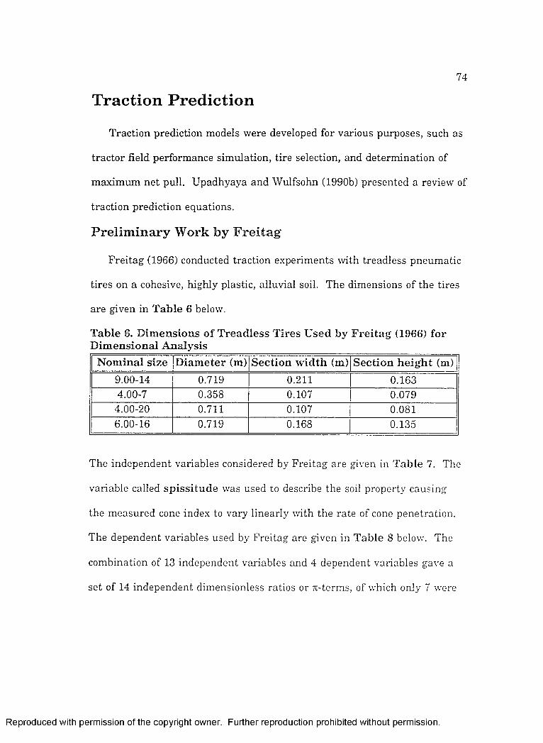
7 4
Traction Prediction
Traction prediction models were developed for various purposes, such as
tractor field performance simulation, tire selection, and determination of
maximum net pull. Upadhyaya and Wulfsohn (1990b) presented a re\new of
traction prediction equations.
P relim in a ry W ork by F re ita g
Freitag (1966) conducted traction experiments with treadless pneumatic
tires on a cohesive, highly plastic, alluvial soil. The dimensions of the tires
are given in T ab le 6 below.
T ab le 6 . D im en s io n s o f T re a d le s s T ires U sed by F r e i t a g (1966) fo r D im e n s io n a l A nalysis
N o m in a l s ize D ia m e te r (m) S e c t io n w id th (m) S e c t io n h e ig h t (m)9.00-14 0.719 0.211 0.1634.00-7 0.358 0.107 0.079
4.00-20 0.711 0.107 0.0816.00-16 0.719 0T 68 0.135
The independent variables considered by Freitag are given in T ab le 7. The
variable called s p is s i tu d e was used to describe the soil property causing
the measured cone index to vary linearly with the rate of cone penetration.
The dependent variables used by Freitag are given in T ab le 8 below. The
combination of 13 independent variables and 4 dependent variables gave a
set of 14 independent dimensionless ratios or Ti-terms, of which only 7 were
R eproduced with perm ission of the copyright owner. Further reproduction prohibited without perm ission.

10
T ab le 7. I n d e p e n d e n t T ire-Soil S y s tem V aria b le s U sed b y F r e i t a g (1966)
V a r ia b le Sym bol D im e n s io n
Soil Friction angle 4) noneCohesion c ML-'T-Specific weight y ML'^T-Spissitude P ML-'T '
Tire Diameter d LSection width b LSection height h LDeflection Ô L
System Load w MLT-Translational velocity V. L T ‘Slip s noneTire-soil friction p noneAcceleration due to gravity g LT'“
T ab le 8 . D e p e n d e n t V a r iab le s U sed by F r e i t a gV ar ia b le Sym bol D im e n s io n
Pull (net traction) P MLT-Towed force (motion resistance a t zero torque) P t MLT-Torque T ML'-T-Sinkage z L
retained for dimensional analysis. These Ti-terms are listed below and
explanations are given for the rejects.
TTi = PAV = pull number (performance number);
rco = PyW = towed force number (performance number);
K3 = T/d W = torque number (performance number);
K4 = z/d = sinkage number (performance number);
Tij = p = tire-soil friction angle, not used because friction occured between
R eproduced with perm ission of the copyright owner. Further reproduction prohibited without perm ission.

7 6
soil particles ra th e r than a t the tire-soil interface (some soil always adhered
to the wheel);
TCg = (t) = soil friction angle, not used because the clayey soil behaved like a
purely cohesive (see paragraph on Soil Properties Related to Traction);
= S = slip, not used because it was controlled, except for the towed-wheel
case;
7Ï3 = b/d = shape number;
Xg = h/d = section height to diameter ratio, not used because it could not
have a significant effect since the tires tested had similar ratios;
TCjo = 5/h = deflection number;
Ki, = c d“AV = clay loading number;
Kjo = Y d'*AV = ratio related to specific weight y, not used because the soil
was purely cohesive;
Ki3 = P dAV = ratio related to P, not used because P was proportional to
cone index, Cl;
Jti4 = g dA // = velocity ratio, not used because all the tests were conducted
a t the same velocity.
Because c was related to 01, the expression for jr,i was replaced by x,, = Cl
d ’AV. With only seven x terms left (x,, x.j, Xg, x , Xy, X;o, X;,), Freitag tried to
simplify the problem even further by looking at possible relationships
between x-terms containing independent variables only. The effect of tire
width was studied by plotting l/Xy vs. x for tires having a similar diameter
R eproduced with perm ission of the copyright owner. Further reproduction prohibited without perm ission.

7 7
but different widths (9.00-14, 6.00-16 and 4.00-20). A linear curve passing
through the origin was obtained. Therefore,
^ t (86)6 FT
where was the proportionality constant. By rearranging,
— = £ I A A . (87)
The constant term (CTb dAV) was called the c lay n u m b e r . A similar
approach was used to study the effect of tire deflection, by plotting l/niio vs.
Tc,]. This time, the equation obtained was of the form.
h5
, Cl b dfip2w
where kj.., was a constant. After rearranging.
(88)
A (89)h
These equations were then validated by comparing them with other
experimental data obtained at the USWES. The work done by Freitag
clearly influenced the experimental methodology and traction models
developed later. For example. Turn age (1972) used dimensional analysis to
modify Freitag’s clay number and to develop the equation for a mobility
number for sand similar to tha t developed by Freitag for clay. However,
R eproduced with perm ission of the copyright owner. Further reproduction prohibited without perm ission.

7 8
researchers la ter extended the use of the clay number to all soils ra the r
than pursuing Tum age’s work on sand, probably for simplification.
T raction on C oncrete
Zoz and Brixius (1979) used data from tests done a t the John Deere
Company and combined them with Nebraska test data to develop traction
prediction equations for bias plv agricultural tires on concrete. These
equations were similar to those developed earlier by Wismer and Luth
(1974). Regression was used to obtain the equations:
For the net pull (or net traction),
N T = 1.02U - e I W
For the gross pull (or gross traction),
GT = (1.02(1 - e + 0 .02) W
where:
k|{ = 400 kPa (constant relating to rubber hardness).
Tests a t the John Deere Company indicated tha t torque requirements,
which were not measured at Nebraska, could be estimated by assuming the
motion resistance MR to be equal to 2% of the d>mamic tire load W, hence
the term 0.02 in the gross traction equation. For torque calculations, the
R eproduced with perm ission of the copyright owner. Further reproduction prohibited without perm ission.

7 9
rolling radius r,j was taken as th a t on a hard surface. Consequently, wheel
tractive efficiency was computed as;
t e = (92)N T ]
[+ 0.02
Zoz and Brixius stated that, for single bias ply tires,
tire load information indicates tha t rated load (W„,^) is linearly related to tire width * diameter. For a particular inflation pressure:
= C \ 6 d ( 9 3 )
where:Cl = constant depending on inflation pressure, b = tire section width, d = tire section diameter.
The term 1.02 in the pull equations gave the maximum drawbar pull ratio
(PAV)„, .j th a t could be obtained on concrete at 15% slip as defined by the
Nebraska Tractor Tests. Actually, Nebraska tests for 1967 and 1968
showed th a t a maximum value of 1.036 could be obtained. The maximum
pull was strongly influenced by tire load and an analysis of Nebraska test
da ta showed tha t "best tire performance is obtained, both in the field and on
concrete, when the tire is not operated near its limit in regard to torque
and/or weight carrying capacity". Because tire tread bar height also
influenced performance significantly, the tire wear limit for Nebraska tests
was set a t 65% of new tire bar height. Tire manufacturer, hardness and/or
age, as well as tire construction, could influence performance. Note tha t
R eproduced with perm ission of the copyright owner. Further reproduction prohibited without perm ission.

80
"best selection for use on concrete is not necessarily the best under field
conditions". According to Zoz and Brixius, "the radial ply tire produces
significantly higher pull at the same slip and about 1 to 2 percent higher
maximum efficiency". Tire operation history also affected performance
because
high wear ra tes require high pulls and axle torques and tend to shape the lugs to an abnormal condition. Best test results are usually obtained after several hours of relatively light torque operation.
The equations developed by Zoz and Brixius assumed tire ba r height near
the 65% limit, obtained under a "somewhat optimal conditioning". Also,
"best performance is obtained with cool air and a clean track" (ambient
tem perature and track cleanliness parameters). As a summary, the
variables affecting traction on concrete were;
- tire tread bar height,
- tire manufacturer, rubber durometer hardness and/or age,
- tire construction (bias or radial ply),
- dynamic weight as related to tire size (percent of tire carrying capacity),
- tire rubber conditioning prior to test (tire operating history), and
- ambient tem perature and track cleanliness.
Effect of the number of plies was not discussed. Inflation pressure
appeared in the coefficient C, but was not discussed in detail. A double
iterative method (iteration on slip and on weight transfer) assuming motion
resistance of the front wheels to be equal to 2% of the dynamic front weight
R eproduced witti perm ission of ttie copyrigtit owner. Furttier reproduction protiibited wittiout perm ission.

8 1
(in 2WD mode) was presented. Leviticus and Reyes (1985) la ter confirmed
the validity of the choice of variables and of the traction equations.
T raction in th e F ie ld
Several m athematical models have been used to predict the performance
of tractors in the field. The purpose was to predict gross traction and
motion resistance. The most commonly used equations are presented here.
Note th a t they were developed for conventional, bias-ply tires. Researchers
then tried to adapt the models to radial tires. Most experiments agreed
th a t radial-ply tires gave better performance, in general, bu t models for
radiais required further investigation before being adopted.
Zoz T r a c t io n P r e d ic t io n C h a r t
Zoz (1972) developed a chart for two-wheel drive tractors. This chart
was included in ASAE Standard D23Û.4 (ASAE, 1989d), but it could not be
used for four-wheel drive tractors.
W ism er a n d L n t h T r a c t io n M odel
Wismer and Luth (1973, 1974) presented a dimensionless coefficient C„
called the w h e e l n u m e r ic and introduced earlier as the c lay n u m b e r by
Freitag (1966). C„ was used in the expressions for gross traction and
motion resistance, obtained through dimensional analysis.
C = (94)w
R eproduced with perm ission of the copyright owner. Further reproduction prohibited without perm ission.

GT = 0.75 (l -
8 2
( 9 5 )
M R = W L 2 + 0.04 (96)
However, Wismer and Luth recommended the following limits on their
model:
- “ 0.20 h
(97)
- “ 0.30 d
( 9 8 )
-2 » 0.475 d
( 9 9 )
Where the ro l l in g r a d iu s r^ was defined for a vehicle operated in a self-
propelled condition on a hard surface, with zero drawbar load. The model
by Wismer and Luth is used in ASAE Standard D230.4 (ASAE, 1989d)
where t}"pical values of C„ are given for drive-wheel tires with the ratio (b
dAV) close to 0.25. These values are reported in T ab le 9 below.
T ab le 9. T y p ica l AVheel N u m e r ic V alues (from ASAE S ta n d a r d D230.4)
Soil
Hard 50Firm 30Tilled 20
Soft, sandy 15
R eproduced with perm ission of the copyright owner. Further reproduction prohibited without perm ission.

8 3
G ee-C lough T ra c t io n M odel
Gee-Clough (1980) replaced C„ by another coefficient he called the
m o b i l i ty n u m b e r M, and which had been derived by Turnage (1972). He
proposed the following equations:
2 d
( 100)
'RRM R
W= 0.049 0.287
M( 101 )
where was called the co eff ic ien t o f m o tio n re s is ta n c e ,
f r ) ( 102)
where Cp was called the co eff ic ien t o f t ra c t io n ,
4.838 + 0.061 M
where was called the r a t e c o n s ta n t .
(103)
(104)
Therefore, tractive efficiency was computed as
Cj< + Cj^( 1 0 3 )
R eproduced with perm ission of the copyright owner. Further reproduction prohibited without perm ission.

84
This model was proposed as an Organization for Economic Cooperation and
Development (OECD) Standard (OECD, 1984) to predict tractor field
performance from test data. Dwyer and Heigho (1984) also gave the
following equations for the maximum tractive efficiency TE^^ and the
coefficient of traction a t 20 % slip;
T E ^ = 78 - (106)M
and,
(CtL s™..,* = 0.56 - (107)
According to Gee-Clough (1980), the prediction of ( C ; . ) , a n d Ckr was
sufficient to fully describe the tractive performance of a tire in off-road
conditions.
Dwyer, Evernden, and McAllister (1977) made a least squares regression
analysis of experimental data to obtain equations reflecting the increase in
pei-formance between the first and second passes of a same tire on the same
spot. These equations could be used to account for the effect of traffic on
field performance. The mobility nimiber used in these equations, given
below, was the one computed before traffic.
( ^ ^ 2 0 % slip , second pass _ ^ 0 . 6 2 0 ( 1 0 8 )
{ ^ 1) 20% slip, fir s t p a ss ^
R eproduced with perm ission of the copyright owner. Further reproduction prohibited without perm ission.

85
second pass _ _ 0.896 ( 109)
first pass
and
max)second pass _ -, . 0.473= 1 + ( 110)
Ç ^^m a x)fi^s t pass
B rix iu s T r a c t io n M odel
Brixius (1987) introduced another dimensionless coefficient B„, also
called m o b il i ty n u m b e r , which he used to empirically develop other
expressions for the gross traction and the motion resistance of conventional
tires.
Bn =[ h
1 b[d
( 111 )
The zero slip condition was defined as self-propelled condition (NT = 0) on a
hard surface, and rolling radius was either measured, or computed
according to the Brixius-Wismer model. Tire section height, h, was not
computed according to the definition, but as half the difference between the
overall tire diameter and the overall rim diameter. Overall rim diameter
was either measured, or estimated as 1.06 times the nominal rim diameter,
d,.i„ . Thus h could be computed as,
R eproduced with perm ission of the copyright owner. Further reproduction prohibited without perm ission.

h = d - overall rim diameter
86
( 112 )
or,
Gross traction and motion resistance were computed as,
G T = 17(0.88 (l - (1 - e^v-ss)) + o.04)
(113)
M R = W — + 0.04 0.5 S
A : j
(114)
(115)
Brixius proposed an equation to account for the change in cone index due to
soil compaction under the front axle wheels. Differences in tire number and
section width between axles were also considered:
C L = CL/1 + 1 .8
( N F T bf]2 \
g - O l l B v
V N R T brj /
where:
bf = front axle unloaded tire section width (m),
B„f = front axle mobility number,
hr = rear axle unloaded tire section width (m),
Clf = cone index before traffic (Pa),
CIr = cone index after traffic (Pa),
(116)
R eproduced with perm ission of the copyright owner. Further reproduction prohibited without perm ission.

8 7
NFT = num ber of front axle tires, and
NRT = num ber of rear axle tires.
Brixius suggested th a t S be set equal to zero in the expression for MR to
compute the motion resistance of an empowered wheel. T ab le 10 below
presents the range of field test variables reported by Brixius for tractor
tires. F ig u r e 14 shows the limits of the model proposed by Brixius.
T ab le 10. R a n g e o f F ie ld T es t V a r ia b le s U se d by B rix iu s (1987)
S o u rc eT r a c to r
d a t a ty p em b/d
M in M ax M in M ax M in M ax
NIAE 2\VD, 20% slip 4 58 0.161 0.239 0.220 0.306Deere 2WD, 0-60% slip 4 95 &088 0.305 0.250 0.581
C one Index (k N /m ^ )Applicable
° 1000 2°°° 3000 4000 5000
D e fle c t io n R atio , ^ / hApplicable
T r
W /bd (k N /m ^ ):l Applicable
0.0 0.1 0.2 0.3 0.4 0.5
0 20 40 00 80 100b / d R atio
Applicable0.0 0.2 0.4 0.6 0.0 1.0
Within P red ictable1— I Limits
_ _ Apply With CddJ R eservation
Beyond P red ictab leLimits (a f te r B r ix iu s, 1987)
F igu re 14. L im its o f traction p red iction equations for the B rix ius m odel.
R eproduced with perm ission of the copyright owner. Further reproduction prohibited without perm ission.

88
O ther T raction M odels
Upadhyaya, Wulfsohn, and Jubbal (1987 and 1989) developed equations
to predict tractive performance of radial tires. These theoretical equations
gave justification to the empirical equations commonly used a t the
University of California, Davis, in curve-fitting techniques (Upadhyaya,
1988; Wulfsohn, Upadhyaya, and Chancellor, 1988).
Wolf et al. (1992) developed a traction model for the special case of very-
hard agricultural soils, such as compacted soil or di-ied irrigated semi arid
areas, where cone index measurements and other simulation models were
not satisfactory. This model filled a gap between models for traction on
concrete, and other field traction models.
Clark (1985) studied the importance of each coefficient in the
generalized form of the Wismer-Luth model:
w(117)
w-here:
c, and Cj = constants depending on soil surface,
Cy = constant representing the maximum (NTAV) ratio, and
C7 = constant depending on soil surface and tires.
For Cl ranging between 0 and 5 MPa, Clark showed tha t the order of
decreasing importance for the coefficients was: Cg, c-, c and c . Test data
and statistical analysis were then used by Clai-k to determine optimum
R eproduced with perm ission of the copyright owner. Further reproduction prohibited without perm ission.

89
coefficients for a front-wheel assist tractor (Kubota L245DT) on three tj-pes
of soil surfaces: Short mowed grass on a soil tha t had not been disturbed
for a t least five years; tall, dense and approximately one foot high grass on
a soil undisturbed for a t least five years; and a bare soil surface disked one
m onth before the test and having received some soaking ra in since.
Coefficients c , Cg and c? were first set a t the values found in the Wismer-
Luth model to determine the optimum value of c . Then c was set to its
optimum value and c and c kept unchanged to optimize c-j. Optimum
values of Cg and c?, and unchanged value of C4 were then used to optimize Cg.
Finally, optimized values of Cg, Cg and c-j were used to optimize c .
Minimum, maximum, and step values during optimization were,
respectively:
- for C4: 0, 1.5 and 0.1
- for Cg: 0 , 0.1 and 0.01
- for Cg: 0.2, 0.9 and 0.01
- for C - : 0, 1 and 0.1
Clark found tha t the original values proposed by Wismer and Luth for c,, c-
and C7 (1.2, 0.04 and 0.3, respectively) were acceptable for net traction
prediction. Values of Cg were as low as 0.26 for the tall grass surface, 0.39
on the short grass, and 0.45 on the bare soil. Optimum values of Cg fitted
the data better for the front wheels than for the rear wheels of the tractor,
but changes in cone index due to traffic were not accounted for. Clark
R eproduced with perm ission of the copyright owner. Further reproduction prohibited without perm ission.

9 0
suggested th a t Cg was similar to the coefficient of friction between tire and
surface, and should therefore decrease as the friction coefficient decreased.
Clark also noted th a t the average cone index for the 0-15cm depth range
was not satisfactory to describe soft soil (Cl equal to 1.5 MPa or less).
Wittig and Alcock (1990) developed a single wheel tester using a small
drive wheel (Goodyear 6.7-15 Sure Grip tire inflated a t 100 kPa) mounted
behind a tractor to measure topsoil traction conditions by measuring the
maximum transferable torque for known loads. Drawbar pull tests were
run simultaneously with a Ford 8000 tractor fitted with Goodyear 18.4-38
Dyna Torque II rea r tires inflated a t 100 kPa. Cone index, soil moisture
content and bulk density were recorded. Non-linear regression analysis was
used to compare the measured tractor coefficient of ne t traction (NTAV) for
the tractor with values predicted by the Wismer-Luth model with respect to
slip. A linear relationship was found between wheel torque and dynamic
load measured with the single-wheel tester. Stepwise regression analysis
was then used to obtain a model relating the tractor net traction coefficient
to soil moisture content and bulk density, slope of the torque/dynamic load
curve, and a dimensionless number computed for each soil surface. This
number, called t e s t w h e e l n u m e r ic , was similar in meaning to the wheel
numeric C„ used in the Wismer-Luth model, but was computed, for each soil
surface, as the average maximum torque observed with the wheel tester,
divided by the product of wheel dynamic load and rolling radius, -ie.
R eproduced with perm ission of the copyright owner. Further reproduction prohibited without perm ission.

9 1
(Tn,ax/(W Cone index, and therefore C„, were rejected as traction
indicators because of the large scatter in cone index values throughout a
same soil. Tests were run on 11 different soil surfaces to generate the
model and 3 additional surfaces were used for its validation. The model
was more accurate than the Wismer-Luth model but required a more
complicated data collection system (soil moistwe content and bulk density,
and single-wheel tester results, instead of cone index alone). Effect of
dynamic load on rolling radius was not accounted for. Also, this model was
developed for a two-wheel drive tractor and its extension to front-wheel-
assist and four-wheel drive tractors was not discussed.
Evans, Clark, and Manor (1989) fitted the generalized form of the
Brixius model to experimental data. The generalized equation for gross pull
was,
GT = W(cg(l - e ‘"‘>-®")(l - + 0.04) (118)
where Cg, Cy and c,y were the regression coefficients.
The equation for motion resistance was not generalized because it fitted
data satisfactorily. Also, motion resistance was relatively small compared
to gross traction. The most significant coefficient was the slip coefficient c,,,.
When it was changed from the 7.5 value proposed by Brixius, to 3.78, the
model could predict the net traction for a small front-wheel assist tractor
(Kubota L245DT, 16.7 PTO kW) on a mowed surface covered with 5 cm high
grass. Evans, Clark, and Manor also drew contour maps showing lines of
R eproduced with perm ission of the copyright owner. Further reproduction prohibited without perm ission.

92
equal tractive efficiency as a function of front and rear axle ballast values.
They showed th a t ballast could be greatly reduced from its value a t
maximum tractive efficiency, while not losing much tractive efficiency.
Also, tractive efficiency increased more significantly when starting to add
ballast then when approaching maximum tractive efficiency. This can be
interpreted by saying th a t the more hallast is added, the harder it is to
reach maximum tractive efficiency through ballast addition. Therefore,
other techniques may be preferable when approaching maximum tractive
efficiency, especially when excessive compaction is to be avoided.
Grisso et al. (1991, 1992a) compared the field tractive performance of
18.4R46 and 18.4R42 Firestone All Traction 23" tires. The NLIN procedure
of the SAS statistical software (SAS Institute, Cary, North Carolina) was
used to fit regression curves to the data obtained. This procedure is based
on the Gauss-Newton method of non-linear regression. The 3 regression
equations used by Grisso et al. were:
F/
TE = 17 (1 -.R) (121)
where Cjj, c,2, Cjj, c, , 0,5, c,g, c, and c g were the regression coefficients.
R eproduced with perm ission of the copyright owner. Further reproduction prohibited without perm ission.

9 3
No significant tractive advantage was found for any of the two tires, which
were operated a t high inflation pressure on firm soil. The R'“ values
obtained for the first 2 regression equations showed good agreement
between predicted and measured values but they were not as satisfactory
for the TE prediction equation.
Bashford et al. (1993) used the same model as Grisso et al. (1991) under
the NLIN procedure of the SAS software to study the dynamic traction ratio
(PAV) and tractive efficiency TE of a tractor equipped with three different
size Firestone Radial All Traction 23“ rear tires (1S.4R42, 18.4R46 and
12.4R54). Three levels of inflation pressure (55 kPa, 83 kPa and 124 kPa)
and 2 types of soil surface (wheat stubble and plowed wheat stubble)
provided the various operating conditions. The computed regression
coefficient estimates and 95% confidence intervals for these coefficient
estimates were given for each test case. R‘~ values for dynamic traction
were all above 0.93. Regression fits were not as good for tractive efficiency,
with R" values as low as 0.27. None of the tires appeared to prow de
significantly better performance for all conditions. In general, tractive
performance increased when inflation pressure decreased. The size of the
tractor front wheels seems to have affected the results, thus making it
difficult to study the effect of overall diameter.
Attempts were also made to extend the models presented above to a
larger range of tires. Ashmore, Burt and Turner (1987) successfully
R eproduced with perm ission of the copyright owner. Further reproduction prohibited without perm ission.

9 4
modified the Wismer-Luth model to predict performance of log-skidder tires
in the NSDL soil bins. McDonald, Stokes, and Wilhoit (1992, 1993)
proposed an empirical equation derived from the Wismer-Luth model and
fitted it to field da ta obtained from a log-skidder. The curve fitting method
used the NLIN procedure of the SAS software. The empirical equation was,
— = c , g (l - e (122)
where:
So = constant accounting for the error in slip measurement;
Ci9 and c.,0 = regression coefficients.
A total of four different log-skidder tire sizes were tested both under road
(haul road) and field (forested surface) conditions, and six different tire sizes
were tested on road conditions. Computed coefficients were given as well as
R" values, which were all above 0.91. McDonald, Stokes, and Wilhoit found
no apparent relationship between tire width and net traction as a function
of slip for the tire conditions tested. Radial-ply tire performance was not
affected significantly by the test surface, while bias-ply tire performance
was. McDonald, Stokes, and Wilhoit (1992) also used the model developed
by Upadhyaya, Wulfsohn, and Jubbal (1989) to derive a regression equation
for tractive efficiency. Net and gross traction ratios were represented as
(Upadhyaya, 1988; Wulfsohn, Upadhyaya, and Chancellor, 1988;
Upadhyaya, Wulfsohn, and Jubbal, 1989),
R eproduced with perm ission of the copyright owner. Further reproduction prohibited without perm ission.

9 5
^ = c , (l - (123)W
= (%,(! (124)
and,
GT W
where c i, c g, Cgg, Co and were the regression coefficients. Coefficients c.,o
and Cg5 were assumed to be identical because they were both related to
shear stress a t the soil-tire interface. Therefore,
Co (l -T E = — {1 - S) (125)
c%; ^
Approximating the exponentials as the zero and first terms of their Taylor
series expansions,
TE = ^ C22 S a - S) (126)^23 1 " ^24 (1 “ *^22 ^
Using the properties of the various coefficients McDonald, Stokes, and
Wilhoit derived an equation to compare tractive efficiency between single
and dual tires,
_ <^22s(l ^24d (1 ^22d (127)^22d (1 " ^2As (1 ^22s
where the s and d subscripts referred to the single and dual tires,
respectively. McDonalds, Stokes, and Wilhoit then used this equation to
R eproduced with perm ission of the copyright owner. Further reproduction prohibited without perm ission.

96
explain why they observed better tractive efficiency for single tires than for
duals in their experiments.
C om puter S im u lation and D ec is io n A ids
Kotzabassis et al. (1987) developed a simulation model based on
Wismer-Luth (1974) equations. In-soil tractor performance was predicted
only a t rated engine load and speed. Kotzabassis and Stout (1989) then
developed a tractor-implement interaction model called ISTP (In-Soil
Tractor Performance), which used Brixius (1987) traction prediction
equations. Through iterations, this model balanced the power demand on
the implement hitch with the available axle power. Performance in either
2WD or 4WD mode could be predicted, and the increase in cone index
caused by the front tires was accounted for in the rear axle performance
computations. On-concrete Nebraska Test results were stored in a database
and used as inputs to the model. Kotzabassis, Stout, and W hittaker (1989)
also developed a software package for farm machinery management. A
tractor-implement matching expert system was written in PROLOG
language to schedule fai-ming operations by crop and by month, according to
tractor field performance, implement information, farm description, crop
schedules and weather probability.
Brassart (1989) developed and combined a FORTRAN traction
simulation program with a dBase III Plus database management system to
facilitate the selection of agricultural tractor tires. Combinations including
R eproduced with perm ission of the copyright owner. Further reproduction prohibited without perm ission.

9 7
a tractor, an implement, a set of tires and soil conditions could be
assembled easily and simulations could be made to study the effect of the
selected tires on tractor tractive performance for given soil conditions and
farming operations. The simulation program, based on Brixius (1987)
equations, accounted for changes in cone index after traffic by the front
axle, weight transfer, tire number (single or dual) and ballast to give
recommendations to optimize tractive efficiency. A significant feature of the
simulation program was th a t slip was not considered as an independent
(preselected) variable as in most previous simulation programs. Instead,
slip was iteratively computed to accomodate tractor available axle power to
implement draft.
Other simulation programs were written for various tractive
performance prediction purposes, a num ber of them using Wismer-Luth
(1974) equations (Macnab, Wensink, and Booster, 1977; Iff et al., 1984;
Alimardani, Colvin, and Marley, 1989). Summers and Von Bargen (1983)
and Summers, Ekstrom, and Von Bargen (1986) combined traction
equations with a Lagrangian method to account for kinetic and potential
energy in a tractor’s driveline. Their model was validated by comparing
simulation results with Nebraska Test reports. Mussel, ShmuleVch, and
Wolf (1992) developed an iterative program based on soil-tire interface
stresses and soil constitutive relationships to simulate traction. A
particular feature of the program was tha t it accounted for the phenomenon
R eproduced with perm ission of the copyright owner. Further reproduction prohibited without perm ission.

98
of rolling resistance decrease with increasing travel speed, as observed
earlier by Pope (1971).
Zoz (1987) presented a computerized spreadsheet method to refine and
replace the chart developed previously (Zoz, 1972). The Lotus 1-2-3
template used equations developed by Brixius (1987) for field performance
prediction, and equations proposed by Zoz and Brixius (1979) to predict
performance on concrete of tractors mounted with bias-ply tires. Tire
dimensions selection and PTO/axle efficiencies for both axles were required
among the inputs. Several options were offered, such as calculations for a
concrete surface or field soil, for two-wheel drive or four-wheel drive (or
mechanical front-wheel assist), with an emphasis either on performance
(tractive efficiency and drawbar pull), or on dynamic weight distribution of
the tractor. Tire dimensions and load capacities were selected from a
lookup table included in the program. Only the highest ply rating (load
capacity) tires of each size were stored in the original table, but additional
data could be entered. For field-performance simulation, values of 1800,
900 and 450 kPa were used as typical soil cone index values for good,
medium and poor tractive conditions, respectively.
Al-Hamed et al. (1990) amended this spreadsheet program according to
recommendations made by Brixius (1987) to accomodate radial tires, and to
include a ballast optimization scheme. Optimum weight distribution was
computed either from the maximum tractive efficiency case, or from the
R eproduced with perm ission of the copyright owner. Further reproduction prohibited without perm ission.

9 9
design tractive efficiency case (3 % slip above the slip value a t maximum
tractive efficiency). The generalized form of the Brixius model was used:
G T = W (0.88 (1 - e-o-i (l -
N T = W 0 . 8 8 (1 - e - o i - B n ) (2 - ^Bn
M R = W ‘'28 + C.27 + 0.5 S]
(128)
(129)
(130)Bn “■ ^
where c g, c-i? and c,g were traction coefficients based on tire type (radial or
bias-ply construction) as given in T ab le 11.
T a b le 11. C oeff ic ien ts U se d b y A l-H am ed e t al. (1990) in B rix iu s T r a c t io n M odel
T r a c t io nco e ff ic ien t
T i re typeb ia s -p ly ra d ia l-p ly
7.50 &50C.27 0.04 ff03223 1.00 ff90
Evans, Clark, and Manor (1989) used another generalized form of the
model because they were interested in soil surface effects. Later, Evans,
Clark, and Manor (1991) included surface condition effects in a traction
model they used to help farmers optimize ballast combinations by drawing
tractive efficiency contour maps with front and rear axle ballast as entries.
Grisso et al. (1992a) also used a modified version of the Zoz (1987)
spreadsheet templates to show the effects of tire construction (bias vs.
radial), tire number (single vs. duals), travel speed, tire size, ballast
R eproduced with perm ission of the copyright owner. Further reproduction prohibited without perm ission.

1 0 0
distribution, soil condition and drive mode (2WD vs. 4\VD or FWA) as an
educational tool for students in undergraduate classes and farmers. They
used non conventional variables to better describe tractor tractive
performance (see paragraph on "Other Performance Criteria").
Ramp and Siemens (1990) proposed a program matching tractors with
implements to obtain maximum productivity and best use of tractor
available power. The program was based on Brixius traction prediction
equation and accounted for incremental ra ther than continuous increases in
implement sizes. The implement giving the highest draft without exceeding
tractor maximum pull for a chosen gear ratio was retained as a possible
match. Several gear ratios were tested, and the corresponding implement
size, slip and productivity values computed. The combination giving the
highest productivity could then be selected.
Downs, Taylor, and Al-Janobi (1990) developed an expert system to
match ballast, implement size, drive tires and tire inflation pressure
according to soil conditions. In the first part of the program, front and rear
tractor static weights were obtained from a tractor and tire database. Then
the user had to specify any additional weight: iron weights on axles, dual
tires, and water or CaCL in the tires. Axle static load distribution could be
modified by entering other values for the static axle weights. Operating
speed, slip and soil cone index information was then requested. Tables were
R eproduced with perm ission of the copyright owner. Further reproduction prohibited without perm ission.

1 0 1
displayed to help provide estimates for cone index and slip. These tables,
which were derived from ASAE Standards D230.4 (1989d) and EP391.1
(1989c), are shown below (Tables 12 and 13). For comparison purposes,
T ab le 14 below shows the ranges of slip given in ASAE Standard EP391.1
(1989c) to obtain maximum tractive efficiency.
T ab le 12. E s t im a te s o f C one In d e x A c c o rd in g to Soil C o n d i t io nSo il c o n d i t io n C one in d e x (k P a)
hard, packed 1724hard, packed with stubble 1379
firm 1034tilled 552
soft, wet 414
T ab le 13. E s t im a te s o f O p tim u m S b p A c c o rd in g to T r a c to r D riv e T ype a n d Soil
Soil ty p e IV a c to r d r iv e type2\VD FWA o r 4’VVD
firm 10-1 2 '% 8-10 %tilled 12-14 % 10-11.5 %sandy 14-16 % 11.5-13 "%
The ballast program provided recommendations such as:
- Reduce front or rear axle weight if maximum tire load was exceeded, or
suggest a change in tire size,
- Reduce ballast if the tractor was two-wheel drive and the total
weight/horsepower ratio was over 895 N/PTOkW, or
- Reduce weight if the tractor was four-wheel drive or front-wheel assist,
and total weight/horsepower ratio was over 835 N/PTOkW.
R eproduced with perm ission of the copyright owner. Further reproduction prohibited without perm ission.

102
T able 14. O ptim um Slip R anges for M axim um TE A ccord in g to Soil T ype (ASAE Standard EP391.1)
S o il typ e Slip range (%)concrete 4 - 8firm soil 8 - 10tilled soil 11 - 13
soft soils and sands 14 - 16
These recommendations implied a total tractor dynamic weight to
horsepower ratio between 597 and 835 N/PTOkW for a four-wheel drive or
front-wheel assist tractor, and between 716 and 895 N/PTOkW for a two-
wheel drive tractor.
The second part of Down, Taylor, and Al-Janobi’s program matched
implement size to tractor power. Optimum dynamic tractor weight was
arbitrarily defined to be 746 N/PTOkW for a four-wheel drive or front-wheel
assist tractor, and 835 N/PTOkW for a two-wheel drive tractor. Two series
of estimates were made based on current tractor weight and on optimum
tractor weight. Each series contained three estimates:
- Tractor speed and slip at a given drawbar pull,
- Tractor speed and drawbar pull at a given slip, and
- Drawbar pull and slip a t a given indicated speed.
Typical values of implement draft were displayed to help the user provide a
draft estimate (T able 15).
R eproduced with perm ission of the copyright owner. Further reproduction prohibited without perm ission.

1 0 3
T able 15. D raft E stim ates A ccord in g to Im plem ent TypeIm plem ent D raft, kN/m of im p lem en t w id th
moldboard plow 7.983chisel 3.911
chisel with sweeps 3.692tandem disk 4.043
offset disk 3.663V-blade 4.510
The tractor was assumed to be loaded a t 75 % of full load (tractor maximum
pull = draft/0.75) to compute front and rear axle dynamic loads, and slip.
Draft angle was also set to zero for towed implements connected to the
drawbar. Zoz equations (1972) were used to compute weight transfer and
axle dynamic loads. Bri.xius model (1987) was used to compute slip. The
third part of the program used data and results from the previous two parts
to provide tire size and inflation pressure recommendations, based on ASAE
Standard S430 (1989e). Tire lug type (general, high lug, or industrial) was
selected according to soil conditions. Ballast was then optimized. For
computations, the drawbar power/PTO power ratio was estimated by using
T ab le 16 below.
T ab le 16. R a t io o f D ra w b a r P o w e r to PTO P o w e r A c c o rd in g to Soil C o n d i t io n a n d T r a c to r D riv e T ype
T r a c to r d r iv e Soil typety p e C lay M ed iu m Soft2\VD 0.72 0.67 0.55FWA 0.77 0T3 (1654WD 0T 8 0.75 ff70
R eproduced with perm ission of the copyright owner. Further reproduction prohibited without perm ission.

1 0 4
For tire size selection, the program assumed the maximum drawbar load
equal to 45 % of the rear axle load. For dual tires, the dynamic load on the
tires was set equal to the axle load divided by (4 x 0.88) to satisfy ASAE
Standard S430 (ASAE, 1989e) for dual tire loads. If necessary, tire pressure
was computed through linear interpolation on values given in ASAE
Standard S430, which also provided a value for the minimum inflation
pressure. Additional rules were inserted in the expert system to assist tire
selection;
- Tire replacement was not recommended as long as lug height was larger
than 20 % of the original height. Tire condition was otherwise described by
four categories: new, good, poor, and worn;
- Radial tires were not recommended in sandy and wet soils;
- Radial tires performed better than bias tires on tilled and firm soil;
- Dual drive tires were recommended for two-wheel drive tractors of 104
PTOkW (140 PTOhp) and above;
- Dual tires were recommended for front-wheel assist and four-wheel drive
tractors to carry tractor weight and reduce compaction;
- High-lug tires were recommended if the tractor was used 40 Tc or more of
the time in muddy (tight or sticky soil) areas and 20 % or less in hard
(roads or hard soil) areas;
- Industrial tires were recommended if the tractor was used 60 % or more of
the time in hard areas and 20 % or less in muddy areas;
R eproduced with perm ission of the copyright owner. Further reproduction prohibited without perm ission.

1 0 5
- General purpose tires were recommended whenever the above rules did
not apply;
- Dual radial tires were not recommended for most conditions because of
cost and limited performance improvement;
- Compaction problems were minimized by reducing ballasting weight or
using dual tires;
- Tire configuration (duals or single) was based on rear axle load.
Other models were derived from Gee-Clough’s model. Gee-Clough et al.
(1978) proposed a model combining traction equations to implement draft
equations to predict field productivity of tractor-implement combinations for
plowing operations in particular. Based on data collected at the NIAE,
Dwyer (1978) presented methods to maximize performance by matching
tractor weight, tire sizes and travel speed to the available power.
E rada t Oskoui, Witney, and Voorhees (1990) built an expert system to
assist farmers in managing machinery with regard to factors such as
compaction, timeliness penalties (ie, reduction of jaeld and crop marketing
opportunities due to non optimization of field operation timing) and field
work productivity as affected by tractive efficiency, and implement size and
draft. The Gee-Clough model was used for traction prediction in the
identification of tractor-implement combinations suitable for a given field
operation, and a particular soil type under specified climatic conditions.
R eproduced with perm ission of the copyright owner. Further reproduction prohibited without perm ission.

1 0 6
Other models were included in the expert system to estimate soil moisture
content, cone index, and implement draft.
Marquez (1980) developed a program to predict tractor drawbar
performance on paved track by using PTO test results. Objectives of this
research were to reduce the num ber of costly official track tests by
predicting their results from PTO tests, and to insure a greater homogeneity
among test results.
Because field productivity of agricultural machinery also depended on
engine performance, mathematical models of tractor engine performance
were developed (Harris and Pearce, 1990; Harris, 1992a) and the use of
standard PTO tests was suggested to determine regression coefficients
associated with each type of engine (Harris, 1992b; Jahns, Forster, and
Hellickson, 1990). These models could be combined with traction models
and implement draft models to form complete simulation programs.
Lima, Souza, and Milanez (1992) proposed an empirical model using
polynomial functions to represent the overall efficiency of a tractor in the
field. This method was proposed initially by de Souza and Milanez (1991) to
predict tractor performance on concrete. Kolozsi and McCarthy (1974) also
proposed a model to predict tractor field performance from a set of tests
encompassing both concrete and field surfaces. This type of model b_vpassed
the problem of finding an adequate traction model, but also prevented
comparisons of performance prediction based on tire characteristics, such as
R eproduced with perm ission of the copyright owner. Further reproduction prohibited without perm ission.

1 0 7
tire dimensions or carcass construction. Enough performance data in
various soil surface conditions had to be collected before interpolations could
be made for other surfaces. Kolozsi and McCarthy used no quantitative
variable to characterize the soil surface, bu t only a qualitative description,
which limited the accuracy of their model.
Soil B e h a v io r an d Soil-T ire In te ra c tio n s
Scientists and engineers have tried to better understand stress
distribution both in the soil underneath a tire and a t the tire-soil interface.
Several authors presented reviews on soil compaction research (Chancellor,
1977; Soane et al., 1981a; Soane et al., 1981b) and on soil-tire interaction
models (Plackett, 1985). Chancellor made a state-of-the-art report on soil
compaction caused by agricultural equipment. The principal phenomena
observed by other researchers were presented in conjunction with
experimental data, as an educative tool to be used in an effort to
understand and reduce soil compaction. Soane et al. (1981a) discussed soil
characteristics and properties related to compaction: dry bulk density,
porosity, permeability and diffusivity, strength, cone resistance, shear
strength, surface bearing strength, surface and subsurface deformations,
stress distribution, clod and aggregate characteristics, and texture analysis.
Various approaches used in predicting compaction under wheels were also
presented: the Mohr-Coulomb theory, the Terzaghi-Prandtl theory, the
classical compression theory, the Boussinesq-Sohne theory, the Bernstein-
R eproduced with perm ission of the copyright owner. Further reproduction prohibited without perm ission.

108
Bekker theory, and critical state soil mechanics. Soane et al. (1981b) also
presented various parameters a fleeting soil compaction. These included
wheel load, tire-soil contact pressure, wheel slip, tire dimensions, carcass
construction, inflation pressure, forward speed, and number of passes.
W heel S in k age and Soil D eform ation
A traveling wheel causes both vertical and horizontal deformations on
deformable soil. The vertical deformation is due to the load on the tire and
is called s in k ag e . The horizontal deformation is principally due to the
input torque applied to the wheel. If the sinlcage value is different between
the front and rear axles, the tractor is not level, and the equilibrium of
forces is modified. This affects the efficiency of the tractor. However, it is
generally considered tha t sinkage remains so small th a t it does not have a
significant influence on tractive efficiency.
Mclfibben and Green (1940) buried small color-coded beads in Des
Moines molding sand, forming 61 mm X 61 mm squares every 61 mm in
depth. Location of the beads was carefully recorded before a 6.00-16, 4 ply
implement tire and a 152 mm width, 711 mm diameter steel wheel were
rolled across the soil bin under various load and tire inflation pressure
conditions. The new location of the beads after traffic was recorded while
removing the sand by means of a small trowel and a vacuum cleaner. This
enabled McKibben and Green to describe the movement of soil particles
under traffic for the various conditions tha t were imposed. Unfortunately,
R eproduced with perm ission of the copyright owner. Further reproduction prohibited without perm ission.

1 0 9
this technique was not applied to powered wheels. Other tests were used to
measure the effect of the number of passes in a field track on average and
maximum ru t depth, and to measure the amount of soil material adhering
to the wheels according to soil conditions.
Gamma rays were used by Khamidov (1961) to visualize the way soil is
compressed under tractor wheels. Lead balls having a diameter of 6 to S
mm were buried in the soil every 40-50 mm down to a depth of 200-300
mm. The initial location of the balls in the vertical plane was recorded by
sending gamma-rays through the soil to expose X-ray films th a t were placed
in a trench parallel to the plane of the lead balls. Then a tractor was
driven with no load over the zone of the beads and their final location was
recorded by exposing X-ray films to the Gamma rays again. Comparison of
the two recordings showed the displacement of the beads and, thus, the
deformations of the soil. The same test was run with a tractor operating
with a drawbar load. Other tests were done to compare the effects of the
driving wheels and of the unpowered ones. Ivhamidov observed tha t
unpowered wheels caused a forward horizontal motion of the beads. Self-
propelled wheels (driven wheels with no drawbar pull) only caused a
vertical downward displacement. Driven wheels with a drawbar load
caused both a backward horizontal motion and a vertical downward motion.
The combination of the effects of the front (unpowered) and the rear (driven)
R eproduced with perm ission of the copyright owner. Further reproduction prohibited without perm ission.

1 1 0
wheels was also shown by analyzing the trajectories of the lead balls in each
case. F ig u r e 15 is a schematic of the deformations observed by Khamidov.
W: dynamic load on the wheelT: wheel input torqueR: soil reactionNT; net tractionTF: towed force POWERED
WHEEL
d ir e c t io n o f tr a v e lNT
TOWEDWHEEL
d ir e c t io n o f tr a v e lTF
F igu re 15. Soil deform ations un der p n eu m atic w h eels (K ham idov, 1961).
Several authors proposed models for sinkage prediction. Bekker (1960)
mentioned the following equation (often called the Bernstein equation) to
express sinkage:
(131)
where:
p . = normal average contact pressure,
kg = soil stiffness constant,
R eproduced with perm ission of the copyright owner. Further reproduction prohibited without perm ission.

I l l
n = soil constant, and
z = depth of sinkage.
This equation was said to describe sinkage with enough accuracy for
motion resistance prediction and was used by several other authors, such as
Dwyer, Comely, and Evernden (1974), Perdok (1978), Barnes et al. (1971),
and McKyes (1985).
The constants kg and n were determined for a particular tire-soil
combination from a logarithmic plot of z vs. p ,„. F ig u r e 16 shows an
example of sinkage versus pressure curve.
(log. sca le )
PP P CO0 0 2COl(log. scale)
z: sinkage depth co n ta c t pressure
F ig u r e 16. B e k k e r p re s su re - s in k a g e cu rve .
Researchers have tried to relate sinkage to load, instead of contact
pressure, because the use of contact pressure required knowledge of the
R eproduced with perm ission of the copyright owner. Further reproduction prohibited without perm ission.

1 1 2
contact area for any load. The characteristics of both the tire and the soil
had to be known (stiffness of the tire, and strength of the soil). However,
the contact surface between a pneumatic wheel and the soil proved very
difficult to determine in practice. Consequently, all the models and
equations found, so far, have failed to describe this particular phenomenon
accurately enough to be generally applicable.
Various param eters were identified that affect sinkage. Among these
were soil strength, soil moisture content, load distribution, and ra te of
application of the load. Stafford and de Carvalho Mattos (1981) used
laboratory simulation to study the effect of hydrostatic compression pulses
(square wave) on cylindrical soil samples. Loading duration had a
significant effect on the compaction of drier soils under isotropic loading
conditions, bu t not on wet soils. The action of the wheel on the soil was
treated as a pulse wave because the load application on a given soil surface
area depended on the speed of forward motion of the tractor. Field
experiments showed tha t wheel speed affected soil compaction over a wide
range of moisture contents. This was explained by the shear action
involved in the interaction between the soil and a driven wheel (rather than
a towed one), particularly at high slip. The most important observation was
th a t shear s tra in caused more compaction a t low speed than at high speed,
because shear strength increases \rith strain rate. Pope (1969) also studied
the effect of sinkage rate on soil resistance. Because sinkage rate depended
R eproduced with perm ission of the copyright owner. Further reproduction prohibited without perm ission.

1 1 3
on wheel travel speed, the latter was recognized as having a significant
effect on motion resistance.
S o il P ro p er tie s R ela ted to T raction
Soil properties related to traction and their measurement have been
presented by numerous authors (Janosi, 1960; Osman, 1964; Gill and
Vanden Berg, 1968; Bekker, 1969; Yong, Fattah , and Skiadas, 1984; Okello,
1991). The most commonly used variables were friction, cohesion, and cone
index.
F r i c t io n a n d C ohes ion
Bekker (1960) used the Coulomb equation to express the maximum
th ru s t (horizontal force) tha t could be obtained on a given soil. In practice,
the maximum th rus t was identified with the force required to shear the
ground along the ground contact area. It was the maximum horizontal load
(or pull) th a t could be obtained for a given vertical load.
H = A c + IV tan((j)) + d 3 2 )
where:
A = ground contact area (projection on the horizontal plane of the
tire-soil contact area),
H ’ = additional shearing force produced by the tire tread and added
for better accuracy,
c = cohesion coefficient of the soil, and
(J) = friction coefficient of the soil.
R eproduced with perm ission of the copyright owner. Further reproduction prohibited without perm ission.

1 1 4
H ’ usually being a small percentage of H, the equation was reduced to:
H = A c + W tan(({)) (133)
To illustrate the meaning of c and <{), Bekker distinguished purely frictional
soils and purely cohesive soils from average soils. For soils like wet clay or
snow, the forces are mainly cohesive ones binding soil grains. These forces
were practically independent of outer pressure. Consequently, the th rust
th a t could be obtained was independent of the vertical load, and:
H = A c (134)
For purely frictional soils, like sand, no cohesion existed between the grains,
so th a t the th ru s t was only dependent on the vertical load:
H = W tan(4)) (135)
Actually, most of the soils presented a combination of both frictional and
cohesive properties, as illustrated in F ig u r e 17.
Soil S t r e n g th
Soil s trength affects sinkage, gross traction and motion resistance. A
convenient way to estimate soil strength was developed through the
m easurem ent of C one In d e x C l (expressed in Pa), because it was simple,
quick to measure, and indicative of tractive performance possibilities
(Dwyer, Comely, and Evernden, 1974). In situ measurements of Cl consist
of pushing a metallic cone tip vertically into the ground at a constant speed.
The size of the cone tip and the test procedure were standardized in ASAE
R eproduced with perm ission of the copyright owner. Further reproduction prohibited without perm ission.

1 1 5
cohesive soil frictional soil average soil
cA
W: vertical load H: gross traction
(thrust, or gross pull)
F ig u r e 17. C o h e s iv e a n d f r ic t io n a l c h a r a c te r is t ic s o f s o i ls .
Standard 8313.2 (ASAE, 19890. The force required to push the cone down,
recorded a t various depths, represents the strength of the soil at the
corresponding depth. Cone index has been used in many traction prediction
models. Some typical values of 01 were given in ASAE Standard D230.4
(T able 12). These values were recommended for not highly compactible
soils and for tires operated a t inflation pressures producing deflections of
approximately 20% radially of the undeflected tire section height (o-'h - 0 .2 ).
Brixius (1987) reported other typical values (Table 17).
Because wheel traffic modified soil conditions, mostly through soil
compaction, it was known to affect cone index significantly. Authors agreed
on the importance of the first few tire passes in reducing rolling resistance
R eproduced with perm ission of the copyright owner. Further reproduction prohibited without perm ission.

1 1 6
Table 17. Typical Cone Index Values (Brixius, 1987)Soil class Cl (kPa) Typical operating conditionsFirm soil 1750 US summer plowing; logging in dry
season; earthmoving on dry, clay soilMedium or tilled soil 1200 Great Plains, wheat harvest
1000 Corn Belt harvesting; fall plowing850 Planting; field cultivating
Soft or sandy soil 700 Spring plowing; earthmoving on moist soil
480 Disking on plowed ground; low-land logging
350 La. and Gal. rice harvest
and increasing tractive efficiency (Taylor et al., 1982), and repeated loading
was studied in the laboratory (Johnson, Bailey, and Cakir, 1992) to explain
the phenomenon observed in the field. Pitts and Goering (1979) studied the
effect of traffic on cone index using similitude. Cone index before traffic,
wheel slip, travel velocity and normal load were found to significantly affect
cone index changes. Nineteen theoretical models were tested against
experimental data and evaluated according to simple criteria. The model
finally selected did not account for slip because of the difficulty in predicting
the effects of this variable. The ratio between cone index before traffic and
cone index after traffic was given as:
Ç 4c i ,
1 + 18TB IT _o,585
CL b dg b,l (136)
where:
R eproduced with perm ission of the copyright owner. Further reproduction prohibited without perm ission.

1 1 7
CIr = cone index after traffic (Pa), and
Clf = cone index before traffic (Pa).
The criteria were: An initially loose soil was to show a low CI value and a
high CiyCIf ratio, ie. a large variation in Cl, compared to an initially hard
soil, where, as Clf increased. Cl,, had to tend toward Clf (little or no Cl
change on a hard soil); The change in Cl had to decrease with increasing
load application rate, and with increasing wheel travel speed; The effect of
wheel load was not supposed to disappear if travel speed or slip was
reduced to zero.
Dwyer, Evernden, and McAllister (1977) and Brixius (1987) used other
models to account for the effect of preliminary traffic on tractive
performance (see field traction prediction models hy Gee-Clough and
Brixius).
S o i l S t r e s s D i s t r i b u t i o n U n d e r a P o i n t L o a d
Researchers also tried to develop less empirical methods to predict soil
behavior. The theory of elasticity was modified to account for the inelastic
behavior of agricultural soils, and numei’ical methods were developed to
determine stresses and strains for the unusually large deformations
encountered. Some of the theories and methods used are presented below to
show the complexity of the problems, and the approaches used.
Das (1983) reported the Boussinesq equations for stresses inside an
elastic half-space under the effect of a point load acting on the surface.
R eproduced with perm ission of the copyright owner. Further reproduction prohibited without perm ission.

1 1 8
These equations were obtained by the method of potentials, or Airy
functions. Figure 18 below shows the axis conventions taken for these
equations.
V ertica l fo rce only H orizonta l and v ertica l fo rc e s com b in ed
F ig u r e 18. Soil s t r e s s c o o rd in a te system .
E ffec t o f a V e r t ic a l P o in t L o ad
The soil is assumed to be a homogeneous, isotropic, linearly elastic half-
medium. The point load is acting on the surface.
- In c a r t e s i a n c o o rd in a te s (Timoshenko and Gooclier, 1982; Das, 1983):
(137)
8Q2 k
x^z ^ l - 2v (2 [/+z)z-+ 2 “ U '
(138)
R eproduced with perm ission of the copyright owner. Further reproduction prohibited without perm ission.

^ l - 2v f 1 @l7+zb^ z j )2tz 3 [U[U*z) u V )
' :cy =3Qf xyz 2t ï( Î/5
l-2 v {2U-+z)xy3 UHU+zf j
T =XZ 27T
3Qyz22 %
where:
1 1 9
(139)
(140)
(141)
(142)
Q = point load,
U = radius from point of application of Q, to point considered,
V = Poisson ratio, and
(143)
where:
U =(144)
- In c y l in d r ic a l c o o rd in a te s :
Using the following transformation, where cp is the angle between the
vertical direction and the line joining the point of application of Q to the
point considered.
z - U cos(<p) (143)
R eproduced with perm ission of the copyright owner. Further reproduction prohibited without perm ission.

Then the stress equations become;
1 2 0
3 Q cos ((p) 2 TZ u-
( 1 4 6 )
Q2 7t [7= U {U + z)j
3 Q cos((p) 2
(147)
o , = ^ (1 - 2 v )[ / ( [ / + z)
=3 z% 2 TZ
or, as proposed by Feda (1978):
( 1 4 8 )
( 1 4 9 )
Q2 % z 2
3 cos ((p) sin"((p) - (1 - 2v)——-1 + cos{(f>))
(150)
= (1 - 2v) Q71 Z‘
C0s‘ ((p)
1 + cos(<p)COS ((p) (151)
E ffec t o f a H o r iz o n ta l P o in t L o a d
Das (1983) reported the stress equations proposed by Cerruti for a
horizontal load acting on the surface of a homogeneous, isotropic, linearly
elastic half-space.
- In c a r t e s i a n c o o rd in a te s (Das, 1983):
If the load is in the x direction,
(152)
R eproduced with perm ission of the copyright owner. Further reproduction prohibited without perm ission.

1 2 1
Q x2 n
Q i
[EL:: _ a _ 2v) . 0_:_2vX7!'I f / “ (cr + z)2
3 -[/= ([/ + z) Jj
(153)
2 u 1/3SLz! _ 0 _S!v) + (1 -
I 1/2 ( # +
3 _ y 2 (3 17 + z ) W l 5 4 )
([/ + z) 1
=Q y
2 n [/33 (1 - 2v)[/2
I [ / : ( # +
(3 [/ + z)(72(# + ^
^ 3 Q x ^ z 2 u Ï/3
/ /
(135)
(156)
~yz3 Q X y z (157)
2 t: f/3
Stresses for point loads applied in other directions can be determined by
simply permuting the variables x, y and z, or by applying the necessary
rotation.
- In cy lin d rica l coordinates:
The same transformation as before can be used to find the stress
equations in cylindrical coordinates.
S tre s s d i s t r ib u t io n in A g r ic u l tu ra l Soils
Actually, agricultural soils present different stress distributions when
compared with the medium assumed by Boussinesq.
- FroM icli con cen tra tion factor:
Stresses tend to be higher under the loading area than predicted with
R eproduced with perm ission of the copyright owner. Further reproduction prohibited without perm ission.

1 2 2
the Boussinesq and Cerruti equations. Soehne (1958) described this
phenomenon as follows:
The compressive stress in the soil has a tendency to concentrate around the load axis. This tendency becomes greater when soil becomes more plastic due to increased moisture content and when the soil is less cohesive, for instance sand.
Therefore, Frohlich (1934) modified the Boussinesq and Cerruti equations,
which became, in cylindrical coordinates (Johnson and Burt, 1990):
For a vertical load:
O = .9 . cos(-^((p) (158)
where m is the Frohlich stress concentration factor (m > 3).
For a horizontal load:
g = m Q sin('"-^)((p) cos(6) (15g)2 %
where 0 is the angle between the direction of the load and the projection on
the horizontal plane of the line joining the point of application of the load to
the point considered. When m = 3, these equations are the Boussinesq and
Cerruti equations, respectively. Soehne (1958) recommended m = 4 for hard
dry soil, m = 5 for soil with normal density and water content (medium
soil), and m = 6 for wet soil (soft soil).
Combining a vertical load and a horizontal load (superposition method)
provided the general equation used by Johnson and Burt (1990):
o „ =m (V cos '" 2'((p) + H sin^'" " ccs(0)) (160)
R eproduced with perm ission of the copyright owner. Further reproduction prohibited without perm ission.

1 2 3
where;
H = horizontal component of the load, and
V = vertical component of the load.
This method was based on the assumption th a t all the forces (vertical and
horizontal components) were acting on a horizontal area located at the soil
surface level and limited by the tire footprint, ra th e r than a t the actual soil-
tire interface.
Carpenter et al. (1985) used Soehne’s equations to study the effect of
wheel load on subsoil compaction, subsoil being considered as the soil below
plowing depth. They showed tha t subsoil stresses could be very high,
despite low ground pressures, because of high loads concentrated on
somewhat limited areas. They recommended the use of tracks or tandem
tires ra the r than duals or wide section tires.
- V ariable P o isso n ratio and Y oung’s m odulus:
Raper and Erbach (1990b) studied the effect of Young’s modulus and
Poisson’s ratio on stress values predicted using finite element methods.
They showed th a t the soil vertical stress beneath the center of a flat
circular plate was dependent on Poisson’s ratio, and tha t soil s tra in was
dependent on both Young’s modulus and Poisson’s ratio. They used Poisson
ratios ranging from 0.13 to 0.38, ra ther than from 0.30 to 0.45 as usually
done in soil stress and deformation calculations.
R eproduced with perm ission of the copyright owner. Further reproduction prohibited without perm ission.

1 2 4
S tresse s U n d er D istr ib u ted Loads
Many authors have described methods to compute stresses under
distributed loads. These methods have been used to compute stresses under
tires, mostly for homogeneous, isentropic, linearly elastic soils, although
new theoretical developments are appearing. In general, the effect of soil
weight is neglected.
In teg ra tio n M ethods
The method of integration over the loaded area was described by Das
(1983) to compute stresses under circular and rectangular areas. This
method lead to the computation of "influence coefficients" th a t were related
to the geometry of each load case. Das (1983) described the use of
Newm ark’s influence charts to find stresses due to any tj^pe of loaded area.
Soehne (1958) used integration methods to find stress distributions
under tires. Ayers and Van Riper (1991) used the Boussinesq equations
modified by Frohlich, and the integration method to develop stress
distribution equations for agricultural soils under uniformly loaded
rectangular areas. To facilitate the computation of stresses, they developed
influence charts (similar to Newmark’s charts) for various types of soils, as
differentiated by their respective Frohlich concentration factors. This
method could be applied to compute soil stresses under tires, or tracks,
presenting a rectangular contact area and a uniform load distribution.
R eproduced with perm ission of the copyright owner. Further reproduction prohibited without perm ission.
1 2 5
However, Ayers and Van Riper, like Soehne, only considered vertical forces
transm itted between the tire and the soil.
S u p e r p o s i t io n M eth o d s
Koolen and Kuipers (1983), Plouffe et al. (1991), Johnson and Burt
(1990) used elementary loads dW acting on elementary areas dxdy to
describe tire-soil interactions. The principle of superposition was then used
to compute the stress distribution under the effect of the total distributed
load.
Actually, the superposition method can also account for the combined
effects of both vertical and horizontal loads (Johnson and Burt, 1990).
F in i te E le m e n ts M e th o d
Perumpral, Liljedahl, and Perloff (1971) modified a finite element
program to account for the non linear behavior of agricultural soil. The
modified program was then validated by comparison with elastic theory and
experimental results obtained with an 0.203 m diameter flexible circular
plate applying a uniform 103.4 kPa pressure on the surface of a 0.660 m x
0.660 m X 0.533 m box containing Ottawa sand compacted to its maximum
density. Good agreement was obtained between the finite element method
and the elastic theory but experimental results differed from predicted
values. The authors suggested that these discrepancies were due to the
experimental procedure. The program was then used to show major
principal stress and maximum shear stress distributions under a rigid
R eproduced with perm ission of the copyright owner. Further reproduction prohibited without perm ission.

1 2 6
wheel a t 3.1% slip. The Poisson ratio was set at 0.4 and two cases were
picked for the modulus of elasticity E. In the first case, E was set equal to
13790 kPa. In the second case, E was a linear function of depth:
E = 13790 + 275.59 /i, (161)where;
E = modulus of elasticity (kPa), and
h = distance from the soil surface to the center of the finite element
under consideration (m).
However, no comparison was made between the results obtained with the
two cases.
Coleman and Perumpral (1974) used finite elements to study the
compaction of a soil sample made of a 50 mm in diameter and 100 mm long
sand cylinder. Symmetries helped simplify the model to reduce its size, and
1 mm X 1 mm square elements were used to represent a cross section of the
soil sample. Actual triaxial test data was used to relate octahedral shear
stra in y„ to octahedral shear stress and account for the effect of confining
pressure on shear modulus G. The modulus of elasticity E was then
computed for each finite element as:
E = 2 G (1 + v) (162)where the value of the Poisson ratio v was maintained constant a t 0.4.
Increments of 6.895 kPa in axial pressure were used in iterative
computations up to a maximum axial pressure or a normalized deviatoric
R eproduced with perm ission of the copyright owner. Further reproduction prohibited without perm ission.

1 2 7
stress corresponding to a failure condition. The finite element solution
agreed well with triaxial test data, particularly for high confining pressures.
Coleman and Perumpral observed tha t the ratio between axial and
confining pressure had an effect on the degree of compaction. A fifth order
polynomial was fitted to compaction results to represent the variations of
total volumetric strain due to shear stress with the ratio of maximum shear
stress to mean normal stress. This model was considered as representative
of soil behavior under compaction.
Yong and Fa ttah (1976) used the finite element method to predict soil
stresses and deformations under a rigid wheel. An X-ray photographic
technique was used to experimentally determine the displacements of lead
balls embedded in the soil and define the displacement boundary conditions
a t the soil-wheel interface. Wong (1977) criticized this method as being
over-complicated and inappropriate for traction prediction, but Yong and
Fa ttah (1978) emphasized the necessity to better assess soil behavior to
understand soil-tire interactions. Yong, Fa ttah and Boonsinsuk (1978)
expanded the application of the finite element method to soil-tire
interactions by using the Hertz contact theory to predict the contact area
used as boundary condition. They reported satisfactory results when
comparing their predictions with experimental results.
Reyes, Dodd, and Garner (1989) designed an interactive finite element
program to predict compaction of agricultural soils. A hyperbohc model was
R eproduced with perm ission of the copyright owner. Further reproduction prohibited without perm ission.

128
used as the soil constitutive relationship, but other constitutive models were
considered for further enhancements of the program, which was still under
development. Gassman, Erbach, and Melvin (1989) presented a finite-
element method, assuming a very long tractive device and a uniform loading
along the length, with no stra in occuring in the direction of travel. These
assumptions obviously disagi-eed with actual conditions under a driven
pneumatic tire: Relatively short footprint, non uniform loading, and shear
stresses and strains a t the tire-soil interface.
Raper and Erbach (1990a) suggested to recompute Young’s modulus and
Poisson’s ratio for each finite element as its stress state varied. Raper and
Erbach (1990b) then developed a FORTRAN finite element program called
80ILPAf{ and included a nonlinear constitutive relationship proposed by
the NSDL and Auburn University to predict agricultural soil compaction.
Although promising results were obtained during tests comparing predicted
values with experimental data, the progi-am still required refinements to
provide satisfactory results.
Zein Eldin and W atts (1993) developed a three dimensional finite
element model for soil compaction, while previous work generally used
symmetry assumptions to simplify models to two dimensions. The model
predicted stress and stra in in three dimensions. The soil and the tire-soil
interface were treated as two different domains represented by different
types of finite elements. Multiple passes on the soil, vai'iations of soil
R eproduced with perm ission of the copyright owner. Further reproduction prohibited without perm ission.
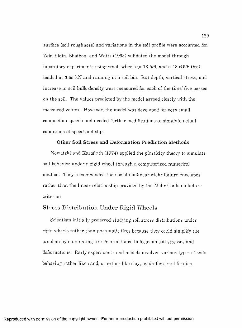
129
surface (soil roughness) and variations in the soil profile were accounted for.
Zein Eldin, Shaibon, and Watts (1993) validated the model through
laboratory experiments using small wheels (a 13-5/6, and a 13-6.5/6 tire)
loaded a t 3.65 kN and running in a soil bin. Rut depth, vertical stress, and
increase in soil bulk density were measured for each of the tires’ five passes
on the soil. The values predicted by the model agreed closely with the
measured values. However, the model was developed for very small
compaction speeds and needed further modifications to simulate actual
conditions of speed and slip.
O th e r Soil S t re s s a n d D e fo rm a t io n P r e d ic t io n M e th o d s
Nowatzki and Karafiath (1974) applied the plasticity theory to simulate
soil behavior under a rigid wheel through a computerized numerical
method. They recommended the use of nonlinear Mohr failure envelopes
ra the r than the linear relationship provided by the Mohr-Coulomb failure
criterion.
S t r e s s D i s t r i b u t i o n U n d e r R i g i d W h e e l s
Scientists initially prefeired studying soil stress distributions under
rigid wheels ra the r than pneumatic tires because they could simplify the
problem by eliminating tire deformations, to focus on soil stresses and
deformations. Early experiments and models involved various types of soils
behaving ra the r like sand, or ra ther like clay, again for simplification
R eproduced with perm ission of the copyright owner. Further reproduction prohibited without perm ission.

1 3 0
(Vincent, 1961; Wong and Reece, 1966; Dagan and Tulin, 1969; Chung
and Lee, 1975).
Block et al. (1990a) tested various stress prediction methods against
actual measurements obtained with a rigid wheel equiped with 5 contact-
stress transducers, and a stress-state transducer buried 0.30 m below the
soil surface. The prediction methods were, on one hand, the finite element
method combined with other models attempting to describe the nonlinear
behavior of agricultural soil, and the Boussinesq-Cerruti general equation
modified with a Frohlich concentration factor of 6. Overall, the results
given by the finite element method were in satisfactory agreement with
experimental values while the Boussinesq-Cerruti-Frohlich method
underpredicted the soil stress level obseiwed by the underground stress-
state transducer.
Block et al. (1990b) developed a three-dimensional computer-graphic
display model of a rigid wheel to visualize soil stress levels recorded by
underground stress state transducers and tire-soil interface stresses
recorded by a specially equipped rubber-coated rigid wheel (1.372 m
diameter and 0.305 m width). This tool was developed to help study both
soil stresses and tire-soil contact stresses through computer animation of
wheel motion.
R eproduced with perm ission of the copyright owner. Further reproduction prohibited without perm ission.

1 3 1
S tress D istr ib u tio n U nder T ires
If the load distribution (or pressure distribution) a t a tire-soil interface
were known, stress distribution could be computed by the equations given
above. Bekker (1956) emphasized on the necessity to account for both
vertical and horizontal loads:
When vehicles act upon the soil, they do not exercise vertical loads only. Horizontal loads H have to be exercised not only in order to pull an agricultural implement or trailer, but also in order to keep a vehicle moving.
Koolen and Kuipers (1983), and Plouffe et al. (1991) omitted horizontal
loads in their computations, which yielded unsatisfactory results when
comparing to experimental measurements. Johnson and Burt (1990)
accounted for tangential loads and obtained better results.
Most models did not account for soil deformations under the load and
assumed a rigid loading area, while tires were actually flexible, thus
producing a three dimensional contact area (Soehne, 1958; Plouffe et al.,
1991). Some models also assumed a uniform load distribution (Plouffe et
al., 1991), while measurements proved this assumption to be very different
from reality (Wood, Burt, and Johnson 1991). Actually, interface pressure
distribution was unknown, and assumptions had to be made concerning the
surface load distribution to then compute stresses in the soil. Several load
distribution functions have been used, other than tha t of uniform loading
(Plouffe et al., 1991).
R eproduced with perm ission of the copyright owner. Further reproduction prohibited without perm ission.

1 3 2
Load D istr ib u tion M odels
Soehne (1958) made the following observations:
The tire track on any soil will become deeper with increasing porosity moisture content. The deeper the tire track, the larger the contact area. The average surface pressure decreases accordingly.
An approximately equal pressure over the entire contact area can be assumed when large-volume tires without lugs are in contact with hard dry soil. This is not true for plastic and soft soils. In the contact area, the pressure depends upon the specific depth of the track. If there is plastic flow to the side of the contact area on a moist soil and soil compaction under the tire, then the pressure decreases toward the outside of the contact area and the pressure is more concentrated towards the center of the load.
- S oeh n e lo a d d istr ib u tion m odel:
Soehne (1958) used load distributions developed for a flat circular area
to find the size of the contact area between the tire and the soil. However,
only vertical loads were considered. Calling A the contact area, then:
f p , oW (163)
where:
W = total load, and
p . = contact pressure at any point of the contact surface.
The pressure distribution on a circular contact area was given by:
where:
Rc = radius of the circular area.
\ f p ' " '
\ ^ c j /
(164)
R eproduced with perm ission of the copyright owner. Further reproduction prohibited without perm ission.

133
Pc = respective distance of the relation point from the center of the
circle area, and
m = exponent for parabolic pressure distribution,
m = 16 for a dense, hard dry, cohesive soil which was only elastically
deformable (parabola of the 16“' degree), which gave = 1.125 (p mcun:
m = 4 for a sandy clay soil, fairly moist, relatively dense (parabola of the
fourth degree), thus (Pc)^» = 1-5 (pjmeun:
m = 2 for a plastic flowing wet soil (quadratic parabola), thus
^P c^ m ax ^ ^ P c ^ n ïe a n '
- J o h n so n and B urt load d istr ib u tion model:
Jolinson and Burt (1990) used the following equation for the distribution
of the normal pressure:
Pi pc + ipe - pc)/ \ y X
max / Vw ith
and
pc
2Ê > 0pc
( m + 1 )" V
m m + p epc)
where:
pc = normal pressure at the center of the footprint.
(163)
(166)
(167)
R eproduced with perm ission of the copyright owner. Further reproduction prohibited without perm ission.

1 3 4
pe = normal pressure a t the sides of the footprint,
m = power for parabolic pressure distribution,
P’mcan = avoruge normal pressure over the footprint,
X , y = X and y coordinates of the i'*’ point within the footprint,
x„,ax> Ymax = ono-half of footprint length and width a t the x-y
coordinates, respectively, and
p ’i = normal pressure over the i"' elementary square area A, (2.5 cm x
2.5 cm).
Three different load distributions were compared:
1. uniform load distribution (type I),
2. m = 2 and pe/pc = 0.5 (type II), and
3. m = 2 and pe/pc = 2 (type III).
For each elementary square area A , the elementary normal load was
lüj = p ' Aj ( 1 6 8 )Therefore, the tire dynamic load was
= 2] w; (169)i
The horizontal, or shear component H, of the load, aligned in the
direction of travel, was either supposed to be uniformly distributed, or
modeled as:
_ h
Hi = Aj (c + p I tan((j))) U - e ^(170)
R eproduced with perm ission of the copyright owner. Further reproduction prohibited without perm ission.

1 3 5
where:
= horizontal component on elementary area A,,
c = soil cohesion coefficient,
(J) = soil in ternal friction angle,
jj = shear displacement a t Aj, assumed to vary linearly from zero at
the leading front edge of the tire footprint, to a maximum value equal
to the product of the footprint length and travel reduction a t the
trailing rea r edge of the footprint, and
kj = shear displacement coefficient.
Gross traction GT was expressed as
= ( 1 7 1 )i
Note th a t the forces were assumed to act on a plane surface (equivalent flat
footprint). Johnson and Burt (1990) developed a FORTRAN program to
predict the complete state of stress at any point beneath a tire:
The program transforms the principal stresses for each point load to a stress tensor in a fixed cartesian coordinate sytem, determines the stress state for all the point loads combined, and then determines the principal stresses (g„ o.,, and Gj) and the stress invariants (mean normal stress (Gj + g + g .j)/3, and octahedral shear stress ((g , - g J ' + (g , - G;j)" + (Go - Gj)-)" Y3 ) and their directions.
Sinkage was not given as an output, but corrections for ru t depth were
included in the program. Therefore, a simple modification of the program
could provide sinkage information.
Special stress sensors were developed by the NSDL to measure soil
stresses under wheels. Way et al. (1993a) used these sensors to study the
R eproduced with perm ission of the copyright owner. Further reproduction prohibited without perm ission.

1 3 6
effect of tire lug height on subsurface soil stresses, for example. Tire lug
height was found to have no significant effect on soil stresses when the
sensors were buried below 0.16 m or more of soil in the NSDL indoor soil
bins.
I n t e g r a t e d T o o ls a n d C o m b in e d M e th o d s
Raper et al. (1991) combined the tools developed by the NSDL and
Auburn University, Auburn, Alabama, to predict soil compaction and help
farmers avoid soil compaction. Four areas were included in this overall
effort: m easurem ent of soil-tire interface stresses, measurem ent of soil
stresses, development of constitutive stress-strain i-elationships for
agricultural soils, and development of analytical and finite element soil
compaction models. Raper et al. were thus proposing a complete set of tools
to study soil phenomena from a traction point of view.
Guo and Schuler (1992) combined the finite difference method and the
finite element method in a two dimensional soil and wheel interaction
model. The finite difference method was used in conjunction with the Mohr-
Coulomb failure criterion to determine, under critical failure conditions, the
soil failure patterns induced by the tire load, thus predicting the tire-soil
interface stress state. The shape of the tire-soil interface in the plane of
symmetry was assumed to consist of two exponential portions linked by a
s tra ight line. The finite element method was then used to compute stresses
within the soil. The finite element model provided graphical illustrations of
R eproduced with perm ission of the copyright owner. Further reproduction prohibited without perm ission.

1 3 7
stress contours in the soil. This method was then validated by a series of
laboratory experiments.
Soil-W heel C ontact S tresse s
Using a simple technique developed earlier by Burt and Schafer (1972)
to m easure tangential stresses a t the interface between soil and a split rigid
wheel while recording wheel torque, Bailey and Burt (1976) compared the
resu ltan t forces computed from measured stresses to the forces required by
a torque balance. In all cases, the resu ltan t tangential force was sligthly
less than the ratio of torque to wheel radius (T/r). Although this
discrepancy was recognized to cause only minute errors in wheels mechanics
calculations, it was pointed out as a source of questioning on a mechanical
analysis standpoint. Numerous soil-wheel contact stress m easurements
were then made a t NSDL to better understand how these stresses develop
and how they affect traction (Wood and Burt, 1987a and 1987b; Burt,
Wood, and Bailey 1989).
Burt, Wood, and Bailey (1990, 1992) made comparisons between several
methods of determining the contact pressure between a tire and the soil.
Their results showed tha t on compacted soils, the peak pressures measured
a t the soil-tire interface were much greater than mean pressures
determined from measurements and greater than pressures calculated by
dividing the djmamic load by the contact area. On uncompacted soil, peak
R eproduced with perm ission of the copyright owner. Further reproduction prohibited without perm ission.

138
pressures are almost equal to the inflation pressure. Other interesting
conclusions were made:
1. The average contact pressure on a rigid surface was fairly close to the inflation pressure.2. The average contact pressure on a rigid surface was almost constant across a wide range of dynamic loads, indicating th a t the contact area between the tire and a rigid surface increases almost directly in proportion to increases in dynamic load.3. Tire dynamic load divided by the dynamically measured tire contact area on soil was almost constant regardless of soil type or condition and equalled about half of the inflation pressure.4. The inflation pressure was not greatly exceeded by any of the average pressures investigated.5. Since the peak resultant pressure was the pressure of highest observed magnitude, it likely will determine the magnitude of the soil compaction which will result from the passage of the tire.
Block, Burt, and Johnson (1989) developed a three-dimensional
computer-graphics program to display stress and deformation
measurements obtained from a tire instrumented with surface stress
sensors, as it traveled on soil. This permitted a quick and detailed
visualization of stress levels and deformations of a tire lug. Conclusions
made earlier based on the same data were rapidly confirmed, and further
observations were made that enhanced the analysis of the phenomena
occuring a t the tire-soil interface. In particular, tangential-to-normal stress
ratios greater than 1.0 were observed. Block, Burt and Johnson suggested
tha t an adhesion phenomenon occured at the tire-soil interface. Also,
differences in stress levels and deformations along the lug were pointed out.
Wood, Burt, and Johnson (1991) studied how thrust (gross traction) was
distributed across the width of an 18.4R38 tire a t four different levels of
R eproduced with perm ission of the copyright owner. Further reproduction prohibited without perm ission.

139
dynamic load, both in loose and compacted soil conditions for the two types
of soils located in the NSDL soil bins (Norfolk sandy loam and Decatur clay
loam). Slip was set a t 18.5% to represent a powered wheel operating on
tilled soil, and forward velocity was held constant at 0.15 m/s. Five
locations were used for the tire-soil contact sensors: tire centerline, lug
center, lug edge, and two undertread locations (between lugs). Thrust
appeared to be developed more uniformly across the lug face in loose soil
conditions than in compacted soil because loose soil deformed to the tire
shape. No significant differences in thrust across the lug of the tire wore
observed for the tire operating at full rated load in the loose Decatur clay
loam soil. Thrust increased with dynamic load a t the extremities of the lug
(tire center and lug edge). On compacted soil, lug center th rus t was not
significantly affected by dymamic load, and was significantly less than tire
centerline thrust. In loose soil, lug center thrust was equal to tire
centerline thrust. Thrust contributions beyond the bottom center point of
contact at the tire center and lug edge areas were predominant when
operating at full rated load on compacted soil. No significant difference in
th rus t generation was obseiwed at the two undertread positions on any of
the 4 soil conditions, but the contribution of the undertread to the overall
th rus t was higher in the loose soil than in the compacted soil.
Way et al. (1993b) showed th a t tire-soil interface pressures on the lug
face increased with tire lug height and soil firmness, while they decreased
R eproduced with perm ission of the copyright owner. Further reproduction prohibited without perm ission.

1 4 0
on the undertread (between the lugs). This was observed with tlxree
instrum ented 18.4R38 R-1 tires with lug heights of 31%, 55%, and 100% of
the new tire lug height, respectively, tested in the NSDL indoor soil bins.
Effects of inflation pressure and dynamic load on soil deformation and tire-
soil interface stresses was investigated by Raper et al. (1993) with another
similarly instrum ented tire. Stress levels increased, particularly near the
center of the tire footprint, as inflation pressure or load increased. Raper et
al. also presented a method to determine the total contact area and the total
contact length by analysing the stress measurements.
Okello (1992) presented a model for the shape of the tire-soil interface
under small sinkage conditions. The portion of the interface ahead, in the
direction of travel, of the line of application of the wheel load was
considered as a spiral curve, and the portion following the line of
application of the load was assumed flat. This model was combined with
the Bekker pressure-sinkage and shear stress-strain relationships to
compute the forces generated at each point of the interface. These forces
were then integrated to determine the resultant force at the interface. An
interactive process was used to compute the sinkage and slip values
satisfying the force equilibrium condition. Traction performace could then
be predicted (gross traction, motion resistance, net traction and tractive
efficiency). The model was then tested against empirical results
represented by the Gee-Clough traction model. Theoretical prediction
R eproduced with perm ission of the copyright owner. Further reproduction prohibited without perm ission.

1 4 1
agreed very well with empirical results for slip values of 0 to 25%, but
diverged for higher values. Okello suggested th a t a more acurate
assessm ent of soil parameters as determined by Bekker’s plate sinkage
method would further improve the results.
Other researchers have measured soil-wheel interface stresses (Krick,
1969) and models have been proposed (Wong, 1984) but found limited use,
due probably to their complexity (Yong and Foda, 1990) or their limitation
to rigid wheels (Wong and Reece, 1967).
T ra ctio n M odel B ased on Soil-W heel C ontact S tresses
A review of the mechanics of a deformable wheel on soft soil was
presented by Wulfsohn and Upadhyaya (1991). The equations for net
traction NT and dynamic load W were.
JVT = j ^ (T(i[r) cos<I> - sin0) (172)
and.
17 = (t(i|/) sinO + o„(t};) cos$) cL4 . (173)
where;
t = shear stress at soil-tire contact surface,
= normal stress at soil-tire contact surface,
(I> - angle between surface normal and vertical at any point on
contact surface.
R eproduced with perm ission of the copyright owner. Further reproduction prohibited without perm ission.

1 4 2
Y = vertical angle from tire axle to a point on the contact surface, and
Ag = soil-tire contact surface.
F ig u r e 19 shows the wheel model used by Wulfsohn and Upadhyaya.
An equation was given to estimate the mean normal stress acting over
the contact area between a tire and a rigid surface:
where:
W = vertical load,
A = contact area, and
p,„ = mean contact pressure.
(174)
d ir e c t io n o f tra v e l
NT
SOIL SURFACE
F igure 19. Force equ ilibrium of a pow ered w h eel (W ulfsohn and U padhyaya, 1991).
R eproduced with perm ission of the copyright owner. Further reproduction prohibited without perm ission.

1 4 3
The mean contact pressure on a rigid surface was calculated as;
Pm = 4 P ^ P c (175)where:
p = tire inflation pressure,
Pc = average pressure transmitted by the tire carcass when p = 0, and
q = a constant of tire stiffness having a value between 0.6 (high
pressure tires) and 1.0 (low pressure tires).
The stress distribution over the contact area was estimated with the
Bernstein pressure-sinkage model:
and
G. = (176)
b (177)where:
b = tire width (m),
z - sinkage depth (m),
k^ = soil stiffness constant (Pa),
lÿ, k and n = coefficients obtained from sinkage plate tests.
The shear stress was assumed to be expressed by the Micklethwaite
equation:
(c + o„ tan((j))) \ l - e
R eproduced with perm ission of the copyright owner. Further reproduction prohibited without perm ission.

1 4 4
where:
j = shear deformation,
kj = soil shear displacement coefficient,
c = soil cohesion, and
(?) = soil in ternal angle of friction.
All these soil param eters were obtained from grouser plate tests made in
situ. Wulfsohn and Upadhyaya developed a model of tire-soil interactions
based on m easurements of the three-dimensional dynamic contact area
between a tire and the soil. They observed tha t the shape and size of the
contact area depended on the soil condition (firm versus tilled), the dynamic
load, the tire inflation pressure, and wheel slip.
Other models have been presented which used soil-tire interface stresses
(Schuring, 1964; Fujimoto, 1977). The work by Schuring was based on
previous work by Bekker (1956 and 1960), while Fujimoto referred to
equations presented by Wong and Reece (1967). The lack of expeiimental
data on soil-tire interface stresses, due mainly to the difficulty to measure
these, prevented comparison between model predictions and actual values.
E x p e r i m e n t a l T r a c t i o n R e s u l t s
B urt and Bailey (1975) and Bailey, Burt, and Taylor (1976) recorded the
gross traction versus dynamic load curves of rigid wheels under various soil
and wheel conditions: Smooth steel wheel, grousered steel wheels vath
various grouser constructions, rubber coated steel wheel, loose or compacted
R eproduced with perm ission of the copyright owner. Further reproduction prohibited without perm ission.
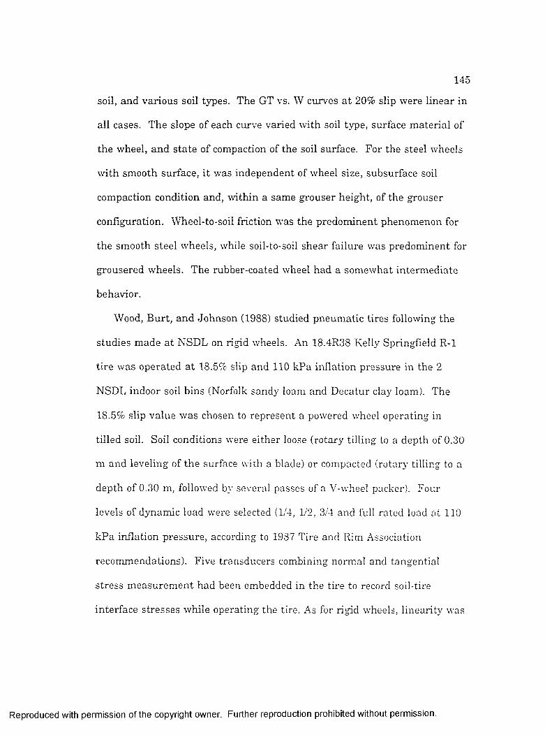
1 4 5
soil, and various soil types. The GT vs. W curves a t 20% slip were linear in
all cases. The slope of each curve varied with soil type, surface material of
the wheel, and state of compaction of the soil surface. For the steel wheels
with smooth surface, it was independent of wheel size, subsurface soil
compaction condition and, within a same grouser height, of the grouser
configuration. Wheel-to-soil friction was the prédominent phenomenon for
the smooth steel wheels, while soil-to-soil shear failure was prédominent for
grousered wheels. The rubber-coated wheel had a somewhat intermediate
behavior.
Wood, Burt, and Johnson (1988) studied pneumatic tires following the
studies made a t NSDL on rigid wheels. An 18.4R38 Kelly Springfield R-1
tire was operated a t 18.5% slip and 110 kPa inflation pressure in the 2
NSDL indoor soil bins (Norfolk sandy loam and Decatur clay loam). The
18.5% slip value was chosen to represent a powered wheel operating in
tilled soil. Soil conditions were either loose (rotary tilling to a depth of 0.30
m and leveling of the surface with a blade) or compacted (rotary tilling to a
depth of 0.30 m, followed by several passes of a V-wheel packer). Four
levels of dynamic load were selected (1/4, 1/2, 3/4 and full rated load at 110
kPa inflation pressure, according to 1987 Tire and Rim Association
recommendations). Five transducers combining normal and tangential
stress m easurem ent had been embedded in the tire to record soil-tire
interface stresses while operating the tire. As for rigid wheels, linearity was
R eproduced with perm ission of the copyright owner. Further reproduction prohibited without perm ission.

1 4 6
observed for the gross traction versus dynamic load curves. Intercepts were
not significantly different from zero. This agreed with the fact th a t a tire
should produce no gross traction under zero load (GT = 0 when W = 0). The
slopes of the curves depended on the soil types, and were higher for Decatur
clay loam (27% sand, 43% silt and 30% clay) than for Norfolk sandy loam
(72% sand, 17% silt and 11% clay). Compaction level did not seem to affect
slope values within a same soil type. This was explained by the fact tha t
the top layer of the soil was similar with respect to cone index and bulk
density in both loose and compacted condition, and previous work had
shown th a t subsuface compaction did not influence the GT vs. W
relationship. The linear relationship between gross traction and dynamic
load for the Kelly Springfield 18.4R38 R-1 tire a t 18.5% slip and 110 kPa
inflation pressure, in Norfolk sandy loam and for both compacted and loose
conditions, was
G T = -0.066 + 0.628 W (179)with an R“ value of 0.960. A rubber-coated rigid wheel was operated under
the same conditions and linear relationships between GT and W also found.
Another linear model was developed to relate the slopes of the GT vs. W
curves obtained with the rigid wheel to those of the pneumatic tire. This
indicated th a t a rigid wheel could be used to predict the gross traction
developed by a radial tire.
R eproduced with perm ission of the copyright owner. Further reproduction prohibited without perm ission.

1 4 7
Upadhyaya (1988) was able to difierentiate, according to tractive
performance, five 18.4-38 tires presenting various tread designs. Tread
design studies had been somewhat neglected prior to th a t because this
variable was not ranked among the most significant ones with respect to
tractive performance.
R eproduced with perm ission of the copyright owner. Further reproduction prohibited without perm ission.

EXPERIMENTAL SETUP AND EXPERIMENT
DESCRIPTION
Three types of experiments were performed; m easurement of static
properties of tires in the vertical direction (deflection vs. load, and stiffness
vs. inflation pressure); measurement of dynamic properties of tires in the
vertical direction (deflection and load vs. time and inflation pressure,
stiffness and damping coefficient vs. inflation pressure); and measurement
of tractive performance on soil. The first two sets of tests were done at
LSU, in the Biological and Agricultural Engineering department laboratory,
with a machine specially designed and built for this project. The last part
was done a t the United States Department of Agriculture, Agricultural
Research Service (USDA-ARS) National Soil Dynamics Laboratory (NSDL)
in Auburn, Alabama, with cooperation of their personnel.
Static Measurements
A p p a r a t u s f o r S t a t i c E x p e r i m e n t s
The tire-loading machine built at LSU was designed using AutoCAD
(Autodesk, Sausalito, California) computer-aided-design software to
facilitate future modifications, parts reuse, and possible construction of a
similar machine. The machine consisted of several subassemblies: frame,
axle, wheel attachment, loading system, oscillatory mechanism,
148
R eproduced with perm ission of the copyright owner. Further reproduction prohibited without perm ission.

1 4 9
displacement transducer, tire load scale, and data logging system (F ig u res
20 a n d 21).
The L-shaped frame was made of 12.7 mm-thick steel plate and 152.4
mm-I beams welded at the bottom to 101.6 mm-I beams, which provided
additionnai rigidity and helped support the load scale. Two guides were
bolted inside the frame to hold the oscillatory mechanism horizontally.
Four tracks were welded to the vertical part of the frame to guide the axle.
Other features included lifting hooks, ears to a ttach the compression
system, and an eye-bolt to adjust the oscillatory mechanism vertically. The
axle housing was guided on the frame by 8 rollers, moving only in the
vertical direction. The 4 rollers located on the front side of the machine
were cone-shaped for lateral guidance. The 4 back rollers were attached
with eccentric bolts to compensate for clearances and to allow for a preload
to make the frame-to-axle connection stiffer. A transverse shaft on top of
the axle housing received both the top part of the eccentric mechanism rod
and the quick-attach clamp of the hydraulic loading system. The axle shaft
was a used tractor rear axle and was mounted on journal bearings to allow
for rotation and thus for measurements a t various tire angular positions.
The wheel a ttachm ent system was designed to allow for various tire
sizes to be tested. The hub remained on the axle shaft; The center plate,
19 mm-thick, was changed to accommodate each rim diameter. A dial was
glued to the back of each center plate and an indicator bolted to the frame
R eproduced with perm ission of the copyright owner. Further reproduction prohibited without perm ission.

1 5 0
TOP V IE W (SC A LE REMOVED)
FRONT V IE W
S ID E V IE W
F igu re 20. CAD d raw ing of th e LSU tire-load in g m achine.
R eproduced with perm ission of the copyright owner. Further reproduction prohibited without perm ission.

1 5 1
F ig u r e 21. G e n e ra l v iew of th e LSU t i re - lo ad in g m ach in e .
to record the angular position of the tire within ±0.1 degree. A maximum of
31 kN compression force could be provided through a double-acting
hydraulic cylinder, 76.2 mm bore by 609.6 mm stroke, pinned to a U-shaped
subframe bolted to the top of the machine frame. Force was transmitted to
the axle through a quick-attach clamp facilitating the discoimection of the
hydraulic cylinder during dynamic tests. Hydraulic pressure came from a
hydraulic hand-pump through a 4-way 3-position directional control valve to
compress or lift the tires. The load scale, located directly under the tire.
R eproduced with perm ission of the copyright owner. Further reproduction prohibited without perm ission.
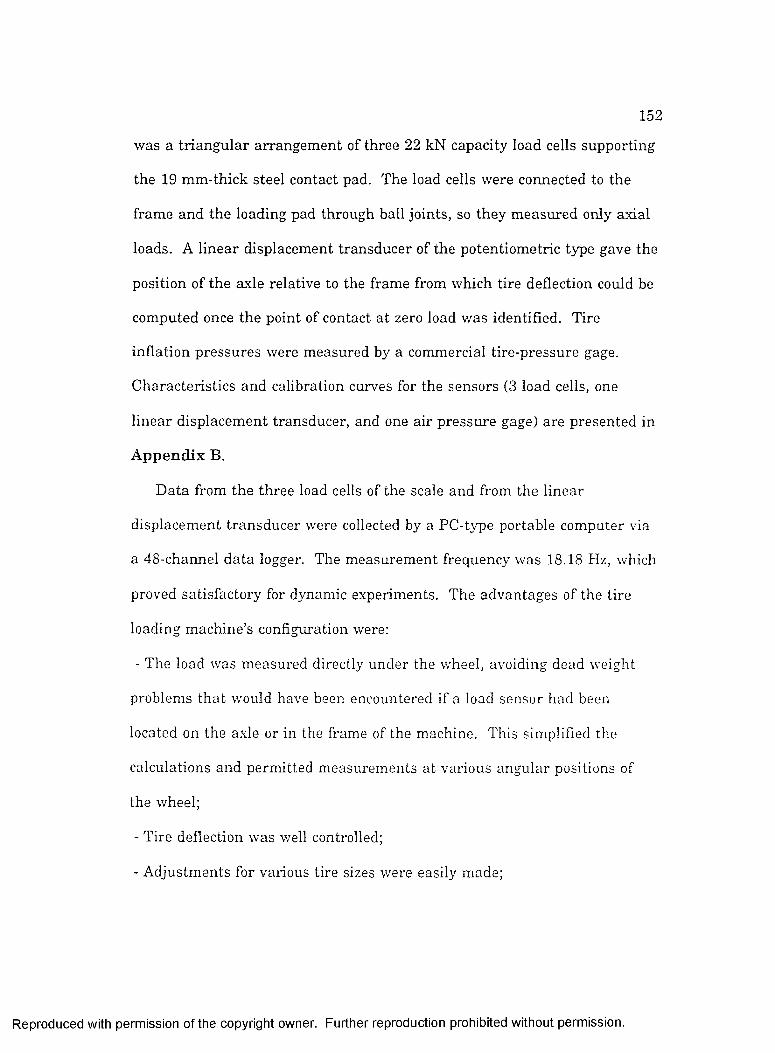
1 5 2
was a tr iangular arrangement of three 22 kN capacity load cells supporting
the 19 mm-thick steel contact pad. The load cells were connected to the
frame and the loading pad through ball joints, so they measured only axial
loads. A linear displacement transducer of the potentiometric type gave the
position of the axle relative to the frame from which tire deflection could be
computed once the point of contact at zero load was identified. Tire
inflation pressures were measured by a commercial tire-pressure gage.
Characteristics and calibration curves for the sensors (3 load cells, one
linear displacement transducer, and one air pressure gage) are presented in
A p p e n d ix B.
Data from the three load cells of the scale and from the linear
displacement transducer were collected by a PC-type portable computer via
a 48-channel data logger. The measurement frequency was 18.18 Hz, which
proved satisfactory for dynamic experiments. The advantages of the tire
loading machine’s configuration were:
- The load was measured directly under the wheel, avoiding dead weight
problems tha t would have been encountered if a load sensor had been
located on the axle or in the frame of the machine. This simplified the
calculations and permitted measurements at various angular positions of
the wheel;
- Tire deflection was well controlled;
- Adjustments for various tire sizes were easily made;
R eproduced with perm ission of the copyright owner. Further reproduction prohibited without perm ission.

1 5 3
- The machine was designed in a modular fashion to facilitate subsequent
modifications and allow measurements under different conditions.
- M easurements of contact area were feasible (some were actually
performed). Contact area and deflection measurements on a soft surface
(soil-filled box) were also contemplated, but height limitations of the
machine precluded them for the larger tires.
Twenty tires with inner tubes were provided by the Pirelli-Armstrong
Tire Company, New Haven, CT. Tires and tubes were delivered in 2
batches to LSU (March 7, 1991, and February 28, 1992). Four commercial
rims were purchased without their a ttachm ent systems. Rim sizes were
selected to match all the tires with a minimum number of rims, following
recommendations of the Tire and Rim Association (1989). Special rings and
lugs were machined, then welded inside the rims to bolt on the circular
plates used as rim centers. A p p e n d ix C contains the data concerning the
tires, inner tubes, and corresponding rims.
S ta tic E xp erim en t D escr ip tion
F ig u r e 22 shows a schematic of the experimental setup used to measure
tire static stiffness. The following steps were taken;
1 - A tire was mounted on the test stand with the appropriate rim;
2 - Inflation pressure was set to its recommended maximum;
3 - The tire was lowered until it came in contact with the contact pad;
4 - Recording of tire load and axle position was started;
R eproduced with perm ission of the copyright owner. Further reproduction prohibited without perm ission.

1 5 4
HYDRAULIC CYLINDER
TIRE
AXLE LOADCELL
FRAME
F ig u r e 22, S c h e m a t ic o f a s ta t ic t i r e - lo a d in g e x p e r im e n t .
5 - The load was increased until it reached the maximum load recommended
by the Tire and Rim Association (1989) and ASAE Standard 8430 (1989b)
for the set inflation pressure;
6 - The load was slowly reduced to zero, ie- until the tire barely touched the
contact pad (a sheet of paper placed between the tire and the contact pad
became loose);
7 - Steps 5 through 6 were repeated to reduce measurement errors and to
detect any hysteresis (preliminary tests showed tha t going through the
loading-unloading cycle more than twice did not improve the results
significantly);
8 - After recording ended, the tire was lifted off the contact pad;
R eproduced with perm ission of the copyright owner. Further reproduction prohibited without perm ission.

1 5 5
9 - Inflation pressure was set to a lower value and steps 3 to 8 were
repeated. Step 9 was repeated as many times as necessary, with inflation
pressure increments of 13.8 kPa (2 psi on the air pressure gage) to cover the
whole range of recommended tire inflation pressures, plus the lower
pressures of 69, 55 and 41 kPa;
10 - D ata was then transferred to a Lotus 1-2-3 spreadsheet for analysis.
Load cycles were plotted and linear regression analysis provided an
experimental value of static stiffness.
D ata C ollected
Ten tires were used for static tests: 14.9-30 #2, 14.9R30 #3, 16.9-30 #5,
16.9R30 #7, 18.4-30 #9, 15.5-38 #11, 15.5-38 #13, 16.9-38 #15, 18.4-38 #17,
and 18.4R38 #20 (F igure 23). For each test, there were two loading-
unloading cycles. Each record was the average of 10 readings, one every
0.055s. Thus, each data file contained 763 records, representing 7630
observations of load and deflection. The maximum load for each cycle was
approximately equal to the maximum manufacturer-recommended load.
Filenames started with the letter S, for "static", followed by 1 or 2 digits for
the tire number, the letter P, for "pressure", 2 digits for the inflation
pressure expressed in psi, the letter C to avoid confusion, and 1 digit for the
replication. For example, file S3P12C1.PRN contained data for the first
replication of the static test of 14.9R30 tire #3 at 83 kPa (12psi). Of the two
R eproduced with perm ission of the copyright owner. Further reproduction prohibited without perm ission.

1 5 6
F ig u r e 23. T ire sizes u sed in s ta t ic a n d d y n a m ic e x p e r im e n ts .
replications done for each test, the one giving the highest R' value for linear
regression of deflection versus load was kept. Each static deflection data
file contained:
* On the top row,
- The date and hour, as given by the computer clock;
- The name of the setup file used for the test;
- The number of channels used on the data logger;
- The sampling rate, in minutes.
* On the second row, the numbers of the channels used, as identified on the
data logger.
R eproduced with perm ission of the copyright owner. Further reproduction prohibited without perm ission.
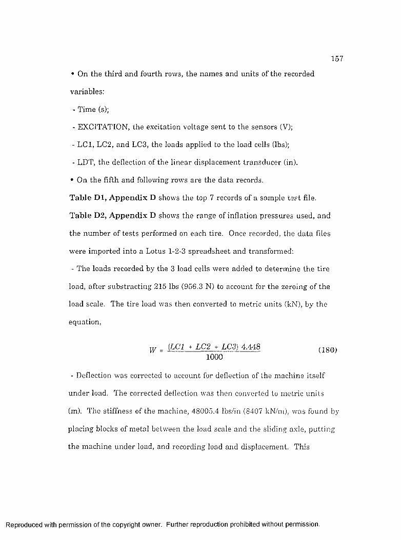
1 5 7
• On the third and fourth rows, the names and units of the recorded
variables:
- Time (s);
- EXCITATION, the excitation voltage sent to the sensors (V);
- LCl, LC2, and LC3, the loads applied to the load cells (lbs);
- LDT, the deflection of the linear displacement transducer (in).
• On the fifth and following rows are the data records.
T ab le D l , A p p e n d ix D shows the top 7 records of a sample test file.
T ab le D2, A p p e n d ix D shows the range of inflation pressures used, and
the number of tests performed on each tire. Once recorded, the data files
were imported into a Lotus 1-2-3 spreadsheet and transformed:
- The loads recorded by the 3 load cells were added to determine the tire
load, after substracting 215 lbs (956.3 N) to account for the zeroing of the
load scale. The tire load was then converted to metric units (kN), by the
equation,
jpr _ (LCl + LC2 + LC3) 4.448 (180)1000
- Deflection was corrected to account for deflection of the machine itself
under load. The corrected deflection was then converted to metric units
(m). The stiffness of the machine, 48005.4 lbs/in (8407 kN/m), was found by
placing blocks of metal between the load scale and the sliding axle, putting
the machine under load, and recording load and displacement. This
R eproduced with perm ission of the copyright owner. Further reproduction prohibited without perm ission.

1 5 8
operation was repeated for various block heights to account for the effect of
axle height, and an average value of machine overall stiffness was
computed. The conversion equation for deflection was,
à = I lD T - 1- ^ ^ ^ ~ n 0.0254I I 48005.4
(181)
- The origin of the load-deflection curve was identified by searching for the
data point where both the deflection and the load were a t a m inim um after
the first peak load had been reached during the double loading-unloading
cycle. This reduced potential error due the eventual settling tim e required
by the data-logging system. F ig u re 24 shows a typical deflection versus
z0501
Q
o.os
0.07
0.06
0.05
0.04
0.03
0.02
0.01
05 10 15 20
VERTICAL LOAD (kN)
EXPERIMENTAL D.ATA REGRESSION LINE
F igu re 24. D eflection versus load curve, 15.5-38 tire #13 at 138 kPa in fla tion pressure.
R eproduced with perm ission of the copyright owner. Further reproduction prohibited without perm ission.

1 5 9
load curve obtained during a static experiment. The load-deflection curves
showed hysteresis, which was attribu ted to the tires because the deflection
of the m achine was accounted for during da ta trea tm ent. This hysteresis
was possibly due to visco-elastic, ra th e r than purely elastic, behavior of the
tire despite the low loading ra te used.
T ests to E v a lu a te M easurem ent E rror
A series of tests was done on the 15.5-38 tire #13 to evaluate
m easurem ent errors under static conditions. This tire was chosen because
it showed some of the largest variations among sim ilar m easurem ents, and
the lowest value for linear regression between vertical stiffness and
inflation pressure. The tests were of 4 types: instrum entation settlem ent
and drift, variations among identical tests, variations w ithin one tire lug-
pitch, and variations around the circumference.
I n s t ru m e n ta t io n S e tt le m e n t a n d D rif t
F irst, the data-logger was run for 7 m inutes, the usual duration of a
load-deflection test, with the tire left in the same position, with no load
applied, to observe any settlem ent or drift effect due to the data gathering
system (load cells, linear displacement transducer, da talogger and portable
computer). Load and displacement were recorded as shown on F ig u re 25.
Amplitude of the variations was computed. Load showed a sharp fall
during the first 20 seconds, corresponding to a settling time for the system
R eproduced with perm ission of the copyright owner. Further reproduction prohibited without perm ission.

1 6 0
250 0.3
0.25200
0.2
!50
0.15
J 100
0.05
0 100 300 •400 500200
E
HZOJ:sU3CJ<zc-i2a
TLM E (s)
L O A D (N ) D IS P L A C E M E N T (m m )
F igu re 25. S ettlem en t and drift o f the data-logging system in sta tic con d ition s.
comprising the load cells, the data-logger and the computer. Readings
rem ained ra th e r stable afterwards. Amplitude of the load variations was
217 N for the whole test duration, but only approximately 15 N after the
first 20 seconds. Because most of the drop in the load reading occured
before 10 seconds, the records corresponding to the first 10 seconds of all
subsequent tests were ignored during calculations. Thus, the am plitude of
the variations after the first 10 seconds was 50 N. The lowest value of
recommended maximum load for the tires tested was 9163 N (14.9-30 tire at
41 kPa inflation pressure with no extra load). Therefore, the maximum
R eproduced with perm ission of the copyright owner. Further reproduction prohibited without perm ission.

1 6 1
relative error due to initial settlem ent for the tires tested was 50 N / 9163
N = 0.5%. Ignoring the records for the first 20 seconds gave a 15/9163 =
0.16% error.
Displacement m easurem ents seemed much more erratic and had an
am plitude of 0.254 mm, which was compared to the deflection expected
under the maxim um recommended load, computed as:
= I - r, ( 182)
5„ted for the 15.5-38 tire was equal to 52.07 mm. Therefore, the relative
error due to drift of the deflection m easuring system (linear displacement
transducer, data-logger and computer) was 0.254 mm / 52.07 mm = 0.5%.
Ignoring the first 10 seconds (or the first 20 records) appeared sufficient to
reduce the effect of initial instrum entation settlem ent.
V a r ia tio n s A m ong Id e n tic a l T ests
Four sets (one a t 138 kPa, one at 110 kPa, one at 83 kPa and one a t 55
kPa inflation pressure) of 10 load-deflection tests each, all for the same
angular position of the tire, were made. The purpose of these sets was to
evaluate errors due to operator and instrum entation combined. Inflation
pressure was modified only after 10 m easurem ents had been made in the
same conditions (inflation pressure and angular position). F ig u re 26 shows
the stiffness values obtained for each level of inflation pressure. Inflation
pressure levels were evenly spaced, one every 27.6 kPa (4 psi) s tarting from
R eproduced with perm ission of the copyright owner. Further reproduction prohibited without perm ission.

162
55 kPa and up, to cover the operating range of inflation pressures
recommended by the m anufacturer (83 to 138 kPa) and pressures below
th a t range, as well.
400
300
B200
100
— i I i r
Y Y Y V Y V Y i
3 4 5 6 7
MEASUREMENT NUMBER
138 kPa 110 kPa 83 kPa o 55 kPa
10
F igure 26. V aria tion s am ong sim ilar stiffn ess m easu rem ents for 4 lev e ls o f in fla tion p ressu re (15.5-38 tire #13).
V a ria tio n s W itliin O ne T ire L u g -P itc li
Four sets of tests, one set a t 138 kPa inflation pressure, one a t 110, one
a t 83 and one a t 55, of 11 tests each were made, each set equally spaced
along one tire pitch length. The purpose of these sets of tests was to
evaluate variations of stiffness m easurem ents along one pitch length. The
R eproduced with perm ission of the copyright owner. Further reproduction prohibited without perm ission.

1 6 3
tire had 26 a lternating short-bar, long-bar lugs on each side, or 13 pitch-
lengths along its circumference, an angle of 27.692“ per pitch. Tire angular
position could be set w ithin ±0.1° on the machine. Inflation pressure was
modified only after all the m easurem ents for the sam e inflation pressure
level had been made. F ig u re 27 shows the variations of w ithin one
pitch length for the 4 levels of inflation pressure.
400
300
Z200
â 9
100
jg______ _ 1— ----B— 11
0
A------ - "“A' ___A-------- A -----
n- " . ■D - .. O.. ...Q ..... D ' O ..... c 1 - Q
10 15
ANGLE (deg.)20 25 30
138 kPa lOkPa 83 kPa □ 55 kPa
F igu re 27. V ariations o f stiffn ess a lon g one p itch len gth for 4 lev e ls o f in fla tion p ressu re (15.5-38 tire #13).
V a ria tio n s A ro u n d th e T ire C irc u m fe re n c e
Four sets of tests, one a t 138 kPa inflation pressure, one a t 110, one at
83 and one a t 55, of 14 tests each were made, each set equally spaced
R eproduced with perm ission of the copyright owner. Further reproduction prohibited without perm ission.

1 6 4
around the circumference of the tire (every pitch). The purpose of these sets
of tests was to evaluate variations of stiffness m easurem ents from pitch
length to pitch length along the tire circumference, approximately every
27.69°. Inflation pressure was modified only after all the m easurem ents for
the same inflation pressure level had been made. F ig u re 28 shows the
variations of around the circumference of the tire, pitch length by pitch
length, for the 4 levels of inflation pressure.
SI31 '
400
300
200
O
100
0ICO 200
ANGLE (deg.)300 400
138 kPa 110 kPa _ i_ 8 3 k P a □ 55 kPa
F igu re 28. V ariations of stiffness around the circum ference for 4 lev e ls o f in fla tion pressure (15.5-38 tire #13).
F ig u re 29 shows the coefficients of variability CV (standard deviation
divided by average value of the stiffness) for each group of data.
R eproduced with perm ission of the copyright owner. Further reproduction prohibited without perm ission.

1 6 5
□
83 110 138
INFLATION PRESSURE (kPa)
AT FIXED ANGLE E3 AROUND THE CIRCUMFERENCE
WITHIN A PITCH LENGTH
F igure 29. C oefficients o f variab ility for stiffn ess m easurem en ts.
The largest coefficients of variability were observed w ith m easurem ents
within a pitch length, with a CV reaching about 2.6%. These disparities
were probably due to the large geometric variations presented by the lugs.
D isparities around the circumference were a little smaller, with a CV
reaching about 2%, while the CV for m easurem ents at the same angular
position did not exceed 1.8%. The difference between these last two values
was possibly due to non-uniformity of the tire carcass around its
circumference (variations in rubber thickness, off-round, variations of
m aterial properties ...etc). Inflation pressure did not seem to have any
R eproduced with perm ission of the copyright owner. Further reproduction prohibited without perm ission.

1 6 6
definite effect on the observed variations. The m axim um variation
observed, 2.6%, seemed a reasonable indicator of the accuracy of stiffness
m easurem ents.
Dynamic Measurements
A pparatus for D yn am ic E xp erim en ts
A prelim inary assum ption, based on previous research (see C h a p te r 2),
was th a t the behavior of a farm tire in the vertical direction could be
satisfactorily represented by a mechanical system consisting of a spring and
a dam per m ounted in parallel (F ig u re 30).
FRAME
AXLE
SPRING DAMPER
'dynLOADCELL
ECCENTRICMECHANISM
F ig u re 30. S p r in g -a n d -d a m p e r m o d e l o f a tire .
Consequently, the reaction support F acting a t the ground-tire contact was
expressed as the sum of the spring and dam per actions:
R eproduced with perm ission of the copyright owner. Further reproduction prohibited without perm ission.
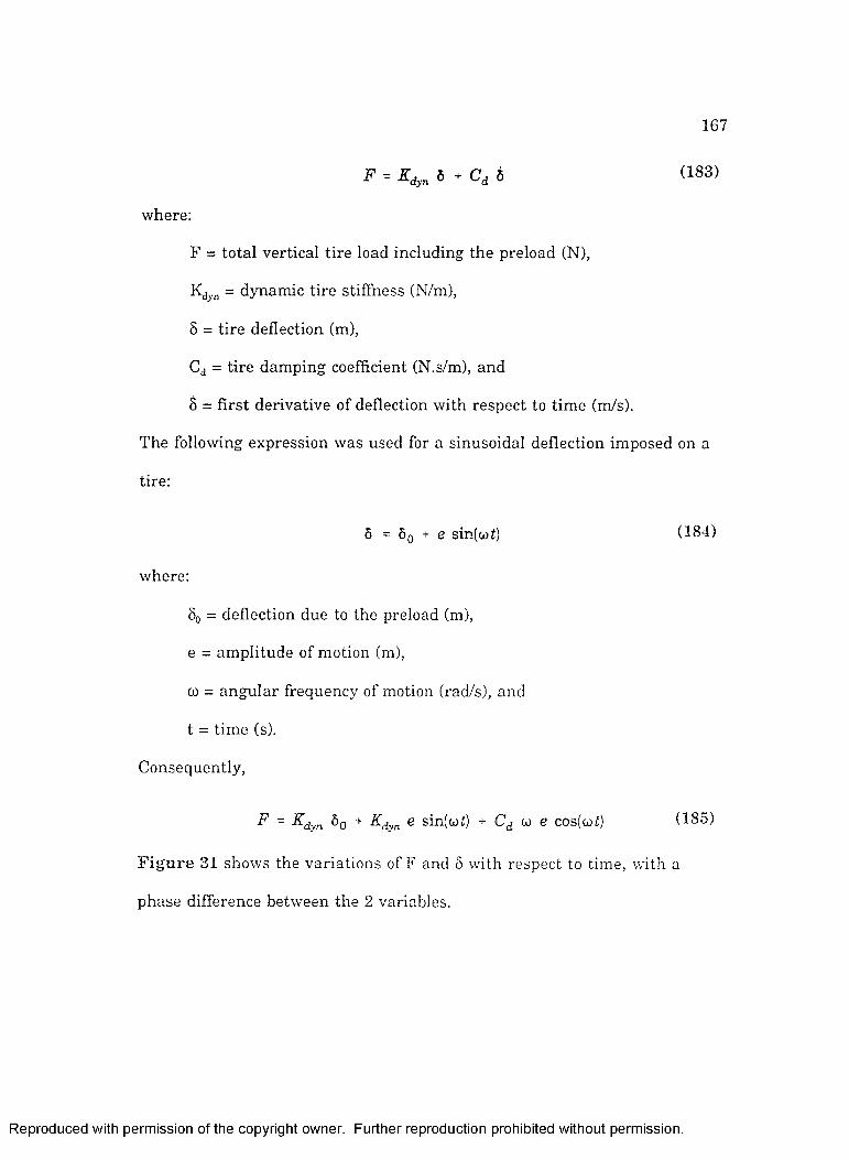
167
f . f ; * Cj & (183)
where:
F = total vertical tire load including the preload (N),
= dynamic tire stiffness (N/m),
5 = tire deflection (m),
Cj = tire dam ping coefficient (N.s/m), and
8 = first derivative of deflection with respect to tim e (m/s).
The following expression was used for a sinusoidal deflection imposed on a
tire:
Ô = Ôq + e sin(cot) (184)
where:
5o = deflection due to the preload (m),
e = am plitude of motion (m),
CO = angular frequency of motion (rad/s), and
t = tim e (s).
Consequently,
F = Ôq + e sin(coi) + Cj w e cos(coi) (185)
F ig u re 31 shows the variations of F and 6 with respect to time, with a
phase difference between the 2 variables.
R eproduced with perm ission of the copyright owner. Further reproduction prohibited without perm ission.

168
25
20
15
10
-10
5 -15
10 S
Zo5 £22
LU Clus < z > c
0.5 1 2.51.5 2
TIME (s)
. LOAD DEFLECTION
F ig u re 31. F o rc e a n d d e flec tio n v e rsu s tim e , th e o re t ic a l p a ra lle l s p r in g -a n d -d a m p e r sy stem (Kjy„ = 504.5 kN /m , Cj = 16.8 s kN/m ).
D e te rm in a t io n o f a n d Cj
Rao (1990) stated th a t the energy dissipated by such a spring-and-
dam per system over a motion cycle was equal to the area of the closed loop
obtained when plotting F versus 5.
f F d l ,cycle
(186)
Or, by developing for F and d5,
^ ^ c y c le = / i ^ d y n i ^ O + ^ s i n ( c o t ) ) + Q W G CO s(co t) )
0(Ôq + e sin(cot)) dt
(187)
R eproduced with perm ission of the copyright owner. Further reproduction prohibited without perm ission.

1 6 9
Solving yields,
The energy dissipated over a motion cycle could be computed directly from
the data and Cj obtained from this equation after computing the area
enclosed in one load vs. deflection loop, such as the one shown in F ig u re
32. The dynamic stiffness was determined from the maximum and
m inim um values of the deflection, which both correspond to a zero velocity.
Assuming a constant dynamic stiffness for the deflection range,
F - F ,K . = - 2 5 ------------------------------------------ (189)Ô - Ô •^max mm
However, the duration of a cycle depended on the eccentiic angular velocity
CO, which varied independently of the data sampling frequency. Therefore, a
motion cycle did not necessarily correspond to a round num ber of data
sam pling periods. The actual shape of the load-versus-deflection loops and
the approxim ations th a t had to be made proved too large for the results to
be accurate enough (F ig u re 33), especially when low values of Cj were
encountered (narrow loop). This determ ination method was then rejected,
in favor of another method presented below.
S e c o n d D e te rm in a tio n M eth o d
Another method to determine both stiffness and damping coefficient was
used for comparison, and then selected because of its higher accuracy.
Deflection and force had the same frequency but a different phase angle.
R eproduced with perm ission of the copyright owner. Further reproduction prohibited without perm ission.

1 7 0
ZaQ<2ugiUJ
Z
û<O►J
gëeu>
25
20
average load15
10
5-15 -10 ■5 0 5 10 15
DYNAMIC DEFLECTION (mm)
F igure 32. T heoretica l tire dynam ic load versus h arm on ie d eflection cycle (Kjy„ = 504.7 kN/m, Cj = 16.8 s kN/m).
25
20
average load15
10
5-15 -10 -5 0 5
DYNAMIC DEFLECTION (mm)10 15
F igu re 33. A ctual tire dynam ic load versu s harm onic d eflec tio n cycle , 14.9R30 tire #3 at 207 kPa in fla tion pressure.
R eproduced with perm ission of the copyright owner. Further reproduction prohibited without perm ission.

1 7 1
Therefore, the force was w ritten as
F = Ôq + Af sin(w( + <j) ) (190)
where:
Af = am plitude of the force variations (N), and
(j),- = phase angle between force and deflection (rad).
The value of was computed as
A = (191) 2
Equating the two expressions for F (E q u a tio n s [185] a n d [190]) and
isolating the sine component from the cosine part, expressions for Kj and
Cj were obtained:
, A, ,192)dyn
and.
Cj = (193)w e
Once Af, e, co and (}),■ were determ ined directly through data analysis, then
Kjy„ and Cj could be computed. Also, knowing tha t
- 0„;e = m a x “ m i n ( 1 9 4 )
2
Then, the two equations for became sim ilar for small values of ()f, thus
showing th a t the former equation could be used for approximations. When
R eproduced with perm ission of the copyright owner. Further reproduction prohibited without perm ission.

1 7 2
5 and F were recomputed using the and Cj values obtained from
E q u a tio n s [192] a n d [193], an 8% error, relative to the m agnitude of the
sinusoidal p a rt of the m easured values of 5 and F, was obtained for each
test. F ig u re 34 shows the fit obtained between the m easured and
computed values. Rao’s energy method gave a 9% relative error, proving
less satisfactory.
%
% o 0 80 8
TIME (s)
MEASURED LOAD COMPUTED LOAD
..o .. MEASURED DEFLECTION <> COMPUTED DEFLECTION
F igu re 34. M easured and com puted load and d eflection versu s tim e, 14.9R30 tire #3 at 207 kPa in fla tion pressure.
Dynamic experim ents used the same machine as described above, except
th a t the loading system was different. The hydraulic cylinder was
disconnected from the axle. A sinusoidal motion was imposed on the axle
by an oscillatory mechanism made of an eccentric shaft actuated by a
R eproduced with perm ission of the copyright owner. Further reproduction prohibited without perm ission.

1 7 3
hydraulic motor through a chain drive (F ig u re 35). This type of
m echanism did not provide a true harmonic motion because of the
in term ediate rod, bu t it was designed to obtain an approximate motion th a t
was close enough, with respect to location, velocity and acceleration of the
axle.
6^= CJ t
F ig u re 35. G eo m etry o f a n e c c e n tr ic m ech an ism .
From the geometry of the mechanism,
L = e sin(8g) + cos(P^ (195)
where:
e = eccentric length (m),
r^ = rod length (m),
Gg = counterclockwise angle from x-axis to eccentric arm (m),
R eproduced with perm ission of the copyright owner. Further reproduction prohibited without perm ission.

1 7 4
p3 = counterclockwise angle from y-axis to rod (m), and
L = distance from eccentric center of rotation to rod free-end (m).
Also,
Tg sin(pg) = e cos(6g) (196)
Isolating P„,
Pg = Arcsin
Replacing in the equation for L,
/e— cos(0g) (197)
L = e sin(0g) + r, cos Arcsin — cos(8g)/
e
\ I I(198)
Therefore, for known values of 0^„ L could be determined. In particular, if
the eccentric was rotating a t a constant angular velocity co (rad/s) then,
6g = w t (199)
where t was the time (s). The expressions for the first and second
derivatives of L with respect to time were derived to compute the location,
velocity and acceleration of the rod free-end and compare them to those of a
simple sinusoidal motion. A FORTRAN program, called ECC2.F0R
(A ppend ix E), which allowed the rod length to be adjusted for various tire
sizes, was w ritten to perform the computations. The value of 0.0127 m was
chosen for the eccentricity because it was less than the lowest rated
deflection for the group of tires to be tested, while being large enough to be
R eproduced with perm ission of the copyright owner. Further reproduction prohibited without perm ission.

1 7 5
m easured with a ra th e r simple instrum entation. Rod length could be
adjusted according to the bolting pa tte rn of the 2 parts of the rod (F ig tire
36). The possible values for the rod length were 0.74295 m, 0.78105 m,
0.81915 m, and 0.85725 m. The shortest rod length gave the largest
discrepancies w hen compared with true harmonic motion, so this length was
used in sim ulations to compare the motion of the m echanism to the desired
motion. The maximum relative differences for location, velocity and
acceleration were found to be 0.0001086 m, 0.0022722 m/s and 0.095242
m/s^, respectively, for co equal to 200 rad/s. The motion imposed on the tire
axle by the eccentric m echanism was considered sufficiently close to a true
sinusoidal motion. A p p e n d ix E includes a listing of program ECC2.F0R
and significant resu lts for the worst possible conditions with respect to
accuracy of the motion.
The vertical location of the oscillatory mechanism within the m ain
frame, and the rod length were adjusted for the various tire sizes and
desired tire preloads using a screw below the eccentric mechanism. The
speed of the motor was varied to obtain several axle oscillation frequencies.
A tachom eter was mounted a t the end of the hydraulic motor shaft to
provide a direct recording of oscillation frequency. Its output was fed into
the data logger. The inertia effects of moving parts on m easurem ents were
reduced to a m inim um because the axle was directly connected to the frame
a t all tim es through the eccentric mechanism and the tire load was
R eproduced witfi perm ission of tfie copyrigfit owner. Furtfier reproduction profiibited witfiout perm ission.

1 7 6
© ©
-1 =
FRONT VIEWSIDE VIEW
F igu re 36. L ength adjustm ent on th e rod o f the eccen tr ic m echanism
R eproduced with perm ission of the copyright owner. Further reproduction prohibited without perm ission.

1 7 7
m easured directly under the tire. The same sensors used for static
experim ents were used for dynamic m easurem ents. The tachom eter was
connected to the data-logger, and the computer could record values from it.
D yn am ic E xp erim en t D escrip tion
The steps below were followed for the dynamic experiments:
1 - A tire w ith the appropriate rim was mounted on the test stand;
2 - The tire was inflated to its maximum recommended pressure;
3 - The axle was set to a given zero angular rotational position;
4 - The tire was lowered onto the contact pad;
6 - The oscillatory mechanism was attached to the axle;
7 - The screw beneath the oscillatory mechanism was adjusted until the
desired preload was obtained;
8 - The hydraulic motor was started a t low speed;
9 - The tire load, axle position and hydraulic motor angular speed were
recorded for 15 seconds;
10 - The hydraulic motor speed was increased by several increm ents to its
maximum, then decreased by several increm ents to the minimum allowed
by the hydraulic power system, and step 9 was repeated for each speed
change;
11 - Inflation pressure and preload were changed and steps 8 and 9
repeated to study the effect of inflation pressure.
F ig u re 37 shows a schematic of the dynamic experiment.
R eproduced with perm ission of the copyright owner. Further reproduction prohibited without perm ission.

1 7 8
FRAME TIRE
AXLE
LOADCELL
ECCENTRICMECHANISM
F igu re 37. Schem atic o f a dynam ic tire load in g experim en t.
D ata C ollected
The same ten tires tested in the static experiments were used for the
dynamic experiments. Each data file was sim ilar to the data file described
for static experiments, except th a t a sixth channel was used on the data
logger to record the angular velocity of the hydraulic motor, as m easured by
the tachom eter, hence the name attibuted to the corresponding variable in
the data files: TACHO. Filenames s tarted with the le tte r D, for "dynamic",
followed by 1 or 2 digits for the tire num ber, the le tte r P, for "pressure", 2
digits for the inflation pressure expressed in psi, the le tte r P whenever
necessary to avoid confusion, and 1 or 2 digits for the frequency number.
R eproduced with perm ission of the copyright owner. Further reproduction prohibited without perm ission.

1 7 9
For example, file D3P12P8.PRN contained data for the eighth frequency
tested for 14.9R30 tire #3 a t 83 kP a (12psi).
Once brought into a Lotus 1-2-3 spreadsheet file, load and deflection
d ata were transform ed as described before to account for zeroing of the load
scale, deflection of the machine, units, and settling of the data-logging
system. Each te s t lasted 15 seconds to record a t least 2 periods of the tire
motion for the lowest frequencies used. The sam pling interval was 0.055s.
Each data file contained approximately 275 records. T ab le F I , A p p e n d ix
F , shows the top 7 records of a sample file. Twelve different frequencies
were tested for each inflation pressure level. T a b le F2, A p p e n d ix F,
shows the range of inflation pressures and the total num ber of tests
performed for each tire.
T ra c tio n M easu rem en ts
Traction experim ents were conducted a t the USDA’s N ational Soil
Dynamics Laboratory (NSDL), Auburn, Alabama, with the help of Thomas
R. Way and Alvin C. Bailey (Agricultural Engineers), Jack D. Jarre l
(Electronics Technician) and other NSDL personnel.
T raction A pparatus
The NSDL was established in the 1930’s with a system of 11 soil bins, 2
indoor (7 m wide x 58 m long x 1.8 m deep each) and 9 outdoor (7 m wide x
76 m long each, from 0.45 m to 1.50 m deep), each filled with a
representative U.S. agricultural soil. Soil conditions varied from loose soil
R eproduced with perm ission of the copyright owner. Further reproduction prohibited without perm ission.

1 8 0
to firm soil, and a special concrete pad was included in one of the outdoor
bins. Two indoor bins were bu ilt in the 1960’s to give the NSDL the ability
to be tter control soil conditions, such as m oisture content and bulk density.
One of the indoor soil bins was filled w ith Norfolk sandy loam (Typic
Paleudults) and the other w ith Decatur clay loam (Rodic Paleudulys), two
soil types fairly common in Alabama and representing the range of soil
conditions encountered in the cotton farm ing area around Auburn. Norfolk
Sandy Loam contains 71.6% sand, 17.4% silt, and 11.0% clay by weight
(Way et al., 1993b) as shown on a soil tex tural diagram (F ig u re 38).
Two types of soil preparation, called soil profiles, are commonly used
during experim ents. In the uniform condition, the soil is tilled to a depth of
about 0.60 m by a ro tary tiller and then leveled with a scraper blade. To
obtain a hardpan condition, the soil is first ro tary tilled to a depth of 0.60
m, then the hardpan is made by a single moldboard plow followed by a
packing wheel runn ing in the furrow. The loose soil above the hardpan is
then leveled. For some experiments, the hardpan is set approxim ately 0.41
m below the soil surface in the Norfolk sandy loam, and 0.30 m below the
surface for D ecatur clay loam. For successive tests using a hardpan, only
the loose (top) layer of the soil is tilled again between two preparations of a
soil bin.
Special cars w ith a 6.5 m tread width were built to prepare the soil
according to given specifications and to perform various tests in a controlled
R eproduced with perm ission of the copyright owner. Further reproduction prohibited without perm ission.

1 8 1
100
P e r c e n t b y w e ig h t S a n d
Textirral tr ian g le , show ing th e p ercen tages of clay (below 0.002 m m ),
ailt (0 .002 — 0.05 m m ), and sand (0.05 - 2.0 m m ) in the basic so il
tex tu ra l c la sses . (a fter H illel, 1983)
F ig u re 38. C o m p o sitio n o f N o rfo lk S a n d y Loam .
traffic m anner by running on metallic tracks (I beams) located alongside the
bins. Each car has a special purpose: tilling (single moldboard plow with
roller to create a hard pan and rotary tiller, F ig u re 39), irrigation, soil
leveling (scraper blade. F ig u re 40), compacting (water-filled roller, and V-
R eproduced with perm ission of the copyright owner. Further reproduction prohibited without perm ission.

1S 2
FigTire 39. N SD L ro ta ry t i l le r car.
F ig u re 40. N SD L s c ra p e r b lad e car.
R eproduced with perm ission of the copyright owner. Further reproduction prohibited without perm ission.

1 8 3
wheel packer, Figure 41), prime mover (power car), force m easuring
(tillage-tool car), cone index m easuring car, instrum enta tion car (data
collecting and storage buffer), tire car (single tire tester, Figure 42). The
cars are moved from bin to bin on a special car (transfer car) running on a
set of transverse rails.
The tire car was designed to m easure tire perform ance on the soil bins
while several variables are fully computer controlled: Tire inflation
pressure, which is m aintained constant during a te st or varied with the
load; normal load, which is m aintained constant or varied linearly; angular
velocity of the te st wheel, which is m aintained constant; and car speed,
which is m aintained constant or varied linearly. A 48-channel computer-
controlled d a ta acquisition system is used. F ig u re 43 is a schematic of the
NSDL single-wheel tester.
A vertical load ranging from 0 up to 71 kN can be applied by 2 vertical
hydraulic cylinders on the test wheel, resulting in a 0 to 44 kN dynamic
load on the test wheel. The angular velocity of the wheel ranges from 0 to
1.5 rad/s. The vehicle does not need any additional deadweight, because its
m ass (approximately 18000 kg) is large enough for the tires being tested.
Its forward velocity ranges from 0 to 0.4 m/s, 0.15 m/s being a typical travel
speed during traction tests.
The prim e mover is a Caterpillar diesel engine (235-265 hp), driving four
hydraulic pum ps which provide power for rotation of the test wheel, for the
R eproduced with perm ission of the copyright owner. Further reproduction prohibited without perm ission.

1 8 4
F ig u re 41. P a c k in g e lem en ts o f th e N SD L V -w heel p a c k e r .
F ig u re 42. N SD L sin g le -w h ee l te s te r a n d in s tru m e n ta t io n cars,
R eproduced with perm ission of the copyright owner. Further reproduction prohibited without perm ission.

185
TOP VIEW
( K
19 2 2
13) FRONT VIEWSIDE V EW
11 (14
É3
18 9 2 2
1 Test wheel2 Tripie-braid chain drive3 Hydraulic motor4 Reaction-type torquemeter5 Load cell6 Loading hydraulic cylinder7 Self—leveling subframe8 Transverse stabilizer9 Horizontal load cell10 Vertical load cell11 Sliding subframe
12 Leveling hydraulic cylinder13 Tronsversally moving frame14 Support roller15 Power unit (I.C. engine,
hydraulic pumps and controls)16 Main frame17 Support and broking wheels18 Chain drive19 Hydraulic motor20 Roll (I beam)21 Controls and driver seat22 Air compressor and tanks
F igu re 43, Schem atic o f the NSDL sing le-w hee! tester.
R eproduced with perm ission of the copyright owner. Further reproduction prohibited without perm ission.

1 8 6
hydraulic balancing and leveling system, and for the forward motion of the
car. The car is supported by 8 truck-type pneum atic wheels, 4 on each side.
Two wheels on each side are linked by a chain drive and powered or braked
by a hydraulic motor. The test wheel is mounted on a floating subframe
with a self-leveling system. The autoleveling circuit consisting of 2
potentiom eters controlling a hydraulic cylinder keeps the subfram e level in
the direction of travel. The test wheel is powered by a low-speed high-
torque hydraulic motor through a triple-strand roller-chain drive. The
hydraulic motor is supported by a reaction-type torquem eter, avoiding the
reliability problems of slip-ring torquemeters. The angular velocity of the
te s t wheel is m easured with an absolute shaft encoder (or increm ental
optical encoder) sending 1024 pulses per revolution. Distance traveled and
velocity of the car along the soil bin are recorded by a ro tary sensor running
on the metallic track. Two accumulators are used to absorb hydraulic
shocks and effects of bumps on the track. Forces are m easured with 5 load
cells: 2 in the horizontal direction (44500 N capacity each), at the back of
the subframe, for the net pull; 2 in the vertical direction a t the back of the
subfram e to compensate for the torque reaction of the wheel, and 1 in the
vertical direction on top of the test wheel, between the load cylinders and
the subframe, for the dynamic load. Lateral forces were not measured.
In this study, approximately 0.8 m was left between parallel tracks on
the same soil bin to prevent one test from influencing the results of the
R eproduced with perm ission of the copyright owner. Further reproduction prohibited without perm ission.

1 8 7
next. Up to five parallel tracks were made across the w idth of a bin,
depending on the size of the tire being tested. A length of about 0.5 m was
allowed for the system to stabilize a t the beginning of a te st run. Usually,
the tester was started in m anual control (a PC controlled car speed and
angular velocity of the test wheel) , and then switched into fully computer
controlled mode (the Modcomp computer controlled car speed, angular
velocity of the test wheel, and normal load on the wheel). Thus a typical
te s t run required a length of about 5 to 6 m. A total of 25 to 40 tests could
be conducted per bin for each soil preparation. Usually, each test session
was designed so th a t 4 replications were made w ithin the same bin with the
same soil condition (no soil preparation between replications). When the car
forward velocity was about 0.15 m/s, m easurem ents were taken and data
was recorded 6 times per second, or about every 0.025 m along the soil bin.
This provided approximately 150 to 200 data points per te st run. The
computer located on the test car was used only for control of the machine.
The instrum entation car, hooked to the back of the tire car, contained a
Modcomp computer (a computer specially designed for real-time
computations and controls) which controlled the tire car during a test run,
and a PC used to collect and store the data in a buffer. The data were then
transfered through a cable to another computer located in the NSDL office
building to prepare the data for analysis. Slip could be varied ("ramped
up") during test runs but was difficult to control. Therefore, it was
R eproduced with perm ission of the copyright owner. Further reproduction prohibited without perm ission.

188
generally preferable to use normal load control. W hen the norm al load on
the tire was varied during a test, the ra te of loading could be set through a
PID circuit (Proportional Integrator Differentiator).
A concrete slab about 25 m long by 0.5 m wide in one of the outdoor bins
was used to m easure rolling radius in reference conditions because rolling
radius was known to change under various vertical loads and various
inflation pressures. Concrete was chosen as the reference surface because
results were reproducible. The zero condition was the zero-pull, zero-slip on
a hard surface condition, or self-propelled on a hard surface condition. The
tire car imposed a travel speed of 0.15 m/s and the angular velocity of the
wheel was adjusted to obtain a null net traction while the normal load was
increased linearly from zero to the set maximum. To establish the force
equilibrium of the wheel, the normal load had to be higher than the actual
dynamic load, because the wheel torque tended to counteract the normal
load. Therefore, the maximum normal load was set about 2 to 5 kN above
the m axim um dynamic load recommended by the tire m anufacturer to
compensate for the difference.
In a t)])ical traction test, the soil is prepared with a loose layer 0.25 m
to 0.35 m, over a hardpan, to sim ulate field conditions. Cone index and
m oisture content a t various soil depths are recorded for each test. In a
typical cone index m easurem ent, 6 recordings are taken across the width of
the soil bin and this is replicated 5 or 6 times along the length of the soil
R eproduced with perm ission of the copyright owner. Further reproduction prohibited without perm ission.

1 8 9
bin to obtain a m ap of the cone index values before traffic. A roller extends
on the side of the wheel track while a small wheel runs in the ru t to
m easure sinkage (ru t depth) through a potentiom eter arrangem ent. These
are hinged to the self-leveling sub-frame and connected to cable
potentiom eter-type linear displacement sensors. The roller provides data on
the vertical distance between ground level and test wheel center of rotation,
and the small wheel gives the vertical distance between ru t bottom
(undertread of the tire) and test wheel center of rotation.
The NSDL tire tester, the testing facility and experim ental procedures
were described in several publications (Burt et al., 1980; Lyne, B urt and
Jarre l, 1983; Gill, 1990; Bailey et al., 1992).
T r a c t i o n E x p e r i m e n t D e s c r i p t i o n
Two pairs of tires were tested. The first pair was a 14.9-30 tire (bias-ply
#2) and a 14.9R30 tire (radial #3). The second pair was a 18.4-38 tire (bias-
ply #17) and a 18.4R38 tire (radial #20). Two center plates were machined
a t LSU to adap t the LSU test wheels to the wheel hub of the NSDL traction
tester. Tire 18.4-38 #17 was mounted on the LSU-made W16L-38 rim and
tire 14.9-30 #2 on the W13-30 rim. Tire 14.9R30 #3 was mounted on
another W13-30 rim specially made to m atch the rim -center offset of the
NSDL single wheel tester. A second valve was vulcanized on the inner
tubes by a local tire repair shop and an additional hole was drilled on each
of the 3 LSU rim s to connect the NSDL inflation pressure control system.
R eproduced with perm ission of the copyright owner. Further reproduction prohibited without perm ission.

1 9 0
The 18.4R38 tire #20 was mounted on a 16-38 idm th a t was available a t the
NSDL, with an inner tube already equipped with an additional valve for the
inflation pressure control system.
Only the indoor bin containing Norfolk sandy loam was used because
soil preparation was the easiest and fastest in th a t bin. The indoor bin
containing D ecatur clay loam would have required two weeks after tillage
for m oisture content to equilibrate. The use of the outdoor bins was not
considered because of susceptibility to w eather conditions, and because the
tire car could not be taken outdoors when it rained. Only 2 tires could be
tested with one soil bin preparation because of space limitations. The two
same size tires of each bias/radial pair were tested in the same soil
conditions so bias vs. radial comparisons could be made. To compensate for
possible errors during testing, additional space was left in the soil bin to
allow for a few test reruns. Each set of tests included 2 slip levels and 3
inflation pressure levels for the 14.9-30 and the 14.9R30 tires, and 3 levels
of slip with 3 levels of inflation pressure for the 18.4-38 and 1S.4R38 tires.
Dynamic load was increased over the duration of each test. Slip levels of
7.5 and 15 % were initially chosen because they were thought to be
representative of the range of most commonly encountered values of slip.
Additional tests a t different slip levels were made on plots left unused after
all the required tests had been made.
R eproduced with perm ission of the copyright owner. Further reproduction prohibited without perm ission.

1 9 1
The three inflation pressure levels were distributed over the range of
possible pressures for each tire (maximum, median, and minimum). The
m inim um inflation pressure was 83 kPa in all cases, as I’equired by the tire
m anufacturer and the Tire and Rim Association. The rated load capacity of
the tires was also taken into consideration, because the ply-rating
determ ined the ra ted load for a given inflation pressure. An alternative to
these inflation pressure levels would have been to take the top three levels
given in the Tire and Rim Association recommendations because they have
the highest probability of being encountered in use (tires are generally
chosen to carry their highest possible load), but each tire had a different
maxim um recommended inflation pressure, the 14.9-30 and 14.9R30 tires
much higher than the 18.4-38 and 18.4R38 tires.
The tires, the tire car and the instrum entation car were brought to the
concrete pad to m easure the rolling radii on the hard surface for various
load and inflation pressures under a self-propelled condition (no net
traction). D uring rolling radius tests, inflation pressure, normal load,
torque, angular velocity, travel speed, dynamic load and slip were recorded.
Slip was considered as irrelevant during these tests as the zero condition
was assum ed to yield a rolling radius under zero-slip condition. The testing
order was not randomized because no significant variation was expected
from the te st surface and the tests were run in increasing order of inflation
pressure. The data from 2 replications of each test were accum ulated and
R eproduced with perm ission of the copyright owner. Further reproduction prohibited without perm ission.
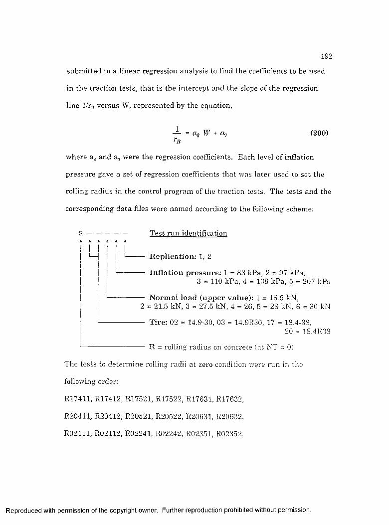
1 9 2
subm itted to a linear regression analysis to find the coefficients to be used
in the traction tests, th a t is the in tercept and the slope of the regression
line 1/rR versus W, represented by the equation,
- C g W + Gky (200)'R
where a^ and a were the regression coefficients. Each level of inflation
pressure gave a set of regression coefficients th a t was la ter used to set the
rolling radius in the control program of the traction tests. The tests and the
corresponding data files were nam ed according to the following scheme:
R▲
Test run identification
R e p lic a tio n : 1, 2
— In f la tio n p re s su re : 1 = 83 kPa, 2 = 97 kPa,3 = 110 kPa, 4 = 138 kPa, 5 = 207 kPa
— N o rm a l lo a d (u p p e r v a lu e): 1 = 16.5 kN,2 = 21.5 kN, 3 = 27.5 kN, 4 = 26, 5 = 28 kN, 6 = 30 kN
Tire: 02 = 14.9-30, 03 = 14.9R30, 17 = 18.4-38,20 = 18.4R38
'-------------------------- R = rolling radius on concrete (at NT = 0)
The tests to determ ine rolling radii a t zero condition were run in the
following order:
R17411, R17412, R17521, R17522, R17631, R17632,
R20411, R20412, R20521, R20522, R20631, R20632,
R02111, R02112, R02241, R02242, R02351, R02352,
R eproduced with perm ission of the copyright owner. Further reproduction prohibited without perm ission.
1 9 3
R03111, R03112, R03241, R03242, R03351, R03352.
Each rolling rad ius data file contained:
• On the first row,
- The filename: The data file being stored as a p rin t file, the extension
".prn" was added a t the end of the test name to obtain the filename;
- An equation giving rolling radius (RR) as a function of dynamic load:
This equation had no m eaning a t th a t point, b u t appeared because the same
data recording software was used both for rolling rad ius and traction
experim ents. The software required the two coefficients of the equation to
be entered before each test;
® On the second row, the nam es of all the variables recorded during a test:
- D1 and D2: draft loads (kN) applied to the 2 horizontal load cells (#10 in
F ig u re 43);
- V I and V2: vertical loads (kN) received by the 2 vertical load cells (#9 in
F ig u re 43);
- NL: normal (vertical) load (kN) applied by the hydraulic cylinder on the
self-leveling fram e through the load cell (#6, #7 and #5, respectively, in
F ig u re 43);
- TOR: torque (kNm) applied to the test wheel by the hydraulic motor
through the chain drive, as m easured by the torquem eter (#1, #3, #2 and #4,
respectively, in F ig u re 43);
- DFS: vertical location, w ith respect to test-wheel centerline, of the soil
R eproduced with perm ission of the copyright owner. Further reproduction prohibited without perm ission.

1 9 4
surface, as given by a small roller running on the soil surface, parallel to
the te st wheel;
- DFR: vertical location, wath respect to test-wheel centerline, of the bottom
of the test-wheel ru t, as given by a small wheel running on the bottom of
the ru t, behind the test-wheel. This data was combined w ith DFS data to
compute sinkage in some experiments;
- IPR: test-wheel inflation pressirre (kPa);
- VEL: travel velocity of the tire car (m/s);
- OMA: angular velocity of the test wheel with respect to the tire car
(rad/s);
- DIS: location of the tire car, or distance traveled along the test track (m);
- ANG: angular position of the test wheel (deg.);
- TIM: tim e (s);
- SLP: test-wheel slip {%) computed as.
OMA -SLP = I W 100
OMA
The coefficients entered at the beginning of the test, and appearing in the
equation located on the first row of the file, were used to compute the
rolling radius as a function of the dynamic load DL;
R eproduced with perm ission of the copyright owner. Further reproduction prohibited without perm ission.

1 9 5
- DL: dynamic load (kN), computed as,
D L = N L - (V I + V2) (202)
- NT: net traction (kN), computed as,
N T = D1 + D 2 (203)
- TE: tractive efficiency, computed as,
T E = (204)O M A T O R
and therefore not expressed as a percentage. Notice th a t slip and tractive
efficiency values had no meaning in the rolling radius files. Slip was
computed with arb itrary coefficients th a t had to be used as inputs for the
equation located on the first row of the file for the data recording software
to run. In fact, slip and tractive efficiency were both assum ed to be zero,
according to the choice of zero condition (self-propelled wheel on a hard
surface) and rolling radius was computed as:
_L = (205)V E L
The top 7 records of file R03242.PRN are shown in T ab le G l, A p p e n d ix G.
T ab le 18 presents the results from the rolling radius tests.
All the slope values were positive, indicating th a t rolling radius
decreased as load increased. Also, for each tire, except 18.4R38 tire #20, the
R eproduced with perm ission of the copyright owner. Further reproduction prohibited without perm ission.

1 9 6
slope decreased as in flation pressure increased, thus ind icating th a t the
effect o f load on rolling radius decreased as in flation pressure increased .
Table 18. Inverses of Rolling Radius Versus Dynamic Load, Measured on Concrete
TireInflationpressure
(kPa)
Rolling radius coefficients (l/r^ = intercept + slope * W)
Intercept (m' ) Slope (kN *m‘ )
14.9-30 #2 83 1.379 0.0078914.9-30 #2 138 1.374 0.0053114.9-30 #2 207 1.381 0.0032314.9R30 #3 83 1.396 0.0045114.9R30 #3 138 1.386 0.0033014.9R30 #3 207 1.393 0.0023618.4-38 #17 83 1.124 0.0044618.4-38 #17 97 1.123 0.0035618.4-38 #17 110 1.128 0.0035518.4R38 #20 83 1.140 0.0020918.4R38 #20 97 1.141 0.0021918.4R38 #20 110 1.149 0.00165
The indoor soil bin containing Norfolk sandy loam was prepared while
rolling radius m easurem ents were performed. The soil was first roto-tilled
to a depth of about 0.30 m and then compacted by 8 passes of the V-packer
(4 passes in one transverse position, and 4 other passes straddling the first
ones by h a lf the pitch of the packer’s wheels). The soil was then leveled
with a scraper blade. This procedure gave a fairly firm soil, w ith minimum
preparation and lead time. Tires 14.9-30 #2 and 14.9R30 #3 were tested in
the soil bin in 1/2 day, including one tire change. The soil bin was prepared
again the sam e way as for the first set of tests (1/2 day). Tires 18.4-38 #17
R eproduced with perm ission of the copyright owner. Further reproduction prohibited without perm ission.

1 9 7
and 18.4R38 #20 were tested w ithin a day. Locations of the te s t plots on
the soil bin for tires 14.9-30 #2 and 14.9R30 #3 (T ab le 19), and for tires
18.4-38 #17 and 18.4R38 #20 (T ab le 20) were randomized with a
spreadsheet random ization routine. Test plots and corresponding data files
were nam ed according to the following scheme:
— — ----- Plot identification
H R ep lica tio n : 1, 2, 3, 4
In f la tio n p re s su re : 1 = 83 kPa, 2 = 97 kPa,3 = 110 kPa, 4 = 138 kPa, 5 = 207 kPa
Slip: L = 7.5%, H = 15%, T = 20%, V = 25%
T ire : 02 = 14.9-30, 03 = 14.9R30, 17 = 18.4-38,20 = 18.4R38
Soil p re p a ra t io n : 1 = first time, 2 = second time
After each soil preparation, soil samples were taken throughout the soil
bin after each soil bin preparation, and before-traffic cone index was
m easured a t 30 evenly spaced locations, 5 rows along the soil bin, and 6
m easurem ents per row across the soil bin. T ab le s G2 a n d G3, A p p e n d ix
G, contain the filenames of the cone index m easurem ents for the first and
second soil preparations, respectively, according to their location. The
contents of the cone index data files are also described in A p p en d ix G.
F ig u re 44 shows a plot of the cone index vs. depth for one tj’pical reading.
R eproduced with perm ission of the copyright owner. Further reproduction prohibited without perm ission.

198
T a b le 19. T e s t P lo t L o c a tio n s fo r th e F i r s t S o il B in P re p a ra t io n , N o rfo lk S a n d y L oam , V-W heel P a c k ed , S u rfa c e L ev e led W ith S c ra p e r B lad e
1.32 m 2.12 m 2.92 m 3.72 m 4.52 m102H52207 kPa 27.5 kN 15%
103H42 138 kPa21.5 kN 15%
103H14 83 kPa16.5 kN 15%
103L1383 kPa 16.5 kN 7.5%
102L12 83 kPa16.5 kN 7.5%
102H42 138 kPa 21.5 kN 15%
102L42 138 kPa 21.5 kN 7.5%
103V52 207 kPa27.5 kN 25%
103V11 83 kPa16.5 kN 25%
103V51207kPa27.5 kN 25%
103V41 138 kPa21.5 kN 25%
103L12 83 kPa 16.5 kN 7.5%
103H52 207 kPa 27.5 kN 15%
102L52 207 kPa 27.5 kN 7.5%
102H12 83 kPa 16.5 kN 15%
103L52 207 kPa 27.5 kN 7.5%
103L42 138 kPa 21.5 kN 7.5%
102H41 138 kPa 21.5 kN 15%
102L41 138 kPa 21.5 kN 7.5%
103H51 207 kPa 27.5 kN 15%
103H11 83 kPa 16.5 kN 15%
102L11 83 kPa 16.5 kN 7.5%
103L11 83 kPa 16.5 kN 7.5%
103H12 83 kPa 16.5 kN 15%
103L41 138 kPa 21.5 kN 7.5%
102H51 207 kPa 27.5 kN 15%
102L51 207 kPa 27.5 kN 7.5%
103H41 138 kPa 21.5 kN 15%
103H13 83 kPa 16.5 kN 15%
103L51 207 kPa 27.5 kN 7.5%
102H1183 kPa16.5 kN 15%
Nt
R eproduced with perm ission of the copyright owner. Further reproduction prohibited without perm ission.
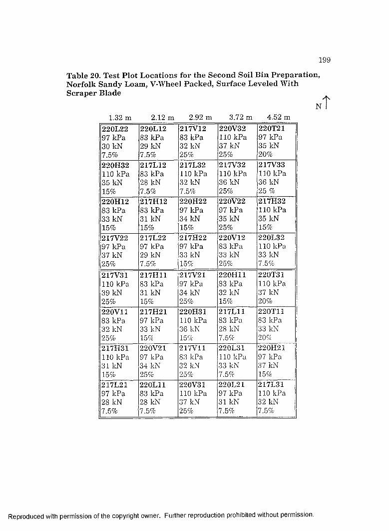
1 9 9
T ab le 20. T e s t P lo t L o c a tio n s fo r th e S eco n d S o il B in P r e p a ra t io n , N o rfo lk S a n d y Loam , V-W heel P a c k ed , S u rfa c e L ev e led W ith S c ra p e r B lade
n T1.32 m 2.12 m 2.92 m 3.72 m 4.52 m
220L22 97 kPa 30 kN 7.5%
220L1283 kPa 29 kN 7.5%
217V1283 kPa 32 kN 25%
220V32 110 kPa 37 kN 25%
220T21 97 kPa 35 kN 20%
220H32 110 kPa 35 kN 15%
217L12 83 kPa 28 kN 7.5%
217L32 110 kPa 32 kN 7.5%
217V32 110 kPa 36 kN 25%
217V33 110 kPa 36 kN 25 %
220H12 83 kPa 33 kN 15%
217H12 83 kPa 31 kN 15%
220H22 97 kPa 34 kN 15%
220V22 97 ItPa 35 kN 25%
217H32 110 kPa 35 kN 15%
217V22 97 kPa 37 kN 25%
217L22 97 kPa 29 kN 7.5%
217H22 97 kPa 33 kN 15%
220V12 83 kPa 33 kN 25%
220L32 110 kPa 33 kN 7.5%
217V31 110 kPa 39 kN 25%
217H11 83 kPa 31 kN 15%
217V21 97 kPa 34 kN 25%
220H11 83 kPa 32 kN 15%
220T31 110 kPa 37 kN 20%
220V11 83 kPa 32 kN 25%
217H21 97 kPa 33 kN 15%
220H31 110 kPa 36 kN 15%
217L11 83 kPa 28 kN 7.5%
220T11 83 kPa 33 kN 20%
217H31 110 kPa 31 kN 15%
220V2197 kPa 34 kN 25%
217V11 83 kPa 32 kN 25%
220L31 110 kPa 33 kN 7.5%
220H21 97 kPa 37 kN 15%
217L21 97 kPa 28 kN 7.5%
220L11 83 kPa 28 kN 7.5%
220V31 110 kPa 37 kN 25%
220L21 97 kPa 31 kN 7.5%
217L31 110 kPa 32 kN 7.5%
R eproduced with perm ission of the copyright owner. Further reproduction prohibited without perm ission.

200
- 0.1
■03
- 0.4
- 0-5
500 15000 2000lOOO 2500
CONE INDEX (kPA)
F igu re 44. C one in d ex versus depth curve, N orfolk Sandy Loam , V -w heel packed , surface leveled w ith scrap er b lade.
All cone index vs. depth plots were similar, with an sharp increase in
cone index in the top 60 to 80 mm, followed by a decrease to a depth of
about 350 mm, and another sharp increase due to the hardpan rem aining
below the working depth of the roto-tiller. T ab le 21 contains the average
values, s tandard deviations and coefficients of variability (CV) for both soil
preparations, and the overall values. Tip penetration speed was also
reported because cone index m easurem ents generally increase with tip
speed. Average tip speed was higher for the first soil preparation, which
partly explains the higher cone index values obtained, soil preparation being
the other possible cause for variations. The difference between average cone
index values for the two soil preparations was only 3%. Thus, the overall
R eproduced with perm ission of the copyright owner. Further reproduction prohibited without perm ission.

2 0 1
average value of 862 kPa was retained as average cone index value for the
top 150 mm layer.
T able 21. A verage V alue, S tandard D ev ia tion and C oeffic ien t o f V ariation o f C one Index and Tip Speed.
C one In dex (kPa) Tip P en etra tio n S p eed (mm/s)
F irst so il prep.
S econd so il prep.
O verall F irst so il prep.
Secon d so il prep.
O verall
Average 875 849 862 51 45.3 48.1S tandarddeviation
74 86 82 5 5.1 5.8
C.V. (%) 8.5 10.1 9.5 9.8 11.3 12.1
Dry bulk density and moisture content were also m easured in 6 different
places throughout the soil bin, after each soil preparation. At a depth of
120 to 180 mm, average dry bulk density was 1639 kg/m^ and 1601 kg/m^,
and average m oisture content was 6.28% and 5.67% for the first and second
soil preparations, respectively.
T raction D ata C ollected
The structure of the traction data files was sim ilar to th a t of the rolling
radius files, except th a t the equation for rolling radius as a function of
dynamic load, entered on the first row, besides the filename, was now used
as a prelim inary inpu t for calculations of slip and tractive efficiency. This
equation was obtained through linear regression analysis on the rolling
radius data obtained on concrete under sim ilar load and inflation pressure
conditions. The top 7 records of file 103h42.prn are shown in T ab le G4,
R eproduced with perm ission of the copyright owner. Further reproduction prohibited without perm ission.

2 0 2
A p p e n d ix G, as an example. The sinkage m easuring system did not work
well in some of the tests and was ignored during the final tests, hence the
disappearance of the DFS and DFR columns as shown in the top 7 records
of file 220h32.prn (T ab le G5, A p p en d ix G).
R eproduced with perm ission of the copyright owner. Further reproduction prohibited without perm ission.
RESULTS AND DISCUSSION
Static Experiments
For each load-deflection curve, a linear regression analysis was made,
assum ing th a t deflection was a linear function of load. All R“ values for the
regression lines were above 0.95. Stiffness was computed as the inverse of
the slope of the load-deflection curve. The regression lines had a non-zero
in tercept in all cases. This can be explained by the higher slope of the load-
deflection curve near the origin, probably due to a very small contact area,
when only the lugs started to come in contact with the load scale. The
in tercept was not determ ined because only the slope of the deflection versus
load curve was of in terest in stiffness calculations. The radial tires had a
cylindrical (ra ther than toroidal) envelope shape, particularly in the tread
area. Consequently, the whole width of the radial tires would make contact
a t once w ith the load scale; Bias-ply tires tended to enter in contact on
their centerline first, the contact area then widening until it extended to the
whole tire width.
A second regression analysis was made to relate stiffness to inflation
pressure, assum ing linearity between the two variables (F ig u re 45). The
equation of the regression line gave stiffness as a function of inflation
pressure. L inear regression analysis indicated th a t static stiffness could be
203
R eproduced with perm ission of the copyright owner. Further reproduction prohibited without perm ission.
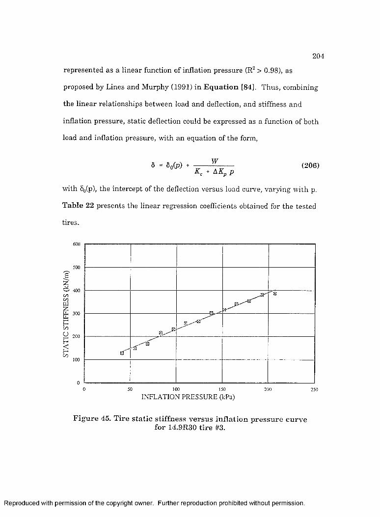
2 0 4
represented as a linear function of inflation pressure (R‘ > 0.98), as
proposed by Lines and M urphy (1991) in E q u a tio n [84]. Thus, combining
the linear relationships between load and deflection, and stiffness and
inflation pressure, static deflection could be expressed as a function of both
load and inflation pressure, with an equation of the form.
Ô = Ô q ( p ) +W (206)
with 5o(p), the intercept of the deflection versus load curve, varying w ith p.
T ab le 22 presents the linear regression coefficients obtained for the tested
tires.
600
500
c
IGOGO
zpGOu
Ic/5
400
300
200
100
' 'â
50 100 150
INFLATION PRESSURE (kPa)200 250
F ig u re 45. T ire s ta t ic s tiffn e ss v e rsu s in f la tio n p re s s u re c u rv efo r 14.9R30 t ir e #3.
R eproduced with perm ission of the copyright owner. Further reproduction prohibited without perm ission.

205
Table 22. L inear R egression Coefficients for Static Stiffness Versus Inflation Pressure Curves
Tire Max.P(kPa)
Intercept K s t a t vs. p (kN/m)
Slope K s t a t vs. p (N/m Pa)
R"K s t a t V S . P
14.9-30 #1 221 82.28 1.38 0.99614.9-30 #2 221 100.27 1.50 0.99214.9R30 #3 207 68.90 1.61 0.98816.9-30 #5 124 60.15 1.66 0.98616.9R30 #7 165 88.62 1.57 0.99518.4-30 #9 138 55.29 1.87 0.98915.5-38 #11 138 55.77 1.76 0.99015.5-38 #13 138 61.14 1.69 0.98416.9-38 #15 124 62.51 1.66 0.99918.4-38 #17 110 40.21 1.49 0.99818.4R38 #20 124 53.48 2.06 0.996
No general trend appeared from these results, with respect to tire size
or inflation pressure. Values of static stiffness ranged from 101.3 kN/m
(18.4-38 #17 a t 41 kPa inflation pressure) to 431.8 kN/m (14.9-30 #2 a t 221
kPa inflation pressure). These values were of the same order of m agnitude
as found in the literature. For each tire, static stiffness was computed for 3
inflation pressures: 41 kPa, 83 kPa, and rated inflation pressure. The 83
kPa to ra ted inflation pressure range represented the recommended range
of inflation pressures, while the 41-83 kPa range was investigated because
of the trend towards using lower inflation pressures to avoid soil compaction
(T ab le 23).
R eproduced with perm ission of the copyright owner. Further reproduction prohibited without perm ission.

2 0 6
Table 23. Com puted Static Stiffness at Various Inflation PressuresTire Rated inflation
pressure (kPa)
Mass(kg)
Static stiffness (kN/m) at
41 kPa 83 kPa rated infl. pressure
14.9-30 #1 221 73.9 138.8 196.7 387.014.9-30 #2 221 73.9 161.8 224.8 431.814.9R30 #3 207 94.3 135.0 202.8 402.816.9-30 #5 124 62.1 128.2 197.8 266.016.9R30 #7 165 113.1 152.9 218.7 347.218.4-30 #9 138 82.7 131.8 210.2 312.815.5-38 #11 138 59.9 127.7 201.4 298.015.5-38 #13 138 63.0 130.4 201.3 294.216.9-38 #15 124 78.9 130.5 200.2 268.218.4-38 #17 110 95.0 101.3 163.9 204.118.4R38 #20 124 142.4 137.8 224.1 308.4
C om parison B etw een Sam e-S ize T ires
Tires 14.9-30 #1 and #2, and 15.5-38 #11 and #13 were examples of
stiffness differences between like tires. Tires #1 and #2 had a 23.0 kN/m
(17%) stiffness difference a t 41 kPa inflation pressure, and 44,8 kN/m (12%)
a t 221 kPa, the ra ted inflation pressure. The average stiffness difference
between the two tires over the range of inflation pressures studied was 14%.
Sim ilar calculations for tires #11 and #13 lead to a 2% average stiffness
difference. The large difference observed for tires #1 and #2 suggested th a t
identical tires could have large differences in stiffness, or th a t another
variable, such as am bient tem perature during the experiment, was
significant, because the tires were tested a t different times of the year.
R eproduced with perm ission of the copyright owner. Further reproduction prohibited without perm ission.

207
Other significant factors could be the m anufacturing process, or physical
properties of the m aterials of the tires.
B ias V ersu s R adia l C onstruction C om parison
Radial and bias-ply tires were compared size by size. Tire 14.9-30 #2
had a higher stiffness than tire 14.9R30 #3. Surprisingly, a t the same
inflation pressure, radial tires 14.9R30 #3, 16.9R30 #7 and 18.4R38 #20
appeared stilTer th an bias-ply tires 14.9-30 #1, 16.9-30 #5 and 18.4-30 #17,
respectively. The tractive advantage of radial tires was often justified by
their higher flexibility, which gave a larger footprint, and by the ir belt,
which did not stretch and thus m aintained a fairly constant rolling radius,
independent of dynamic load. The argum ent of increased flexibility did not
seem to hold for the tires tested. A look a t weight and rated inflation
pressure helped understand the differences in stiffness. Additional weight
could be required for two reasons; stronger, thicker, carcass required to
w ithstand a higher inflation pressure and thus carry a heavier load; and
different construction for radial tires. For example, tire 14.9R30 #3 was
20.4 kg (28%) heavier than 14.9-30 tire #2. This was apparently related to
construction differences (bias vs. radial) because the two tires had only a
small difference in rated inflation pressure (14 kPa). The 16.9R30 tire #7
was 51.0 kg (82%) heavier than 16.9-30 tire #5, with a 41 kPa higher rated
inflation pressure, and 18.4R38 tire #20 was 47.4 kg (50%) heavier than
18.4-38 tire #17, w ith a 24 kPa higher rated inflation pressure. The
R eproduced with perm ission of the copyright owner. Further reproduction prohibited without perm ission.

208
following 3 variables seem im portant for static stiffness comparisons:
- tire size,
- ra ted inflation pressure, and
- construction.
C om p arison B etw een T ires o f D ifferen t W idth
Tires 14.9-30 #1 and #2, 16.9-30 #5 and 18.4-30 #9 represented 3
different section widths for the 30 inch rim diam eter category, while tires
15.5-38 #11 and #13, 16.9-38 #15, and 18.4-38 #17 represented the 38 inch
rim diam eter category. Tires seemed to range according to ra ted inflation
pressure, ra th e r than section width, w ithin each category. Stiffness
increased w ith rated inflation pressure, bu t no general trend could be
observed concerning the effect of width. The effect of width, if any, was
hidden by the effect of rated inflation pressure.
D ynam ic E x p erim en ts
Linear regression coefficients were computed both for the dynamic
stiffness and damping coefficient versus inflation pressure curves. T ab le
24 presents these coefficients for the tested tires. F ig u re 46 shows the
dynamic stiffness and damping coefficient versus inflation pressure curves
for 14.9R30 tire #3. Tires 16.9-30 #5 and 18.4-38 #17 had the lowest
dam ping coefficients (lowest intercepts and lowest slopes), th a t is the lowest
phase angles (|)f between force and deflection. This made the computation of
Cj, according to E q u a tio n [193], less accurate (lower values).
R eproduced with perm ission of the copyright owner. Further reproduction prohibited without perm ission.

2 0 9
Table 24. Linear Regression Coefficients for Dynamic Stiffness and Damping Coefficent Versus Inflation Pressure Curves
Tire Max.P(kPa)
Interc.Kuy.V S. p(kN/m)
Slope Kdy. vs. p(N/m Pa)
R2Key.V S. p
Interc. Cj vs. p (s kN/m )
Slope Cd vs. p (sin)
R"Cd vs. P
14.9-30 #1 221 112.50 2.00 0.999 7.45 0.04 0.90114.9-30 #2 221 123.78 2.32 0.999 14.00 0.10 0.94814.9R30 #3 207 90.70 2.00 0.998 6.89 0.05 0.92116.9-30 #5 124 91.76 2.58 1.000 5.25 0.02 0.73116.9R30 #7 165 111.24 2.18 0.997 9.30 0.05 0.94418.4-30 #9 138 87.19 2.77 0.999 6.22 0.03 0.81015.5-38 #11 138 80.89 2T2 0.996 T69 0.10 0.97815.5-38 #13 138 84.67 &83 0.999 7.98 0.14 0.89616.9-38 #15 124 96.44 &78 0.999 7.44 0.04 0.86018/L38 #17 110 123.19 &98 0.999 5.69 0.02 0.64018.4R38 #20 124 109.11 2.63 0.998 6T8 0.03 0.942
600
^ 500
§0000UJZu.llp00u
400
300
200
< z > 100 a
. . . . . A - ". . - A
r - A - ....
A " - "
A
à
. 6
. - ■ A
A
■■ + - r+ + + . + + +
- r
, , ,
+ - r r
1
0 50 100 150
INFLATION PRESSURE (kPa) A DYNAMIC STIFFNESS (kN/m)
200
60
50
40
30
10
250
Z
uEu.wOuozEs<Q
+ DAMPING COEFFICIENT (s.kN/m)
F igu re 46. T ire dynam ic stiffn ess and dam ping co effic ien t versu s in fla tio n p ressu re cu rves for 14.9R30 tire #3.
R eproduced with perm ission of the copyright owner. Further reproduction prohibited without perm ission.

2 1 0
Dynamic values of stiffness appeared to be h igher than static values.
For example, a t 207 kPa inflation pressure, tire 14.9R30 #3 had an average
dynamic stiffness of 504.5 kN/m over the 0.76-1.41 Hz frequency range,
versus a 402.8 kN/m static stiffness. This showed the im portance of
d^mamic m easurem ents for the development of tire models. Ratios of
dynamic stiffness to static stiffness were computed over the norm al
utilization range of the tires, from 83 kPa to ra ted inflation pressure (T able
25). Because both the static and the dynamic stiffnesses varied linearly
w ith inflation pressure, while the ir ratio changed only slightly over the
p ressure range considered, only an average value of the ratio was retained,
T ab le 25. R a tio s o f D y n am ic S tiffn e ss to S ta tic S tiffn e ssT ire K dyÆ tat
r a t io a t S3 k P a in f la tio n p re s s u re
Kdyn/fRstat r a t io
a t r a te d in f la tio n p re s s u re
A v e rag eKjy/K^tat
r a t io o v e r th e 83 k P a to r a te d
in f la tio n p re s s u re r a n g e
R e la tiv ed iffe re n c e
(%)
14.9-30 #1 1.414 1.430 L422 +4214.9-30 #2 1.407 1.474 1.441 +4414.9R30 #3 L265 T252 1.259 +2616.9-30 #5 1.546 T548 1.547 +5516.9R30 #7 T335 T355 1.345 +3518.4-30 #9 1.507 1.499 T503 +5015.5-38 #11 T522 1.531 1.527 +5315.5-38 #13 L586 1.614 1.600 +6016^h38 #15 L633 1.644 1.639 +6418.4-38 #17 &261 2.210 2.236 + 12418.4R38#20 1.459 T409 L434 +43
R eproduced with perm ission of the copyright owner. Further reproduction prohibited without perm ission.

2 1 1
thus giving an average value of the relative difference between the two
stiffnesses. Relative differences ranged from 26% to 124%. This wide range
of variation showed th a t static stiffness values should not be used as
indicators of dynamic stiffness. The only definite trend appearing here was
th a t dynamic stiffness was consistently higher than static stiffness. This
should be taken into consideration when building models, particularly those
related to vertical vibrations.
No correlation was found between the frequency of oscillation and the
values of and C^, bu t the frequency range was limited to 0.363-1.461 Hz
by the hydraulic power supply (agricultural tractor) used during the
experiments. Rolling circumferences a t rated load and inflation pressure of
14.9-30 and 18.4R38 tires are 4.293 m and 5.283 m (T able C2, A p p en d ix
C), respectively. Field speeds corresponding to the highest pull values are
generally between 5 and 8 km/h (plowing, cultivating), thus requiring
angular velocities in the ranges of 0.324-0.518 rev/s and 0.263-0.421 rev/s
for 14.9-30 and 18.4R38 tires, respectively. These angular velocities can be
compared to the te s t frequencies because a point located on the surface of a
tire is deflected for each revolution of the tire. The range of test frequencies
covered p a rt of the normal ranges of operating frequencies con-esponding to
the 5-8 km /h field speed range. No natural frequencies were encountered
during the tests.
R eproduced with perm ission of the copyright owner. Further reproduction prohibited without perm ission.

2 1 2
Both Kjy„ and decreased w ith inflation pressure, Kjy„ tended to
increase w ith frequency and to decrease. Values of Kjy„ observed ranged
from 101.3 kN/m to 636.5 kN/m, and values of from 6.2 kN.s/m to 36.1
kN.s/m.
Note th a t both the static and dynamic experim ents were done under
non-rolling conditions. Stiffness values, and the ir trends (linearity with
inflation pressure, dynamic values higher th an static values), m ay also be
affected by rolling conditions, because of differences in deformation modes.
T a b le s 26 a n d 27 contain dynamic stiffness and dam ping coefficient values
computed a t three levels of inflation pressure. The damping coefficient
values tended to decrease with rated inflation pressure, ra th e r th an mass.
T a b le 26. C o m p u te d D ynam ic S tiffn ess a t V a rio u s In f la tio n P r e s s u r e s
T ire R a te din f la tio np re s s u re
(kP a)
M ass(kg)
D y n am ic s tiffn e ss (kN/m) a t
41 k P a 83 k P a r a te d infl. p re s s u re
14.9-30 #1 221 7&9 194.3 27&2 5&T614.9-30 #2 221 7&9 21&9 316 3 63&514.9R30 #3 207 9 4 ^ 172.7 25&6 504^16.9-30 #5 124 62.1 197.5 30n8 411.616.9R30 #7 165 113.1 200.6 29&0 470.618.4-30 #9 138 8&7 20&6 31&8 46&015.5-38 #11 138 59.9 19&4 30&6 456T15.5-38 #13 138 6&0 200.5 31&2 474.716.9-38 #15 124 78.9 21&3 32&9 44^818.4-38 #17 110 95.0 2 45^ 37&6 451.118.4R38 #20 124 14&4 216.7 327.0 43443
R eproduced with perm ission of the copyright owner. Further reproduction prohibited without perm ission.
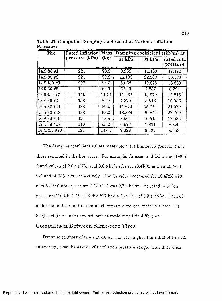
2 1 3
Table 27. Computed Damping Coefficient at Various Inflation Pressures
Tire Rated inflation pressure (kPa)
Mass(kg)
Damping coefficient (skN/m) at41 kPa 83 kPa rated infl.
pressure14.9-30 #1 221 73.9 9.252 11.100 17.17214.9-30 #2 221 73.9 18.100 22.300 36.10014.9R30 #3 207 94^ 8.862 10.878 16.83016.9-30 #5 124 62.1 6.229 7.237 8.22116.9R30 #7 165 113.1 11.263 13.279 17.21518.4-30 #9 138 8&7 7.370 8.546 10.08615.5-38 #11 138 59.9 11.670 15.744 21.07915.5-38 #13 138 63.0 13.838 19.844 27.70916.9-38 #15 124 78.9 8.961 10.515 12.03218.4-38 #17 110 95.0 &673 7.681 &32918.4R38 #20 124 142.4 7.329 &505 ff653
The dam ping coefficient values m easured were higher, in general, than
those reported in the literature. For example, Janssen and Schuring (1985)
found values of 2.8 s-kN/m and 3.0 s kN/m for an 18.4R38 and an 18.4-38
inflated a t 138 IcPa, respectively. The Cj value m easured for 18.4R38 #20,
a t ra ted inflation pressure (124 kPa) was 9.7 skN /m . At rated inflation
pressure (110 kPa), 18.4-38 tire #17 had a Cj value of 8.3 s kN/m. Lack of
additional da ta from tire m anufacturers (tire weight, m aterials used, lug
height, etc) precludes any attem pt a t explaining this difference.
C om parison B etw een Sam e-S ize T ires
Dynamic stiffness of tire 14.9-30 #1 was 14% higher than th a t of tire #2,
on average, over the 41-221 IcPa inflation pressure range. This difference
R eproduced with perm ission of the copyright owner. Further reproduction prohibited without perm ission.

2 1 4
was identical to th a t observed for static stiffness. Tire 15.5-38 #13 showed
a 4% h igher dynamic stiffness than tire #11, on average, for the 41-138 kPa
inflation pressure range. This difference was close to the 2% difference
observed under static conditions. This suggested th a t comparisons made
under static conditions could be extrapolated to dynamic conditions. The
large difference observed for the 14.9-30 tires (14%) pointed out the
im portance of variations among sim ilar tires when sim ulating a vehicle’s
behavior.
Concerning dam ping coefficient, large differences were observed between
sim ilar tires. Tire #2 showed a value of Cj approximately twice th a t of tire
#1 a t all inflation pressures investigated. Damping coefficient for tire #13
was an average of 25% higher th an th a t of tire #11. Also, tire #11 was a
year older th an tire #13. As rubber tends to "dry out" and become stiffer
w ith age, stiffness should have increased with age for these unused tires,
thus m aking the difference between tires #11 and #13 even larger. These
large potential differences may prove significant, especially when using tire
models in vehicle dynamics simulations.
B ia s V ersus R adia l C on stru ction C om parison
U nder dynamic conditions, tires 14.9-30 #1 and #2 were 8% and 23%
stiffer, respectively, on average, than tire 14.9R30 #3, over the 41-207 kPa
inflation pressure range. Tire 16.9-30 #5 was 3% stiffer than 16.9R30 #7,
on average, over the 41-124 IcPa range, and tire 18.4-38 #17 was 15% stiffer
R eproduced with perm ission of the copyright owner. Further reproduction prohibited without perm ission.

2 1 5
than 1S.4R38 #20, on average, over the 41-110 kPa range. Therefore, bias-
ply tires appeared stiffer than radiais under dynamic conditions. Moreover,
radiais had higher ra ted inflation pressures th an th e ir bias-ply counterparts
in the 16.9 x 30 and 18.4 x 38 sizes. This m eant stronger carcasses for the
radiais, and thus a larger weight, bu t not more rigidity.
Tires #5 and #17 (bias-ply) showed lower Cj values th an tires #7 and
#20 (radial), respectively, but the radiais had higher rated inflation
pressures, and therefore larger m ass, than their bias-ply counterparts. The
effect of ra ted inflation pressure and m ass probably m asked the assessm ent
of construction effects. Radial tire #3, though, had a lower Cj value than
bias-ply tires #1 and #2, although its mass was larger. Rated inflation
pressure was lower for tire #3, which m eant a th inner, more flexible,
carcass, w ith a thicker belt-tread area, because of the radial construction.
C om parison B e tw een T ires o f D ifferen t W idth
Tires of the same rim size but different section width were assembled
into two groups; 30 inch rim diam eter, and 38 inch rim diam eter (T ab les 28
a n d 29).
Rated inflation pressure decreased when section width increased,
implying th a t the narrow er tires should have been stiffer because they were
built w ith stronger carcasses to w ithstand higher pressures. However,
dynamic stiffness increased with section width, despite the decrease in
inflation pressure rating. Therefore, stiffness increased with tire width.
R eproduced with perm ission of the copyright owner. Further reproduction prohibited without perm ission.

2 1 6
Table 28. Values of at 41 and 124 kPa Inflation Pressure for 30- Inch Rim Tires
Tire Kjyo (41 kPa) Kdy. (124 kPa) Rated inflation pressure (kPa)
14.9-30 #1 194.3 360.5 22114.9-30 #2 218.9 411.5 22116.9-30 #5 197.5 411.6 12418.4-30 #9 200.6 430.7 138
Table 29, Values of Kjy„ at 41 and 110 kPa Inflation Pressure for 38- Inch Rim Tires
Tire Kdy. (41 kPa) Kjy„ (110 kPa) Rated inflation pressure (kPa)
15.5-38 #11 192^ 380.1 13815.5-38 #13 200.5 396.0 13816.9-38 #15 210.3 402L2 12418.4-38 #17 24&4 451.1 110
Note th a t m ass also increased with tire width, in general, because of the
additional m aterial required to build wider tires. This probably contributed
to the increase in stiffness.
Obseiwation of the damping coefficient regression coefficients suggested
th a t damping coefficient increased with rated inflation pressure (and
thickness of the carcass, as shown by the values of mass) and decreased
with width. However, the two effects could not be assessed more closely as
they opposed each other.
Most of the compaidsons made here involved rated inflation pressure,
and, consequently, m ass and carcass thickness. However, the
thermodynamic properties of the a ir trapped inside a tire should also be
R eproduced with perm ission of the copyright owner. Further reproduction prohibited without perm ission.

2 1 7
considered. Inflation pressure was m aintained constant during traction
experim ents, bu t was not during static and dynamic experiments, because
the instrum entation used for the la tte r did not allow for pressure control.
Consequently, during static experiments, small variations of inflation
pressure were observed, when loading the tires, hut the instrum entation
available did not allow an accurate recording of these variations. The air
pressure gage used was m anual and was m arked only every 1 psi (6.895
kPa). However, the largest variations reached about 8.6 kPa for tire #2 a t
221 kPa inflation pressure, when going from zero to maximum load. This
represented a variation of about 4% in air pressure. An additional test was
performed with the same tire to evaluate the change in in ternal volume of
the tire with inflation pressure. For that, the tire was carefully inflated
w ith w ater only. W ater pressure and volume of w ater injected were
recorded. Considering w ater as incompressible, the variation in in ternal
volume could he computed. At 83 kPa w ater pressure, the in ternal volume
was 271 1 (0.271 nP). At 221 kPa, the volume was 286 1 (0.286 nP). This
represented a variation of 5.5% in volume (15 1) for a 138 kPa change in
inflation pressure. Therefore, a 8.6 kPa change in inflation pressure would
have implied a 0.9 1 change in in ternal volume (0.3%). An adiabatic,
reversible transform ation of air w ithin the tire can be assumed, thus
following the equation (Emswiler and Schwartz, 1943),
R eproduced with perm ission of the copyright owner. Further reproduction prohibited without perm ission.

2 1 8
P a b s = constant (207)
where:
p„bs = absolute a ir pressure (Pa), and
V = volume of a ir (m^).
According to this equation, tire in ternal volume should have been reduced
by 8% to increase a ir pressure by 8.6 kPa, starting a t 221 kPa. This
suggests a change in tire in ternal volume under the effect of load, volume
being reduced by about 8% for an increase of a ir gage pressure by about 4%
in the given conditions (14.9-30 tire initially a t 221 kPa gage inflation
pressure).
All the tires were new. Effect of service duration should be considered.
For example, the same tires could be tested again after a certain num ber of
hours in operation to investigate the effects of the repeated cyclic loading
encountered in service.
An in teresting comparison could be made between the largest and the
sm allest tires tested (14.9-30, 14.9R30, 18.4-30 and 18.4R38). At 110 kPa
inflation pressure, the large tires have a higher load capacity than the the
sm aller tires inflated a t 207 kPa. For the same load, this implies a much
higher average contact pressure for the small tires than for the large ones,
because of the differences in contact area and inflation pressure. Therefore,
the sm aller tires seem more appropriate for road service, while the larger
tires should be recommended for field service, because of reduced
R eproduced with perm ission of the copyright owner. Further reproduction prohibited without perm ission.

2 1 9
compaction and improved flotation. The higher dam ping coefficient of the
14.9 X 30 tires would also help improve tractor ride a t road speeds.
Traction Experiments
Two im portan t observations were made during the experiments:
- The tracks left by the tires in the soil bin had different appearances,
depending on the carcass construction of the tire. The w idth of the tracks
left by the bias-ply tires increased with load, reaching full w idth a t some
point during loading. The tracks left by the radial tires were alm ost always
full width, even a t low load. This was probably due to the belt of the radial
tires, which gave a cylindrical, ra th e r than toroidal, shape to the tread area
of the tire. This geometric difference was pointed out by earlier researchers
by showing the difference in contact area between the two carcass
constructions. On a hard surface, radiais offered a ra th e r rectangular
contact area, while bias-ply tires gave an elliptical contact area. The whole
w idth of the radial tires contributed to traction a t all times (only the length
of the contact area changed with load), while bias-ply tires needed to reach
a certain load before their whole w idth entered in contact. This also m eant
th a t the pressure distribution under radial tires was more uniform than
under bias-ply tires.
- U nder heavy load, high torque conditions, the sidewall area of the bias-
ply tires tended to buckle. This phenomenon did not occur with radiais.
Buckling of the sidewalls has often been linked to underinflation or
R eproduced with perm ission of the copyright owner. Further reproduction prohibited without perm ission.

2 2 0
overloading in tire care literature , and was m entioned as resulting in
dam age and accelerated failure of tires, as carcass plies were subjected to
repeated excessive load cycles.
A prelim inary analysis of the data was made to evaluate the am plitude
of variation of the variables, besides vertical load, th a t were controlled
during each te st (inflation pressure IPR, slip SLP, actual travel speed VEL,
and angular velocity of the test wheel OMA). Rolling radius changed with
dynamic load, so the single-wheel tester had to modify either VEL or OMA
to m aintain the desired constant SLP. Assuming th a t both IPR and VEL
rem ained constant during a test, the change in OMA required to m aintain a
constant SLP could be estim ated as dynamic load, DL, increased. For
example, the regression equation for rolling radius of tire 14.9-30 #2 a t 83
kPa inflation pressure was
— = 1.379 + 0.00789 *DL (208)
Therefore, the rolling radius a zero dynamic load was 0.725 m, and it
decreased to 0.663 m as load increased to 16.5 kN during a test. This
represented a 9.4% decrease in r^ over the load range. Because slip was
computed as.
SLP - 1 - — ■ (209)OMA rg
then OMA had to increase by 9.4% to compensate for the change in rolling
R eproduced with perm ission of the copyright owner. Further reproduction prohibited without perm ission.

2 2 1
radius. Actually, slip had large variations (very high CV values), while both
VEL and OMA varied moderately (T ables 30 a n d 31). These variations
may have been due to the mode of operation of the control system of the
single-wheel tester, and had an im portant effect on the data collected
because slip was the major influence on traction.
Actual travel velocity was m aintained near 0.15 m/s, or 0.54 km/h, a
very low value compared to common field travel speeds of 8 km/h and above.
Previous experim ents by B urt and Lyne (1985) had shown th a t average
travel velocity had little effect on traction. V ariations in forward speed
were small enough to have no significant effect on the resu lts. Average
travel velocity rem ained practically identical from test to test, and standard
deviation and CV were low for each test. D ata from tests 103L12 and
103L13 were rejected because of technical difficulties th a t caused an
unacceptable level of scatter (high CV values).
R eproduced with perm ission of the copyright owner. Further reproduction prohibited without perm ission.

222Table 30. Variations of Inflation Pressure, Actual Speed, Angular Velocity and Slip During Tests of Tires #2 and #3
F ileIPR VEL OMA SL P
m ean std CV m ean std CV m ean std CV m ean std CVk P a k P a % m/s m/s % rad/s rad/s % % % %
102L11 83.23 0.47 0.6 0.150 0.002 1.6 0.236 0.007 2.9 7.537 2.16 28.6102L12 83.14 0.44 0.5 0.150 0.003 1.9 0.235 0.009 4 7.203 3.54 49.2102L41 138.20 0.42 0.3 0.150 0.002 1.6 0.233 0.007 3 7.329 2.58 35.3102L42 138.00 0.59 0.4 0.150 0.002 1.6 0.233 0.008 3.2 7.271 2.82 38.7102L51 207.00 0.44 0.2 0.150 0.003 2.1 0.231 0.006 2.7 7.441 2.68 36.0102L52 206.80 0.44 0.2 0.151 0.002 1.6 0.233 0.006 2.6 7.576 2.33 30.7102H11 83.50 0.59 0.7 0.151 0.004 2.9 0.255 0.009 3.4 14.690 &68 25.0102H12 83.30 0.39 0.5 0.150 0.003 2.1 0.254 0.009 3.6 14.830 3.17 21.4102H41 137.90 0.52 0.4 0.151 0.003 1.9 0.254 0.009 3.5 14.860 2.76 18.6102H42 137.90 0.39 0.3 0.150 0.003 1.9 0.252 0.008 3 14.820 2.67 18.0102H51 206.90 0.39 0.2 0.151 0.004 3.0 0.251 0.010 3.9 14.600 4.07 27.9102H52 196.30 0.38 0.2 0.150 0.004 2.4 0.252 0.009 3.6 14.970 3.24 21.G103L11 83.22 0.43 0.5 0.150 0.002 1.5 &233 0.007 2.9 7.490 2.83 37.8103L12 83.19 0.46 0.5 0.150 0.004 2.7 0.232 0.009 4 6.845 4.21 61.5103L13 8&23 0.47 0.6 0.152 0.004 2.5 0.214 0.007 3.1 -2.920 4.45 -152103L14 83.19 0.39 0.5 0.151 0.003 2.3 0.233 0.007 3.2 7.304 3.48 47.7103L41 138.10 0.48 0.3 0.150 0.004 2.8 0.230 0.010 4.1 7.442 4.14 55.7103L42 138.00 0.49 0.4 0.150 0.005 3.1 0.230 0.009 4.0 7.362 4.09 55.5103L51 206.90 0.42 0.2 0.150 0.005 3.3 0.231 0.010 4.2 7.283 4.44 61.0103L52 207.00 0.41 0.2 0.150 0.004 2.7 0.230 0.008 3.3 L234 3.62 50.1103H12 83.11 0.48 0.6 0.150 0.004 2.5 0.253 0.009 3.6 14.910 3.38 22.7103H13 83.21 0.45 0.5 0.150 0.004 3.0 0.253 0.010 4.1 15.420 3.85 25.0103H41 138.00 0.49 0.4 0.150 0.004 2.5 0.252 0.010 3.8 15.400 3.78 24.6103H42 138.00 0.50 0.4 0.150 0.003 1.8 0.251 0.009 3.4 14.950 3.14 21.0103H51 207.00 0.54 0.3 0.151 0.005 3.2 &250 0.010 4.2 14.290 4 26 2&a103H52 207.00 0.51 0.2 0.150 0.004 3.0 0.251 0.011 4.3 14.880 &99 2&8103V11 83.23 0.41 0.5 0.151 0.004 2.7 0.287 0.011 3.7 24.730 3.11 12.6103V41 137.80 0.48 0.3 0.150 0.004 2.4 0.284 0.010 3.6 25.090 2.95 11.7103V51 206,80 0.47 0.2 0.150 0.004 2.8 0.284 0.013 4.6 24.720 3.81 15.4103V52 206.90 0.50 0.2 0.150 0.005 3.4 0.285 0.015 15.3 24.830 14.40 17.7
R eproduced with perm ission of the copyright owner. Further reproduction prohibited without perm ission.

223
Table 31. Variations of Inflation Pressure, Actual Speed, Angular Velocity and Slip During Tests of Tires #17 and #20
IP R VEL OMA SLPF ile m ean std CV m ean std CV m ean std CV m ean std CV
k P a k P a % m /s m /s % rad/s rad /s % % % %
217L11 83.28 0.48 0.6 0.150 0.004 2.9 0.190 0.007 3.9 6.741 4.03 60217L12 83.44 0.47 0.6 0.150 0.004 2.6 0.190 0.007 3.7 6.820 3.87 57217L21 97.26 0.39 0.4 0.150 0.003 2.2 0.188 0.007 3.7 6.989 3.7 53217L22 97.16 0.48 0.5 0.150 0.004 2.6 0.189 0.008 4.3 7.068 3.99 56217L31 110.40 0.42 0.4 0.150 0.004 2.4 0.191 0.008 4.0 7.088 3.6 51217L32 110.30 0.43 0.4 0.150 0.004 2.6 0.190 0.008 4.3 7.087 4.02 57217H11 83.47 0.43 0.5 0.150 0.003 1.9 0.207 0.009 4.5 14.480 3.53 24217H12 83.35 0.46 0.5 0.150 0.004 2.5 0.207 0.009 4.6 14.520 3.59 25217H21 97.14 0.46 0.5 0.150 0.004 2.8 0.207 0.010 4.7 14.680 3.91 27217H22 97.24 0.45 0.5 0.150 0.004 2.4 0.205 0.008 4.1 14.420 3.48 24217H31 110.20 0.40 0.4 0.150 0.004 3.0 0.205 0.008 3.8 14.430 3.76 26217H32 110.20 0.46 0.4 0.150 0.004 2.8 0.207 0.011 5.4 14.450 4.55 32217V11 83.37 0.45 0.5 0.150 0.005 3.3 0.236 0.012 5.2 24.590 4.23 17217V12 83.45 0.38 0.5 0.150 0.004 2.4 0.235 0.014 5.9 24.440 4.49 18217V21 97.31 0.42 0.4 0.150 0.004 2.3 0.234 0.012 5.2 24.630 3.81 15217V22 97.36 0.42 0.4 0.150 0.003 2.1 0.233 0.012 5.1 24.380 3.71 15217V31 109.70 4.23 3.9 0.150 0.003 2.3 0.234 0.014 5.8 24.510 4.41 18217V32 110.30 0.45 0.4 0.150 0.004 2.4 0.233 0.012 5.0 24.040 &83 16217V33 110.30 0.41 0.4 0.150 0.004 2.8 0.235 0.014 6.0 24.540 4.42 18220L11 8&27 0.41 0.5 0.150 0.005 3.2 0.189 0.007 3.9 7.226 4.24 59220L12 83.37 0.44 0.5 0.150 0.003 2.0 0.190 0.009 4.7 7.530 A28 57220L21 97.38 0.43 0.4 0.150 0.004 3.0 0.189 0.009 4.9 7.088 4.77 67220L22 97.33 0.41 0.4 0.150 0.003 2.3 0.190 0.007 3.9 7.273 4.15 57220L31 110.20 0.40 0.4 0.150 0.003 2.1 0.189 0.007 3.7 7.017 3.64 52220L32 110.50 &39 0.3 0.150 0.004 2.9 0.190 &009 4.7 7.347 4.56 62220H11 83.53 0.46 0.5 0.150 0.004 2.4 &206 0.010 5.0 14.880 4.38 29220H12 83.32 0.41 0.5 0.150 0.004 2.3 0.205 0.009 4.6 14.590 4.26 29220H21 97.43 0.50 0.5 0.150 0.004 2.7 &206 0.011 5.1 14.430 4.62 32220H22 97.28 0.41 0.4 0.150 0.004 2.6 0.207 0.011 5.4 14.950 4.69 31220H31 110.30 0.41 0.4 0.150 0.003 2.1 0.206 0.011 5.4 14.330 4.72 33220H32 110.40 0.41 0.4 0.150 0.003 1.9 0.207 0.010 4.7 14.730 3.99 27220T21 97.53 0.42 0.4 0.150 0.004 2.4 0.221 0.015 7.0 20.150 5.46 27220T31 110.40 0.38 0.3 0.150 0.004 2.3 0.221 0.015 7.0 19.770 5.39 27220V11 83.30 0.41 0.5 0.150 0.004 2.7 0.231 0.013 5.7 24.410 4.30 18220V12 83.51 0.44 0.5 0.149 0.004 2.7 0.232 0.013 5.5 24.560 4.18 17220V21 97.44 0.51 0.5 0.150 0.004 2.5 0.234 0.015 6.5 24.710 5.16 21220V22 97.29 0.41 0.4 0.150 0.004 3.0 0.235 0.017 7.2 24.730 5.61 23220V31 110.30 0.39 0.4 0.151 0.004 2.8 0.235 0.014 6.1 24.640 4.84 20220V32 110.40 0.44 0.4 0.150 0.004 2.7 0.234 0.016 6.7 24.480 5.34 22
R eproduced with perm ission of the copyright owner. Further reproduction prohibited without perm ission.

224
R o llin g R ad iu s
Rolling rad ius versus dynamic load data showed a large scatter (F ig u re
47). A verification of the regression equations provided by the NSDL
showed th a t the values for these equations were between 0.063 and
0.386. Therefore, possible improvements on the rolling radius model were
investigated. An a ttem pt was made a t reducing the scatter by averaging
da ta by groups of 20 adjacent points (F ig u re 48). This did not prove
satisfactory, because the recomputed R^ values ranged from 0.266 to 0.850.
onDQ2OSdS
0.35
0.8
0.75
0.7
0.65
0.6
0.550 5 10 15 20
DYNAMIC LOAD, DL (kN)
F igure 47. R o llin g radius versus dynam ic load, 14.9-30 tire #2 at 83 kP a in fla tion pressure.
R eproduced with perm ission of the copyright owner. Further reproduction prohibited without perm ission.

225
0.74
0.73
0.72
0.69
g6 0.68
i -
0.66
0.65
0.640 5 10 15 20
DYNAMIC LOAD, DL (kN)
F ig u r e 48. T w e n ty -p o in t a v e r a g e s o f r o l l in g r a d iu s v e r s u s d y n a m ic lo a d , 14 .9 -30 t ir e #2 a t 83 k P a in f la t io n p r e s s u r e .
Visual observation of the rolling radius versus dynamic load curves
(F ig u re s 49 to 52) suggested th a t rolling radius could be satisfactorily
represented as a linear function of load, with the slope being a linear
function of inflation pressure. Thus,
rjj = Û6 + Oy D L (210)
where ag was a constant and a was a linear function of inflation pressure,
expressed as.
R eproduced with perm ission of the copyright owner. Further reproduction prohibited without perm ission.

226
i1§COD52 Ü
i§
0.74
0.73
0.72
0.71
0.7
0.69
0.68
0.67
0.66
0.65
V
X ,
■ x .
0 5 10 15 20 25
DYNAMIC LOAD (kN)
_B_83kPa 138 kPa _*_207kPa
F ig u r e 49. C o m p u te d r o l l in g r a d iu s v e r s u s lo a d o f 14 .9 -30 t ir e #2 a t v a r io u s in f la t io n p r e s s u r e s
30
0.74
OJ 0.73
0.72
0.71
0.7
Q 0.69
0.68
0.67
0.660 5 10 15 20 25 30
DYNAMIC LOAD (kN)
_ffl_83kPa 138 kPa 207 kPa
F ig u r e 50. C o m p u te d r o l l in g r a d iu s v e r s u s lo a d of 14 .9R 30 t ir e #3 a t v a r io u s in f la t io n p r e s s u r e s
R eproduced with perm ission of the copyright owner. Further reproduction prohibited without perm ission.

2 2 70.91'b 0.9u5 0.89C£|o 0.88Zp 0.87uz 0.86oon 0.85D5 0.84s 0.83Üs 0.82►J 0.81oC2 0.8
3!X.
0 5 10 15 2 0 25
DYNAMIC LOAD (kN)
83 kPa 97 kPa 110 kPa
F igu re 51. C om puted ro llin g rad iu s versu s load o f 18.4-38 tire #17 at various in fla tio n p ressu res
30
0.89
5gZ8Zo00D52az3jo
0.87
0.86
0.85
0.84
0.83
0 .82
0 5 10 IS 2 0 25 30
DYNAMIC LOAD (kN)
+ 83kPa _»_97 kPa - a_ 110 kPa
F igu re 52. C om puted ro llin g rad iu s versu s load o f 18.4R38 tire #20 at various in fla tio n p ressu res
R eproduced with perm ission of the copyright owner. Further reproduction prohibited without perm ission.

228
Oy = Og + Og j3 ( 2 1 1 )
w here and ag were constants. Combining the two equations provided a
linear regression equation for data computed from the regression equations
provided by the NSDL:
+ Og DL p (212)
w here ag, a and ag were the regression coefficients. This seemed a valid
assum ption, particularly for tires 14.9-30 #2 and 14.9R30 #3. This equation
gave a b e tte r fit th an E q u a tio n [210] with coefficient as a constant. It
also fitted the data be tter than an equation of the form,
~ ®io + ^11 D L + 0^2 P (213)
w ith ajo, a,i and a,., as regression coefficients.
The correlation coefficients obtained showed th a t this equation could
represen t tire rolling radius with reasonable accuracy (T able 32). Although
the model was not supported by enough tests to be validated for tires other
th an those tested, it offered the advantage of including both dynamic load
and inflation pressure as inputs. The models presented earlier by Charles
and Schuring (1984), and Brixius and Wismer (1978) did not include
inflation pressure as a variable. Also, the empirical determ ination of the
regression coefficients ag, a, and ag required the determ ination of rolling
rad ius in only three sets of conditions, such as:
- m inim um recommended inflation pressure, and zero load.
R eproduced with perm ission of the copyright owner. Further reproduction prohibited without perm ission.

229
- m inim um recommended inflation pressure, and ra ted load a t th a t
pressure,
- m axim um recommended inflation pressure, and ra ted load a t th a t
pressure.
T a b le 32. R e g re s s io n C o effic ien ts fo r R o llin g R a d iu s a s a F u n c tio n o f D y n am ic L o ad a n d In f la tio n P re s s u re
T ire ag (m) a? (mTkN) ag (m /kN k P a ) R :
14.9-30 #2 0.725157 -0.00515 0.000017 0.97814.9R30 #3 0.718375 -0.00297 9.1 X 1 0 ' 0.93818.4-38 #17 0.888442 -0.00335 3.2 X 10 ' 0.96818.4R38 #20 0.87453 -0.00119 -2.0 X 10 ' 0.959
As expected, dynamic load had a lesser effect on radial tires th an on
bias-ply tires, as shown by the lower values of coefficient a for tires
14.9R30 #3 and 18.4R38 #20.
G r o s s a n d N e t T r a c t i o n V e r s u s D y n a m i c L o a d
The gross traction versus dynamic load curves showed some linearity.
The net traction versus dynamic load curves showed a sim ilar trend, but to
a lesser degree. D ata obtained a t 15% slip and above showed less scatter
than those obtained a t 7.5% slip. At 7.5% slip, gross traction rem ained
close to zero until the dynamic load had reached a certain value, and then
started to increase in a linear fashion. However, data scatter hindered the
assessm ent of inflation pressure effects on traction. In an a ttem pt to
minimize these effects, data records were averaged by series of 20 points to
reduce slip variations, in particular (F ig u res 53 a n d 54). This also
R eproduced with perm ission of the copyright owner. Further reproduction prohibited without perm ission.

2 3 0
f . .^ A a - m o
A A 4
A
A ' MA
A ^
5 10
DYNAMIC LOAD, DL (kN)15 20
* GROSS TRACTION, GT (kN) & NET TRACTION, NT (kN)
F igu re 53. G ross and n e t traction versu s dynam ic load, 14.9-30 tire #2 a t 15% slip.
7
6
5
ë 'Q
HO2
1
00 5 10 15
DYNAMIC LOAD, DL (kN)
. GROSS TRACTION, GT NET TRACTION, NT
F igu re 54. T w enty-point averages o f gross and n et traction versu s dynam ic load , 14.9-30 tire #2 at 15% slip .
R eproduced with perm ission of the copyright owner. Further reproduction prohibited without perm ission.

2 3 1
reduced the possible inertia effects. Instead of containing about 175
records, each file then contained about 9 records. This num ber was
considered satisfactory because i t still showed the effects of dynamic
load.Average gross pull ratio and net pull ratio were then computed for each
file, as the gross pull versus dynamic load and ne t pull versus dynamic load
curves appeared fairly linear. A new data set was then assembled
(A p p en d ix I), which contained nominal tire w idth (in.), tire construction (”-
" for bias-ply, and "R" for radial), rim nominal d iam eter (in.), test replication
num ber, overall diam eter (m), inflation pressure (kPa), travel velocity (m/s),
angular velocity (rad/s), target slip (%), gross traction ratio (dimensionless),
and ne t traction ratio (dimensionless). The GLM (General L inear Models)
procedure of the SAS software (SAS Institu te , Cary, N orth Carolina) was
then used to identify, among width, construction, inflation pressure, slip
and replication, the m ost significant variables affecting gross pull ratio and
n e t pull ratio, which were taken as dependent variables. Two runs of GLM
were made. In the first run, records were sorted according to tire width, to
study the significance of replication, construction, inflation pressure and
slip, and the cross-effects of the last three (A p p en d ix I). In the second run,
records were separated according to construction to study the effects of
replication, width, inflation pressure and slip, and the cross-effects of the
la s t three. For both runs, least square m eans were also computed for each
combination of variables and whenever possible, except for replication
R eproduced with perm ission of the copyright owner. Further reproduction prohibited without perm ission.
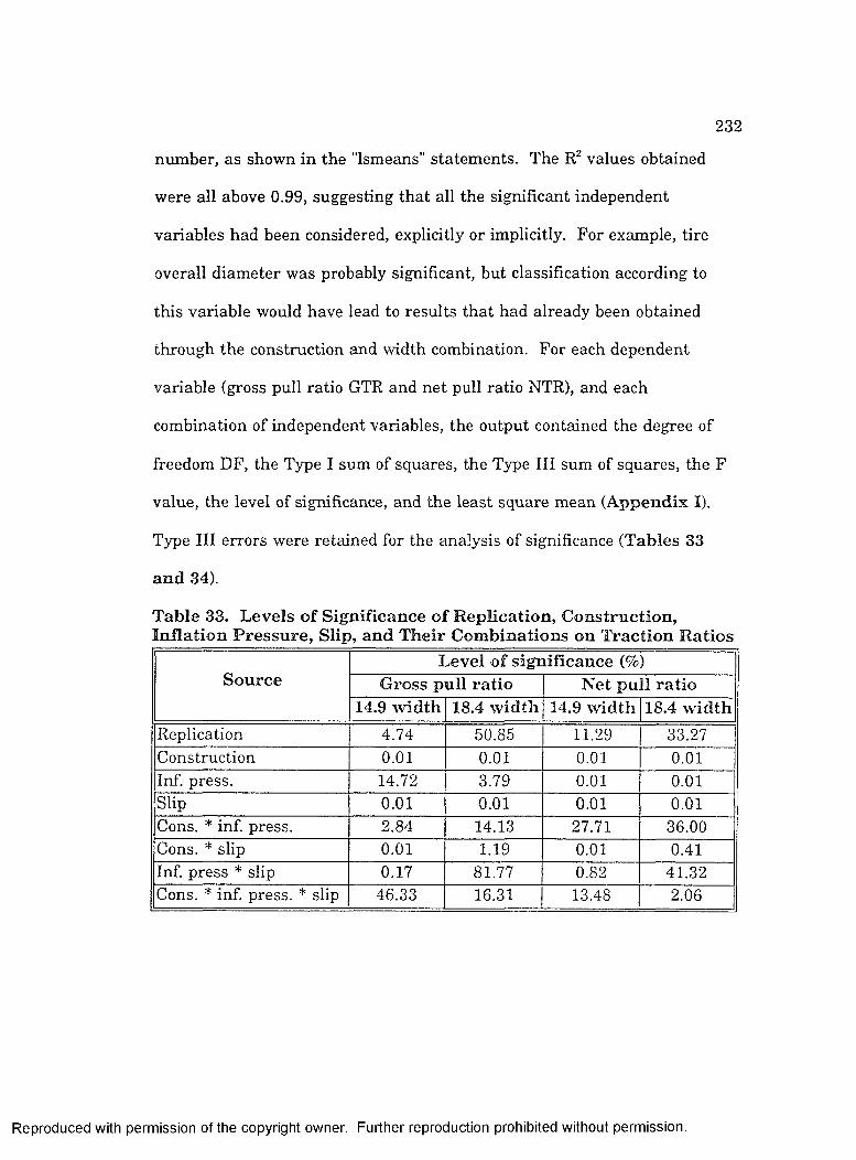
232
number, as shown in the "Ismeans" statements. The values obtained
were all above 0.99, suggesting that all the significant independent
variables had been considered, explicitly or implicitly. For example, tire
overall diameter was probably significant, but classification according to
this variable would have lead to results that had already been obtained
through the construction and width combination. For each dependent
variable (gross pull ratio GTR and net pull ratio NTR), and each
combination of independent variables, the output contained the degree of
freedom DF, the Type I sum of squares, the Type III sum of squares, the F
value, the level of significance, and the least square mean (A ppendix I).
Type III errors were retained for the analysis of significance (Tables 33
and 34).
T able 33. L evels o f S ign ifican ce o f R ep lication , C onstruction , In fla tio n P ressu re , Slip , and T heir C om binations on T raction R atios
Sou rceL evel o f s ig n ifica n ce (%)
G ross p u li ratio N et p u ll ratio14.9 w id th 18.4 w id th 14.9 w idth 18.4 w id th
Replication 4.74 50.85 11.29 33.27Construction 0.01 0.01 0.01 0.01Inf. press. 14.72 :L79 0.01 0.01Slip 0.01 0.01 0.01 0.01Cons. * inf. press. 2.84 14.13 27.71 36.00Cons. * slip 0.01 1.19 0.01 0.41Inf. press * slip 0.17 81.77 (182 41.32Cons. * inf. press. * slip 46.33 16.31 13.48 2.06
R eproduced with perm ission of the copyright owner. Further reproduction prohibited without perm ission.

233
Table 34. Levels of Significance of Replication, Tire Width, Inflation Pressure, Slip, and Their Combinations on Traction Ratios
SourceLevel of signifîcauce (%)
Gross pull ratio Net pull ratioBias-ply Radial Bias-ply Radial
Replication 69.59 0.87 64.03 3.16W idth 0.01 0.02 0.01 0.03Inf. press. 17.32 0.43 0.11 0.01Slip 0.01 0.01 0.01 0.01W idth * inf. press. - - - -W idth * slip 0.1 1.04 0.01 8T8Inf. press * slip 6.18 1.41 1.17 1.51W idth * inf. press. * slip - - - -
Replication did not appear to be highly significant, except for radial tires
(T ab le 34). This m eant th a t the results were fairly consistent, from one
replication to the other. The most significant variables were construction,
w idth and slip, which were significant a t the 1% level in all cases. Inflation
pressure was significant a t the 1% level for the net traction ratio, but not as
clearly for the gross traction ratio. The "18.4" column in T ab le 33 and the
"radial" column in T ab le 34 show a high level of significance, while the
"14.9" and "bias" columns present low levels. This suggested th a t inflation
pressure had a greater effect on net traction ratio than on gross traction
ratio. In other words, motion resistance, the difference between gross
traction and net traction, was more sensitive to inflation pressure variations
than was gross traction. Cross-effects of construction and slip, w idth and
slip, and inflation pressure and slip, had high significance levels, probably
R eproduced with perm ission of the copyright owner. Further reproduction prohibited without perm ission.

234
due to the high significance levels of slip, width and construction. The
cross-effects of slip and inflation pressure on gross traction ratio required a
closer analysis. The "14.9" column of the "GTR" p a rt of T ab le 33 and the
"bias" column of the "GTR" p a rt of T ab le 34 presented a significance level
of the cross-effect of inflation pressure and slip higher than th a t of inflation
pressure alone. The order was reversed in the "18.4" and "radial" columns.
The opposite effects of slip and inflation pressure were probably the cause of
these results: in general, the gross traction ratio tended to increase when
slip increased, or when inflation pressure decreased, bu t the combined
effects of slip and inflation pressure were confusing. Least-square means
were plotted for each tire (F ig u re s 55 to 58).
c/5z(22
<O '"CO
<J 0.3
Êk 0.2TD C rt
Ü
O .I
«---- —— »
o
------ --------------------g f -----
° ..... . .................... a ..... 0
50 ICO 150
INFLATION PRESSURE (kPa)200 250
GTR. 14.9-30 at 7.5% slip GTR, 14.9-30 at 15% slip
...Q.. NTR, 14.9-30 at 7.5% slip <> NTR, 14.9-30 at 15% slip
F igu re 55. L east-square m eans o f gi'oss pu ll ratio and n et pu ll ratio v ersu s in fla tio n p ressu re and slip for 14.9-30 tire #2.
R eproduced with perm ission of the copyright owner. Further reproduction prohibited without perm ission.

235
00Z
stua:
a00
A00<3
T3CC3
ë
0.8
0.7
0.6
OJ
0.4
0.3
0.2
0.1
^ —
A
A
---------1--------
A— »
O
O ..............o
" ■ □ .......
50 ICO 150
INFLATION PRESSURE (kPa)200 250
- 4 G TR. 14 .9R 30 al 7 .5% slip GTR, 14 .9 R 3 0 a l 15% s lip GTR. 1 4 .9 R 3 0 a i 25% slip
...Q N T R . 1 4 .9R 30 at 7 .5% slip o N T R . 14.9R 30 al 15% slip ^ N T R . 14 .9R 30 at 25% slip
F ig u re 56. L east-square m eans o f gross p u ll ra tio and n et pu ll ratio versu s in fla tio n p ressu re and slip for 14.9R30 tire #3.
0.300 Z
2tu 0.6
<O '00HCO <3
0.7
OJ
0.4
0.3
I•ac
C4HÜ
0.2
0.1
A------
« — A _______-— ^Ï---------^ -----------
O
m—O
< >
D- n . .
—--------- 1
- - ... . . .( ]
75 80 35 90 95 100
INFLATION PRESSURE (kPa)105 110 115
. G TR . 18 .4 -38 at 7.5% slip G TR . 18 .4-38 at 15% slip
N T R . 18 .4 -38 at 7.5% slip o N T R . 18 .4-38 at 15% slip
- A - G T R . 18 .4 -38 at 25% slip
A N T R. 18.4-38 at 25% slip
F ig u re 57. L east-squ are m eans o f gross p u ll ra tio and n et pu ll ratio v ersu s in fla tio n pressure and s lip for 18.4-38 tire #17.
R eproduced with perm ission of the copyright owner. Further reproduction prohibited without perm ission.
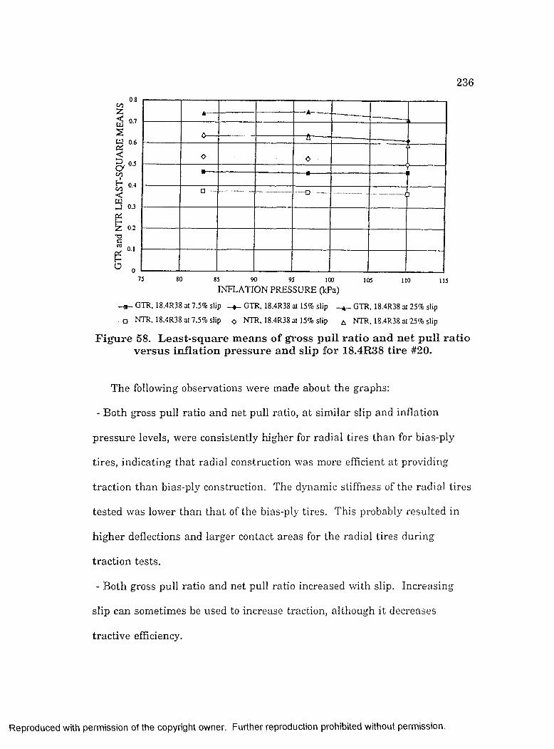
2360.8
COZ
0.7
stu 0.6o i<
OJa
A 0.400<w
0.3
1 0.2T3CC9
Ü 0
*
c--- — Ô------
o On
□.... .... ......... ]
75 80 110 11585 90 95 100 105
INFLATION PRESSURE (kPa)
G T R . 18 .4R 38 ai 7.5% slip G T R , 18.4R38 al 15% slip - a - G T R , 18.4R 38 al 25% slip
o N T R , 18 .4R 38 al 7.5% slip o N T R , 18.4R38 al 15% slip a N T R , 1 8 .4 R 3 8 a i2 5 % slip
F igu re 58. L east-square m eans o f gross p u ll ra tio and n et p u ll ratio v ersu s in fla tion p ressure and slip for 18.4R38 tire #20.
The following observations were made about the graphs:
- Both gross pull ratio and net pull ratio, a t sim ilar slip and inflation
p ressure levels, were consistently higher for radial tires than for bias-ply
tires, indicating th a t radial construction was more efficient a t providing
traction than bias-ply construction. The dynamic stiffness of the radial tires
tested was lower th an th a t of the bias-ply tires. This probably resulted in
h igher deflections and larger contact areas for the radial tires during
traction tests.
- Both gross pull ratio and net pull ratio increased with slip. Increasing
slip can sometimes be used to increase traction, although it decreases
tractive efficiency.
R eproduced with perm ission of the copyright owner. Further reproduction prohibited without perm ission.

2 3 7
- The difference between gross pull ratio and ne t pull ratio, ie. the motion
resistance ratio, increased with inflation pressure. Reducing inflation
pressure may be used to reduce energy consumption by reducing the work
required to overcome motion resistance. Because rolling radius is less
affected by dynamic load for radial tires than for bias-ply tires (T ab le 18),
travel speed of radial tires would decrease less with inflation pressure than
th a t of bias-ply tires.
- Overall, both gross pull ratio and net pull ratio tended to decrease as
inflation pressure increased. This phenomenon appeared more clearly with
n e t pull ratio th an with gross pull ratio. Thus, net pull ratio was more
sensitive than gross pull ratio to inflation pressure. However, some cases
(14.9-30 and 14.9R30 tires a t 7.5% slip) showed an increase in gross traction
ratio w ith inflation pressure. Inflation pressure reduction may be
considered a way to increase traction.
- The larger tires (18.4-38 and 18.4R38) had higher pull ratios th an the
14.9-30 and 14.9R30 tires. Because these tires have sim ilar load capacities
a t ra ted inflation pressure, the larger tires offer a clear tractive advantage.
Also, for the same load, the larger tires have a larger area of contact, due to
the ir lower inflation pressure, larger radii of curvature, and larger
deflection. This contributes to reducing contact pressure, and thus
compaction.
R eproduced with perm ission of the copyright owner. Further reproduction prohibited without perm ission.

SUMMARY AND CONCLUSIONS
Summary
A tire-loading machine was designed and bu ilt a t LSU to study
agricultural trac to r tire mechanical properties. The machine allowed the
determ ination of tire vertical stiffness under static, non-rolling conditions.
Dynamic stiffness and damping coefficient were also m easured under non
rolling conditions, by imposing a sinusoidal deflection (harmonic motion) to
the tires tested. Ten tires with sizes ranging from 14.9-30 to 18.4-38, and
representing both bias-ply and radial construction were tested. The
following observations were made;
- S tatic deflection could be satisfactorily represented as a linear function of
load.
- L inear regression analysis showed th a t both static and dynamic
stiffnesses appeared to be linearly related to inflation pressure.
- Damping coefficient tended to increase both w ith inflation pressure and
excitation frequency.
- Dynamic stiffness was not significantly affected by frequency.
- Dynamic values of stiffness were higher than static values. This
emphasized the need for dynamic m easurem ents on tires for future research
to develop vehicle dynamics models.
238
R eproduced with perm ission of the copyright owner. Further reproduction prohibited without perm ission.

239
- U nder dynamic conditions, no correlation was found betw een tire
characteristics (K^y and C^) and excitation frequency. Only general trends
were observed.
- Stiffness (static and dynamic) and dam ping coefficient varied w ith
inflation pressure, carcass construction, and tire size.
- U nder static conditions, radial tires appeared more rigid th an bias-ply
tires of the sam e size. The reverse occured under dynamic conditions.
- T ire inflation pressure variations w ith load were very small, and tire
volume changes w ith inflation pressure were also very small, suggesting
th a t changes in tire-soil contact surface area were essentially due to
geometric deform ations of the tire. The average contact pressure depended
on inflation pressure, and the contact area depended on the load to be
carried. The average contact pressure could be considered constant,
w hatever the load.
Traction experim ents done a t the National Soil Dynamics Laboratory
(NSDL, Auburn, Alabama) used four of the tires tested a t LSU (14.9-30,
14.9R30, 18.4-38 and 18.4R38). Three levels of inflation pressure (83, 138
and 207 kPa) and two levels of slip (7.5 and 15%) were investigated for the
sm aller tires, and three levels of inflation pressure (83, 97 and 110 kPa) and
th ree levels of slip (7.5, 15 and 25%) for the larger tires. The dynamic load
was increased from about 1 kN to the m aximum recommended load for the
R eproduced with perm ission of the copyright owner. Further reproduction prohibited without perm ission.

2 4 0
given inflation p ressure in each test. Known trends were verified during
the experim ents:
- R adial tires offered be tte r traction th an bias-ply tires (higher pull ratios).
This is often explained by the "track-like” behavior of radial tires, due to
th e ir reinforced belt, which m aintains a fairly constant rolling circumference
under load. The rad ial tires had lower dynamic stiffnesses th an the bias-ply
tires, and th e ir rolling radii were less sensitive to dynamic load. This
ensured larger contact areas and greater pull for the radial tires.
- Pull ratios increased w ith slip.
- L arger tires offered better traction than sm aller ones under sim ilar
conditions of load and slip. This may be explained by the larger contact
area (higher gross pull) and larger d iam eter (lower motion resistance).
- Larger tires carried the same load as the sm aller tires a t a m uch lower
inflation pressure.
O ther trends were observed during the investigation of inflation
pressure effects:
- For a given level of slip, pull ratios tended to decrease as inflation
pressure increased.
- For a given level of slip, the difference between the pull ratios, th a t is the
motion resistance ratio, increased with inflation pressure. Net pull ratio
was more sensitive than gross pull ratio to inflation pressure.
R eproduced with perm ission of the copyright owner. Further reproduction prohibited without perm ission.

2 4 1
Conclusions
- S tatic and dynamic stiffnesses proved different, although sim ilar in
trends. They cannot be used one for the other in model and sim ulation
studies. No obvious relationship was found between the two, except for the
fact th a t dynamic stiffness is generally higher, and both can be represented
as linear functions of inflation pressure.
- Tires properties under rolling conditions should be investigated more
thoroughly.
- Frequency of deformation should be accounted for in damping coefficient
models. A w ider range of excitation frequencies should be used during
fu ture experim ents to refine the observations reported here.
- Effect of rolling speed on stiffness and damping coefficient should be
investigated.
- Traction experim ents are still very complicated because m any variables
have to be considered. However, the method described here could be used
as a s tandard m ethod to provide a common base for comparisons between
tires. O ther methods often use an increasing slip, with little or no control
on actual dynamic load. Because slip and dynamic load usually rem ain
w ith in a certain range during actual field operation, both types of
experim ents p resen t advantages, w ith respect to control of the significant
variables. A common agi-eement between researchers could help define a
R eproduced with perm ission of the copyright owner. Further reproduction prohibited without perm ission.

2 4 2
standard testing procedure allowing for comparisons between resu lts
obtained in different locations.
- Soil being a determ inant factor, fu rther experiments should be m ade with
different soils, and different soil conditions (states of compaction or tillage,
"profiles" ...etc).
- The effects of hydroinflation on tire mechanical and traction properties
should be investigated.
R eproduced with perm ission of the copyright owner. Further reproduction prohibited without perm ission.

REFERENCES
Abeels, P. F. J . 1976. Tire deflection and contact studies. Jou rnal of Terram echanics 13(3):183-196. ISTVS, Hoboken, N J 07030.
Alcock, R. 1986. Tractor-Im plem ent System s. AVI Publishing Co., Inc. W estport, Connecticut.
Al-Hamed, S. A., R. D. Grisso, F. M. Zoz, and K. Von Bargen. 1990.Tractor performance spreadsheet for radial tires. ASAE P aper No. 90-1576. ASAE, S t Joseph, MI 49085.
Alim ardani, R., T. S. Colvin, and S. J. Marley. 1989. Verification of the "TERMS" traction prediction model. Transactions of the ASAE 32(3):817- 821. ASAE, S t Joseph, MI 49085.
ASAE. 1989a. ASAE Standard; ASAE S296.3. Uniform terminology for traction of agricultural tractors, self-propelled im plem ents, and other traction and transport devices. ASAE Standards 1989, pp. 118-120. ASAE, S t Joseph, MI 49085.
ASAE. 1989b. ASAE Standard: ASAE S430. A gricultural equipm ent tire loading and inflation pressures. ASAE S tandards 1989, p. 241. ASAE, S t Joseph, MI 49085.
ASAE. 1989c. ASAE Standard: ASAE EP391.1. Agricultural m achinery m anagem ent. ASAE Standards 1989, pp. 221-224. ASAE, S t Joseph, MI 49085.
ASAE. 1989d. ASAE Standard: ASAE D230.4. A gricultural m achinery m anagem ent data. ASAE Standards 1989, pp. 91-97. ASAE, St Joseph, MI 49085.
ASAE. 1989e. ASAE Standard: ASAE S430. Agricultural equipm ent tire loading and inflation pressures. ASAE Standards 1989, p. 241. ASAE, St Joseph, MI 49085.
ASAE. 1989f. ASAE Standard: ASAE 8313.2. Soil cone penetrom eter. ASAE Standards 1989, p. 517. ASAE, St Joseph, MI 49085.
Ashmore, C., E. C. Burt, and J. L. Turner. 1987. An empirical equation for predicting tractive performance of log-skidder tires. Transactions of the ASAE 30(5):1231-1236. ASAE, S t Joseph, MI 49085.
243
R eproduced with perm ission of the copyright owner. Further reproduction prohibited without perm ission.
244
Ayers, P. D., and J . Van Riper. 1991. S tress d istribution under a uniformly loaded area in agricultural soils. Transactions of the ASAE 34(3);706-710. ASAE, S t Joseph, MI 49085.
Bailey, A. C., and E. C. Burt. 1976. Theoretical considerations of a rigid wheel mechanics. Transactions of the ASAE 19(6): 1005-1007. ASAE, S t Joseph, MI 49085.
Bailey, A. C., E. C. Burt, and J . H. Taylor. 1976. Thrust-dynam ic weight relationship of rigid wheels: II. The effects of soil and wheel surface. Transactions of the ASAE 19(l):37-39. ASAE, S t Joseph, MI 49085.
Bailey, A. C., R. L. Raper, E. C. B urt, C. E. Johnson, and T. R. Way. 1992. Soil stresses under tires with low inflation pressure. ASAE Paper No. 92- 1581. ASAE, S t Joseph, MI 49085.
Baladi, G. Y., B. Rohani, and D. E. Barnes. 1984. S teerability analysis of m ultiaxle wheeled vehicles - Report 1 - Development of a soil-wheel interaction model. Technical Report GL-84-1. U.S. Army Engineer W aterways Experim ent Station, Vicksburg, M ississippi 39180.
B arnes, K. K., W. M. Carleton, H. M. Taylor, R. I. Throckmorton, and G. E. Vanden Berg. 1971. Compaction of agricultural soils. ASAE Monograph. ASAE, S t Joseph, MI 49085.
Barrelm eyer, T., K. A rm bruster, B. Langenbeck, and H. D. Kutzbach. 1993. Tyre model for vertical, longitudinal and la teral forces on driven angled tractor wheels. D epartm ent of Agricultural Engineering, U niversity of Hohenheim, Germany.
Bashford, L. L. 1985. Axle power distribution for a front-wheel assist tractor. Transactions of the ASAE 28(5): 1385-1388. ASAE, S t Joseph, MI 4 9 0 8 5 .
Bashford, L. L., G. R. Woerman, and G. J. Shropshire. 1985. Front wheel assist trac to r performance in two and four-wheel drive modes. Transactions of the ASAE 28(l):23-29. ASAE, St Joseph, MI 49085.
Bashford, L. L., S. AI-Hamed, and C. Jenane. 1992. Effects of tire size and pressure on tractive performance. ASAE Paper No. 92-1011. ASAE, S t Joseph, MI 4 9 0 8 5 .
R eproduced with perm ission of the copyright owner. Further reproduction prohibited without perm ission.

2 4 5
Bashford, L. L., S. Al-Hamed, and C. Jenane. 1993. Effects of tire size and inflation pressure on tractive performance. Applied Engineering in A griculture 9(4):343-348. ASAE, S t Joseph, MI 49085.
Bekker, M. G. 1956. Theory of Land Locomotion - The Mechanics of Vehicle M obiltiv. University of Michigan Press, Ann Arbor, Michigan.
Bekker, M. G. 1960. OfF-the-Road Locomotion. Research and Development in Terram echanics. The University of Michigan Press. Ann Arbor, M ichigan.
Bekker, M. G. 1969. Introduction to Terrain-Vehicle System s. The U niversity of Michigan Press. Ann Arbor, Michigan.
Billington, W. P. 1973. The N.I.A.E. Mk II single wheel tester. Journal of A gricultural Engineering Research 18(l):67-70. NIAE, Silsoe, England.
Blaszkiewicz, Z. 1990. A m ethod for the determ ination of the contact area between a tyre and the ground. Journal of Terram echanics 27(4):263-282. ISTVS, Hoboken, N J 07030.
Block, W. A., E. C. B urt, and C. E. Johnson. 1989. Computer graphics sim ulation of tire lug interfacing with soil. ASAE P aper No. 89-1560.ASAE, S t Joseph, MI 49085.
Block, W. A., R. L. Raper, C. E. Johnson, E. C. B urt, and A. C. Bailey.1990a. Comparison of soil stress sta te predictions for rigid wheel. ASAE Paper No. 90-1547. ASAE, St Joseph, MI 49085.
Block, W. A., C. E. Johnson, E. C. B urt, A. C. Bailey, and R. L. Raper.1990b. Graphical anim ation depicting stress under a rigid wheel. ASAE Paper No. 90-1091. ASAE, St Joseph, MI 49085.
B rassart, F. 1989. A computer system to select agricultural tractor tires. U npublished M.S. Thesis, Louisiana S tate University, Baton Rouge, LA 70803.
Brixius, W. W., and R. D. Wismer. 1978. The role of Slip in Traction.ASAE P aper No. 78-1538. ASAE, S t Joseph, MI 49085.
Brixius, W. W. 1987. Traction prediction equations for bias-ply tires.ASAE P aper No. 87-1622. ASAE, S t Joseph, MI 49085.
R eproduced with perm ission of the copyright owner. Further reproduction prohibited without perm ission.

2 4 6
Buckingham, F. 1985a. U nderstanding those N ebraska Tests - W hat are the tests? How are they used? Im plem ent and Tractor 100(l):8-20. In tertec Publishing Corp., Overland Park, KS 66215.
Buckingham , F. 1985b. Using N ebraska Tests to select a tractor. Im plem ent and Tractor 100(6):36-43. In tertec Publishing Corp., Overland Park , KS 66215.
B urt, E. C., and R. L. Schafer. 1972. New technique for m easuring tangential stresses a t the soil-wheel interface of a rigid wheel. Transactions of the ASAE 15(4):613-614,619. ASAE, S t Joseph, MI 49085.
B urt, E. C., and A. C. Bailey. 1975. Thrust-dynam ic weight relationship of rigid wheels. Transactions of the ASAE 18(5):811-813,817. ASAE, St Joseph, MI 49085.
B urt, E. C., C. A. Reaves, A. C. Bailey, and W. D. Pickering. 1980. A machine for testing tractor tires in soil bins. Transactions of the ASAE 23(3);546-547, 552. ASAE, S t Joseph, MI 49085.
B urt, E. C., and A. C. Bailey. 1982. Load and inflation pressure effects on tires. Transactions of the ASAE 25(4):881-884. ASAE, S t Joseph, MI 49085.
B urt, E. C., P. W. L. Lyne, P. Meiring, and J. F. Keen. 1983. B allast and inflation effects on tire efficiency. Transactions of the ASAE 26(5); 1352- 1354. ASAE, S t Joseph, MI 49085.
B urt, E. C., and P. W. L. Lyne. 1985. Velocity effects on traction performance. Transactions of the ASAE 28(6):1729-1730. ASAE, S t Joseph, MI 49085.
B urt, E. C., R. K. Wood, and A. C. Bailey. 1989. Dynamic load effects on the tangential-to-norm al stress ratio for pneum atic tires. Transaction of the ASAE 32(4):1177-1181. ASAE, St Joseph, MI 49085.
B urt, E. C., R. K. Wood, and A. C. Bailey. 1990. Some comparisons of average to peak soil-tire contact pressures. ASAE Paper No. 90-1094.ASAE, S t Joseph, MI 49085.
B urt, E. C., R. K. Wood, and A. C. Bailey. 1992. Some comparisons of average to peak soil-tire contact pressures. Transactions of the ASAE 35(2):401-404. ASAE, S t Joseph, MI 49085.
R eproduced with perm ission of the copyright owner. Further reproduction prohibited without perm ission.

2 4 7
Campbell, W. P., and S. D. Parsons. 1992. Power to weight ratio m easurem ents on Ind iana farm tractors. ASAE Paper No. 92-1045. ASAE, S t Joseph, MI 49085.
C arpenter, T. G., N. R. Fausey, and R. C. Reeder. 1985. Theoretical effect of wheel loads on subsoil stresses. Soil and Tillage Research 6(2): 179-192. Elsevier Scientific Publishing Company, Am sterdam , The N etherlands.
Chancellor, W. J . 1977. Compaction of soil by agricultural equipm ent - B ulletin 1881. Division of Agricultural Sciences, University of California, Berkeley, CA 94720.
Chang, C. S., and A. W. Cooper. 1969. A study of the mechanics of tractor wheels. Transactions of the ASAE 12(3):384-388. ASAE, S t Joseph, MI 49085.
Charles, S. M., and D. J . Schuring. 1984. An empirical model for predicting the effective rolling radius of agricultural drive tires. ASAE P aper No. 84-1555. ASAE, S t Joseph, MI 49085.
Chung, T. J ., and J. K. Lee. 1975. Dynamics of viscoelastoplastic soil under a moving wheel. Journal of Terram echanics 12(1):15-31. ISTVS, Hoboken, N J 07030.
Clark, S. K. 1981. Mechanics of Pneum atic T ires. U.S. D epartm ent of T ransportation. N ational Highway Traffic Safety Adm inistration, W ashington, D. C. 20590.
Clark, R. L. 1985. Tractive modeling w ith the modified W ism er-Luth model. ASAE Paper No. 85-1049. ASAE, St Joseph, MI 49085.
Coleman, G. E. Ill, and J. V. Perum pral. 1974. The finite elem ent analysis of soil compaction. Transactions of the ASAE 17(5):856-860. ASAE, St Joseph, MI 49085.
Collins, T. S. 1991. Loads in tractor linkages when transporting rear m ounted im plem ents - Development of modelling and m easurem ent techniques. Journal of Agricultural Engineering Research 49(3):165-188. NIAE, Silsoe, England.
Collet, M. 1988. Pression des pneum atiques arrière: le réglage à la dem ande mis au point par Massey-Ferguson. Bulletin Technique du M achinisme et de l’Equipem ent Agricoles No. 25, pp. 4-5, CEMAGREF, Antony, France.
R eproduced with perm ission of the copyright owner. Further reproduction prohibited without perm ission.

248
Crolla, D. A., D. N. L. Horton, and R. M. Stayner. 1990. Effect of tyre modelling on trac to r ride vibration predictions. Journal of Agricultural Engineering Research 47(l);55-77. NIAE, Silsoe, England.
Czako, T. F. 1974. The influence of inflation pressure on cross-country perform ance. Journal of Terram echanics 11(3&4): 13-23. ISTVS, Hoboken, N J 07030.
Dagan, G., and M. P. Tulin. 1969. A study of the steady flow of a rigid- plastic clay beneath a driven wheel. Journal of Terram echanics 6(2):9-27. ISTVS, Hoboken, N J 07030.
Das, B. M. 1983. Advanced Soil M echanics. McGraw Hill, New York.
De Souza, E. G., and L. F. Milanez. 1991. Prediction of tracto r perform ance on concrete (Corrected). Transactions of the ASAE 34(3):727- 732. ASAE, S t Joseph, MI 49085.
De Souza, E., N. J . F. Pinho, and L. F. Milanez. 1991. B allast optimization of a front wheel assis t tractor. ASAE Paper No. 91-1593. ASAE, S t Joseph, MI 49085.
Domier, K. W. 1978. Traction analysis of N ebraska Tractor Tests. Transactions of the ASAE 21(2):244-248. ASAE, St Joseph, MI 49085.
Downs, H. W., R. K. Taylor, and A. Al-Janobi. 1990. A decision aid for optimizing tractor-im plem ent systems. ASAE Paper No. 90-1569. ASAE, St Joseph, MI 49085.
Dwyer, M. J., D. R. Comely, and D. W. Evernden. 1974. The field perform ance of some trac to r tyres related to soil mechanical properties. Journal of Agricultural Engineering Research 19(l);35-50. NIAE, Silsoe, England.
Dwyer, M. J., D. W. Evernden and M. McAllister. 1976. Handbook of agricultural tyre performance. Report No. 18. NIAE, Silsoe, England.
Dwyer, M. J., D. W. Evernden and M. McAllister. 1977. Comparison of the tractive perform ance of a tractor driving wheel during its first and second passes in the same track. Journal of Terram echanics 14(1): 1-10. ISTVS, Hoboken, N J 07030.
R eproduced with perm ission of the copyright owner. Further reproduction prohibited without perm ission.
2 4 9
Dwyer, M. J . 1978. M aximising agricultural tractor perform ance by m atching weight, ty re size and speed to the power available. Proceedings of the Sixth In ternational Conference of ISTVS. ISTVS, Hoboken, N J 07030.
Dwyer, M. J . 1984. The tractive performance of wheeled vehicles. Journal of Terram echanics 21(1): 19-34. ISTVS, Hoboken, N J 07030.
Dwyer, M. J., and D. P. Heigho. 1984. The tractive perform ance of some large trac to r drive wheel tyres compared w ith dual wheels. Journal of A gricultural Engineering Research 29(3):43-50. NIAE, Silsoe, England.
Ellis, R. W. 1977. T ractor design requirem ents and selection considerations. T ractor Design No. 3. ASaAE distinguished lecture series. ASAE, S t Joseph, MI 49085.
Em swiler, J . E., and F. L. Schwartz. 1943. Thermodynamics (5‘*’ Edition). McGraw-Hill, New York.
E rad a t Oskoui, K., B. D. Witney, and W. B. Voorhees. 1990. A knowledge- based m achinery m anagem ent system. ASAE P aper No. 90-7059. ASAE, St Joseph, MI 49085.
Erbach, D. C., and K. K. Knoll. 1992. Inflation pressure effect on soil compaction. ASAE P aper No. 92-1582. ASAE, S t Joseph, MI 49085.
Erickson, L. R., and W. E. Larsen. 1983. Four wheel drive tracto r field performance. Transactions of the ASAE 26(5):1346-1351. ASAE, S t Joseph, MI 49085.
The European Tyre and Rim Technical O rganisation (ETRTO). 1993. S tandards M anual. ETRTO, Brussels, Belgium.
Evans, M. D., R. L. C lark, and G. Manor. 1989. A traction prediction and ballast selection model. ASAE Paper No. 89-1054. ASAE, S t Joseph, MI 4 9 0 8 5 .
Evans, M. D., R. L. C lark, and G. Manor. 1991. An improved traction model for b a llast selection. Transactions of the ASAE 34(3);773-780. ASAE, S t Joseph, MI 49085.
Feda, J. 1978. S tress in Subsoil and Methods of Final Settlem ent Calculation - Developments in Geotechnical Engineering 18. Elsevier Scientific Publishing Company, New York 10017.
R eproduced with perm ission of the copyright owner. Further reproduction prohibited without perm ission.

2 5 0
Firestone Agribusiness. 1991a. Field power hop on mechanical front wheel drive tractors. Agribusiness Technical Bulletin F-Oll-X. Firestone Agribusiness, Des Moines, Iowa 50309.
Firestone Agribusiness. 1991b. Tractor tires field power hop on four wheel drive tractors. Agribusiness Technical Bulletin F-035-X. Firestone Agribusiness, Des Moines, Iowa 50309.
Freeland, R. S., F. D. Tompkins, L. R. Wilhelm, and J. R. Sarten. 1990. Instrum enta tion for m easuring tractor chassis acceleration. ASAE Paper No. 90-1012. ASAE, S t Joseph, MI 49085.
Freitag, D. R. 1966. A dimensional analysis of the performance of pneum atic tires on clay. Journal of Terram echanics 3(3):51-68. ISTVS, Hoboken, N J 07030.
Freitag, D. R. 1990. Discussion - Sources of variability in traction data. Journal of Terram echanics 27(2):159. ISTVS, Hoboken, N J 07030.
Frohlich, 0 . K. 1934. Druckverteilung im Baugrunde, m it besonderer Berücksichtigung der plastischen Erscheinungen. Springer Verlag, Vienna.
Fujimoto, Y. 1977. Performance of elastic wheels on yielding cohesive soils. Journal of Terram echanics 14(4):191-210. ISTVS, Hoboken, N J 07030.
G assm an, P. W., D. C. Erbach, and S. W. Melvin. 1989. Analysis of track and wheel soil compaction. Transactions of the ASAE 32(l):23-29. ASAE,S t Joseph, MI 49085.
Gee-Clough, D., M. McAllister, G. Pearson, and D. W. Evernden. 1978. The empirical prediction of tractor-im plem ent field performance. Journal of Terram echanics 15(2);81-94. ISTVS, Hoboken, N J 07030.
Gee-Clough, D. 1980. Selection of tyre sizes for agricultural vehicles. Journal of A gricultural Engineering Research 25(3):261-278. NLAE, Silsoe, England.
Gee-Clough, D., G. Pearson, and M. McAllister. 1982. Ballasting wheeled tractors to achieve maximum power output in frictional-cohesive soils. Journal of A gricultural Engineering Research 27(1):1-19. NIAE, Silsoe, England.
Gill, W. R., and G. E. Vanden Berg. 1968. Soil Dynamics in Tillage and T raction. USD A Agricultural Handbook No. 316. United States
R eproduced with perm ission of the copyright owner. Further reproduction prohibited without perm ission.

2 5 1
Governm ent P rin ting Office, W ashington, D.C. Agricultural Research Service, USDA, 511 p.
Gill, W. R. 1990. The National Soil Dynamics Laboratory, U nited S tates D epartm ent of Agriculture, Agricultural Research Service - In ternational Historic M echanical Engineering Landm ark and Historic Landm ark of A gricultural Engineering. ASME/ASAE HH0990. ASAE, S t Joseph, MI 49085.
The Goodyear Tire and Rubber Company. 1984. Farm Tire Hanbook. Goodyear, Farm Tire Sales D epartm ent, Akron, OH 44316.
The Goodyear Tire and Rubber Company. 1992. Optimum tractor tire perform ance handbook. The Goodyear Tire and Rubber Company, Akron, OH 44316.
The Goodyear Tire and Rubber Company. 1994. Farm Tire Hanbook. Goodyear, F arm Tire Sales D epartm ent, Akron, OH 44316.
Goupillon, J . F., and E. Hugo. 1988. M esure de la puissance aux essieux des tracteurs - Objectifs et méthodes (M easurem ent of tractor horsepower on the axles - Objectives and methods). Bulletin Technique du M achinisme et de l’Equipem ent Agricoles No. 32, CEMAGREF, Antony, France.
Greenlee, J . G., J . D. Summers, and K. P. Self. 1986. Effect of velocity on tractive performance of tractor tires. ASAE Paper No. 86-1539. ASAE, St Joseph, MI 49085.
Grisso, R. D., R. K. Taylor, T. R. Way, and L. L. Bashford. 1991. Tractive performance of 18.4R46 and 18.4R42 radial tractor tires. ASAE Paper No. 91-1589. ASAE, St Joseph, MI 49085.
Grisso, R. D., R. K. Taylor, T. R. Way, and L. L. Bashford. 1992a. Tractive performance of 18.4R46 and 18.4R42 radial tractor tires. Applied Engineering in Agriculture 8(6);739-745. ASAE, S t Joseph, MI 49085.
Grisso, R. D., S. A. Al-Hamed, R. K. Taylor, and F. M. Zoz. 1992b. D em onstrating tractor performance trends using Lotus tem plates. Applied Engineering in Agricultural 8(6);733-738. ASAE, St Joseph, MI 49085.
Gu, Y., and R. L. Kushwaha. 1992. Dynamic load distribution and tractive performance of a model tractor. ASAE Paper No. 92-1018. ASAE, S t Joseph, MI 49085.
R eproduced with perm ission of the copyright owner. Further reproduction prohibited without perm ission.

252
Guo, H., and R. Schuler. 1992. Num erical sim ulation of wheel induced soil compaction. ASAE P aper No. 92-1053. ASAE, St Joseph, MI 49085.
H arris, H. D., and F. Pearce. 1990. A universal m athem atical model of diesel engine performance. Journal of Agricultural Engineering Research, 47(3):165-176. NIAE, Silsoe, England.
H arris, H. D. 1992a. Prediction of torque and optimum operating po in t of diesel engines using engine speed and fuel consumption. Jou rna l of A gricultural Engineering Research, 53(2):93-101. NIAE, Silsoe, England.
H arris, H. D. 1992b. Prediction of trac to r engine perform ance using OECD standard test data. Journal of A gricultural Engineering Research, 53(3):181-193. NIAE, Silsoe, England.
Howson, D. P., and N. Y. Williams. 1961. Traction surface for a treadm ill for testing pneum atic-tyred tractors. Research Note. Journal of A gricultural Engineering Research 6(3):217-220. NIAE, Silsoe, England.
Howson, D. F. 1963. Development of a treadm ill for testing pneum atic- tyred tractors. Journal of Agricultural Engineering Research 8(1):88-91. NIAE, Silsoe, England.
Howson, D. F., and N. Y. Williams. 1963. Limited differential w heelslip control on the N.I.A.E. hydrostatic tractor. Journal of A gricultural Engineering Research 8(2):185-193. NIAE, Silsoe, England.
Iff, R. H., J. L. Roger, E. C. B urt, and E. W. Culver. 1984. C-A-R-T-S; Capacity analysis of rubber-tired skidders. Transactions of the ASAE 27(3):660-664. ASAE, S t Joseph, Ml 49085.
Jah n s, G., K. J . Forster, and M. Hellickson. 1990. Com puter sim ulation of diesel engine performance. Transactions of the ASAE 33(3):764-770. ASAE, S t Joseph, Ml 49085.
Janosi, Z. 1960. Soil values in land locomotion. Journal of A gricultural Engineering Research 5(l);19-27. NIAE, Silsoe, England.
Janssen , M. L., and D. J . Schuring. 1985. S tructural and perform ance characteristics of agricultural tires. ASAE/SAE Paper No. 85-1090. ASAE, S t Joseph, Ml 49085.
R eproduced with perm ission of the copyright owner. Further reproduction prohibited without perm ission.

2 5 3
Johnson, C. E., and E. C. B urt. 1990. A m ethod of predicting soil stress s ta te under tires. Transactions of the ASAE 33(3):713-717. ASAE, S t Joseph, MI 49085.
Johnson, C. E., A. C. Bailey, and E. Cakir. 1992. U nderstanding soil response to m ultiple loading. ASAE P aper No. 92-1051. ASAE, S t Joseph, MI 49085.
Khalid, M., and J . L. Sm ith. 1981. Axle torque distributions in 4WD tractors. Journal of Terram echanics 18(3):157-167. ISTVS, Hoboken, N J 07030.
Khamidov, A. 1961. Use of gam m a-rays in the study of the effects of wheels on the soil (T ranslated from Russian). Jou rna l of A gricultural Engineering Research 6(2):147-152. NIAE, Silsoe, England.
Rising, A., and H. Gohlich. 1989. Dynamic characteristics of large tires. Journal of A gricultural Engineering Research 43(1):11-21. NIAE, Silsoe, England.
Kolozsi, Z., and T. T. M cCarthy. 1974. The prediction of tracto r field performance. Journal of Agricultural Engineering Research 19(2):167-172. NIAE, Silsoe, England.
Komandi, G. 1976. The determ ination of the deflection, contact area, dimensions, and load carrying capacity for driven pneum atic tires operating on concrete pavem ent. Journal of Terram echanics 13(1): 15-20. IS W S , Hoboken, N J 07030.
Koolen, A. J ., and H. Kuipers. 1983. Agricultural Soil Mechanics - Advanced Series in Agricultural Sciences 13. Springer-Verlag, Berlin, Germany.
Kotzabassis, C., B. A. Stout, S. W. Searcy, and G. Felsenstein. 1987. Validation of an in-soil tracto r performance prediction model. ASAE Paper No. 87-1023. ASAE, S t Joseph, MI 49085.
Kotzabassis, C., and B. A. Stout. 1989. Tractor-im plem ent in teraction model. ASAE Paper No. 89-1025. ASAE, S t Joseph, MI 49085.
Kotzabassis, C., B. A. Stout, and D. W hittaker. 1989. A Prolog tractor- im plem ent m atching expert system. ASAE Paper No. 89-7080. ASAE, St Joseph, MI 49085.
R eproduced with perm ission of the copyright owner. Further reproduction prohibited without perm ission.

2 5 4
Kravig, K. K. 1986. Factors tha t affect the perform ance and efficiency of 4WD tractors. ASAE Paper No. 86-1547. ASAE, S t Joseph, MI 49085.
Krick, G. 1969. Radial and shear stress distribution under rigid wheels and pneum atic tires operating on yielding soils w ith consideration of tire deformation. Jou rna l of Terramechanics 6(3);73-98. ISTVS, Hoboken, N J 07030.
Laib, L. 1979. On the dynamic behavior of agricultural tires. Journal of Terram echanics 16(2);77-85. ISTVS, Hoboken, N J 07030.
Leviticus, L. I. 1985. Tractive efficiency and power-weight ratio tables. N ebraska Tractor Test Laboratory, University of N ebraska, Lincoln, NE 68583.
Leviticus, L. I., and J. F. Reyes. 1985. Tractor perform ance on concrete. Transactions of the ASAE 28(5):1425-1429. ASAE, S t Joseph, MI 49085.
Lima, J. S. S., E. G. Souza, and L. F. Milanez. 1992. Overall efficiency of a tracto r in field. ASAE Paper No. 92-1517. ASAE, S t Joseph, MI 49085.
Lines, J. A., and N. A. Young. 1989. A machine for m easuring the suspension characteristics of agricultural t>Tes. Journal of Terram echanics 26(3 & 4):201-210. ISTVS, Hoboken, N J 07030.
Lines, J. A., and K. Murphy. 1991. The stiffness of agricultural tractor tires. Journal of Terram echanics 28(l):49-64. ISTVS, Hoboken, N J 07030.
Lopp, L. C. 1992. Optim um tractor tire performance. ASAE Paper No. 92- 1787. ASAE, S t Joseph, MI 49085.
Lyne, P. W. L., E. C. B urt, and J. D. Jarrel. 1983. Com puter control for the NMTL single-wheel tester. ASAE Paper No. 83-1555. ASAE, St Joseph, MI 49085.
Macnab, J . E., R. B. W ensink, and D. E. Booster. 1977. Modeling wheel tracto r energy requirem ents and tractive performances. Transactions of the ASAE 20(41:602-605, 609.
M arquez, L. 1980. Prediccion del comportamiento de un tractor a la barra a p a rtir del ensayo de su motor en banco (Prediction of the draw bar behavior of a trac to r from its engine bench tests). Doctoral Dissertation. U niversidad Polytechnica de Madrid, Escuela Técnica Superior de Ingenieros Agronomes, M adrid, Spain.
R eproduced with perm ission of the copyright owner. Further reproduction prohibited without perm ission.

255
McDonald, T. P., B. J. Stokes, and J. Wilhoit. 1992. Field evaluation of skidder tire tractive performance. ASAE Paper No. 92-7514. ASAE, St Joseph, MI 49085.
McDonald, T. P., B. J. Stokes, and J . Wilhoit. 1993. Field evaluation of skidder tire tractive performance. Applied Engineering in Agriculture 9(6):571-576. ASAE, S t Joseph, MI 49085.
McKibben, E. G., and R. L. Green. 1940. T ransport wheels for agricultural m achines - VII -Relative effects of steel wheels and pneum atic tires on agricultural soil. Agricultural Engineering 21(5);183-185. ASAE, S t Joseph, MI 49085.
McKyes, E. 1985. Soil C utting and Tillage - Developments in agricultural engineering 7 . Elsevier Scientific Publishing Company, New York, NY 10017.
Michelin Tire Company. 1988. Pneus agricoles, forestiers, industriels - Inform ations teclmiques (Agricultural, forestry and industrial tires - Technical information). Michelin Tire Company, C lerm ont-Ferrand, France.
Murillo-Soto, F., and J. L. Smith. 1977. W eight transfer in 4WD tractors:A model study. Transactions of the ASAE 20(2):253-257. ASAE, S t Joseph, MI 49085.
Murillo-Soto, F., and J. L. Smith. 1978. Traction efficiency of 4WD tractors: A model study. Transactions of the ASAE 21(6):1051-1053. ASAE, S t Joseph, MI 49085.
M urphy, N. R., and A. J. Green. 1969. Effects of test techniques on wheel performance. Journal of Terramechanics 6(l):37-62. ISTVS, Hoboken, NJ 07030.
Mussel, U., I. Shmulevich, and D. Wolf. 1992. The effect of dynamically varying velocity on wheel traction. ASAE Paper No. 92-1013. ASAE, St Joseph, MI 49085.
N ation, H. J ., and M. W. Jesson. 1957. A load vehicle for tractor testing. Journal of Agricultural Engineering Research 2(1):1-11. NIAE, Silsoe, England.
Nowatzki, E. A., and L. L. Karafiath. 1974. General yield conditions in a plasticity analysis of soil-wheel interaction. Journal of Terram echanics ll(l):29-44 . ISTVS, Hoboken, N J 07030.
R eproduced with perm ission of the copyright owner. Further reproduction prohibited without perm ission.

2 5 6
Okello, J . A. 1991. A review of soil strength m easurem ent techniques for prediction of te rra in vehicle performance. Journal of Agricultural Engineering Research 50(2):129-155. NIAE, Silsoe, England.
Okello, J . A. 1992. Prediction of the force distribution between the soil and a pneum atic wheel. Journal of Agricultural Engineering Research 51(4):249-262. NIAE, Silsoe, England.
O rganization for Economic Cooperation and Development (OECD). 1984. OECD tandard codes for the testing of agricultural tractors and protective structures. Predicting tractor field perform ance from test data. Ref. AGR/TS(84)9, Paris, France.
Osm an, M. S. 1964. The m easurem ent of soil shear strength. Journal of Terram echanics l(3):54-60. ISTVS, Hoboken, N J 07030.
P ain ter, D. J. 1981. A simple deflection model for agricultural trac to r tires. Jou rnal of A gricultural Engineering Research 26(l);9-20. NIAE, Silsoe, England.
Perdok, U. D. 1978. A prediction model for the selection of tyres for towed vehicles on tilled soil. Journal of Agricultural Engineering Research 23(4);369-383. NIAE, Silsoe, England.
Persson, S. P. E. 1967a. Param eters for tracto r wheel performance - P a r t I: Definitions. Transactions of the ASAE 10(3):420-423. ASAE, S t Joseph, MI 49085.
Persson, S. P. E. 1967b. Param eters for tracto r wheel performance - P a rt II: Description and use. Transactions of the ASAE 10(3):424-426. ASAE, St Joseph, MI 49085.
Persson, S. 1991. Tractive power ratio useful for describing traction device performance. ASAE Paper No. 91-1588. ASAE, S t Joseph, MI 49085.
Perum pral, J . V., J . B. Liljedahl, and W. H. Perloff. 1971. The finite elem ent m ethod for predicting stress distribution and soil deformation under a tractive device. Transactions of the ASAE 14(6):1184-1188. ASAE, St Joseph, MI 49085.
Peters, B. L. 1983. Weight transfer analysis on four-wheel drive tractors. ASAE P aper No. 83-1068. ASAE, S t Joseph, MI 49085.
R eproduced with perm ission of the copyright owner. Further reproduction prohibited without perm ission.

2 5 7
Phillips, J . R. 1961. The powered vehicular wheel plane-rolling in equilibrium : A consideration of slip and rolling resistance. Proceeding No. 34 of the F irs t In ternational Conference on the Mechanics of Soil-Vehicle System s, Turin, Italy, pp. 541-557. ISTVS, Hoboken, New Jersey 07030.
Pigg, C. 1990. Incorrect ballasting lowers performance. Im plem ent and Tractor, May 1990, p. 12. Intertec Publishing Corp., Overland Park , KS 66215.
P itts , M. J., and C. E. Goering. 1979. Modeling soil cone index changes induced by drive wheel traffic. ASAE Paper No. 79-1552. ASAE, S t Joseph, MI 49085.
P lackett, C. W. 1984. The ground pressure of some agricultural tyres a t low load and w ith zero sinkage. Journal of Agricultural Engineering R esearch 29(2): 159-166. NIAE, Silsoe, England.
P lackett, C. W. 1985. Review of force prediction methods for off-road wheels. Journal of A gricultural Engineering Research 31(l):l-29. NIAE, Silsoe, England.
Plouffe, C., S. Tessier, D. Angers, and L. Chi. 1991. A McIntosh based soil compaction teaching aid. ASAE Paper No. 91-5515. ASAE, St Joseph, MI 49085.
Pope, R. G. 1969. The effect of sinkage ra te on pressure sinkage relationships and rolling resistance in real and artificial clays. Journal of Terram echanics 6(4):31-38. ISTVS, Hoboken, N J 07030.
Pope, R. G. 1971. The effect of wheel speed on rolling resistance. Journal of Terram echanics 8(l):51-58. ISTVS, Hoboken, N J 07030.
Rackham , D. H., and D. P. Blight. 1985. Four-wheel drive tractors - A review. Journal of Agricultural Engineering Research 31(3);185-201. NIAE, Silsoe, England.
Ramp, D. P., and J. C. Siemens. 1990. Tractor/im plem ent m atching for perform ance and productivity. ASAE Paper No. 90-1562. ASAE, S t Joseph, MI 49085.
Rao, S. S. 1990. Mechanical V ibrations. 2"‘‘ Edition. Addison-Wesley Publishing Company, Reading, M assachusetts.
R eproduced with perm ission of the copyright owner. Further reproduction prohibited without perm ission.

258
Raper, R. L., and D. C. Erbach. 1990a. Effect of variable linear elastic param eters on finite elem ent prediction of soil compaction. Transactions of the ASAE 33(3):731-736. ASAE, S t Joseph, MI 49085.
Raper, R. L., and D. C. Erbach. 1990b. Prediction of soil stresses using the finite elem ent method. Transactions of the ASAE 33(3):725-730. ASAE, St Joseph, MI 49085.
Raper, R. L., A. C. Bailey, E. C. B urt, and C. E. Johnson. 1991. An in tegrated approach using tire and soil stresses to predict soil compaction. ASAE Paper No. 91-1823. ASAE, S t Joseph, MI 49085.
Raper, R. L., A. C. Bailey, E. C. B urt, T. R. Way, and P. L iberati. 1993. Inflation pressure and dynamic load effects on soil deformation and soil-tire interface stresses. ASAE Paper No. 93-1517. ASAE, S t Joseph, MI 49085.
Reyes, A., R. B. Dodd, and T. H. G arner. 1989. Non linear finite elem ent program for soil compaction. ASAE Paper No. 89-3530. ASAE, S t Joseph, MI 49085.
Rode, R., Pirelli-Arm strong Tire Company. 1989. Personnal communications.
Rousselet, M. 1988. T ransport en agriculture et remorques agraires - Les essieux et les pneum atiques (Agricultural transports and wagons - Axles and pneum atic tires). Bulletin Technique du Machinisme et de l’Equipem ent Agricoles 30:37-40. CEMAGREF, Antony, France.
Rum m er, R. B. 1989. Com puter sim ulation of ride dynamics for the design of forest machines. Transactions of the ASAE 32(1):12-16. ASAE, St Joseph, MI 49085.
Schuring, D. 1964. The mechanics of rigid wheels on soft ground. Journal of Terram echanics 1(2):5-21. ISTVS, Hoboken, N J 07030.
Self, K. P., J . D. Sum m ers, J. G. Greenlee, and G. L. McLaughlin. 1986. A mobile off-road tire test apparatus. ASAE Paper No. 86-1538. ASAE, St Joseph, MI 49085.
Siefkes, T., and H. Gohlich. 199?. Dynamic characteristics of vei*y large tires. Technical University of Berlin, Institu te of Agricultural Engineering, Berlin, Germany.
R eproduced with perm ission of the copyright owner. Further reproduction prohibited without perm ission.

2 5 9
Soane, B. D., P. S. Blackwell, J. W. Dickson, and D, J . P ain ter. 1981a. Compaction by agricultural vehicles: A review - I - Soil and wheel characteristics. Soil and Tillage Research l(3):207-237. Elsevier Scientific Publishing Company, Am sterdam , The N etherlands.
Soane, B. D., P. S. Blackwell, J. W. Dickson, and D. J. Pain ter. 1981b. Compaction by agricultural vehicles: A review - II - Compaction under tyres and other runn ing gear. Soil and Tillage Research l(4):373-400. E lsevier Scientific Publishing Company, Amsterdam, The N etherlands.
Soehne, W. 1958. Fundam entals of pressure distribution and soil compaction under tractor tires. Agricultural Engineering 39(5):276-291. ASAE, S t Joseph, MI 49085.
Sohne, W. 1968. Four-wheel drive or reai*-wheel drive for high power farm tractors. Journal of Terram echanics 5(3):9-28. ISTVS, Hoboken, N J 07030.
Song, A., B. K. Huang, and H. D. Bowen. 1989. Sim ulating a powered model w heel-tractor on soft ground. Transactions of the ASAE 32(1X2-11. ASAE, S t Joseph, MI 49085.
Sonnen, F. J . 1969. Drawbar performance of high-powered farm tractors w ith rear-wheel and four-wheel drive. Journal of Terram echanics 6(1):7-21. ISTVS, Hoboken, N J 07030.
Stafford, J . V., and P. de Carvalho Mattos. 1981. The effect of forward speed on wheel-induced soil compaction: Laboratory sim ulation and field experiments. Journal of Agricultural Engineering Research 26(4):333-347. NIAE, Silsoe, England.
Successful Farm ing. 1986. Farm Tire Handbook II. Successful Farm ing, Des Moines, lA 50336.
Successful Farm ing. 1988. Farm Tire Handbook III. Successful Farm ing, Des Moines, lA 50336.
Sum m ers, J . D., and K. Von Bargen. 1983. A simplified tractor performance sim ulation model. ASAE Paper NO. 83-1564. ASAE, St Joseph, MI 49085.
Sum m ers, J . D., R. E. Ekstrom , K. Von Bargen. 1986. Development of a tractor performance sim ulation model. Transactions of the ASAE 29(3):661- 666 . ASAE, S t Joseph, MI 49085.
R eproduced with perm ission of the copyright owner. Further reproduction prohibited without perm ission.

2 6 0
Tanaka, T. 1961. The statical analysis and experim ent on the force to the tractor wheel. Proceeding No. 18 of the F irs t In ternational Conference on the M echanics of Soil-Vehicle Systems, Turin, Italy, pp. 262-271. ISTVS, Hoboken, New Jersey 07030.
Taylor, P. A., and N. Y. Williams. 1958. A treadm ill for testing pneum atic tyred tractors. Jou rna l of Agricultural Engineering Research 3(l):27-34. NIAE, Silsoe, England.
Taylor, J . H., A. C. Trouse, Jr., E. C. B urt, and A. C. Bailey. 1982.M ultipass behavior of a pneum atic tire in tilled soils. Transactions of the ASAE 25(5):1229-1231,1236. ASAE, S t Joseph, MI 49085.
Taylor, R. K , and H. W. Downs. 1990. Tractor ballasting practices - An assessm ent of Oklahom a’s agricultural tractors. ASAE Paper No. 90-1092. ASAE, S t Joseph, MI 49085.
Thompson, L. J., J . B. Liljedahl, and B. E. Quinn. 1972. Dynamic motion responses of agricultural tires. Transactions of the ASAE 15(2);206-210. ASAE, S t Joseph, MI 49085.
Timoshenko, S. P., and J. N. Goodier. 1982. Theory of Elasticity. 3''‘*Edition. McGraw Hill, New York.
The Tire and Rim Association, Inc. 1989. The Tire and Rim Association Yearbook. Tire and Rim Association, Akron, OH 44313.
Turnage, G. W. 1972. Tire selection and performance prediction for off- road wheeled-yehicle operations. Proceedings of the Fourth In ternational Conference of the ISTVS, pp. 61-82. ISTVS, Hoboken, New Jersey 07030.
Turner, R. J . 1993. A simple system for determ ining tractive performance in the field. ASAE Paper No. 93-1574. ASAE, S t Joseph, MI 49085.
Upadhyaya, S. K., J . Mehlschau, D. Wulfsohn, and J . L. Glancey. 1986. Development of a unique, mobile, single wheel traction testing machine. Transactions of the ASAE 29(5); 1243-1246. ASAE, S t Joseph, MI 49085.
U padhyaya, S. K., D. Wulfsohn, and G. Jubbal 1987. Traction prediction equations for radial ply tires. ASAE Paper No. 87-1625. ASAE, S t Joseph, MI 49085.
R eproduced with perm ission of the copyright owner. Further reproduction prohibited without perm ission.

2 6 1
U padhyaya, S. K. 1988. Effect of tread design on bias ply tire tractive characteristics. T ransactions of the ASAE 3 1(5):1338-1344. ASAE, S t Joseph, MI 49085.
U padhyaya, S. K , W. J . Chancellor, D. W ulfsohn, and J. L. Glancey. 1988. Sources of variability in traction data. Journal of Terram echanics 25(4):249-272. ISTVS, Hoboken, N J 07030.
U padhyaya, S. K., D. Wulfsohn, and G. Jubbal 1989. Traction prediction equations for radial ply tires. Jou rnal of Terram echanics 26(2): 149-175. ISTVS, Hoboken, N J 07030.
U padhyaya, S. K. 1990. Authors' reply - Sources of variability in traction data. Journal of Terram echanics 27(2):161-165. ISTVS, Hoboken, N J 07030.
U padhyaya, S. K., and D. Wulfsohn. 1990a. Relationships between tire deflection characteristics and 2-D tire contact area. Transactions of the ASAE 33(l):25-30. ASAE, S t Joseph, MI 49085.
U padhyaya, S. K., and D. Wulfsohn. 1990b. Review of traction prediction equations. ASAE Paper No. 90-1573. ASAE, S t Joseph, MI 49085.
U padhyaya, S. K., M. Sime, and D. Rubinstein. 1992. Design of a tire testing experim ent. ASAE Paper No. 92-1589. ASAE, St Joseph, MI 49085.
Vincent, E. T. 1961. Pressure distribution on and flow of sand p ast a rigid wheel. Proceeding No. 50 of the F irs t In ternational Conference on the Mechanics of Soil-Vehicle Systems. ISTVS, Hoboken, N J 07030.
W ang, Z., and K. W. Domier. 1989. Prediction of draw bar perform ance for a tractor w ith dual tires. Transactions of the ASAE 32(5):1529-1533.ASAE, S t Joseph, MI 49085.
Way, T. R., A. C. Bailey, R. L. Raper, and E. C. B urt. 1993a. Tire lug height effect on soil stress m easurem ents. ASAE Paper No. 93-1033.ASAE, S t Joseph, MI 49085.
Way, T. R., E. C. B urt, A. C. Bailey, and R. L. Raper. 1993b. Tire lug height effect on soil-tire interface pressures. ASAJE Paper No. 93-1518. ASAE, S t Joseph, MI 49085.
R eproduced with perm ission of the copyright owner. Further reproduction prohibited without perm ission.

262
W ertz, K., R. Grisso, and K. Von Bargen. 1990. A survey of ag. tractor ballasting and tire configurations - P a r t II. Applied Engineering in A griculture 6(5):542-547. ASAE, S t Joseph, MI 49085.
Wiley, J . 0 ., B. E. Romig, L. V. Anderson, and F. M. Zoz. 1992. Optimizing dynamic stability and performance of tractors w ith radial tires. ASAE P aper No. 92-1586. ASAE, S t Joseph, MI 49085.
W ismer, R. D., and H. J . Luth. 1973. Off-road traction prediction for wheeled vehicles. Journal of Terram echanics 10(2):49-61. ISTVS, Hoboken, N J 07030.
W ismer, R. D., and H. J . Luth. 1974. Off-road traction prediction for wheeled vehicles. Transactions of the ASAE 17(1):8-10,14. ASAE, St Joseph, MI 49085.
W ittig, V., and R. Alcock. 1990. An empirical method of predicting traction. ASAE P aper No. 901570. ASAE, St Joseph, MI 49085.
Wolf, D., U. Mussel, and I. Shmulevich. 1992. Wheel traction losses on hard soil surface. ASAE Paper No. 92-1012. ASAE, St Joseph, MI 49085.
Wong, J . Y., and A. R. Reece. 1966. Soil failure beneath rigid wheels. Proceedings of the Second In ternational Conference of ISTVS. ISTVS, Hoboken, N J 07030.
Wong, J . Y., and A. R. Reece. 1967. Prediction of rigid wheel performance based on the analysis of soil-wheel stresses - P a rt I - Performance of driven rigid wheels. Journal of Terram echanics 4(l);81-98. ISTVS, Hoboken, N J 07030.
Wong, J . Y. 1977. Discussion - Prediction of wheel-soil interaction and perform ance using the finite elem ent method. Journal of Terram echanics 14(41:249-250. ISTVS, Hoboken, N J 07030.
Wong, J . Y. 1984. On the study of wheel-soil interaction. Journal of Terram echanics 21(2):117-131. ISTVS, Hoboken, N J 07030.
Wood, R. K., and E. C. Burt. 1987a. Soil-tire interface stress m easurem ents. Transactions of the ASAE 30(5): 1254-1258. ASAE, S t Joseph, MI 49085.
R eproduced with perm ission of the copyright owner. Further reproduction prohibited without perm ission.

263
Wood, R. K., and E. C. Burt. 1987b. T hrust and motion resistance from soil-tire interface stress m easurem ents. Transactions of the ASAE 30(5):1288-1292. ASAE, S t Joseph, MI 49085.
Wood, R. K., E. C. B urt, and C. E. Johnson. 1988. T hrust to dynamic load relationship for a pneum atic drive tire. ASAE Paper No. 88-1642. ASAE,S t Joseph, Mi 49085.
Wood, R. K., E. C. B urt, and C. E. Johnson. 1991. Dynamic load effects on th ru s t components along the soil-tire contact zone. Transactions of the ASAE 34(11:43-46. ASAE, S t Joseph, MI 49085.
Wood, R. K., and D. A. Mangione. 1992. Tractive benefits of properly adjusted inflation pressures: farm er experiences. ASAE Paper No. 921583. ASAE, S t Joseph, MI 49085.
W ulfsohn, D., S. K. Upadhyaya, and W. J . Chancellor. 1988. Tractive characteristics of radial ply and bias ply tyres in a California soil. Journal of Terram echanics 25(2):111-134. ISTVS, Hoboken, N J 07030.
W ulfsohn, D., and S. K. Upadhyaya. 1991. Traction of low-pressure pneum atic tires in deformable terrain . SAE Technical Paper Series. Paper No. 91-1862. SAE, W arrendale, PA 15096.
Yong, R. N., and E. A. F attah . 1976. Prediction of wheel-soil interaction and performance using the finite elem ent method. Journal of Terram echanics 13(4):227-240. ISTVS, Hoboken, N J 07030.
Yong, R. N., and E. A. Fattah . 1978. Closing discussion - Prediction of wheel-soil interaction and performance using the finite elem ent method. Journal of Terram echanics 15(3):157-158. ISTVS, Hoboken, N J 07030.
Yong, R. N., E. A. Fattah , and P. Boonsinsuk. 1978. Analysis and prediction of tyre-soil interaction and performance using finite elem ents. Journal of Terram echanics 15(l):43-63. ISTVS, Hoboken, N J 07030.
Yong, R. N., E. A. Fattah , and N. Skiadas. 1984. Vehicle Traction Mechanics - Developments in Agricultural Engineering 3. Elsevier Scientific Publishing Company, New York, NY 10017.
Yong, R. N., and M. A. Foda. 1990. Tribology model for determ ination of shear stress distribution along the tyre-soil interface. Journal of Terram echanics 27(2):93-114. ISTVS, Hoboken, N J 07030.
R eproduced with perm ission of the copyright owner. Further reproduction prohibited without perm ission.

264
Zein Eldin, A. M., and K. C. W atts. 1993. Development of a th ree dim ensional finite elem ent model for low speed soil compaction. ASAE P aper No. 93-1536. ASAE, S t Joseph, MI 49085.
Zein Eldin, A. M., M. A. Shaibon, and K. C. W atts. 1993. Experim ental evaluation of a th ree dimensional finite elem ent model for low speed soil compaction. ASAE P aper No. 93-1537. ASAE, S t Joseph, M I 49085.
Zhang, N., and W. Chancellor. 1989. Automatic ballasting position control for tractors. Transactions of the ASAE 32(4):1159-1164. ASAE, S t Joseph, MI 49085.
Zoz, F. M. 1972. Predicting tractor field performance. Transactions of the ASAE 15(2):249-255. ASAE, S t Joseph, MI 49085.
Zoz, F. M., and W. W. Brixius. 1979. Traction prediction for agricultural tires on concrete. ASAE Paper No. 79-1046. ASAE, S t Joseph, MI 49085.
Zoz, F. M. 1987. Predicting tractor field performance (Updated). ASAE P aper No. 87-1623. ASAE, St Joseph, MI 49085.
R eproduced with perm ission of the copyright owner. Further reproduction prohibited without perm ission.

APPENDIX A TIRE AND TRACTION VARIABLES
Table A . Tire and Traction Variables
Variable Symbol Units
Tire age (Lines and M urphy, 1991) a year
Total projected horizontal tire-soil contact area (Soehne, 1958; Bekker, 1960; Abeels, 1976; Painter, 1981; U padhyaya and Wulfsohn, 1990a)
A m '
Regression coefficients in tire deflection model (Painter, 1981)
OI ^ 1)a.2, a ;^4) %
varies
Effective tire-soil contact area (Abeels, 1976) Aa m^
Tire-soil contact surface (Wulfsohn and Upadhyaya, 1991)
A. m-
E quivalent tire-soil contact area (Painter, 1981) A„ m^
E lem entary square area (Johnson and Burt, 1990) A. m “
Unloaded tire section w idth b m
B allast B N
Tire cross-section equivalent diam eter of curvature (Painter, 1981)
K m
F ront axle unloaded tire section width bf m, or in.
Mobility num ber (Brixius, 1987) Bn none
F ron t axle mobility num ber Bnr none
R ear axle mobility num ber Bn. none
Overall unloaded tire section width (Abeels, 1976) bo m
R ear axle unloaded tire section width b. m, or in.
T read w idth (Upadhyaya and Wulfsohn, 1990) btread m
Overal tire section w idth bw m
(continued)265
R eproduced with perm ission of the copyright owner. Further reproduction prohibited without perm ission.

2 6 6
Variable Symbol Units
Soil cohesion coefficient c P a
Tire circumference C m
Inflation-pressure dependent coefficient in tire rated- load model (Zoz and Brixius, 1979)
C: P a
Coefficients of the Janssen and Schuring load- deflection model (1985)
C [ , C o , Cg varies
Regression coefficients for W ism er-Luth traction model (Clark, 1985)
^ 4 ) C5 , C g ,
C7none
Regression coefficients for Brixius traction model (Evans, C lark and Manor, 1989)
C3 , C g , CjQ none
Regression coefficients for traction equations (Grisso e t al., 1991 and 1992a)
C]l, C]2,C ]3 ) C i4 ,
^ 1 5 ) ^ 1 6 '
^ 1 8
none
Regression coefficients for traction equations (McDonald, Stokes and Wilhoit, 1992 and 1993)
C 19, C 20 none
Regression coefficients for traction equations (Upadhyaya, 1988)
C .)] , C go ,
^ 2:i> C0 4 ,
^ 2 5
none
Regression coefficients for Brixius traction model (Al- Hamed e t al., 1990)
^ 2 6 ) C oy ,
•-23
none
Dam ping coefficient (Laib, 1979) C8 sN/m
Tire stiffness constant (Wulfsohn and U padhyaya, 1991)
Ci none
Cone index Cl Pa
Cone index before traffic CIr Pa
Cone index after traffic Cl. Pa
W heel num eric (W ismer and Luth, 1973 and 1974) c„ none
Tire construction constant (Janssen and Schuring, 1985)
CONST N/m
(continued)
R eproduced with perm ission of the copyright owner. Further reproduction prohibited without perm ission.

267
V ariable Sym bol U n its
Tire rolling circumference under specified conditions Cr m
Coefficient of motion resistance (Gee-Clough, 1980) Crr none
Coefficient of traction (Gee-Clough, 1980) Ct none
Tire overall diam eter d m
Tire diam eter a t root of tread on centerline (Painter, 1981)
db m
Rim diam eter drim m, or in.
Dynamic pull ratio, or vehicle traction ratio (Grisso e t al., 1992b)
DPR none
Young modulus of elasticity E Pa
Excitation frequency (Laib, 1979) f Hz
Acceleration due to gravity g m/s^
Soil shear modulus G Pa
Gross traction GT N
Tractor front axle gross traction GTf N
Tractor rea r axle gross traction GT, N
Unloaded tire section height h m
Horizontal point load (Das, 1983), or maximum horizontal soil load (Bekker, 1960)
H N
Additional shearing force produced by tire treads or lugs (Bekker, 1960)
H ’ N
Level a t which the tire section width is maximum hb m
Loaded tire section height (Abeels, 1976) K m
S hear load on elem entary area (Johnson and Burt, 1990)
H, N
Tractor axle inpu t power HP. W
Tractor output power, or draw bar power HPa W
(continued)
R eproduced with perm ission of the copyright owner. Further reproduction prohibited without perm ission.

268
Variable Symbol Units
T ractor engine power HP. W
Power required to overcome motion resistance H P _ W
Power required to overcome slip HP. w
Distance from soil surface to the center of a finite elem ent (Perum pral, Liljedahl and Perloff, 1971)
K m
Im plem ent draft re su ltan t ID N
Soil shear deformation (Wulfsohn and Upadhyaya, 1991)
j m
Soil shear displacem ent a t point i (Johnson and B urt, 1990)
Ji m
Rolling radius coefficient used by Charles and Schuring (1984)
k none
Tire vertical stiffness K N/m
Tire stiffness a t origin (Janssen and Schuring, 1985) Ko N/m
Em pirical coefficents in damping coefficient vs. frequency equation (Laib, 1979)
ki, kg varies
Tire carcass stiffness (Painter, 1981, Lines and M urphy, 1991)
K. N/m
Proportionality constants obtained by dimensional analysis (Freitag, 1966)
kp], kp2 none
R ate constant used in traction model (Gee-Clough, 1980)
küC none
S hear displacem ent coefficient (Johnson and B urt, 1990; Wulfsohn and Upadhyaya, 1991)
kj m
C onstant relating to rubber hardness (Zoz and Brixius, 1979)
kR Pa
Rolling tire vertical stiffness Krollinjï N/m
B ernstein soil stiffness constant (Bekker, 1960; Wulfsohn and Upadhyaya, 1991)
ks varies
(continued)
R eproduced with perm ission of the copyright owner. Further reproduction prohibited without perm ission.

2 6 9
V a ria b le S y m b o l U n its
S tatic tire vertical stiffness N/m
Soil-tire contact length (Upadhyaya and W ulfsohn, 1990)
K m
Soil-tire contact w idth (Upadhyaya and Wulfsohn, 1990)
K m
Stress concentration factor (Froehlich, 1934) m none
M obility num ber (Gee-Clough, 1980) M none
Exponent for parabolic pressure distribution (Soehne, 1958; Johnson and B urt, 1990)
me none
Motion resistance MR N
Tractor front axle motion resistance MRf N
Tractor re a r axle motion resistance MR, N
B ernstein soil constant (Bekker, 1960) n varies
Wheel num ber of revolutions N rev.
N um ber of front axle tires NET none
N um ber of rea r axle tires NRT none
N et traction NT N
Tractor front axle ne t traction NTr N
Tractor rear axle ne t traction NT, N
Overall efficiency OE none
Tire inflation pressure (gage pressure) P Pa
D raw bar pull, or n e t pull P N
M ean value of tire-soil contact normal stress (Painter, 1981)
P' Pa
Effective tire-soil contact pressure (Abeels, 1976) Pa Pa
Contact pressure (Soehne, 1958), or average pressure transm itted by tire carcass for zero inflation pressure (Wulfsohn and Upadhyaya, 1991)
Pc Pa
(continued)
R eproduced with perm ission of the copyright owner. Further reproduction prohibited without perm ission.

2 7 0
Variable Symbol Units
Norm al pressure a t footprint center (Johnson and B urt, 1990)
pc Pa
Average norm al tire-soil contact pressure (Bekker, 1960)
Pco Pa
Abscissa of the first point on the pressure-sinkage curve in B ekker sinkage prediction method (Bekker, 1960)
Pcül Pa
Abscissa of the second point on the pressure-sinkage curve in B ekker sinkage prediction method (Bekker, 1960)
Pco2 Pa
Normal pressure a t footprint edge (Johnson and B urt, 1990)
pe P a
M ean tire-soil contact pressure (Abeels, 1976; W ulfsohn and U padhyaya, 1991)
Pm Pa
M axim um draw bar pull, or maximum net pull P max N
Tire ply ra ting PR plies, or *
Towed force, or motion resistance a t zero wheel torque (Freitag, 1966)
Pt N
Point load Q N
Rolling radius r m
Soil reaction force R N
Rolling rad ius a t a specified zero condition I'o m
Tractor front axle rolling radius a t specified zero conditions
l’or m
Tractor rea r axle rolling radius a t specified zero conditions
l’or m
Radius of the tre ad envelope in the plane transverse to the tire (U padhyaya and Wulfsohn, 1990)
m
Radius of circular area (Soehne, 1958) Rc m
(continued)
R eproduced with perm ission of the copyright owner. Further reproduction prohibited without perm ission.

2 7 1
V aria b le Sym bol U n its
Rim diam eter constant (Janssen and Schuring, 1985) RIM N/m
Soil reaction on tractor front axle Rr N
Static loaded tire radius (Charles and Schuring, 1984)
m
Soil reaction on tractor rear axle Rr N
Tire effective rolling radius (Charles and Schuring, 1984)
Tr m
Unloaded stationary tire radius ru m
Slip S none
C onstant accounting for error in slip m easurem ent (McDonald, Stokes and Wilhoit, 1992 and 1993)
So none
Tractor front axle slip Sr none
Tire stiffening factor (Janssen and Schuring, 1985) SF N/m'"
Tractor rear axle slip S. none
Static load on tractor front axle SWf N
Static load on tractor rear axle sw . N
Wheel inpu t torque T Nm
Flatten ing ra te (Abeels, 1976) h) none
Wheel tractive efficiency TE none
Tractor tractive efficiency in two-wheel-drive mode TE, none
Tractor tractive efficiency in four-wheel-drive mode TE, none
Tractor front axle torque Tr Nm
Squash rate, or buckling rate of tire sidewalls (Abeels, 1976)
fh none
Tractor rear axle torque Tr Nm
Tractor tractive efficiency TTE none
Tractor tractive efficiency (Grisso et al., 1992b) TTEg none
(continued)
R eproduced with perm ission of the copyright owner. Further reproduction prohibited without perm ission.
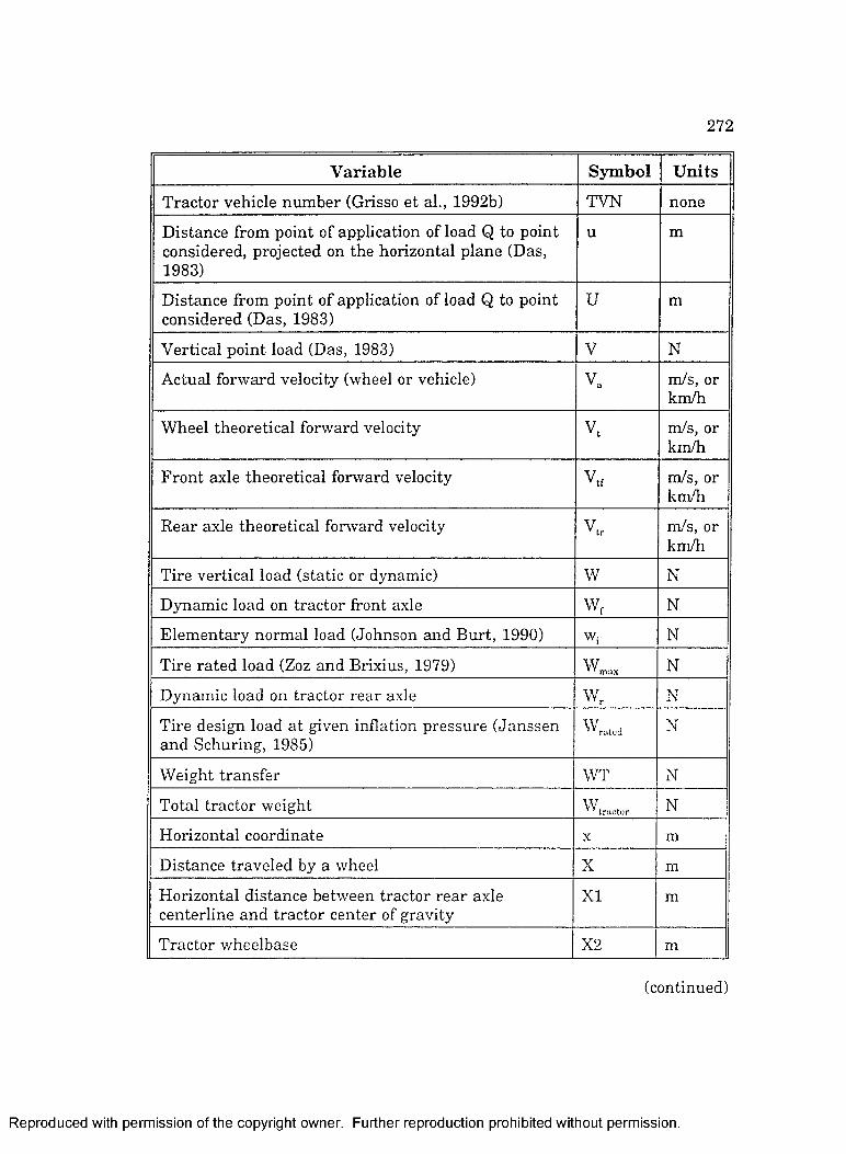
272
Variable Symbol Units
Tractor vehicle num ber (Grisso et al., 1992b) TVN none
Distance from point of application of load Q to point considered, projected on the horizontal plane (Das, 1983)
u m
Distance from point of application of load Q to point considered (Das, 1983)
U m
Vertical point load (Das, 1983) V N
Actual forward velocity (wheel or vehicle) V. m/s, or km/h
Wheel theoretical forward velocity V. m/s, or km/h
F ront axle theoretical forward velocity V.r m/s, or km/h
R ear axle theoretical forward velocity m/s, or km/h
Tire vertical load (static or dynamic) w N
Dynamic load on tractor front axle Wr N
Elem entary norm al load (Johnson and B urt, 1990) Wi N
Tire ra ted load (Zoz and Brixius, 1979) N
Dynamic load on tractor rear axle w . N
Tire design load a t given inflation pressure (Janssen and Schuring, 1985)
N
W eight transfer WT N
Total tractor weight W* t r a c to r N
Horizontal coordinate X m
Distance traveled by a wheel X m
Horizontal distance between tractor rea r axle centerline and tractor center of gravity
XI m
Tractor wheelbase X2 m
(continued)
R eproduced with perm ission of the copyright owner. Further reproduction prohibited without perm ission.

2 7 3
V a ria b le S ym bol U n its
Perpendicular distance from the line of action of ID to the point of action of the rear axle soil reaction
X3 m
H eight of the hitchpoint above the level of the point of application of the ear soil reaction (or draw bar height)
X4 m
Horizontal distance between tractor rea r axle centerline and hitchpoint
X5 m
Horizontal coordinate y m
Vertical coordinate, vertical distance from soil surface, depth of wheel sinkage or ru t depth
z m
O rdinate of first point on pressure-sinkage curve in Bekker (1960) sinkage prediction method
Zl m
O rdinate of second point on pressure-sinkage curve in Bekker (1960) sinkage prediction method
Z2 m
Angle of ID w ith the horizontal a rad, or deg
Spissitude (Freitag, 1966) P s.Pa
Soil specific w eight (Freitag, 1966) 1 N/m"
O ctahedral shear stra in (Johnson and B urt, 1990) To none
Stationary tire deflection 5 m
Deflection a t design load (Janssen and Schuring, 1985)
m
Stiffness vs. inflation pressure dependence coefficient (Lines and M urphy, 1991)
AK, kN/bar.m
Angle between the direction of a load and the projection on the horizontal plane of the line joining the point of application of the load to the point considered (Das, 1983)
e rad, or deg
Correction factor in tire-soil contact model (Upadhyaya and Wulfsohn, 1990)
n none
(continued)
R eproduced with perm ission of the copyright owner. Further reproduction prohibited without perm ission.

2 7 4
Variable Symbol Units
Tire-soil friction coeffrdent P none
Gross traction ratio none
N et traction ratio Pm none
Transm ission effidency between PTO and front axle Pptofa none
Transm ission effidency between PTO and rea r axle Pptora none
Transm ission effidency Pt none
Tractive power ratio (Persson, 1991) Ptp none
Poisson ratio V none
Correction factor in tire-soil contact model by U padhyaya and W ulfsohn (1990)
none
jr-terms used in dimensional analysis (Freitag, 1966) 7T], TÏ2,
JC7, Kg,
9> ^ 10>
none
D istance of point from center of circular area (Soehne, 1958)
Pc m
Angle between the vertical direction and the line join ing the point of application of load Q to the point considered (Das, 1983)
(p rad, or deg
Normal stress a t the soil-tire contact surface (Wulfsohn and Upadhyaya, 1991)
G, Pa
Radial soil stress in cylindrical coordinates (Das, 1983)
Gu Pa
Soil norm al stress in the x direction (Das, 1983) Gx P a
Soil norm al stress in the y direction (Das, 1983) 0y Pa
Soil norm al stress in the z direction (Das, 1983) Pa
Tangential soil stress in cylindrical coordinates (Das, 1983)
0 , Pa
(continued)
R eproduced with perm ission of the copyright owner. Further reproduction prohibited without perm ission.

275
V a ria b le S ym bo l U n its
S hear stress a t soil-tire contact surface (Wulfsohn and U padhyaya, 1991)
X P a
O ctahedral shear stress (Johnson and Burt, 1990) -Co Pa
Soil shear stress in cylindrical coordinates (Das, 1983)
Pa
Soil shear stress in the xy plane (Das, 1983) Pa
Soil shear stress in the xz plane (Das, 1983) Pa
Soil shear stress in the yz plane (Das, 1983) V . P a
Soil friction coefficient rad, or deg
Angle between the surface normal and the vertical at any point on the soil-tire contact surface (Wulfsohn and Upadhyaya, 1991)
d ) rad, or deg
V ertical angle from tire axle to a point on the contact surface (Wulfsohn and Upadhyaya, 1991)
Y rad, or deg
Wheel angular velocity D rad/s, or rpm
Tractor front axle angular velocity D, rad/s, or rpm
Tractor rear axle angular velocity
. ............
D, rad/s,or rpm
R eproduced with perm ission of the copyright owner. Further reproduction prohibited without perm ission.

APPENDIX B MANUFACTURER DATA FOR SENSORS
USED ON LSU TIRE-LOADING MACHINE
Load CellsM an u factu rer D ata
M anufacturer: BLH Electronics, 42 Fourth Avenue, W altham , M assachusetts 02157.Model: U3L1 Capacity: 22.240 kNRecommended excitation voltage: 15 V ac-dc M aximum excitation voltage: 20 V ac-dc Inpu t resistance: 350+3.5 O utput resistance: 350±5.0 Ü Insulation resistance: 5 GO.R ated output (RO): 3 mVA^±0.25% in compression, 3 mVW±0.5% in tensionZero balance: 1.0% RONonlinearity: 0.10% ROHysteresis: 0 .10% RORepeatability: 0 .02% ROCreep: 0.05% ROTem perature effect on zero balance: 0.0027% RO/°CTem perature effect on output reading: 0.0027% RO/°CCompensated tem perature range: -9.4° to h-46.1°CSafe tem perature range: -53.9°C to 93.3°CSafe overload capacity: 150% CapacityU ltim ate overload: 300% CapacitySideload: 100% CapacityBending moment: 1.27% Capacity in NmTorque load: 0.76% Capacity in NmConnection (cable or connectors): Bendix
C a l i b r a t i o n C u r v e s
The 3 load cells were calibrated with an INSTRON model 1332 electro-
hydraulic press belonging to the Mechanical Engineering D epartm ent at LSU.
The linear regression equations for the calibration curves were:
276
R eproduced with perm ission of the copyright owner. Further reproduction prohibited without perm ission.

2 7 7
For load cell #1,
Reading (kN) = 0.014775 + 1.005837 * Actual load (kN) (R ^=0.909)
For load cell #2,
R eading (kN) = -0.01154 + 1.000915 * Actual load (kN) (iî >0.999)
For load cell #3,
Reading (kN) = -0.00016 + 1.00147 * Actual load (kN) (J2“>0.999)
25
20
15
10
5
05 10 15
A C T U A L L O A D ( k N )
F igu re B l. C alibration curve for load cell #1.
R eproduced with perm ission of the copyright owner. Further reproduction prohibited without perm ission.

278
zM
z5<moia
i
25
20
J5
10
5
00 5 10 13 20 23
ACTUAL LOAD (kN))
F igu re B2. C alibration curve for load ce ll #2.
25
20
15
10
5
05 10 15 200
ACTUAL LOAD (kN)
F ign re B3. C alibration curve for load cell #3.
R eproduced with perm ission of the copyright owner. Further reproduction prohibited without perm ission.

2 7 9
Linear Displacement TransducerM an u factu rer D ata
M anufacturer: Penny and Giles Position Sensors Ltd, Somerford Road C hristchurch, D orset BH23 3RS U nited Kingdom.Type and model: H ybrid track rectilinear potentiom eter, long stroke modelHLP 350/SA 600Mounting: Self aligning bearingsShaft type: free floatingElectrical stroke: 600 mmResistance ± 10%: 24 kOIndependent linearity: ± 0.15%Power dissipation a t 20°C: 12 W Applied voltage (maximum): 130 VLim iting voltage: 130 V or (power dissipation x resistance)^ (whichever is less)Resolution: V irtually infiniteO perational tem perature range: -50°C to +85°CO utput smoothness: to MIL-R-39023 grade C 0.1%Insulation resistance a t 500 V d.c.: g reater than 100 MQLife a t 250 mm/s: typically g reater than 50 x 10® cycles a t 25 mm stroke lengthM axim um shaft velocity: 1000 mnVsElectrical output: single electrical output, minimum of 0.5% to 99.5% applied voltsShaft seal: felt dust sealO perating force maximum: 10 N in horizontal plane O perating mode: voltage divider onlyW iper circuit impedance: minimum of 100 x track resistance or 0.5 MO (whichever is greater)M echanical/electrical stroke (M/E): 600 mm Electrical stroke tolerance: ± 0.75 mm Body length, B: 759 mm D istance between centres, D: 860 mm Mass: 1.670 kg
C alib ration C urve
The displacem ent transducer was calibrated with an engineering ruler.
The linear regression equation obtained was.
R eproduced with perm ission of the copyright owner. Further reproduction prohibited without perm ission.

280
R e a d i n g { m m ) = -4.242 + 1.000 * A c tu a l d i s p i . ( m m ) {R ^ = 0.999)
700
E 600
500
400
300
200200 300 400 500 600 700
ACTUAL DISPLACEMENT (mm)
F igu re B4. C alibration curve for the d isp lacem en t transducer.
In fla tio n P re s s u re GageThe inflation pressure gage used for the LSU experim ents was a generic
tire pressure gage bought from an automotive accessory shop. The gage was
calibrated w ith a Heise (Newtown, Connecticut) 0-100 psi high precision air
pressure gage belonging to the Mechanical Engineering D epartm ent a t LSU.
The linear regression equation obtained was,
R e a d i n g ( k P d ) = 7.636 + 1.005 * A c tu a l p r e s s . ( k P a ) (R ^ = 0.999)
R eproduced with perm ission of the copyright owner. Further reproduction prohibited without perm ission.

281
I 300
iû 250
swO 200
Swa;D 15000on
gCÜ 100
<Ju îogSg 0
100 150 200 250
REFERENCE AIR PRESSURE GAGE READING (kPa)
F ig u r e B 5 . C a lib r a tio n c u r v e fo r th e in f la t io n p r e s s u r e g a g e .
R eproduced with perm ission of the copyright owner. Further reproduction prohibited without perm ission.

APPENDIX C TIRE AND TUBE DATA
T able C l. T ire-T ube M atching TableNum ber
andm ass
Tire m odel and
arrival batch
Tube, arrival batch, num ber
and mass
Rimm odel
No. 173.91 kg
&No. 2
73.91 kg
14.9-30 BATCH 2 HI TRACTION LUG All purpose R-1 10 ply rating 221 kPa (max operating pressure) tubeless
650010/15014 BATCH 2 Rear Tractor Tube, No. 1 Not usable in 7.71 kg radial tires No. 2 16.9/14-30, 7.71 kg 18.4/15-30, 14.9/13-30
W13-30
No. 394.31 kg
&No. 4
94.31 kg
14.9R30 BATCH 1HI TRACTION LUGRADIALAll purpose R-1*** rated load: 22.3 kNrated inf].: 207 kPatubeless134A8
650010/15014 BATCH 2 Rear Tractor Tube, No. 1 Not usable in 7.71kg radial tires No. 2 16.9/14-30, 7.71 kg 18.4/15-30, 14.9/13-30
W13-30
No. 5 62.12 kg
&No. 6
63.25 kg
16.9-30 BATCH 2 HI TRACTION LUG All purpose R-1 6 ply rating 124 kPa (max operating pressure)
650010/15014 BATCH 2 Rear Tractor Tube, No. 5 Not usable in radial 7.48 kg tires No. 6 16.9/14-30, 7.71 kg 18.4/15-30, 14.9/13-30
WH15L-30
No. 7 113.13 kg
&No. 8
112.22 kg
16.9R30 BATCH 2HI TRACTION LUGRADIALAll purpose R-1** rated load: 24.2 kNrated infl.: 165 kPatubeless137A8
650010/15014 BATCH 2 Rear Tractor Tube, No. 7 Not usable in 7.93 kg radial tires No. 8 16.9/14-30, 7.82 kg 18.4/15-30, 14.9/13-30
WH15L-30
No. 9 82.75 kg
&No. 10
82.97 kg
18.4-30 BATCH 1 HI TRACTION LUG All purpose R-1 8 ply rating 138 kPa (max operating pressure)
650010/15014 BATCH 1 Rear Tractor Tube No. 9 Not us&M ihg radial tiresNo. 10 16.9/14-30, 18.4/15-30 7.93 kg
WH15L-30
(continued)
282
R eproduced with perm ission of the copyright owner. Further reproduction prohibited without perm ission.

283
Num berand
m ass
Tire m odel and
arrival batch
Tube, arrival batch, num ber
and m ass
R imm odel
No. 11 59.85 kg
&No. 12
60.98 kg
15.5-38 BATCH 1 HI TRACTION LUG All purpose R-1 6 ply rating 138 kPa (max operating pressure)
R50008/15008 BATCH 1 Fieldmaster Radial No. 11 Tractor Tube, 7.48 kg Approved for use in No. 12 radial or bias tires 7.93 kg 13.6/12-38, 14.9/13-38, 15.5-38,13.6R38, 14.9R38, 15.5R38
WH14L-38
No. 13 63.02 kg
&No. 14
61.66 kg
15.5-38 BATCH 2 HI TRACTION LUG All purpose R-1 6 ply rating 138 kPa (max operating pressure)
R50008/15008 BATCH 2 Fieldmaster Radial No. 13 Tractor Tube 7.93 kg Approved for use in No. 14 radial or bias tires 7.71kg 13.6/12-38, 14.9/13-38,15.5-38, 13.6R38, 14.9R38, 15.5R38
WH14L-3S
No. 15 78.89 kg
&No. 16
79,35 kg
16.9-38 BATCH 2 HI TRACTION LUG All purpose R-1 6 ply rating 124 kPa (max operating pressure)
R50012/15012 BATCH 2 Premium Fieldmaster No. 15 Radial Tractor Tube. 9.98 kg Approved for use in No. 16 radial or bias tires 10.20 kg 16.9R38, 18.4R38 16.9/14-38, 18.4/15-38
WH14L-38
No. 17 94.99 kg
&No. 18
98.39 kg
18.4-38 BATCH 2 HI TRACTION LUG All purpose R-1 6 ply rating 110 kPa (max operating pressure)
52405 BATCH 2 Premium Fieldmaster No. 17 Radial Tractor Tube, 9.98 kg Approved for use in No. 18 radial or bias tires 9.98 kg 16.9R38, 18.4R38
W16L-3S
No. 19 145.09 kg
&No. 20
142.37 kg
18.4R38 BATCH 1 HI TRACTION LUG RADIAL All purpose R-1 * rated load: 27.0 kN rated infl.: 124 kPa
R50012/15012 BATCH 1 Fieldmaster Radial No. 19 Tractor Tube 9.98 kg Approved for use in No. 20 radial or bias tires 9.98 kg 16.9R38, 18.4R38,16.9/14-38, 18.4/15-38
W16L-38
R eproduced with perm ission of the copyright owner. Further reproduction prohibited without perm ission.
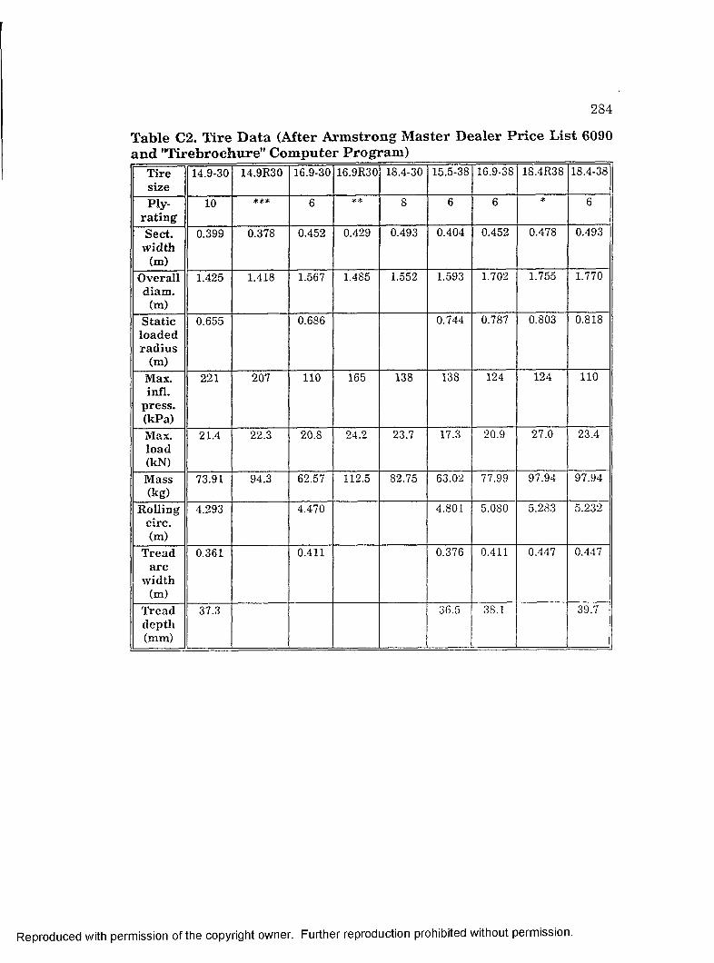
284
T able C2. T ire D ata (After A rm strong M aster D ealer P r ice L ist 6090 and "Tirebrochure" C om puter Program )
T ires ize
14.9-30 14.9R30 16.9-30 16.9R30 18.4-30 15.5-38 16.9-38 18.4R38 18.4-38
P ly-r a tin g
10 *** 6 8 6 6 * 6
S ect.w id th
(m)
0.399 0.378 0.452 0.429 0.493 0.404 0.452 0.478 0.493
O veralld iam .
(m)
1.425 1.418 1.567 1.485 1.552 1.593 1.702 1.755 1.770
S ta ticlo a d edra d iu s
(m)
0.655 0.686 0.744 0.787 0.803 0.818
M ax.in fl.
p ress .(kPa)
221 207 110 165 138 138 124 124 110
Max.load(kN)
21.4 22 3 2&8 24^ 23.7 17.3 2&9 27.0 2&4
M ass(kg)
73.91 94.3 62.57 112.5 82.75 63.02 77.99 97.94 97.94
R o llin gcirc.(m)
4.293 4.470 4.801 5.080 5.283 5.232
T readarc
w idth(m)
0.361 0.411 0.376 0.411 0.447 0.447
T readdepth(mm)
3TJ 3&5 38T 3&7
R eproduced with perm ission of the copyright owner. Further reproduction prohibited without perm ission.

285
T able C3. R ated T ire L oads (After T ire and Rim A ssocia tion , 1989, and A rm stron g T ire Load C alcu lation E quations)
T ires ize
T ire lo a d lim its (kN) at v a r io u s co ld in fla tio n p ressu res (kPa)
83 97 110 124 138 152 165 179 193 207
14.9R30 12.9 14.1 15.3 16.3 17.4 18.5 19.4 20.4 21.2 22 3
14.9-30 12.1 13.2 14.3 15.3 16.3 17.2 18.1 19.0 1&8 2Œ8
16.9R30 15.7 17.2 18.5 19.9 21.1 22.4 24^
16.9-30 14.7 16.1 17.3 18.6
18.4-30 17.6 19.2 20.8 2&3 23.7
15.5-38 12.9 14.1 15.2 16.3 17.3
16.9-38 16.5 18.1 19.5 20.9
18.4R38 21.1 23.1 24.0 27.0
18.4-38 19.8 21.6 2&4
N ote: Loads can be increased by 20% for bias-ply tires used below 16 knidi, and by 34% for radiais below 16 km/h.
R eproduced with perm ission of the copyright owner. Further reproduction prohibited without perm ission.

APPENDIX D SAMPLE STATIC LOAD-DEFLECTION
DATA AND TESTS PERFORMED
T able D l. Sp read sh eet F ile C onta in ing L oad-D eflection D ata05-04-1993 05:42:53 stat.acq 5
CHANNELS0.009167MINS
CHANNEL 1 2 3 4 5 BINARYTime EXCITA
TIONLC l LC2 LC3 LDT INPUTS
Seconds Volts lbs lbs lbs in0 -4.6357 81.56666 109.9227 59.61414 -4.17134 00.5053 -4.6805 73.09282 101.6958 50.86758 -4.21469 01.0552 -4.72108 65.3177 94.17262 42.86681 -4.2544 01.6053 -4.75771 58.21106 87.30263 35.61657 -4.29014 02.1552 -4.7909 51.70605 81.06017 29.04179 -4.32287 02.7053 -4.82098 45.87137 75.41223 23.05511 -4.35135 03.2553 -4.84817 40.5706 70.26961 17.65719 -4.37698 0
286
R eproduced with perm ission of the copyright owner. Further reproduction prohibited without perm ission.

2 8 7
Table D2. R anges o f Inflation Pressure and Num ber of Tests Perform ed U nder Static Conditions for Each Tire
Tire Low est inflation pressure tested
(kPa)
H ighest inflation pressure tested
(kPa)
Total num ber o f static
tests
14.9-30 #1 41 221 28
14.9-30 #2 41 221 28
14.9R30 #3 41 207 26
16.9-30 #5 41 124 14
16.9R30 #7 41 165 20
18.4-30 #9 41 138 16
15.5-38 #11 41 138 156
15.5-38 #13 41 138 16
16.9-38 #15 41 124 14
18.4-38 #17 41 110 12
18.4R38 #20 41 124 14
R eproduced with perm ission of the copyright owner. Further reproduction prohibited without perm ission.

APPENDIX E PROGRAM ECC2.FOR AND
SAMPLE RESULTS
Program ECC2.FORcC Francois BRASSART - LSU, Bio. & Ag. Eng, Dept. - 03/27/92 CC Program EC C 2.F0R - Metric units version of ECC.FOR C This program computes the motion of a piston driven by a C rod of length R and an eccentric of length E. The C velocities and accelerations are also computed. The C vertical motion of the piston is compared to a simple C vertical sinusoidal motion.CC Y: actual vertical positionC DY: actual vertical velocityC DDY: actual vertical acceleration C YR: reference sinusoidal position C DYR: reference sinusoidal velocity C DDYR: reference sinusoidal acceleration C TH: angle C OM: angular velocityC AT,L,L0,R1,R2,R3,R4,R5,R6,Y1,Y2,Y3,Y4,Y5,Y6,YR1,YR2,YR3,YR4, C YR5,YR6,DY3,DY4,DY5,DY6,DYR3,DYR4,DYR5,DYR6,D25,D26,C DR25,DR26,DIF,DDF,DDD: auxiliary calculation variables C
REALE,R,L0,0M,PI,DTR,RTD,T(181),TH(181),L(1S1),Y(181),C YR(181),DIF(181),AT,DY(181),DDY(181),DYR(181),C DDYR(181),R1,R2,R3,R4,R5,R6,Y1,Y2,Y3,Y4,Y5,Y6,YR1,YR2,C YR3,YR4,YR5,YR6,DY3,DY4,DY5,DY6,DYR3,DYR4,DYR5,DYR6, C D25,D26,DR25,DR26,DDF(18i),DDD(181)CHARACTER*! ANS PI=AC0S(-1.) RTD=180/PI DTR=PI/180
CC DEFAULT DATA, E AND R IN meters, OM IN rpm C
E=0.0127R=0.78105
288
R eproduced with perm ission of the copyright owner. Further reproduction prohibited without perm ission.

289
OM=200.LO=R*COS(ASIN(E/R))
CC INITIALIZE AUXILIARY VARIABLES C
Rl=-100000R2=100000R3=-100000R4=100000R5=-100000R6=100000
CC POSSIBILITY TO INPUT NEW VALUES C
PRINT*,TOU WANT TO: ENTER NEW DATA - > PRESS 1’PRINT*,' USE DEFAULT VALUES —> PRESS 2’READ(5,12) ANS
12 FORMAT(Al)IF(ANS.EQ.’1’)THEN WRITE(5,13) E
13 F0RMAT(2X,’ENTER ECCENTRIC LENGTH E IN m <’F7.5,’>:’) READ(5,*) EWRITE(5,14) R
14 F0RMAT(2X,’ENTER ROD LENGTH R IN m <’F7.5,’>:’) READ(5,*) RWRITE(5,15) OM
15 F0RMAT(2X,’ENTER ANGULAR VELOCITY IN rpm <’,F7.2,'>:’) READ(5,*) OM
ELSECONTINUE
ENDIFCC OPEN RESULT FILE C
OPEN(2,FILE=’ECC.RES’,STATUS=’old’)CC HEADER C
WRITE(2,11) E,R,OM C WRITE(2,10)
WRITE(6,10)11 F0RMAT(5X,'PROGRAM ECC2.F0R '/,
C 5X,'INPUTS FOR COMPUTATION OF PISTON-ROD MOTION'/, C 5X,'eccentric length : E = ',F7.5,'m'/,5X,
R eproduced with perm ission o f the copyright owner. Further reproduction prohibited without perm ission.

2 9 0
C ’rod length : R = ’,F7.5,'m '/,5X,C ’angular velocity : OM = ’,F7.2,’rpm ’/y ,C 5X,’OUTPUTS’/)
10 F0RMAT(7X,’TIME’,3X,’ANGLE’, IX,C ’L0C A T I0N ’,1X,’REF. SIN’,4X,’DIFF.’,6X,’DY’,5X,’DYR’,0 6X,’DDY’,5X,’DDYR’/C 8X,’s’,6X,’deg.’,7X,’m’,8X,’m’,8X,’m ’,6X,’m/s’,C 5X ,W s’,4X,’m/s^2’,4X,’m/s/'2’)
CC CONVERT OM FROM rpm TO rad/s C
OM=OM*2.*PI/60.CC COMPUTE POSITION, VELOCITY AND ACCELERATION EVERY 2 DEC. C
DO 20 1=1,181 T(I)=(I-1)*2.*PI/(180/OM)TH(I)=OM*T(I)L(I)=E*SIN(TH(I))+R*COS(ASIN(E*COS(TH(I))/R))Y(I)=L(I)-RYR(I)=E*SIN(TH(D)DIF(I)=Y(I)-YR(I)IF(DIF(I).LT.O.)THENDIF(I)=-DIF(I)
ENDIFDYR(I)=OM*E*COS(TH(D)DDYR(I)=-OM*OM*E*SIN(TH(I))DY(I)=0M*E*C0S(TH(I))*(1+(E*SIN(TH(I))/
C (R*SQRT(1-(E*C0S(TH(I))/R)**2)))) AT=SQRT(1-((E*C0S(TH(I))/R)**2)) DDY(I)=E*0M*0M*(-SIN(TH(I))*(1+E*SIN(TH(I))/(R*AT))
C +(E*C0S(TH(I))/R)*(C0S(TH(I))*AT*AT-((SIN(TH(I))**2)*E)C /(2*R))/(AT**3))
DDF(I)=DY(I)-DYR(I)IF(DDF(I).LT.O.)THENDDF(I)=-DDF(I)
ENDIFDDD(I)=DDY(I)-DDYR(I)IF(DDD(I).LT.O.)THENDDD(I)=-DDD(I)
ENDIFTH(I)=TH(I)*RTDWRITE(6,30) T(I),TH(I),Y(I),YR(I),DIF(I),DY(I),DYR(I),
C DDY(I),DDYR(I)
R eproduced with perm ission of the copyright owner. Further reproduction prohibited without perm ission.
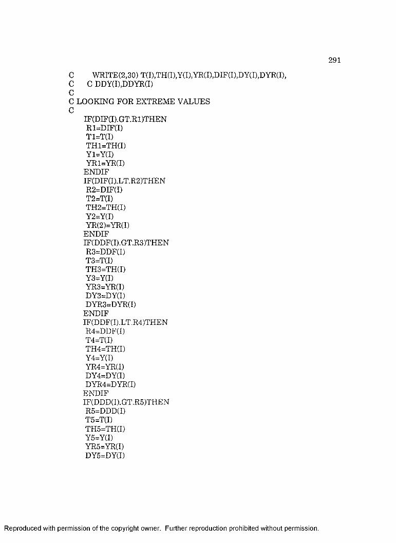
2 9 1
C WRITE(2,30) T(I),TH(I),Y(I),YR(I),DIF(I),DY(I),DYR(I), C C DDY(I),DDYR(I)CC LOOKING FOR EXTREME VALUES C
IF(DIF(I).GT.R1)THENR1=DIF(I)T1=T(I)T H 1=TH(I)Y1=Y(I)YR1=YR(I)
ENDIFIF(DIF(I).LT.R2)THENR2=DIF(I)T2=T(I)TH2=TH(I)Y2=Y(I)YR(2)=YR(I)
ENDIFIF(DDF(I).GT.R3)THENR3=DDF(I)T3=T(I)TH3=TH(I)Y3=Y(I)YR3=YR(I)DY3=DY(I)DYR3=DYR(I)
ENDIFIF(DDF(I).LT.R4)THENR4=DDF(I)T4=T(I)TH4=TH(I)Y4=Y(I)YR4=YR(I)DY4=DY(I)DYR4=DYR(I)
ENDIFIF(DDD(I).GT.R5)THENR5=DDD(I)T5=T(I)TH5=TH(I)Y5=Y(I)YR5=YR(I)DY5=DY(I)
R eproduced with perm ission of the copyright owner. Further reproduction prohibited without perm ission.

292
DYR5=DYR(I)D25=DDY(I)DR25=DDYR(I)
ENDIFIF(DDD(I).LT.R6)THENR6=DDD(I)T6=T(I)TH6=TH(I)Y6=Y(I)YR6=YR(I)DY6=DY(I)DYR6=DYR(I)D26=DDY(I)DR26=DDYR(I)
ENDIF20 CONTINUE30 FORMAT(5X,F6.3,2X,F6.2,2X,F7.5,2X,F7.5,2X,F7.5,2X,F6.4,2X,
C F6.4,2X,F7.4,2X,F7.4)WRITE(6,40)T1,TH1,Y1,YR1,R1,T2,TH2,Y2,YR2,R2WRITE(6,41)T3,TH3,Y3,YR3,DY3,DYR3,R3,
C T4,TH4,Y4,YR4,DY4,DYR4,R4WRITE(6,42) T5,TH5,Y5,YR5,DY5,DYR5,D25.DR25,R5,
C T6,TH6,Y6,YR6,DY6,DYR6,D26,DR26,R6 WRITE(2,40) T1,TH1,Y1,YR1,R1,T2,TH2,Y2,YR2,R2 WRITE(2,41) T3,TH3,Y3,YR3,DY3,DYR3,R3,
C T4,TH4,Y4,YR4,DY4,DYR4,R4 \VRITE(2,42) T5,TH5,Y5,YR5,DY5,DYR5,D25,DR25,R5,
CT6,TH6,Y6,YR6,DY6,DYR6,D26,DR26,R640 F0RMAT(5X,’Maximum difference in location y:’,/,6X,
C Time = ’,F7.2,'s’,9X,'Angle = ’,F7.2,'deg.’/,C 6X,'Location = ',F7.5,'m',5X,C 'Ref. location = ',F7.5,'m',3X,'Diff. = ’,F9.7,C'm'/,C 5X,'Minimum difference in location y;',/,6X,C Time = ',F7.2,'s',9X/Angle = ',F7.2,'deg'/,C 6X,location = ',F7.5,'m',5X,C 'Ref. location = ',F7.5/m',3X,'Diff. = ',F9.7,C m ')
41 F0RMAT(5X,'Maximum difference in velocity dy:'/,6X,C Tim e = ',F7.2,'s',9X,'Angle = ',F7.2,'deg'/,C 6X,'Location = ',F7.5,'m’,5X,C 'Ref. location = ',F7.5,'m '/,6X,'Velocity = ',F7.4,C 'm/s',3X,'Ref. velocity = ',F7.4,'m/s',C 2X,'Diff. = ',F9.7,'m/s'/,
R eproduced with perm ission of the copyright owner. Further reproduction prohibited without perm ission.

293
C 5X,’M inimum difference in velocity dy;V.6X,C T im e = ’,F7.2,’s’,9X,’Angle = ’,F7.2,’deg’,/,C 6X,’Location = ’,F7.4,’m’,5X,C ’Réf. location = ’,F7.4,’m’/ , 6X,’Velocity = ’,F7.4,C ’m/s’,3X,’Réf. velocity = ’,F7.4,’m/s’,C 2X,’Diff. = ’,F9.7,’m/s’)
42 F0RMAT(5X,’Maximum difference in acceleration ddy:’/, C 6X,Tim e = ’,F7.2,’s’,9X,’Angle = ’,F7.2,’deg’/C 6X,’Location = ’,F7.4,’m’,5X,C ’Réf. location = ’,F7.4,’m’/,6X ,’Velocity = ’,F7.4,C ’m/s’,3X,’Réf. velocity = ’,F7.4,’m/s’/,C 6X,’Accel. = ’,F7.4,’m/s^2’,3X,C ’Réf. accel. = ’,F7.4,’m/s^2’,C 2X,’Diff. = ’,F9.6,’m/s^2’y,C 5X,’M inimum difference in acceleration ddy:’/ , 6X,C Tim e = ’,F7.2,’s’,9X,’Angle = ’,F7.2,’deg’/,C 6X,’Location = ’,F7.4,’m’,5X,C ’Réf. location = ’,F7.4,’m’/,6X ,’Velocity = ’,F7.4,C ’m/s’,3X,’Ref. velocity = ’,F7.4,’m/s’/,C 6X,’Accel. = ’,F7.4,’m/s^2’,3X,C ’Réf. accel. = ’,F7.4,’m/s^2’,C 2X,’Diff. = ’,F9.6,’m/s^2’)CL0SE(2)STOPEND
S am ple R esu ltsPROGRAM ECC2.F0RINPUTS FOR COMPUTATION OF PISTON-ROD MOTION eccentric length : E = .01270m rod length : R = .74295mangular velocity : OM = 200.00rpm
OUTPUTS
Maximum difference in location y:Time = .00s Angle = .OOdeg.Location = -.00011m R ef location = .00000m Diff. = .0001086m
Minimum difference in location y:Time = .23s Angle = 270.OOdegLocation = -.01270m R ef location = .00000m Diff. = .0000000m
Maximum difference in velocity dy;
R eproduced with perm ission of the copyright owner. Further reproduction prohibited without perm ission.

2 9 4
Time = .04s Angle = 44.OOdegLocation = ,00877m Ref. location = .00882m Velocity = .1936m/s Ref. velocity = .1913m/s Diff. = .0022722m/s
^Minimum difference in velocity dy:Time = .00s Angle = .OOdegLocation = -.0001m Ref. location = .0000mVelocity = .2660m/s Ref. velocity = .2660m/s Diff. = .OOOOOOOm/s
M aximum difference in acceleration ddy:Time = .15s Angle = 180.OOdegLocation = -,0001m Ref. location = ,0000mVelocity = -,2660m/s Ref. velocity = -,2660m/sAccel. = .0952m/s'^2 R ef accel. = .0000m/s^2 Diff. = .095242m/s^2
M inimum difference in acceleration ddy:Time = ,11s Angle = 134.OOdegLocation = ,0091m Ref. location = ,0091mVelocity = -,1870m/s Ref. velocity = -,1848m/sAccel. = -4.0104m/s^2 Ref. accel. = -4.0073m/s'^2 Diff. = .003031m/s'^2
R eproduced with perm ission of the copyright owner. Further reproduction prohibited without perm ission.

APPENDIX F SAMPLE DYNAMIC LOAD-DEFLECTION
DATA
T able F I. S p read sh eet F ile C onta in ing D ynam ic L oad-D eflection D ata09-28-1993 15:13:07 dyn.acq 6
CHANNELS
0.00091 7 MINS
CHANNEL 1 2 3 4 5 6 DINARY
Time EXCITATION
LC l LC2 LC3 LDT TACHO INPUTS
Seconds Volts lbs lbs lbs in. Volts0 -4.35621 -268.324 - 2 5 1 .9 9 4 -291.938 -6.84204 -0.75042 00.016 -4.35011 - 2 2 3 .7 9 9 -208.409 - 2 4 6 .3 5 5 -6.72725 -0.70827 00.071 -4.35621 -186.911 - 1 8 0 .5 6 7 -202.065 -6.55425 -0.67229 00 .1 2 6 -4.34462 - 1 6 2 .2 4 -159.773 -172.578 -6.45111 -0.59413 00.181 -4.35194 -153.194 -148.025 -157.893 -6.36627 - 0 .7 4 0 6 2 00.2361 -4.34523 -153.194 -146.615 -157.893 -6.37459 -0.80898 00.2911 -4.35041 -173.87 -162.592 -184.209 - 6 .4 4 4 4 6 -0.76312 0
2 9 5
R eproduced with perm ission of the copyright owner. Further reproduction prohibited without perm ission.

296
T able F2. R an ges o f Inflation P ressu re and N um ber o f T ests P erform ed U nd er D ynam ic C onditions for E ach Tire
T ire L ow est in fla tion pressu re tested
(kPa)
H igh est in fla tion pressu re tested
(kPa)
T ota l num ber o f dynam ic
te sts
14.9-30 #1 41 221 168
14.9-30 #2 41 2 2 1 168
14.9R30 #3 41 207 156
16.9-30 #5 41 124 84
16.9R30 #7 41 165 120
18.4-30 #9 41 138 96
15.5-38 #11 41 138 96
15.5-38 #13 41 138 96
16.9-38 #15 41 124 84
18.4-38 #17 41 110 72
18.4R38 #20 41 124 84
R eproduced with perm ission of the copyright owner. Further reproduction prohibited without perm ission.

APPENDIX G
SAMPLE CONE INDEX, ROLLING RADIUS AND TRACTION DATA
297
R eproduced with perm ission of the copyright owner. Further reproduction prohibited without perm ission.

298
-W
QC/I
.2CÏ
Kt£a
Bêfeuc
'3*S-w0o
Ü
«
-wQJ0)
X7)
'3
aœ
Ü3)
IH
aXT
d
i n00CO*H
00o(N
04od
0404d
C5oCDd
o -CDod
Z
or -oo
(NCOr-4rHd
COTT00d
04CD04od
CDCDod
oo -
d
TTood
UO
COera
<NTTo
COCO orHo-V
CD00CD
sc -
(N (N 04 04 04 04
%CO00 CO
'VCOCO c- XT
rH'TrH 04
CO CO C5 CO o- in
S CD(N
œCO
COin
CDCD 00
H o o o o o o
Ü 00 (N o CO CD TTCOCO inCO
CDCO CO2
o CO0-
22Q
COCOoino o
CDo
CD0404in
*-4 r-i
o
(No(N
TTXTo(M
<N(TioCM
TP'TT
04CDo04
oCDo04
-rf
o04
o o o o o o o
u
>
COr-2
in in"V
04CD
04(DTT
04r4in
0004in
o o o o o o oCO 00 04 in D
CiOj 00
CO00CO
r-CO
002
COCO 0-
2 CO
êp
CO CD tt rr CD CD 04lOoOf
ino(NCDotN
CDo04
CDo04
CDo04o-ooq
Q
TT Tf 04 CD DCOTf CD
sCD CO CD in
TTin
Cio00TfCO<No
CDoinod
ooo
COCO04od
0-
COd
04TTo04d
oo<d
o p%COo
CO<MCOCDCO
COCDCOTTCD
0000o-
cc00O'
(N C4 04 04 04 04
Q<Nn
tT2
00'rr2
inTT COCDo
inCD
ino-CDin04
+ o o o o o od o
CO>
lOrH
TT(M<N
00o04
o04o
TfoinCO
TT04CO04
CDCOtt04
o o o o o d dII
Ci>
lOCT5o
CO-Vd
0004od
in00CDod
CO04oo
T-COCOd
COCO0404d
OQTTCvJCOo p COo
CDo00(N
ccCO03rr
inCOo
in
2
04CO04
inTT04
Ci o o o o o o o
R eproduced with perm ission of the copyright owner. Further reproduction prohibited without perm ission.

299
Table G2. Location and Filenames of Cone Index Measurements Before Traffic for the First Soil Bin Preparation, Norfolk Sandy Loam, V- Wheel Packed, Surface Leveled With Scraper Blade
N Î
106351.dat 106352.dat 106353.dat 106354.dat 106355.dat 106356.dat106341.dat 106342.dat 106343.dat 106344.dat 106345.dat 106346.dat106331.dat 106332.dat 106333.dat 106334.dat 106335.dat 106336.dat106321.dat 106322.dat 106323.dat 106324.dat 106325.dat 106326.dat106311.dat 106312.dat 106313.dat 106314.dat 106315.dat 106316.dat
Each cone index data file contained:
• On the th ird row:
- The filename, with its directory extension according to NSDL data storage
schemes;
• On the fifth row, the names of the variables recorded during a test:
- Time (hh:mm:ss:ds): time (in hundredths of a second) of recording;
- Force (N): force applied to the cone penetrom eter tip;
- Depth (mm): location of the cone penetrom eter tip with respect to the frame
of the cone penetrom eter car.
® On the following rows, were the data;
• The first, second and fourth rows were empty.
R eproduced with perm ission of the copyright owner. Further reproduction prohibited without perm ission.

3 0 0
Table G3. Location and Filenames of the Cone Index Measurements Before Traffic for the Second Soil Bin Preparation, Norfolk Sandy Loam, V-Wheel Packed, Surface Leveled With Scraper Blade
nT107740.dat 107741.dat 107742.dat 107743.dat 107744.dat 107745.dat107730.dat 107731.dat 107732.dat 107733.dat 107734.dat 107735.dat107720.dat 107721.dat 107722.dat 107723.dat 107724.dat 107725.dat107710.dat 107711.dat 107712.dat 107713.dat 107714.dat 107715.dat107700.dat 107701.dat 107702.dat 107703.dat 107704.dat 107705.dat
R eproduced with perm ission of the copyright owner. Further reproduction prohibited without perm ission.

clceQaoueskHfccG
es-wcoüSi
9)S)en
'S3esükaco<
üCD
«H
CdH
COsC-o
LOIN0500d
(NCOd
inCOd
t-inCOind
in05rHt>d
8rHrH
Z
o00COCJ5d
TfCOc^d
0500o05d
CO inCO05d
COqi-H
rHrHIN
kdQ
INCOrH
GOINV
sin
0505IN
COcq
"VCOrH
05inœrH
5CO
rHTTd
lOd
(N■*r2
Nd d
IN
2
rHINTTrH
sp
o dCONd
00COd
md
INCOd
C~Cd
O 'Tf00*COrH
orH
cqr- rH
COdrH
t *2
CO05rH
COQ lOCO
CO'VdCO
indCO
COindCO
TTmdCO
COindCO
05indCO
gO
rHOlO(Nd
COr -tTINd
r-NTTINd
crrINd
rHTfINd
in[~-inINd
INd
u>
TTolOd
§lOd
ind
0000TTrHd
COTTind
CO05
d
oind
Ka.2
iqCO
05
2002
r-CO
COCOCO
c‘2
ftSfcQ
dmN
C5dU3IN
COmIN
inCl00inIN
TT00in(N
0500inIN
CO
Q
CO COc-05ï>2
05C*r4
05 q O00C-rH
a;oE"
CO04OJ00d
COLOd
inCOr -c -d
C00NTTOd
m05o
COININCCd
05COCOd
COCOooo
►Jz
C5CO
C5CO(N
COr rTTIN
05CD(N
COcco(N
r -COinIN
c -inCOIN
*ua+IMc
(N\O i
d
oC5INd
05Ood
(NoCOd
ooCOd
N
mrrd
o05(Nd
o00CO IM
> 05COd
COinCOLOd
cc
d
COTT05ind
COINinCOd
CO00COc-d
COCOCOd
II
>
(NCOCOCOd
COinc-1-4d
NCO00COd
cr,inNd
(NCOCOCOd
in03od
ininCOd
(NT?KCOo
r 4Û
lOî>COlOd
oo00d
COoind
CO(NOCOd
NinCOCOd
c -COind
oCN05d
3 0 1
R eproduced with perm ission of the copyright owner. Further reproduction prohibited without perm ission.

3 0 2
C3-WaodoV2Hcd■JdoU
k-w0)4>XVi"dcstykAm
U50ty
1
OCOc^lOd
(No00d
ID04ID
CD00IDd
&DCDO'd
LO0-CDd
ooCOCDd
z
COCO(NCOTT»H
COCO
COO'TJ*rH
oCO CO
O'04rH
p
tolO00(N
TT00r -(N
(NCD04
COCO04
CO04oCO
04COCO04
04TTCO
5CO
<Nd
COTTCOtH
x frH
COID
COCD
CD(Dd
TfTTID
SP
orHtHd
CO04d
00COd
IDd
04CDd
O'O 'd
Ü(N
S
"VCOr r
IDTT CDXTCOtt
CDd
TfLO
COO
COCO(NCO
lOCO(NCO
C~-co03CO
CDCO04CO
rr04CO
CO04CO
LOTT04CO
SO
rH(Nd
CDCDOCNd
TT
o(Nd
T fIDo04d
CDTT04d
04ID
04d
04d
K>(NlO
d
LOlOrHd
COCOID
d
00oID
d
ID
d
COID
d
00COID
d
sCDdo
o04d
04d
00dolH
oCDd
e :oE -
-ryCOdTtH
lO
rH
r -00CDd
ID04rrrH
O '04
LOIDTT
CDOCO
lOo
ooo
Uz
COoCDCO
(N
rH
CO
CD04CO
ID
CO
CD
LOCO
CDOCCO
2TT
hQ+
(No
COCDd
CD
(Nr-d
l>0-[~-CDd
COt>
d
LOO'CÏIDd
00CDCDd
COc-00CDd
C5rrrHr 4
(N>
csCDlOIDd
LO00oCOd
TTCDOOd
T**040 -Vd
CO
O 'od
CDTTCDd
CDO04IDd
rH>COCDD-04d
00oood
gLO(Nd
04CDLO
d
XTCD
tTd
COCDCOCOd
04CDCO04d
(NCOXo<N
rHPc-lO00CDd
04-«TLOr-d
COCDIDCDd
IDIDCDCDd
COCOCD
d
CDIDO'CDd
04CD04IDd
R eproduced with perm ission of the copyright owner. Further reproduction prohibited without perm ission.

APPENDIX H LOTUS 1-2-3 SPREADSHEET PROGRAMS USED TO TREAT LSU AND NSDL DATA
Static Load-Deflection Data
Once imported into a Lotus 1-2-3 spreadsheet, each set of data records was
transform ed to account for test stand calibration, th a t is calibration of the load
cells and of the linear displacement transducer, and deflection of the axle shaft
under load. Then the records corresponding to the beginning and the end of
the double loading-unloading cycle were identified, and linear regression
coefficients were determined for deflection versus load variations between
these two points.
Dynamic Load-Deflection Data
Each data set was imported into a Lotus 1-2-3 spreadsheet, and
transform ed to account for test stand calibration. The first 5 seconds of data
were neglected to account for settling time of the data logging system. Then
load and deflection periods were determined by identifying two points
corresponding to the beginning and the end of one period for each of the two
variables. As the maximum and minimum values were also identified, a
sinusoidal function could be matched to each variable. Then an iterative
process was used to determine the phase angle between the two functions.
303
R eproduced with perm ission of the copyright owner. Further reproduction prohibited without perm ission.

3 0 4
Iterations were stopped when the errors between actual data and the
sinusoidal functions were minimized.
Cone Index Data
Lotus 1-2-3 spreadsheet program CIMSK.WK had several functions, which
could be selected separately through a user-friendly m enu appearing when the
Alt-M command was activated. The "Select-File" option enabled the program
to access a preset directory where it could read raw data files provided by the
NSDL to im port them into the spreadsheet, one a t a time. The records
containing a cone index value greater than or equal to 60 kPa were identified
and selected for fu rther treatm ent. O ther records were not included in the
trea tm en ts because the cone penetrom eter tip was then above ground level or
ju s t s tarting to penetrate the soil. The "Graph-Plot" option plotted the depth-
cone index graph for the selected records after readjusting the zero depth to
the first selected record. The "Stat-View” option computed the average cone
index value for the top 150 mm of soil with the selected records and the
readjusted depth origin. Each of these options returned the user to the menu
for the next selection. The "Quit" option returned the user to a general Lotus
m enu to modify the spreadsheet, save it, or exit the session.
Every tim e the user selected the "Select-File" option, the spreadsheet was
cleared of all data records and the user was asked to select another file, but
none of the initial da ta files was modified because the spreadsheet program
R eproduced with perm ission of the copyright owner. Further reproduction prohibited without perm ission.

3 0 5
only read them , w ithout resaving them after use. This allowed the data files
to rem ain in tac t and to be reused later, for other treatm ents.
Rolling Radius Data
Rolling radius regression equations were provided directly by the NSDL.
Lotus 1-2-3 spreadsheet program PRNSASCL.MSK was w ritten to compute 20-
point averages in an attem pt to reduce scatter in the data. Program
SHORTROL.MSK was used for a rapid visualization of the rolling radius
versus dynamic load curves.
Traction Data
Lotus 1-2-3 spreadsheet program NSDLTR4.MSK offered several options
to the user through a menu activated by the Alt-M command.
- The "Select-File" command automatically accessed the directory where all
the traction data files were stored. The user was then asked to select one of
the data files. Once a file was selected, the program brought the data into the
spreadsheet to perform other tasks.
- Option "T-graph" plotted slip (S), tractive efficiency (TE), dynamic load (W)
and ne t traction (NT) versus time (t).
- Option "DL-graph" plotted slip (S), tractive efficiency (TE), gross traction
(GT), and ne t traction (NT) versus dynamic load (W).
- Option "Graph-print" produced a hard copy of the latest graph plotted.
R eproduced with perm ission of the copyright owner. Further reproduction prohibited without perm ission.

3 0 6
The graphs autom atically showed the name of the data file they originated
from, and the rolling radius equation used during data collection.
- Option "Reg-view" showed the regression coefficients computed for net
traction and gross traction versus dynamic load.
- Option "Other-view" showed the mean, standard deviation and coefficient of
variation (C.V.) for inflation pressure, travel velocity, angular velocity, and
slip. Option "List-Res" stored the results in a particular area of the
spreadsheet for comparison with other files, and printing. These two options
were used to study the consistency of the data w ith respect to the variables
th a t were supposed to remain constant during each test.
Lotus 1-2-3 spreadsheet program PRNSASBL.MSK was w ritten to
transform data files into SAS-compatible files. It also computed 20-point
averages to reduce both scatter in the data and amount of data to be processed
subsequently. This program allowed the selection of any traction data file, and
its size reduction. The reduced data was then saved in a new file to keep the
original data file intact.
R eproduced with perm ission of the copyright owner. Further reproduction prohibited without perm ission.

APPENDIX I SAS PROGRAM AND OUTPUTS
SAS Program Including Datadata;LPUt '.rds ;
b cons $ rd rep dm ipr vel oma si gtr ntr;1 4 . 9 - 30 1 1 . 4 2 5 83 0 . 1 5 0 . 2 3 6 7 . 5 0 . 2 0 2 0 . 0 8 21 4 . 9 - 30 2 1 . 4 2 5 83 0 . 1 5 0 . 2 3 6 7 . 5 0 . 1 8 6 0 . 0 7 41 4 . 9 - 30 1 1 . 4 2 5 138 0 . 1 5 0 . 2 3 3 7 . 5 0 . 2 2 1 0 . 0 7 71 4 . 9 - 30 2 1 . 4 2 5 138 0 . 1 5 0 . 2 3 3 7 . 5 0 . 2 1 1 0 . 0 7 61 4 . 9 - 30 1 1 . 4 2 5 207 0 . 1 5 0 . 2 3 2 7 . 5 0 . 2 7 4 0 . 0 9 41 4 . 9 - 30 2 1 . 4 2 5 207 0 . 1 5 1 0 . 2 3 3 7 . 5 0 . 2 2 8 0 . 0 5 31 4 . 9 - 30 1 1 . 4 2 5 83 0 . 1 5 1 0 . 2 5 5 15 0 . 4 7 1 0 . 3 5 41 4 . 9 - 30 2 1 . 4 2 5 83 0 . 1 5 0 . 2 5 4 15 0 . 4 7 3 0 . 3 8 21 4 . 9 - 30 1 1 . 4 2 5 138 0 . 1 5 1 0 . 2 5 4 15 0 . 4 4 6 0 . 3 0 11 4 . 9 - 30 2 1 . 4 2 5 138 0 . 1 5 0 . 2 5 2 15 0 . 4 6 1 0 . 3 1 71 4 . 9 - 30 1 1 . 4 2 5 207 0 . 1 5 1 0 . 2 5 2 15 0 . 4 5 0 . 2 8 31 4 . 9 - 30 2 1 . 4 2 5 207 0 . 1 5 0 . 2 5 2 15 0 . 4 2 6 0 . 2 51 4 . 9 R 30 1 1 . 4 1 8 83 0 . 1 5 1 0 . 2 3 3 7 . 5 0 . 4 7 1 0 . 3 6 91 4 . 9 R 30 2 1 . 4 1 8 83 0 . 1 5 1 0 . 2 3 3 7 . 5 0 . 4 4 4 0 . 3 4 31 4 . 9 R 30 1 1 . 4 1 8 138 0 . 1 5 0 . 2 3 7 . 5 0 . 4 2 0 . 2 9 31 4 . 9 R 30 2 1 . 4 1 8 138 0 . 1 5 0 . 2 3 7 . 5 0 . 4 2 3 0 . 2 9 11 4 . 9 R 30 1 1 . 4 1 8 207 0 . 1 4 9 0 . 2 3 7 . 5 0 . 4 9 2 0 . 3 3 11 4 . 9 R 30 2 1 . 4 1 8 207 0 . 1 5 0 . 2 3 7 . 5 0 . 4 5 2 0 . 2 9 41 4 . 9 R 30 1 1 . 4 1 8 83 0 . 1 5 0 . 2 5 3 15 0 . 6 2 9 0 . 5 5 11 4 . 9 R 30 2 1 . 4 1 8 83 0 . 1 4 9 0 . 2 5 4 15 0 . 6 0 4 0 . 4 6 91 4 . 9 R 30 1 1 . 4 1 8 138 0 . 1 5 0 . 2 5 2 15 0 . 5 6 6 0 . 4 8 11 4 . 9 R 30 2 1 . 4 1 8 138 0 . 1 5 0 . 2 5 1 15 0 . 5 7 7 0 . 4 6 21 4 . 9 R 30 1 1 . 4 1 8 207 0 . 1 5 0 . 2 5 15 0 . 5 7 1 0 . 3 7 41 4 . 9 R 30 2 1 . 4 1 8 207 0 . 1 5 0 . 2 5 1 15 0 . 5 6 8 0 . 3 7 91 4 . 9 R 30 1 1 . 4 1 8 83 0 . 1 5 1 0 . 2 8 7 25 0 . 6 8 1 0 . 5 6 81 4 . 9 R 30 1 1 . 4 1 8 138 0 . 1 5 0 . 2 8 4 25 0 . 672 0 . 5 3 51 4 . 9 R 30 1 1 . 4 1 8 207 0 . 1 5 0 . 2 8 4 25 0 . 6 7 0 . 4 8 11 4 . 9 R 30 2 1 . 4 1 8 207 0 . 1 5 0 . 2 8 5 25 0 . 675 0 . 4 9 71 8 , 4 - 38 1 1 . 7 7 83 0 . 1 5 0 . 1 9 1 7 . 5 0 . 4 2 0 . 3 1 61 8 . 4 - 38 2 1 . 7 7 83 0 . 1 5 0 . 1 9 1 7 . 5 0 . 4 1 2 0 . 3 2 51 8 . 4 - 38 1 1 . 7 7 97 0 . 1 5 0 . 1 8 9 7 . 5 0 . 4 0 8 0 . 3 1 61 8 . 4 - 38 2 1 . 7 7 97 0 . 1 5 0 . 1 8 9 7 . 5 0 . 3 9 5 0 . 3 1 41 8 . 4 - 38 1 1 . 7 7 110 0 . 1 5 0 . 1 9 1 7 . 5 0 . 3 5 8 0 . 2 51 8 . 4 - 38 2 1 , 7 7 110 0 . 1 5 0 . 1 9 1 7 . 5 0 . 3 9 5 0 . 2 8 81 8 . 4 - 38 1 1 . 7 7 83 0 . 1 5 0 . 2 0 7 15 0 . 6 0 2 0 . 4 9 71 8 . 4 - 38 2 1 . 7 7 83 0 . 1 5 0 . 2 0 7 15 0 . 5 6 8 0 . 4 7 11 8 . 4 - 38 1 1 . 7 7 97 0 . 1 5 0 . 2 0 7 15 0 . 5 3 0 . 4 2 61 8 . 4 - 38 2 1 . 7 7 97 0 . 1 5 0 . 2 0 6 15 0 . 5 6 3 0 . 4 4 61 8 . 4 - 38 1 1 . 7 7 110 0 . 1 4 9 0 . 2 0 5 15 0 . 5 5 6 0 . 4 5 21 8 . 4 - 38 2 1 . 7 7 110 0 . 1 5 0 . 2 0 7 15 0 . 5 9 0 . 4 5 21 8 . 4 - 38 1 1 . 7 7 83 0 . 1 5 0 . 2 3 6 25 0 . 7 4 2 0 . 6 1 1
307
R eproduced with perm ission of the copyright owner. Further reproduction prohibited without perm ission.

308
1 8 . 4 - 38 2 1 . 7 7 83 0 . 1 5 0 . 2 3 5 2 5 0 . 7 0 3 0 . 5 8 91 8 . 4 - 38 1 1 . 7 7 97 0 . 1 5 0 . 2 3 4 25 0 . 6 9 6 0 . 5 7 91 8 . 4 - 3 8 2 1 . 7 7 97 0 . 1 5 0 . 2 3 4 25 0 . 7 0 5 0 . 5 8 91 8 . 4 - 38 1 1 . 7 7 1 10 0 . 1 5 0 . 2 3 4 25 0 . 7 1 5 0 . 5 8 81 8 . 4 - 38 2 1 . 7 7 110 0 . 1 5 0 . 2 3 3 25 0 . 6 9 9 0 . 5 6 31 8 . 4 - 38 3 1 . 7 7 1 10 0 . 1 5 0 . 2 3 6 25 0 . 6 9 7 0 . 5 5 81 8 . 4 R 38 1 1 . 7 5 5 83 0 . 1 5 0 . 1 8 9 7 . 5 0 . 4 6 2 0 . 3 7 81 8 . 4 R 38 2 1 . 7 5 5 83 0 . 1 5 0 . 1 9 7 . 5 0 . 4 7 6 0 . 3 8 41 8 . 4 R 38 1 1 . 7 5 5 97 0 . 1 5 0 . 1 8 9 7 . 5 0 . 4 7 2 0 . 3 81 8 . 4 R 38 2 1 . 7 5 5 97 0 . 1 5 0 . 1 9 7 . 5 0 . 4 5 4 0 . 3 7 11 8 . 4 R 38 1 1 . 7 5 5 110 0 . 1 5 0 . 1 8 9 7 . 5 0 . 4 7 8 0 . 3 7 91 8 . 4 R 38 2 1 . 7 5 5 110 0 . 1 5 0 . 1 9 7 . 5 0 . 4 5 6 0 . 3 5 91 8 . 4 R 38 1 1 . 7 5 5 83 0 . 1 5 0 . 2 0 6 15 0 . 6 4 3 0 . 5 4 91 8 . 4 R 38 2 1 . 7 5 5 83 0 . 1 5 0 . 2 0 5 15 0 . 6 3 0 . 5 3 51 8 . 4 R 38 1 1 . 7 5 5 97 0 . 1 5 0 . 2 0 7 15 0 . 6 4 7 0 . 5 4 41 8 . 4 R 38 2 1 . 7 5 5 97 0 . 1 5 0 . 2 0 8 15 0 . 6 3 0 . 5 2 21 8 . 4 R 38 1 1 . 7 5 5 110 0 . 1 5 0 . 2 0 6 15 0 . 6 2 2 0 . 5 1 21 8 . 4 R 38 2 1 . 7 5 5 110 0 . 1 5 0 . 2 0 7 15 0 . 6 1 1 0 . 5 0 41 8 . 4 R 38 1 1 . 7 5 5 97 0 . 1 5 0 . 2 2 2 20 0 . 6 9 6 0 . 5 9 31 8 . 4 R 38 1 1 . 7 5 5 110 0 . 1 5 0 . 2 2 1 20 0 . 7 0 3 0 . 5 81 8 . 4 R 38 1 1 . 7 5 5 83 0 . 1 5 0 . 2 3 2 25 0 . 7 4 4 0 . 6 4 21 8 . 4 R 38 2 1 . 7 5 5 83 0 . 1 4 9 0 . 2 3 2 25 0 . 7 4 4 0 . 6 4 91 8 . 4 R 38 1 1 . 7 5 5 97 0 . 1 5 0 . 2 3 4 25 0 . 7 6 0 . 6 3 61 8 . 4 R 38 2 1 . 7 5 5 97 0 . 1 5 0 . 2 3 5 25 0 . 7 4 2 0 . 6 31 8 . 4 R 38 1 1 . 7 5 5 110 0 . 1 5 1 0 . 2 3 5 25 0 . 7 2 7 0 . 61 8 . 4 R 38 2 1 . 7 5 5 110 0 . 1 5 0 . 2 3 4 25 0 . 7 0 7 0 . 5 9 4
proc glm; by b;classes cons ipr si rep;model gtr ntr=rep cons IiprI si;Ismeans cons Iipr1 si;
The second run required a slight modification of the statem ents a t the end
of the program, from;
proc glm; by b;classes cons ipr si rep;model g tr ntr=rep cons I ipr I si;Ismeans cons I ipr 1 si;
into:proc sort sortseq=ascii; by cons; proc glm; by cons; classes b ipr si rep; model g tr ntr=rep b I ipr I si; ism eans b I ipr I si;
R eproduced with perm ission of the copyright owner. Further reproduction prohibited without perm ission.

3 0 9
GLM Outputs and Least-Square Means According to Tire Width
Because some of the statistical cells were missing, some of the least-square
m eans could not be estim ated, hence the output "Non-est".
B = 1 4 . 9
G e n e r a l L i n e a r M o d e ls P r o c e d u r eC l a s s L e v e l I n f o r m a t i o n
C l a s s L e v e l s V a l u e sCONS 2 - RI PR 3 83 1 3 8 2 07SL 3 15 25 7 . 5REP 2 1 2
Number o f o b s e r v a t i o n s i n b y g r o u p = 28
D e p e n d e n t V a r i a b l e : GTR
S o u r c e DF Sum o f S q u a r e s F V a l u e P r > FM o d e l 15 0 . 6 3 5 1 5 0 5 4 2 2 3 . 5 0 0 . 0 0 0 1E r r o r 12 0 . 0 0 2 2 7 3 4 6C o r r e c t e d T o t a l 27 0 . 6 3 7 4 2 4 0 0
R - S q u a r e C. V. GTR Mean0 . 9 9 6 4 3 3 2 . 9 7 2 8 4 4 0 . 4 6 3 0 0 0 0 0
S o u r c e DF T y p e I SS F V a l u e P r > FREP 1 0 . 0 1 2 1 5 9 3 2 6 4 . 1 8 0 . 0 0 0 1CONS 1 0 . 3 2 4 6 1 8 7 7 1 7 1 3 . 4 3 0 . 0 0 0 1I PR 2 0 . 0 0 3 8 9 2 1 4 1 0 . 2 7 0 . 0 0 2 5CONS*IPR 2 0 . 0 0 1 7 8 5 1 0 4 . 7 1 0 . 0 3 0 9SL 2 0 . 2 7 1 3 2 9 0 3 7 1 6 . 0 8 0 . 0 0 0 1CONS*SL 1 0 . 0 1 4 6 0 2 6 7 7 7 . 0 8 0 . 0 0 0 1IPR*SL 4 0 . 0 0 6 4 5 2 4 2 8 . 5 1 0 . 0 0 1 7CONS*IPR*SL 2 0 . 0 0 0 3 1 1 0 8 0 . 8 2 0 . 4 6 3 3
S o u r c e DF T y p e I I I SS F V a l u e P r > FREP 1 0 . 0 0 0 9 2 4 0 4 4 . 8 8 0 . 0 4 7 4CONS 1 0 . 1 9 5 8 4 2 6 7 1 0 3 3 . 7 2 0 . 0 0 0 1I PR 2 0 . 0 0 0 8 5 5 1 1 2 . 2 6 0 . 1 4 7 2CONS*IPR 2 0 . 0 0 1 8 4 3 5 8 4 . 8 7 0 . 0 2 8 4SL 2 0 . 2 6 6 9 6 3 3 5 7 0 4 . 5 6 0 . 0 0 0 1CONS*SL 1 0 . 0 1 4 6 0 2 6 7 7 7 . 0 8 0 . 0 0 0 1IPR*SL 4 0 . 0 0 6 4 5 2 4 2 8 . 5 1 0 . 0 0 1 7CONS*IPR*SL 2 0 . 0 0 0 3 1 1 0 8 0 . 8 2 0 . 4 6 3 3
R eproduced with perm ission of the copyright owner. Further reproduction prohibited without perm ission.

3 1 0
D e p e n d e n t V a r i a b l e : NTR
S o u r c e DF Sum o f S q u a r e s F V a l u e P r > FM o d e l 15 0 . 6 6 2 3 6 1 8 3 9 9 . 1 8 0 . 0 0 0 1E r r o r 12 0 . 0 0 5 3 4 2 8 5C o r r e c t e d T o t a l 27 0 . 6 6 7 7 0 4 6 8
R - S q u a r e C. V. NTR Mean0 , 9 9 1 9 9 8 6 . 5 2 0 4 5 1 0 . 3 2 3 6 0 7 1 4
S o u r c e DF T ype I SS F V a l u e P r > FREP 1 0 . 0 1 4 6 9 3 7 5 3 3 . 0 0 0 . 0 0 0 1CONS 1 0 . 3 3 8 5 0 1 3 1 7 6 0 . 2 7 0 . 0 0 0 1I PR 2 0 . 0 1 7 1 0 0 9 3 1 9 . 2 0 0 . 0 0 0 2CONS*IPR 2 0 . 0 0 0 3 4 5 4 2 0 . 3 9 0 . 6 8 6 7SL 2 0 . 2 6 2 5 7 1 9 1 2 9 4 . 8 7 0 . 0 0 0 1CONS*SL 1 0 . 0 1 6 8 5 4 0 0 3 7 .8 5 0 . 0 0 0 1IPR*SL 4 0 . 0 1 0 1 7 5 5 1 5 . 7 1 0 . 0 0 8 2CONS*IPR*SL 2 0 . 0 0 2 1 1 9 0 0 2 . 3 8 0 . 1 3 4 8
S o u r c e DF T yp e I I I SS F V a l u e P r > FREP 1 0 . 0 0 1 3 0 2 1 5 2 . 9 2 0 . 1 1 2 9CONS 1 0 . 2 1 9 2 6 8 1 7 4 9 2 . 4 7 0 . 0 0 0 1I PR 2 0 . 0 1 8 7 3 0 7 9 2 1 . 0 3 0 . 0 0 0 1CONS*IPR 2 0 . 0 0 1 2 7 4 3 3 1 . 4 3 0 . 2 7 7 1SL 2 0 . 2 5 7 9 3 9 3 7 2 8 9 . 6 7 0 . 0 0 0 1CONS*SL 1 0 . 0 1 6 8 5 4 0 0 3 7 . 8 5 0 . 0 0 0 1IPR*SL 4 0 . 0 1 0 1 7 5 5 1 5 . 7 1 0 . 0 0 8 2CONS*IPR*SL 2 0 . 0 0 2 1 1 9 0 0 2 . 3 8 0 . 1 3 4 8
L e a s t S q u a r e s M eans
CONS GTR NTRLSMEAN LSMEAN
- N o n - e s t N o n - e s tR 0 . 5 6 9 1 1 9 6 6 0 . 4 3 2 9 2 7 3 5
I PR GTR NTRLSMEAN LSMEAN
83 N o n - e s t N o n - e s t138 N o n - e s t N o n - e s t207 N o n - e s t N o n - e s t
CONS I PR GTR NTRLSMEAN LSMEAN
- 83 N o n - e s t N o n - e s t- 138 N o n - e s t N o n - e s t- 207 N o n - e s t N o n - e s tR 83 0 . 5 8 3 0 1 2 8 2 0 . 4 7 5 6 4 1 0 3R 138 0 . 5 5 3 0 1 2 8 2 0 . 4 3 0 4 7 4 3 6R 207 0 . 5 7 1 3 3 3 3 3 0 . 3 9 2 6 6 6 6 7
R eproduced with perm ission of the copyright owner. Further reproduction prohibited without perm ission.

3 1 1
SL GTR NTRLSMEAN LSMEAN
15 0 . 5 2 0 1 6 6 6 7 0 . 3 8 3 5 8 3 3 325 N o n - e s t N o n - e s t7 . 5 0 . 3 3 5 3 3 3 3 3 0 . 1 9 8 0 8 3 3 3
CONS SL GTR NTRLSMEAN LSMEAN
- 15 0 . 4 5 4 5 0 0 0 0 0 . 3 1 4 5 0 0 0 0- 7 . 5 0 . 2 2 0 3 3 3 3 3 0 . 0 7 6 0 0 0 0 0R 15 0 . 5 8 5 8 3 3 3 3 0 . 4 5 2 6 6 6 6 7R 25 0 . 6 7 1 1 9 2 3 1 0 . 5 2 5 9 4 8 7 2R 7 . 5 0 . 4 5 0 3 3 3 3 3 0 . 3 2 0 1 6 6 6 7
I PR SL GTR NTRLSMEAN LSMEAN
83 15 0 . 5 4 4 2 5 0 0 0 0 . 4 3 9 0 0 0 0 083 25 N o n - e s t N o n - e s t83 7 . 5 0 . 3 2 5 7 5 0 0 0 0 . 2 1 7 0 0 0 0 0138 15 0 . 5 1 2 5 0 0 0 0 0 . 3 9 0 2 5 0 0 0138 25 N o n - e s t N o n - e s t138 7 . 5 0 . 3 1 8 7 5 0 0 0 0 . 1 8 4 2 5 0 0 0207 15 0 . 5 0 3 7 5 0 0 0 0 . 3 2 1 5 0 0 0 0207 25 N o n - e s t N o n - e s t207 7 . 5 0 . 3 6 1 5 0 0 0 0 0 . 1 9 3 0 0 0 0 0
CONS I PR SL GTR NTRLSMEAN LSMEAN
- 83 15 0 . 4 7 2 0 0 0 0 0 0 . 3 6 8 0 0 0 0 0- 83 7 . 5 0 . 1 9 4 0 0 0 0 0 0 . 0 7 8 0 0 0 0 0- 138 15 0 . 4 5 3 5 0 0 0 0 0 . 3 0 9 0 0 0 0 0- 138 7 . 5 0 . 2 1 6 0 0 0 0 0 0 . 0 7 6 5 0 0 0 0- 207 15 0 . 4 3 8 0 0 0 0 0 0 . 2 6 6 5 0 0 0 0- 207 7 . 5 0 . 2 5 1 0 0 0 0 0 0 . 0 7 3 5 0 0 0 0R 83 15 0 . 6 1 6 5 0 0 0 0 0 . 5 1 0 0 0 0 0 0R 83 25 0 . 6 7 5 0 3 8 4 6 0 . 5 6 0 9 2 3 0 8R 83 7 . 5 0 . 4 5 7 5 0 0 0 0 0 . 3 5 6 0 0 0 0 0R 138 15 0 . 5 7 1 5 0 0 0 0 0 . 4 7 1 5 0 0 0 0R 138 25 0 . 6 6 6 0 3 8 4 6 0 . 5 2 7 9 2 3 0 8R 13 8 7 . 5 0 . 4 2 1 5 0 0 0 0 0 . 2 9 2 0 0 0 0 0R 207 15 0 . 5 6 9 5 0 0 0 0 0 . 3 7 6 5 0 0 0 0R 207 25 0 . 6 7 2 5 0 0 0 0 0 . 4 8 9 0 0 0 0 0R 207 7 . 5 0 . 4 7 2 0 0 0 0 0 0 . 3 1 2 5 0 0 0 0
--------------------- B = 1 8 . 4 ---------------------------General Linear Models Procedure
Class Level InformationClassCONSI PR
Levels23
Values - R83 97 110
R eproduced with perm ission of the copyright owner. Further reproduction prohibited without perm ission.

3 1 2
SL 4 15 20 25 7 . 5REP 3 1 2 3
Number o f o b s e r v a t i o n s i n b y g r o u p = 39
D e p e n d e n t V a r i a b l e : GTR
S o u r c e DF Sum o f S q u a r e s F V a l u e P r > FM o d e l 21 0 . 5 8 3 0 4 9 3 6 1 0 9 . 8 9 0 . 0 0 0 1E r r o r 17 0 . 0 0 4 2 9 5 0 0C o r r e c t e d T o t a l 38 0 . 5 8 7 3 4 4 3 6
R - S q u a r e C . V . GTR Mean0 . 9 9 2 6 8 7 2 . 6 7 6 8 2 9 0 . 5 9 3 7 9 4 8 7
S o u r c e DF T ype I SS F V a l u e P r > FREP 2 0 . 0 1 3 6 1 4 3 0 2 6 . 9 4 0 . 0 0 0 1CONS 1 0 . 0 3 4 9 1 9 8 7 1 3 8 . 2 2 0 . 0 0 0 1I PR 2 0 . 0 0 0 9 6 8 7 9 1 . 9 2 0 . 1 7 7 5CONS*IPR 2 0 . 0 0 2 0 4 2 9 2 4 . 0 4 0 . 0 3 6 6SL 3 0 , 5 2 6 1 2 6 9 3 6 9 4 . 1 5 0 . 0 0 0 1CONS*SL 2 0 . 0 0 2 9 4 2 0 0 5 . 8 2 0 . 0 1 1 9IPR*SL 5 0 . 0 0 0 5 5 0 0 4 0 . 4 4 0 . 8 1 7 7CONS*IPR*SL 4 0 . 0 0 1 8 8 4 5 0 1 . 8 6 0 . 1 6 3 1
S o u r c e DF T y p e I I I SS F V a l u e P r > FREP 2 0 . 0 0 0 3 5 5 6 7 0 . 7 0 0 . 5 0 8 5CONS 1 0 . 0 2 4 9 6 4 0 0 9 8 . 8 1 0 . 0 0 0 1I PR 2 0 . 0 0 2 0 1 7 9 8 3 . 9 9 0 . 0 3 7 9CONS*IPR 2 0 . 0 0 1 1 1 2 0 0 2 . 2 0 0 . 1 4 1 3SL 3 0 . 5 2 6 1 2 6 9 3 6 9 4 . 1 5 0 . 0 0 0 1CONS*SL 2 0 . 0 0 2 9 4 2 0 0 5 . 8 2 0 . 0 1 1 9IPR*SL 5 0 . 0 0 0 5 5 0 0 4 0 . 4 4 0 . 8 1 7 7CONS*IPR*SL 4 0 . 0 0 1 8 8 4 5 0 1 . 8 6 0 . 1 6 3 1
D e p e n d e n t V a r i a b l e : NTR
S o u r c e DF Sum o f S q u a r e s F V a l u e P r > FM o d e l 2 1 0 . 5 0 5 8 2 5 7 0 1 6 6 . 3 3 0 . 0 0 0 1E r r o r 17 0 . 0 0 2 4 6 1 8 9C o r r e c t e d T o t a l 38 0 . 5 0 8 2 8 7 5 9
R - S q u a r e C . V . NTR Mean0 . 9 9 5 1 5 7 2 . 4 7 3 9 1 1 0 . 4 8 6 4 3 5 9 0
S o u r c e DF T y p e I SS F V a l u e P r > FREP 2 0 . 0 0 7 2 3 5 8 5 2 4 . 9 8 0 . 0 0 0 1CONS 1 0 . 0 4 3 7 6 4 8 3 3 0 2 . 2 1 0 . 0 0 0 1I PR 2 0 . 0 0 4 9 3 1 6 9 1 7 . 0 3 0 . 0 0 0 1CONS*IPR 2 0 . 0 0 0 9 7 2 5 4 3 . 3 6 0 . 0 5 9 0SL 3 0 . 4 4 3 6 6 7 6 8 1 0 2 1 . 2 1 0 . 0 0 0 1CONS*SL 2 0 . 0 0 2 2 3 8 8 9 7 . 7 3 0 . 0 0 4 1
R eproduced with perm ission of the copyright owner. Further reproduction prohibited without perm ission.

IPR*SL 5 0 . 0 0 0 7 7 1 6 2 1 . 0 7
313
0 . 4 1 3 2CONS*IPR*SL 4 0 . 0 0 2 2 4 2 6 1 3 . 8 7 0 . 0 2 0 6
S o u r c e DF T yp e I I I SS F V a l u e P r > FREP 2 0 . 0 0 0 3 4 0 2 8 1 . 1 7 0 . 3 3 2 7CONS 1 0 . 0 3 3 3 6 7 1 1 2 3 0 . 4 1 0 . 0 0 0 1I PR 2 0 . 0 0 6 3 6 4 2 5 2 1 . 9 7 0 . 0 0 0 1CGNS*IPR 2 0 . 0 0 0 3 1 4 3 9 1 . 0 9 0 . 3 6 0 0SL 3 0 . 4 4 3 6 6 7 6 8 1 0 2 1 . 2 1 0 . 0 0 0 1CONS*SL 2 0 . 0 0 2 2 3 8 8 9 7 . 7 3 0 . 0 0 4 1IPR*SL 5 0 . 0 0 0 7 7 1 6 2 1 . 0 7 0 . 4 1 3 2CONS*IPR*SL 4 0 . 0 0 2 2 4 2 6 1 3 . 8 7 0 . 0 2 0 6
L e a s t S q u a r e s M eans
CONS GTR NTRLSMEAN
N o n - e s tLSMEAN
N o n - e s tR N o n - e s t N o n - e s t
I PR GTR NTR
83LSMEAN
N o n - e s tLSMEAN
N o n - e s t97 N o n - e s t N o n - e s t1 10 N o n - e s t N o n - e s t
CONS IPR GTR NTR
83LSMEAN
N o n - e s tLSMEAN
N o n - e s t- 97 N o n - e s t N o n - e s t- 1 1 0 N o n - e s t N o n - e s tR 83 N o n - e s t N o n - e s tR 97 0 . 6 3 3 0 8 3 3 3 0 . 5 2 7 3 0 5 5 6R 110 0 . 6 2 1 8 3 3 3 3 0 . 5 0 7 1 8 0 5 6
SL GTR NTR
15 0LSMEAN
. 5 9 6 0 0 0 0 0 0LSMEAN
. 4 8 6 6 6 6 6 720 N o n - e s t N o n - e s t25 0 . 7 2 0 3 3 3 3 3 0 . 6 0 0 0 0 0 0 07 . 5 0 . 4 2 8 8 3 3 3 3 0 . 3 3 2 5 0 0 0 0
CONS SL GTR NTR
_ 15LSMEAN
0 . 5 6 4 8 3 3 3 3LSMEAN
0 . 4 5 1 5 0 0 0 0- 25 0 . 7 0 6 6 6 6 6 7 0 . 5 8 0 6 6 6 6 7- 7 . 5 0 . 3 9 4 6 6 6 6 7 0 . 2 9 5 6 6 6 6 7R 15 0 . 6 2 7 1 6 6 6 7 0 . 5 2 1 8 3 3 3 3R 20 N o n - e s t N o n - e s tR 25 0 . 7 3 4 0 0 0 0 0 0 . 6 1 9 3 3 3 3 3R 7 . 5 0 , 4 6 3 0 0 0 0 0 0 . 3 6 9 3 3 3 3 3
R eproduced with perm ission of the copyright owner. Further reproduction prohibited without perm ission.

3 1 4
IPR SL GTR NTRLSMEAN LSMEAN
83 15 0 . 6 0 7 4 1 6 6 7 0 . 5 0 7 1 6 6 6 783 25 0 . 7 2 9 9 1 6 6 7 0 . 6 1 6 9 1 6 6 783 7 , 5 0 . 4 3 9 1 6 6 6 7 0 . 3 4 4 9 1 6 6 797 15 0 . 5 8 9 1 6 6 6 7 0 . 4 7 8 6 6 6 6 797 20 N o n - e s t N o n - e s t97 25 0 . 7 2 2 4 1 6 6 7 0 . 6 0 2 6 6 6 6 797 7 . 5 0 . 4 2 8 9 1 6 6 7 0 . 3 3 9 4 1 6 6 71 10 15 0 . 5 9 1 4 1 6 6 7 0 . 4 7 4 1 6 6 6 71 10 20 N o n - e s t N o n - e s t1 10 25 0 . 7 0 8 6 6 6 6 7 0 . 5 8 0 4 1 6 6 71 10 7 . 5 0 . 4 1 8 4 1 6 6 7 0 . 3 1 3 1 6 6 6 7
CONS IPR SL GTR NTRLSMEAN LSMEAN
- 83 15 0 . 5 8 1 6 6 6 6 7 0 . 4 7 8 1 6 6 6 7- 83 25 0 . 7 1 9 1 6 6 6 7 0 . 5 9 4 1 6 6 6 7- 83 7 . 5 0 . 4 1 2 6 6 6 6 7 0 . 3 1 4 6 6 6 6 7- 97 15 0 . 5 4 3 1 6 6 6 7 0 . 4 3 0 1 6 6 6 7- 97 25 0 . 6 9 7 1 6 6 6 7 0 . 5 7 8 1 6 6 6 7- 97 7 . 5 0 . 3 9 8 1 6 6 6 7 0 . 3 0 9 1 6 6 6 7- 110 15 0 . 5 6 9 6 6 6 6 7 0 . 4 4 6 1 6 6 6 7- 110 25 0 . 7 0 3 6 6 6 6 7 0 . 5 6 9 6 6 6 6 7- 110 7 . 5 0 . 3 7 3 1 6 6 6 7 0 . 2 6 3 1 6 6 6 7R 83 15 0 . 6 3 3 1 6 6 6 7 0 . 5 3 6 1 6 6 6 7R 83 25 0 . 7 4 0 6 6 6 6 7 0 . 6 3 9 6 6 6 6 7R 83 7 . 5 0 . 4 6 5 6 6 6 6 7 0 . 3 7 5 1 6 6 6 7R 97 15 0 . 6 3 5 1 6 6 6 7 0 . 5 2 7 1 6 6 6 7R 97 20 0 . 6 8 9 8 3 3 3 3 0 . 5 8 5 2 2 2 2 2R 97 25 0 . 7 4 7 6 6 6 6 7 0 . 6 2 7 1 6 6 6 7R 97 7 . 5 0 . 4 5 9 6 6 6 6 7 0 . 3 6 9 6 6 6 6 7R 1 10 15 0 . 6 1 3 1 6 6 6 7 0 . 5 0 2 1 6 6 6 7R 110 20 0 . 6 9 6 8 3 3 3 3 0 . 5 7 2 2 2 2 2 2R 1 10 25 0 . 7 1 3 6 6 6 6 7 0 . 5 9 1 1 6 6 6 7R 110 7 . 5 0 . 4 6 3 6 6 6 6 7 0 . 3 6 3 1 6 6 6 7
O u tp u ts and L east-S q u are M eansA ccording to Carcass C o n stru c tio n
CONS:
G e n e r a l L i n e a r M o d e ls P r o c e d u r e C l a s s L e v e l I n f o r m a t i o n
C l a s s L e v e l s V a l u e sB 2 1 4 . 9 1 8 . 4IPR 5 83 97 1 10 1 3 8 2 07SL 3 15 2 5 7 . 5
R eproduced with perm ission of the copyright owner. Further reproduction prohibited without perm ission.

3 1 5
REP 3 1 2 3Number o f o b s e r v a t i o n s i n b y g r o u p = 31
D e p e n d e n t V a r i a b l e ; GTR
S o u r c e DF Sum o f S q u a r e s F V a l u e P r > FM o d e l 16 0 . 8 6 8 0 6 1 2 8 1 5 5 . 7 6 0 . 0 0 0 1E r r o r 14 0 . 0 0 4 8 7 6 4 7C o r r e c t e d T o t a l 30 0 . 8 7 2 9 3 7 7 4
R - S q u a r e C . V . GTR Mean0 . 9 9 4 4 1 4 3 . 9 0 8 4 1 4 0 . 4 7 7 5 1 6 1 3
S o u r c e DF T ype I SS F V a l u e P r > FREP 2 0 . 0 4 9 9 7 1 4 8 7 1 . 7 3 0 . 0 0 0 1B 1 0 . 3 5 2 6 2 8 2 7 1 0 1 2 . 3 7 0 . 0 0 0 1IPR 4 0 . 0 0 2 5 6 8 9 4 1 . 8 4 0 . 1 7 6 6B *IPR 0 0 . 0 0 0 0 0 0 0 0SL 2 0 . 4 5 1 1 9 2 8 6 6 4 7 . 6 7 0 . 0 0 0 1B*SL 1 0 . 0 0 6 1 4 4 0 0 1 7 . 6 4 0 . 0 0 0 9IPR*SL 6 0 . 0 0 5 5 5 5 7 2 2 . 6 6 0 . 0 6 1 8B*IPR*SL 0 0 . 0 0 0 0 0 0 0 0 • •
S o u r c e DF T ype I I I SS F V a l u e P r > FREP 2 0 . 0 0 0 2 5 9 2 0 0 . 3 7 0 . 6 9 5 9B 1 0 . 0 5 6 1 1 2 5 0 1 6 1 . 1 0 0 . 0 0 0 1IPR 4 0 . 0 0 2 5 9 4 4 1 1 . 8 6 0 . 1 7 3 2B*IPR 0 0 . 0 0 0 0 0 0 0 0SL 2 0 . 4 3 7 5 2 9 7 9 6 2 8 . 0 6 0 . 0 0 0 1B*SL 1 0 . 0 0 5 9 4 0 5 0 1 7 . 0 5 0 . 0 0 1 0IPR*SL 6 0 . 0 0 5 5 5 5 7 2 2 . 6 6 0 . 0 6 1 8B*IPR*SL 0 0 . 0 0 0 0 0 0 0 0
D e p e n d e n t V a r i a b l e : NTR
S o u r c eM o d e lE r r o rC o r r e c t e d T o t a l
DF Sum o f S q u a r e s 16 0 . 9 3 6 2 9 0 1 014 0 . 0 0 3 7 9 8 8 730 0 . 9 4 0 0 8 8 9 7
F V a l u e 2 1 5 . 6 6
P r > F 0 . 0 0 0 1
R -S q u a r e0 . 9 9 5 9 5 9
C . V .4 . 6 5 3 7 1 0
NTR Mean 0 . 3 5 3 9 6 7 7 4
S o u r c e DF T ype I SS F V a l u e P r > FREP 2 0 . 0 4 3 0 6 2 4 3 7 9 . 3 5 0 . 0 0 0 1B 1 0 . 4 6 1 5 7 3 4 7 1 7 0 1 . 0 4 0 . 0 0 0 1IPR 4 0 . 0 0 9 6 5 0 2 8 8 . 8 9 0 . 0 0 0 9B*IPR 0 0 . 0 0 0 0 0 0 0 0SL 2 0 . 4 0 4 7 8 2 1 9 7 4 5 . 8 7 0 . 0 0 0 1B*SL 1 0 . 0 1 0 2 5 0 6 7 3 7 . 7 8 0 . 0 0 0 1IPR*SL 6 0 . 0 0 6 9 7 1 0 6 4 . 2 8 0 . 0 1 1 7
R eproduced with perm ission of the copyright owner. Further reproduction prohibited without perm ission.
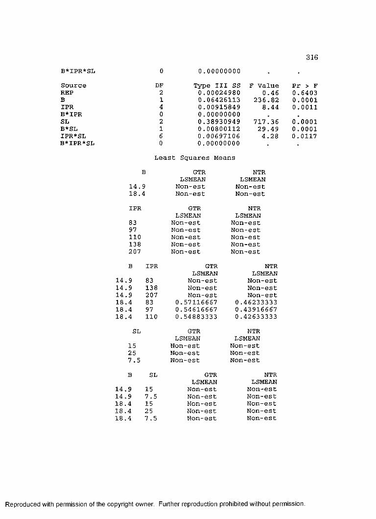
3 1 6
B *IPR*SL 0 0 . 0 0 0 0 0 0 0 0 • •
S o u r c e DF T ype I I I SS F V a l u e P r > FREP 2 0 . 0 0 0 2 4 9 8 0 0 . 4 6 0 . 6 4 0 3B 1 0 . 0 6 4 2 6 1 1 3 2 3 6 . 8 2 0 . 0 0 0 1IPR 4 0 . 0 0 9 1 5 8 4 9 8 . 4 4 0 . 0 0 1 1B*IPR 0 0 . 0 0 0 0 0 0 0 0SL 2 0 . 3 8 9 3 0 9 4 9 7 1 7 . 3 6 0 . 0 0 0 1B*SL 1 0 . 0 0 8 0 0 1 1 2 2 9 . 4 9 0 . 0 0 0 1IPR*SL 6 0 . 0 0 6 9 7 1 0 6 4 . 2 8 0 . 0 1 1 7B *IPR*SL 0 0 . 0 0 0 0 0 0 0 0
L e a s t S q u a r e s M eans
B GTR NTRLSMEAN LSMEAN
1 4 . 9 N o n - e s t N o n - e s t1 8 . 4 N o n - e s t N o n - e s t
IPR GTR NTRLSMEAN LSMEAN
83 N o n - e s t N o n - e s t97 N o n - e s t N o n - e s t110 N o n - e s t N o n - e s t138 N o n - e s t N o n - e s t207 N o n - e s t N o n - e s t
B IPR GTR NTRLSMEAN LSMEAN
1 4 . 9 83 N o n - e s t N o n - e s t1 4 . 9 138 N o n - e s t N o n - e s t1 4 . 9 207 N o n - e s t N o n - e s t1 8 . 4 83 0 . 5 7 1 1 6 6 6 7 0 . 4 6 2 3 3 3 3 31 8 . 4 97 0 . 5 4 6 1 6 6 6 7 0 . 4 3 9 1 6 6 6 71 8 . 4 110 0 . 5 4 8 8 3 3 3 3 0 . 4 2 6 3 3 3 3 3
SL GTR NTRLSMEAN LSMEAN
15 N o n - e s t N o n - e s t25 N o n - e s t N o n - e s t7 . 5 N o n - e s t N o n - e s t
B SL GTR NTRLSMEAN LSMEAN
1 4 . 9 15 N o n - e s t N o n - e s t1 4 . 9 7 . 5 N o n - e s t N o n - e s t1 8 . 4 15 N o n - e s t N o n - e s t1 8 . 4 25 N o n - e s t N o n - e s t1 8 . 4 7 . 5 N o n - e s t N o n - e s t
R eproduced with perm ission of the copyright owner. Further reproduction prohibited without perm ission.

3 1 7
IPR SL GTR NTRLSMEAN LSMEAN
83 15 0 . 5 2 5 1 6 6 6 7 0 . 4 2 0 1 6 6 6 783 2 5 N o n - e s t N o n - e s t83 7 . 5 0 . 3 0 1 6 6 6 6 7 0 . 1 9 3 4 1 6 6 797 15 N o n - e s t N o n - e s t97 25 N o n - e s t N o n - e s t97 7 . 5 N o n - e s t N o n - e s t1 1 0 15 N o n - e s t N o n - e s t11 0 25 N o n - e s t N o n - e s t1 1 0 7 . 5 N o n - e s t N o n - e s t13 8 15 N o n - e s t N o n - e s t1 3 8 7 . 5 N o n - e s t N o n - e s t2 0 7 15 N o n - e s t N o n - e s t2 0 7 7 . 5 N o n - e s t N o n - e s t
B IPR SL GTR NTRLSMEAN LSMEAN
1 4 . 9 83 15 0 . 4 6 8 6 6 6 6 7 0 . 3 6 2 1 6 6 6 71 4 . 9 83 7 . 5 0 . 1 9 0 6 6 6 6 7 0 . 0 7 2 1 6 6 6 71 4 . 9 1 3 8 15 0 . 4 5 0 1 6 6 6 7 0 . 3 0 3 1 6 6 6 71 4 . 9 1 3 8 7 . 5 0 . 2 1 2 6 6 6 6 7 0 . 0 7 0 6 6 6 6 71 4 . 9 2 0 7 15 0 . 4 3 4 6 6 6 6 7 0 . 2 6 0 6 6 6 6 71 4 . 9 2 0 7 7 . 5 0 . 2 4 7 6 6 6 6 7 0 . 0 6 7 6 6 6 6 71 8 . 4 83 15 0 . 5 8 1 6 6 6 6 7 0 . 4 7 8 1 6 6 6 71 8 . 4 83 25 0 . 7 1 9 1 6 6 6 7 0 . 5 9 4 1 6 6 6 71 8 . 4 83 7 . 5 0 . 4 1 2 6 6 6 6 7 0 . 3 1 4 6 6 6 6 71 8 . 4 97 15 0 . 5 4 3 1 6 6 6 7 0 . 4 3 0 1 6 6 6 71 8 . 4 97 25 0 . 6 9 7 1 6 6 6 7 0 . 5 7 8 1 6 6 6 71 8 . 4 97 7 . 5 0 . 3 9 8 1 6 6 6 7 0 . 3 0 9 1 6 6 6 71 8 . 4 110 15 0 . 5 6 9 6 6 6 6 7 0 . 4 4 6 1 6 6 6 71 8 . 4 1 10 25 0 . 7 0 3 6 6 6 6 7 0 . 5 6 9 6 6 6 6 71 8 . 4 110 7 . 5 0 . 3 7 3 1 6 6 6 7 0 . 2 6 3 1 6 6 6 7
------------------------------------------------------- CONS=R-------------------------------------G e n e r a l L i n e a r M o d e ls P r o c e d u r e
C l a s s L e v e l I n f o r m a t i o n
C l a s s L e v e l s v a l u e sB 2 1 4 . 9 1 8 . 4IPR 5 83 97 1 1 0 1 3 8 2 0 7SL 4 15 20 2 5 7 . 5REP 2 1 2
Number o f o b s e r v a t i o n s i n b y g r o u p = 36
D e p e n d e n t V a r i a b l e : GTR
S o u r c eM o d e lE r r o rC o r r e c t e d T o t a l
DF Sum o f S q u a r e s 20 0 . 4 0 9 9 1 0 9 215 0 . 0 0 1 6 8 8 7 235 0 . 4 1 1 5 9 9 6 4
F V a l u e 1 8 2 . 0 5
Pr > F 0 . 0 0 0 1
R eproduced with perm ission of the copyright owner. Further reproduction prohibited without perm ission.

3 1 8
R - S q u a r e C. V. GTR Mean0 , 9 9 5 8 9 7 1 . 7 9 1 7 1 4 0 . 5 9 2 1 9 4 4 4
S o u r c e DF T y p e I SS F V a l u e P r > FREP 1 0 . 0 0 8 9 5 3 5 0 7 9 . 5 3 0 . 0 0 0 1B 1 0 . 0 3 5 7 4 5 4 0 3 1 7 . 5 1 0 . 0 0 0 1IPR 4 0 . 0 0 6 1 5 4 7 2 1 3 . 6 7 0 . 0 0 0 1B *IPR 0 0 . 0 0 0 0 0 0 0 0SL 3 0 . 3 5 2 0 3 1 3 3 1 0 4 2 . 3 0 0 . 0 0 0 1B*SL 2 0 . 0 0 3 3 8 2 6 8 1 5 . 0 2 0 . 0 0 0 3IPR*SL 9 0 . 0 0 3 6 4 3 2 9 3 . 6 0 0 . 0 1 4 1B *IPR *SL 0 0 . 0 0 0 0 0 0 0 0 • •
S o u r c e DF T y p e I I I SS F V a l u e P r > FREP 1 0 . 0 0 1 0 2 3 7 8 9 . 0 9 0 . 0 0 8 7B 1 0 . 0 0 2 8 4 0 7 1 2 5 . 2 3 0 . 0 0 0 2IPR 4 0 . 0 0 2 7 0 1 9 5 6 . 0 0 0 . 0 0 4 3B *IPR 0 0 . 0 0 0 0 0 0 0 0 •
SL 3 0 . 3 2 4 5 1 8 5 2 9 6 0 . 8 4 0 . 0 0 0 1B*SL 2 0 . 0 0 1 4 1 4 1 3 6 . 2 8 0 . 0 1 0 4IPR*SL 9 0 . 0 0 3 6 4 3 2 9 3 . 6 0 0 . 0 1 4 1B*IPR *SL 0 0 . 0 0 0 0 0 0 0 0 ■ •
D e p e n d e n t V a r i a b l e : NTR
S o u r c e DF Sum o f S q u a r e s F V a l u e P r > FM o d e l 20 0 . 4 2 4 6 7 1 3 4 8 1 . 1 1 0 . 0 0 0 1E r r o r 15 0 . 0 0 3 9 2 6 9 7C o r r e c t e d T o t a l 35 0 . 4 2 8 5 9 8 3 1
R - S g u a r e C. V. NTR Mean0 . 9 9 0 8 3 8 3 . 4 1 4 5 3 9 0 . 4 7 3 8 6 1 1 1
S o u r c e DF T y p e I SS F V a l u e P r > FREP 1 0 . 0 1 0 0 4 2 6 7 3 8 . 3 6 0 . 0 0 0 1B 1 0 . 0 8 4 6 7 8 2 5 3 2 3 . 4 5 0 . 0 0 0 1IPR 4 0 . 0 1 3 7 4 5 1 1 1 3 . 1 3 0 . 0 0 0 1B*IPR 0 0 . 0 0 0 0 0 0 0 0 •
SL 3 0 . 3 0 5 4 4 8 1 4 3 8 8 . 9 1 0 . 0 0 0 1B*SL 2 0 . 0 0 2 4 2 2 3 4 4 . 6 3 0 . 0 2 7 2IPR*SL 9 0 . 0 0 8 3 3 4 8 2 3 . 5 4 0 . 0 1 5 1B*IPR *SL 0 0 . 0 0 0 0 0 0 0 0 • •
S o u r c e DF T ype I I I SS F V a l u e P r > FREP 1 0 . 0 0 1 4 7 1 5 3 5 , 6 2 0 . 0 3 1 6B 1 0 . 0 0 5 6 5 2 5 0 2 1 . 5 9 0 . 0 0 0 3IPR 4 0 . 0 2 0 5 3 6 1 0 1 9 . 6 1 0 . 0 0 0 1B *IPR 0 0 . 0 0 0 0 0 0 0 0 .
SL 3 0 . 2 7 8 7 4 6 1 9 3 5 4 . 9 1 0 . 0 0 0 1B*SL 2 0 . 0 0 1 5 5 6 3 4 2 . 9 7 0 . 0 8 1 8IPR*SL 9 0 . 0 0 8 3 3 4 8 2 3 . 5 4 0 . 0 1 5 1B *IPR*SL 0 0 . 0 0 0 0 0 0 0 0 . .
R eproduced with perm ission of the copyright owner. Further reproduction prohibited without perm ission.
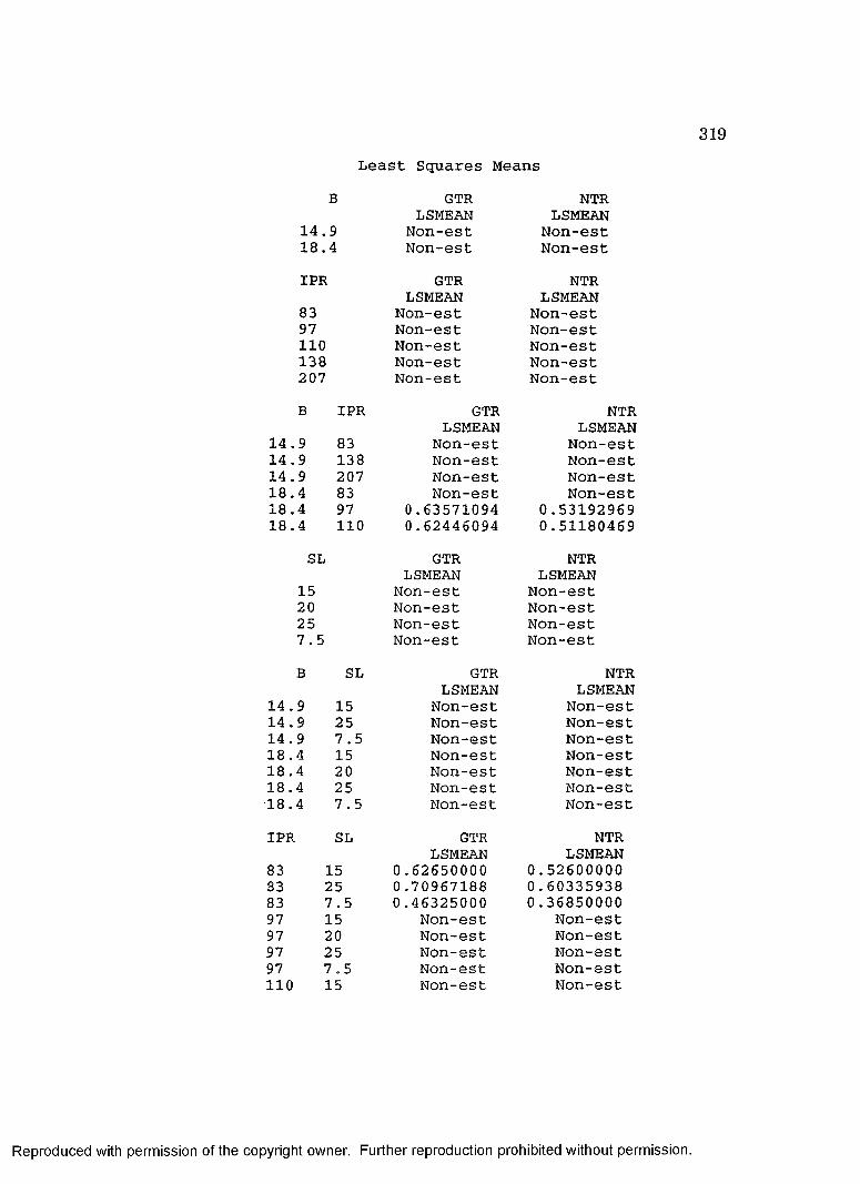
3 1 9
L e a s t S q u a r e s M eans
B GTR NTRLSMEAN LSMEAN
1 4 . 9 N o n - e s t N o n - e s t1 8 . 4 N o n - e s t N o n - e s t
IPR GTR NTRLSMEAN LSMEAN
83 N o n - e s t N o n - e s t97 N o n - e s t N o n - e s t1 10 N o n - e s t N o n - e s t1 3 8 N o n - e s t N o n - e s t207 N o n - e s t N o n - e s t
B IPR GTR NTRLSMEAN LSMEAN
1 4 . 9 83 N o n - e s t N o n - e s t1 4 . 9 13 8 N o n - e s t N o n - e s t1 4 . 9 2 07 N o n - e s t N o n - e s t1 8 . 4 83 N o n - e s t N o n - e s t1 8 . 4 97 0 . 6 3 5 7 1 0 9 4 0 . 5 3 1 9 2 9 6 91 8 . 4 1 10 0 . 6 2 4 4 6 0 9 4 0 . 5 1 1 8 0 4 6 9
SL GTR NTRLSMEAN LSMEAN
15 N o n - e s t N o n - e s t20 N o n - e s t N o n - e s t25 N o n - e s t N o n - e s t7 . 5 N o n - e s t N o n - e s t
B SL GTR NTRLSMEAN LSMEAN
1 4 . 9 15 N o n - e s t N o n - e s t1 4 . 9 25 N o n - e s t N o n - e s t1 4 . 9 7 . 5 N o n - e s t N o n - e s t1 8 . 4 15 N o n - e s t N o n - e s t1 8 . 4 20 N o n - e s t N o n - e s t1 8 . 4 25 N o n - e s t N o n - e s t1 8 . 4 7 . 5 N o n - e s t N o n - e s t
IPR SL GTR NTRLSMEAN LSMEAN
83 15 0 . 6 2 6 5 0 0 0 0 0 . 5 2 6 0 0 0 0 083 25 0 . 7 0 9 6 7 1 8 8 0 . 6 0 3 3 5 9 3 883 7 . 5 0 . 4 6 3 2 5 0 0 0 0 . 3 6 8 5 0 0 0 097 15 N o n - e s t N o n - e s t97 20 N o n - e s t N o n - e s t97 25 N o n - e s t N o n - e s t97 7 . 5 N o n - e s t N o n - e s t1 1 0 15 N o n - e s t N o n - e s t
R eproduced with perm ission of the copyright owner. Further reproduction prohibited without perm ission.

3 2 0
1 1 0 20 N o n - e s t N o n - e s t1 10 25 N o n - e s t N o n - e s t1 10 7 . 5 N o n - e s t N o n - e s t1 3 8 15 N o n - e s t N o n - e s t1 38 25 N o n - e s t N o n - e s t1 38 7 . 5 N o n - e s t N o n - e s t2 07 15 N o n - e s t N o n - e s t2 0 7 25 N o n - e s t N o n - e s t2 0 7 7 . 5 N o n - e s t N o n - e s t
B IPR SL GTR NTRLSMEAN LSMEAN
1 4 . 9 83 15 0 . 6 1 6 5 0 0 0 0 0 . 5 1 0 0 0 0 0 01 4 . 9 83 25 0 . 6 7 5 3 4 3 7 5 0 . 5 6 1 2 1 8 7 51 4 . 9 83 7 . 5 0 . 4 5 7 5 0 0 0 0 0 . 3 5 6 0 0 0 0 01 4 . 9 1 3 8 15 0 . 5 7 1 5 0 0 0 0 0 . 4 7 1 5 0 0 0 01 4 . 9 1 3 8 25 0 . 6 6 6 3 4 3 7 5 0 . 5 2 8 2 1 8 7 51 4 , 9 1 3 8 7 . 5 0 . 4 2 1 5 0 0 0 0 0 . 2 9 2 0 0 0 0 01 4 . 9 2 0 7 15 0 . 5 6 9 5 0 0 0 0 0 . 3 7 6 5 0 0 0 01 4 , 9 2 0 7 25 0 . 6 7 2 5 0 0 0 0 0 . 4 8 9 0 0 0 0 01 4 . 9 2 0 7 7 . 5 0 . 4 7 2 0 0 0 0 0 0 . 3 1 2 5 0 0 0 01 8 . 4 83 15 0 . 6 3 6 5 0 0 0 0 0 . 5 4 2 0 0 0 0 01 8 . 4 83 25 0 . 7 4 4 0 0 0 0 0 0 . 6 4 5 5 0 0 0 01 8 . 4 83 7 . 5 0 . 4 6 9 0 0 0 0 0 0 . 3 8 1 0 0 0 0 01 8 . 4 97 15 0 . 6 3 8 5 0 0 0 0 0 . 5 3 3 0 0 0 0 01 8 . 4 97 20 0 . 6 9 0 3 4 3 7 5 0 . 5 8 6 2 1 8 7 51 8 . 4 97 25 0 . 7 5 1 0 0 0 0 0 0 . 6 3 3 0 0 0 0 01 8 . 4 97 7 . 5 0 . 4 6 3 0 0 0 0 0 0 . 3 7 5 5 0 0 0 01 8 . 4 110 15 0 . 6 1 6 5 0 0 0 0 0 . 5 0 8 0 0 0 0 01 8 . 4 110 20 0 . 6 9 7 3 4 3 7 5 0 . 5 7 3 2 1 8 7 51 8 . 4 110 25 0 . 7 1 7 0 0 0 0 0 0 . 5 9 7 0 0 0 0 01 8 . 4 110 7 . 5 0 . 4 6 7 0 0 0 0 0 0 . 3 6 9 0 0 0 0 0
R eproduced with perm ission of the copyright owner. Further reproduction prohibited without perm ission.

VITA
The author, François P. B rassart was born in 1964 in Cham ps, Aisne,
France. He spent his childhood in Picardy, a region well known for its
agriculture, industry and historical past. G raduated in 1987 from one of
the m ost famous French engineering schools, the Ecole Nationale
Supérieure d’Arts et M étiers (ENSAM), he then earned a M aster of Science
in Agricultural Engineering from Louisiana S tate University in December
1989. The title of his M aster Thesis was; A Computer System to Select
Agricultural Tractor T ires. He also holds a Diploma from the American
Cham ber of Commerce in Paris, showing his in terest in business as well as
engineering.
He lived in various regions of France (North, Picardy, Auvergne, Vosges
and Paris). Being fluent in Spanish and German, besides English, he enjoys
traveling and already visited Belgium, former Yugoslavia, Italy, Canada,
Spain, G uatem ala, Mexico and the U.S.
In 1991, he co-authored a paper he presented during the meeting of the
Society of Automotive Engineers (SAE) in Milwaukee, WI. This paper
presented a research project he had been involved in while studying a t
ENSAM and working with the CEMAGREF, the French National Centre for
Farm Machinery, Agricultural Engineering, W ater and Forestry. The title
of the paper was: ‘Dynamic modeling of the transm ission line of an
agricultural tractor'. In 1993, he presented a second SAE paper he co-
321
R eproduced with perm ission of the copyright owner. Further reproduction prohibited without perm ission.

3 2 2
authored w ith his PhD advisor, Dr. M. E. Wright. The title of th is paper
was: ‘A machine to study vertical tire stiffness and damping coefficient’.
His in terests also include woodwork, gardening, snow-skiing, cycling,
volleyball, soccer and reading. He is a m em ber of several associations:
ENSAM Alumni Association, SAE and ASAE (American Society of
Agricultural Engineers).
R eproduced with perm ission of the copyright owner. Further reproduction prohibited without perm ission.

DOCTORAL EXAM INATION AND D IS S E R T A T IO N REPORT
Candidate:
Major Field:
Title of Dissertation:
Francois Pascal Brassart
Engineering Science
Traction and Agricultural Tractor Tire Selection Studies
Approved:
Major Professor and Chairman
eàn of the Graduate School
EXAMINING COMMITTEE:
; ii.! , /'■
Date of Examination:
Y Û .. r ■ C.
A ':/ ■ /
^luA.^'?''ïïLÂ,Jï
October 25, 1994
R eproduced with perm ission of the copyright owner. Further reproduction prohibited without perm ission.
Recommended