HAL Id: halshs-00464216https://halshs.archives-ouvertes.fr/halshs-00464216
Submitted on 16 Mar 2010
HAL is a multi-disciplinary open accessarchive for the deposit and dissemination of sci-entific research documents, whether they are pub-lished or not. The documents may come fromteaching and research institutions in France orabroad, or from public or private research centers.
L’archive ouverte pluridisciplinaire HAL, estdestinée au dépôt et à la diffusion de documentsscientifiques de niveau recherche, publiés ou non,émanant des établissements d’enseignement et derecherche français ou étrangers, des laboratoirespublics ou privés.
The spread of international financial shocks to AseancountriesCéline Gimet
To cite this version:Céline Gimet. The spread of international financial shocks to Asean countries. Working Paper GATE2009-28. 2009. <halshs-00464216>
DOCUMENTS DE TRAVAIL - WORKING PAPERS
W.P. 09-28
The spread of international financial shocks to Asean countries
Céline Gimet
Décembre 2009
GATE Groupe d’Analyse et de Théorie Économique UMR 5824 du CNRS
93 chemin des Mouilles – 69130 Écully – France B.P. 167 – 69131 Écully Cedex
Tél. +33 (0)4 72 86 60 60 – Fax +33 (0)4 72 86 60 90 Messagerie électronique [email protected]
Serveur Web : www.gate.cnrs.fr
GATE Groupe d’Analyse et de Théorie
Économique UMR 5824 du CNRS
1
The spread of international financial shocks to Asean countries
Céline Gimet1
November 2009
ABSTRACT
This article focuses on the reaction of Asean economies to international financial shocks. The crises in emerging markets at the end of the last century underlined the vulnerability of emerging Asean economies to international financial fluctuations and a lack of sustainability in their exchange rate regime. A Structural VAR model is used to analyze the efficiency of the measures adopted by these countries, after this crisis episode, to protect their economies against speculative attacks. The results reveal that the impact of the current subprime crisis on emerging Asean countries is less significant than that observed in industrialized ones.
JEL Classification: C32, F41, G15.
Keywords: Asean countries, international financial fluctuations, macroeconomic impact, regional integration, SVAR Model.
RÉSUMÉ Cet article se concentre sur la réaction des économies de l'Asean à des chocs financiers internationaux. Les crises qui ont marqué la fin du siècle dernier ont souligné la vulnérabilité des pays émergents de la région à des fluctuations financières internationales ainsi qu’un manque de soutenabilité de leur régime change. Un modèle VAR structurel est utilisé pour analyser l'efficacité des mesures adoptées par ces pays après cet épisode de crise pour protéger leurs économies contre les attaques spéculatives. Les résultats révèlent que l'impact négatif de la crise actuelle sur les pays émergents de l’Asean est moins important que celui observé dans les pays industrialisés.
Classification JEL: C32, F41, G15.
Mots-clés: Asean, fluctuations financières internationales, impact macro-économique, intégration régionale, modèle SVAR.
1 Group for Economic Analysis and Theory (GATE) CNRS UMR 5824- University of Lyon . ENS Lettres et Sciences Humaines-Bureau R132-15 Parvis René Descartes BP 7000 69342 Lyon cedex 07. France. Phone : +33 (0)4 37 37 62 82.Fax : +33 (0)4 37 37 60 24. E-mail : [email protected]
2
1. Introduction
The last decade has been characterized by the development of many trade areas in
Europe (EMU, EU, Cefta), Latin America (Mercosur) and Asia (Asean). During this
period, many emerging countries opened their economy to international trade in order to
benefit from the growth opportunities resulting from economic integration. Today, most
of them have reinforced their commercial and financial links to form common markets,
which correspond to the third stage of the Balassa (1961) classification, and are
attempting to adopt a common currency in order to form a monetary union. The main
problem linked to this type of monetary integration is due to external asymmetric
shocks because the countries have kept their national interest rate and exchange rate as
instruments of adjustment in the event of shocks (Flood, 1979). This problem is
particularly significant in emerging markets (Edwards, 2006). The main condition for
adopting a sustainable monetary union is the ability of the countries to resist these
shocks. Respecting the traditional criteria of the Optimal Currency Areas theory
(Mundell, 1961, McKinnon, 1963, Kenen, 1969) is not sufficient today to protect
countries against exogenous fluctuations. It is important to consider the international
changes that have taken place since this period. More precisely, the recent crises in
emerging markets have underlined the fact that it is important to enlarge the concept of
sustainability: in addition to the lasting stability of economic fundamentals, it is
essential to consider the strength of the country's banking and financial sectors and the
risk of illiquidity in a context of information asymmetry. This would help to avoid
speculative attacks and the spread of financial shocks between countries in the same
block during periods of international crisis (Corsetti and al., 1999, Chang and al.,
2000). But the numerous financial crises that occurred in emerging markets at the end of
the last century - in Asia in 1997-1998, in Latin America in 1994, 1999 and 2001 and in

3
Eastern Europe in 1998 and 2001 - have highlighted the inability of these countries to
adopt this common exchange rate solution. In general, the crisis had harmful effects on
all the countries of the region where it occurred and sometimes infected more distant
regions. For example, a “fast and furious” episode of contagion followed the Thai crisis
(Kaminsky and al., 2003) and most emerging countries of the area that adopted a fixed
or quasi-fixed exchange rate were forced to let their currency float.
But, today, it seems that emerging markets have learned some lessons from these
crises and have reinforced their structures to protect their banking and financial sectors
from international fluctuations and speculative attacks. In fact, the subprime crisis,
which originated in the United States in July 2007, seems to have had spillover effects
on the banking and financial sectors of Western European countries and Japan and less
significant impact on emerging markets. Therefore, it is extremely interesting to analyze
the different effects of these crises on countries in a commercial area according to their
economic characteristics (industrialized or emerging) and during different crisis
episodes. More precisely, the purpose of this article is to underline the progress of the
emerging countries since the nineties crisis episode and their capacity to resist the
subprime crisis and to draw some conclusions concerning their ability to adopt, in the
future, a monetary union. The study concentrates on the case of the Asean (Association
of Southeast Asian Nations) +3 countries2. Two reasons justify this choice. Firstly, this
is one of the regions most hit by financial crises at the end of the last decade; it is
interesting to analyze the evolution of the different countries in their ability to stabilize
their banking and financial sectors in order to guarantee the confidence of international
4
lenders. Secondly, this commercial block is made up of industrialized and emerging
economies; therefore it is important to compare the strength and the duration of the
shock resulting from different crisis episodes according to these countries' economic
characteristics.
Many econometric instruments can be used to measure the vulnerability of countries
to an external shock; in particular Vector Auto-Regression (VAR) models (Calvo and
al., 2000; Bordo and al., 2006). But Structural Auto-Regression methodology (SVAR)
seems to be more accurate because it makes it possible to impose identifying restrictions
on relationships between the model's variables, in reference to the economic theory; it
enables one to include real and nominal variables and ensures a better interpretation of
results.
A second section deals with the choice of the method, sample and variables used in
our analysis. In a third section, the results obtained are analyzed. In a fourth section, the
similarities between the countries are underlined thanks to a correlation test concerning
their responses to a common shock. A group of countries that have a close economic and
financial profile and consequently the same reaction to a common shock is identified
before concluding.
2. An empirical analysis
2.1. The structural VAR model
2 Brunei Darussalam (1984), Cambodia (1999), Indonesia (1967), Laos (1997), Malaysia (1967), Myanmar
(1997), Philippines (1967), Singapore (1967), Thailand (1967), Vietnam (1995) + China, Japan and South
Korea (1997).
5
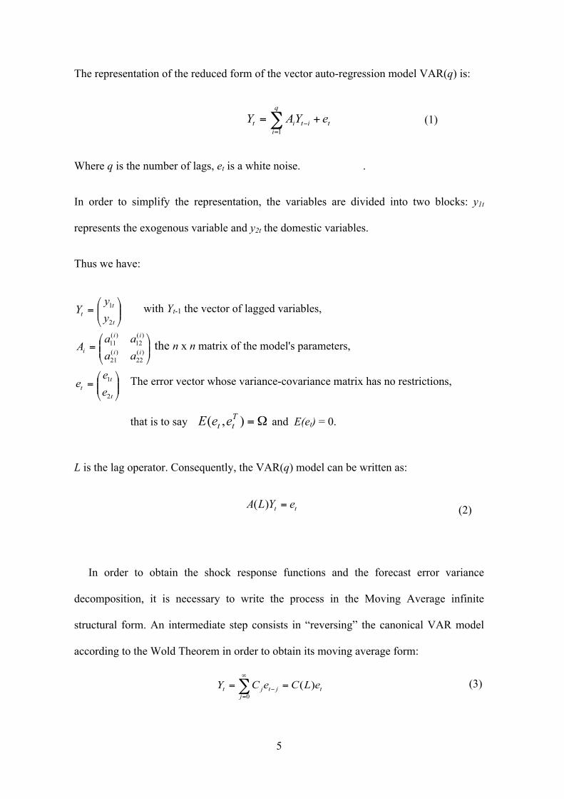
The representation of the reduced form of the vector auto-regression model VAR(q) is:
(1)
Where q is the number of lags, et is a white noise. .
In order to simplify the representation, the variables are divided into two blocks: y1t
represents the exogenous variable and y2t the domestic variables.
Thus we have:
L is the lag operator. Consequently, the VAR(q) model can be written as:
(2)
In order to obtain the shock response functions and the forecast error variance
decomposition, it is necessary to write the process in the Moving Average infinite
structural form. An intermediate step consists in “reversing” the canonical VAR model
according to the Wold Theorem in order to obtain its moving average form:
(3)
with Yt-1 the vector of lagged variables,
the n x n matrix of the model's parameters,
The error vector whose variance-covariance matrix has no restrictions,
that is to say and E(et) = 0.

6
where et represents the vector of canonical innovations.
Thus, the structural Moving Average representation is:
(4)
with (5)
where P is an invertible matrix n x n which has to be estimated in order to identify the
structural shocks. The short-run constraints are imposed directly on P and correspond to
some elements of the matrix set to zero. The Θj matrix represents the response functions
to shocks εt of the elements of Yt. The different structural shocks are supposed to be non-
correlated and to have a unitary variance:
(6)
Ω is the variance-covariance matrix of the canonical innovations et, thus :
(7)
2.2. The choice of variable
(5)

7
Our study is based on Asean+3 countries3 for the period 1990M1-2009M7. This is
divided into two sub-periods4 which correspond to the two main crisis episodes which hit
Asean countries: the Thai crisis in 1997-1998 and the subprime crisis in 2007-2009. For
each crisis episode, the purpose is to measure the reaction of Asean countries to this
international disturbance and to make comparisons between the periods and the countries.
The variables are selected so as to see the impact of the international financial shock
on the countries' economic, monetary and financial sectors. If it hits only the financial
sphere and involves only a small outflow of capital, we can conclude that the harmful
consequences of the international disturbance are limited. But, if the shock is propagated
into the real sector and induces a reaction of the monetary authorities in order to stabilize
the economies, all sectors are weakened and the time necessary to eliminate the negative
impact of the crisis is going to be long.
In our model, each Asean economy is described by the following vector of
endogenous variables:
The external disturbances (external) retained to represent the different episodes of
volatility are a positive shock of emerging markets' composite stock exchange index
3 Because of the availability of data our sample is only made up of 8 countries: Indonesia, Malaysia, the
Philippines, Singapore, Thailand, China, Japan and South Korea.
4 1990M1-1999M12 and 2000M1-2009M7.
8
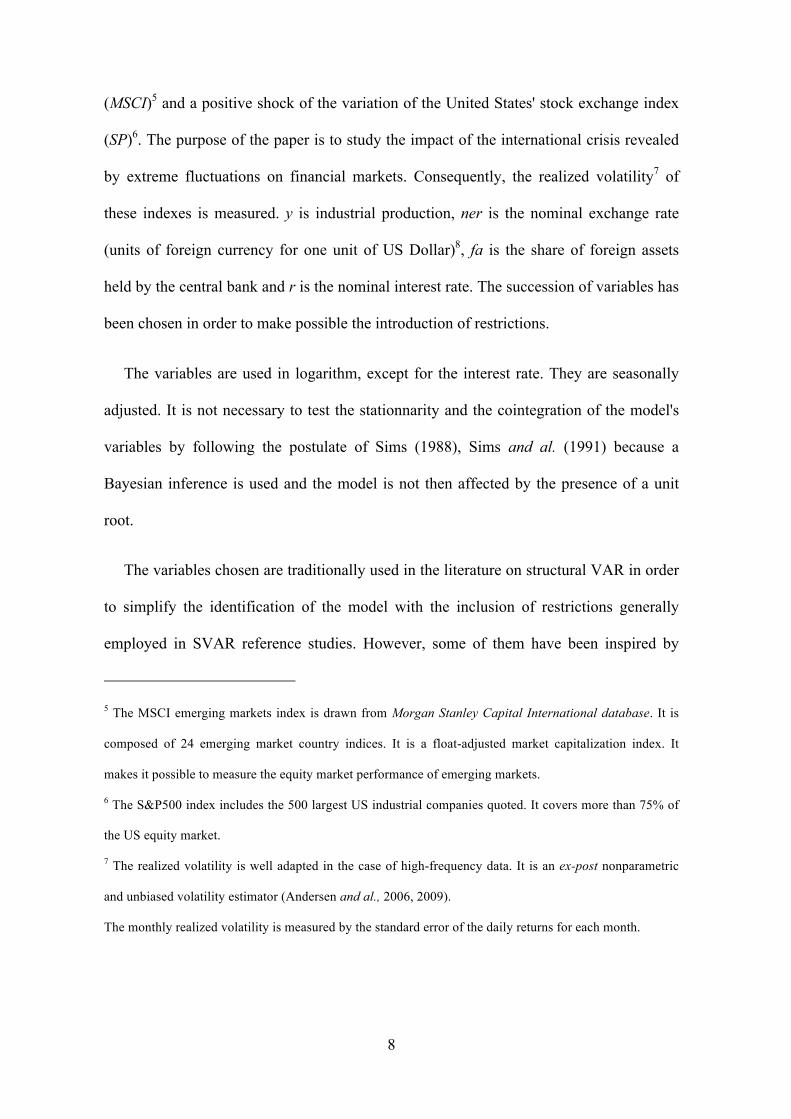
(MSCI)5 and a positive shock of the variation of the United States' stock exchange index
(SP)6. The purpose of the paper is to study the impact of the international crisis revealed
by extreme fluctuations on financial markets. Consequently, the realized volatility7 of
these indexes is measured. y is industrial production, ner is the nominal exchange rate
(units of foreign currency for one unit of US Dollar)8, fa is the share of foreign assets
held by the central bank and r is the nominal interest rate. The succession of variables has
been chosen in order to make possible the introduction of restrictions.
The variables are used in logarithm, except for the interest rate. They are seasonally
adjusted. It is not necessary to test the stationnarity and the cointegration of the model's
variables by following the postulate of Sims (1988), Sims and al. (1991) because a
Bayesian inference is used and the model is not then affected by the presence of a unit
root.
The variables chosen are traditionally used in the literature on structural VAR in order
to simplify the identification of the model with the inclusion of restrictions generally
employed in SVAR reference studies. However, some of them have been inspired by
5 The MSCI emerging markets index is drawn from Morgan Stanley Capital International database. It is
composed of 24 emerging market country indices. It is a float-adjusted market capitalization index. It
makes it possible to measure the equity market performance of emerging markets.
6 The S&P500 index includes the 500 largest US industrial companies quoted. It covers more than 75% of
the US equity market.
7 The realized volatility is well adapted in the case of high-frequency data. It is an ex-post nonparametric
and unbiased volatility estimator (Andersen and al., 2006, 2009).
The monthly realized volatility is measured by the standard error of the daily returns for each month.

9
recent financial crisis theory. Thus, the variables y, ner and r can be found in studies
concerning the impact of monetary fluctuations on economic cycles which underline the
role of the exchange rate in the spread of the shock (Cushman and al., 1997, Kim and al.,
2000, Canova, 2005, Mackowiak, 2007). The decomposition between supply and demand
shocks follows the postulate of Gali (1992), Cushman and al. (1997) which is based on
an ISLM model. Moreover, the literature on the “third generation of crisis” has recently
underlined the necessity of considering the country's illiquidity risk in the spread of the
crisis and thus, the role of international reserves in a national economy (Corsetti and al.,
1999, Chang and al., 2000). Finally, the importance of taking into account the
vulnerability of emerging markets to international fluctuations has been demonstrated by
Canova (2005), Mackowiak (2007).
The originality in this analysis is the inclusion of the two variables of stock exchange
volatility. This choice is inspired by the recent mechanism of financial contagion during
crisis episodes in economies whose banking system is vulnerable and illiquidity risk
significant. Even if the origins of the crisis are different (the 1997 Asian crisis started on
the foreign exchange markets and the 2008 subprime crisis began in the housing sectors)
the consequences are identical. The shock causes considerable stock exchange volatility.
And international lenders' loss of confidence after a crisis in a country can generate a
portfolio reallocation on the behalf of these investors in order to limit their exposure to
risk. This situation creates a considerable outflow of capital from economies which have
the same characteristics as the first country hit by the crisis (Calvo, 1999, Kaminsky and
al., 1999, Kodres and al., 2002). International reserves decrease and the monetary
8 It can be noticed that we use a Bayesian inference. So, in this case, it is not necessary to test the
stationnarity and the cointegration of the model's variables by following the postulate of Sims (1988), Sims
10
authority may increase the interest rate which can produce a reduction in economic
growth.
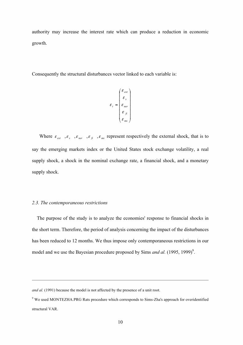
Consequently the structural disturbances vector linked to each variable is:
Where represent respectively the external shock, that is to
say the emerging markets index or the United States stock exchange volatility, a real
supply shock, a shock in the nominal exchange rate, a financial shock, and a monetary
supply shock.
2.3. The contemporaneous restrictions
The purpose of the study is to analyze the economies' response to financial shocks in
the short term. Therefore, the period of analysis concerning the impact of the disturbances
has been reduced to 12 months. We thus impose only contemporaneous restrictions in our
model and we use the Bayesian procedure proposed by Sims and al. (1995, 1999)9.
and al. (1991) because the model is not affected by the presence of a unit root.
9 We used MONTEZHA.PRG Rats procedure which corresponds to Sims-Zha's approach for overidentified
structural VAR.
11
Our objective is to identify the n² elements of the P matrix. The Ω matrix is symmetric,
consequently n(n+1)/2 orthogonalization constraints are already imposed. It is necessary
to determine the n(n-1)/2 remaining constraints; we have chosen to impose 11 short term
restrictions in reference to the economic literature, thus the model is over-identified.
Firstly, we consider the external variables (MSCI and SP) to be exogenous (Cushman
and al., 1997, Mackowiak, 2007). Secondly, we follow the postulate of the authors who
believed that the monetary authority's function of reaction, that is to say the interest rate,
does not react immediately to a shock in price and production. Then we suppose that the
monetary policy's response to these shocks and to financial disturbances10 is postponed
for a month because of information delay (Sims and al., 1995, 1999, Kim and al., 2000).
Finally, the hypothesis of a lag in the response of economic activity to international and
national financial disturbances and to monetary shock is retained (Kim and al., 2000).
Thus:
Following the information criteria of Schwartz, Akaike and Hannan-Quinn, four lags
have been retained for all models and complementary tests underlined the absence of
autocorrelation in the residuals11
The model is now identified. We can report, in the following section, the empirical
results.
10 National and international.
11 Detailed information concerning the tests and their results is available on request.
12
3. The results
The countries' exchange rate regime is an important parameter to take into
consideration as it influences the orientation of economic policies and subsequently their
responses to a common shock. Over the periods of analysis, according to a de facto
classification12, China is the only country which maintained a perfect fixed exchange rate
with a peg to US Dollar until 2005 and then adopted a crawling peg. Some countries of
the region experienced an intermediate regime before 1997 (Indonesia, Malaysia and
Thailand) but, except for Malaysia, they were obliged to let their currency float after the
Asian crisis. The other countries of the region have either made independent or managed
floating regimes since 1990 (Japan, Korea, Philippines and Singapore). However, it is
important to note that during the second period of analysis, Japan and Singapore are the
only countries in the sample which have not used inflation or a monetary target.
We can suppose that the economies' responses to a common financial shock were
divergent in the first period of analysis; many economic differences existed between
developed and emerging countries and they had diverse exchange rate regimes. But after
the Asian crisis, we can expect a better convergence in the countries' reaction for three
main reasons. Firstly, most of them have adopted a floating regime. Secondly, most of
them have been harmed by the Asian crisis and have taken different measures to protect
their economy against short term capital flows. Finally, all of them have decided to
cooperate in order to reduce the risk of financial crisis with the implementation of the
12 Bubula, A., Ötker-Robe, I., 2002, “The evolution of Exchange Rate Regimes since 1990: Evidence from
De Facto Policies”, IMF Working Paper, 155.
IMF, Annual Report on Exchange Arrangements and Exchange Restrictions, 1990-2008.

13
Chang Mai Initiative13. The main objective is to reinforce regional financial surveillance
and to develop assistance mechanisms in the event of financial difficulties and lack of
liquidities in one of the countries of the region (development of bilateral swaps and
repurchase agreement facilities in addition to the expansion of the ASEAN regional Swap
Arrangement). Moreover, the financial integration of the Asean+3 countries was
strengthened in 2003 with the Asian Bond Market Initiative which aims to develop
regional liquid bond markets.
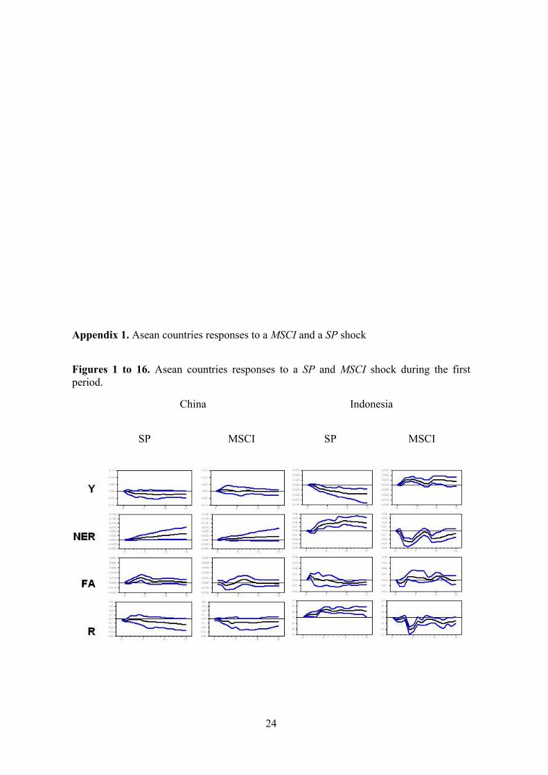
The graphics, in appendix 1, show the reaction of domestic variables after a one-
standard-deviation positive variation of the external variable. They reveal the significance
level of the results if the interval of confidence does not include the 0 axis.
3.1. The vulnerability of Asean economies at the end of the last century
First of all, we concentrate on the period 1990M1-1999M12 and we study the
responses of Asean economies to a volatility shock on MSCI and SP (Appendix 1, figures
1 to 16). Overall, the results underline the considerable vulnerability of emerging Asean
countries to the SP shock. This phenomenon can be explained by the fact that the
countries' exchange rates were linked to the US Dollar. Moreover, during this first period
of analysis, there was a particularly strong influence of the US stock market in the global
financial system (Kim and al., 2009).
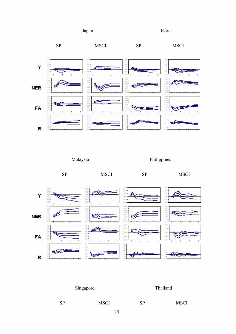
The reaction of the countries converges. However, the impact of the SP shock is more
pronounced in emerging ones. This shock generates an immediate loss in international
investors’ confidence, particularly significant in Thailand, Korea and Malaysia which
experienced a large capital outflow (fa). In the developed countries the reaction of this
13 May 6, 2000, Chiang Mai, Thailand.
14
variable is less significant because, in the nineties, they were the developing Asean
economies' main creditors; in order to limit their exposure to risk on international markets
they massively removed their investments in short-term capitals from these countries and
did not experience an outflow of capital. Similarly, the impact on China’s capital flows is
not significant because, during the nineties, the financial openness of the country was
limited and the flows of international reserves controlled.
This phenomenon is at the origin of a depreciation of the nominal exchange rate in the
short term in all emerging countries of the region (ner), except China whose exchange
rate stayed pegged to the US Dollar. We can notice a slight devaluation in the medium
term in Singapore, which can be explained by an intervention of the Monetary Authority
in this direction. Moreover, in the short term, Japan which exported 40% of its products
to Asean countries experienced a short decrease in its growth rate and a temporary
depreciation of its currency. But it was one of the world's largest holders of currency
reserves at the time and the situation was quickly rectified.
In order to limit the negative effects of this shock, the central bank of all countries in the
region increased the nominal interest rate during the first months following the crisis (r).
On this point, a slight difference exists between countries with fixed and floating
exchange rates. The countries dependent on the United States' monetary policy
experienced a less pronounced variation in their interest rate. They were influenced by
the decrease in the US interest rate aimed at stimulating domestic economic growth.
Finally, the increase in the interest rate level and/or the decrease of international reserves
in the countries were at the origin of a decline in production in the entire region, more
pronounced in emerging markets (y).

15
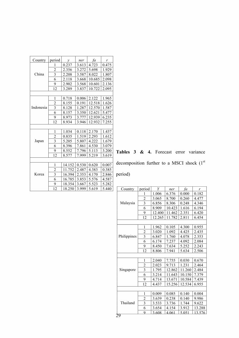
During the same period, the countries' reactions to an MSCI shock are quite different
except for Korea. The more industrialized countries (Japan and Singapore) and China
were not significantly impacted by this shock. In the other countries, we note an outflow
of international reserves revealing the investors’ loss of confidence (fa). This situation
generates a devaluation of the nominal exchange rate (ner) less pronounced than those
produced by an SP shock. But the main difference lies in the response of the nominal
interest rate (r) which decreases in emerging Asean countries in order to boost economic
growth (y) (particularly in Thailand, Malaysia and Indonesia). This situation can be
linked to less variation in capital outflows.
During this period, volatility shocks explain more than 10% of the variation in
international reserves in the year following the shock. Moreover, they were at the origin
of nearly 10% of production variation in most countries of the region (appendix 2, tables
1 and 2). All the region's emerging countries were hit by the shock. It spread from the
financial to the real sector of the economy. This underlines the vulnerability of emerging
Asean countries to international fluctuations during the nineties and their incapacity to
limit the negative consequences. This situation was due to their early capital account
openness, at the beginning of the century, followed by excessive risk-taking, which is
shown by the banking and financial indicators’ deterioration during the four years
preceding the Thai crisis. To be more precise, the situation of the banking and financial
sectors in Asean countries worsened after 1994 because of a large decrease in banking
liquidities and a rise in short-term debt, increasing the total amount of external debt
which was responsible for international lenders' loss of confidence (Corsetti and al.,
1999, Chang and al., 2000, Gimet, 2007). Our results demonstrate a spread of the crisis in
all the region's emerging countries that corresponds to the “Fast and Furious” episode of
contagion defined by Kaminsky and al. (2003).
16
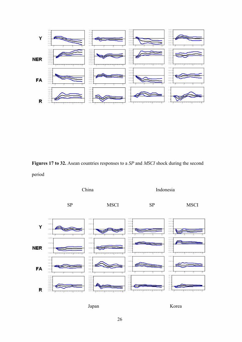
3.2. The impact of the subprime crisis in Asean countries
Secondly, we analyze the impact of the subprime crisis in the same economies
(Appendix 1, figures 17 to 32). A volatility shock seems to have many different effects on
these economies. These divergences cannot be explained by the exchange rate regime
because all these countries, except China, have a free or managed floating exchange rate
regime. However, the emerging Asean countries less dependent on the United States have
been more vulnerable to an MSCI shock (appendix 2, table 4) due to their more
pronounced economic and to a certain extent financial integration with the countries of
the block and the other emerging markets (Kim and al., 2009)..
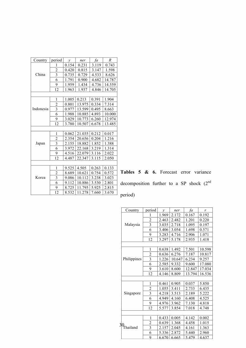
After an SP shock, the countries which suffer from a significant inflow of capitals
are the developed ones (fa). China has experienced capital flow volatility due to the
gradual deregulation of its financial markets. Thailand and Indonesia have seen their
international reserves decrease but only in the short run. Consequently, the impact on the
other macroeconomic and financial variables is reduced in comparison to the last crisis
episode in all emerging countries: the nominal exchange rate does not fluctuate
significantly (ner) and the impact on production is limited (Malaysia, Korea, Indonesia),
or not significant (Philippines, Thailand) (y). Thus, the monetary policy does not react
massively. On the other hand, we note action on the interest rate by Singapore's central
banks (r) and a pronounced decrease in production in Japan, Singapore and China.
Finally, the crisis is at the origin of more significant volatility in these countries'
exchange rate except in China which has maintained its crawling peg.
The reactions of the Japanese economy to an MSCI shock are equivalent to those
of an SP shock. The country has experienced an outflow of capital and a reduction in its
production. Similarly, China's growth has been reduced (y). Symmetrically, some

17
emerging markets (the Philippines, Thailand) that have not been vulnerable to an SP
shock have not been impacted by an MSCI shock. However, we notice a small outflow of
capital (fa) in Korea, Malaysia and Indonesia followed by a short devaluation of the
nominal exchange rate (ner) and a slight increase in the interest rate (r) which contribute
to a decrease of growth (y). Even if these countries' responses are less marked than during
the first crisis episode, the economy's behavior reveals some weaknesses.
Thus when we compare these results with those of the previous period of analysis, we
can make many comments. Firstly, the main differences in the countries' reaction can be
explained by several factors. To begin with, the situation has changed at an international
level. In recent years, international reserves have been concentrated in emerging countries
which have become the new international lenders (in particular in China and OPEC
countries) and the most developed economies, the new creditors. This situation explains
these markets' greater vulnerability. Moreover, some emerging Asean countries which
experienced the very negative impacts of their last crisis have decided to adopt prudential
measures in order to protect their economies against speculative attacks and reduce their
vulnerability to international financial shocks. More precisely, they have limited short-
term capital inflows and consolidated their banking sector. Then, even if the amount of
international flows of capitals in emerging markets has been more important than those in
the first period of analysis (the region14’s gross external assets and liabilities has gained
57 points of GDP from 1990 to 2006, Kim and al., 2009), the macroeconomics impacts
were lower. Our analysis reveals the efficiency of these measures, in particular in
Thailand and the Philippines. But some progress would be necessary in order to protect
the entire region against these financial fluctuations for certain emerging countries
14 Japan excluded.

18
(Korea, Malaysia and Indonesia) were still experiencing difficulties during the second
period of analysis.
4. The similarities in responses to a common shock
In order to compare the countries' reactions to each common shock, we propose an
analysis of the correlation of the Asean economies' significant responses during the year
following the shock (Appendix 3).
Symmetry in the countries' reaction and the economies' low vulnerability reveal a
structural economic and financial convergence of these economies towards sustainable
levels that guarantees international lenders' confidence.
For the first crisis episode, our results show a convergence in the response of all the
domestic variables of Indonesia, Korea, the Philippines, Malaysia and Thailand to a
common SP volatility shock (table 5). In particular, the outflow of capital (fa) is very
strong in these five countries. All the countries were forced to devaluate their exchange
rate, except Japan where this devaluation was limited. The evolution of the variable ner is
then correlated between most countries in the region. The reaction of the monetary
authorities (r) was quite similar between countries, except for China which fixed its
exchange rate and Japan that experienced a nominal interest rate at a low level. The crisis
spread in the real sector and generated a reduction in production (y) in all the countries of
the region, in particular the emerging ones.
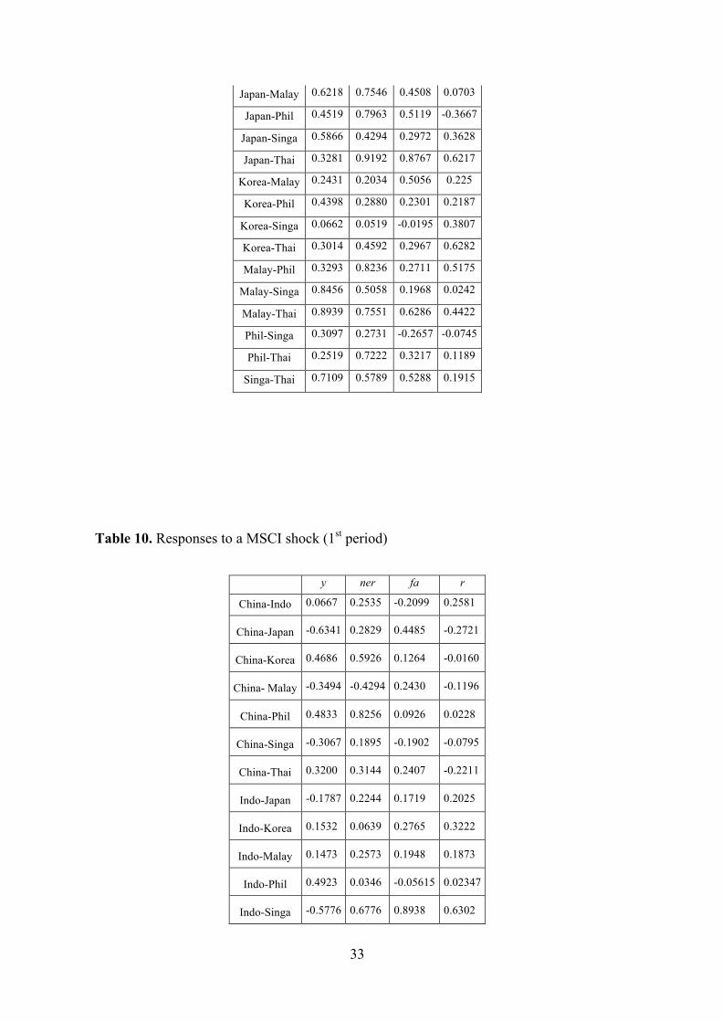
Some variables, like the interest rate, did not have the same evolution after an MSCI
shock and thus the impact on the production is different. We can note a less important
correlation in the emerging Asean economies' responses, in particular for Korea. Japan
and Singapore were less vulnerable to this shock.

19
We can conclude that emerging markets were the most vulnerable to the financial shock
during this crisis episode, in particular to the SP shock. The convergence in their
reactions underlines the fact that, whatever the size and the exchange rate regime of these
economies, they were hit by the crisis which spread from the financial to the real sector.
Their intermediate exchange rate regimes were not sustainable. On the other hand, the
financial and real impacts in industrialized countries are limited. China was an exception
because its financial and economic openness was weak during this period. Thus, the
reaction of its domestic variables is less correlated with the other Asean countries.
Moreover, the disparity in the responses to MSCI shocks underlines the lack of structural
convergence in the region during this period.
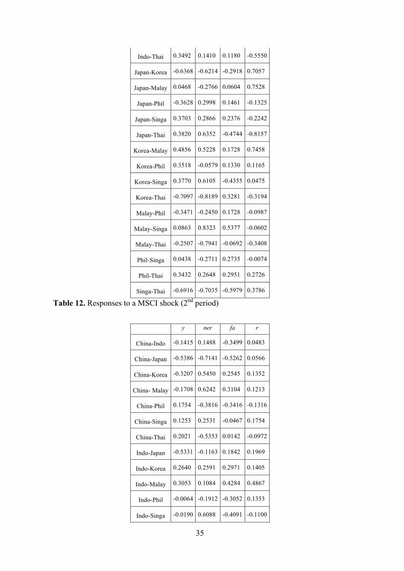
For the current crisis, our results are different from those of the previous period of
analysis (table 6). We can note similarities in the reaction of industrialized countries, in
particular Japan and Singapore, which experience an outflow of assets (fa) after a shock
in SP and MSCI. At the same time, their exchange rate (ner) and their production (y)
move in a similar direction.
The responses of the domestic variables of Indonesia, Korea and Malaysia are quite
similar but these countries are less vulnerable and their reactions to international shocks
are more limited than in the previous period of analysis. The main negative impact in
these three economies is on production. The Philippines and Thailand do not react
significantly to these shocks.
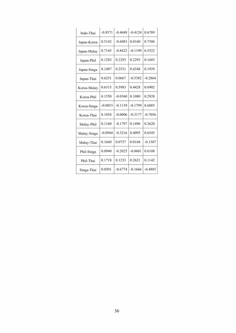
China maintains its crawling peg and its responses to the common financial shock are
different from those of other countries in the region, except regarding its interest rate.
We can thus conclude that the most industrialized countries are those most harmed by the
crisis which spreads in the real sector of their economy. Moreover, a group of countries
20
formed by the Philippines and Thailand, which were the countries most vulnerable to the
Thai crisis, have made significant progress in protecting their economy against
international financial shock and in reinforcing their structural convergence. But many
disparities still exist between the countries of the region and greater structural
convergence is necessary in order to deepen their integration and envisage a monetary
union.
5. Conclusion
Our results highlight the negative impact of the financial crisis in emerging Asean
economies at the end of the last century. They were very vulnerable to international
financial fluctuations because their growth depended mainly on the confidence of
international lenders who invested a considerable amount of short term capital in these
economies. This situation reveals the inability of emerging Asean countries to prevent
and absorb these types of shocks during this period. The fact that all the region's
emerging economies were hit by the crisis shows that the exchange rate regimes in place
during this period were not sustainable.
But the comparison of these results with those from the second period of analysis
allows us to observe several significant differences. In fact the recent stock exchange
volatility seems to have had limited impacts on certain emerging Asean countries. On the
other hand, the negative effects are more significant in industrialized ones, including
China. We can conclude that the measures adopted by the emerging Asean economies at
the beginning of this decade have been very efficient. They decided to limit their
dependence on short-term capital flows, to reduce the risk of illiquidity of their economy
and to consolidate their banking sector. These actions have made it possible, to a certain
extent, to maintain international lenders' confidence in a period of international

21
fluctuations and thus to limit capital outflows. Today, a group of emerging markets
constituted by the Phillipines, Thailand and, to a certain extent, Malaysia, Indonesia and
Korea, has made significant progress in improving its capacity to limit the negative
impact of international financial fluctuations. Moreover, the similarities in the responses
of the Phillipines and Thailand to a common shock highlight a better structural financial
convergence between them and towards a sustainable level.
We can conclude that the recent financial crisis has spread in the most advanced
countries directly through the financial channel which includes both banking exchanges
between the countries and variations in financial assets. The crisis has extended from the
financial to the real sector in these countries. Thus, the fundamental contagion of the
crisis in emerging markets is indirect and is propagated through the real channel of trade
links between them and industrialized countries.
22
References
Andersen TG, Bollerslev T, Diebold FX 2009. Parametric and Nonparametric Volatility Measurement. In: Aït-Sahalia Y, Hansen LP (Eds), Handbook of Financial Econometrics Elsevier, vol. 1.1.
Andersen TG; Bollerslev T., 2006. Realized return volatility, asset pricing, and risk management. NBER Reporter.
Balassa B., 1961. The Theory of Economic Integration. Irwin, Homewood, Illinois. Bordo MD, Murshid AP, 2006. Globalization and changing patterns in the international transmission of shocks in financial markets. Journal of International Money and Finance; 25; 655-574. Calvo GA, Mendoza EG, 2000. Rational herd behavior and the globalization of securities markets. Journal of International Economics; 51; 79-113. Canova F., 2005. The transmission of US shocks to Latin America. Journal of Applied Econometrics; 20; 229-251. Chang R, Velasco A., 2000. Banks, debt maturity and financial crises. Journal of International Economics; 51; 169-194. Corsetti G, Pesenti P, Roubini N., 1999. Paper tigers? A model of the Asian crisis. European Economic Review; 43; 1211-1236. Cushman DO, Zha T., 1997. Identifying monetary policy in small open economy under flexible exchange rate. Journal of Monetary Economics; 39; 433-448.

23
Edwards S., 2006. Monetary unions, external shocks and economic performance: A Latin American perspective. International Economics and Economic Policy; 3; 225-247. Flood RP, 1979. Capital mobility and the choice of exchange rate system. International Economic Review; 2; 405-416. Gali J., 1992. Does the IS-LM model fit us postwar data?. Quarterly Journal of Economics; CVII; 708-738. Gimet C., 2007. Conditions necessary for the sustainability of an emerging area: the importance of banking and financial regional criteria. Journal of Multinational Financial Management; 17; 317-335. Kaminsky GL, Reinhart C, Vegh CA, 2003. The unholy trinity of financial contagion. Journal of Economic Perspectives; 17; 51-74. Kenen P., 1969. The Theory of Optimum Currency Areas: an Eclectic View. In: Mundell RA, Swoboda AK (Eds), Monetary Problems in International Economy, Chicago University Press. Kim S, Roubini N., 2000. Exchange rate anomalies in the industrialized countries: A solution with a Structural VAR approach. Journal of Monetary Economics; 45; 561-586. Kim S, Lee JW, Park, CY, 2009. Emerging Asia: Decoupling or Recoupling. Working Papers on Regional Economic Integration; 31; Asian Development Bank. Mackowiak B., 2007. External shocks, US monetary policy and macroeconomic fluctuations in emerging markets. Journal of Monetary Economics; 54; 2512-2520. McKinnon R., 1963. Optimum currency areas. American Economic Review; 53; 717-725. Mundell RA, 1961. A theory of optimum currency areas. American Economic Review; 51; 509-517. Sims CA, 1988. Bayesian skepticism on unit root econometrics. Journal of Economic Dynamics and Control; 12; 463-474. Sims CA, Uhlig H, 1991. Understanding Unit Rooters: a Helicopter Tour. Econometrica; 59; 1591-1599. Sims CA, Zha, T., 1995. Does monetary policy generate recessions? : Using less aggregate price data to identify monetary policy. Working paper, Yale University, CT. Sims CA, Zha, T., 1999. Error bands for impulse responses. Econometrica; 67; 1113-1155.
24
Appendix 1. Asean countries responses to a MSCI and a SP shock
Figures 1 to 16. Asean countries responses to a SP and MSCI shock during the first period.
China Indonesia
SP MSCI SP MSCI
25
Japan Korea
SP MSCI SP MSCI
Malaysia Philippines
SP MSCI SP MSCI
Singapore Thailand
SP MSCI SP MSCI
26
Figures 17 to 32. Asean countries responses to a SP and MSCI shock during the second
period
China Indonesia
SP MSCI SP MSCI
Japan Korea

27
SP MSCI SP MSCI
Malaysia Philippines
SP MSCI SP MSCI
Singapore Thailand
SP MSCI SP MSCI

28
Appendix 2. Forecast error variance decomposition further to a MSCI and a SP shock
Tables 1 & 2. Forecast error variance decomposition further to a SP shock (1st period)
Country period y ner fa r 1 1.290 0.067 3.427 10.004 2 3.912 0.261 5.473 9.081 3 4.697 0.280 8.192 8.349 6 7.890 4.721 8.262 8.303 9 7.823 6.340 8.338 8.716
Malaysia
12 8.662 6.733 8.226 8.653
1 1.359 0.993 5.879 1.946 2 2.196 2.753 7.168 1.792 3 4.656 3.429 7.038 3.289 6 11.695 8.339 9.086 3.583 9 12.939 10.972 9.226 3.341
Philippines
12 12.333 11.678 9.245 3.600
1 1.596 0.269 14.686 0.291 2 1.413 0.635 14.723 1.124 3 4.839 1.631 14.331 1.941 6 4.988 6.777 18.345 2.562 9 4.927 6.717 19.625 2.637
Singapore
12 6.166 7.456 19.460 2.988
1 1.794 0.219 0.047 5.037 2 8.599 0.425 9.005 4.126 3 9.150 1.222 9.209 4.486 6 9.207 1.522 9.165 12.565 9 9.180 2.596 8.812 14.249
Thailand
12 9.173 2.679 8.880 14.443
29
Tables 3 & 4. Forecast error variance
decomposition further to a MSCI shock (1st
period)
Country period y ner fa r 1 0.237 3.613 4.723 0.475 2 2.356 3.272 5.698 1.929 3 2.208 3.587 8.022 1.807 6 2.118 3.668 10.685 2.098 9 2.902 3.568 10.601 2.136
China
12 3.289 3.837 10.722 2.095
1 0.718 0.006 2.122 1.965 2 8.155 0.191 12.518 1.626 3 8.128 1.287 12.570 1.587 6 8.157 3.350 12.621 5.477 9 8.973 3.777 12.939 6.235
Indonesia
12 8.934 3.946 12.932 7.255
1 1.034 0.118 2.170 1.437 2 0.835 1.519 2.293 1.612 3 5.205 5.807 4.222 1.679 6 8.396 7.861 4.530 3.079 9 8.552 7.796 5.113 3.200
Japan
12 8.577 7.999 5.219 3.619
1 14.152 0.530 0.620 0.007 2 11.752 2.487 4.383 0.385 3 16.394 2.353 4.170 2.846 6 16.785 3.853 5.576 4.587 9 18.354 3.667 5.523 5.282
Korea
12 18.250 3.999 5.619 5.440
Country period Y ner fa r 1 1.006 6.376 0.000 0.182 2 3.065 8.700 0.260 4.477 3 6.856 8.306 0.248 4.346 6 8.909 10.423 1.616 6.194 9 12.400 11.462 2.351 6.420
Malaysia
12 12.265 11.782 2.811 6.454
1 1.962 0.105 4.300 0.955 2 3.020 1.092 4.425 2.435 3 6.847 1.760 4.078 2.353 6 6.174 7.237 4.092 2.084 9 8.450 7.634 5.252 2.243
Philippines
12 8.806 7.941 5.634 2.506
1 2.040 7.755 0.030 0.670 2 2.023 9.713 1.231 2.464 3 1.795 12.862 11.260 2.484 6 3.214 11.643 10.150 7.379 9 4.714 13.671 10.584 7.439
Singapore
12 4.437 15.256 12.534 6.955
1 0.009 0.085 0.140 0.004 2 3.639 0.238 0.140 9.986 3 3.533 3.736 1.744 9.622 6 3.654 4.154 3.912 13.288 9 3.608 4.061 5.051 13.576
Thailand
12 3.608 3.995 5.095 14.724
30
Tables 5 & 6. Forecast error variance
decomposition further to a SP shock (2nd
period)
Country period y ner fa R 1 0.154 0.231 3.119 0.743 2 0.420 0.815 3.147 1.598 3 0.735 0.729 4.533 8.626 6 1.791 0.900 4.682 14.787 9 1.959 1.434 4.736 14.559
China
12 1.963 1.937 4.846 14.705
1 1.005 0.213 0.391 1.904 2 0.801 13.975 0.334 7.314 3 0.977 13.599 0.495 8.663 6 1.988 10.885 4.893 10.000 9 3.029 10.773 6.260 12.974
Indonesia
12 3.780 10.507 6.678 13.485
1 0.062 21.035 0.212 0.017 2 2.354 20.656 0.204 1.216 3 2.155 18.882 1.852 1.388 6 3.972 22.168 3.219 1.314 9 4.516 22.079 3.116 2.022
Japan
12 4.487 22.347 3.115 2.050
1 9.525 4.505 0.263 0.133 2 8.689 10.621 0.754 0.572 3 9.086 10.112 3.238 3.023 6 9.112 10.886 3.530 2.801 9 8.725 11.795 5.925 2.815
Korea
12 8.532 11.278 7.660 3.670
Country period y ner fa r 1 1.969 2.172 0.167 0.192 2 2.463 2.482 1.201 0.220 3 3.035 2.718 1.095 0.197 6 3.406 3.054 1.698 0.571 9 3.283 4.716 2.906 1.071
Malaysia
12 3.297 5.178 2.935 1.418
1 0.638 1.492 7.501 10.598 2 0.636 6.276 7.187 10.817 3 1.226 10.647 6.234 9.257 6 2.585 9.332 9.600 17.080 9 3.610 8.600 12.847 17.034
Philippines
12 4.146 8.809 13.794 16.536
1 0.461 0.905 0.037 5.850 2 1.055 3.411 2.733 6.435 3 4.218 3.513 2.189 5.222 6 4.949 4.160 6.408 4.525 9 4.976 3.962 7.130 4.818
Singapore
12 5.577 3.854 7.018 4.748
1 0.433 0.005 4.142 0.002 2 0.639 1.368 4.458 1.015 3 2.157 2.045 4.161 1.363 6 5.336 2.872 5.440 2.960 9 6.670 6.665 5.479 4.637
Thailand
12 6.850 6.533 5.396 5.866

31
Tables 7& 8. Forecast error variance
decomposition further to a MSCI shock (2nd
period)
Country period y ner fa r 1 0.259 0.009 0.011 0.001 2 0.263 0.066 2.373 0.736 3 0.738 1.402 2.347 1.742 6 0.753 2.467 2.685 3.030 9 1.125 3.048 2.659 3.932
China
12 1.180 3.384 2.930 4.217
1 2.880 0.037 1.165 1.809 2 2.621 0.075 1.787 1.788 3 11.197 0.169 1.522 2.529 6 10.532 1.231 3.990 2.804 9 10.222 2.096 5.983 3.151
Indonesia
12 10.217 2.817 6.446 3.320
1 0.177 0.000 7.090 0.017 2 2.019 0.019 6.245 0.224 3 2.745 3.566 4.854 0.886 6 3.867 10.431 4.566 1.216 9 6.830 11.860 4.247 2.357
Japan
12 6.857 14.175 3.876 5.466
1 1.424 0.958 0.009 7.247 2 1.146 14.386 0.327 18.976 3 1.088 15.997 0.707 20.223 6 1.428 14.222 0.757 21.903 9 2.178 16.138 1.156 20.676
Korea
12 2.085 16.544 2.046 20.559
Country period y ner fa r 1 0.219 0.241 22.059 0.380 2 0.543 0.416 22.771 0.713 3 0.542 0.839 21.678 0.889 6 0.562 3.689 25.062 0.898 9 0.548 3.620 24.449 0.983
Malaysia
12 0.577 3.780 24.322 1.115
1 1.701 4.146 21.552 1.998 2 1.917 5.266 22.038 1.957 3 6.138 6.663 20.262 2.933 6 7.630 8.743 18.676 8.576 9 7.997 8.659 18.835 9.210
Philippines
12 8.118 9.066 18.887 9.331
1 2.969 2.355 15.568 0.420 2 5.043 6.741 16.015 6.924 3 4.847 10.896 14.105 11.924 6 9.827 10.020 15.779 12.120 9 11.073 9.577 15.217 13.060
Singapore
12 11.719 9.399 15.368 13.133
1 12.602 0.530 22.709 1.951 2 12.442 2.743 21.203 1.935 3 10.749 14.408 18.845 1.672 6 11.496 19.484 20.481 1.725 9 10.512 23.594 22.154 2.047
Thailand
12 10.750 23.463 21.947 2.133

32
Appendix 3. Correlation of the responses of the Asean countries to each financial shock.
Table 9. Responses to a SP shock (1st period)
y ner fa r China-Indo 0.0998 0.6379 -0.1219 -0.3393
China-Japan 0.7208 0.6909 0.3479 0.1437
China-Korea -0.3590 -0.3076 -0.6455 0.6974
China- Malay 0.4624 0.9401 -0.1518 -0.3996
China-Phil 0.0667 0.9037 0.4850 -0.1848
China-Singa 0.3599 0.3957 0.1897 0.0479
China-Thai 0.2491 0.6255 0.2041 0.3378
Indo-Japan 0.2340 0.8211 0.2738 0.2567
Indo-Korea 0.6842 0.6473 0.6764 0.6356
Indo-Malay 0.8514 0.7066 0.6049 0.6988
Indo-Phil 0.2086 0.3708 0.2539 0.2445
Indo-Singa 0.7111 0.4387 0.0103 0.5170
Indo-Thai 0.9622 0.8511 0.2001 0.3257
Japan-Korea -0.6987 0.3309 -0.2149 0.5144
Country period y ner fa r 1 7.884 12.336 0.741 0.370 2 7.270 14.688 1.134 3.120 3 6.876 14.619 1.135 3.066 6 7.093 19.390 1.237 3.222 9 10.802 19.005 1.577 3.436
China
12 10.892 19.266 1.704 3.457
1 0.011 1.136 6.209 13.585 2 5.241 1.413 8.170 11.964 3 11.366 1.703 8.137 10.943 6 10.830 2.874 11.836 11.555 9 10.674 2.840 12.704 12.262
Indonesia
12 10.688 2.887 12.700 12.257
1 8.671 3.585 0.000 4.698 2 13.766 3.459 0.101 7.072 3 12.185 6.351 0.671 6.107 6 14.438 14.588 1.937 5.655 9 14.168 20.649 1.807 5.992
Japan
12 14.062 21.485 2.041 6.171
1 1.863 2.324 8.560 0.468 2 3.689 10.238 8.929 1.150 3 4.456 9.953 9.046 1.214 6 5.735 12.028 9.605 3.442 9 5.864 11.975 10.865 3.523
Korea
12 5.897 12.081 10.902 4.660
33
Japan-Malay 0.6218 0.7546 0.4508 0.0703
Japan-Phil 0.4519 0.7963 0.5119 -0.3667
Japan-Singa 0.5866 0.4294 0.2972 0.3628
Japan-Thai 0.3281 0.9192 0.8767 0.6217
Korea-Malay 0.2431 0.2034 0.5056 0.225
Korea-Phil 0.4398 0.2880 0.2301 0.2187
Korea-Singa 0.0662 0.0519 -0.0195 0.3807
Korea-Thai 0.3014 0.4592 0.2967 0.6282
Malay-Phil 0.3293 0.8236 0.2711 0.5175
Malay-Singa 0.8456 0.5058 0.1968 0.0242
Malay-Thai 0.8939 0.7551 0.6286 0.4422
Phil-Singa 0.3097 0.2731 -0.2657 -0.0745
Phil-Thai 0.2519 0.7222 0.3217 0.1189
Singa-Thai 0.7109 0.5789 0.5288 0.1915
Table 10. Responses to a MSCI shock (1st period)
y ner fa r
China-Indo 0.0667 0.2535 -0.2099 0.2581
China-Japan -0.6341 0.2829 0.4485 -0.2721
China-Korea 0.4686 0.5926 0.1264 -0.0160
China- Malay -0.3494 -0.4294 0.2430 -0.1196
China-Phil 0.4833 0.8256 0.0926 0.0228
China-Singa -0.3067 0.1895 -0.1902 -0.0795
China-Thai 0.3200 0.3144 0.2407 -0.2211
Indo-Japan -0.1787 0.2244 0.1719 0.2025
Indo-Korea 0.1532 0.0639 0.2765 0.3222
Indo-Malay 0.1473 0.2573 0.1948 0.1873
Indo-Phil 0.4923 0.0346 -0.05615 0.02347
Indo-Singa -0.5776 0.6776 0.8938 0.6302

34
Indo-Thai 0.5329 0.4127 0.6715 0.3243
Japan-Korea -0.1599 0.7473 0.2172 0.6462
Japan-Malay 0.7680 -0.1330 0.1204 0.6255
Japan-Phil -0.4000 0.3190 -0.3912 -0.6653
Japan-Singa 0.0841 0.4527 0.3019 0.2632
Japan-Thai -0.0118 0.6705 0.4231 0.8313
Korea-Malay -0.2634 -0.2500 0.8182 0.8567
Korea-Phil 0.8215 0.7667 -0.6160 -0.6772
Korea-Singa -0.3942 0.1538 0.3091 0.0392
Korea-Thai 0.8338 0.7538 0.7063 0.7676
Malay-Phil -0.2439 -0.5102 -0.1631 -0.1730
Malay-Singa 0.1310 0.1697 0.1329 -0.0860
Malay-Thai 0.0058 -0.2574 0.4429 0.7413
Phil-Singa -0.3578 -0.1654 -0.6175 -0.3838
Phil-Thai 0.8848 0.4719 -0.0641 -0.0565
Singa-Thai -0.5393 0.4779 0.6683 0.2030
Table 11. Responses to a SP shock (2nd period)
y ner fa r
China-Indo 0.7096 -0.8981 0.4778 0.1174
China-Japan 0.3153 -0.5830 0.7337 -0.0511
China-Korea -0.4887 0.6095 -0.6583 0.4278
China- Malay 0.6795 0.5826 -0.2041 0.2424
China-Phil -0.2080 -0.2847 0.0547 0.3266
China-Singa -0.4371 0.4473 0.2757 0.0128
China-Thai 0.5136 -0.8589 -0.6497 0.1967
Indo-Japan 0.4302 0.7196 0.1138 0.6744
Indo-Korea 0.4737 0.4090 0.2040 0.6933
Indo-Malay 0.4677 0.4368 0.6399 0.4358
Indo-Phil -0.1809 0.2188 -0.3566 0.0328
Indo-Singa -0.1773 -0.4502 -0.5067 0.1684
35
Indo-Thai 0.3492 0.1410 0.1180 -0.5550
Japan-Korea -0.6368 -0.6214 -0.2918 0.7057
Japan-Malay 0.0468 -0.2766 0.0604 0.7528
Japan-Phil -0.3628 0.2998 0.1461 -0.1325
Japan-Singa 0.3703 0.2866 0.2376 -0.2242
Japan-Thai 0.3820 0.6352 -0.4744 -0.8157
Korea-Malay 0.4856 0.5228 0.1728 0.7458
Korea-Phil 0.3518 -0.0579 0.1330 0.1165
Korea-Singa 0.3770 0.6105 -0.4355 0.0475
Korea-Thai -0.7097 -0.8189 0.3281 -0.3194
Malay-Phil -0.3471 -0.2450 0.1728 -0.0987
Malay-Singa 0.0863 0.8323 0.5377 -0.0602
Malay-Thai -0.2507 -0.7941 -0.0692 -0.3408
Phil-Singa 0.0438 -0.2711 0.2735 -0.0074
Phil-Thai 0.3432 0.2648 0.2951 0.2726
Singa-Thai -0.6916 -0.7035 -0.5979 0.3786
Table 12. Responses to a MSCI shock (2nd period)
y ner fa r
China-Indo -0.1415 0.1488 -0.3499 0.0483
China-Japan -0.5386 -0.7141 -0.5262 0.0566
China-Korea -0.3207 0.5450 0.2545 0.1352
China- Malay -0.1708 0.6242 0.3104 0.1213
China-Phil 0.1754 -0.3816 -0.3416 -0.1316
China-Singa 0.1253 0.2531 -0.0467 0.1754
China-Thai 0.2021 -0.5353 0.0142 -0.0972
Indo-Japan -0.5331 -0.1163 0.1842 0.1969
Indo-Korea 0.2640 0.2591 0.2971 0.1405
Indo-Malay 0.3053 0.1084 0.4284 0.4867
Indo-Phil -0.0064 -0.1912 -0.3052 0.1353
Indo-Singa -0.0190 0.6088 -0.4091 -0.1100
36
Indo-Thai -0.8571 -0.4688 -0.4124 0.6789
Japan-Korea 0.5142 -0.6083 0.0160 0.7306
Japan-Malay 0.7145 -0.8422 -0.1199 0.5522
Japan-Phil 0.1283 0.2293 0.2293 0.1603
Japan-Singa 0.1487 0.2531 0.4348 0.1939
Japan-Thai 0.6251 0.0667 -0.5382 -0.2864
Korea-Malay 0.6315 0.5983 0.4428 0.6902
Korea-Phil 0.1550 -0.0360 0.1080 0.2928
Korea-Singa -0.0853 -0.1139 -0.1799 0.6885
Korea-Thai 0.1054 -0.0006 -0.3177 -0.7056
Malay-Phil 0.1160 -0.1797 0.1496 0.3620
Malay-Singa -0.0944 -0.3216 0.4095 0.6545
Malay-Thai 0.1660 0.0757 0.0168 -0.1507
Phil-Singa 0.0940 -0.2025 -0.0601 0.6108
Phil-Thai 0.1718 0.1233 0.2621 0.1142
Singa-Thai 0.0501 -0.6774 -0.1666 -0.4885
Recommended