Download pdf - The Design and Analysis of BucketSort for Bubble Memory

IEEE TRANSACTIONS ON COMPUTERS, VOL. C-34, NO. 3, MARCH 1985

The Design and Analysis of BucketSort for BubbleMemory Secondary Storage

EUGENE E. LINDSTROM AND JEFFREY SCOTT VITTER, MEMBER, IEEE

Abstract- BucketSort is a new external sorting algorithm forvery large files that is a substantial improvement over mergesorting with disks. BucketSort requires an associative secondarystorage device, which can be realized by large disk drives withlogic-per-track capabilities or by magnetic bubble memory(MBM). This paper describes and analyzes a hypothetical Bucket-Sort implementation that uses bubble memory. A new softwaremarking technique is introduced that reduces the effective timefor an associative search.One of the important features of BucketSort is that the algo-

rithm is randomized; there are no worst case input files. Forpurposes of analysis, no assumptions are made about the distribu-tion of the key values or about the initial order of the keys. Twoexamples are studied for purposes of comparing BucketSort toconventional merge-based methods. The sorting times for the twoexamples using an optimized merge sort with disk storage areabout 1 h and 10-15 h, respectively; BucketSort needs only about5-10 min and 1-2 h. The sorting time can be reduced further byusing faster I/O channels if the sort is I/O-bounded, or by using avector processor if the sort is CPU-bounded. BucketSort can alsobe used effectively in database systems.

Index Terms -Analysis of algorithms, associative memory,database systems, external sorting, magnetic bubble memory,probabilistic algorithms, secondary storage, vector processing.

I. INTRODUCTION

T HE predominant computer application today is sorting.Ninety-seven percent of all IBM customers have in-

stalled a sort package. In his classic text on sorting andsearching of 12 years ago, Knuth points out: "Computermanufacturers estimate that over 25 percent of the runningtime on their computers is currently being spent on sorting,when all their customers are taken into account. There aremany installations in which sorting uses more than half of thecomputing time" [9]. Several studies made by IBM confirmthat these observations have continued to be true despite thesubsequent flurry of database research and development.The main difference between the sorting jobs ten years ago

and the ones today is that the sizes of the files sorted, thelengths of the records, and the lengths of the keys have allincreased dramatically. This tendency is expected to continue

Manuscript received January 19, 1984; revised August 7, 1984.E. E. Lindstrom is with the IBM Palo Alto Scientific Center, Palo Alto, CA

94304.J. S. Vitter is with the Department of Computer Science, Brown University,

Providence, RI 02912.

in the future. For example, major banks currently sort largefiles (on the order of several hundred Mbytes) once eachnight in order to process their demand deposit accounts, andby law they must complete that processing before the openingof the next business day. These sorts frequently take 2 h ormore using conventional merge-based methods. Within thisdecade, the files to be sorted are expected to be 12 timeslarger; even with faster disks, an optimized merge sort wouldthen take 10-15 h!The BucketSort algorithm, which was introduced in [13],

is a new external distribution sorting method for very largefiles that significantly outperforms the current methods.BucketSort requires an associative secondary storage device,which can be approximated'by large disk drives with logic-per-track capabilities or by magnetic bubble memory(MBM). A disk implementation was considered in [13], andsubsequent modifications appear in [8]. This paper gives thedesign and analysis of a hypothetical BucketSort imple-mentation that uses MBM. An earlier version appears in [ 16].

For purposes of notation, we call each package of informa-tion a record; each record contains a special field called thekey. The job of a sorting algorithm is to rearrange the originalfile so that the records are ordered by their key values. Weassume that the file is much larger than the internal memorysize and must be sorted externally.The BucketSort algorithm is randomized: it takes random

actions during the course of execution, and hence its runningtime for any given input file is a random variable. An im-portant feature of BucketSort is that the distribution of therunning time is independent of the initial order of the keysand of the distribution of the key values. There are no worstcase input files. The algorithm consists of the following threephases.

1) Sample Phase: The key values are randomly sampled,and the sampled keys are sorted internally. The number ofsampled keys is an important parameter in BucketSort.

2) Bucket Formation Phase: In one pass through the file,counts are taken for how many records belong to each range(minibucket) defined by the sorted sample. By use of thesecounts, contiguous minibucket ranges are combined to getlarger bucket ranges, each of which contains roughly thenumber of records that can fit in internal memory.

3) Internal Sort Phase: For each bucket range (in theorder of increasing key values), an associative search throughthe file is made in order to retrieve into internal memory allthe records whose key values lie within the range; the records

0018-9340/85/0300-0218$01.00 C) 1985 IEEE

218

LINDSTROM AND VITTER: DESIGN AND ANALYSIS OF BUCKETSORT

are then sorted internally and appended to the output file.BucketSort is an example of an external distribution sort-

ing algorithm. In the next section, we see why distributionsorting methods are inferior to merge sort when conventionalmagnetic disk storage is used. The success of BucketSort isdue to three factors: associative secondary storage, random-ization in the algorithm, and the marking technique discussedin Section VII.A complete description of the BucketSort algorithm ap-

pears in Section III. Section IV explains how to set two im-portant parametets in BucketSort: the size of the sampletaken during the Sample Phase and the minimum internalmemory size. Section V lists several modifications that canimprove the time or space efficiency of BucketSort. InSection VI, we discuss'how to implement associative sec-ondary storage by use of magnetic bubble memory. The timeper associative search is on the order of 1-2 s. Section VIIdescribes a software marking technique that can reduce thetime for each bucket retrieval during the Internal Sort Phaseto only a fraction of a second.

In Section VIII, we list the file sizes and internal memoryrequirements for two very large sorting examples. The firstexample is typical of the large sorts done once each night bymajor banks; the second represents the projected file sizes forthe large sorts expected within this decade. In Section IX,we estimate the execution times of BucketSort for the twoexamples and compare them to an optimized merge sort.BucketSort is approximately 10 times faster. The runningtime of BucketSort for these examples is -I/C where I is thesize of the input file and C is the I/O channel speed. Ifthe input file does not initially reside in the MBM, thesorting time increases to -2I/C. In both examples, the sortsare I/O bounded. The calculations in Sections VIII and IX arebased upon the formulas that are derived in the Appendixes.

Since this sorting method is partition based, the externalnature of the BucketSort algorithm is almost independent ofthe internal sorting of each bucket. If the input file size getsextremely large- much larger than those considered inSection VIII, for example -the bottleneck will be the CPU.The sorting time in this unlikely case is- c(I + (I/(2R))ln(IK/R2)) for key size K and some very small fractionc > 0. Section X discusses ways to speed up the internal sortphase (when the CPU turns out to be the bottleneck) by usingmore internal memory and a vector (or array) processor. Sec-tion XI discusses the use of associative secondary storageMBM for storing relational databases. BucketSort can beviewed as one of the operations in such a database. In Sec-tion XII, we summarize our results and draw conclusions.

II. SORTING METHODS IN PERSPECTIVE

We shall use the following notation to describe the parame-ters to an external sort:

N = number of records;M = internal memory size (bytes);R = record size (bytes);K = size of the key (bytes).

The best external sorting methods currently used for con-ventional disk drives are the merge-based methods, whichoperate by generating several initial sorted strings (or runs)using replacement selection and then repeatedly mergingstrings until only one string remains. Another class of meth-ods, referred to as radix or distribution sorting, is shown in[9] to be essentially the "reverse" of the merge-based mneth-ods. That is, each distribution pattern corresponds to a mergepattern, and vice versa. However, the merge-based sortingmethods are superior to the distribution sorting methods oncurrent computer systems because the initial strings producedby replacement selection tend to contain about 2M/R recordseach, which is twice as many records as can fit in internalmemory at one time. Distribution methods do not have ananalogous shortcut that would permit internal sorts of morethan one memory load at a time.

BucketSort is a distribution algorithm designed for asso-ciative secondary storage, not for conventional disk drives.In this section, we shall see why distribution sorting methodsperform poorly with conventional disk drives. A typical ex-ample is the distribution sorting algorithm given in [8]. Therange of key values is partitioned into m bucket ranges. Thedistribution phase consists of one pass through the file, dur-ing which the records in each bucket are stored in blocks thatare linked together on a conventional disk. In the internalsorting phase, each bucket is retrieved from disk and sorted;the sorted burket is then appended to the output.

This method requires two input buffers and 2m outputbuffers, each containing B' bytes, for the distribution phase;hence, we must have M . 2(m + l)B'. The number ofbuckets m is set equal to cNR/M, for some constant c > 1,so that the average number of records in each bucket will besomewhat less than the internal memory capacity. Combiningthese two relations, we get

M2 . 2cNRB (m + 1) INBm cNRBm

(2-1)

This distribution method has several drawbacks that makeit inferior to merge sorting. Formula (2-1) shows that theamount of memory required for this method is excessive.Assuming that the buffer size B' is at least as large as thetrack size (which is 4.8 x 104 bytes for the IBM 3380 disk)in order to avoid latency, the large sorting example inSection VIII would require at least 31 Mbytes of internalmemory! The use of floating buffers rather than double buff-ers for input and output can reduce the memory requirement,but it is still excessive.The manner in which the file is partitioned into buckets

works well only if very strong assumptions are made aboutthe distribution of the key values. The weakest assumptionthat must be made is that the key values are independent andidentically distributed from a "sufficiently smooth" distribu-tion. Our experience has shown that this assumption is usu-ally not valid. In many practical situations, a significantpercentage of the buckets will contain too many records to besorted internally, making the overall sorting performancerather poor.

219

IEEE TRANSACTIONS ON COMPUTERS, VOL. c-34, NO. 3, MARCH 1985

Even if this method produces m = NR/M buckets eachcontaining M/R records (i.e., each bucket fits exactly inmemory), we could do much better by instead using replace-ment selection (which produces initial strings of 2M/Rrecords, on the average) and an (m/2)-way merge. The num-ber of required buffers would be reduced from 2(m + l)B'to (m + 2)B ', so each buffer could be almost twice as largeas before. This means that the disk seek time, which is a sig-nificant portion of the total I/O time, would be cut in half.Sorting time could probably be improved further by makingtwo passes over the file rather thap one: the first pass wouldconsist of m/2 merges of order m/2, and the secondpass would perform a single (/m/2)-way merge. The largerbuffer sizes would decrease seek time significantly.

In summary, due to high memory requirement and seektime, external distribution sorting cannot compete with themerge-based methods on conventional disks. Lin has pro-posed a distribution sorting method that uses associative sec-ondary disk storage [12], but it works well only when the keyvalues are independent and uniformly distributed, which isnot a practical assumption. Weide uses random sampling in[21] to estimate the underlying distribution of key values, buthis method breaks down if the values are not independent andidentically distributed or if the distribution is not "smooth,"as is often the case. Another sampling method with similarrestrictions is given in [9]. The success of BucketSort is dueto the randomization in the algorithm, the marking techniquedescribed in Section VII, and the use of associative second-ary storage.

III. THE BUCKETSORT ALGORITHM

A key component of BucketSort is the use of randomiza-tion as popularized in [15]. For the purposes of analysis, noassumptions are made about the inputed order of the keys orabout the distribution and bias of the key values. All therandomization is contained within the structure of the algo-rithm itself. BucketSort uses random sampling (which in turnmakes use of a random number generator) to derive statisticalinformation about the keys' values.

In addition to the notation introduced in the last section, wedefine

S = number of sampled keys -M/K

F = number of records that can be stored internallyM/R.

For convenience, it is assumed that the records are fixed-length of size R. We explain in Section V how to handlevariable-length records.

BucketSort operates in the following three phases.

A. Sample Phase

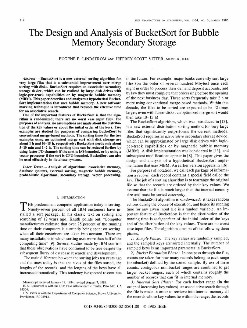
A random sample of S M/K keys is taken, using one ofthe sampling methods discussed in [10] and [18]. The size ofthe sample is an important parameter that is discussed in thenext section. The sample is sorted internally using a balancedsearch tree, such as an AVL-tree [1] or an RB-tree [6], so that

the sorting time overlaps with the sampling as much as possi-ble. Each node in the balanced tree requires storage space forthe key, plus two pointers for the sorting. The key value of theleft son is less than or equal to the key value of the parent;similarly, the key value of the right son is greater than the keyvalue of the parent. A balanced tree for the case ofS = 16 sampled keys is pictured in Fig. 1.The magnetic bubble memory (MBM) is made up of basic

units called arrays, as discussed in Section VI. In the case ofsequential files that must pass through the CPU in order to getstored on the associative MBM, each record is stored in arandom array in the MBM. The sampling is done while therecords are being distributed on the MBM. We can force astable sort by appending a sequence number to the end of thekey field. The actual key field might be scattered in partsthroughout the record, each part in a different data format.For purposes of speeding up the sort, it may be desirable toconvert e4ch key field to binary notation and to reformat therecord so that the binary key value appears at the front of therecord.

If the records of the input file already reside in the MBM,then we assume that they were placed on random arrays. Ifnot, the records should be randomly shuffled among the ar-rays so that the marking technique described in Section VIIcan be used most effectively. The sampling can be donedirectly from the bubble memory at the expense of more logiccomplexity. First, a random variable specifying the numberof keys to be picked from each array of the MBM is gener-ated, based on the multinominal distribution. Then we useone of the sampling methods in [ 10] or [18] in order to samplefrom each array in parallel.The last part of this phase consists of an in-order traversal

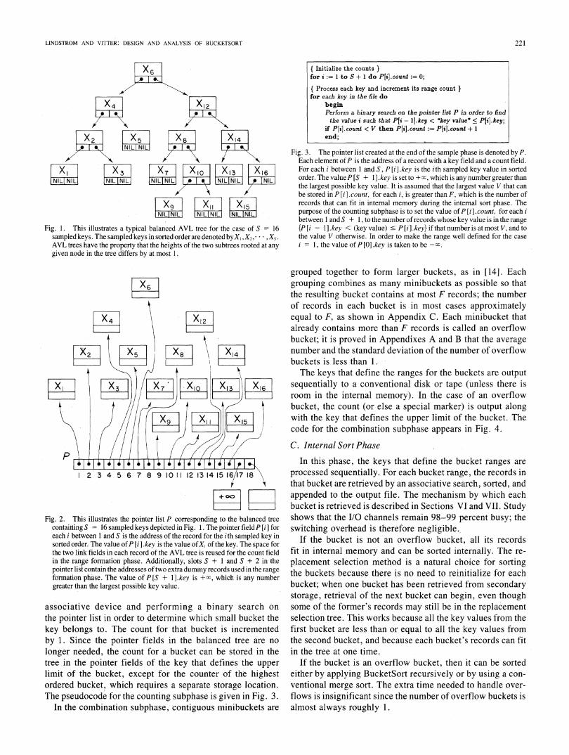
of the balanced tree in order to create a sequential list ofpointers that point to the keys in the tree in increasing order.Fig. 2 depicts the pointer list obtained from the balanced treein Fig. 1.

B. Bucket Formation Phase

This phase is divided into two parts: the counting subphaseand the combination subphase. The S sampled key values thatwere sorted in the Sample Phase break up the file into S + 1minibuckets. Let us denote the sorted key values by

XI,X2, * ,Xs-We also define X0 =- -oc and Xs,I = +oc. For each value ofi, 1 . i . S + 1, the ith minibucket is defined to be the setof records whose key value is in the range

Xi-, < (key value) . Xi.

Each minibucket contains an average of about N/S recordswith a standard deviation of about N/S. In the next section,we discuss how to choose S so that N/S is very much smallerthan F, which is the number of records that can fit in internalmemory.The sorted order of the keys is represented by the se-

quential pointer list that was created at the end of the SamplePhase. The keys are still stored in the balanced tree. Thecounting subphase consists of processing each key on the

220.


X6

X4 X122 X4 l Xl 14

~~IL ~ ~ ~ WL NINIlX2 1 ~1X xioX8X116

NI7 77INIL] [| N

Xg IXii 15INIL| NIL INIL NIL NIL [NIL

Fig. 1. This illustrates a typical balanced AVL tree for the case of S 16sampled keys. The sampled keys in sorted order are denoted byX,, X2, ** , Xs.AVL trees have the property that the heights of the two subtrees rooted at anygiven node in the tree differs by at most 1.

2 3 4 5 6 7 8 9 10 11 12 13 14 15 16178 \

Fig. 2. This illustrates the pointer list P corresponding to the balanced treecontaitningS = 16 sampled keys depicted in Fig. 1. The pointer fieldP [i] foreach i between 1 and S is the address of the record for the ith sampled key insorted order. The value ofP [i].key is the value ofXi of the key. The space forthe two link fields in each record of the AVL tree is reused for the count fieldin the range formation phase. Additionally, slots S + 1 and S + 2 in thepointer list contain the addresses oftwo extradummy records used in the rangeformation phase. The value of P [S + l].key is +oo, which is any numbergreater than the largest possible key value.

associative device and performing a binary search on

the pointer list in order to determine which small bucket thekey belongs to. The count for that bucket is incrementedby 1. Since the pointer fields in the balanced tree are no

longer needed, the count for a bucket can be stored in thetree in the pointer fields of the key that defines the upperlimit of the bucket, except for the counter of the highestordered bucket, which requires a separate storage location.The pseudocode for the counting subphase is given in Fig. 3.

In the combination subphase, contiguous minibuckets are

Fig. 3. The pointer list created at the end of the sample phase is denoted by P.Each element ofP is the address of a record with a key field and a count field.For each i between and S, P [i].key is the ith sampled key value in sortedorder. The valueP [S + l].key is set to +oc, which is any number greater thanthe largest possible key value. It is assumed that the largest value V that can

be stored in P [i] .count, for each i, is greater than F, which is the number ofrecords that can fit in internal memory during the internal sort phase. Thepurpose of the counting subphase is to set the value of P [i].count, for each ibetween and S + 1, to the number of records whose key value is in the range{P [i - 1].key < (key value) ' P [i].key} if that number is at most V, and tothe value V otherwise. In order to make the range well defined for the case

i = 1, the value of P [O].key is taken to be -xc.

grouped together to form larger buckets, as in [14]. Eachgrouping combines as many minibuckets as possible so thatthe resulting bucket contains at most F records; the numberof records in each bucket is in most cases approximatelyequal to F, as shown in Appendix C. Each minibucket thatalready contains more than F records is called an overflowbucket; it is proved in Appendixes A and B that the average

number and the standard deviation of the number of overflowbuckets is less than 1.The keys that define the ranges for the buckets are output

sequentially to a conventional disk or tape (unless there isroom in the internal memory). In the case-of an overflowbucket, the count (or else a special marker) is output alongwith the key that defines the upper limit of the bucket. Thecode for the combination subphase appears in Fig. 4.

C. Internal Sort Phase

In this phase, the keys that define the bucket ranges are

processed sequentially. For each bucket range, the records inthat bucket are retrieved by an associative search, sorted, andappended to the output file. The mechanism by which eachbucket is retrieved is described in Sections VI and VII. Studyshows that the I/O channels remain 98-99 percent busy; theswitching overhead is therefore negligible.'

If the bucket is not an overflow bucket, all its recordsfit in internal memory and can be sorted internally. The re-

placement selection method is a natural choice for sortingthe buckets because there is no need to reinitialize for eachbucket; when one bucket has been retrieved from secondarystorage, retrieval of the next bucket can begin, even thoughsome of the former's records may still be in the replacementselection tree. This works because all the key values from thefirst bucket are less than or equal to all the key values fromthe second bucket, and because each bucket's records can fitin the tree at one time.

If the bucket is an overflow bucket, then it can be sortedeither by applying BucketSort recursively or by using a con-

ventional merge sort. The extra time needed to handle over-

flows is insignificant since the number of overflow buckets isalmost always roughly 1.

{ Initialize the counts }for i := 1 to S + 1 do PIi].count: 0;

{ Process each key and increment its range count }for each key in the file do

beginPerform a binary search on the pointer list P in order to findthe value i such that Pti - 1J.key < "key value" < P[ib.key;

if P[i].count < V then P[i].count := P[iJ.count + 1end;

221


{ Initialize }Output key value -oo;i := 1;P[S + 21.count := F + 1;

while i < S + 1 dobegin { Form next combined range }sum := Pli].count;if sum > F then { Process overflow range

Output a special marker, sum, and P[il.keyelse begin { Process non-overflow range

while sum + P[i + 1J.count < F dobeginsum *= sum + P[i + 1J.count;t :=+ 1end;

Output P[il.keyend;

i:= i 1end;

Fig. 4. The values P [i].key, for each i between 1 and S, are the sampled keyvalues in sorted order. The value ofP [S + l]. key is set to + 7c, which is anynumber greater than the largest possible key value. The largest number that canbe stored in P [i ] .count, for each i, is denoted by V. The value of V is greaterthan F, which is the number of records that can fit in internal memory duringthe internal sort phase. The valueP [i ]. count, for each i between 1 and S + 1,is the maximum of V and the number of records whose key value is in the range{P[i - l].key < (key value c P[i].key}. In order to make the range welldefined for the case i = 1, the value of P [0].key is taken to be -xc. Forprogramming simplicity, it is assumed that there is an extra count fieldP [S + 2]. count. The output of the tombination subphase is the list of keyvalues that define the endpoints of the combined ranges.

IV. CHOICE OF SAMPLE SIZE S AND INTERNAL MEMORYSIZE M

One of the key ideas in BucketSort is the way in which thenumber S of sampled keys and the required amount M ofinternal memory are determined. The sample size S is chosenso as to minimize M subject to the constraint that the averagenumber and the standard deviation of the number of overflowbuckets should be less than 1. (In reality, the resulting valueof M is not the minimum possible, but very nearly so.)

All the formulas in this section are derived in Appendix A.The values of M and S are related by the formula

M - 2BK--+ B (4-1)K + 3P

where B is the size of the input buffer. The values ofM andS can be computed by solving two equations in two unknownsM and r where r is defined to be F(S + l)/(N + 1). The firstequation, which appears as (A-7) in Appendix A, guaranteesthat the above objective will be satisfied

r I r--jn(N +1) (R ±P)\(-2Iln r = ln(&M - 2(B + B ')) (4-2)

where B and B' are the sizes of the small input and largeoutput buffers, respectively, and P is the number of bytes perpointer field. The second equation

(M - 2B + K + 3P)(M - 2(B + B'))= r(N + 1)(R + P)(K + 3P) (4-3)

which appears as (A-8) in Appendix A, specifies that the Ssampled keys can be sorted internally. The value of M ob-tained by solving these two equations is given in Section VIII

for two large-scale sorting examples. It is approximatelyequal to

M- <(ln(N) + 1nQln(NR;K)) NRK + 2B' (4-4)

V. MODIFICATIONS OF BUCKETSORT

When the records are variable-length rather than fixed-length, BucketSort can be modified as follows. We redefineR to be the average record length. Instead of counting thenumber of records in each minibucket during the BucketFormation Phase, we instead count their total lengths. Mini-buckets can be combined into larger buckets as long as thetotal size of all the records is less than the available internalmemory space. The sizes of the I/O buffers should be in-creased to the size of the largest record, Sorting performanceshould still be very good.

BucketSort can also handle the case where several recordshave the same key value. All the records with a given keyvalue will belong to the same minibucket since the binarysearch in the Bucket Formation Phase will end at the sameminibucket in each case. If Xi-I1 Xi, for some 1 ' i .S + 1, all the records in the ith minibucket have the same keyvalue and do not have to be sorted, regardless of the size ofthe bucket. In the case of an overflow bucket for whichX'_ * Xi and there are several identical keys, one repartitionof the bucket should be sufficient to obtain buckets that canbe sorted internally or that consist of only one key value.

There are several places where the running time andmemory required by BucketSort can be reduced. The firstmodification involves the use of the independent and uniformdistribution assumption when appropriate. A small portion ofinternal memory in the Internal Sort Phase is devoted to thefollowing secondary process. The range of 256K possible keyvalues is uniformly divided into approximately cNR/M equalsized intervals, for some constant c > 1. As each key isprocessed, the counter for the [(cNR/M) (key value)/256K]thinterval is incremented where [x] denotes the largest integer.x. If the independent and uniform distribution of key valuesis a valid assumption, that is, if the first few bytes of each keypartition the keys well, then the pass through the file in theBucket Formation Phase can be skipped, and the counts ofthe uniform intervals can be used instead. This modifi-cation takes advantage of the fast partitioning when the keysare evenly distributed, while still maintaining the originalrandom sampling approach in case the keys are not evenlydistributed.

The second modification reduces the amount of internalmemory required by BucketSort, which is calculated in Sec-tion VIII for two extremely large sorts, at the expense ofhaving to sort the S sampled keys in the Sample Phase exter-nally. If the internal memory M is reduced by a factor of c,for some c > 1, then the number of buckets is increased byroughly that factor, so at least c times as many keys as beforewill have to be sampled. For exampple, if we reduceM by half,the sampled keys will fill up the internal memory slightly

222


more than four times. The counting subphase will have tobe done one memory load at a time, but if the bottleneckin the counting subphase is the channel speed (which israther likely), there will be little increase in elapsed time forthat subphase.The third modification deals with speeding up the counting

subphase in- the Bucket Formation Phase. If a pipelined CPUis available, the N keys from the associative disk can beprocessed in 0 (N) time rather than 0 (N log, S) time, whichis a significant improvement if the counting subphase isa bottleneck.The fourth modification is to resample and repartition the

overflow buckets during the Bucket Formation Phase ratherthan during the Internal Sort Phase, at the cost of some extrainternal storage space. This allows the Internal Sort Phase toproceed smoothly without interruption and with only a singleinitialization of the replacement selection tree.The final modification speeds up the Internal Sort Phase if

it is CPU-bounded. The internal memory is approximatelydoubled and partitioned into two halves. The records from thecurrent bucket can be sorted in one half, while in the otherhalf, the sorted records from the previous bucket are outputto the disk and the unsorted records from the next bucket are

retrieved from the disk. Since each internal sort is now staticrather than dynamic in nature, we can use quicksort or radixsort rather than the slower replacement selection. In addition,quicksort and radix sort can take advantage of vector featuresof the CPU. Preliminary studies indicate that quicksort andradix sort can be more than twice as fast with vector process-

ing than without, provided that certain vector features are

available [16]. This is discussed further in Section X.

VI. THE USE OF BUBBLE MEMORY AS AN AsSOCIATIVESECONDARY STORE

The basic requirement for the associative secondary stor-age device is that it must be able to process the followingassociative search (or range query) in about 1 or 2 s:

Given values a and b,retrieve all records in the range

{a < (key value) b}. (6-1)Let us denote the time per associative search by T. This typeof search is performed once for each bucket range during theInternal Sort Phase of BucketSort, and accounts for the greatmajority of the execution time. In this section, we study howto implement the associative secondary storage by use ofmagnetic bubble memory (MBM). The use of bubble mem-

ory for associative secondary storage in dat-abase applicationsis discussed in [3]-[5].

In this paper, we shall refer to the following structuralorganization of the MBM, which is based on a proposedproduct in industry. The top-level unit of the MBM is calleda box, which consists of roughly 256 megabytes. For engi-neering reasons, boxes are composed of several levels ofhierarchy. Each box consists of four independent units calledboards. A board consists of 16 modules, which are divided

into smaller units called chips, which in turn contain severalbasic units called arrays. For our purposes, we can considereach box as consisting of 2000 arrays.

Each array contains one Mbit of storage, as pictured inFig. 5. There are 1000 synchronous minor loops, each con-taining 1000 bits (magnetic bubbles) rotating around the loopin response to a changing magnetic field. Records are stored"horizontally across" the minor loops: the kth bit of the ithrecord in the array is stored in the ith bit of the kth minorloop. Records containing more than 1000 bits must be sub-divided into 1000-bit pieces. The pieces can be stored in oneof two ways (or a combination thereof): 1) the pieces can bedistributed among several arrays, one piece per array; or2) the pieces can be stored on contiguous rows across theminor loops of one array.

For reasons of efficiency, we shall assume that the firstalternative is used to store the records. All the bits of a givenrecord arrive at the top of the minor loops at the same time.We assume that the reading mechanism is nondestructive.A read is accomplished by duplicating each bit and loadingthe duplicate bits into the 1000 loop read buffers. When theread shift register (RSR) is empty and available, the bitsare loaded into the RSR. The bits in the RSR are thenshifted sequentially to the read buffer. Writes are accom-plished in a similar way using the write shift register (WSR)and the write buffer.At the module level in the hierarchy, there is a micro-

processor and some random access memory (RAM) thatserves as a read/write buffer. An associative search consistsof transferring each record from the array via the RSR to theread/write buffer. The microprocessor selects and keeps inthe buffer all the records whose key values satisfy the rangequery (6-1). Depending on the nature of the retrieval, eachselected record or perhaps only parts of it are transferred fromthe buffer to the CPU.The period of time required for the circulation of the minor

loops in an array is equal to the time it takes to move the1000 bits in the RSR to the read buffer, which is 0.001 s.When the shift is completed in the RSR, the 1000 loop readbuffers have had time to load the next record. Hence, theentire contents of an array can be loaded into an RSR and readin 1000 x 0.001 = 1 s. All the arrays in all the boxes aresearched in parallel, which means that the total time for anassociative search is 1 s.

There are an average of two 1000-bit buffers per array. Thebuffers are located at the module level of the MBM hierarchy,so that several arrays can share a pool of buffers. (Theamount of buffer space required can be decreased somewhatwithout degradation in BucketSort performance; however,this amount of buffer space is not unusual since it is prefer-able for other possible uses of the MBM in non-BucketSortapplications, such as a fast cache for a magnetic disk or as amagnetic disk replacement.)The associative search mechanism can be better under-

stood by considering a bucket retrieval in the Internal SortPhase. Each record is tested for membership in the currentbucket by a microprocessor while the record is stored in theRAM read/write buffer. When a record belongs to the bucket

223


Array(O16 bits)

read shift register (RSR)l

loopes bfe

error code

ffi write shift register (WSR) l

Fig. 5. The basic structural unit of MBM is the array, enclosed by the dashed lines. The 1 Mbit array consists of 1000 minorloops, each ioop containing 1000 rotating bits (magnetic bubbles).

currently being retrieved, it is kept in the buffer until it istransferred over the channel to the CPU. If all the buffers ina module get full, then any array in the module that needs anew buffer to continue searching must halt its RSR tempo-rarily until buffer space becomes available. This delays theassociative probe for that array.Each board in the MBM has an associated controller that

provides access to the I/O channel (or bus). During bucketretrieval, each controller maintains a queue consisting of themicroprocessors (at the module level) that have records readyto be transferred to the CPU. The channel selectively choosesa controller and transfers to the CPU all the records of thefirstmicroprocessor on the queue. For maximum efficiency, thecontroller is chosen using a round-robin daisy chain scheme(see [2], for example). We denote the overhead time requiredfor the daisy chain to select a subsequent controller by ohdaiSy.Typically, the next controller can be selected while the cur-rent controller is broadcasting its records to the CPU. Eachtime the channel chooses a new controller (which may be thesame as the current controller), a certain switching overheadtime ohI is incurred by the channel in order to update theorigination and destination addresses for the I/O. There is asmaller switching overhead time oh2 between consecutiverecords broadcast by the same controller. Conservative esti-mates for these switching overheads are ohdaisy 10 ,us,oh, = 10 .ts, and oh2 1 ,us. Simulations of the bucket re-trieval process are described in Section IX.The number of records that are transferred from MBM to

internal memory during a bucket retrieval is roughly MIR,which can be extremely small compared to N. In the ex-amples we discuss in Sections VIII and IX, the average num-ber of records from a given array that belong to the currentbucket being retrieved is less than 1! In such cases, the delay

caused by buffers becoming full is insignificant. Extensivesimulations by the authors have shown that the resultingbucket retrieval time for the two sorting examples in Sec-tion VIII are 1.001 T and 1.04 T, which represents a neg-ligible increase over the ideal retrieval time of T. Thesesimulations take into account both the delays caused by fullbuffers as well as the switching overheads described in thelast paragraph.The marking technique introduced in the next section re-

duces the search time so that the channel speed becomes thebottleneck. Simulations reveal that when the marking tech-nique is used during large sorts, the channels remain98-99 percent busy. This important fact is discussed furtherin Section IX.

VII. SPEEDING UP THE BUCKET RETRIEVALS

In the Internal Sort Phase, an associative search as in (6-1)is performed to retrieve each bucket. The search done in thenaive way described'above requires about 1-2 s. The channelthat connects the MBM to the CPU may be able to transferMbytes (one internal memory load) in only a fraction of asecond'. In that case, the bottleneck is the search time. Thissection is devoted to software marking techniques that re-move this bottleneck by speeding up the time per bucketretrieval, so that the rate of a bucket retrieval matches thechannel speed.Roughly one out of every NR/M records in the file belongs

to a given-bucket, so almost all the bucket retrieval time in-volves processing records that do not satisfy the range query(6-1). The key to speeding up the bucket retrievals is toavoid having to process most of these records. To accomplish

224


that, we need one extra bit per record, which we store in theMBM and use as a mark bit. Records may be either markedor unmarked. The MBM architecture must be modified tosupport a special reading mode in which only marked recordsare transferredfrom the minor loops to. the RSR. Each rangequery now has the form:

Given values a and b,retrieve all marked records in the range{a < (key value) < b}. (7-1)

The following simple example illustrates how we can re-duce the time per bucket retrieval by a factor of k, for any1 ' k << NR/M. A detailed analysis is given at the end ofthe section. We assume that during the combination subphaseof the Bucket Formation Phase, we have stored the k - 1ordered key values that partition the buckets into k roughlyequal-sized groups. We shall denote the k - 1 ordered keysplus the dummy keys -cc and +oo by

-o = YO, Y1, Y2, , Yk-1, Yk =+0

The Internal Sort Phase can be divided into k sequentialsubphases. The ith subphase involves the retrieval and sort-ing of all the buckets in the range between YFi and Yi. Thenew twist is that we do the following preprocessing at thebeginning of the ith subphase, for i = 1, 2, ,k:

Mark all the records in the range{Yi l < (key value) . Yi}and unmark the others. (7-2)

Roughly N/k records are marked at any one time, so thenumber of processed records in each bucket retrievaldecreases by a factor of k. Each of the k preprocessing steps(7-1) requires one complete associative search (which is1-2 s), but as long as k is not too large, the total pre-processing time is negligible.We can do even better if during each bucket retrieval we

turn off the mark bits of all the records that satisfy the rangequery. At the beginning of each subphase, roughly N/krecords are marked, but the number of marked records de-creases linearly until it becomes 0 at the end of the subphase,as pictured in Fig. 6. The average number of records that areprocessed for each bucket retrieval is now approximatelyN/(2k).

In addition, the range query (7-1) can be replaced by thefollowing query that involves only one comparison ratherthan two:

Given value bretrieve and unmark all marked records such that(key value) ' b. (7-3)

This query is equivalent to (7-1) because by the time thebucket range {a < (key value) ' b} is processed, all therecords with (key value) - a have already been unmarked.An alternate way to reduce the time per bucket retrieval

without using mark bits is to distribute the records in range[Yi1I, Yi] evenly among all the arrays, in predetermined lo-cations on each array. Thus, when a bucket in range [Y1l, Yi ]must be retrieved, only the records known to be in the rangemust be processed, thus reducing the processing time to a

- Nw

Lu

H

Luy0

m N/kILi0-

0LucoUn

0

(I)0

o 0o -O:U

41',

II= YO Y,

MEDIAN

Y2 Y3VL .yTH Yk =+E

KEY VALUE IN THE BUCKET

Fig. 6. This illustrates the effectiveness of the marking technique. The num-ber of records processed during a bucket retrieval is graphed as a functionof which bucket is being retrieved.

fraction of a second. (A similar idea was developed in [8] forimproving the bucket retrieval time in the logic-per-trackdisk implementation of BucketSort in [13]. In the disk imple-mentation, the records in the range [Yi71, YiI, which is calleda maxibucket, are distributed on a minimum number of adja-cent cylinders. However, an extra pass of the input filethrough the CPU is required because the distribution of therecords onto adjacent cylinders cannot begin until the count-ing subphase has been completed. This tends to offset some-what the improvement in running time in the disk version.)

A. Modifications of the Marking Technique

Each preprocessing step (7-2) can also be done with onlyone comparison in a naive way that requires two passes overthe file. It can be done in only one pass if two mark bits Mland M2 are used for each record: Ml for the preprocessing andM2 for the unmarking when a record satisfies the range queryduring a bucket retrieval. Initially, all the records areMl-unmarked and M2-marked. Each preprocessing step (7-2)is replaced by

MI-mark all M2-marked records such that(key value) < Yi (7-4)

The time per step decreases linearly from T (for i = 1) to Tlk(for i = k). Range query (7-3) is replaced byGiven value b, retrieve and Ml-unmark and M2-unmarkall MI-marked and M2-marked records such that(key value) ' b. (7-5)If multicomparison range queries are allowed, then the

preprocessing (7-2) can be done during the retrieval of thefirst bucket in the ith subphase. If significantly more RAM isavailable, then several buckets can be processed at once, asfollows. The records in the first range are transferred tothe CPU internal memory as usual, and the addresses ofthe records in each of the remaining buckets are stored in the

225


RAM. Retrieval of those buckets is done one at a time in arandom access mode using the lists of addresses that residein the RAM. Since the individual arrays can be accessed inparallel, each transmitting a record in 0.001 s, the recordsin a bucket can be accessed orders of magnitude faster thisway than by an associative search. The channel speed to theCPU would definitely be the bottleneck in this case. Analternative to storing the lists of addresses is to use extra markbits per record, but that requires even more RAM space.A modification suggested by K. Belser is to retrieve each

bucket by parallel random access rather than by an associa-tive search. A list of the addresses of the records in eachminibucket must be stored in the RAM during the countingsubphase of the Bucket Formation Phase; this can be over-lapped with the counting. This requires enough RAM to storean address for each of the N records in the MBM. Eachaddress might require about 3 bytes, so the total amount ofRAM in the bubble unit could be rather excessive. As in thelast paragraph, the time to select the records in each bucketwould be very fast, so time per bucket retrieval would still belimited by the channel speed to the CPU internal memory.The marking technique discussed earlier in this section ispreferable in most cases since it requires much less RAM andcan still match the rate of a bucket retrieval to the channelspeed.

B. Analysis of the Marking Technique

The rest of this section is devoted to a more realistic assess-ment of the marking technique. If we do the preprocessing asin (6-1) and (6-2) using k subphases, the time to access therecords in a bucket will be reduced by some factor less thank, for the reasons given below. The net effect is that thenumber k of subphases should be increased slightly to havethe desired effect.The first complication deals with the fact that the arrays are

searched in parallel during a bucket retrieval, and that somearrays take longer to search (i.e., they contain more markedrecords) than others. The total search time is equal to themaximum search time among all the arrays. The search timeis related to the number of marked records in the array thatcontains the most marked records. Let us denote that value byAmax. We can get a good approximation of Amax by model-ing the number of marked records in each array as an inde-pendent normal random variable with mean ,u and standarddeviation v. If we denote the number of subphases byk, then the average number of marked records in eacharray is ,u - 1000/k, and the standard deviation is Co=

100O(k - 1)/k2. By the theory of statistics of extremevalues [7], we have Amax -, + to, where the first-orderapproximation to f is A2 ln(0.4N/ 1000). Experiments con-firm that this approximation for Amax is correct to within2 percent for large sorts, like those considered in the nextsection. For the case N i07, k = 5, the average value ofAmax is roughly 250, whereas the average number of markedrecords in each array is 200. Hence, the search time for thefirst bucket in each subrange is reduced by a factor of1000/250 = 4 rather than by a factor of 1000/200 = 5. The

search times for the remaining buckets in the subphase de-crease as more and more records get unmarked.

Another complication occurs when the physical records ofthe MBM are larger than the logical records in the file. Thephysical record size in the MBM is determined by the num-ber of arrays that are packed together into one independentunit. For example, if 32 arrays are driven by the samemagnetic field, then for all practical purposes we have one"super array," which is called a module, consisting of32 x 1000 synchronized minor loops, each containing1000 bits. The physical record size is 32 Kbits, which is4 Kbytes.

Let us use b ' 1 to denote the ratio of the physical recordsize to the logical record size. If the logical record size in aBucketSort application is 1 Kbyte in the above example, thenb = 4 logical records must be packed into each physicalrecord. The mark bits are associated with the physicalrecords, not the logical records; there is one mark bit for eachphysical record. The physical record is marked when any ofthe logical records it contains should be "marked." If we usefour subphases with the marking technique, then each sub-phase may have all the physical records marked since eachphysical record might contain one logical record in eachof the four quadrants! The choice a larger number k = k 'b ofsubphases will guarantee that there will be at most N/k'marked records. The choice k = -b/ln(I - I/k') sub-phases will produce an average of N/k' marked physicalrecords.

VIII. Two EXTREMELY LARGE SORTING EXAMPLES

The following two examples represent extremely largesorting applications. The first example illustrates the sizes ofthe sorts done once a night by major banks; the second ex-ample is the projected size of large sorts within this decade.

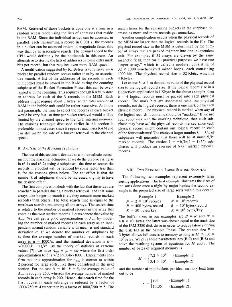
Example 1 Example 2N = 2 X 106 records N = 107 recordsR = 400 bytes/record R = 103 bytes/recordK = 50 bytes/key K = 102 bytes/key

The buffer sizes in our examples are B = R and B' =4.8 x 104 bytes; the latter was chosen equal to the track sizeof the IBM 3380 disk drive in order to reduce latency duringthe disk I/O in the Sample Phase. The pointer size P =3 bytes allows full access to memory as long as M ' 1.6 x107 bytes. We plug these parameters into (B-7) and (B-8) andsolve the resulting system of equations for M and r. Thenumber of bytes of required memory is

t7.2 x 105 (Example 1)13.4 x 106 (Example 2)

and the number of minibuckets per ideal memory load turns

out to be

r9.4r =

10.35

(Example 1)(Example 2).

226

LINDSTROM AND VITTER: DESIGN AND ANALYSIS OF BUCKETSORT 227

As pointed out in Section III, M is roughly equal to

l(ln()NR + In ln(NR/K)))NRK + 2B'

and S is equal to (M - 2B)/(K + 3P).The memory requirement for Example 2 is large, but not

excessive, considering that large sorts like Example 2 will bedone only by companies with extensive computer facilities.One of the modifications in Section IV allows the memoryrequirement M to be reduced at the expense of having to sortthe S keys in the sample phase externally, which takes littleextra time compared to the total sort time. We can also de-crease M by roughly 100 Kbytes if we use faster channels toconnect the CPU to the MBM since we could then use smalleroutput buffers in the Internal Sort Phase, as discussed inAppendix A.

IX. SORTING TIME FOR THE EXAMPLES

In this section, we estimate the running time of BucketSortfor the two examples in Section VIII, based upon the formu-las derived in Appendix D. The associative secondary storeconsists of the magnetic bubble memory described inSections VI and VII. The time T per associative search isassumed to be 1-2 s, as explained in Section VI. The chan-nel rate is assumed to be C = 3 x 106 bytes per second,which is extremely conservative for MBM since MBM canutilize a much higher channel rate (perhaps by using fasterchannels, several channels, or a memory bus attachment).

Before we analyze the running times of the three phases ofBucketSort, it is important to determine the channel utiliza-tion. The channel utilization is the percentage of time inwhich the channel is transferring useful information. Theutilization is decreased by switching overhead time and byperiods in which no controller is ready to transmit.

Let us consider the channel utilization in the Internal SortPhase. As we shall see later in this section, the InternatSortPhase accounts for the predominant portion of the runningtime of BucketSort. It consists of consecutively retrieving therecords in each bucket from MBM and then sorting theminternally. We shall see soon that the internal sorting time cantypically be overlapped with the retrieval. The use of themarking technique described in Section VII is designed toreduce the time required for an associative probe so that theretrieval time is dominated by the channel speed. An obviouslower bound on the retrieval of a single buck&t is therefore

R x number of records in the bucketC . -~~~~(9-1)

The actual retrieval time is slightly longer for the followingreasons.

1) If the buffers on the MBM get full, some of the RSR'smight be temporarily stopped until buffer space becomesavailable, as described in Section VI.

2) There are overheads ohdaisy, oh1, and oh2 incurred when

the origination and destination addresses for the I/O are up-dated, as described in Section VI.

Extensive simulations carried out by the authors show that,for the two examples in the last section, the channel utiliza-tion is 98-99 percent. In other words, the channels remainalmost totally busy. Formula (9-1) thus gives a valid accountof the bucket retrieval time.

Several other interesting facts have been uncovered by thesimulations. For example, it is possible to reduce the amountof buffer space by a factor of four with only a small effecton the bucket retrieval times. The simulations also verifiedthe approximations for A,max, the average number of markedrecords in the array that contains the most marked records,given near the end of Section VII. We have Amax +tcr, where , = 1000/k, r = \/1000(k - 1)/k2, and tiA2 ln(0.4N/1000). In order to reduce the time for an asso-ciative probe so that the channel remains busy, it suffices tochoose a number of subphases k so that Amax x 0.001 <0.9M/C. For the two examples in Section VIII, the choicesk = 6 (ENample 1) and k = 1 (Example 2) are sufficient.Some of the results of the simulations are given in Tables Iand II. The channel utilization is plotted as a function of thenumber k of subphases and of the average number of buffersper array.

In the rest of this section, we apply the analysis givenin Appendix D of the running time of the three phases ofBucketSort to the two examples in the last section.

A. Sample PhaseIf the input file is already stored on the MBM, then (D- 1)

gives the time for the Sample Phase. The process is probablyI/O bounded, so the total time is at most SK/C + c2 SK,which is bounded by 1-2 s.

If the input file does not reside on the MBM, then by (D-2)the time for the Sample Phase will be about NR/C + C2 SK s.

Plugging in the values of the parameters, we obtain the timebounds of roughly 5 min (Example 1) and 58 min (Ex-ample 2).


Both quantities in the first part of (D-3), the formula for thecounting subphase, are on the order of /2 min (Example 1)and 6 min (Example 2). The time for the combination sub-phase, which is the second part of (D-3), is approximately(r/(r - 1))NK/FC s, which is a fraction of 1 s for both ex-

amples. Here F - M/R is the number of records that can fitin internal memory; a formula for F is derived in Ap-pendix A.

C. Internal Sort PhaseFor both examples, the preprocessing time kT for the mark-

ing technique is insignificant. We can expect that the timerequired to sort each bucket, which is given by (D-4) for theunmodified algorithm, is bounded by the I/O time FR/C. Weshow in Appendix C that the number of iterations is equal toapproximately (r/(r - 1))N/F + 2. The average total timerequired for the Internal Sort Phase is therefore bounded by

IEEE TRANSACTIONS ON COMPUTERS, VOL; c-34, NO. 3, MARCH 1985

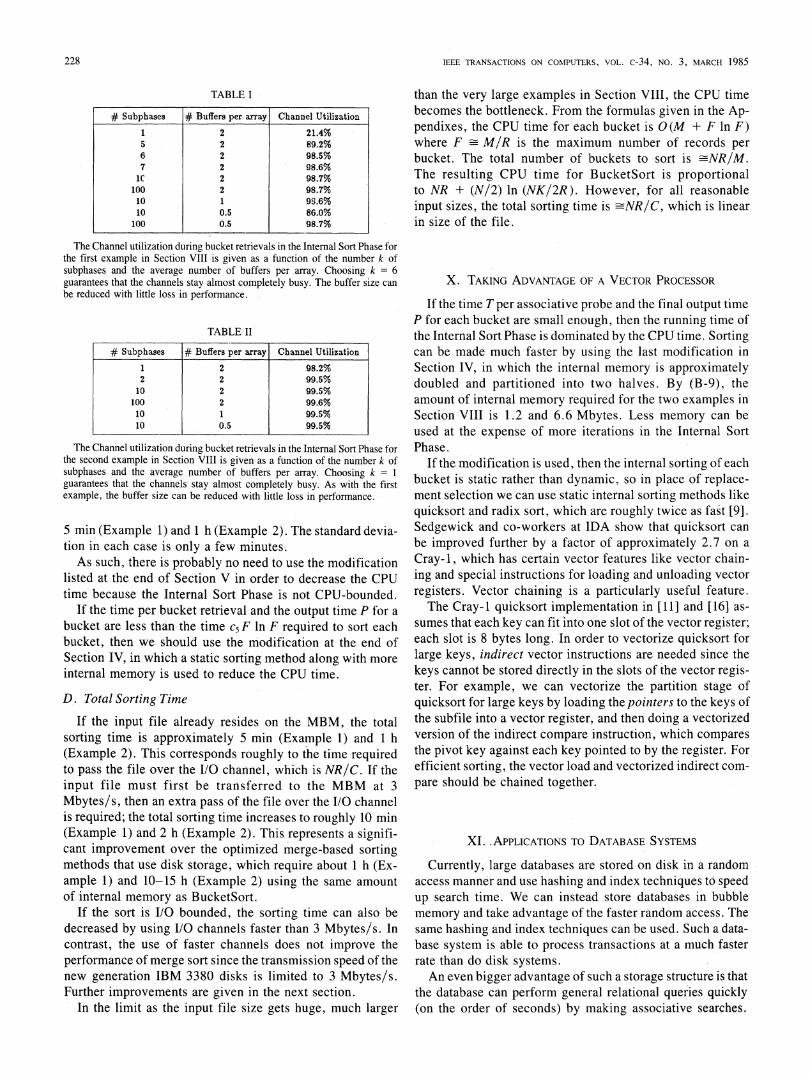
TABLE I

# Subphases # Buffers per array Channel Utilization

1 2 21.4%5 2 89.2%6 2 98.5%7 2 98.6%

iC 2 98.7%100 2 98.7%10 1 98.6%10 0.5 86.0%

100 0.5 98.7%

The Channel utilization during bucket retrievals in the Internal Sort Phase forthe first example in Section VIII is given as a function of the number k ofsubphases and the average number of buffers per array. Choosing k = 6guarantees that the channels stay almost completely busy. The buffer size canbe reduced with little loss in performance.

TABLE II

# Subphases # Buffers per array Channel Utilization1 2 98.2%2 2 99.5%

10 2 99.5%100 2 99.6%10 1 99.5%10 0.5 99.5%

The Channel utilization during bucket retrievals in the Internal Sort Phase forthe second example in Section VIII is given as a function of the number k ofsubphases and the average number of buffers per array. Choosing k = 1guarantees that the channels- stay almost completely busy. As with the firstexample, the buffer size can be reduced with little loss in performance.

5 min (Example 1) and 1 h (Example 2). The standard devia-tion in each case is only a few minutes.As such, there is probably no need to use the modification

listed at the end of Section V in order to decrease the CPUtime because the Internal Sort Phase is not CPU-bounded.

If the time per bucket retrieval and the output time P for abucket are less than the time c5 F ln F required to sort eachbucket, then we should use the modification at the end ofSection IV, in which a static sorting method along with moreinternal memory is used to reduce the CPU time.

D. Total Sorting Time

If the input file already resides on the MBM, the totalsorting time is approximately 5 min (Example 1) and 1 h(Example 2). This corresponds roughly to the time requiredto pass the file over the I/O channel, which is NR/C. If theinput file must first be transferred to the MBM at 3Mbytes/s, then an extra pass of the file over the I/O channelis required; the total sorting time increases to roughly 10 min(Example 1) and 2 h (Example 2). This represents a signifi-cant improvement over the optimized merge-based sortingmethods that use disk storage, which require about 1 h (Ex-ample 1) and 10-15 h (Example 2) using the same amountof internal memory as BucketSort.

If the sort is I/O bounded, the sorting time can also bedecreased by using I/O channels faster than 3 Mbytes/s. Incontrast, the use of faster channels does not improve theperformance of merge sort since the transmission speed of thenew generation IBM 3380 disks is limited to 3 Mbytes/s.Further improvements are given in the next section.

In the limit as the input file size gets huge, much larger

than the very large examples in Section VIII, the CPU timebecomes the bottleneck. From the formulas given in the Ap-pendixes, the CPU time for each bucket is 0 (M + F ln F)where F -M/R is the maximum number of records perbucket. The total number of buckets to sort is -NR/IM.The resulting CPU time for BucketSort is proportionalto NR + (N/2) ln (NK/2R). However, for all reasonableinput sizes, the total sorting time is -NR/C, which is linearin size of the file.

X. TAKING ADVANTAGE OF A VECTOR PROCESSOR

If the time T per associative probe and the final output timeP for each bucket are small enough, then the running time ofthe Internal Sort Phase is dominated by the CPU time. Sortingcan be made much faster by using the last modification inSection IV, in which the internal memory is approximatelydoubled and partitioned into two halves. By (B-9), theamount of internal memory required for the two examples inSection VIII is 1.2 and 6.6 Mbytes. Less memory can beused at the expense of more iterations in the Internal SortPhase.

If the modification is used, then the internal sorting of eachbucket is static rather than dynamic, so in place of replace-ment selection we can use static internal sorting methods likequicksort and radix sort, which are roughly twice as fast [9].Sedgewick and co-workers at IDA show that quicksort canbe improved further by a factor of approximately 2.7 on aCray-1, which has certain vector features like vector chain-ing and special instructions for loading and unloading vectorregisters. Vector chaining is a particularly useful feature.The Cray-1 quicksort implementation in [11] and [16] as-

sumes that each key can fit into One slot of the vector register;each slot is 8 bytes long. In order to vectorize quicksort forlarge keys, indirect vector instructions are needed since thekeys cannot be stored directly in the slots of the vector regis-ter. For example, we can vectorize the partition stage ofquicksort for large keys by loading the pointers to the keys ofthe subfile into a vector register, and then doing a vectorizedversion of the indirect compare instruction, which comparesthe pivot key against each key pointed to by the register. Forefficient sorting, the vector load and vectorized indirect com-pare should be chained together.

XI-. APPLICATIONS TO DATABASE SYSTEMS

Currently, large databases are stored on disk in a randomaccess manner and use hashing and index techniques to speedup search time. We can instead store databases in bubblememory and take advantage of the faster random access. Thesame hashing and index techniques can be used. Such a data-base system is able to process transactions at a much fasterrate than do disk systems.An even bigger advantage of such a storage structure is that

the database can perform general relational queries quickly(on the order of seconds) by making associative searches.

228


This cannot be done when disk storage is used. In otherwords, the bubble memory can be used either as a randomaccess device or as an associative device, whichever is moreefficient for the current transaction or query. The mark bitsused by BucketSort to speed up the bucket retrieval in theInternal Sort Phase, as described in Section VI, are also veryhelpful for performing relational queries [4], [17]. Bucket-Sort can be viewed as one of the operations of the relationaldatabase system.

XII. CONCLUSIONS

We have shown that BucketSort is an extremely fast sort-ing method for very large files. In our average case analysis,we make no assumptions about the distribution and bias of thekey values or about the initial order of the keys. There are noworst case input files. For the two examples in Section VIII,a conservative analysis shows that BucketSort is faster thanoptimized merge-based methods that use disk storage by afactor of roughly 10.One of the main contributions of BucketSort is the sam-

pling technique used to partition the file into roughly equalsized bucket ranges. This technique should prove useful inother sorting and searching applications in which files mustbe processed one memory load at a time.The internal memory requirements of BucketSort are high,

but reasonable, considering that the very large sorts dis-cussed in this paper will be done only in large computerinstallations. As explained in Section IV, roughly MV(ln(NR/K) + ln(ln(NR/K)/2))NRK/2 + 2B' bytes of in-ternal memory are needed. We have shown that the associa-tive secondary storage device can be realized effectivelyby using magnetic bubble memory (MBM), which canperform an associative search in 1-2 s. The software mark-ing techniques discussed in Section VI can reduce the searchtime for this application to a fraction of a second. The use oflogic-per-track disks for associative storage is discussed in[8] and [13].The Internal Sort Phase dominates the total sorting time.

The resulting sorting time is approximately NR/C for prac-tical file sizes, even for the large examples considered inSections VIII and IX. In Appendix C, we show that the num-ber of iterations (i.e., the number of buckets) is roughlyNR/M. The sorting of each bucket can usually be overlappedwith the I/O time per bucket, which is approximately FR/Cwhere F M/R is the maximum number of records perbucket. For extremely large sorts, the CPU time for eachbucket, which is 0 (M + F log F), will be the, bottleneck.When that is the case, we can cut the CPU time in half at theexpense of roughly double the internal memory space. Inaddition, if the CPU has the required vector features, likechaining and certain vector instructions, then the CPU timecan be reduced further by a factor of 2-3.

BucketSort has other advantages also. If the sort is I/O

used in database systems. In summary, BucketSort is an effi-cient solution to the problem of sorting massive files.

APPENDIX AANALYSIS OF THE REQUIRED AMOUNT OF

INTERNAL MEMORY M

In this section, we calculate the amount M of internalmemory needed to assure that for every input file the averagenumber of overflow buckets will be less than 1. Of course,the average number of overflow buckets can be decreasedfurther if we allocate even more internal memnory to Bucket-Sort. The number of iterations in the Internal Sort Phase, andpossibly the total sort time, will also decrease appropriately.The sorted sample of S keys (with -xc and +oc added

as delimiters)-o = Xo,XI,X2, . XSRXS1 = +00

divides the N records into S + 1 minibuckets. The ith mini-bucket consists of all the records whose key value is inthe range

{Xi-, < (key value) . X'}.

We denote the number of records in the ith minibucket by Ni.For 1 ' i ' S, the probability that the ith minibucket con-tains exactly b records where 1 . b N - S + 1 is

Nb-Nb

Prob{N, = b} = -s I(A-1)

where (') denotes the binomial coefficient n!/(m!(n - m)!).The last minibucket contains one less record on the averagesince Xs+, +x is not part of the actual sample. We have,for 0 ' b N -S,

Prob{Ns,i = b} - (

For convenience in getting an upper bound on the frequencyof overflow, we assume that all S + 1 minibuckets havedistribution (A-1). The average value of Ni is

( N -b N + NS b S - I S + I

(A-2)

We can show easily that the standard deviation is equalto V\(N + 2)(N + 1)S/(S + 2) (S + 1)2, which is slightlyless than the mean. The probability that the ith minibucketcontains more than b records is

bounded, sorting time can be decreased by using faster I/Ochannels. The space and time efficiency can be improved byone of several other mnodifications. BucketSort can also be

tN- N bProb{Ni > b} ( b N-(S) (A-3)

229


where n' denotes the "falling power" n!/(n - m)!=n(n - 1) .. *(n - m + 1).

Our strategy that limits the number of overflow buckets isbased on choosing a large sample size S such that the averageminibucket size (N + l)/(S + 1) will be much less than F,which is the number of records that can fit in internal mem-ory. The value of F is equal to (M - 2(B + B'))/(R + P)where B is the size of the -two input buffers and B' is the sizeof the two output buffers in the Internal Sort Phase, and P isthe size of the pointer required by each record for the replace-ment selection. If the rate of output is steadily faster than thetransmission speed of the output storage device (e.g., if fasterchannels to the MBM are used), then the output buffer size B'can be reduced to B, which will decrease the amount M ofrequired internal memory. For some value r 1, we have

+I+ M - 2(B + B')r = F=sS + I R + P

S(K + 3P) + 2B. This can be seen as follows. Two P-bytepointer fields per key are needed for the balanced tree, andone pointer field per key is needed for the pointer list in theSample Phase and Bucket Formation Phase. The SamplePhase requires two input buffers of size B. The SP bytes forthe pointer list can also be used for the input buffers. TheBucket Formation Phase requires two output buffers, whichcan be of size B. With some algebraic manipulation, we get

M - 2BK + 3P

By (A-4), this is equal to r(N + 1)/F. Substituting the valueof F, we have

(M - 2B + K + 3P)(M - 2(B + B'))= r(N + 1)(R + P)(K + 3P).

(A-4)

The ith minibucket overflows if N, > F whereF = r(N + 1)/(S + 1). By (A-3), the probability of thishappening is

Prob{Ni> r(S + I

( (S + I)NS

- r(N + 1) s

- \ N(S + 1))

e-. (A-5)

The larger the value of r, the less the chance of minibucketoverflow. We pick r large enough so that the average numberof overflow buckets

E Prob{Ni>r( +)}

is less than 1. By (A-5), we can achieve this if we choose rsuch that

e-r= Ie -

S +1

Substituting (A-4), we get

Fe-r =

r(N + 1)

r -ln r = In( )F

(N + 1) (R + P)8VM -2(B + Bl)

(A-8)

The system of equations (A-7) and (A-8) determines valuesofM and r that make the average number of overflow bucketsless than 1. The value of M is approximately equal to

lnR n(ln(NR/K)))~NRK + 2B',((K ) ( 2 ))2

and the value of r is approximately

+(ln(K) + In__( _)

Formulas (A-7) and (A-8) are used in Section VIII to calcu-late the values of M and r for two extremely large sortingapplications.

For the last modification in Section IV, in which a vectorprocessor is used to speed up the internal sorts, we denote theamount of required internal memory by M'. The two inputbuffers and two output buffers are no longer needed, so wehave F = M'/(2(R + P)). Combining this with (A-4), wefind that

M' = 2(M - 2(B + B')). (A-9)The amount of required internal memory is nearly doubled.

(A-6)

(A-7)

That gives us one equation relating r and M. To get another,we note that the amount of internal memoryM needed so thatthe S sampled keys can be sorted internally is equal to

APPENDIX BSTANDARD DEVIATION OF THE NUMBER OF

OVERFLOW BUCKETS

We already know that the average number of overflowbuckets is less than 1. In this section, we show that thestandard deviation of the number of overflows is also lessthan 1.We define the random variable Y,, for 1 . i c S + 1, by

_0, if N ' F (no overflow)I1, if N, > F (overflow),.

The number of overflow buckets is equal to the sumY = 1i Yi. The variance is given by

230

N rN + I s

s + I-11


Var(Y) = E Var(Y,) + 2E Cov(Yi, Yj). (B-1)i<j

Intuitively, we would expect that each covariance is negativebecause minibucketj is less likely to be overfull if it is knownthat minibucket i is overfull. Let p be the probability ofminibucket overflow. By linearity of expectations, we have

Cov(Yi, Yj) = E((Y, - /) (Yj-= E(Y, Yj) p2

One can show that

E(Y11j) = Prob{Ni > F andNA > F}

tN2FAS F (N - 2F)S

( NtN N

By (A-3), we have p = (N - F)s7N. Hence,

Cov(YYj) =(N - 2F)~ - (N F)~)2Cov(Yi, Y')= Ns ( ' )

which can be shown to be less than 0.Substituting 0 for each covariance in (B-1), we can bound

the variance by

Var(Y) < > Var(Y,) = (S + l)p(i - p).1.i.S+ 1

By (A-5) and (A-6), we have p er= 1/(S + 1). Hence,we get Var(Y) < 1, and the standard deviation of Y is alsoless than 1.

APPENDIX CANALYSIS OF THE NUMBER OF RECORDS PER BUCKET

For a typical value of r (say, r- 10), we expect that therecords in each bucket would nearly fill up the internalmemory. If we let F -M/R denote the number of recordsthat can fit in memory during the Internal Sort Phase, theprobability that the first bucket contains n records wheren . F is

fN+ n -F - I0

zN

Assuming that there is no overflow, the average size of thefirst bucket is

I ,nN + n FF- I8 S(N + 1)ENcnF s I S. + I

VS- S(N - F + I)L - (N - F) + (N - F)(N -

(S+1I)N! N

We can bound this from below by

F + 1 N+ I>II F (C-1)

The number of records in the second bucket is not indepen-dent of the number of records in the first, so strictly speaking,(C-1) does not apply to the other buckets. However, it isreasonable to believe that the average number of records ineach bucket is roughly (I - 1 /r)F. That means that there willbe roughly (r/(r - 1))N/F internal sorts in the last phasewhere N/F is the number of iterations required if each bucketcontains exactly F records.

APPENDIX DANALYSIS OF THE EXECUTION TIME

The total sorting time for BucketSort is the sum of thetimes for each of the phases. For each phase, the formula forthe execution time is divided into two cases, depending onwhether the bottleneck is the CPU or the I/O channel. Thetime per bucket retrieval in the Internal Sort Phase can bereduced using the marking technique described in Sec-tion VII, so for all practical purposes the I/O channelis the bottleneck during the bucket retrievals. We shall usethe notation

T = time for an associative search through theMBM (seconds)

C = channel rate (bytes per second).

The speed of the channel used for the IBM 3380 disk driveis C = 3 Mbytes/s since that is slightly faster than the 3380transmission rate. However, the channel speed for MBM canbe made much faster due to the higher transmission rate ofMBM. We showed in Section IX that for the two examplesthe channel utilization during bucket retrievals is nearly100 percent. The switching overhead in the channels can thusbe ignored.

The average time needed to compare two keys is assumedto be constant; the formulas below can be modified easily toreflect the worst case comparison time O(K). We also assumethat BucketSort has sole use of the internal memory and theassociative MBM during the course of execution.

A. Sample Phase

If the input file already resides in the MBM, then the entirefile does not have to pass through the CPU. If the placementof the records on the arrays was not done randomly, then inorder to take better advantage of the marking technique inSection VI, the records should be shuffled randomly amongthe arrays. This'can be done internal to the MBM, so the timerequired is very small relative to the total sorting time and canbe ign-ored.The time required to sample the S keys on the MBM can

be overlapped with the transfer of these keys to the CPU.The transfer time is roughly SK/C. The time required forthe dynamic construction of the balanced tree is cl In S, for

231


some small constant cl > 0. In addition, it takes C2 SK s, forsome very small constant c2 > 0 to construct the pointer list.The total time (in seconds) for the Sample Phase is thusbounded by

max{T, j ,cSlnS}I +c2SK. (D-1)

If the input file does not already reside on the MBM andmust be placed there, approximately NR/C time is required.The sampling and sorting can be overlapped. The total timefor the Sample Phase is therefore

{NRmaxNC T,c,S ln S + c2SK. (D-2)C


In the counting subphase, T s are required to access theN keys on the associative MBM. The channel takes NK/C sto transmit the keys. Approximately C3N ln S s of CPU timeare used for the counting, for some small constant C3 > 0.The time for the combination subphase is much less: the CPUtime required is only C4 S, for some very small constantC4 > 0. Appendix C suggQsts that the number of bucketscreated in the combination subphase is approximately(r/(r - 1))N/F where F -M/R is the maximum number ofrecords in a bucket, so the 1/0 time required to output thekeys that define the bucket ranges is about (r/(r - 1))NK/FC s. The total time for the Bucket Formation Phase is thus

max{C jc3N ln S} + max{ r- c4S (D-3)

C. Internal Sort Phase

The number of buckets that must be sorted internally isapproximately equal to (r/(r - 1))N/F. Each overflowbucket requires about two extra iterations, on the average; theaverage number of overflow buckets is less than 1.Assuming that the records are placed on random arrays in

the MBM, all the records in a bucket can be retrieved in aboutFR/C -M/C s. The extra time to do the k preprocessingsteps (7-2) of the marking technique requires kT time. Ifreplacement selection is used to sort each bucket, the CPUtime per bucket is bounded by C5(M + F ln F) for someconstant C5 > 0. If we instead use the last modification listedin Section IV, in which the memory is divided into twosections and a static method is used to sort each section, theCPU time required to sort one bucket reduces to c6(M +F ln F), for some constant 0 < C6 < C5. The time P forthe sequential output of each bucket depends on the type ofoutput device. We assume that a separate output channel ofC bytes/s is available. If the channel between the CPU andMBM is faster than the output channel, then several outputchannels can be used concurrently, and hence the output timecan be overlapped.The average total time for this phase is bounded by

kT + 1 + + 2)

x max C X P,cs(M + F ln F)J (D-4)

if the unmodified algorithm is used, and it is bounded by

kT + ( -r1 + 2)

x max FR P,C6(M + F lnF)} (D-5)

if the last modification in Section IV is used. The standarddeviation of the number of overflow buckets is less than 1.Since each overflow bucket requires about two extra itera-tions, the standard deviation of the total time for thisphase is roughly the time for a few extra iterations, whichis insignificant.

ACKNOWLEDGMENT

The authors wish to thank J. -L. Baer, K. Belser, B. Con-ner, and H. H. Wang for interesting discussions and helpfulcomments. The comments of the anonymous referees wereespecially helpful.

REFERENCES

[1] G. M. Adel'son-Vel'skii and E. M. Landis, "An algorithm for the or-ganization of information," Sov. Math., vol. 3, no. 5, pp. 1259-1263,July 1962 (translation).

[2] J. -L., Baer, Computer Systems Architecture. Rockville, MD: ComputerScience Press, 1980.

[3] H. Chang, "On bubble memories and relational data base," in Proc. 4thInt. Conf. Very Large Databases, Sept. 1978.

[4] H. Chang and S. Y. Lee, "Associative-search bubble devices for content-addressable memories," IBM Tech. Disc. Bull., vol. 18, pp. 598-602,July 1975.

[5] K. L. Doty, J. D. Greenblatt, and S. Y. N. Su, "Magnetic bubble memoryarchitecture for supporting associative searching of relational databases,"IEEE Trans. Comput., vol. C-29, pp. 951-970, Nov. 1980.

[6] L. J. Guibas and R. Sedgewick, "A dichromatic framework for balancedtrees," in Proc. 19th Annu. IEEE Symp. Found. Comput. Sci., AnnArbor, MI, Oct. 1978, pp. 8-20.

[7] E. J. Gumbel, Statistics of Extremes. New York: Columbia Univ.Press, 1958.

[8] D. J. Hogan and B. W. Weide, "External sorting revisited: Application ofdistributive methods," in Proc. 18th Annu. Allerton Conf. Commun.,Contr., Comput., Oct. 1980.

[9] P. J. Janus and E. A. Lamagna, "An adaptive method for unknown distri-butions in distributive partitioned sorting," IEEE Trans. Comput., tobe published.

[10] D. L. Johnson and M. J. Nishimura, "Associative secondary memories inlarge external sorts: Radix Sort, BucketSort, and MaxiBucketSort devel-opments," Univ. Washington, 1984.

[11] D. E. Knuth, The Art ofComputer Programming, Volume 3: Sorting andSearching. Reading, MA: Addison-Wesley, 1973.

[12] , The Art of Computer Programming, Volume 2: SeminumericalAlgorithms. Reading, MA: Addison-Wesley, 1981, 2nd ed.

[13] H. E. Kulsrud, R. Sedgewick, P. Smith, and T. Szymanski, "Partitionsorting on the CRAY-I," Inst. Defense Anal., Princeton, NJ, SCAMPWorking Paper 7/78, Sept. 1978.

[14] C. S. Lin, "Sorting with associative secondary storage devices," in Proc.AFIPS Nat. Comput. Conf., 1977, pp. 691-695.

[15] E. E. Lindstrom and J. S. Vitter, "The design and analysis of BucketSort:A fast external sorting method for use with associative secondary stor-age," IBM Palo Alto Sci. Center, Tech. Rep. ZZ20-6455, Dec. 1981.

[16] , U.S. Patent 500 741, June 3, 1983.[17] M. Rabin, "Probabilistic algorithms," in Algorithms and Complexity, J.

Traub, Ed. New York: Academic, 1976, pp. 21-40.[18] R. Sedgewick, "Sorting on the CRAY-1: An overview," Inst. Defense

Anal., Princeton, NJ, SCAMP Working Paper 16/78, Sept. 1978.

232

LINDSTROM AND VIrTER: DESIGN AND ANALYSIS OF BUCKETSORT

[191 D. E. Shaw, "A relational database machine architecture," in Proc. 5thACM Workshop Comput. Arch. Non-Numeric Processing, Pacific Grove,CA, Mar. 1980, pp. 84-95.

[20] J. S. Vitter, "Faster methods for random sanrpling," Commun. ACM,vol. 27, pp. 703-718, July 1984.

[21] B. W. Weide, "Statistical methods in algorithm design and analysis,"Carnegie-Mellon Univ., Pittsburgh, PA, Tech. Rep. CMU-CS-78-142,Aug. 1978.

Eugene E. Lindstrom received the B.S. degree inmathematics from the University of Washington,

Seattle, in 1951 and the Ph.D. degree in statisticsfrom Stanford University, Stanford, CA, in 1954.

He joined IBM as an Applied Science Representa-tive in 1955. After completing a variety of scientific

computing projects, most notably the election pre-diction models for the Presidential elections of 1956and 1960, he became the Manager of the IBM Sci-entific Computing Laboratory, San Jose, CA. Later,he was the Director of the San Jose Programming

Center and Manager of the Department of Computer Science of IBM'sAdvanced Systems Division. He is currently a Senior Staff Member at IBM'sPalo Alto Scientific Center, Palo Alto, CA, and Development Manager ofAcademic Computing Information Systems. Among the software products forwhich he has been responsible are the IBM 360/370 macroassemblers, the360 RPG, and the operating systems and compilers for the IBM 1130 and 1800.

Dr. Lindstrom's other technical activities have included a variety of con-ference duties for the IEEE and ACM, refereeing of technical papers, andconsulting assignments to the White House and the United States SupremeCourt. He has also received an award from UNESCO for mathematicalcontributions to the social sciences.

Jeffrey Scott Vitter (S'80-M'81) received the B.S.degree in mathematics with highest honors fromthe University of Notre Dame, Notre Dame, IN,in 1977, and the Ph.D. degree in computer sciencefrom Stanford University, Stanford, CA. in 1980.He is now an Assistant Professor of Computer

Science at Brown University, Providence, RI. Priorto finishing graduate school, he worked as a Com-puter Performance Analyst at Standard Oil Companyof California, and as a Research Assistant and Teach-

ing Fellow at the Department of Computer Science, Stanford University. Hisresearch interests include mathematical analysis of algorithms, computationalcomplexity, parallel algorithms, software optimization, and interactive envi-ronments. He has authored numerous articles and has been a frequent consul-tant. He is the coauthor of the upcoming books Data Structures and The Designand Analysis of Coalesced Hashing.

Dr. Vitter recently received an IBM Faculty Development Award. He is amember of the IEEE Computer Society, ACM, and Sigma Xi.

233