The crop coefficient (Kc) values of the major crops grown under Mediterranean climate
Paola Lazzara, Gianfranco Rana CRA- Research Unit for Agricultural in Dry Environments, via C. Ulpiani, 5, 70125 Bari, Italy
e-mail: [email protected]; [email protected] tel.: +390805475026
Introduction 2
1. Measurements methods of actual and reference evapotranspiration: a brief summary 3
2. The Crop coefficient 8
3. The Review 10
4. Comments on the Kc values by the single crop coefficient approach 12
5. Comments on the Kc values by the dual crop coefficient approach 16
6. Conclusions and Perspectives 17
Reference 20
Table 4 26
Table 5 28
Preface
Analyzing accurately the scientific and practical works published on the MELIA web site, it is
evident that the most spread method to determine the crop water requirements is the one based on
the crop coefficient approach. So, this work has been expressly carried out by the CRA-SCA of Bari
(Italy) in order to give a comprehensive state of the art about the values of the crop coefficient of
the main crops cultivated in the Mediterranean countries.
1
Introduction
In Mediterranean region, submitted to arid and semi-arid climate, water is a limiting factor for
profitable agriculture, in terms both of overall amount and intermittence and/or irregularity of
rainfall events throughout crops’ growing season. In this context, irrigation (full or supplementary)
of the crops is needed for providing best level of production. However, water is becoming a scarce
natural resource and agriculture represents the major water consumption at global scale, thus,
proper irrigation scheduling has to be employed by the producers for exploring water saving
measures.
The misuse of water due to either low efficiency of irrigation or inadequate irrigation scheduling
can lead to loss of water, resulting in higher production costs and negative environmental impacts.
Matching water supply and demand are essential for productivity and sustainability in any irrigation
scheme. Moreover, knowledge of crop-water requirements is crucial for water resources
management and planning in order to improve water-use efficiency (i.a. Hamdy and Lacirignola,
1999; Katerji and Rana, 2008).
Crop-water requirements vary during the growing period, mainly due to variation in crop canopy
and climatic conditions, and related to both cropping technique and irrigation methods. About 99%
of the water uptake by plants from soil is lost as evapotranspiration (ET), so, it can be stated that the
measurement of actual crop evapotranspiration (ETc) on a daily scale for the whole vegetative cycle
is equal to the water requirement of the given crop. Evapotranspiration is defined as the water lost
as vapour by an unsaturated vegetative surface and it is the sum of evaporation from soil and
transpiration by plants. In order to avoid the underestimation or overestimation of crop water
consumption, knowledge of the exact water loss through actual evapotranspiration is necessary for
sustainable development and environmentally sound water management in the Mediterranean
region. However, overestimation of water consumption is very common practice in this region
(Shideed et al., 1995), causing both waste of water and negative impacts on economic, social and
environmental levels (Katerji and Rana, 2008). Then, a correct knowledge of ETc allows improved
water management by changing the volume and frequency of irrigation to meet the crop
requirements and to adapt to soil characteristics.
ET can be measured or modelled by more or less complex techniques. Usually, for practical
purposes at local-field scale the evapotranspiration is estimated by models usable for the same crop
in sites at the same region. The most known and used technique to estimate ET is the one based on
the Kc approach (Allen et al., 1998) where the ETc is calculated by using standard agro-
meteorological variable and a crop-specific coefficient, the crop coefficient Kc, which should take
into account the relationship between atmosphere, crop physiology and agricultural practices. 2
Since this method is really very used both at research and practical level and since there is a lot of
papers (scientific and popular ones) on it, some questions arise: is this method really reliable to
accurately determine ETc? Furthermore: are the Kc values site dependent? Are the Kc values weather
dependent?
This work, basically made by studying the huge literature about the Kc, tries to contribute to answer
to the above questions. Here, we analyzed the Kc values found in literature for the main crops
cultivated in countries submitted to Mediterranean climate. The main objective of this work is to
compare the experimental Kc and the values given by the FAO 56 bulletin for the main spread crops
in Mediterranean climate.
1. Measurements methods of actual and reference evapotranspiration: a brief summary
Despite of the fact that evapotranspiration is the largest component of hydrologic cycle and soil
water balance in the Mediterranean region it is still difficult to accurately it determine.
Evapotranspiration determination includes various measurement techniques and modelling
techniques (also direct and indirect), which simulate evapotranspiration as a biophysical process or
calculate it using the empirical methods (Rana and Katerji, 2000; Katerji and Rana, 2008).
Accordingly, it is possible to distinguish between crop evapotranspiration under standard condition
and crop evapotranspiration under non-standard conditions. In most cases, crop evapotranspiration
in the Mediterranean region refers to a non-standard condition due to agricultural water shortages.
There are a great variety of methods for measuring ET; some methods are more suitable than other
because of their accuracy or cost or because they are particularly suitable for given space and time
scale. These methods are often expansive, demanding in terms of accuracy of measurement and
equipment management. Although the methods are inappropriate for routine measurement, they
remain important for the evaluation of ET estimates obtained by indirect methods.
The methods of measuring ET should be divided into different categories, since they have been
developed to fulfil very different objectives. One set of methods is primarily intended to quantify
ET over a long period of time, from weeks to months and to growth season. Another set of methods
has been developed to understand the process governing the transfer of energy and matter between
the surface and atmosphere. The last set of methods is used to study the water relations of individual
plants or parts of plants.
Direct measurement at the plot scale: the weighing lysimeter
Weighing lysimeter (called also “evapotranspirometer”) was developed to provide a direct
measurement of ET. A lysimeter is a device, a tank or container, used to define the water movement
across a boundary. Actually, only a “weighing lysimeter”, can determine ET directly from the mass
3
balance of the water, as contrasted to a non-weighing lysimeter which indirectly determines ET
from the volume balance (Howell et al., 1991).
Thus, weighing lysimeter are usually containers placed in the field with soil cultivated in the same
way as the surrounding field. The lysimeter leans on sensor (a balance) capable of measuring the
weight variation due to loss of water by the system soil-canopy atmosphere. However, the weighing
lysimeter data are not always representative of the conditions of the whole field but, often, they only
represent the ET of one point in the field (Grebet and Cuenca, 1991). If the lysimeter surface and
area immediately around it are surrounded by drier vegetation or bare soil an oasis effect can occur.
Net radiation in excess of latent heat is converted to sensible heat which is transported toward the
lysimeter, resulting in a net supply of energy to the lysimeter vegetation. All these defaults cause an
increase of ET as compared to the surrounding crop. This overestimation of ET can be particularly
important in a high radiation climate such as in the Mediterranean region (Howell et al., 1991;
1995).
The weighing lysimeter, spite of the problems and inconveniences that limited its use, is often
considered to be the reference method, and is used in particular for well-watered crops to test the
other ET measurement methods.
Indirect measurement at the plot scale: micrometeorological approach
From the energetic point of view, evapotranspiration can be considered as equivalent to the energy
employed for transporting water from the inner cells of leaves and plant organs and from the soil to
the atmosphere. In this case, it is called “latent heat” and is expressed as energy flux density
(Wm-2). Under this form, ET can be measured with the so-called “micrometeorological” methods.
These techniques are physically-based and carried out by applying the laws of thermodynamics and
of transport of scalars into the atmosphere above the canopy. To apply the micrometeorological
methods, it is usually necessary to measure meteorological variables with sensor and suitable
equipment placed above canopy.
Micrometeorological methods measure the actual ET with error on the final value of ET around a
fraction of mm of water. Thus, they remain very suitable methods for measuring ET in semi-arid
and arid environments, where the values of ET are often very low during drought periods (from
spring to summer). The only exception is the aerodynamic method, which can be used only below a
crop height of 1.5 m.
Another advantage of the micrometeorological technique lies in the fact that they give accurate ET
values on different time scales: the hour, the day and, consequently, also the week and the whole
season. Therefore, they can be adopted for studying the theoretical aspects of water consumption
and the response of the crop to the water supply.
4

The micrometeorological methods cause small disruptions in the soil-canopy-atmosphere
environment, since they require small sensors easy to install, even though good knowledge of
electronics and informatics is needed. The micrometeorological methods include the Bowen ratio,
the eddy covariance and the aerodynamic one.
Measurement based on the soil water balance
This is an indirect method; in fact, ET is obtained as a residual term in the water balance equation.
This latter equation is based on the principle of the conservation of mass in one dimension applied
to crop root zone of the soil. Since it is often very difficult to measure accurately all the terms of
equation, a number of simplifications make this method unsuitable for precise ET measurements.
Measurement on the plant scale
These methods measure water loss either from a whole single plant or from a small group of plants.
They can not directly supply the ET on the plot scale. To achieve this purpose, it is necessary to
adopt a specific methodology for each situation, in order to achieve the up scaling from the
measurement at the plant level to the ET on the plot scale. These methods include the tracer
method, porometry, the sap flow and the chamber system.
The direct estimation of evapotranspiration
Direct crop evapotranspiration measurement methods are expensive and hard work demanding, and
the results only apply to the exact conditions in which they were measured. Because direct methods
are impractical for permanent use on a large scale, ET is often and commonly estimated, both for
practical and research purposes.
The most models diffuse are: Penman equations (1948, 1956), Monteith equations (1963, 1965) and
Penman-Monteith (P-M) model (1965). The Penman equation is not relative to the crop. It concerns
the evaporation from a given surface when all surface-atmosphere interfaces are wet (saturated). In
this model evaporation can be calculated from the available energy and from the convective fluxes.
The model has been extended by Penman (1956) to the particular case of a leaf, thanks to the
introduction of the concept of “resistance” analogous to Ohm’s law. According to this approach, an
energy flux density can be considered as directly proportional to the difference of potential and
inversely proportional to the resistance encountered.
The scaling-up of the Penman model (1956) was carried out by Monteith (1965), thanks to the “big
leaf surface” concept. According to this hypothesis, the canopy can be thought as a single large leaf,
by supposing that the sinks and the source of heat and vapour fluxes can be found at the same layer
of the momentum flux sink. Finally, the combination of the three previous equations leads to the
general model for estimating the actual crop evapotranspiration, generally known as the “Penman-
5
Monteith model”. This it is largely accepted by scientific community thanks to its effectiveness. It
is an interesting tool for analysis the relationship between ET and environmental factors but it
suffers of the huge difficulty to have correct values of canopy resistance (Katerji and Rana, 2006;
Todorovic, 1999; Lecina et al., 2003; among many others).
Thus, the best way to calculate ETc is using a direct mode, without an intermediate calculation for a
reference surface. To achieve this aim, the ensemble of biological and physical characteristics of
each vegetal surface, involved in the ETc, must be taken into account: i.e. (i) the albedo, taking into
account the reflection of the solar radiation and the architecture of the leaves in the determination of
the available energy A, (ii) the height and roughness of the crop which take part of the calculation of
the convective exchanges, (iii) the leaf surface and the stomatal conductance which take part of the
calculation of the canopy resistance to the transfer of the water between the surface and the
atmosphere. It similarly applies a Penman-Monteith type formula. However, in this method the
canopy resistance, rc, is specific for each species, it is not constant but variable in function of
climatic characteristics of the atmosphere below the top of the boundary layer above the crop. Its
determination is based on modelling works proposed in the scientific literature (see for example
Jarvis, 1976; Katerji and Perrier, 1983; Orgaz et al., 2005). These models need also that the
determination of the weather variables should be made above the considered crop. For this reason
the direct method is considered as not operational. A largely spread direct model to estimate ETc is
well described in detail in Katerji and Rana (2008).
The indirect estimation of evapotranspiration
Due to the aforementioned difficulties in measuring and direct estimating crop actual
evapotranspiration, usually, for operational and practical purposes, the water consumption of a crop
(ETc) is evaluated as a fraction of the reference crop evapotranspiration (ETo): , where
Kc is the “crop coefficient”, which takes into account the differences existing between a standard
crop taken as reference (as grass, alfalfa) and the real crop under study.
occ ETKET =
The reference evapotranspiration ETo can be:
a. Directly measured on a reference surface (well-watered grass meadow, free water in a
standard pan);
b. Estimated from a semi-empirical formulation based on an analytical approach;
c. Estimated from empirical formulation based on a statistical approach.
In order to render procedures and results comparable worldwide, a well-adapted variety of clipped
grass has been chosen to measure ETo. It must be 8 to 16 cm in height, actively growing and in
well-watered conditions, subject to the same weather as the crop for which the water consumption is
to be estimated. ETo can be measured again directly (by means of a weighing lysimeter) or
6

indirectly measured with a micro-meteorological method (Rana et al., 1994; Allen et al., 1996;
Steduto et al., 1996; Ventura et al., 1999; Todorovic, 1999; Howell et al., 2000).
The difficulty of measuring directly Eo in a grass meadow led to the use of evaporation pans; some
of them were square (Colorado pan), some were placed under the ground, other were circular and
placed above the ground surface (class A pan).
It is easy to obtain measurements from those pans. Nevertheless, this kind of measurement has
several shortcomings; the main ones can be summarised as the following (Riou, 1984): a) The heat
exchange between pan and soil is not negligible; b) The underground pans are very sensitive to the
surrounding environment; c) The need to maintain a sufficient edge can cause a wind break effect,
which can disturb the evaporation in a way that is difficult to estimate; d) During the night the water
usually gets cold on the surface, causing convective flows which can cause the warm water to rise
to the surface with consequent possible evaporation.
Despite these evident flaws, the pan evaporation data routinely measured with simple equipment at
meteorological stations can be used to estimate reference Eo, using a simple proportional
relationship: , where, Kp is dependent on the type of pan involved and the pan
environment in relationship to nearby surfaces and the climate.
panpo EKE =
Doorenbos and Pruitt (1977) provided detailed guidelines for using pan data to estimate reference
Eo. These formulations are generally based on the physical laws concerning the energy balance and
the convective exchange on a well-irrigated grass surface. An empirical element is introduced in
these formulations to facilitate their calculation, starting from data collected in standard agro-
meteorological stations. These stations are usually situated so as to be representative of the
catchment, i.e. an area of several kilometres in extension. The main formulas in this case are: 1.
Penmans’ formula and its by-product; 2. the Penman-Monteith formula proposed by Allen et al.
(1998). The first approach generally is called “corrected Penman” and it includes several formulas.
The most commonly used corrected formula is the one proposed by Doorenbos and Pruitt (1977). It
was considered in the FAO technical paper n. 24. The second approach was adopted in FAO
Bulletin 56, it represent an upgrade of the Doorenbos and Pruitt technique and nowadays it is
widely used as the standard approach for estimating reference ET.
The Penman-Monteith approach is a reliable, physically based method and it is a close, simple
representation of the physical and physiological factors governing the evapotranspiration process.
Reference evapotranspiration concept had been revised during the last decade resulting in the
introduction of the standardized computational procedures two groups of scientists: the FAO Expert
Group on the Revision of FAO Methodologies for Crop Water Requirements, which published the
FAO Irrigation and Drainage paper 56 (Allen et al., 1994a; Allen et al., 1994b; Allen et al., 1998),
7

and the ASCE-EWRI (American Society of Civil Engineers-Environmental Water Resources
Institute) Task Committee on Standardization of Reference Evapotranspiration, which realized a
report on standardized reference evapotranspiration (Allen et al., 2005).
But the climate data required in the Penman- Monteith equation are not always available, especially
in developing regions. Therefore, many simpler methods have been used and tested in some areas.
Blaney- Criddle and Hargreves-Samani are empirical methods that require only temperature data.
2. The Crop coefficient
The concept of Kc was introduced by Jensen (1968) and further developed by the other researchers
(Doorenbos and Pruitt, 1975, 1977; Burman et al., 1980a, Burman et al., 1980b; Allen et al., 1998).
The crop coefficient is the ratio of the actual crop evapotranspiration (ETc) to reference crop
evapotranspiration (ETo) and it integrates the effects of characteristics that distinguish field crops
from grass, like ground cover, canopy properties and aerodynamic resistance. The estimation of ETc
relies on the so-called two-step approach, where ETo is determined and ETc is calculated as the
product of ETo and the Kc for the same day. Reference evapotranspiration is a measure of
evaporative demand, while the crop coefficient accounts for crop characteristics and management
practices (e.g., frequency of soil wetness). It is specific for each vegetative surface and it evolves in
function of the development stage of the crop considered. Evapotranspiration varies in the course of
the season because morphological and eco-physiological characteristics of the crop do change over
time.
The FAO and WMO (World Meteorological Organization) experts have summarised such evolution
in the “crop coefficient curve” to identify the Kc value corresponding to the different crop
development and growth stages (initial, middle and late, hence it has Kc in, Kc mid, Kc end) (Tarantino
and Spano, 2001). Values of Kc for most agricultural crops increase from a minimum value at
planting until maximum Kc is reached at about full canopy cover. The Kc tends to decline at a point
after a full cover is reached in the crop season. The declination extent primarily depends on the
particular crop growth characteristics (Jensen et al., 1990) and the irrigation management during the
late season (Allen et al., 1998). A Kc curve is the seasonal distribution of Kc, often expressed as a
smooth continuous function.
For irrigation scheduling purposes, daily values of crop ETc can be estimated from crop coefficient
curves, which reflect the changing rates of crop-water use over the growing season, if the values of
daily ETo are available. FAO paper 56 (Allen et al., 1998) presents a procedure to calculate ETc
using three Kc values that are appropriate for four general growth stages (in days) for a large
number of crops. In the single crop coefficient approach, the effect of crop transpiration and soil
evaporation are combined into a single Kc coefficient. The coefficient integrates differences in the 8
soil evaporation and crop transpiration rate between the crop and the grass reference surface. As the
soil evaporation may fluctuate daily as a result of rainfall or irrigation, the single crop coefficient
express only the time-averaged (multy-day) effects of crop evapotranspiration. In the dual crop
coefficient approach, the effect of specific wetting events on the value of Kc and ETc is determined
by splitting Kc into two separate coefficients: one for crop transpiration, i.e., the basal crop
coefficient (Kcb) representing the transpiration of the crop; and another for soil surface evaporation,
the soil water evaporation coefficient (Ke). The single Kc coefficient is replaced by ecbc KKK += .
The basal crop coefficient, Kcb, is defined as the ratio of ETc and ETo when soil water evaporation is
minimal, but soil water availability remains non-limiting to plant transpiration. As the Kc values
include averaged effects of evaporation from the soil surface, the Kcb values lie below the Kc values.
The soil evaporation coefficient, Ke, describes the evaporation component from the soil surface.
To take account of water stress, Kcb or Kc are multiplied by a coefficient Ks which is equal to 1.00
till half the available water is used up and which then declines linearly to zero when all the available
water in the rooting zone has been used up. Hence,
(1) oscc ETKKET )(=
(2). ( oescbc ETKKKET += )The terms in brackets in previous equations is called crop coefficient adjusting, Kc adj. Because the
water stress coefficient impacts only crop transpiration, rather than evaporation from the soil, the
application using the equation (2) is generally more valid than is application using the equation (1).
Allen et al. (1998) reported that in situations where evaporation from soil is not a large component
of ETc, use of equation (1) will provide reasonable results.
In the FAO paper 56 are reported the both Kc and Kcb values corresponding at the three grown stage
for the many crops. These latter values have been obtained by a limited number of experiments
carried out in Arizona and Eastern Europe and they should be validated under Mediterranean
conditions.
To make the use of Kc operational, research and experiments have been carried out worldwide, and
they have led to determination of the average value that Kc may take in the course of the season
over the years (Grattan et al., 1998). It is worth highlighting that the Kc is affected by all the factors
that influence soil water status, for instance, the irrigation method and frequency (Doorenbos and
Pruitt, 1977; Wright, 1982), the weather factors, the soil characteristics and the agronomic
techniques that affect crop growth (Stanghellini et al., 1990; Tarantino and Onofrii, 1991; Cavazza,
1991; Annandale and Stockle, 1994). Consequently, the crop coefficient values reported in the
literature can vary even significantly from the actual ones if growing conditions differ from those
where the said coefficients were experimentally obtained (Tarantino and Onofrii, 1991).
9

Ko et al. (2009) and Piccinni et al (2009) observe that Kc values can be different from one region to
the other. It is assumed that the different environmental conditions between regions allow variation
in variety selection and crop developmental stage which affect Kc (Allen et al., 1998). Elevated air
temperatures and water vapour pressure deficit over the growing seasons can cause temporal and
transient leaf stomata closure (Baker et al., 2007; Bruce, 1997; Cornic and Massassi, 1996),
impeding plants to transpire at its full potential.
The use of Kc developed in other regions with respect those where it is calibrated will not meet
accurate crop water requirement and result in either increased production costs due to over-
irrigation or reduced profits due to deficit irrigation. However, the development of regionally based
Kc could greatly in irrigation management and furthermore provide precise water applications in
those areas where high irrigation efficiencies should be achieved.
3. The Review
We started this study by reviewing the literature in order to investigate the variability of crop
coefficient values of the more widespread crops in Mediterranean area compared to these reported
in the paper FAO 56. This research would highlight all the factors affecting the Kc values, such as
cultivar type, agronomics techniques (i.e. fertilizing, pruning, tillage, mulch and greenhouse),
measurement or estimating methods of ETc and ETo and irrigation methods and management. We
consulted the international (and a few national) and recent scientific references relative to areas of
the world characterized by Mediterranean climate. This selection assures the reliability of the Kc
values, but it limits the number of countries and of crops found. Table 1 and 2 report the crops
investigated (24) and the countries involved in the study (10).
Table1. Crops object of the review
N. N.1 Alfalfa 13 Melon Cucumis melo L.2 Broad bean Vicia faba L. 14 Olive Olea Europea L.3 Cauliflower B. oleacea L. var. botrytis 15 Onion Allium cepa L.4 Citrus 16 Peach Prunus persica L.5 Cotton 17 Potato Solanum tuberosum L.6 Cowpea Vigna unguiculata (L.) Walp. 18 Red Cabbage B. oleacea L. var.rubra7 Flax Linum usitatissimum L. 19 Sorgum Sorghum bicolor L.8 Garlic Allium sativum L. 20 Soybean Glycine max L. Merril 9 Grapevine Vitis vinifera L. 21 Sweet pepper Capsicum annuum L.
10 Green bean Phaseolus vulgare L. 22 Tomato Lycopersicon esculentum , Mill.11 Lettuce Lactuca sativa L. 23 Watermelon Citrullus lanatus L.12 Maize Zea mays L. 24 Wheat Triticum vulgare L.
Crops Crops
10

Table 2. Countries object of the study on the Kc
California Chile Italy Jordan LebanonMorocco Portugal Spain Texas Turkey
Country
The Table 1 shows that the number of crops found is adequate to draw important observations on
use of Kc as practical tool for estimating water requirements. Moreover, Citrus, Tomato, Peach,
Maize and Melon crops present the major number of variety and cultivars. Furthermore, all crops
are representatives of Mediterranean agriculture in terms of dates of transplanting, density and
spacing of plantation, cover fraction, fertilization, pest and weed control, maxim height of the crops.
Spain (7 works) and Italy and California (5 works) are the countries which have most scientific
studies on crop ET and Kc, followed by Texas, Turkey and Portugal (3 works). All the countries are
characterized by Mediterranean climate that varies from temperate to semi-arid to arid.
The study shows that for the more important crops in Mediterranean area the more used irrigation
methods are drip (surface and subsurface) and sprinkler irrigation methods. This observation
reflects the greater sensitivity of the users towards police of saving water, since this irrigation
method allows improving irrigation efficiency.
In all examined papers (34), several measure or estimate methods have been used by authors to
calculate ETc, ETo and hence Kc, such as the temporal scales adopted, obtaining Kc values relative to
daily, monthly or seasonal interval for different crops. For this reason, the relationship between the
empirical and FAO 56 Kc values is not often easy and immediate, but the same authors provide
useful information for the comparison.
The reference evapotranspiration in the most of cases is estimated by FAO 56 Penman-Monteith
equation (40% of the cases). Other models of estimation, like those proposed in the FAO Irrigation
and Drainage Paper N. 24 (Blaney-Criddle, radiation and modified Penman), CIMIS Penman
equation and ASCE Penman-Monteith equation are few used. Often the reference
evapotranspiration is measured. The methods more used are Class A pan and weighing lysimeter
(40% and 26% of the all cases, respectively), then, other measurement methods occur rarely, like
atmometer and evaporimeter. In these methods, when a reference surface is used, a generic grass is
considered and the management indicated by FAO Irrigation and Drainage Paper N. 56 (Allen et al.,
1998) and following improvement of ASCE Standardized Reference Evapotranspiration Equation
(Allen et al., 2005) to distinguish ET0 for both short and tall reference crop are taken into account.
With regard to actual crop evapotranspiration, it is measured in the majority of cases. The approach
more spread is the micrometeorological method eddy covariance (36% of the all cases), followed by
both the weighing lysimeter and soil water balance methods (33% and 16% of the all cases). Rarely,
11
other micrometeorological approaches (Bowen ratio), plant physiology approach (sap flow
technique) and surface energy balance by data of remote sensing and satellite are reported (e.g.
Barbagallo et al., 2009; Er-Raki et al., 2008).
In the majority of the studies, the Kc values are obtained by the single crop coefficient approach,
where the effect of crop transpiration and soil evaporation are combined into a single Kc coefficient.
Infrequently, the dual crop coefficient approach is used, where the effects of crop transpiration and
soil evaporation are determined independently (Lopez-Urrea et al., 2009; Casa et al., 2000; Benli et
al., 2006; Er-Raki et al., 2009; Paço et al., 2006). Thus, their discussion will deal with separately
(section 4 and 5, respectively).
4. Comments on the Kc values by the single crop coefficient approach
Table 4 reports the experimental crop coefficient values and those presented by FAO 56. In the
table the crops are subdivided as within FAO paper 56 (see table 12 of technical paper).
It seem to be clear that the variability of the Kc values principally is related to irrigation methods,
mulching practice, growth in greenhouse, indicators of the development of the crops, such as both
leaf area (LAI) and ground cover (GC) indexes. To take into account these factors the estimate of
Kc is resulted more accurate.
With respect to Kc values by FAO 56 are highlighted both underestimation and overestimation. In
particular, the underestimation is clearly observed for cauliflower, red cabbage, lettuce, melon,
broad been, wheat and clementine crops, while the overestimation can be rarely noted for garlic,
melon cultivar, cowpea, green bean, cotton, grape wine and peach crops. The same Kc values of
FAO 56 are reported by authors for few crops or cultivars such as tomato crop grown in both Italy
and Chile, mandarin crop grown in Morocco and flax in Italy. Some crops presents the measured Kc
values equal to Kc FAO 56 only for a specific grown stage. Ko et al. (2009) and Piccinni et al.
(2009), in fact, show as some of the Kc values for cotton, wheat, maize and sorghum crops
corresponded and some did not correspond to those from FAO-56. The Authors consider necessary
the development of regionally based and growth-stage-specific Kc.
Crop coefficient values different with respect to the theoretical are founds by Rinaldi and Rana
(2005) for tomato crop in Southern Italy. The Kc value corresponding to middle growth stage is
greater than Kc FAO 56 of 0.13 and 0.03 for two variety of tomato crop. The Authors highlight that
single crop coefficient approach underestimates the water use of tomato crops of 58 mm.
The influence on crop water requirement by the irrigation system and use of mulch is underlined by
Amayreh and Al-Abed (2005) and Lovelli et al. (2005). The first authors have studied the behaviour
of crop coefficient for field-grown tomato under drip irrigation system with black plastic mulch.
This study reports measured Kc values far below the FAO values by about 31% and 40% for Kcmid 12
and Kcend, respectively. This means that there is a 36% reduction in the crop coefficient over the
entire growing season, excluding initial stage, compared to FAO corresponding value. The low
determined Kc values reflect the effect of practicing both localized drip irrigation and plastic mulch
covering which is the common practice in the Jordan Valley agricultural area. These obtained
results are in accordance with the general FAO recommendation of reducing the FAO tabulated Kc
values by 10–30% when using plastic mulches (Allen et al., 1998).
Lovelli et al. (2005) check the latest update proposed by the FAO to estimate evapotranspiration in
the case of muskmelon crop both with plastic mulches and no mulch. The procedures suggested in
FAO Irrigation and Drainage Paper 56 allows an accurate ETc estimate in the case of muskmelon
cultivated without plastic mulch. For the crop under mulch, a good agreement of the estimated Kc
values with the measured ones is obtained only at the initial stage of the cycle, while at the stage of
maximum canopy development the measured values are underestimated with respect to the FAO
crop coefficients.
The work by Ferreira and Carr (2002) is interesting because they show the effects of differential
irrigation and fertiliser treatments on the water use of potatoes. Soil evaporation and crop
transpiration were the major components of the daily water loss. Drainage was negligible. For well-
fertilised, well-irrigated crops, transpiration was dominant, contributing 75-85% of seasonal ETc.
For the unfertilised crops, evaporation from the soil surface was important, representing up to 50%
ETc over the same time period. As result of this mutual compensation, the total ETc was similar for
fertilised and unfertilised crops when irrigated. The season Kc values reported by authors for fully
(0.87-0.85) and partially irrigation (0.62-0.69) and unirrigated treatments (0.4-0.3) are lower that
FAO 56 ones for two years of the experiment, underlining the important effect of irrigation on daily
rates of actual evapotranspiration.
Er-Raki et al., (2009) use the FAO-56 single crop coefficient approaches to estimate actual
evapotranspiration over an irrigated citrus orchard under drip and flood irrigations in Marrakech
(Morocco). The results shows that, by using crop coefficients suggested in the FAO-56 paper, the
performance of both approaches was poor for two irrigation treatments. While, after the
determination of the appropriate values of Kc based on ETc measurements by eddy covariance, the
performance of both approaches greatly improved. The obtained Kc values were lower than the
FAO-56 values by about 20%. The lower Kc values obtained that Kc FAO reflect the practice of drip
irrigation for one field and the low value of cover fraction for the other field. Additionally, the
efficiency of the irrigation practices was investigated by comparing the measured Kc for two fields.
The results showed that a considerable amount of water was lost by direct soil evaporation from the
citrus orchard irrigated by flooding technique.
13

Many researches were direct to study both the water use and development of the crop coefficients
for crops grown in greenhouse. In Mediterranean areas, the seasonal ET of greenhouse horticultural
crops is quite low when compared to that of irrigated crops outdoors. This is due, firstly, to a lower
evaporative demand inside a plastic greenhouse, which is 30-40% lower than outdoors throughout
the entire greenhouse cropping season (Fernandez, 2000). Secondly, greenhouse cultivation in the
Mediterranean areas is mostly concentrated in periods of low evaporative demand (autumn, winter
and spring), whereas irrigated crops outdoors are often grown during high evaporative demand
periods. Orgaz et al. (2005) carried out an investigation on the major horticultural crops (melon,
sweet pepper, green bean, watermelon), usually, cultivated in plastic greenhouse in Spain. In this
analysis, Kc values results to vary by crop, development stage and management. Thus, for melon
and watermelon greenhouse crops, the mid-season Kc values proposed for outdoor crops (Allen et
al., 1998) appear reasonable for use. By contrast, mid-season Kc value for vertically supported
greenhouse crops (melon, green bean and sweet pepper) was around 1.3. This Kc value is higher
than those reported for the same crops in Italy (Rubino et al., 1986) and California (Snyder et al.,
1987; Grattan et al., 1998), and those proposed by Allen et al. (1998) for sub-humid climates, all
grown outdoors. The higher Kc values of the vertically supported greenhouse crops, usually
reaching 1.5–2 m in height, is probably due to greater net radiation with respect to the short crops,
because of the morphological features of their canopies.
Manuel-Casanova et al. (2009) for lettuce grown in greenhouse conditions in Chile report Kc values
lower than those generally adopted for lettuce in field conditions. These differences are due to the
complexity of the coefficient which integrates various functions (Katerji et al., 1991; Testi et al.,
2004) such as aerodynamic factors linked to crop height, biological factors related to leaf growth
and senescence, physical factors linked to soil evaporation, physiological factors of stomata
response to the air vapour pressure deficit, and agronomic management factors like distance
between rows and irrigation system. Furthermore, in greenhouse conditions, the differences in Kc
can also be attributed to the size of the greenhouse and the substrate used.
Many studies highlight the greater accuracy in the compute of the crop coefficient curves as a
function of variables more related to crop development: LAI, percent canopy that shades the ground
or thermal-based index, expressed as cumulative growing degree days (GDD). This approach, in
fact, is considered an improvement compared to guidelines from FAO, that propose to estimate the
Kc values as function of the length of the four phenological stages in which crop development is
divided. Moreover, it is important the exact estimate of the length of each single growth stage since
Kc pattern over time depends on it and, thus, a more accurate estimate of water use is possible
(Lovelli et al., 2005). Other alternative approaches have been proposed over the last years to
14
estimate Kc curves for annual crops as a function of time in terms of days after sowing (DAS) or
month of the year. This method is easy to implement but, as with the FAO methodology, it does not
take into account the influence of environmental and cultural factors on the rate of canopy
development.
Relationships linear between Kc and LAI values are reported for green bean and melon by Orgaz et
al. (2005); for grapevine by Williams et al. (2003) and for young olive orchard by Testi et al.
(2004). In particular, the last author find that the Kc values determined in late autumn, winter and
spring is usually high, variable and relatively independent of LAI or ground cover; during the
summer the soil evaporation decreases and the Kc is lower, far less variable and LAI-dependent.
This Kc values are linearly correlated to LAI or ground cover: the authors proposed a linear model
to predict it. This model has shown great robustness despite their empirical nature.
Ayars et al. (2003) find that the Kc was a linear function of the amount of light intercepted by peach
(Prunus persica L.) trees. It could be assumed that as leaf area increases so would the amount of
solar radiation intercepted and the amount of ETc.
Martinez-Cob (2007) obtains two crop coefficient equations as function of fraction of GDD for corn
crop. The use of grown degree days to estimate Kc curves has the advantage that air temperature
data is readily available and there is enough evidence of the influence of such variable on crop
development (Ritchie and NeSmith, 1991). In conclusion, for real time irrigation scheduling, the
authors advise of avoid the use of the methodology FAO 56 if it is possible to use GDD to estimate
Kc as by the FAO methodology the possible variations of corn development due to different climatic
conditions for a particular year can not be taken into account.
De Tar (2009) uses a modified soil water balance method with two independent variable (grown
degree days, GDD, and days after planting, DAP) to determine the crop coefficients and water use
for cowpea grown in California. During the early part of the season the crop coefficients were more
closely related to DAP than to GDD, for the full season there was very little difference in the
correlation for the various models using DAP vs. GDD.
When the study of the crop water requirement is carried out for many years, a variability over years
in both measured Kc and ETc values at different temporal scale (grown season, daily, monthly) is
found by authors (Williams et al., 2003 for grapevine; Martinez-Cob, 2007 for maize; Ferreira and
Carr 2002 for potato; Amayreh et al., 2005 for tomato; Testi et al., 2004 for olive orchard). By
contrast, Villalobos et al., (2009) does not reported significant differences for the seasonal Kc values
relate to two years of measurement for citrus orchard grown in Spain.
De Tar (2009) for cowpea in California estimates the crop coefficient computing ETo through two
methods: P-M equation and Pan evaporation. It find that the crop coefficients calculated using P-M
15
equation for mid-season 2007 were significantly lower than for mid-season 2005, whereas, there
was no significant difference with respect to the pan data for the same time periods.
5. Comments on the Kc values by the dual crop coefficient approach
Although the studies on dual crop coefficient approach in the Mediterranean area nowadays not are
many (Table 5), some important considerations can be made.
The dual crop coefficient consists of two coefficients: a basal crop coefficient Kcb and a soil
evaporation coefficient Ke. This procedure, using the separate estimates of the plant and soil
components of the crop coefficient, would allow an independent observation of both components
and the comparison between them (Paço et al., 2006).
A good evaluation of the amount of water lost by direct soil evaporation needs a partitioning of total
evapotranspiration into its soil evaporation and plant transpiration components. Therefore, separate
and direct measurements of transpiration and soil evaporation are desirable (i.e. through sap flow or
isotope measurements) (Williams et al. 2004, Rana et al. 2005). For this reason, the dual crop
coefficient is mainly used in research, real-time irrigation scheduling for highly frequent water
applications, supplemental irrigation, and detailed soil and hydrologic water balance studies (Allen
et al. 1998).
Some studies, carried out in different regions of the world, have compared the results obtained
using the approach described by Allen et al. (1998) with those resulting from other methodologies.
From this comparison result that some limitations should be expected in the application of the dual
crop coefficient FAO 56 approach. For example, Dragoni et al. (2004), which measure actual
transpiration in an apple orchard in cool, humid climate (New York, USA), showed a significant
overestimation (over 15%) of basal crop coefficients by the FAO 56 method compared to
measurements (sap flow).
Also the studies carried out in Mediterranean region showed contrasted results. Casa et al. (2000)
and Lopez-Urrea et al. (2009) reported a good agreement. In particular, the second authors found,
for onion crop grow under semiarid conditions, that the dual crop coefficient approach is more
reliable than the single crop coefficient, since the high values of evaporative component existed
during the entire crop cycle.
In contrast, Benli et al. (2006) and Paço et al. (2009) reported basal crop coefficients higher with
respect to these tabulated. The first authors assign the different results probably to the difference
between the climates. The seconds, for the young peach orchard, indicate a discrepancy with respect
the measured values within determine the plant component (overestimation of plant transpiration),
would lead to an overestimation of water consumption by 30%. Instead, the soil component
estimates in the crop coefficient were similar to measured values. 16

El-Raki et al. (2009) show the performance of the FAO 56 approach for citrus orchard submitted a
two different irrigation methods (drip and flood irrigation). The results suggest that the single crop
coefficient approach can be used to derive a good estimate of water consumption of citrus orchards
irrigated by the flooding technique with less frequent water applications, while the dual approach
can be used for real-time irrigation scheduling with highly frequent water applications, as in the
case of the drip irrigated citrus orchards. These results are in agreement with the recommendations
suggested in the FAO-56 paper by Allen et al. (1998). In general, the dual crop coefficients
approach, however, for incomplete cover and/or drip irrigation, seem to be more suited since it is
more flexible.
6. Conclusions and Perspectives
The use of model P-M FAO 56 with single crop coefficient approach is very diffuse in the world.
However, it was mainly studied and calculated for herbaceous crop; in fact, only few works was
devoted to the Kc for orchard and tall crops. The easy application and the availability of the data
request by model now aren’t the big problem. However, the comparison with to data measured by
different methods showed an acceptable agreement only for specific cases, in many cases
corrections is strongly necessary.
Besides, the variability of the Kc values respect to those tabulated isn’t negligible. From this study
emerges that the Kc is crop and climate specific. The interaction between management practices and
climate influence the behavior of Kc curves, such as the three characteristics values (initial, middle
and late). The important difference, for example, lies within length of stage of grown of the crop or
in the spacing and density of plantation. Further research is necessary to determine Kc corrections
when plastic mulches are used, to avoid errors on the water consumptions.
In conclusions, for Mediterranean region determination of regionally based Kc curves for the major
crops is needed. The crop coefficient values, in fact, were calculated only in the 10% of the
countries of this fundamental agricultural area.
Some authors have observed very important inter-annual variability of Kc values, this aspect is
explained by difference conditions climatic over years and different rate grown of the crops
(especially for tall crop and trees), hence it requires more improvement. In this context, we consider
useful the effort of many scientist of relate the Kc to vegetation indices, such LAI, GC and in
particular GDD, that, better than other, capture the crop development due to different climatic
conditions for a particular year.
From this review appears that the dual crop coefficient approach results more accurate for
estimation of crop water requirements respect to single crop coefficient, such as shows the
comparison with dates measured (Er-Raki et al., 2009). But, Kcb values reported by FAO 56 are 17

cannot utilize in all regions climatic of the world. Also the basal crop coefficient is affected by
variability based on climate conditions and crop’s managements. The fact that in this method one
can adjust separately the contribution of both the soil and vegetation, improve his performance and
accuracy respect to single crop coefficient. But also it requires the measurement or computation of
more variables and processes, which restrict their practical and spread application.
Numerous scientists are going along with Lascano (2000). He sustains that, for an irrigated cotton
crop, the method could not describe adequately daily ET, showing a certain lack of sensibility to
capture the dynamic nature of the evaporation process.
Recently Katerji and Rana (2006) came to the same conclusion on the Kc approach performance by
comparison two methods of determining ETc for six species cultivated in the Mediterranean region.
The first one is direct and uses a model of rc proposed by Katerji and Perrier (1983). The second
one is indirect and adopted the approach proposed by Allen et al. (1989) in the bulletin FAO 56. In
all the analysed situations the direct method gave more accurate estimation of ETc. The lower
performance of the indirect model was analysed in detail by Katerji and Rana (2006). They found
that the accuracy of ETc values indirectly determined depends on two factors. Firstly, it depends on
the accuracy of the determination of ETo; then, on the accuracy of the Kc values used. On the other
hands, the direct evaluation of ETc uses the one step approach instead of the two steps approach.
This one step approach, since it is based on lower number of computation steps and on a lower
number of error sources, can provide a more accurate estimation of ETc. For this reason the recent
scientific literature underlines the interest of developing methods permitting the direct calculation of
ETc (Testi et al., 2004; Orgaz et al., 2007).
Therefore, the need of characterising the weather variables above the crop, starting from specific
measurements not performed routinely for correctly applying this method is the main obstacle to the
use of the direct method in practice.
About this, Rana and Katerji (2009) proposed an operational version of a direct ET model based on
its calibration and on the determination of the weather variables measurable in the agro-
meteorological stations. This calculation needs only the height of the crop. On the other hands, also
the indirect method needs the crop height for choosing the most appropriate crop coefficient during
the different growth stages of the crop. Therefore, the operational version of the model can be
applied in routine and it can be easily made automatic. Even if this methodology is able to replace
the weather variables measured above the crop with those measured in a standard agro-
meteorological station, as occur also within all the models based on the Penman-Monteith approach,
further researches are necessary to evaluate its performance.
18

19

Reference
Allen R.G., M. Smith, A. Perrier, L.S. Pereira, 1994a, An update for the definition of reference evapotranspiration, ICID Bulletin 43 (2), 1–34.
Allen R.G., M. Smith, L.S. Pereira, A. Perrier, 1994b, An update for the calculation of reference evapotranspiration, ICID Bulletin 43 (2), 35–92.
Allen, R.G., Smith, M., Pruitt, W.O., Pereira, L.S., 1996. Modification of the FAO crop coefficient approach, In: Camp, C.R., Sadler, E.J., Yoder, R.E. (Eds.), Evapotranspiration and Irrigation Scheduling. Proceedings of the International Conference, November 3–6, San Antonio, TX, pp. 124–132.
Allen, R.G., Pereira, L.S., Raes, D., Smith, M., 1998, Crop evapotranspiration. Guidelines for computing crop water requirements, Irrigation and Drainage Paper 56, Food and Agric. Organization of the United Nations, Rome, Italy, 300 pp.
Allen R.G., I.A. Walter, R.L. Elliott, T.A. Howell, D. Itenfisu, M.E., Jensen, R.L. Snyder, 2005, The ASCE Standardized Reference Evapotranspiration Equation, Am. Soc. Civil Eng., Reston, VA, 59 p. (with supplemental appendices).
Amayreh J., N. Al-Abed, 2003, Determination of actual evapotranspiration and crop coefficients of broad bean (Vicia Faba L.) grown under field conditions in the Jordan valley, Jordan, Agronomy and Soil Science, Volume 49, Number 6, 655-662(8)
Amayreh J., N. Al-Abed, 2005, Developing crop coefficients for field-grown tomato (Lycopersicon esculentum Mill.) under drip irrigation with black plastic mulch, Agricultural Water Management, 73, 247-254.
Annandale J.G., C.O. Stockle, 1994, Fluctuation of crop evapotranspiration coefficients with weather. A sensitivity analysis, Irrigation Science, 15, 1–7.
Ayars J.E., R.S. Johnson, C.J. Phene, T.J. Trout, D.A. Clark, R.M. Mead, 2003, Water use by drip-irrigated late-season peaches, Irrigation Science, 22, 187-194.
Baker J.T., D.C. Gitz, P. Payton, D.F. Wanjura, D.R. Upchurch, 2007, Using leaf gas exchange to quantify drought in cotton irrigated based on Canopy temperature measurements, Agronomy Journal, 99, 637–644.
Bruce J.A., 1997, Does transpiration control stomatal responses to water vapour pressure deficit?, Plant Cell Environ., 20, 136–141.
Barbagallo S., S. Consoli, A. Russo, 2009, A one-layer satellite surface energy balance for estimating evapotranspiration rates and crop water stress indexes, Sensors, 9,1.21.
Benli B., S. Kodal, A. Ilbeyi, H. Ustun, 2006, Determination of evapotranspiration and basal crop coefficient of alfalfa with a weighing lysimeter, Agricultural Water Management, 81, 358-370.
Beyazgul M., Y. Kayam, F. Engelsman, 2000, Estimation methods for crop water requirements in the Gediz Basin of western Turkey, Journal of Hydrology, 229, 19-26.
20

Burman, R.D., J.L. Wright, P.R. Nixon, R.W. Hill, 1980a, Irrigation management-water requirements and water balance, In: Irrigation, Challenges of the 80’s, Proc. of the Second National Irrigation Symposium, Am. Soc. Agric. Eng., St. Joseph, MI, pp. 141–153.
Burman, R.D., P.R. Nixon, J.L. Wright, W.O. Pruitt, 1980b. Water requirements, In: Jensen, M.E. (Ed.), Design of Farm Irrigation Systems, ASAE Mono., Am. Soc. Agric. Eng., St. Joseph, MI, pp. 189–232.
Casa R., G. Russell, B. Lo Cascio, 2000, Estimation of evapotranspiration from a field of linseed in central Italy, Agricultural and Forest Meteorology, 104, 289-301.
Cavazza L., 1991, Valutazione dell’evapotraspirazione delle colture. Evapotraspirazione: chiarimenti concettuali preliminari, In: Proceedings of the Meeting “Irrigazione e Ricerca”, pp. 97–102 (in Italian).
Cornic G., A. Massassi, 1996, Leaf photosynthesis under drought stress, In: Baker, N.R. (Ed.), Photosynthesis and the Environment. Kluwer Academic Publishers, The Netherlands.
DeTar W.R., 2009, Crop coefficients and water use for cowpea in the San Joaquin Valley of California, Agricultural Water Management, 96, 53-66.
Doorenbos J., W.O. Pruitt, 1975, Guidelines for predicting crop water requirements, Irrigation and Drainage Paper no. 24, FAO-ONU, Rome, Italy. 168 pp.
Doorenbos J., W.O. Pruitt, 1977, Guidelines for predicting crop water requirements, FAO-ONU, Rome, Irrigation and Drainage Paper no. 24 (rev.), 144 pp.
Dragoni D., A.N. Lakso, R.M. Piccioni, 2004, Transpiration of an apple orchard in a cool humid climate: measurement and modelling, Acta Horticolturae, 664, 175–180.
Er-Raki S., A. Chehbouni, J. Hoedjes, J. Ezzahar, B. Duchemin, F. Jacob, 2008, Improvement of FAO-56 method for olive orchards through sequential assimilation of thermal infrared-based estimates of ET, Agricoltural Water Manegement, 95, 309-321.
Er-Raki S., A.Chehbouni, N. Guemouria, J. Ezzahar, S. Khabba, G. Boulet, L. Hanich, 2009, Citrus orchard evatranspiration: Comparison between eddy covariance measurements and the FAO-56 approach estimates, Plant Biosystems, vol 00, n.0,1-8.
Fernandez M.D., 2000, Necesidades hidricas y programacion de riegos en los cultivos horticolas en invernadero y suelo enarenado de Almeria, Doctoral Thesis, Universidad de Almeria, Espana (in Spanish).
Ferreira M.I., C. Valancogne, F.A. Daudet, T. Ameglio, J. Michaelsen, C.A. Pacheco, 1996, Evapotranspiration and crop water relations in a peach orchard, In: C.R. Camp, E.J. Sadler and R.E. Yoder, Editors, Evapotranspiration and Irrigation Scheduling, ASE, San Antonio, TX (1996), pp. 60–68.
Ferreira T.C., M.K.V. Carr, 2002, Responses of potatoes (Solanum tuberosum L.) to irrigation and nitrogen in a hot, dry climate I. Water use, Field Crops Research, 78, 51-64.
Grattan S.R., W. George, W. Bowers, A. Dong, R.L. Snyder, J. Carrol, 1998, New crop coefficients estimate water use of vegetables row crops, California Agriculture, 52 (1), 16–20.
21

Grebet P., R.H. Cuenca, 1991, History of lysimeter design and effects of environmental disturbances, In: Allen, R.G., Howell, T.A., Pruitt, W.O., Walter, I.A., Jensen, M.E. (Eds.). Proceeding of the International Symposium on Lysimetry, July 23–25, Honolulu, HI, pp. 10–18.
Hamdy, A., Lacirignola, D., 1999. Mediterranean Water Resources: Major Challenges Toward 21st Century. CIHEAM-IAM Bari, Italy, p. 570.
Hamidat A., B. Benyoucef, T. Hartini, 2002, Small-scale irrigation with photovoltaic water pumping system in Sahara regions, Renewable Energy, 28, 1081-1096.
Hanson B.R., D.M. May, 2005, Crop coefficients for drip-irrigated processing tomato, Agricultural Water Management, 81, 381-399.
Howell T.A., A.D. Schneider, M.E. Jensen, 1991, History of lysimeter design and use for evapotranspiration measurement, In R.G. Allen, T.A. Howell, W.O. Pruitt, I.A. Walter, M.E. Jensen, Proceeding of International symposium on lysimetry, July 23-25, 1991, Honolulu, Hawaii, 1-9.
Howell T.A., J.L. Steiner, A.D. Schneider, S.R. Evett, J.A. Tolk, 1995, Evaporation of irrigated winter wheat, sorghum and corn, ASAE Paper No. 94 2081, ASAE, St. Joseph, MI.
Howell T.A., S.R. Evett, A.D. Schneider, D.A. Dusek, K.S. Copeland, 2000, Irrigated fescue grass ET compared with calculated reference grass ET, Proc. “4th National Irrig. Symp., ASAE”, Phenix, AZ, 228-242.
Jarvis P.G., 1976, The interpretation of the variation in leaf water potential and stomatal conductance found in canopies, Philos. Trans. R. Soc. London Ser. B., 273, 593–610.
Jensen, M.E., 1968, Water consumption by agricultural plants, In: Kozlowski, T.T. (Ed.), Water Deficits and Plant Growth, Vol. II. Academic Press, Inc., New York, NY, pp. 1–22.
Jensen M.E., R.D. Burman, R.G. Allen, 1990, Evaporation and irrigation water requirements, ASCE Manuals and Reports on Eng. Practices No. 70, Am. Soc. Civil Eng., New York, NY, 360 pp.
Karam F., R. Masaad, T. Sfeir, O. Mounzer, Y. Rouphael, 2005, Evapotranspiration and seed yield of field grown soybean under deficit irrigation conditions, Agricultural Water Management, 75, 226-244.
Katerji N., A. Hamdy, A. Raad, M. Mastrorilli, 1991, Conséquence d’une contrainte hydrique appliquée à différents stades phénologiques sur le rendement des plantes de poivron, Agronomie 11:679-687 (in French).
Katerji N., A. Perrier, 1983, A modélisation de l’évapotranspiration réelle d’une parcelled de luzerne: rôle d’un coefficient culltural, Agronomie, 3(6), 513-521 (in French).
Katerji N., G. Rana, 2006, Modelling evapotranspiration of six irrigated crops under Mediterranean climate conditions. Agricultural Forest Meteorological, 138, 142-155.
Katerji N., G. Rana, 2008, Crop evapotranspiration measurement and estimation in the Mediterranean region, ISBN 978 8 89015 241 2.
22
Ko J., G. Piccinni, T. Marek, T. Howell, 2009, Determination of growth-stage-specific crop coefficients (Kc) of cotton and wheat, Agricultural Water Management, 96, 1691-1697.
Lascano R.J., 2000, A general system to measure and calculate daily crop water use, Agronomy Journal, 92, 821–832.
Lecina S., A. Martinez-Cob, P.J. Perez, F.G. Villalobos, J.J. Baselga, 2003, Fixed versus bulk canopy resistence for reference evapotranspiration estimation using the Penman-Monteith equation under semiarid conditions, Agricultural Water Management, 60, 181-198.
Lopez-Urrea R., F. Martın de Santa Olalla, A. Montoro, P. Lopez-Fuster, 2009, Single and dual crop coefficients and water requirements for onion (Allium cepa L.) under semiarid conditions, Agricultural Water Management, 96, 1031–1036.
Lovelli S., S. Pizza, T. Cponio, A.R. Rivelli, M. Perniola, 2005, Lysimetric determination of muskmelon crop coefficients cultivated under plastic mulches, Agricultural Water Management, 72, 147-159.
Manuel Casanova P., M. Ingmar., J. Abraham, M. Alberto Canete, 2009, Methods to estimate lettuce evapotranspiration in greenhouse conditions in the central zone of Chile, Chilean Journal of Agricultural research, 69 (1), 60-70.
Martinez-Cob A., 2007, Use of thermal units to estimate corn crop coefficients under semiarid climatic conditions, Irrigation Science, 26 (4), 335-345.
Monteith, J.L., 1963, Gas exchange in plant communities. In: Evans (Ed.): “Enviromental control of plant growth”. Accademic Press NewYork, 95-112.
Monteith, J.L., 1965, Evaporation and environment, Symp. Soc. Exp. Biol., 19, 205–234.
Orgaz F., M.D. Fernandez, S. Bonachela, M. Gallardo, E. Fereres, 2005, Evapotranspiration of horticultural crops in an unheated plastic greenhouse, Agricultural Water Management, 72, 81-96.
Ortega-Farias S.O., A. Olioso, S. Fuentes,. Valdes, 2006, Latent heat flux over a furrow-irrigated tomato crop using Penman-Monteith equation with a variable surface canopy resistance, Agricultural Water Management, 82, 421-432.
Paço T.A., M.I. Ferreira, N. Conceição, 2006, Peach orchard evapotranspiration in a sandy soil: comparison between eddy covariance measurements and estimates by FAO 56 approach, Agricultural Water Management, 85, 305-313.
Penman H.L., 1948, Natural evaporation from open water, bare soil and grass, Proc. Roy. Soc. A., 193, 120-146.
Penman H.L., 1956, Estimating evaporation, Trans. Amer. Geoph. Uninon, 37, 43-50.
Piccinni G., J.Ko, T. Marek, T. Howell, 2009, Determination of growth-stage-specific crop coefficients (Kc) of maize and sorghum, Agricultural Water Management, 96, 1698-1704.
Rana G., N. Katerji, M. Mastrorilli, M. El Moujabber, 1994, Evapotranspiration and canopy resistance of grass in a Mediterranean region, Theoretical and Applied Climatology, 50 (1–2), 61–71.
23

Rana G., N. Katerji, 2000, Measurement and estimation of actual evapotranspiration in the filed under Mediterranean climate: a review, European Journal Agronomy, 13(2-3), 125-153.
Rana G., N. Katerji, F. De Lorenzi, 2005, Measurement and modelling of evapotranspiration of irrigated citrus orchard under Mediterranean conditions, Agricultural and Forest Meteorology, 128, 199-209.
Rana G., N. Katerji, 2009, Operational model for direct determination of evapotranspiration for well watered crops in Mediterranean region, Theoretical and Applied Climatology, 97(3), 243-253.
Rinaldi M., G. Rana, 2004, I fabbisogni idrici del pomodoro da industria in Capitanata, Rivista Italiana di Agrometeorologia, 1, 31-35 (in Italian).
Riou C., 1984, Estimation de l’evapotranspiration potentielle. In: “les bases de la bioclimatologia. 1-bases physiques”, Edition INRA-France, 105-113.
Ritchie J.T., D.S. NeSmith, 1991, Temperature and crop development, In: Modelling Plant and Soil Systems, Hanks J., Ritchie J.T. (eds.). Series Agronomy Nº 31, 5-29. American Society of Agronomy, Crop Science Society of America, Soil Science Society of America, Madison, WI, USA.
Rubino P., E. Tarantino, M. Miglionico, 1986, Distribuzione dei consumi idrici durante il ciclo colturale del fagiolo da sgusciare misurati con lisimetro a pesata, Irrigazione, 33 (2), 23–29 (in Italian).
Shideed K., T. Oweis, M. Gabr., M. Osman, 1995, Assessing on-farm water use efficiency: a new approach, ICARDA/ESCWA, Ed. Aleppo, Syria, 86 pp.
Shin U., Y. Kuslu, T. Tunc, F.M. Kiziloglu, 2009, Determining Crop and Pan Coefficients for Cauliflower and Red Cabbage Crops Under Cool Season Semiarid Climatic Conditions, Agricultural Science in China, vol. 8(2), 167-171.
Snyder R.L., B.J. Lanini, D.A. Shaw, W.O. Pruitt, 1987, Using reference evapotranspiration (ET0) and crops coefficients to estimate crop evapotranspiration (ETc) for agronomic crops, grasses, and vegetable crops, University of California, Division of Agricultural and Natural Resources, Leaflet 21427, 12 pp.
Stanghellini, C., A.H. Bosma, P.C.J. Gabriels, C.Werkoven, 1990, The water consumption of agricultural crops: how crop coefficient are affected by crop geometry and microclimate, Acta Horticulturae, 278, 509–516.
Steduto P., A. Caliandro, P. Rubino, N. Ben Mechlia, M. Masmoudi, A. Martinez-Cob, M. Jose Faci, G. Rana, M. Mastrorilli, M. El Mourid, M. Karrou, R. Kanber, C. Kirda, D. El-Quosy, K. El-Askari, M. Ait Ali, D. Zareb, R.L. Snyder, 1996, Penman-Monteith reference evapotranspiration estimates in the Mediterranean region, In: Camp, C.R., Sadler, E.J., Yoder, R.E. (Eds.), Evapotranspiration and Irrigation Scheduling. Proceedings of the International Conference, November 3–6, San Antonio, TX, pp. 357–364.
Tarantino E., M. Onofrii, 1991, Determinazione dei coefficienti colturali mediante lisimetri, Bonifica, 7, 119–136 (in Italian).
Tarantino E., D. Spano, 2001, La valutazione dei fabbisogni irrigui, Rivista di Irrigazione e Drenaggio. 48 (4), 21–35(in Italian).
24

25
Testi L., F.J. Villalobos, F. Orgaz, 2004, Evapotranspiration of a young irrigated olive orchard in southern Spain, Agricoltural Water Management, 121, 1-18.
Todorovic M., 1999, Single-layer evapotranspiration model with variable canopy resistance, Journal of Irrigation and Drainage Engineering., 125 (5), 235–245.
Vazquez N., A. Pardo, M.L. Suso, M. Quemada, 2005, Drainage and nitrate under processing tomato growth with drip irrigation and plastic mulching, Agriculture, Ecosystems and Enviroments, 122, 313-323.
Ventura F., D. Spano, P. Duce, R.L. Snyder, 1999, An evaluation of common evapotranspiration equations, Irrigation Science, 18, 163-170.
Villalobos F.J., L. Testi, R. Rizzalli, F. Orgaz, 2004, Evapotranspiration and crop coefficients of irrigated garlic (Allium sativumL.) in a semi-arid climate, Agricultural Water Management, 64, 233-249.
Villalobos F.J., L. Testi, M.F. Moreno-Perez, 2009, Evaporation and canopy conductance of citrus orchards, Agricultural Water Management, 96, 565-573.
Williams L.E., J.E. Ayars, 2005, Grapevine water use and crop coefficient are linear functions of the shaded area measured beneath the canopy, Agricultural and Forest Meteorology, 132, 201-211.
Williams L.E., C.J. Phene, D.W. Grimes, T.J. Trout, 2003, Water use of mature Thomson Seedless grapevines in California, Irrigation Science, 22, 11-18.
Williams D.G., W. Cable, K. Hultine, J.C.B. Hoedjes, E.A. Yepez, V. Simonneaux, 2004, Evapotranspiration components determined by stable isotope, sap flow and eddy covariance techniques, Agricoltural and Forest Meteorology, 125, 241–258.
Wright, J.L., 1982, New evapotranspiration crop coefficients, Journal of Irrigation Drainage Div. ASCE 108, 57–74.

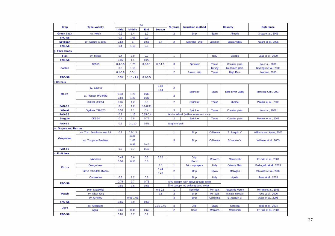
Table 4. Crop coefficient, Kc, values reported by the bibliographies and Kc FAO values.
26 Broad bean 0.37 1.05 Jordan Jordan Valley Amayreh and Al-Abed, 2003
FAO-56 0.5 1.15 1.1
Initial Middle End Season
a. Small vegetable
Cauliflower B. oleacea L. var. botrytis 0.84 1Red Cabbage B. oleacea L. var.rubra 0.83 1
FAO-56 1.05 0.95
cv. California Early 0.8 1.2-1.3 0.7 1cv. Chinese 0.91-0.94 1
FAO-56 1 0.7
Lettuce var. Capitata cv. XP 6256 0.3 0.6 1 Drip Chile Santiago Manuel-Casanova et al., 2009
FAO-56 1 0.95
Onion cv. Granero 0.65 1.2 0.75 1 Sprinkler Spain Albacete Lopez-Urrea et al., 2009
FAO-56 1 0.75
b. Vegetables – Solanum Family (Solanaceae)
0.6 1.15 0.8 2 Furrow Chile Maule region Ortega-Farias et al., 2006cv. Pull 1.1 1.3 0.8 1
Ibrido PS 1296 0.8 1.2 0.9 1
0.81 0.440.83 0.47 0.7
0.36 0.77-1.2 0.74 Drip Algeria Bechar, Tamanrasset Hamidat et al., 2002
Processing Tomato 0.19 0.99-1.08 0.6 4 Drip California Hanson and May, 20050.19 0.9-1.15 0.7 2 Drip with mulch Spain Ebro Valley Vazquez et al., 2005
FAO-56 1.15-1.2 0.7-0.9
Sweet pepper cv. Drago Lamuyo type 0.2 1.3 0.9 2 Drip Spain Almeria Orgaz et al., 2005
FAO-56 1.05 0.9
c. Vegetables - Cucumber Family (Cucurbitaceae)
cv. Categorìa (supported) 0.2 1.1 1 2cv. Eros Galia type (not supp.) 0.2 1.3 1.1 1
0.1 0.75 0.5 Drip whit mulch
0.15 0.85 0.6 Drip whitout mulch
FAO-56 1.05 0.75
Watermelon cv. Reina de Corazones 0.2 1.1 1 1 Drip Spain Almeria Orgaz et al., 2005
FAO-56 0.4 1 0.75
d. Roots and Tubers
0.870.85
FAO-56 1.15 0.75
e. Legumes
1.28
1.17
FAO-56 0.4 1.05 0.6-0.35
Tomato
Type-variety
var. Inodorus, cv. Nabucco
cv Desirée class AA1
CropKc
Melon
Garlic
DeTar, 2009Subsurface dripCowpea
Ferreira and Carr, 2002
California San Joaquin Valley
Portugal Braganca2Potato
Lovelli et al., 2005
Sprinkler
2
Amayreh and Al-Abed, 2005
Orgaz et al., 2005
Drip with mulch
Italy Basilicata
Jordan
Spain
Villalobos et al., 2004
Italy Puglia
Ponding Shin et al., 2009
Drip
SpainCenter-pivotGuadalquivir V. (Cordoba,Ecja)
Country
Turkey Erzurum
N. years Irrigation method
2
Almeria
2
Drip
Jordan Valley
California Blackeye N.46
Reference
Rinaldi and Rana, 2004
27
Initial Middle End Season
Green bean cv. Helda 0.2 1.4 1.2 2 Drip Spain Almeria Orgaz et al., 2005
FAO-56 0.5 1.05 0.9
Soybean cv. Asgrow A-3803 0.62 1 0.66 0.7 2 Sprinkler -Drip Lebanon Bekaa Valley Karam et al., 2005
FAO-56 0.4 1.15 0.5
g. Fibre Crops
Flax cv. Mikael 0.4 0.9 0.2 1 Italy Viterbo Casa et al., 2000
FAO-56 0.35 1.1 0.25
DP555 0.4-0.5 1.25 0.6-0.1 0.2-1.5 3 Sprinkler Texas Coastier plain Ko et al., 20090.8 1.13 1 Turkey Menemen plain Beyazigul et al., 2000
0.1-0.9 0.5-1 2 Furrow, drip Texas High Plain Lascano, 2000
FAO-56 0.35 1.15 - 1.2 0.7-0.5
i. Cereals0.88
0.940.48 1.28 0.350.59 1.27 0.35
32H39, 30G54 0.35 1.2 0.9 2 Sprinkler Texas Uvalde Piccinni et al., 2009
FAO-56 0.3 1.2 0.6-0.35
Wheat Ogallala, TAM203 0.53 1.1 0.4 3 Sprinkler Texas Coastier plain Ko et al., 2009
FAO-56 0.7 1.15 0.25-0.4 Winter Wheat (with non-fronzen soils)
Sorgum DKS 54 0.4 0.8 0.75 2 Sprinkler Texas Coastier plain Piccinni et al., 2009
FAO-56 0.3 1-1.10 0.55 Sorghum grain
m. Grapes and Berriescv. Tom. Seedless clone 2A 0.2 0.9-1.3 1 Drip California S. Joaquin V. Williams and Ayars, 2005
0.871.08
0.98 0.45
FAO-56 0.3 0.7 0.45
n. Fruit tree0.45 0.6 0.5 0.52 Drip 0.58 0.55 0.6 Flood
Orange tree 0.8 1 Micro-sprayers Italy Catania Plain Barbagallo et al., 20090.440.43
Clementine 0.8 1.2 0.8 1 Drip Italy Apulia Rana et al., 2005
0.75 0.7 0.75 70% canopy, with active ground cover0.65 0.6 0.65 50% canopy, no active ground cover
(var. Maybelle) 0.6-0.5 1 Sprinkler Portugal Aguas de Moura Ferreira et al., 1996 cv. Silver King 0.5 2 Drip Portugal Atalaia, Montijo Paço et al., 2006
cv. O'Henry 0.98-1.06 3 Drip California S. Joaquin V. Ayars et al., 2003
FAO-56 0.55 0.9 0.65
cv. Arbequino 0.35-0.45 3 Drip Spain Cordoba Testi et al., 2004
Agdal 0.65 0.45 0.65 2 Flood Morocco Marrakech Er-Raki et al., 2008
FAO-56 0.65 0.7 0.7
Crop Type-varietyKc
N. years Irrigation method Country
CitrusCitrus reticulata Blanco
Olive
cv. Tompson Seedless
cv. Pioneer PR34N43
Cotton
Marrakech
California S.Joaquin V.
Morocco
Drip
Reference
Sprinkler Martinez-Cob , 2007Maize
Spain Ebro River Valley2
2cv. Juanita
3
Er-Raki et al., 2009
Grapevine
Villalobos et al., 2009Spain Mazagon
Mandarin
Williams et al., 2003
2 Drip
Peach
FAO-56

Table 5. Basal crop coefficient, Kcb, values reported in review and Kcb values reported in FAO Paper 56
Initial Middle End Season
a. Small vegetable
Onion cv. Granero 0.6 1 0.65 1 Sprinkler Spain Albacete Lopez-Urrea et al., 2009
FAO-56 0.95 0.65
g. Fibre Crops
Flax cv. Mikael 0.7 1.1 0.2 1 Italy Viterbo Casa et al., 2000
FAO-56 1.05 0.2
j. Forages
Alfalfa 0.71 1.78 1.51 3 Sprinkler Turkey Plateau Anatolian Benli et al., 2006
FAO-56 0.3 1.15 1.1
n. Fruit tree
0.35 0.55 0.45 Drip
0.3 0.5 0.4 FloodFAO-56 0.6 0.55 0.6Peach cv. Silver King 0.7 0.66 2 Drip Portugal Atalaia, Montijo Paco et al., 2006
FAO-56 0.45 0.85 0.6
Crop Type-variety Kcb Country ReferenceN. years Irr.method
MarrakechCitrus Er-Raki et al., 2009Mandarin Morocco
28
Recommended