The Bright Side of Black Holes: RadiationFrom Black Hole Accretion Disks
The Harvard community has made thisarticle openly available. Please share howthis access benefits you. Your story matters
Citation Zhu, Yucong. 2015. The Bright Side of Black Holes: RadiationFrom Black Hole Accretion Disks. Doctoral dissertation, HarvardUniversity, Graduate School of Arts & Sciences.
Citable link http://nrs.harvard.edu/urn-3:HUL.InstRepos:17463143
Terms of Use This article was downloaded from Harvard University’s DASHrepository, and is made available under the terms and conditionsapplicable to Other Posted Material, as set forth at http://nrs.harvard.edu/urn-3:HUL.InstRepos:dash.current.terms-of-use#LAA
The Bright Side of Black Holes:
Radiation from Black Hole Accretion Disks
A dissertation presented
by
Yucong Zhu
to
The Department of Astronomy
in partial fulfillment of the requirements
for the degree of
Doctor of Philosophy
in the subject of
Astronomy & Astrophysics
Harvard University
Cambridge, Massachusetts
May 2015

©c 2015 — Yucong Zhu
All rights reserved.

Dissertation Advisor: Prof. Ramesh Narayan Yucong Zhu
The Bright Side of Black Holes:
Radiation from Black Hole Accretion Disks
Abstract
An understanding of radiation is paramount for connecting observations of accretion
disks with the theory of black holes. In this thesis, we explore via radiative transfer
postprocessing calculations the observational signatures of black holes. We investigate
disk spectra by analyzing general relativistic magnetohydrodynamic (GRMHD)
simulations of accretion disks. For the most part there are no surprises – the resulting
GRMHD spectrum is very close to the analytic Novikov & Thorne (1973) prediction
from decades past, except for a small modification in the case of spinning black holes,
which exhibit a high-energy power-law tail that is sourced by hot Comptonized gas from
within the plunging region of the accretion flow. These conclusions are borne out by
both 1D and 3D radiative transfer calculations of the disk. Significant effort was spent in
developing from scratch the 3D radiative code that we used for the analysis. The code is
named HERO (Hybrid Evaluator for Radiative Objects) and it is a new general purpose
grid-based 3D general relativistic radiative solver.
iii
Contents
Abstract iii
Acknowledgments ix
Dedication x
1 Introduction 1
1.1 Why Care About Black Holes? . . . . . . . . . . . . . . . . . . . . . . . . . 1
1.2 Mathematical Basis and Understanding . . . . . . . . . . . . . . . . . . . . 3
1.2.1 Kerr Metric . . . . . . . . . . . . . . . . . . . . . . . . . . . . . . . 3
1.2.2 Conservation Laws . . . . . . . . . . . . . . . . . . . . . . . . . . . 5
1.2.3 Metric Singularities . . . . . . . . . . . . . . . . . . . . . . . . . . . 6
1.2.4 Ergosphere . . . . . . . . . . . . . . . . . . . . . . . . . . . . . . . 9
1.2.5 Circular Orbits . . . . . . . . . . . . . . . . . . . . . . . . . . . . . 11
1.3 Observational Evidence for Black Holes . . . . . . . . . . . . . . . . . . . . 15
1.3.1 Spin Fitting Techniques . . . . . . . . . . . . . . . . . . . . . . . . 19
1.3.2 Zoology of Disk States . . . . . . . . . . . . . . . . . . . . . . . . . 22
1.4 Disk physics . . . . . . . . . . . . . . . . . . . . . . . . . . . . . . . . . . . 27
1.4.1 Classic Thin Disk Model . . . . . . . . . . . . . . . . . . . . . . . . 28
1.4.2 Relativistic Disk Model (Novikov & Thorne 1973) . . . . . . . . . . 32
1.4.3 Open problems in Accretion Physics . . . . . . . . . . . . . . . . . 34
iv
CONTENTS
1.5 Numerical Simulations . . . . . . . . . . . . . . . . . . . . . . . . . . . . . 36
1.5.1 Shearing Boxes . . . . . . . . . . . . . . . . . . . . . . . . . . . . . 38
1.5.2 Global Simulations . . . . . . . . . . . . . . . . . . . . . . . . . . . 39
1.5.3 Future Directions . . . . . . . . . . . . . . . . . . . . . . . . . . . . 40
1.6 Including Radiation . . . . . . . . . . . . . . . . . . . . . . . . . . . . . . . 41
1.6.1 Radiation Hydrodynamics . . . . . . . . . . . . . . . . . . . . . . . 42
1.7 Chapter Summaries . . . . . . . . . . . . . . . . . . . . . . . . . . . . . . . 45
2 The Eye of the Storm:
Light from the Inner Plunging Region of Black Hole Accretion Discs 49
2.1 Introduction . . . . . . . . . . . . . . . . . . . . . . . . . . . . . . . . . . . 50
2.2 GRMHD Simulations . . . . . . . . . . . . . . . . . . . . . . . . . . . . . . 57
2.3 Annuli Spectra . . . . . . . . . . . . . . . . . . . . . . . . . . . . . . . . . 58
2.3.1 Assumptions in the TLUSTY model . . . . . . . . . . . . . . . . . 61
2.4 Slicing the GRMHD disc into Annuli . . . . . . . . . . . . . . . . . . . . . 62
2.4.1 Flux profile . . . . . . . . . . . . . . . . . . . . . . . . . . . . . . . 64
2.4.2 Vertical gravity profile . . . . . . . . . . . . . . . . . . . . . . . . . 68
2.4.3 Column density profile . . . . . . . . . . . . . . . . . . . . . . . . . 69
2.5 Ray Tracing . . . . . . . . . . . . . . . . . . . . . . . . . . . . . . . . . . . 73
2.6 Results . . . . . . . . . . . . . . . . . . . . . . . . . . . . . . . . . . . . . . 76
2.6.1 Power law tail . . . . . . . . . . . . . . . . . . . . . . . . . . . . . . 78
2.6.2 Quantitative effect on spin . . . . . . . . . . . . . . . . . . . . . . . 83
2.7 Discussion . . . . . . . . . . . . . . . . . . . . . . . . . . . . . . . . . . . . 91
2.7.1 Other signatures of the plunging region . . . . . . . . . . . . . . . . 95
2.7.2 How does our choice of cooling function influence the results? . . . 96
2.7.3 Equation of state . . . . . . . . . . . . . . . . . . . . . . . . . . . . 98
2.8 Summary . . . . . . . . . . . . . . . . . . . . . . . . . . . . . . . . . . . . 99
v

CONTENTS
2.9 Luminosity Matching Model . . . . . . . . . . . . . . . . . . . . . . . . . . 101
2.10 Generalized Novikov & Thorne Model . . . . . . . . . . . . . . . . . . . . . 102
2.11 Interpolation Methods . . . . . . . . . . . . . . . . . . . . . . . . . . . . . 105
2.12 An Alternative GRMHD Luminosity Profile . . . . . . . . . . . . . . . . . 108
2.12.1 Obtaining the GRMHD dissipation profile . . . . . . . . . . . . . . 110
2.12.2 Net result of the luminosity calculation . . . . . . . . . . . . . . . . 110
3 Thermal Stability in Turbulent Accretion Discs 113
3.1 Introduction . . . . . . . . . . . . . . . . . . . . . . . . . . . . . . . . . . . 114
3.2 Physical model . . . . . . . . . . . . . . . . . . . . . . . . . . . . . . . . . 117
3.2.1 Radial structure . . . . . . . . . . . . . . . . . . . . . . . . . . . . . 118
3.2.2 Vertical structure . . . . . . . . . . . . . . . . . . . . . . . . . . . . 119
3.3 Disc solutions . . . . . . . . . . . . . . . . . . . . . . . . . . . . . . . . . . 126
3.3.1 Classic unmixed disc . . . . . . . . . . . . . . . . . . . . . . . . . . 128
3.3.2 Convective solutions . . . . . . . . . . . . . . . . . . . . . . . . . . 131
3.3.3 Convective and turbulent disc solutions . . . . . . . . . . . . . . . . 133
3.3.4 Radial structure of solutions . . . . . . . . . . . . . . . . . . . . . . 139
3.4 Discussion . . . . . . . . . . . . . . . . . . . . . . . . . . . . . . . . . . . . 144
3.4.1 Use of logarithmic temperature gradient . . . . . . . . . . . . . . . 145
3.4.2 Impact of Σscale . . . . . . . . . . . . . . . . . . . . . . . . . . . . . 148
3.4.3 Scaling of Critical M with Black Hole Mass . . . . . . . . . . . . . 149
3.4.4 Choosing ζ – comparison with simulations . . . . . . . . . . . . . . 151
3.4.5 ζ from observations . . . . . . . . . . . . . . . . . . . . . . . . . . . 158
3.4.6 Radiative Outer Zone . . . . . . . . . . . . . . . . . . . . . . . . . . 158
3.4.7 Complete stabilization from turbulence . . . . . . . . . . . . . . . . 162
3.5 Summary . . . . . . . . . . . . . . . . . . . . . . . . . . . . . . . . . . . . 165
3.6 Acknowledgments . . . . . . . . . . . . . . . . . . . . . . . . . . . . . . . . 166
vi
CONTENTS
3.7 Solving for 8 unknowns . . . . . . . . . . . . . . . . . . . . . . . . . . . . . 167
4 HERO - A 3D General Relativistic Radiative Postprocessor for Accre-
tion Discs around Black Holes 170
4.1 Introduction . . . . . . . . . . . . . . . . . . . . . . . . . . . . . . . . . . . 171
4.2 Radiative Solver . . . . . . . . . . . . . . . . . . . . . . . . . . . . . . . . . 176
4.2.1 Short Characteristics . . . . . . . . . . . . . . . . . . . . . . . . . . 178
4.2.2 Implementation of Short Characteristics . . . . . . . . . . . . . . . 183
4.2.3 Long Characteristics . . . . . . . . . . . . . . . . . . . . . . . . . . 185
4.2.4 Acceleration Schemes . . . . . . . . . . . . . . . . . . . . . . . . . . 188
4.2.5 Raytracing . . . . . . . . . . . . . . . . . . . . . . . . . . . . . . . . 190
4.2.6 Frequency Discretization . . . . . . . . . . . . . . . . . . . . . . . . 191
4.2.7 Angular Discretization . . . . . . . . . . . . . . . . . . . . . . . . . 191
4.3 Numerical Tests . . . . . . . . . . . . . . . . . . . . . . . . . . . . . . . . . 194
4.3.1 1D Plane-parallel Grey Atmosphere . . . . . . . . . . . . . . . . . . 195
4.3.2 Convergence Tests . . . . . . . . . . . . . . . . . . . . . . . . . . . 197
4.3.3 Multiray Temperature Solution . . . . . . . . . . . . . . . . . . . . 198
4.3.4 Test of Spectral Hardening . . . . . . . . . . . . . . . . . . . . . . . 200
4.3.5 Effect of a Heating Source . . . . . . . . . . . . . . . . . . . . . . . 201
4.3.6 2D Solutions and Ray Defects . . . . . . . . . . . . . . . . . . . . . 204
4.3.7 3D Solutions . . . . . . . . . . . . . . . . . . . . . . . . . . . . . . . 209
4.3.8 GR Solutions . . . . . . . . . . . . . . . . . . . . . . . . . . . . . . 216
4.4 Summary . . . . . . . . . . . . . . . . . . . . . . . . . . . . . . . . . . . . 228
4.5 Acknowledgements . . . . . . . . . . . . . . . . . . . . . . . . . . . . . . . 229
4.6 Ray Defects . . . . . . . . . . . . . . . . . . . . . . . . . . . . . . . . . . . 230
4.6.1 Mathematical Origin of Ray Defects . . . . . . . . . . . . . . . . . 233
4.6.2 Ray Defect Correction Schemes . . . . . . . . . . . . . . . . . . . . 235
vii
CONTENTS
4.7 Analytic 1D Atmosphere Spectrum . . . . . . . . . . . . . . . . . . . . . . 238
5 HEROIC - A Comptonization Module for the HERO radiative code 242
5.1 Introduction . . . . . . . . . . . . . . . . . . . . . . . . . . . . . . . . . . . 243
5.2 Radiative Transfer Solution . . . . . . . . . . . . . . . . . . . . . . . . . . 246
5.2.1 Kompaneets-Ray . . . . . . . . . . . . . . . . . . . . . . . . . . . . 248
5.2.2 Quadratic Variation of the Source Function . . . . . . . . . . . . . 250
5.3 Numerical Tests . . . . . . . . . . . . . . . . . . . . . . . . . . . . . . . . . 253
5.3.1 Kompaneets . . . . . . . . . . . . . . . . . . . . . . . . . . . . . . . 253
5.3.2 Escape Time Distributions . . . . . . . . . . . . . . . . . . . . . . . 256
5.4 Application – Accretion Disk . . . . . . . . . . . . . . . . . . . . . . . . . . 264
5.4.1 Numerical Disk Setup . . . . . . . . . . . . . . . . . . . . . . . . . 265
5.4.2 Results . . . . . . . . . . . . . . . . . . . . . . . . . . . . . . . . . . 267
5.5 Discussion . . . . . . . . . . . . . . . . . . . . . . . . . . . . . . . . . . . . 274
5.6 Summary . . . . . . . . . . . . . . . . . . . . . . . . . . . . . . . . . . . . 280
6 Summary and Future Directions 282
6.1 Summary . . . . . . . . . . . . . . . . . . . . . . . . . . . . . . . . . . . . 282
6.2 Future Directions . . . . . . . . . . . . . . . . . . . . . . . . . . . . . . . . 284
6.2.1 Astrophysical Applications . . . . . . . . . . . . . . . . . . . . . . . 284
6.2.2 Future Plans for HERO . . . . . . . . . . . . . . . . . . . . . . . . 285
References 288
viii

Acknowledgments
I thank my advisor, Ramesh Narayan, for his boundless insights, and endless
patience.
I thank my friends, for bringing so much joy to my life.
I thank my family, for all their love, support, and encouragement throughout the
years.
ix

For my fellow travelers in space and time.
x

Chapter 1
Introduction
1.1 Why Care About Black Holes?
Our universe can be thought of as a gigantic all encompassing house – every material
thing that we know of (matter and energy) lives inside of it. Just like a human domicile,
the universe burns fuel (stars) to keep warm, releasing tremendous amounts of radiative
energy before burning out, leaving only a dark ash behind; in the case of stars, the ash
is comprised of compact objects such as white dwarfs, neutron stars, or black holes,
depending on the mass of the stellar progenitor.
Black holes are perhaps the most exciting of these three destinations of stellar
evolution. They are more than just ash – when conditions are right (e.g., under the
influence of gas accretion), a black hole can become a phoenix. It rises from the ashes
to light up the universe anew with unimaginable luminosity, producing at the same time
tremendous jets that are powerful enough to shape and govern the evolution of galaxies!
1

CHAPTER 1. INTRODUCTION
Even more remarkable is the efficiency at which black holes convert matter into
energy. Due to their extreme gravity, the accretion process (and the subsequent
dissipation of gravitational potential energy) leads to the extraction of rest mass energy
at an efficiency of 10-100 times higher1 than that of even nuclear fusion! Hence black
holes can be thought of as the true powerplants of our universe, and therefore crucial
to understanding the evolution and fate of our universe (e.g. AGN feedback on galactic
dynamics, dominating the epoch of reionization, and dictating the physics of the most
violent explosions in the universe).
Perhaps the most interesting aspect of black holes lies in their extremal nature.
Space and time become intimately and infinitely mixed at the surface of a black hole,
which provides the ultimate testbed for our physical theories of gravity. It is only near
the event horizon2 of a black hole where general relativity (our current best-guess on the
inner workings of gravity) can truly be put to the test.
Black holes are the ultimate triumph of modern astrophysics. They were originally
predicted from purely mathematical arguments, only to be later verified observationally
in the 1970’s by X-ray observations of accreting stellar binaries and in the 1990s by
high angular resolution optical and infrared observations of galactic nuclei. They have
a profound influence on our universe and are also objects of immense mathematical
simplicity and beauty.
1The mass-energy conversion efficiency depends on the spin of the black hole, whereby high spin leads
to higher efficiencies
2The event horizon is the surface at which gravity becomes so strong that light itself cannot escape
its wretched pull
2
CHAPTER 1. INTRODUCTION
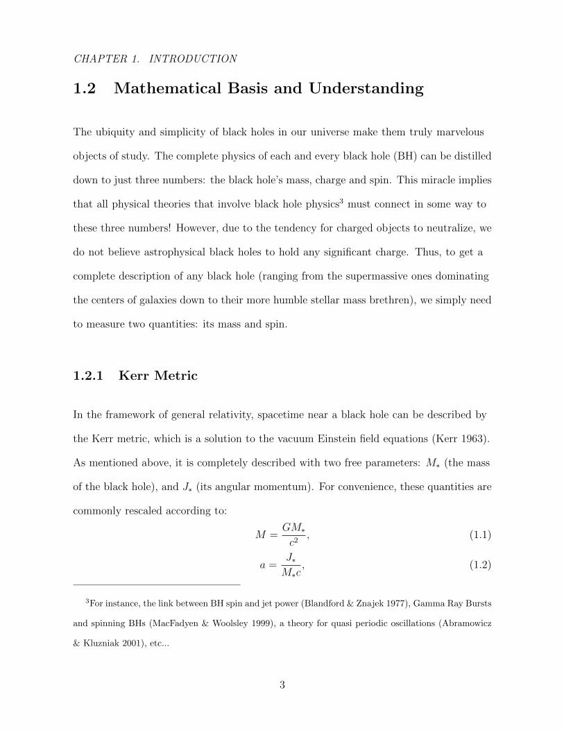
1.2 Mathematical Basis and Understanding
The ubiquity and simplicity of black holes in our universe make them truly marvelous
objects of study. The complete physics of each and every black hole (BH) can be distilled
down to just three numbers: the black hole’s mass, charge and spin. This miracle implies
that all physical theories that involve black hole physics3 must connect in some way to
these three numbers! However, due to the tendency for charged objects to neutralize, we
do not believe astrophysical black holes to hold any significant charge. Thus, to get a
complete description of any black hole (ranging from the supermassive ones dominating
the centers of galaxies down to their more humble stellar mass brethren), we simply need
to measure two quantities: its mass and spin.
1.2.1 Kerr Metric
In the framework of general relativity, spacetime near a black hole can be described by
the Kerr metric, which is a solution to the vacuum Einstein field equations (Kerr 1963).
As mentioned above, it is completely described with two free parameters: M∗ (the mass
of the black hole), and J∗ (its angular momentum). For convenience, these quantities are
commonly rescaled according to:
M =GM∗c2
, (1.1)
a =J∗M∗c
, (1.2)
3For instance, the link between BH spin and jet power (Blandford & Znajek 1977), Gamma Ray Bursts
and spinning BHs (MacFadyen & Woolsley 1999), a theory for quasi periodic oscillations (Abramowicz
& Kluzniak 2001), etc...
3
CHAPTER 1. INTRODUCTION
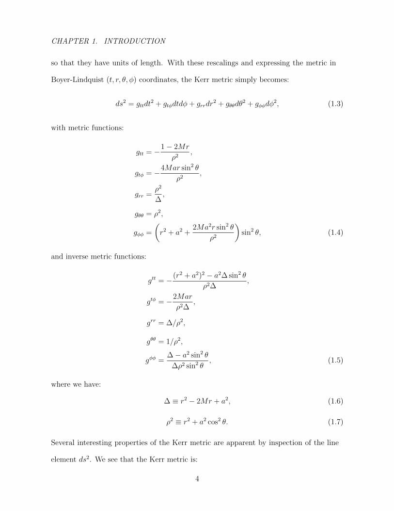
so that they have units of length. With these rescalings and expressing the metric in
Boyer-Lindquist (t, r, θ, φ) coordinates, the Kerr metric simply becomes:
ds2 = gttdt2 + gtφdtdφ+ grrdr
2 + gθθdθ2 + gφφdφ
2, (1.3)
with metric functions:
gtt = −1− 2Mr
ρ2,
gtφ = −4Mar sin2 θ
ρ2,
grr =ρ2
∆,
gθθ = ρ2,
gφφ =
(r2 + a2 +
2Ma2r sin2 θ
ρ2
)sin2 θ, (1.4)
and inverse metric functions:
gtt = −(r2 + a2)2 − a2∆ sin2 θ
ρ2∆,
gtφ = −2Mar
ρ2∆,
grr = ∆/ρ2,
gθθ = 1/ρ2,
gφφ =∆− a2 sin2 θ
∆ρ2 sin2 θ, (1.5)
where we have:
∆ ≡ r2 − 2Mr + a2, (1.6)
ρ2 ≡ r2 + a2 cos2 θ. (1.7)
Several interesting properties of the Kerr metric are apparent by inspection of the line
element ds2. We see that the Kerr metric is:
4
CHAPTER 1. INTRODUCTION
• stationary: it does not depend explicitly on time t.
• axisymmetric: it does not depend explicitly on φ.
• invariant under simultaneous inversion of t and φ (i.e. t → −t and φ → −φ). A
rotating object also produces this symmetry, motivating the link between rotation
and the Kerr metric.
• Minkowski (i.e. special-relativistic flat space) in the limit r → ∞, hence Kerr
spacetime is asymptotically flat.
• Schwarzchild in the limit a→ 0.
• Minkowski in the limit M → 0 (even with a 6= 0).
We explore the implications of these properties and draw additional insights from
the mathematical structure of the metric in the next few subsections.
1.2.2 Conservation Laws
From Noether’s theorem (Noether 1918), one expects conservation laws to be associated
with symmetries within a system. The Kerr metric is independent of both time t and
azimuth φ and is hence symmetric in translations about these coordinates. This allows
one to define a set of orthogonal “Killing” vectors that point along directions that leave
the metric unchanged, i.e.
ηµ = δµt, (1.8)
ξµ = δµφ. (1.9)
5
CHAPTER 1. INTRODUCTION
A Killing vector is a general way of characterizing the symmetry in a given coordinate
system. It has the property that its inner product with a particle/photon’s four-
momentum pµ is conserved along geodesics. This gives rise to the notion of energy and
angular momentum conservation corresponding to the two symmetries/Killing vectors
present:
energy : E = −ηµpµ = −pt (1.10)
, angular momentum : L = ξµpµ = pφ. (1.11)
For massive particles the four-momentum corresponds to pµ = muµ, and the conserved
quantities E , L correspond to the per unit mass energy and angular momentum
respectively. For massless photons, an affine invariant can be chosen such that the
four-momentum becomes pµ = uµ, leading to the conserved quantities E , L representing
the photon’s energy and angular momentum as measured at infinity.
The two Killing vectors ηµ and ξµ also span all available Killing vector fields present
in the Kerr metric. Any other Killing vector can be expressed as a linear combination of
these two. 4:
1.2.3 Metric Singularities
The metric as defined in Eq. 1.3 becomes singular on the submanifolds
0 = ρ2 = r2 + a2 cos2 θ, (1.12)
4A third symmetry also exists within the Kerr metric, though it is generated via a more complex
Killing tensor field Kµν . This gives rise to a third conserved quantity, the Carter constant C =
Kµνpµpν = (pθ)2 + (pφ)2/ sin2(θ) = const, which describes the mix of poloidal and toroidal momentum
that is conserved during particle motion.
6

CHAPTER 1. INTRODUCTION
or
0 = ∆ = r2 − 2Mr + a2. (1.13)
Of these two, only the first condition ρ2 → 0 corresponds to a true curvature singularity
(i.e. as verified by evaluating the scalar curvature invariant RαβγδRαβγδ → ∞). It
corresponds to the coordinates r = 0 and θ = π/2, although mapping these coordinates
to the usual Boyer-Lindquist/spherical-polar sense leaves some confusion since r = 0 also
corresponds to a coordinate singularity. Under a transformation to a new coordinate
system (i.e. Kerr-Schild which does not suffer from the r = 0 coordinate singularity), the
topological nature of the curvature singularity is revealed to be a thin ring. The radius
of the ring-singularity is set by the spin of the black hole, vanishing to a point-singularity
in the limit of a nonrotating black hole (a = 0).
∆→ 0 corresponds to a coordinate singularity that can be dealt with by means of a
coordinate transformation. Kerr coordinates is one such one that regularizes the ∆→ 0
condition, and is motivated by using null-worldlines to define a new time-basis (i.e. in a
similar fashion as Eddington-Finkelstein coordinates).
An interesting feature of the ∆ = 0 submanifold is its quadratic nature. Two
solutions exist for the condition ∆ = 0, corresponding to “inner” and “outer” singularities
and are located at
0 = r2 − 2Mr + a2 = (r − r+)(r − r−) (1.14)
⇒ r± = M ±√M2 − a2. (1.15)
The interpretation of this ∆ = 0 surface can be motivated by considering the
Schwarzschild a = 0 case. Here we have r+ = 2M , which corresponds to the location
7
CHAPTER 1. INTRODUCTION
of the classic black hole event horizon. Thus, we identify r± as the outer and inner
horizons of a spinning black hole, with the outer horizon r+ serving as the boundary that
separates the causally connected exterior Universe from the Kerr interior.
Alternatively, a more mathematically rigorous way of interpreting the r = r±
hypersurfaces is to consider the radial surface normal four-vector, i.e. in Boyer-Lindquist
(t, r, θ, φ):
nα = (0, 1, 0, 0). (1.16)
By examining the inner product of nα, we can characterize the normal vector. Note that
nαnα = nαnβg
αβ = grr =∆
ρ2(1.17)
and therefore the normal vectors along the ∆ = 0 surface have nαnα = 0 (null-like).
Hence r = r± are horizons since the light cone collapses to the radial vector here. The
two horizons also separate space into three distinct subregions, whose properties can
be further explored by consideration of the tangent vector field along constant radius
surfaces (Misner, Thorne, & Wheeler 1973; D’Inverno 1992):
• r > r+: This region represents the exterior of the black hole, becoming flat
spacetime in the limit r → ∞. Here, constant radius surfaces have tangent fields
that are timelike, and therefore non-descending worldlines are accessible.
• r− < r < r+: This is the region between the two horizons. Tangent vectors for
constant radius surfaces are spacelike, and therefore all valid worldlines must
descend towards smaller radius. Eventually all material in this zone is channeled
inwards and falls through the inner horizon.
• r < r−: This is the innermost region containing the ring singularity as discussed
8

CHAPTER 1. INTRODUCTION
above. Tangent bundles on radial surfaces are once again timelike and the worldline
restriction on radial monotonicity is lifted here.
Finally note that whenever a > M , the equation ∆ = 0 has no real solution,
implying the absence of a horizon and leaving the Kerr singularity at ρ2 = 0 “not
covered” by a horizon, resulting in a “naked singularity” that is exposed and accessible to
the rest of the Universe. Due to the strange nature of spacetime around the singularity
(i.e. causality paradoxes), this situation is considered unphysical, and it is believed that
all astrophysical black holes in the universe are constrained to have a ≤M .5
1.2.4 Ergosphere
An interesting property of the Kerr spacetime is that relativistic “frame-dragging” effects
due to black hole rotation prevents the existence of stationary observers close to the
black hole. This property can be easily deduced by considering the four-normal of a
stationary observer, i.e.
ηµ = (1, 0, 0, 0). (1.18)
To check whether this time-stationary worldline is valid, we proceed like in the previous
section on horizons – we compute its inner product to classify whether it is either timelike
5The limiting case of a = M is typically referred to as an extremal black hole.
9
CHAPTER 1. INTRODUCTION
or spacelike to determine if it is a valid observer worldline:
ηµηµ = gµνη
µην = gtt
= −1 +2Mr
ρ2= − 1
ρ2
(r2 − 2Mr + a2 cos2 θ
)= − 1
ρ2(r − rE+) (r − rE−) , (1.19)
where the function roots are located at
rE± = M ±√M2 − a2 cos2 θ. (1.20)
Once again, due to the quadratic nature of Eq. 1.19, the two roots subdivide space
into three regions. Of particular interest is the subregion rE− < r < rE+ known as
the “ergosphere”, where gtt = ηµηµ > 0 indicating that the stationary observer has an
unphysical spacelike worldline. Thus, in this region a stationary observer with fixed
(r, θ, φ) cannot exist. This ergosphere constitutes a portion of space where the rotational
influence of the black hole is so violent that it is impossible to remain fixed in space – in
the ergosphere, all material is forced to rotate in the same sense as the black hole.
The manifold spanned by rE± also enjoys the distinction of being infinite redshift
surfaces. That is, any source located on this surface emits light signals that are
suppressed by a factor:
νobs =
√gemittt
gobstt
νemit, (1.21)
and since gemittt = 0, the photon is redshifted to oblivion when measured by another
nonlocal observer.
Finally, notice that the topology of the twin gtt null surfaces are simply ellipsoids
in Boyer-Lindquist coordinates. The boundary of the ergoregion given by Eq. 1.20 also
10
CHAPTER 1. INTRODUCTION
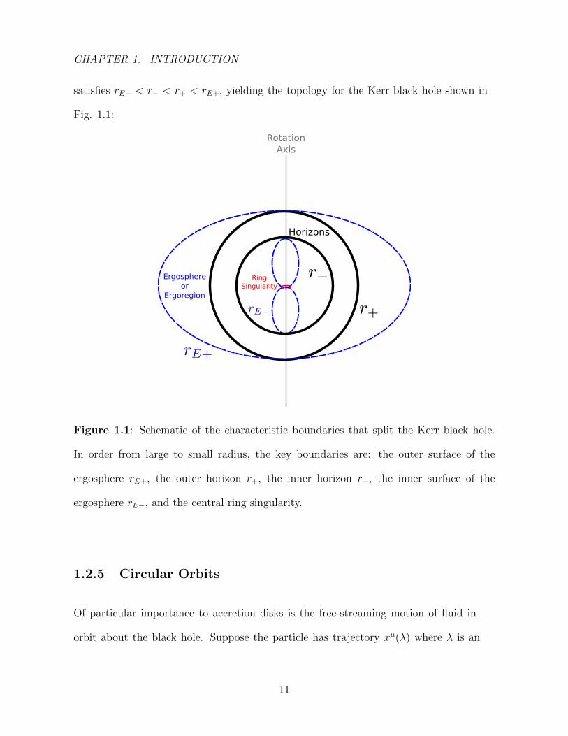
satisfies rE− < r− < r+ < rE+, yielding the topology for the Kerr black hole shown in
Fig. 1.1:
RingSingularity
RotationAxis
Horizons
Ergosphereor
Ergoregion
Figure 1.1: Schematic of the characteristic boundaries that split the Kerr black hole.
In order from large to small radius, the key boundaries are: the outer surface of the
ergosphere rE+, the outer horizon r+, the inner horizon r−, the inner surface of the
ergosphere rE−, and the central ring singularity.
1.2.5 Circular Orbits
Of particular importance to accretion disks is the free-streaming motion of fluid in
orbit about the black hole. Suppose the particle has trajectory xµ(λ) where λ is an
11
CHAPTER 1. INTRODUCTION
affine parametrization of the particle’s path6, then in the framework of GR, this free
“geodesic” motion with say velocity uµ = dxµ/dτ is governed by trajectories with
vanishing acceleration, i.e.
0 = aµ = uν∇νuµ (1.22)
=d2xα
dτ 2+ Γαβγ
dxβ
dτ
dxγ
dτ(1.23)
where Γαβγ are the connection coefficients of the coordinate system7, given by
Γαβγ =1
2gακ(∂gβκ∂xγ
+∂gγκ∂xβ
− ∂gβγ∂xκ
). (1.24)
By consideration of the constants of motion E ,L as described in 1.2.2, and for the case of
motion in the equatorial plane (θ = π/2), Bardeen, Press, & Teukolsky (1972) deduced
simpler and decoupled forms corresponding to geodesic motion. The radial component
of the trajectory obeys:
ρ2 dr
dλ= ±V 1/2
r , (1.25)
where Vr defines an effective potential given by
Vr = T 2 −∆[µr2 + (L − aE)2] (1.26)
T = E(r2 + a2)− La, (1.27)
and µ = u · u is a switch that toggles between the case of massive particles (µ = 1) and
photons (µ = 0). For circular motion, we must have dr/dλ = 0 both instantaneously
and for all subsequent times (since r is constant for circular orbits), which from Eq.1.25
6The affine parameter λ is typically chosen as the proper time τ for massive particles and the proper
path length for massless particles
7see Appendix D of Chung (2010) for a full listing of nonzero connection coefficients in the Kerr metric
12

CHAPTER 1. INTRODUCTION
translates to the following conditions for the effective potential:
Vr = 0 and∂Vr
∂λ= 0 (1.28)
For a given radius r, the above constraints can be solved simultaneously, which sets the
required values of E and L. However, circular orbits do not exist for all values of r since
the solutions for E and L are real valued only under the condition
r3/2 − 3Mr ± 2aM1/2 ≥ 0. (1.29)
The limiting case of equality in Eq. 1.29 yields infinite energy per rest mass,
corresponding to the photon orbit, and is given by the root
rph = 2M
1 + cos
[2
3cos−1
(∓aM
)]. (1.30)
If one further demands that the circular orbit be stable, then we must also have V ′′r ≤ 0.
This translates into the condition
r2 − 6Mr ± 8aM1/2r1/2 − 3a2 ≥ 0 (1.31)
or r > rms where rms is the marginally stable orbit (alternatively, the “Innermost Stable
Circular Orbit”– ISCO). It is located at
rms = M
3 + Z2 ∓ [(3− Z1) (3 + Z1 + 2Z2)]1/2, (1.32)
Z1 ≡ 1 +(1− a2/M2
)1/3[(1 + a/M)1/3 + (1− a/M)1/3
]Z2 ≡
(3a2/M2 + Z 2
1
)1/2.
The ISCO is particularly relevant for accretion disks since it acts as a boundary that
separates two regimes of the accretion flow. When r > rms, the turbulent flow quickly
circularizes and follows Keplerian orbits about the black hole. Material is viscously
13
CHAPTER 1. INTRODUCTION
transported inwards and upon reaching r = rms suddenly switches from circular to nearly
radial free-fall. This transition leads to an inner truncation of the accretion disk at the
location of rms, and provides a strong observational signature for accretion flows about
black holes.
1.0 0.5 0.0 0.5 1.0a/M
0
1
2
3
4
5
6
7
8
9
r/M
retrograde prograde
rms
rph
max(rE +)
r+
r−
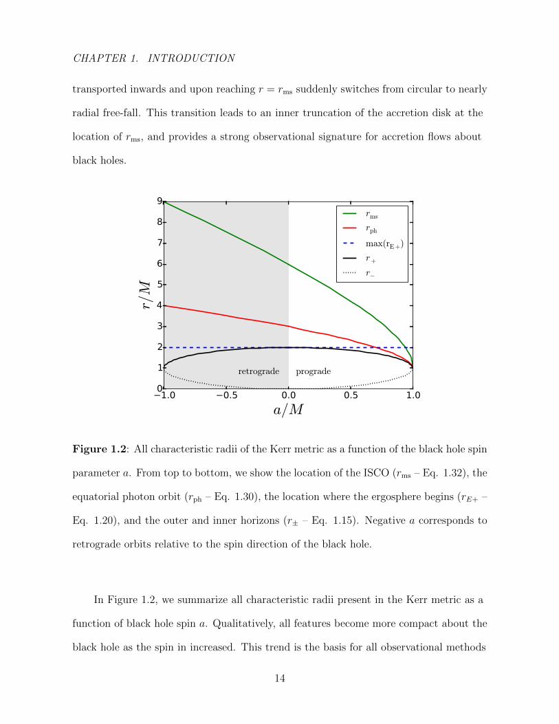
Figure 1.2: All characteristic radii of the Kerr metric as a function of the black hole spin
parameter a. From top to bottom, we show the location of the ISCO (rms – Eq. 1.32), the
equatorial photon orbit (rph – Eq. 1.30), the location where the ergosphere begins (rE+ –
Eq. 1.20), and the outer and inner horizons (r± – Eq. 1.15). Negative a corresponds to
retrograde orbits relative to the spin direction of the black hole.
In Figure 1.2, we summarize all characteristic radii present in the Kerr metric as a
function of black hole spin a. Qualitatively, all features become more compact about the
black hole as the spin in increased. This trend is the basis for all observational methods
14
CHAPTER 1. INTRODUCTION
that measure black hole spin (see §1.3.1 for details).
1.3 Observational Evidence for Black Holes
Black holes have been in the forefront of the imagination of both scientists and the
general public for nearly a century. Karl Schwarzchild originally proposed their existence
as a mathematical curiosity in 1916, and it was only much later that their link as the
final end product of astrophysical stellar collapse was made by Oppenheimer & Snyder
in 1939. Nevertheless, the long journey of gathering sufficient evidence to serve as
conclusive proof of black holes was only recently realized through careful obsevations of
stellar binary systems (Bolton 1972; Webster & Murdin 1972; McClintock & Remillard
1986).
Multiple lines of evidence are used to argue the case of black hole existence. For
instance in some binary systems, the observed millisecond flickering rate of several
X-ray binaries suggests the presence of a very compact primary object with size scales
comparable to the predicted size of black holes. Another hint comes from radial velocity
measurements of stellar companion – for some systems, the inferred lower limit on the
mass of the primary object exceeds 3M, the maximal limit allowed for neutron stars.
This combination of small spatial size and high mass rule out any other astrophysical
object except for a black hole. Similar mass and size constraint arguments have also
been made to argue for the existence of our Galaxy’s central supermassive black hole
(Genzel, Hollenbach & Townes 1994; Kormendy & Richstone 1995; Genzel, Eisenhauer
& Gillenssen 2010), as well as for many extragalactic supermassive black holes (e.g. M32
– van der Marel et al. 1997; M31 – Tonry 1984; NGC4526 – Miyoshi et al. 1995; and
15
CHAPTER 1. INTRODUCTION
many others – Kormendy & Ho 2014).
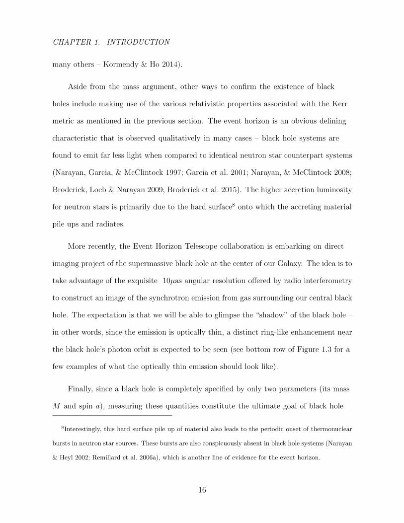
Aside from the mass argument, other ways to confirm the existence of black
holes include making use of the various relativistic properties associated with the Kerr
metric as mentioned in the previous section. The event horizon is an obvious defining
characteristic that is observed qualitatively in many cases – black hole systems are
found to emit far less light when compared to identical neutron star counterpart systems
(Narayan, Garcia, & McClintock 1997; Garcia et al. 2001; Narayan, & McClintock 2008;
Broderick, Loeb & Narayan 2009; Broderick et al. 2015). The higher accretion luminosity
for neutron stars is primarily due to the hard surface8 onto which the accreting material
pile ups and radiates.
More recently, the Event Horizon Telescope collaboration is embarking on direct
imaging project of the supermassive black hole at the center of our Galaxy. The idea is to
take advantage of the exquisite 10µas angular resolution offered by radio interferometry
to construct an image of the synchrotron emission from gas surrounding our central black
hole. The expectation is that we will be able to glimpse the “shadow” of the black hole –
in other words, since the emission is optically thin, a distinct ring-like enhancement near
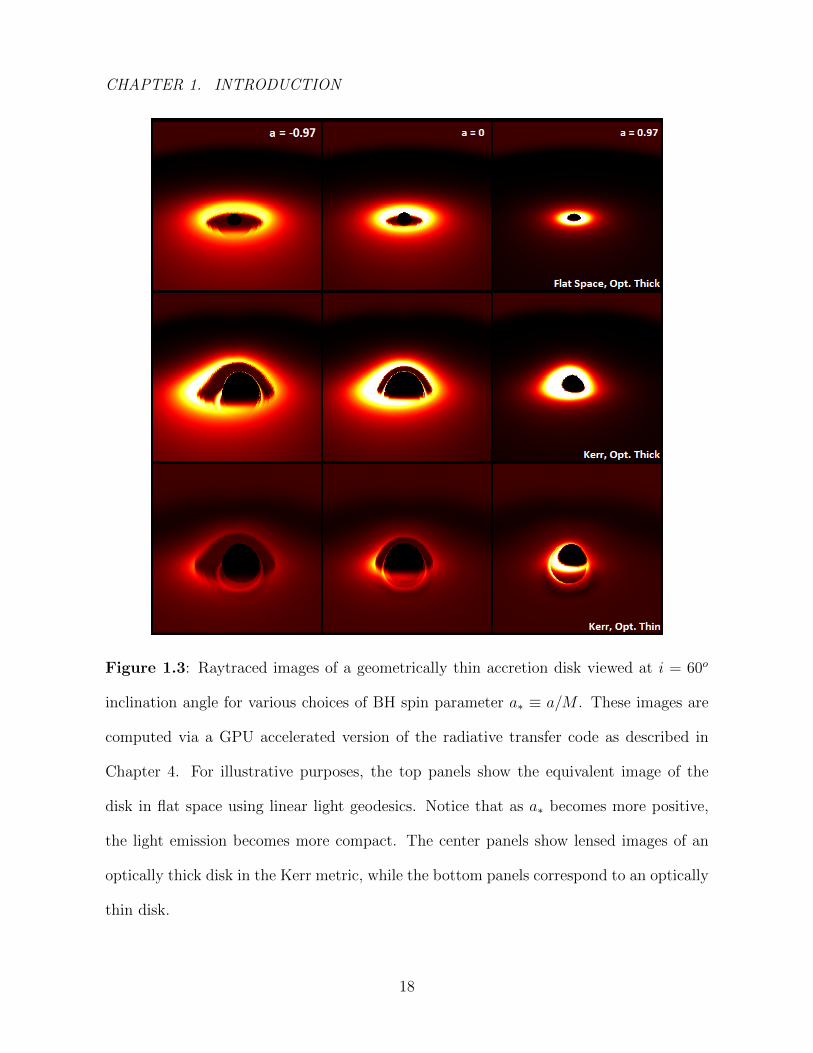
the black hole’s photon orbit is expected to be seen (see bottom row of Figure 1.3 for a
few examples of what the optically thin emission should look like).
Finally, since a black hole is completely specified by only two parameters (its mass
M and spin a), measuring these quantities constitute the ultimate goal of black hole
8Interestingly, this hard surface pile up of material also leads to the periodic onset of thermonuclear
bursts in neutron star sources. These bursts are also conspicuously absent in black hole systems (Narayan
& Heyl 2002; Remillard et al. 2006a), which is another line of evidence for the event horizon.
16
CHAPTER 1. INTRODUCTION
observations. Having these numbers will also inform us if our understanding of black hole
physics is correct (and by extension, test the theory of relativity in the strong gravity
limit). For binary systems, the task of measuring mass is relatively straightforward. So
long as one can accurately measure the inclination, period, and radial velocity for a
companion orbiting a black hole, one can immediately obtain the black hole mass as
direct consequence of Newtonian gravity. To date, over 20 mass measurements have been
made for stellar mass binary black holes (Remillard & McClintock 2006b), and over ∼ 50
for supermassive black holes (Gultekin et al. 2009).
Despite this success in the mass sector, spin has proven to be a much more difficult
quantity to pin down. The spin of the black hole only imprints its signature through
the general relativistic frame dragging effect, which only occurs at very short distances
(see discussion on Ergosphere in §1.2.4). Thus to probe black hole spin, we must rely
on observations of fluid that is very close to the BH horizon – namely the part of the
accretion disk orbiting close-in (i.e. see figure 1.3, which shows a few example raytraced
images of the accretion disk). Currently, there are two main techniques (see §1.3.1 for
details) that make use of the light from accretion disks to pin down BH spin. Both
techniques make use of the same underlying principle, which is to measure the location
of the innermost stable circular orbit (ISCO). As shown in Fig. 1.2, the ISCO size,
which can be determined by measuring the size of the dark central void, is a monotonic
function of black hole spin. It is through this ISCO size monotonicity relation that we
infer the spin (McClintock et al. 2011; McClintock, Narayan & Steiner 2014).
17
CHAPTER 1. INTRODUCTION
Figure 1.3: Raytraced images of a geometrically thin accretion disk viewed at i = 60o
inclination angle for various choices of BH spin parameter a∗ ≡ a/M . These images are
computed via a GPU accelerated version of the radiative transfer code as described in
Chapter 4. For illustrative purposes, the top panels show the equivalent image of the
disk in flat space using linear light geodesics. Notice that as a∗ becomes more positive,
the light emission becomes more compact. The center panels show lensed images of an
optically thick disk in the Kerr metric, while the bottom panels correspond to an optically
thin disk.
18
CHAPTER 1. INTRODUCTION
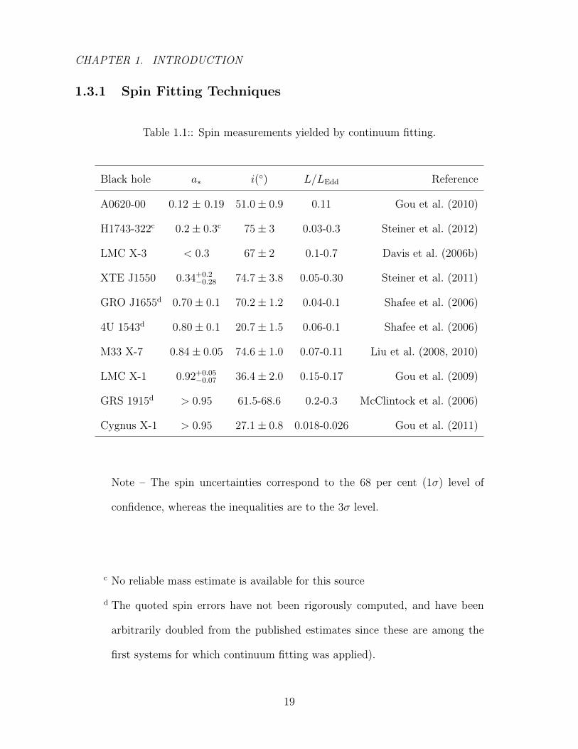
1.3.1 Spin Fitting Techniques
Table 1.1:: Spin measurements yielded by continuum fitting.
Black hole a∗ i() L/LEdd Reference
A0620-00 0.12 ± 0.19 51.0± 0.9 0.11 Gou et al. (2010)
H1743-322c 0.2± 0.3c 75± 3 0.03-0.3 Steiner et al. (2012)
LMC X-3 < 0.3 67± 2 0.1-0.7 Davis et al. (2006b)
XTE J1550 0.34+0.2−0.28 74.7± 3.8 0.05-0.30 Steiner et al. (2011)
GRO J1655d 0.70± 0.1 70.2± 1.2 0.04-0.1 Shafee et al. (2006)
4U 1543d 0.80± 0.1 20.7± 1.5 0.06-0.1 Shafee et al. (2006)
M33 X-7 0.84± 0.05 74.6± 1.0 0.07-0.11 Liu et al. (2008, 2010)
LMC X-1 0.92+0.05−0.07 36.4± 2.0 0.15-0.17 Gou et al. (2009)
GRS 1915d > 0.95 61.5-68.6 0.2-0.3 McClintock et al. (2006)
Cygnus X-1 > 0.95 27.1± 0.8 0.018-0.026 Gou et al. (2011)
Note – The spin uncertainties correspond to the 68 per cent (1σ) level of
confidence, whereas the inequalities are to the 3σ level.
c No reliable mass estimate is available for this source
d The quoted spin errors have not been rigorously computed, and have been
arbitrarily doubled from the published estimates since these are among the
first systems for which continuum fitting was applied).
19
CHAPTER 1. INTRODUCTION
For a black hole binary, we measure the size of the ISCO by looking at its accretion
disk. Objects inside the ISCO (hereafter referred to as the ’plunging zone’) cannot
remain in stable circular orbits, and are forced to quickly plunge into the black hole in
just a few free-fall times. Since the plunging timescale is short, it is thought that fluid
inside the plunging zone does not have time to radiate (Page & Thorne 1974), which
means that if we could resolve an image of the accretion disk, then we would see a dark
void corresponding to the plunging region in the center! In practice, we cannot resolve9
the accretion disks around black holes, and thus our only information comes in the form
of X-ray spectra. The two main spin determination techniques seek to use different
aspects of this spectral information to infer the size of the ISCO.
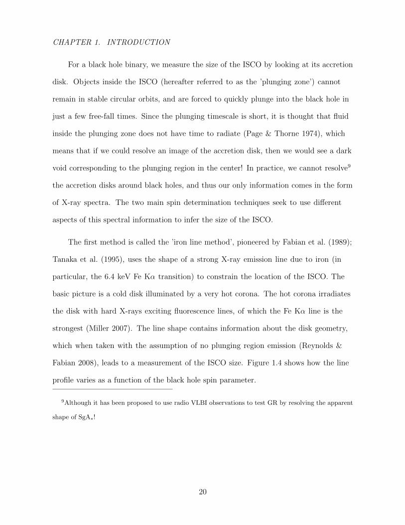
The first method is called the ’iron line method’, pioneered by Fabian et al. (1989);
Tanaka et al. (1995), uses the shape of a strong X-ray emission line due to iron (in
particular, the 6.4 keV Fe Kα transition) to constrain the location of the ISCO. The
basic picture is a cold disk illuminated by a very hot corona. The hot corona irradiates
the disk with hard X-rays exciting fluorescence lines, of which the Fe Kα line is the
strongest (Miller 2007). The line shape contains information about the disk geometry,
which when taken with the assumption of no plunging region emission (Reynolds &
Fabian 2008), leads to a measurement of the ISCO size. Figure 1.4 shows how the line
profile varies as a function of the black hole spin parameter.
9Although it has been proposed to use radio VLBI observations to test GR by resolving the apparent
shape of SgA∗!
20

CHAPTER 1. INTRODUCTION
θo = 40
ǫ= 3.0
−1.0
−0.5
−0.3
+0.0
+0.3
+0.6
+0.8
+1.0a
76.565.55
1.11.00.90.8
4
2
0
Energy [keV]
E/EeFlux[a.u.]
Figure 1.4: Iron line profiles for various choices of the black hole spin parameter a for a
disk viewed at 40o inclination. Here, the emissivity profile of the disk was set obeying the
power law F ∝ r−3. Notice that as the black hole spins up, the ISCO shrinks, resulting
in a stronger red-wing to the line profile. (Figure credit: Dauser et al. 2010)
This line modeling is complicated since the precise shape of the observed line profile
depends on four physical processes: 1) the emissivity profile for Fe Kα line as a function
of disk radius (which depends on both the degree of disk ionization and how the corona
irradiates the disk), 2) light-bending changing the apparent sizes of emitting regions, 3)
doppler boosting of the line, and 4) gravitational redshifting. The key piece of physics
used to infer the size of the ISCO is 4) – the gravitational redshifting produces a long red
tail in the line profile which cannot be due to processes 1-3. The maximum extent of this
red tail is set by fluorescing fluid that feels the strongest gravitational redshift (i.e. the
fluid right at the ISCO since the plunging region is assumed to be dark). This allows one
to determine the location of the ISCO (and hence the spin) from purely the line profile.
21
CHAPTER 1. INTRODUCTION
The second method (called the ’continuum fitting method’) uses the spectral shape
of the thermal continuum emission in the accretion disk to constrain the size of the ISCO
(originally applied by Zhang et al. 1997a with further refinements by Li et al. 2005;
Davis & Hubeny 2006; see table 2.3 for results from recent work). The idea of continuum
fitting is analogous to the operation in stellar astrophysics where one determines the
size of a star given only the spectrum. Given the temperature (which one gets from
the emission peak frequency), distance and flux, one can determine the star’s emitting
area (and hence size) without actually needing to resolve the star. For the purpose of
BH spin measurements, we determine the size of the accretion disk’s inner dark region
(the size of the ISCO) by observing the disk’s thermal spectra. The main drawback of
the continuum fitting method is that for it to work, we first need accurate estimates of
the BH distance (to turn fluxes into areas), disk inclination (to turn the area into an
ISCO radius), and BH mass (to get spin from the ISCO radius via figure 1.2). Luckily,
the techniques needed for measuring distance (Reid et al. 2011), mass, and inclination
(Cantrell et al. 2010; Orosz et al. 2011a,b) for binary systems are well known, and to
date have been successfully applied to about ten black hole binary systems (McClintock
et al. 2011). In table 1.1 below, we list a few recent measurements of black hole spins as
derived from the continuum fitting method.
1.3.2 Zoology of Disk States
In all previous discussions, we ignored the fact that the process of accretion is a time
dependent phenomenon. However, long term observations of black hole binary systems
reveal a rich variety of different accretion phases that each source cycles through.
22
CHAPTER 1. INTRODUCTION
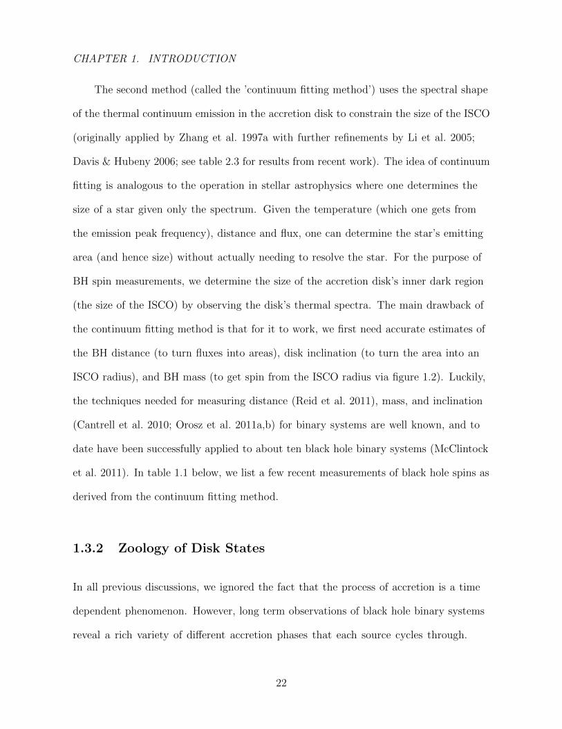
Figure 1.5 shows a few example spectra and power density spectra associated with the 3
primary states that stellar-mass black holes are observed to fall under (see McClintock &
Remillard 2006; Remillard & McClintock 2006b for an in-depth primer). Quantitatively,
four parameters are used to distinguish between the states, as listed below:
• the disk fraction f , which is the ratio of the thermal disk flux to the total (both
unabsorbed) over the 2-20keV band
• the power law index Γ of the high energy component of the flux
• the fractional Root-Mean-Squared (RMS) power r in the power density spectrum
integrated from 0.1-10Hz compared to the average source count rate
• the integrated RMS power qmax of any detected quasi-periodic-oscillation (QPO)
feature that is seen in the power density spectrum
The “thermal” state is characterized by strong continuum emission in the low energy
bands that is attributed to heat radiation from an optically thick accretion disk. The
overall fluctuations in the flux have a low RMS and are featureless, indicating a steady
accretion flow. There is also usually a weak high energy power law tail in the 2-20keV
band.
23

CHAPTER 1. INTRODUCTION
Figure 1.5: Examples of the three spectral states for black hole binaries. Absorption
corrected Spectral Energy Distributions (SED) are shown in the left panels, and their
corresponding power density spectra are shown on the right. The SEDs are decomposed
with a three component fit: thermal emission (red, solid), power-law (blue, dashed),
and relativistically broadened Fe Kα line (black, dotted). Figure Credit: Remillard &
McClintock 2006b
24
CHAPTER 1. INTRODUCTION
Strong power law emission with slope Γ ∼ 1.7 in the hard X-ray bands characterizes
the “hard” state of black hole binaries. Here, the fluctuations in the power spectrum are
significant (r > 0.1), and the prevailing picture is a hot accretion flow with negligible
thermal disk (Yuan & Narayan 2014). The hard state is also associated with the presence
of a quasi-steady radio jet, which produces strong correlations between X-ray and radio
flux of the system.
We also have the “steep power law” state, which shares many similarities to the
thermal state, but with a much stronger power law component and a steeper photon
index Γ ∼ 2.5. The differences between SPL and thermal are a fainter thermal disk
component in the former (SPL typical values f 50%), and a less variable but higher
sloped photon index in the latter. Perhaps the most exciting feature is the frequent
detection of strong QPOs in the SPL state. Typically, systems are found in the SPL
state when the luminosity approaches Eddington.
Finally, there is the quiescent state corresponding to extremely faint luminosities
(typically, more than 3 orders of magnitude fainter than the other states), where the
spectrum is nonthermal. The quiescent state is important since it allows for robust mass
determinations for these binary systems. The low disk luminosities allow the emission
from the secondary star to become prominent, which leads to accurate radial velocity
measurements.
25
CHAPTER 1. INTRODUCTION
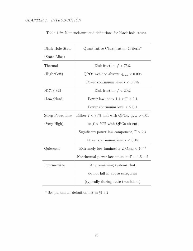
Table 1.2:: Nomenclature and definitions for black hole states.
Black Hole State: Quantitative Classification Criteriaa
(State Alias)
Thermal Disk fraction f > 75%
(High/Soft) QPOs weak or absent: qmax < 0.005
Power continuum level r < 0.075
H1743-322 Disk fraction f < 20%
(Low/Hard) Power law index 1.4 < Γ < 2.1
Power continuum level r > 0.1
Steep Power Law Either f < 80% and with QPOs: qmax > 0.01
(Very High) or f < 50% with QPOs absent
Significant power law component, Γ > 2.4
Power continuum level r < 0.15
Quiescent Extremely low luminosity L/LEdd < 10−3
Nonthermal power law emission Γ ∼ 1.5− 2
Intermediate Any remaining systems that
do not fall in above categories
(typically during state transitions)
a See parameter definition list in §1.3.2
26

CHAPTER 1. INTRODUCTION
Table 1.2 summarizes all the states of accretion in black hole binary systems. The
thermal state (associated with a steady accretion flow) is the only one that is well
understood from a theoretical standpoint (see the next section §1.4 for an overview of
the classic picture of disk physics). The complex time variability and multi-component
nature of the other states have made them difficult to analyze, motivating the need for
better accretion disk models. An active area of research is the study of the disk corona,
which is thought to be responsible for the power law emission at high energies. Open
questions remain about the corona’s geometry, strength, and generating mechanism that
we hope will be elucidated through better numerical modeling of the disk and beyond
(i.e. jets, winds, and corona).
1.4 Disk physics
Since a black hole does not radiate10, our only source of information comes from its
interaction on observable background/companion objects. In particular, the case of a
nearby massive companion star reaching the end of its life turns out to be the ideal
environment for detecting black holes. The star releases strong winds, overflows its
Roche lobe, and undergoes mass transfer onto the black hole.
This gradual inspiraling of material donated by the companion star forms an
accretion disk around the black hole. The disk has a few key properties that make
it useful for probing black hole physics: 1) it radiates incredibly brightly due to the
high temperatures induced by viscous processes in the disk making it easy to detect
10Ignoring Hawking radiation since its emission rate is negligible for astrophysical black holes
27
CHAPTER 1. INTRODUCTION
observationally; and 2) it reaches deep in the gravitational potential of the black hole,
with an inner edge at rms as discussed in §1.2.5 and thererby probing the multitude of
relativistic effects active in this region (frame dragging, doppler boosting, gravitational
redshifting, light bending, etc). Thus, an understanding of the accretion process is vitally
important if one wishes to connect black hole theory with observations.
1.4.1 Classic Thin Disk Model
It has been more than four decades since the landmark work of Shakura & Sunyaev
(1973) was published, giving birth to the whole subfield of accretion disk physics. Since
then many refinements have been made to the models, becoming ever more accurate and
precise (e.g. Pringle & Rees 1972; Lynden-Bell & Pringle 1974; Novikov & Thorne 1973;
Page & Thorne 1974; Pringle 1981, also see frank2002, kato08 for a thorough primer).
The standard assumptions made for modeling the accretion disk are:
• The disk is stationary and axisymmetric
• The disk is geometrically thin (h/r 1)
• Disk self gravity is negligible compared to that of the black hole
• No magnetic fields
• Radial and vertical structures can be decoupled
Given these simplifications, the goal is to solve for both the radial and vertical
structure of the disk obeying the usual physical constraints for gaseous astrophysical
systems. For a specific black hole configuration (i.e. black hole mass M , spin a, and
28
CHAPTER 1. INTRODUCTION
accretion rate M), as well as for a particular location in accretion disk r > rms, the game
is to simultaneously solve a system of equations that govern the physics of accretion. For
simplicity and to close the set of equations, one can simply assume a crude “one-zone”
model for the vertical structure and solve for the radial dependence of all disk quantities.
As we will see later, due to the polynomial nature of the various physics equations that
set the system, the final solution simplifies and takes the form of a series of power-law
scalings for each of the physical quantities.
Radial Structure
Amazingly, it is possible to deduce the radial energetics of the system with only very
few assumptions. Although viscous angular momentum transport ultimately governs the
diffusion of material within the accretion disk, a precise understanding of viscosity within
the disk is not needed provided that the resultant radial transport of material is slow
(i.e. whenever the viscous radial advection timescale greatly exceeds the vertical thermal
diffusivity timescale). Under this assumption, the flux of energy out of the disk does not
depend on the precise nature of viscosity – it is simply the rate at which gravitational
potential energy is dissipated and released via local radiative cooling of the accreting
matter.
We illustrate the exercise in the Newtonian limit for simplicity. Given a disk with
mass accretion rate M and assuming the gas follows Keplerian circular orbits with
orbital frequency ΩK =√GM/r3, the system of equations that must be solved to yield
29

CHAPTER 1. INTRODUCTION
the energy flux is simply:
dM
dr= 0, (conservation of mass) (1.33)
Md (ΩKr
2)
dr=d (2πr2W )
dr. (— of angular momentum) (1.34)
F =d(3ΩKW )
dr, (— of energy) (1.35)
where W represents the vertically integrated shear stress trφ of the disk
W (r) =
∫trφ(r, z)dz. (1.36)
Solving Eqs. 1.33-1.36 for F yields the classic disk solution:
F (r) =3GMM
8πr3
(1−
√r
rin
), (1.37)
where the constant of integration is set by rin = rms, corresponding to the innermost
radius of the disk where the flux vanishes.
Vertical Structure
Now, armed with the radial flux profile, one can solve for various other physical quantities
that relate to the vertical structure of the disk. The usual approach is to introduce height
integrated quantities to collapse the vertical structure, making the system of equations
tractable algebraically (e.g. defining a vertically integrated column density Σ ≡ 2Hρ,
where H is some characteristic height of the disk and ρ is the central gas density). The
key equations relating to vertical structure are:
dPtot
dz= −ρgz, (hydrostatic balance) (1.38)
F = −4acT 3
3κρ
∂T
∂z, (radiative flux) (1.39)
M = −2πr
∫vrρdz (mass accretion), (1.40)
30
CHAPTER 1. INTRODUCTION
where Ptot = Pgas + Prad is the total pressure, gz ∼ ΩKH is the vertical disk gravity, T
is the disk temperature, κ is the opacity law (typically a combination of free-free and
electron scattering), and vr is the characteristic radial advection velocity of the gas.
Closure Equations
A few more equations are needed to close the system of equations and yield a complete
disk solution:
Equation of State : Ptot(ρ, T ) (1.41)
Opacity Law : κ(ρ, T ) (1.42)
α-Prescription for Stress : trφ = αPtot (1.43)
The last closure relation with a constant α is simply an ansatz that was originally
motivated by a combination of dimensional analysis and algebraic convenience. Luckily,
it has been borne out by recent investigations of computer simulations of turbulence
(Stone et al. 2008; Hirose, Blaes & Krolik 2009; Hirose, Krolik & Blaes 2009; Jiang
et al. 2012, 2013). It appears to hold remarkably well for a whole host of accretion disk
simulation parameters, with α ∼ 0.01− 0.1 depending on the details of simulations.
Finally, combining all the vertically integrated forms of the physics equations along
with the three closure relations results allows one to solve for all relevant accretion disk
quantities. For the sake of brevity, we only list below the relativistic solution worked out
by Novikov & Thorne (1973) for the disk properties and Page & Thorne (1974) for the
flux profile. Please refer to Shakura & Sunyaev (1973) for Newtonian disk solutions.
31
CHAPTER 1. INTRODUCTION
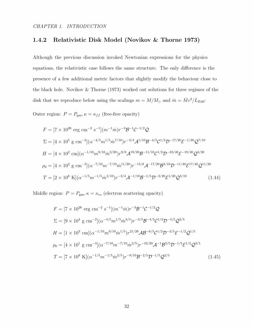
1.4.2 Relativistic Disk Model (Novikov & Thorne 1973)
Although the previous discussion invoked Newtonian expressions for the physics
equations, the relativistic case follows the same structure. The only difference is the
presence of a few additional metric factors that slightly modify the behaviour close to
the black hole. Novikov & Thorne (1973) worked out solutions for three regimes of the
disk that we reproduce below using the scalings m = M/M and m = Mc2/LEdd:
Outer region: P = Pgas, κ = κff (free-free opacity)
F = [7× 1026 erg cm−2 s−1](m−1m)r−3B−1C−1/2Q
Σ = [4× 10⁵ g cm−2](α−4/5m1/5m7/10)r−3/4A1/10B−4/5C1/2D−17/20E−1/20Q7/10
H = [4× 102 cm](α−1/10m9/10m3/20)r9/8A19/20B−11/10C1/2D−23/40E−19/40Q3/20
ρ0 = [4× 10² g cm−3](α−7/10m−7/10m11/20)r−15/8A−17/20B3/10D−11/40E17/40Q11/20
T = [2× 10⁸ K](α−1/5m−1/5m3/10)r−3/4A−1/10B−1/5D−3/20E1/20Q3/10 (1.44)
Middle region: P = Pgas, κ = κes (electron scattering opacity)
F = [7× 1026 erg cm−2 s−1](m−1m)r−3B−1C−1/2Q
Σ = [9× 10⁴ g cm−2](α−4/5m1/5m3/5)r−3/5B−4/5C1/2D−4/5Q3/5
H = [1× 103 cm](α−1/10m9/10m1/5)r21/20AB−6/5C1/2D−3/5E−1/2Q1/5
ρ0 = [4× 101 g cm−3](α−7/10m−7/10m2/5)r−33/20A−1B3/5D−1/5E1/2Q2/5
T = [7× 10⁸ K](α−1/5m−1/5m2/5)r−9/10B−2/5D−1/5Q2/5 (1.45)
32

CHAPTER 1. INTRODUCTION
Inner region: P = Prad, κ = κes
F = [7× 1026 erg cm−2 s−1](m−1m)r−3B−1C−1/2Q
Σ = [5 g cm−2](α−1m−1)r3/2A−2B3C1/2EQ−1
H = [1× 105 cm](m)A2B−3C1/2D−1E−1Q
ρ0 = [2× 10⁻⁵ g cm−3](α−1m−1m−2)r3/2A−4B6DE2Q−2
T = [5× 10⁷ K](α−1/4m−1/4)r−3/8A−1/2B1/2E1/4 (1.46)
where the radial functions are defined as: (in terms of dimensionless radius x =√r/M
and dimensionless spin a∗ = a/M):
A = 1 + a2∗x−4 + 2a2
∗x−6
B = 1 + a∗x−3
C = 1− 3x−2 + 2a∗x−3
D = 1− 2x−2 + a2∗x−4
E = 1 + 4a2∗x−4 − 4a2
∗x−6 + 3a4
∗x−8
Q =1 + a∗x
−3
x(1− 3x−2 + 2a∗x−3)1/2
[x− x0 −
3
2a∗ ln
(x
x0
)− 3(x1 − a∗)2
x1(x1 − x2)(x1 − x3)ln
(x− x1
x0 − x1
)3(x2 − a∗)2
x2(x2 − x1)(x2 − x3)ln
(x− x2
x0 − x2
)− 3(x3 − a8)2
x3(x3 − x1)(x3 − x2)ln
(x− x3
x0 − x3
)](1.47)
where the cofactors are set by:
x0 =√rms/M
x1 = 2 cos[(cos−1 a∗ − π)/3
]x2 = 2 cos
[(cos−1 a∗ + π)/3
]x3 = −2 cos
[(cos−1 a∗)/3
](1.48)
33
CHAPTER 1. INTRODUCTION
Due to its prevalence in the black hole accretion disk literature, we will make extensive
use of this model in the remaining chapters of this thesis.
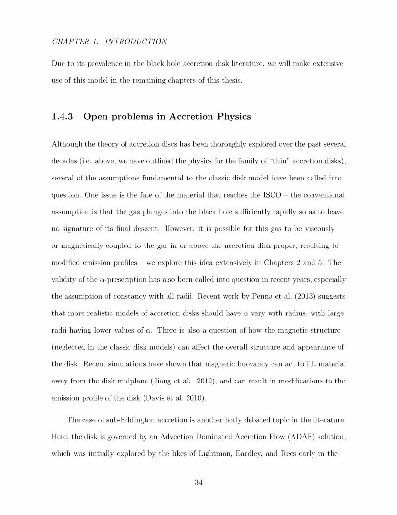
1.4.3 Open problems in Accretion Physics
Although the theory of accretion discs has been thoroughly explored over the past several
decades (i.e. above, we have outlined the physics for the family of “thin” accretion disks),
several of the assumptions fundamental to the classic disk model have been called into
question. One issue is the fate of the material that reaches the ISCO – the conventional
assumption is that the gas plunges into the black hole sufficiently rapidly so as to leave
no signature of its final descent. However, it is possible for this gas to be viscously
or magnetically coupled to the gas in or above the accretion disk proper, resulting to
modified emission profiles – we explore this idea extensively in Chapters 2 and 5. The
validity of the α-prescription has also been called into question in recent years, especially
the assumption of constancy with all radii. Recent work by Penna et al. (2013) suggests
that more realistic models of accretion disks should have α vary with radius, with large
radii having lower values of α. There is also a question of how the magnetic structure
(neglected in the classic disk models) can affect the overall structure and appearance of
the disk. Recent simulations have shown that magnetic buoyancy can act to lift material
away from the disk midplane (Jiang et al. 2012), and can result in modifications to the
emission profile of the disk (Davis et al. 2010).
The case of sub-Eddington accretion is another hotly debated topic in the literature.
Here, the disk is governed by an Advection Dominated Accretion Flow (ADAF) solution,
which was initially explored by the likes of Lightman, Eardley, and Rees early in the
34
CHAPTER 1. INTRODUCTION
1970’s. Interest in this topic was later revived in the 1990’s (Narayan & Yi 1994;
Abramowicz et al. 1995). In recent years, various groups have proposed different
mechanisms that can achieve the radiatively inefficient property of the ADAF such
as the advection dominated inflow-outflow solution (ADIOS – Blandford & Begelman
1999) or the convection dominated accretion flow (CDAF – Narayan, Igumenshchev
& Abramowicz 2000), which has led to an ongoing debate as to which of the models
is the most physically realistic. It is also an open question (both observationally and
theoretically) as to how these systems transition from the standard thin accretion disk
state to the ADAF state – the current state of affairs is described in Yuan & Narayan
2014.11
Perhaps the least understood aspect of disk models relates to the case of super-
Eddington accretion, where the radiative output of the disk can become so extreme
as to limit/halt the supply of infalling matter. This phase of accretion is crucial for
understanding the AGN population and the quasar luminosity function since it acts
as a limiter on black hole growth. Recent observations of supermassive quasars at
high redshift (e.g. 1.2 × 10¹⁰M at redshift z = 6.3; Wu et al. 2015) suggest that the
Eddington limit can be broken (otherwise, how could such massive black holes exist at
such early times?). This is also borne out in recent numerical simulations of accreting
black holes (Sadowski & Narayan 2015b) suggests that the apparent luminosity can reach
as high as thousands of Eddington units. However, there is no consensus yet on how far
the Eddington limit can be exceeded and is currently an area of active research.
11One idea (posited by Narayan and collaborators) is that at low accretion rates, say m ∼ 0.01, the
innermost parts of the usual thin accretion disk puff up into the ADAF state, with a transition radius
being set according to m
35

CHAPTER 1. INTRODUCTION
Finally, there is a question of how jets are formed, and where the energy that
powers the jet is being extracted from. One idea that is that the black hole rotational
energy could be tapped to power a jet. The Blandford & Znajek (1977) mechanism is
the leading model for explaining how jets can be launched as a consequence of a black
hole’s spin interaction with its embedded magnetic field. This jet formation mechanism
has been verified in numerical simulations of accretion (Tchekhovskoy et al. 2011;
Tchekhovskoy & McKinney 2012). Alternative ideas include magnetically driven winds
in the disk collimating to become a jet (Blandford & Payne 1982), or radiatively driven
jets (Sadowski & Narayan 2015b).
Ultimately, due to the complexity and nonlinearity of the physics involved (i.e.
electromagnetism, relativity, radiative transport, fluid-dynamics, turbulence), computer
simulations give perhaps the best shot at understanding the true nature of the accretion
process.
1.5 Numerical Simulations
The physics of accretion is a messy business; the precise details are the result of the
interplay between the physics of general relativity (due to proximity to a compact
object), hydrodynamics (since the accretion flow is a gaseous fluid), magnetism (the
magneto-rotational instability is the chief driver of turbulence, and hence viscosity), and
radiation (how we ultimately observe the disks). Finally there is the issue of accretion
disks being multidimensional objects, coupled with the fact that disk MHD turbulence
has to be studied in three dimensions with high resolving power. All this contributes to
a significant computational expense. Another factor adding to the difficulty is the large
36
CHAPTER 1. INTRODUCTION
range of dynamical scales in the problem – although most of the action and energetics
are concentrated close to the black hole with a rather short characteristic timescale, the
gas in the disk flows in from much farther out, evolving on a much long viscous time at
large radii. Due to these challenges, it is only within the last decade that it has been
possible to tackle this difficult problem computationally (and even still, most current
codes only consider a subset of the physics!).
To date, there are a wide variety of relativistic hydrodynamic codes available. A
partial list includes: ATHENA (Stone et al. 2008), Cosmos++ (Anninos et al. 2005),
ECHO (Del Zanna et al. 2007), HARM (Gammie et al. 2003), HERACLES (Gonzales,
Audit, & Huynh 2007), KORAL (Sadowski et al. 2013), RAISHIN (Mizuno et al. 2006),
ZEUS (Hayes & Norman 2003) etc... Typically, the codes fall into one of two categories:
1) local shearing box simulations, which are designed to focus on resolving the onset of
the turbulent dynamo at small scales, or 2) global simulations that seek to capture the
full three-dimensional structure and evolution of disk material.
The approach taken for handling fluid dynamics also spans multiple paradigms.
The most common approaches include artificial viscosity schemes (Wilson 1972), and
Godunov-type methods that make use of approximate or exact Riemann solvers. In
either case, finite difference representations are used for handling the general relativistic
hydrodynamic equations. The advantage of the artificial viscosity technique is that it is
more straightforward to implement, can be easily extended to include additional physics,
and is less expensive than Godunov schemes. However, Godunov schemes enjoy the
distinction of being fully conservative by design (and thus potentially more accurate) even
in the case of ultrarelativistic flows. They also require less tuning since a viscosity term
does not have to be set. However the tradeoff is that the system then becomes subject
37
CHAPTER 1. INTRODUCTION
to numerical viscosity, which depends sensitively on the simulation setup (i.e. spatial
grid resolution and accuracy of the Riemann solver). Aside from these two primary
approaches, other schemes include smooth-particle hydrodynamics(Lucy 1977; Gingold
& Monaghan 1977; Springel, Yoshida & White 2001) and spectral methods(Canuto et al.
1988), though they are less well-developed in the field of relativistic accretion.
1.5.1 Shearing Boxes
For the problem of simulating numerical accretion disks, a decision must be made as
to whether the problem should be tackled piecewise locally, or in a global sense. The
former case lends itself to “shearing box” simulations, where the accretion flow is studied
in detail locally and mimics the shear present in a small rectangular patch of disk. All
disk structure is handled via appropriate choice of boundary conditions, ignoring the
remaining large scale structure of the disk. The most obvious advantage of this approach
is that by focusing only on a small patch, high spatial resolutions can be achieved,
allowing the turbulent process to be completely resolved.
Perhaps the most significant breakthough resulting from shearing-box simulations
has been the discovery and exploration of the magneto-rotational instability (MRI) in
accretion disks (Balbus & Hawley 1991, 1998). This instability is able to amplify any
poloidal seed magnetic field, growing the field strength exponentially until it reaches a
nonlinear turbulent saturation state. It resolved a longstanding problem in accretion
disk theory, explaining the mechanism for the turbulent fluctuations that give rise to
the viscous transport of material in discs. Prior to the MRI, all other mechanisms (e.g.
convection, gas-dynamical viscosity) were found to be far too weak to account for the
38

CHAPTER 1. INTRODUCTION
observed properties of accretion disks. Generally, shearing box simulations reproduce
viscosity laws that resemble the α-prescription as mentioned in §1.4.1, with typical
values α ∼ 0.05 (Blackman et al. 2008; Guan et al. 2009; Hawley et al 2011; Sorathia
et al. 2012) although it has been found to depend weakly on the net initial magnetic
field (Hawley et al. 1995; Pessah et al. 2007) and also the numerical setup/resolution
(Fromang & Papaloizou 2007; Davis et al. 2010; Bai & Stone 2013).
Recently, shearing boxes have been useful for investigating properties of radiatively
dominated discs. By including a radiation scheme known as Flux Limited Diffusion
(FLD), Turner and Hirose were able to study the evolution of vertical structure within
accretion disks. However recently, tension has mounted among different groups for the
topic of disk stability in the radiation dominated limit (Jiang vs Hirose).
1.5.2 Global Simulations
Simulating the accretion problem globally is a far more computationally taxing problem
due to the huge range of dynamical scales involved. Compared to shearing-box
simulations, sacrifices must be made for the sake of computational expediency, such as
much lower spatial resolutions, dropping some of the physics (e.g. ignoring radiation), or
reducing dimensionality. However, global simulations are necessary since they are the
only method that can capture the full effects of relativity on the accretion disk as well
as connecting the turbulent evolution of the magnetic field with properties of the disk at
large.
The earliest works for simulating accretion discs in a global sense were that of
Wilson, who pioneered the field when he numerically considered the hydrodynamical
39
CHAPTER 1. INTRODUCTION
problem of spherical accretion of material with non-zero angular momentum. Wilson
found that the centrifugal barrier induced by the material’s angular momentum led to the
formation of a fat non-accreting torus. Interest in the field of numerical global accretion
has grown over time due to the recent trend of exponential growth in computational
power. The last decade has seen the rise of a wide variety of magneto-hydrodynamic
(MHD) codes tailored for the problem of accretion. The focus on MHD is well-motivated
since magnetic fields play such a pivotal role in accretion – acting as both a generator
for the turbulent motions (via MRI) and as a mechanism for launching and confining
jets (Blandford-Znajek).
This has spurred a decade of furious activity in the field, with early work carried
out in nonrelativsitic frameworks although taking advantage of a pseudo-Newtonian
potential to simulate some of the relativistic effects (Armitage 1998; Hawley & Krolik
2001; Igumenshchev et al. 2003). General-relativistic formulations of these simulations
were developed soon after (Koide et al 1999; De Villiers & Hawley 2003; Gammie et al.
2003; Fragile et al. 2007) and most of the recent discoveries on disk/jet physics are based
on these codes.
1.5.3 Future Directions
To date, most numerical simulations of accretion have either ignored radiation altogether
or have implemented extremely crude/unrealistic models of the radiation. This is a
deliberate choice and reflects the difficulty of the physics involved. Since the radiation
field is a seven dimensional quantity12, it is quite complex to model and poses a huge
12Radiation involves three spatial, two angular, one time, and one frequency dimension
40
CHAPTER 1. INTRODUCTION
challenge in terms of computational resources (see §1.6 for more details). It is only in the
past few years that radiatively coupled MHD simulations have become feasible, initially
without including relativity (Ohsuga et al. 2009; Ohsuga & Mineshige 2011; Jiang, Stone
& Davis 2014). The current push in the numerical accretion community is to tackle the
full GRMHD and radiation problem (Sadowski et al. 2013; McKinney et al. 2014).
1.6 Including Radiation
So far, we have seen a decade of success in the realm of general relativistic magneto
hydrodynamic (GRMHD) codes (Gammie et al. 2003; DeVilliers & Hawley 2003; Shafee
et al. 2008; Noble et al. 2009; Penna et al. 2010; McKinney et al. 2012; Narayan et al.
2012). However, as already mentioned, radiation has typically been neglected for the
sake of computational speed. Although there are several prior examples of radiation
hydrodynamic codes in the literature, none were capable of handling the full general
relativistic problem in three-dimensions. Nevertheless, due to the exponential growth of
computing power in recent times, we are now poised to tackle this problem in full-force
(i.e. including radiation). Presently, radiation hydrodynamics is an active area of
research being pursued by several accretion disk research groups (and our group is no
exception!); it is the final unexplored frontier in numerical accretion.
Generally, codes that model radiation fall under four broad categories, distinguished
by their radiative transport algorithms. These four numerical treatments of radiation
transport are:
• Diffusion – Radiation is treated as simply another independent relativistic fluid.
41
CHAPTER 1. INTRODUCTION
The radiation energy density is the key parameter that dictates its flow and
transport.
• Discrete Ordinates – The radiation field is interpreted as a finite collection of
rectilinear light rays (i.e. light is modeled to travel along a finite set of angles).
• Spherical Harmonics – Decompose the radiation field into various spherical
harmonic moments. These moments can then be easily evolved in time
independently as the propagation of spherical waves.
• Monte Carlo – Introduce and track a large number of individual simulated photons.
1.6.1 Radiation Hydrodynamics
Historically, radiation hydrodynamics has been successfully applied in several other
astrophysical contexts, such as the cores of collapsing supermassive stars (to understand
the ignition mechanism for supernovae – Nordhaus et al 2010), star formation within the
ISM (Haworth & Harries 2012), and models of the solar corona (e.g. flares – Fisher 1986).
However, the added complexity and computational cost of marrying radiation, fluid
mechanics, and general relativity has resulted in a paucity of codes capable of tackling
the problem of BH accretion. To date, there are only a handful of groups concurrently
developing codes to handle radiative hydrodynamics, either in a local shearing box
(Hirose, Blaes & Krolik 2009; Jiang et al. 2012), or in a global fully realized accretion
disk (Farris et al. 2008; Ohsuga & Mineshige 2011; Fragile et al. 2012).
42

CHAPTER 1. INTRODUCTION
Figure 1.6: The radiation temperature distribution in the ‘hohlraum’ problem (radiation
leaking into a cavity with a central rectangular block) as computed by Brunner (2002).
The panels represent results calculated via the four paradigms: a)Diffusion, b)Discrete
Ordinates, c)Spherical Harmonics, and d)Monte Carlo.
For the purposes of relativistic hydrodynamics, the radiative diffusion model is
the natural choice as it is in essence a fluid treatment of radiation (making it easy to
merge with the fluid treatment of gas). Additionally, the other methods suffer from
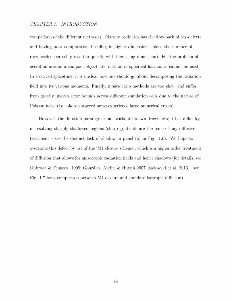
various defects that make them unattractive for our purposes (see Fig. 1.6 for a visual
43
CHAPTER 1. INTRODUCTION
comparison of the different methods). Discrete ordinates has the drawback of ray-defects
and having poor computational scaling in higher dimensions (since the number of
rays needed per cell grows too quickly with increasing dimension). For the problem of
accretion around a compact object, the method of spherical harmonics cannot be used;
In a curved spacetime, it is unclear how one should go about decomposing the radiation
field into its various moments. Finally, monte carlo methods are too slow, and suffer
from greatly uneven error bounds across different simulation cells due to the nature of
Poisson noise (i.e. photon starved areas experience large numerical errors).
However, the diffusion paradigm is not without its own drawbacks; it has difficulty
in resolving sharply shadowed regions (sharp gradients are the bane of any diffusive
treatment – see the distinct lack of shadow in panel (a) in Fig. 1.6). We hope to
overcome this defect by use of the ‘M1 closure scheme’, which is a higher order treatment
of diffusion that allows for anisotropic radiation fields and hence shadows (for details, see
Dubroca & Feugeas 1999; Gonzales, Audit, & Huynh 2007; Sadowski et al. 2013 – see
Fig. 1.7 for a comparison between M1 closure and standard isotropic diffusion).
44

CHAPTER 1. INTRODUCTION
Figure 1.7: The radiation temperature distribution in a shadowing test, where highly
beamed light shines on an optically thick sphere. Panel a) is the result from the simple
diffusive treatment of radiation, whereas b) is the result from M1 closure (as calculated by
Gonzales, Audit, & Huynh 2007). Notice that the M1 closure scheme is able to accurately
handle shadowing, despite being a diffusive treatment. Panel c) shows the results from
Sadowski et al. (2013), also using M1.
1.7 Chapter Summaries
Chapter 2 compares spectral calculations of GRMHD accretion disks from (Penna et al.
2010) to those of the classic (Novikov & Thorne 1973) disk models. The GRMHD disk
simulations capture all but the radiation physics for magnetized flow around a black
45
CHAPTER 1. INTRODUCTION
hole. We apply radiative transfer post-processing to get simulated images of the discs
making use of the 1D radiative transfer solutions of TLUSTY (Hubeny & Lanz 1995).
This is an advance over previous work on computing GRMHD disk spectra (Kulkarni
et al. 2011), which only assumed (modified) blackbody annuli spectra. The following are
the key results from our investigation:
(1). The GRMHD based accretion discs have hotter spectra than the standard Novikov
& Thorne (1973) discs. The GRMHD discs produce more luminosity everywhere,
and the contrast becomes most apparent inside the ISCO.
(2). The increased luminosity of the GRMHD discs compared to the classic NT discs
induces a modest systematic bias in the derived spins of these GRMHD discs. For
black holes of spin a∗ = 0, 0.7, 0.9 the spin deviation is ∆a∗ ∼ 0.15, 0.07, 0.03 in
the worst cases (corresponding to inclination angles of 75).
(3). The GRMHD discs around spinning black holes exhibit a weak high-energy
power-law tail. This power-law tail arises from the combined emission of the hot
plunging region gas. The strength of this plunging region power-law increases with
the system’s inclination angle.
In Chapter 3, we develop a simple one-zone model for black hole accretion discs that
include both convective and turbulent vertical energy transport channels. We find that
the action of mixing from convection and turbulence provides a stabilizing effect on the
46
CHAPTER 1. INTRODUCTION
disk, pushing the threshold for thermal instability up towards higher accretion rates. In
some cases, we find that turbulent mixing pushes the threshold for instability far above
10 per cent Eddington – even inducing complete stability in the most extreme cases.
This is in agreement with previous studies that show convective mixing protects against
the onset of thermal instability. However since MRI-induced turbulence is much more
vigorous than convective turbulence, it is not surprising that turbulently mixed discs
experience a much stronger version of this stabilizing effect.
Chapter 4 describes HERO, a new general relativistic radiative transfer code. It is
primarily designed to model the radiation field for accretion flows around black holes.
The unique features of HERO are: 1) it uses a hybrid short/long characteristics radiative
solver; and 2) it is implemented in a general relativistic framework that takes into
account the effects of light bending, doppler beaming, and gravitational redshifting.
HERO is written as a post-processing code decoupled from the hydrodynamic evolution
of the fluid. It computes the time-independent radiation field assuming a given fixed
background fluid structure. To verify that HERO produces physically correct answers, we
have performed a comprehensive set of tests designed to examine the code’s convergence
properties, accuracy, and capability to handle multidimensional relativistic problems. We
also confirm the well known result that 2D and 3D problems with compact sources suffer
from significant ray defects in the far field when analyzed with the short characteristics
method. We present an approximate fix which mitigates the effects in the case of a 3D
spherical grid. However, for accurate results, we find that it is necessary to switch to a
long characteristics solver which is unaffected by ray-defects.
Chapter 5 covers the Comptonization module that we develop for HERO.
Comptonization is handled through a quadratic Kompaneets based solver that
47

CHAPTER 1. INTRODUCTION
evolves light rays by means of a modified Comptonized source function. We test our
Comptonization module by comparing with exact solutions of light diffusing through
purely scattering media. We find excellent agreement between HERO and the exact
solutions for both 1D and 3D test problems. We also apply our code to the astrophysical
problem of radiation emerging from an accretion disk. The self consistent temperature
and radiation fields throughout the accretion disk are calculated taking into account
relativistic effects, returning disk radiation, and Compton cooling. The complete solution
results in a two-phase disk structure, with a hot spherical corona surrounding a cooler
thermal disk. Finally, performing raytracing on the solution yields integrated disk
spectra with slightly higher spectral hardening factors compared to previous 1D based
estimates. We also verify the Zhu et al. (2012) result of a high-energy power law tail
feature emerging in the spectrum of a black hole accretion disk.
48
Chapter 2
The Eye of the Storm:
Light from the Inner Plunging
Region of Black Hole Accretion Discs
This thesis chapter originally appeared in the literature as
Y. Zhu, S.W. Davis, R. Narayan, A.K. Kulkarni, R.F. Penna,
J. E. McClintock, MNRAS, 424, 250, 2012
Abstract
It is generally thought that the light coming from the inner plunging region of black hole
accretion discs contributes negligibly to the disc’s overall spectrum, i.e. the plunging
fluid is swallowed by the black hole before it has time to radiate. In the standard disc
49
CHAPTER 2. LIGHT FROM THE PLUNGING REGION OF ACCRETION DISCS
model used to fit X-ray observations of accretion discs, the plunging region is assumed
to be perfectly dark. However, numerical simulations that include the full physics of
the magnetized flow predict that a small fraction of the disc’s total luminosity emanates
from this plunging region. In this work, we investigate the observational consequences
of this neglected inner light. We compute radiative transfer based disc spectra that
correspond to 3D general relativistic magnetohydrodynamic simulated discs (which
produce light inside their plunging regions). In the context of black hole spin estimation,
we find that this neglected inner light only has a modest effect (this bias is less than
typical observational systematic errors). For rapidly spinning black holes, we find that
the combined emission from the plunging region produces a weak power-law tail at high
energies. This indicates that infalling matter is the origin for some of the ‘coronal’
emission observed in the thermal dominant and steep power-law states of X-ray binaries.
2.1 Introduction
The ubiquity and simplicity of black holes in our universe make them truly marvelous
objects of study. The complete physics of each and every black hole (BH) can be distilled
down to just two numbers1: the black hole’s mass M and angular momentum J , the
latter of which is usually expressed as a dimensionless spin parameter a∗ = J/(GM2/c).
This implies that all physical theories that involve black holes, e.g. the link between
BH spin and jet power (Blandford & Znajek 1977), Gamma Ray Bursts and spinning
BHs (MacFadyen & Woolsley 1999), models of quasi-periodic oscillations (Abramowicz
1In principle, BH charge is an independent parameter; however, we do not expect astrophysical black
holes to retain any significant charge.
50

CHAPTER 2. LIGHT FROM THE PLUNGING REGION OF ACCRETION DISCS
& Kluzniak 2001), must connect in some way to these two numbers.
For binary systems, the task of measuring mass is relatively straightforward; so
long as one can obtain the period, orbital velocity, orbital geometry (i.e. inclination
and eccentricity), and mass for a companion orbiting a black hole, one can immediately
obtain the black hole mass using only Newtonian gravity (for a recent example, see
Orosz et al. 2011b). The game of measuring black hole masses has been played as early
as 1972 for Cygnus X-1 (Webster & Murdin 1972; Bolton 1972), and to date we have
robust mass estimates for about 20 stellar mass binary black hole systems (Remillard
& McClintock 2006b; Orosz et al. 2007, 2009, 2011a,b; Cantrell et al. 2010), and ∼50
supermassive black holes (Gultekin et al. 2009).
Despite this success in measuring black hole mass, spin has been a more difficult
quantity to obtain. The spin of an object only makes itself known at very short distances
through a general relativistic effect known as frame dragging. Thus to probe black hole
spin, we must rely on observations of matter that is very close to the BH horizon. In
practice, the only available probe is the accretion disc orbiting the black hole, which
transitions from nearly circular orbits to plunging at a special location known as the
innermost stable circular orbit (ISCO). By observing the light given off by the accretion
disc, it is possible to determine this transition radius. When the ISCO is expressed in
terms of the gravitational radius rg = GM/c2, it has a well-defined monotonic dependence
on black hole spin (e.g. Shapiro & Teukolsky 1983). Therefore, a measurement of the
ISCO size yields the BH spin if the mass is independently known.
For a black hole binary system, we measure the size of the ISCO by modelling the
light given off by the accretion disc. Objects inside the ISCO (hereafter referred to as
51
CHAPTER 2. LIGHT FROM THE PLUNGING REGION OF ACCRETION DISCS
the ‘plunging zone’) cannot remain in stable circular orbits, and are forced to quickly
plunge into the black hole in just a few free-fall times. Since the plunging time-scale is
short, it is thought that fluid inside the plunging zone does not have time to radiate
(Page & Thorne 1974), which means that if we could resolve an image of the accretion
disc, then we would see a dark void corresponding to the plunging region in the centre.
In practice, we cannot resolve images2 of accretion discs around black holes, and thus
our only information comes in the form of X-ray spectra.
One method of estimating BH spin3 works by fitting the spectral shape of the
thermal continuum emission from the accretion disc to thereby estimate the radius of the
ISCO (this method was pioneered by Zhang et al. 1997a; see Table 2.3 for some recent
results).
This ‘continuum fitting’ method uses the colour temperature of the thermal
component, the distance to the source, and the received X-ray flux to obtain a
characteristic emitting area for the disc. Given a model for the radial dependence of the
disc emission, this characteristic emitting area determines the ISCO radius. The main
drawback of the continuum fitting method is that we first need accurate estimates of
the BH distance (to turn fluxes into areas), disc inclination (to turn the projected area
into an ISCO radius), and BH mass (to get spin from the monotonic rISCO/rg vs. a∗
relation). Luckily, the techniques needed for measuring distance (Reid et al. 2011), mass,
2Although it has been recently proposed to use radio VLBI observations to test GR by resolving the
apparent shape of SgrA∗ (Doeleman et al. 2009).
3Another commonly applied method is known as the ‘iron line’ method, which estimates BH spin
through spectral modelling of the Fe Kα fluorescence line (Fabian et al. 1989, see Miller 2007 for a recent
review).
52
CHAPTER 2. LIGHT FROM THE PLUNGING REGION OF ACCRETION DISCS
and inclination (Orosz et al. 2011b; Cantrell et al. 2010) for binary systems are well
developed, and to date have been successfully applied to more than half a dozen black
hole binary systems (McClintock et al. 2011).
The continuum fitting method has evolved through a sequence of progressively more
complex disc models. The simplest model assumes multitemperature blackbody emission
from the disc (Mitsuda et al. 1984). Including relativistic effects such as Doppler beaming,
gravitational redshifting, and light bending yielded the next generation of models (called
kerrbb – Li et al. 2005). The current generation of disc models (named bhspec –
Davis et al. 2005; Davis & Hubeny 2006) frees itself from the blackbody assumption, and
instead obtains the disc spectra by means of radiative transfer calculations. All of the
above mentioned models use the prescription of Novikov & Thorne (1973, hereafter NT)
as the underlying disc model4, which assumes a perfectly dark void inside the ISCO. The
advance that we make in this work is to apply radiative transfer calculations to compute
the spectrum for a general relativistic magneto-hydrodynamic (GRMHD) simulated disc
that produces emission from inside the ISCO.
4This is the relativistic generalization of the standard Shakura & Sunyaev (1973) model for viscous
geometrically thin but optically thick accretion discs.
53

CHAPTER 2. LIGHT FROM THE PLUNGING REGION OF ACCRETION DISCS
Figure 2.1: Comparison of dimensionless luminosity profiles from the GRMHD simu-
lations of Penna et. al 2011 (solid) with the standard disc model (dotted – Novikov &
Thorne 1973; Page & Thorne 1974). Results from models A,B,C (defined in Table 2.1),
are shown. The dashed line depicts an alternate measure of the GRMHD luminosity (de-
scribed in §2.7.2 and Appendix 2.12). Note that the luminosity in the standard Novikov
& Thorne (1973) disc model goes to zero at the ISCO.
Currently, a crucial assumption in the continuum fitting enterprise is the perfect
darkness of the plunging zone. This scenario applies only to the idealized case of a razor
thin unmagnetized disc (see Novikov & Thorne (1973)). For finite thickness discs, it
has been argued that as long as the disc remains geometrically thin (with disc aspect
ratios h/r 1), the disc can be well approximated by the NT model (Paczynski 2000;
54

CHAPTER 2. LIGHT FROM THE PLUNGING REGION OF ACCRETION DISCS
Afshordi & Paczynsky 2003; Shafee et al. 2008a). However, recent work with magnetized
discs (Shafee et al. 2008b; Noble et al. 2009, 2010, 2011; Penna et al. 2010) suggests
that there may be departures from NT even in the limit of thin discs. An observational
difference between these magnetized discs and the classic NT discs is the appearance
of non-negligible luminosity inside the plunging region (see Fig. 2.1 for the result from
Penna et al. (2010), where the extra plunging region luminosity constitutes ∼ 4 per cent
of the total). Recent models of unmagnetized discs that include the physics of energy
advection (Abramowicz et al. 1988; most recently Sadowski 2009, Sadowski et al. 2011)
also share the feature of nonzero luminosity inside the ISCO, but in these advective
models, the extra light only becomes significant when the accretion rate approaches the
Eddington rate.
The primary goal of the present project is to investigate the importance of the
neglected light from the inner plunging region of accretion discs. Since GRMHD discs
exhibit the phenomenon that we wish to investigate (i.e. nonzero light from the plunging
region), we use them as the basis for all our investigations. We analyse the GRMHD
simulations of Penna et al. (2010) in this work. To connect the GRMHD simulations with
observables, we compute realistic (i.e. radiative transfer based) disc spectra from them.
Essentially, we adapt the ideas pioneered in bhspec (Davis et al. 2005; Davis & Hubeny
2006) on to the domain of GRMHD discs. One limitation of the GRMHD simulations
is that they do not inherently model the radiation field of the disc fluid. The way we
put the photons back in (for the purposes of computing disc spectra) is to do a radiative
transfer post-processing step. To get the integrated disc spectrum corresponding to a
particular simulation run, we take the following three steps: 1) We slice the GRMHD
disc into many individual annuli; 2) For each annulus, we compute the local spectrum
55
CHAPTER 2. LIGHT FROM THE PLUNGING REGION OF ACCRETION DISCS
through a radiative transfer calculation; 3) By means of ray tracing, we sum up the light
from every annulus to get the overall spectrum of the accretion disc.
Several previous studies have also used GRMHD simulations to consider the impact
of emission from the plunging region on disc spectra (e.g. Beckwith et al. 2008a; Noble
et al. 2009, 2011; Kulkarni et al. 2011), but all assumed (modified) blackbody emission.
Since the plunging region is precisely where the fluid becomes tenuous and optically thin,
here the blackbody assumption is likely to be strongly violated. Our work extends the
analysis of Kulkarni et al. (2011, hereafter K2011), which also made use of the GRMHD
discs from Penna et al. (2010). The advance that we make beyond Kulkarni et al. (2011)
is that we obtain disc spectra by means of radiative transfer calculations (this allows our
work to be free from the blackbody assumption which underpins all previous work on
GRMHD disc spectral modelling).
Our paper is organized as follows: In §2.2 we describe the setup and properties of the
simulated GRMHD discs that we use to generate disc spectra. We then detail the physics
of the radiative transfer calculation in §2.3, and list the simulation quantities needed
to generate the spectrum for each annulus. In §2.4, we explain how these simulation
quantities are extracted, and we give a brief overview of the ray tracing process in §2.5.
The implications from the additional plunging region light are discussed in §2.6, and in
§2.7 we briefly touch upon the limitations of our disc model. We summarize the key
results in §2.8. Appendices 2.9–2.12 expand upon the technical details of various aspects
of this work.
56
CHAPTER 2. LIGHT FROM THE PLUNGING REGION OF ACCRETION DISCS
2.2 GRMHD Simulations
The simulation numerically evolves the 3D GRMHD equations in the Kerr spacetime via
the code HARM (Gammie et al. 2003; McKinney 2006; McKinney & Blandford 2009).
The code works in dimensionless units (G = c = kB = 1), and we assume that the fluid
follows an ideal gas equation of state U = (Γ− 1)Pgas where U is the gas internal energy
density, and Pgas is the gas pressure. We choose the adiabatic index to be Γ = 4/3,
which corresponds to an ultrarelativistic equation of state. We start off the simulation
with a torus of gas that is initially in pure hydrodynamic equilibrium (DeVilliers et al.
2003; Gammie et al. 2003) threaded by a weak (100 < Pgas/Pmag < 1000) 4-loop poloidal
magnetic field structure (see Penna et al. 2010 for details on the field topology). The
torus is also set up such that its orbital spin axis is aligned with the spin axis of the
black hole.
There are three primary degrees of freedom for the torus: 1) the initial gas entropy,
2) the initial magnetic field strength and geometry, and 3) the initial angular momentum
profile. The choice of initial gas entropy controls the overall thickness of the disc, wheras
the choice of initial magnetic field strength/geometry controls the strength of the MRI
turbulence (Beckwith et al. 2008b). The angular momentum profile sets the radial extent
of the starting torus. We evolve the system in time via a conservative Godunov scheme,
with an additional caveat that we cool the gas via the following prescription:
dU
dτ= −U ln (K/Ki)
τcool, (2.1)
where U is the internal energy of the gas, K = P/ρΓ is the gas entropy constant,
Ki = Pi/ρΓi is the initial entropy constant, and we set τcool = 2π/Ωk for the cooling
57

CHAPTER 2. LIGHT FROM THE PLUNGING REGION OF ACCRETION DISCS
time-scale (Ωk =√GM/r3). After a gas element heats up from dissipation, energy is
removed according to Eq. 2.1 such that the gas returns to its initial entropy5(this acts
to preserve the initial aspect ratio of the disc). In the absence of a full radiative transfer
calculation, the cooling function is a substitute for the radiative energy loss that we
expect from a geometrically thin, optically thick disc.
The initial conditions of the specific simulations that we consider are listed in Table
2.1. All models are run using a fixed spherical polar mesh with Nr = 256 (radial cells),
Nθ = 64 (poloidal cells), and Nφ = 32 (toroidal cells), except for model E, which has
twice the number of poloidal and toroidal cells. The cell spacing is chosen such that
resolution is concentrated near the horizon and the disc midplane (see Penna et al. 2010
for details). We find that the increase in resolution from model D to E has the effect
of increasing α. Models A-C correspond to thin discs and most of our reported results
focus on these models.
2.3 Annuli Spectra
We obtain the overall GRMHD accretion disc spectrum by summing up the light
contributions from all annuli that comprise the disc. Most previous work on disc spectra
assume a modified blackbody prescription for the local spectrum emitted by each
5The cooling function in Eq. 2.1 is not invoked when K < Ki (i.e. the cooling prescription does not
add any heat to the fluid)
58
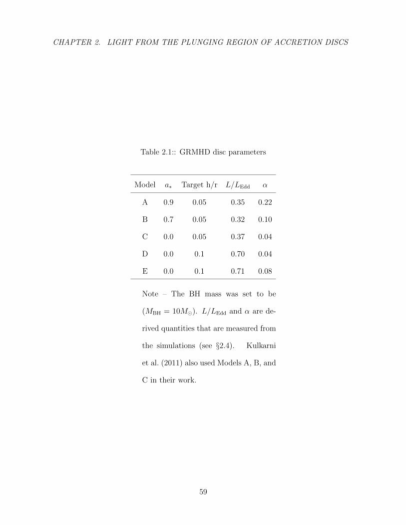
CHAPTER 2. LIGHT FROM THE PLUNGING REGION OF ACCRETION DISCS
Table 2.1:: GRMHD disc parameters
Model a∗ Target h/r L/LEdd α
A 0.9 0.05 0.35 0.22
B 0.7 0.05 0.32 0.10
C 0.0 0.05 0.37 0.04
D 0.0 0.1 0.70 0.04
E 0.0 0.1 0.71 0.08
Note – The BH mass was set to be
(MBH = 10M). L/LEdd and α are de-
rived quantities that are measured from
the simulations (see §2.4). Kulkarni
et al. (2011) also used Models A, B, and
C in their work.
59
CHAPTER 2. LIGHT FROM THE PLUNGING REGION OF ACCRETION DISCS
annulus. The blackbody is modified such that the specific intensity is given by:
Iν(T ) = f−4Bν(fT ), (2.2)
where Bν(T ) is the standard Planck function and f is spectral hardening constant (often
assumed to be 1.7 for X-ray binaries). Following Davis & Hubeny (2006), we improve
on this assumption by solving the radiative transfer equation. The emergent spectrum
for each annulus is obtained through the stellar atmospheres code tlusty (Hubeny &
Lanz 1995). The code simultaneously solves for the vertical structure of a plane-parallel
atmosphere and its angle dependent radiation field, and is independent of any blackbody
assumption. The atmosphere is modelled as a series of 1D vertical cells that are in
radiative, hydrostatic, and statistical equilibrium (which allows for departures from local
thermodynamic equilibrium in the atomic populations). In each cell, we obtain: the
spectrum as a function of viewing angle Iν(θ), density ρ, gas temperature T , vertical
height above the midplane z, and the particle composition (ne, nHI, n
HII, etc...).
We are primarily interested in each annulus’ emergent spectrum (i.e. Iν(θ) for the
surface cell). To obtain a unique solution in the stellar atmospheres problem, we need to
specify the following 3 boundary conditions:
(1). The radiative cooling flux F = σSBT4eff (where Teff is the annulus effective
temperature).
(2). The vertical tidal gravity experienced by the fluid (parametrized by Q = g⊥/z
where g⊥ is the vertical acceleration and z is the height above the midplane).
60

CHAPTER 2. LIGHT FROM THE PLUNGING REGION OF ACCRETION DISCS
(3). The column density to the midplane m = Σ/2 (where Σ is the total column density
of the annulus).
In the framework of tlusty, the problem of computing the disc spectrum simply
becomes one of obtaining the radial profiles of Teff(r), Q(r), and m(r) for the GRMHD
disc. We compute the spectrum for each disc annulus using the corresponding values of
Teff , Q, and m.
2.3.1 Assumptions in the TLUSTY model
In our annulus problem, we make the assumption of uniform viscous heating per
unit mass, and we ignore the effects of magnetic pressure support, fluid convection,
and heat conduction. We allow for deviations from LTE by explicitly computing the
ion populations for H, He, C, N, O, Ne, Mg, Si, S, Ar, Ca, and Fe assuming solar
abundances. In the non-LTE calculations, only the lowest energy level is considered for
each ionization state, except for the cases of H and He+, which are modelled with 9
and 4 levels respectively. The treatment of bound-free transitions include all outer shell
ionization processes, collisional excitations, and an approximate treatment for Auger
(inner shell) processes. Free-bound processes modelled include radiative, dielectric, and
three-body recombination. Free-free transitions are modelled for all listed elements,
whereas bound-bound transitions are not modelled. Comptonization is included through
an angle-averaged Kompaneets treatment (Hubeny et al. 2001). Finally, to reduce the
number of independent vertical cells in the problem, we assume that the annulus is
symmetric about the midplane.
One drawback of the algorithm used in tlusty (lambda-iteration and complete
61

CHAPTER 2. LIGHT FROM THE PLUNGING REGION OF ACCRETION DISCS
linearization, see Hubeny & Lanz 1995 for details) is that tlusty requires an initial
guess for the conditions in each vertical cell. The code often fails to converge when
the initial guess is poor. However, if tlusty finds a converged solution, it is robust
to the choice of initial guess. Often, manual intervention (in the form of providing
better initial guesses) is needed to ensure convergence, which means that the process
of generating annuli spectra cannot be completely automated. However, since only
three parameters are necessary to uniquely specify an annulus, we have simply manually
precomputed a grid of annuli spanning the full range of parameter space for the case
of stellar mass black hole systems. The grid spans log10 Teff ∈ 5.5, 5.6, . . . , 7.3,
log10Q ∈ −4.0, −3.9, . . . , 9.0, and log10m ∈ 0.5, 0.6, . . . , 2.8, 2.9, 3.0, 4.0, 5.0, 6.0.
We then interpolate on this grid to obtain any needed annuli spectra (see Appendix 2.11
for details on the interpolation process).
2.4 Slicing the GRMHD disc into Annuli
Since we wish to describe the accretion disc from the 3D GRMHD simulations as a series
of annuli, we take out the poloidal and toroidal structure through an averaging process.
All quantities are first subject to azimuthal averaging (since we model the annuli as
azimuthally symmetric structures), followed by vertical averaging (i.e. averaging over
θ) weighted by rest mass density. For each annulus in the GRMHD simulation, we
must identify Teff(r), Q(r), and Σ(r) before we can call on tlusty to provide the local
spectrum.
We obtain Teff(r) directly from the simulation luminosity profile (§2.4.1), Q(r) from
the Kerr metric and the fluid velocities (§2.4.2), and Σ(r) from the fluid velocities and
62
CHAPTER 2. LIGHT FROM THE PLUNGING REGION OF ACCRETION DISCS
accretion rate (§2.4.3). Since the simulations are dimensionless, we must first choose a
black hole mass M and a disc luminosity L/LEdd to dimensionalize the radial profiles
of Teff(r), Q(r), and Σ(r). For all the simulation runs, we have chosen a fiducial value
of M = 10 M, and we set L/LEdd so the disc thickness in the radiative model matches
that of the GRMHD simulation (see §2.4.1).
One complicating factor is that the simulated disc is only reliable for a short range
of radii. Beyond a certain critical radius r > rie (where rie stands for the radius of inflow
equilibrium – see Penna et al. 2010 for a detailed discussion), the simulation has not
been run long enough for the fluid to reach its equilibrium configuration. The relevant
physical time-scale for reaching inflow equilibrium is the accretion time tacc = r/ur,
where ur is the fluid’s radial velocity. The problem with fluid outside of rie is that this
fluid still has memory of its initial conditions (i.e. fluid outside of rie has tacc > tsim,
where tsim is the total runtime of the simulation). Beyond the inflow equilibrium point,
we instead turn to an analytic disc model that is matched to the simulation disc (we use
a generalized NT model that allows for nonzero stresses at the ISCO, see Appendices
2.9 and 2.10 for details). The analytic model also requires us to specify a disc viscosity
parameter α (defined as the ratio between the vertically integrated stress and pressure,
see Novikov & Thorne 1973). Table 2.1 lists the values of L/LEdd and α corresponding
to the different simulation runs, where both parameters are determined by matching the
GRMHD disc at rie to the analytic generalized NT disc (see §2.4.1 and §2.4.3).
63
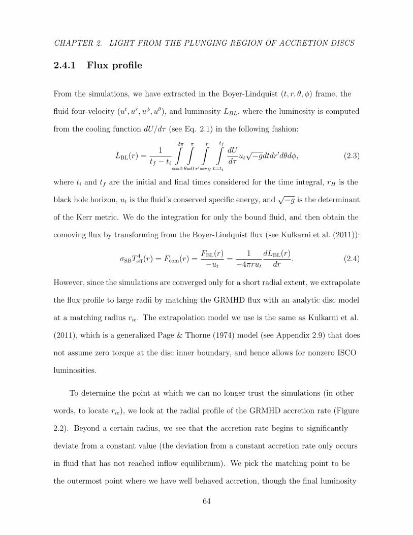
CHAPTER 2. LIGHT FROM THE PLUNGING REGION OF ACCRETION DISCS
2.4.1 Flux profile
From the simulations, we have extracted in the Boyer-Lindquist (t, r, θ, φ) frame, the
fluid four-velocity (ut, ur, uφ, uθ), and luminosity LBL, where the luminosity is computed
from the cooling function dU/dτ (see Eq. 2.1) in the following fashion:
LBL(r) =1
tf − ti
2π∫φ=0
π∫θ=0
r∫r′=rH
tf∫t=ti
dU
dτut√−gdtdr′dθdφ, (2.3)
where ti and tf are the initial and final times considered for the time integral, rH is the
black hole horizon, ut is the fluid’s conserved specific energy, and√−g is the determinant
of the Kerr metric. We do the integration for only the bound fluid, and then obtain the
comoving flux by transforming from the Boyer-Lindquist flux (see Kulkarni et al. (2011)):
σSBT4eff(r) = Fcom(r) =
FBL(r)
−ut=
1
−4πrut
dLBL(r)
dr. (2.4)
However, since the simulations are converged only for a short radial extent, we extrapolate
the flux profile to large radii by matching the GRMHD flux with an analytic disc model
at a matching radius rie. The extrapolation model we use is the same as Kulkarni et al.
(2011), which is a generalized Page & Thorne (1974) model (see Appendix 2.9) that does
not assume zero torque at the disc inner boundary, and hence allows for nonzero ISCO
luminosities.
To determine the point at which we can no longer trust the simulations (in other
words, to locate rie), we look at the radial profile of the GRMHD accretion rate (Figure
2.2). Beyond a certain radius, we see that the accretion rate begins to significantly
deviate from a constant value (the deviation from a constant accretion rate only occurs
in fluid that has not reached inflow equilibrium). We pick the matching point to be
the outermost point where we have well behaved accretion, though the final luminosity
64
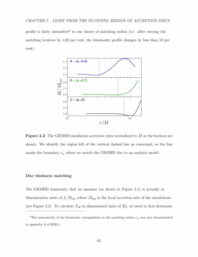
CHAPTER 2. LIGHT FROM THE PLUNGING REGION OF ACCRETION DISCS
profile is fairly insensitive6 to our choice of matching radius (i.e. after varying the
matching location by ±20 per cent, the luminosity profile changes by less than 10 per
cent).
Figure 2.2: The GRMHD simulation accretion rates normalized to M at the horizon are
shown. We identify the region left of the vertical dashed line as converged, so the line
marks the boundary rie where we match the GRMHD disc to an analytic model.
Disc thickness matching
The GRMHD luminosity that we measure (as shown in Figure 2.1) is actually in
dimensionless units of L/Msim where Msim is the local accretion rate of the simulations
(see Figure 2.2). To calculate Teff in dimensioned units of [K], we need to first determine
6The insensitivity of the luminosity extrapolation to the matching radius rie was also demonstrated
in appendix A of K2011.
65
CHAPTER 2. LIGHT FROM THE PLUNGING REGION OF ACCRETION DISCS
the dimensioned luminosity corresponding to the GRMHD simulations. Unfortunately,
the simulations do not include radiation physics, so the simulation fluid does not have a
set density scale, which means there is no direct way of measuring M and hence L. We
thus resort to an indirect method for determining this accretion rate. We identify L/LEdd
of the simulation with the value that matches the disc thickness in both the GRMHD
simulated disc and the tlusty annuli7 (see Figure 2.3). However, since tlusty ignores
magnetic support and the simulations ignore radiation pressure, the tlusty based
and GRMHD thickness profiles have completely different shapes. We opt to match the
thickness at the radius corresponding to the luminosity peak (see Figure 2.3).
Although the luminosity profile drops off fairly rapidly inside the ISCO (see Fig.
2.1), we find that the disc’s effective temperature remains roughly constant (Fig. 2.4).
Therefore the falloff in disc luminosity when approaching the BH horizon is purely
a geometric effect. Annuli near the horizon have less surface area, and hence they
contribute less to the total luminosity.
7Kulkarni et al. (2011) also applied this method to dimensionalize their luminosity profiles
66
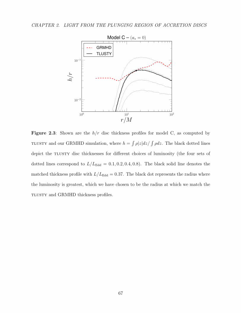
CHAPTER 2. LIGHT FROM THE PLUNGING REGION OF ACCRETION DISCS
Figure 2.3: Shown are the h/r disc thickness profiles for model C, as computed by
tlusty and our GRMHD simulation, where h =∫ρ|z|dz/
∫ρdz. The black dotted lines
depict the tlusty disc thicknesses for different choices of luminosity (the four sets of
dotted lines correspond to L/LEdd = 0.1, 0.2, 0.4, 0.8). The black solid line denotes the
matched thickness profile with L/LEdd = 0.37. The black dot represents the radius where
the luminosity is greatest, which we have chosen to be the radius at which we match the
tlusty and GRMHD thickness profiles.
67
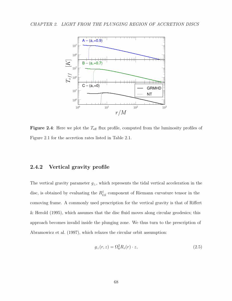
CHAPTER 2. LIGHT FROM THE PLUNGING REGION OF ACCRETION DISCS
Figure 2.4: Here we plot the Teff flux profile, computed from the luminosity profiles of
Figure 2.1 for the accretion rates listed in Table 2.1.
2.4.2 Vertical gravity profile
The vertical gravity parameter g⊥, which represents the tidal vertical acceleration in the
disc, is obtained by evaluating the Rztzt
component of Riemann curvature tensor in the
comoving frame. A commonly used prescription for the vertical gravity is that of Riffert
& Herold (1995), which assumes that the disc fluid moves along circular geodesics; this
approach becomes invalid inside the plunging zone. We thus turn to the prescription of
Abramowicz et al. (1997), which relaxes the circular orbit assumption:
g⊥(r, z) = Ω2kRz(r) · z, (2.5)
68
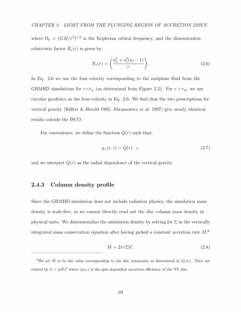
CHAPTER 2. LIGHT FROM THE PLUNGING REGION OF ACCRETION DISCS
where Ωk = (GM/r3)1/2 is the Keplerian orbital frequency, and the dimensionless
relativistic factor Rz(r) is given by:
Rz(r) =
(u2φ + a2
∗(ut − 1)
r
). (2.6)
In Eq. 2.6 we use the four-velocity corresponding to the midplane fluid from the
GRMHD simulations for r<rie (as determined from Figure 2.2). For r > rie, we use
circular geodesics as the four-velocity in Eq. 2.6. We find that the two prescriptions for
vertical gravity (Riffert & Herold 1995; Abramowicz et al. 1997) give nearly identical
results outside the ISCO.
For convenience, we define the function Q(r) such that:
g⊥(r, z) = Q(r) · z, (2.7)
and we interpret Q(r) as the radial dependence of the vertical gravity.
2.4.3 Column density profile
Since the GRMHD simulation does not include radiation physics, the simulation mass
density is scale-free, so we cannot directly read out the disc column mass density in
physical units. We dimensionalize the simulation density by solving for Σ in the vertically
integrated mass conservation equation after having picked a constant accretion rate M :8
M = 2πrΣur, (2.8)
8We set M to be the value corresponding to the disc luminosity as determined in §2.4.1. They are
related by L = ηMc2 where η(a∗) is the spin dependent accretion efficiency of the NT disc.
69
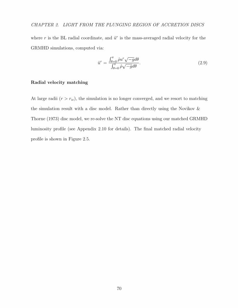
CHAPTER 2. LIGHT FROM THE PLUNGING REGION OF ACCRETION DISCS
where r is the BL radial coordinate, and ur is the mass-averaged radial velocity for the
GRMHD simulations, computed via:
ur =
∫ πθ=0
ρur√−gdθ∫ π
θ=0ρ√−gdθ
. (2.9)
Radial velocity matching
At large radii (r > rie), the simulation is no longer converged, and we resort to matching
the simulation result with a disc model. Rather than directly using the Novikov &
Thorne (1973) disc model, we re-solve the NT disc equations using our matched GRMHD
luminosity profile (see Appendix 2.10 for details). The final matched radial velocity
profile is shown in Figure 2.5.
70
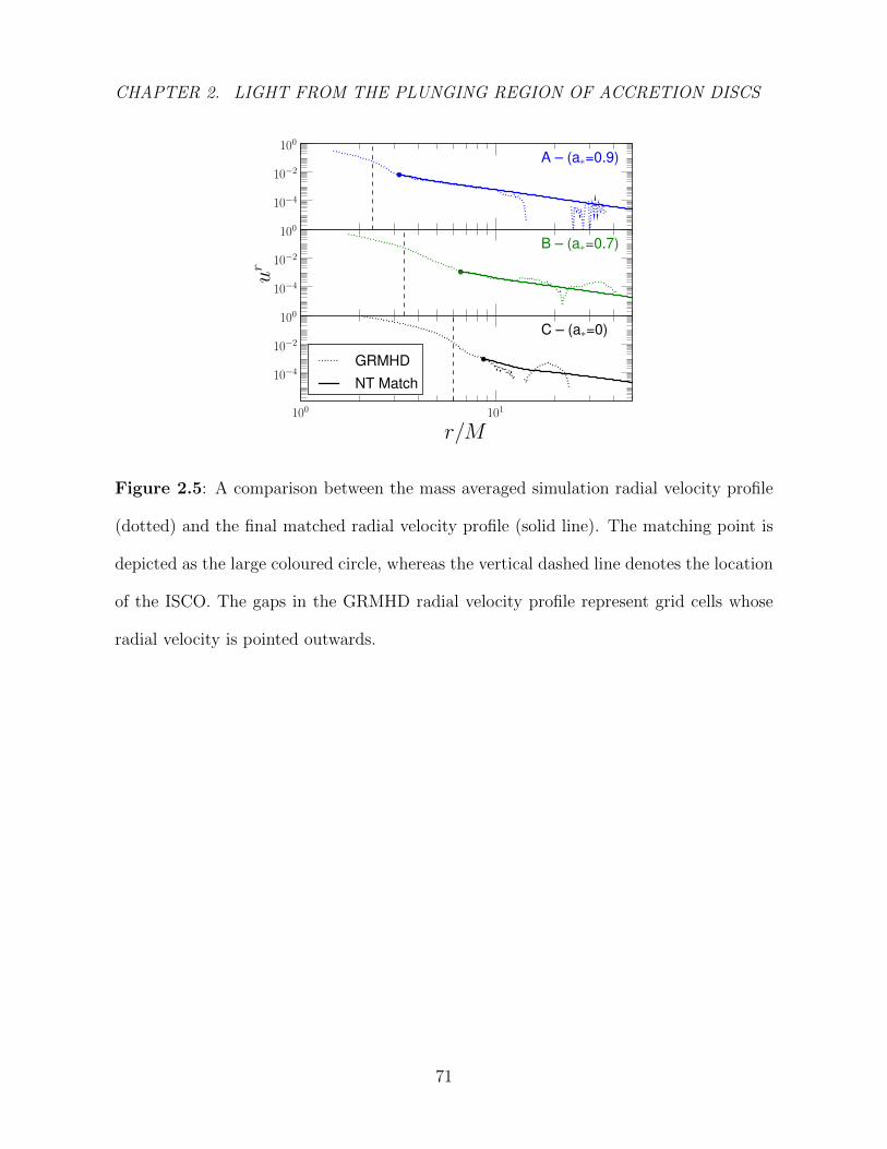
CHAPTER 2. LIGHT FROM THE PLUNGING REGION OF ACCRETION DISCS
Figure 2.5: A comparison between the mass averaged simulation radial velocity profile
(dotted) and the final matched radial velocity profile (solid line). The matching point is
depicted as the large coloured circle, whereas the vertical dashed line denotes the location
of the ISCO. The gaps in the GRMHD radial velocity profile represent grid cells whose
radial velocity is pointed outwards.
71
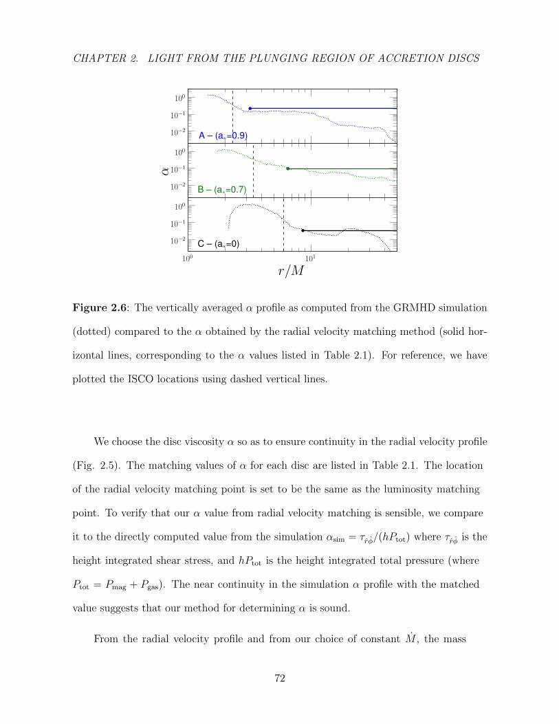
CHAPTER 2. LIGHT FROM THE PLUNGING REGION OF ACCRETION DISCS
Figure 2.6: The vertically averaged α profile as computed from the GRMHD simulation
(dotted) compared to the α obtained by the radial velocity matching method (solid hor-
izontal lines, corresponding to the α values listed in Table 2.1). For reference, we have
plotted the ISCO locations using dashed vertical lines.
We choose the disc viscosity α so as to ensure continuity in the radial velocity profile
(Fig. 2.5). The matching values of α for each disc are listed in Table 2.1. The location
of the radial velocity matching point is set to be the same as the luminosity matching
point. To verify that our α value from radial velocity matching is sensible, we compare
it to the directly computed value from the simulation αsim = τrφ/(hPtot) where τrφ is the
height integrated shear stress, and hPtot is the height integrated total pressure (where
Ptot = Pmag + Pgas). The near continuity in the simulation α profile with the matched
value suggests that our method for determining α is sound.
From the radial velocity profile and from our choice of constant M , the mass
72
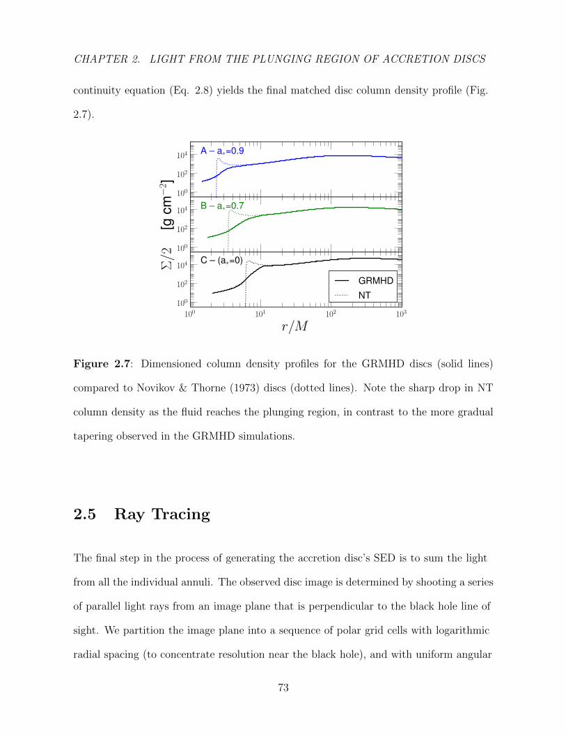
CHAPTER 2. LIGHT FROM THE PLUNGING REGION OF ACCRETION DISCS
continuity equation (Eq. 2.8) yields the final matched disc column density profile (Fig.
2.7).
Figure 2.7: Dimensioned column density profiles for the GRMHD discs (solid lines)
compared to Novikov & Thorne (1973) discs (dotted lines). Note the sharp drop in NT
column density as the fluid reaches the plunging region, in contrast to the more gradual
tapering observed in the GRMHD simulations.
2.5 Ray Tracing
The final step in the process of generating the accretion disc’s SED is to sum the light
from all the individual annuli. The observed disc image is determined by shooting a series
of parallel light rays from an image plane that is perpendicular to the black hole line of
sight. We partition the image plane into a sequence of polar grid cells with logarithmic
radial spacing (to concentrate resolution near the black hole), and with uniform angular
73
CHAPTER 2. LIGHT FROM THE PLUNGING REGION OF ACCRETION DISCS
spacing. To produce the ray traced images, we shoot rays for Nr = 300 radial grid cells
and Nφ = 100 polar cells. The grid is then further squashed by a factor of cos i to match
the geometry of the inclined disc.
A single ray is shot for each grid cell, and by numerically integrating the
(second-order) geodesic equations for light:
d2xα
dλ2+ Γαβγ
dxβ
dλ
dxγ
λ= 0, (2.10)
where λ is an affine parameter along the geodesic, and Γαβγ are the connection coefficients,
we locate the first disc midplane intersection for each light ray (we stop at the disc
midplane since we have an optically thick disc – see Figure 2.11 for a plot of the optical
depth profile). For simplicity, we opt to use the disc midplane as the point of light
emission rather than using the annuli’s precise photosphere. Kulkarni et al. (2011)
has suggested that this effect only becomes important for thick discs viewed at high
inclinations angles (which is when disc self-shadowing becomes important). In this work,
we do not expect the distinction between midplane and photosphere to be important
since we are dealing with thin discs (where h/r cos i). This process of following the
trajecories of multiple rays of light to produce an image is called ‘ray tracing’. The ray
tracing code used in this work was originally developed by Scherbakov & Huang (2011),
with further refinements by Kulkarni et al. (2011).
We then compute (by interpolation on the GRMHD grid cells, see Appendix 2.11
for details) the local values of: flux Teff , column density Σ, vertical gravity Q, and
comoving light ray incidence angle µ. The local comoving spectrum is then obtained by
interpolating on our grid of tlusty atmosphere models. We then apply the relevant
Doppler boosting and gravitational redshifting to these spectra (see Fig. 2.8 for the ray
74
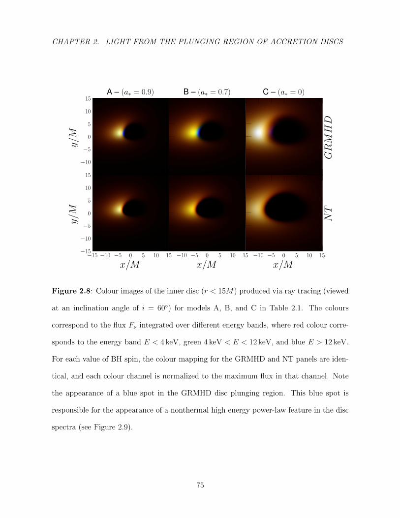
CHAPTER 2. LIGHT FROM THE PLUNGING REGION OF ACCRETION DISCS
Figure 2.8: Colour images of the inner disc (r < 15M) produced via ray tracing (viewed
at an inclination angle of i = 60) for models A, B, and C in Table 2.1. The colours
correspond to the flux Fν integrated over different energy bands, where red colour corre-
sponds to the energy band E < 4 keV, green 4 keV < E < 12 keV, and blue E > 12 keV.
For each value of BH spin, the colour mapping for the GRMHD and NT panels are iden-
tical, and each colour channel is normalized to the maximum flux in that channel. Note
the appearance of a blue spot in the GRMHD disc plunging region. This blue spot is
responsible for the appearance of a nonthermal high energy power-law feature in the disc
spectra (see Figure 2.9).
75
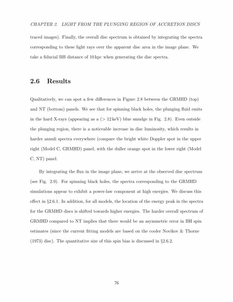
CHAPTER 2. LIGHT FROM THE PLUNGING REGION OF ACCRETION DISCS
traced images). Finally, the overall disc spectrum is obtained by integrating the spectra
corresponding to these light rays over the apparent disc area in the image plane. We
take a fiducial BH distance of 10 kpc when generating the disc spectra.
2.6 Results
Qualitatively, we can spot a few differences in Figure 2.8 between the GRMHD (top)
and NT (bottom) panels. We see that for spinning black holes, the plunging fluid emits
in the hard X-rays (appearing as a (> 12 keV) blue smudge in Fig. 2.8). Even outside
the plunging region, there is a noticeable increase in disc luminosity, which results in
harder annuli spectra everywhere (compare the bright white Doppler spot in the upper
right (Model C, GRMHD) panel, with the duller orange spot in the lower right (Model
C, NT) panel.
By integrating the flux in the image plane, we arrive at the observed disc spectrum
(see Fig. 2.9). For spinning black holes, the spectra corresponding to the GRMHD
simulations appear to exhibit a power-law component at high energies. We discuss this
effect in §2.6.1. In addition, for all models, the location of the energy peak in the spectra
for the GRMHD discs is shifted towards higher energies. The harder overall spectrum of
GRMHD compared to NT implies that there would be an asymmetric error in BH spin
estimates (since the current fitting models are based on the cooler Novikov & Thorne
(1973) disc). The quantitative size of this spin bias is discussed in §2.6.2.
76
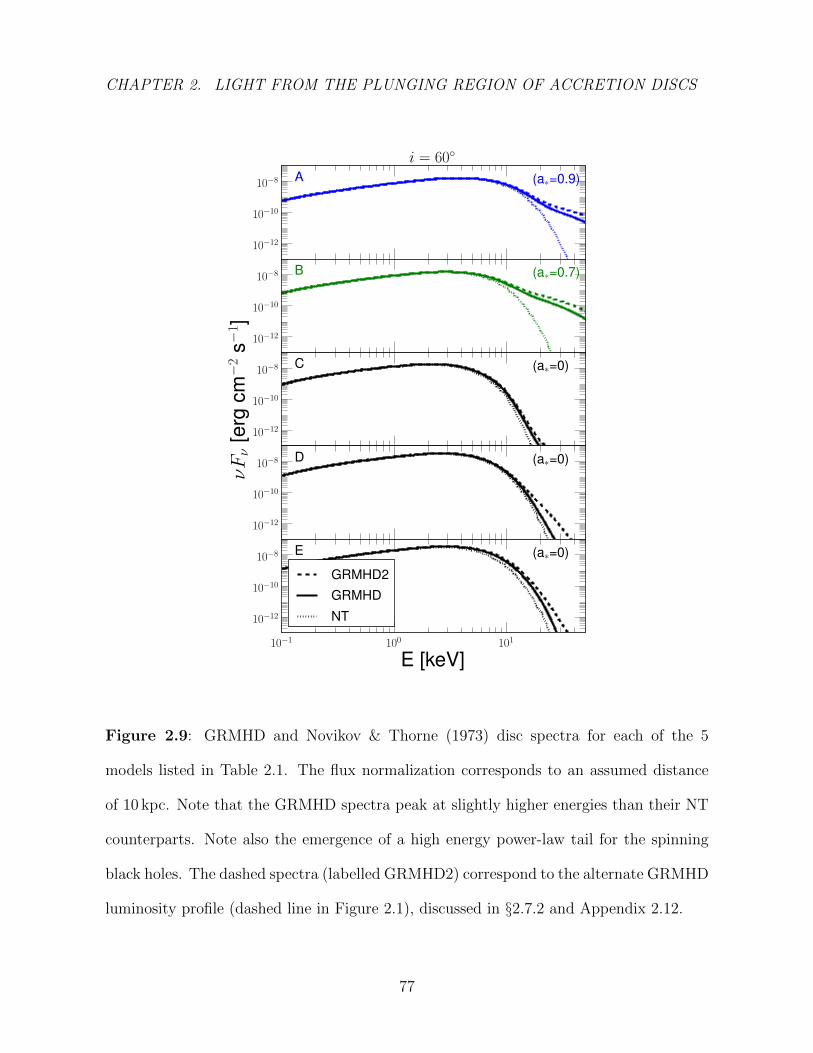
CHAPTER 2. LIGHT FROM THE PLUNGING REGION OF ACCRETION DISCS
Figure 2.9: GRMHD and Novikov & Thorne (1973) disc spectra for each of the 5
models listed in Table 2.1. The flux normalization corresponds to an assumed distance
of 10 kpc. Note that the GRMHD spectra peak at slightly higher energies than their NT
counterparts. Note also the emergence of a high energy power-law tail for the spinning
black holes. The dashed spectra (labelled GRMHD2) correspond to the alternate GRMHD
luminosity profile (dashed line in Figure 2.1), discussed in §2.7.2 and Appendix 2.12.
77
CHAPTER 2. LIGHT FROM THE PLUNGING REGION OF ACCRETION DISCS
2.6.1 Power law tail
Observationally, high-energy power-law tails are often seen in the X-ray spectra of black
hole binary systems (e.g. Miyamoto et al. 1991; McClintock et al. 2001; Reis et al. 2010).
The current leading theory to explain these high-energy power-law phenomena is the
action of a hot optically thin corona (Zhang et al. 1997b), which produces the power-law
tail by means of either Comptonization of disc photons, synchrotron radiation, and/or
synchrotron self-Comptonization (Miller 2007; McClintock & Remillard 2006). Despite
the many proposed coronal models (e.g. Haardt & Maraschi 1991; Dove et al. 1997;
Kawaguchi et al. 2000; Liu et al. 2002), there is no agreed-upon standard (i.e. there is
scarce agreement on the geometry and physical properties of the corona). Although a
hot corona is often invoked to explain the existence of a high energy power-law tail, in
this work we naturally recover a hot power-law tail from just the thermal disc fluid that
occupies the plunging region.
To better understand the origin of the apparent high-energy power-law tail in our
models, we examine the area-weighted local spectrum for several annuli in model B
(a∗ = 0.7), chosen since this simulated disc exhibits the strongest tail relative to the disc
continuum. From Figure 2.10, we see that the high energy power-law tail stems solely
from the emission of annuli inside the plunging region (coloured in blue). Furthermore,
we see that the power-law emerges from the combined emission of plunging annuli
at various locations (i.e. the envelope of spectra from r = 2M − 3M comprise the
power-law). No single annulus emits the full power-law.
In our plunging region model, we find that the strength of the high energy power-law
also depends on BH spin. The spinless models (C, D, E) do not appear to produce any
78
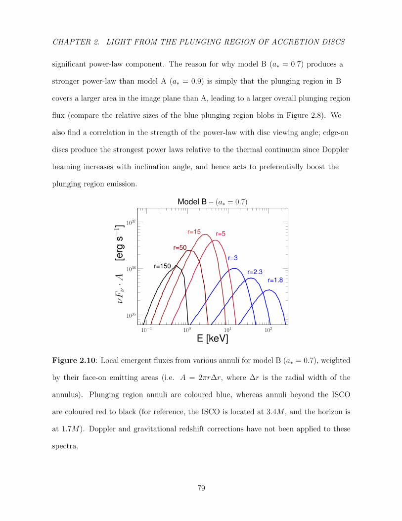
CHAPTER 2. LIGHT FROM THE PLUNGING REGION OF ACCRETION DISCS
significant power-law component. The reason for why model B (a∗ = 0.7) produces a
stronger power-law than model A (a∗ = 0.9) is simply that the plunging region in B
covers a larger area in the image plane than A, leading to a larger overall plunging region
flux (compare the relative sizes of the blue plunging region blobs in Figure 2.8). We
also find a correlation in the strength of the power-law with disc viewing angle; edge-on
discs produce the strongest power laws relative to the thermal continuum since Doppler
beaming increases with inclination angle, and hence acts to preferentially boost the
plunging region emission.
Figure 2.10: Local emergent fluxes from various annuli for model B (a∗ = 0.7), weighted
by their face-on emitting areas (i.e. A = 2πr∆r, where ∆r is the radial width of the
annulus). Plunging region annuli are coloured blue, whereas annuli beyond the ISCO
are coloured red to black (for reference, the ISCO is located at 3.4M , and the horizon is
at 1.7M). Doppler and gravitational redshift corrections have not been applied to these
spectra.
79

CHAPTER 2. LIGHT FROM THE PLUNGING REGION OF ACCRETION DISCS
We find that the spectral hardening factor for the plunging annuli appears to start
growing non-linearly as the gas approaches the horizon (see Fig. 2.10 and note the rapid
shift in the spectral peak locations for the blue plunging region annuli, despite that Teff
is nearly constant in the plunging zone as per Fig. 2.4). The physical reason for this
rapid spectral hardening is simply that the plunging gas quickly becomes extremely hot.
Upon entering the plunging region, the fast radial plunge causes the annuli to rapidly
thin out in column density. The dropping column mass allows the annuli to make the
transition from being optically thick to effectively optically thin9 (see Fig. 2.11). Despite
this drop in column density, the gas needs to maintain a roughly constant cooling rate
(i.e. Teff remains constant in the plunging zone – see Fig. 2.4). A property of effectively
optically thin gas is that it cannot radiate efficiently (Shapiro, Lightman, & Eardley
1976). To keep a constant cooling rate despite the rapidly dropping optical depth, the
gas must heat up tremendously, leading to very hot emission.
9An effectively optically thin medium is one that is optically thin to absorption, and optically thick
to scattering.
80
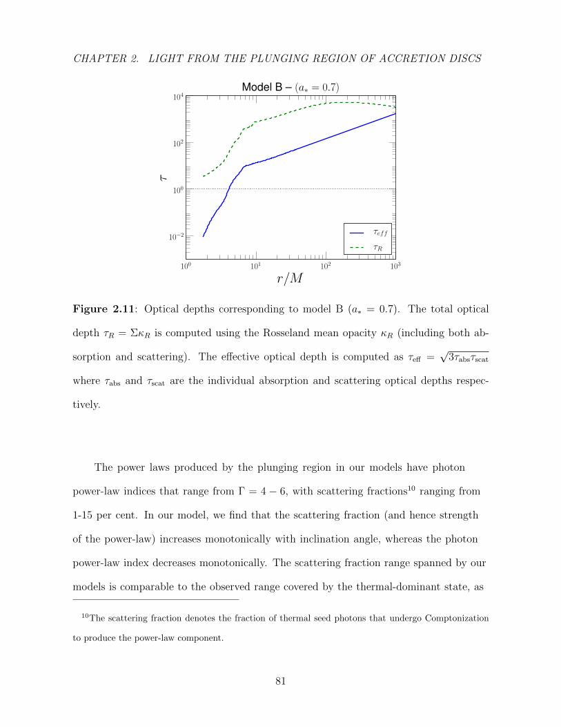
CHAPTER 2. LIGHT FROM THE PLUNGING REGION OF ACCRETION DISCS
Figure 2.11: Optical depths corresponding to model B (a∗ = 0.7). The total optical
depth τR = ΣκR is computed using the Rosseland mean opacity κR (including both ab-
sorption and scattering). The effective optical depth is computed as τeff =√
3τabsτscat
where τabs and τscat are the individual absorption and scattering optical depths respec-
tively.
The power laws produced by the plunging region in our models have photon
power-law indices that range from Γ = 4 − 6, with scattering fractions10 ranging from
1-15 per cent. In our model, we find that the scattering fraction (and hence strength
of the power-law) increases monotonically with inclination angle, whereas the photon
power-law index decreases monotonically. The scattering fraction range spanned by our
models is comparable to the observed range covered by the thermal-dominant state, as
10The scattering fraction denotes the fraction of thermal seed photons that undergo Comptonization
to produce the power-law component.
81
CHAPTER 2. LIGHT FROM THE PLUNGING REGION OF ACCRETION DISCS
well as much of the range of the intermediate, and steep power-law states for black hole
binaries (which ranges from 0-25 per cent – see Steiner et al. 2009b, 2011). However, even
in the steep power-law state, the observed photon index range of Γ = 2.2− 2.7(Gou et al.
2009, 2011; Steiner et al. 2011) is much less steep than what we predict with our plunging
region model. This discrepancy may simply be due to a limitation of our model, which
neglects the physics of disc self-irradiation. Including this effect would result in a hotter
disc that would act to boost the strength of the high energy tails. Also, self-irradiation
becomes increasingly important as you approach the black hole (where light bending is
most severe). This implies that including irradiation will likely result in power laws that
are less steep (since the emission from the hottest, innermost annuli will be boosted the
most by this self-irradiation effect). We speculate that a more complete treatment of the
plunging region (that includes the physics of disc irradiation and magnetic fields) would
produce high energy tails that are better matches to observations.
Since many of our approximations become poor in the plunging region (see §2.7
for a discussion of some of the pitfalls of our method), we strongly caution against
reading too much into the quantitative details of the power laws of Figure 2.9 (i.e. slope,
normalization). The high energy power-law result should be taken only at the qualitative
level; although the plunging region luminosity is dwarfed by the disc luminosity, it starts
to dominate the flux at E > 20 keV taking on a nonthermal shape that appears as a
power-law.
82
CHAPTER 2. LIGHT FROM THE PLUNGING REGION OF ACCRETION DISCS
2.6.2 Quantitative effect on spin
As already discussed, the thermal emission from the disc is slightly stronger and hotter
in the GRMHD models compared to the equivalent NT model. This will introduce an
error in BH spin estimates obtained from the continuum fitting method. To precisely
quantify the effect, we generate mock observations of our GRMHD discs and we fit these
simulated observations with the currently used suite of continuum-fitting disc models.
For simplicity, to generate these mock observations, we use an idealized instrument with
effective area that is independent of photon energy. We choose the instrument’s effective
area11 to be 1000 cm2, and use a 3h exposure time. We compute photon statistics in
1000 energy channels uniformly spaced in logE, ranging from 0.4 keV < E < 50.0 keV.
We then fit our simulated disc observations with bhspec (Davis et al. 2005; Davis &
Hubeny 2006), which is a set of (TLUSTY based) disc spectra often used in continuum
fitting. The bhspec spectra are computed in much the same way as our procedure in
§2.1, except that bhspec uses a classic Novikov & Thorne (1973) disc instead of our
GRMHD disc. Whenever necessary, we also attempt to fit a power-law tail to the models
using simpl (Steiner et al. 2009a), which is a physically motivated Comptonization
model that has been quite successful in fitting many observed high energy power-law
tails (Steiner et al. 2009b).
11This is modelled after the Rossi X-Ray Timing Explorer’s total effective area in the hard energy band
(> 20 keV), see Jahoda et al. (2006)
83
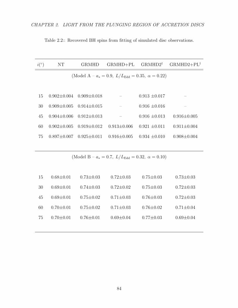
CHAPTER 2. LIGHT FROM THE PLUNGING REGION OF ACCRETION DISCS
Table 2.2:: Recovered BH spins from fitting of simulated disc observations.
i() NT GRMHD GRMHD+PL GRMHD2† GRMHD2+PL†
(Model A – a∗ = 0.9, L/LEdd = 0.35, α = 0.22)
15 0.902±0.004 0.909±0.018 – 0.913 ±0.017 –
30 0.909±0.005 0.914±0.015 – 0.916 ±0.016 –
45 0.904±0.006 0.912±0.013 – 0.916 ±0.013 0.916±0.005
60 0.902±0.005 0.919±0.012 0.913±0.006 0.921 ±0.011 0.911±0.004
75 0.897±0.007 0.925±0.011 0.916±0.005 0.934 ±0.010 0.908±0.004
(Model B – a∗ = 0.7, L/LEdd = 0.32, α = 0.10)
15 0.68±0.01 0.73±0.03 0.72±0.03 0.75±0.03 0.73±0.03
30 0.69±0.01 0.74±0.03 0.72±0.02 0.75±0.03 0.72±0.03
45 0.69±0.01 0.75±0.02 0.71±0.03 0.76±0.03 0.72±0.03
60 0.70±0.01 0.75±0.02 0.71±0.03 0.76±0.02 0.71±0.04
75 0.70±0.01 0.76±0.01 0.69±0.04 0.77±0.03 0.69±0.04
84
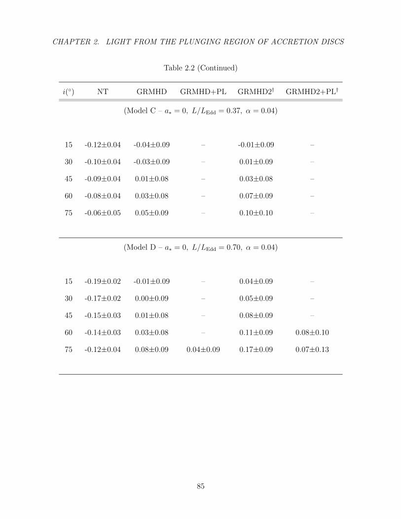
CHAPTER 2. LIGHT FROM THE PLUNGING REGION OF ACCRETION DISCS
Table 2.2 (Continued)
i() NT GRMHD GRMHD+PL GRMHD2† GRMHD2+PL†
(Model C – a∗ = 0, L/LEdd = 0.37, α = 0.04)
15 -0.12±0.04 -0.04±0.09 – -0.01±0.09 –
30 -0.10±0.04 -0.03±0.09 – 0.01±0.09 –
45 -0.09±0.04 0.01±0.08 – 0.03±0.08 –
60 -0.08±0.04 0.03±0.08 – 0.07±0.09 –
75 -0.06±0.05 0.05±0.09 – 0.10±0.10 –
(Model D – a∗ = 0, L/LEdd = 0.70, α = 0.04)
15 -0.19±0.02 -0.01±0.09 – 0.04±0.09 –
30 -0.17±0.02 0.00±0.09 – 0.05±0.09 –
45 -0.15±0.03 0.01±0.08 – 0.08±0.09 –
60 -0.14±0.03 0.03±0.08 – 0.11±0.09 0.08±0.10
75 -0.12±0.04 0.08±0.09 0.04±0.09 0.17±0.09 0.07±0.13
85
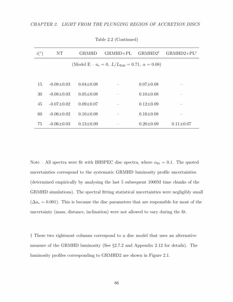
CHAPTER 2. LIGHT FROM THE PLUNGING REGION OF ACCRETION DISCS
Table 2.2 (Continued)
i() NT GRMHD GRMHD+PL GRMHD2† GRMHD2+PL†
(Model E – a∗ = 0, L/LEdd = 0.71, α = 0.08)
15 -0.08±0.03 0.04±0.08 – 0.07±0.08 –
30 -0.08±0.03 0.05±0.08 – 0.10±0.08 –
45 -0.07±0.02 0.09±0.07 – 0.12±0.09 –
60 -0.06±0.02 0.10±0.08 – 0.16±0.08 –
75 -0.06±0.03 0.13±0.09 – 0.20±0.09 0.11±0.07
Note – All spectra were fit with BHSPEC disc spectra, where αfit = 0.1. The quoted
uncertainties correspond to the systematic GRMHD luminosity profile uncertainties
(determined empirically by analysing the last 5 subsequent 1000M time chunks of the
GRMHD simulations). The spectral fitting statistical uncertainties were negligibly small
(∆a∗ ∼ 0.001). This is because the disc parameters that are responsible for most of the
uncertainty (mass, distance, inclination) were not allowed to vary during the fit.
† These two rightmost columns correspond to a disc model that uses an alternative
measure of the GRMHD luminosity (See §2.7.2 and Appendix 2.12 for details). The
luminosity profiles corresponding to GRMHD2 are shown in Figure 2.1.
86
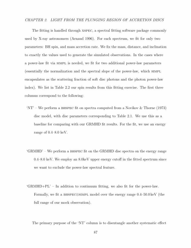
CHAPTER 2. LIGHT FROM THE PLUNGING REGION OF ACCRETION DISCS
The fitting is handled through xspec, a spectral fitting software package commonly
used by X-ray astronomers (Arnaud 1996). For each spectrum, we fit for only two
parameters: BH spin, and mass accretion rate. We fix the mass, distance, and inclination
to exactly the values used to generate the simulated observations. In the cases where
a power-law fit via simpl is needed, we fit for two additional power-law parameters
(essentially the normalization and the spectral slope of the power-law, which simpl
encapsulates as the scattering fraction of soft disc photons and the photon power-law
index). We list in Table 2.2 our spin results from this fitting exercise. The first three
columns correspond to the following:
‘NT’ – We perform a bhspec fit on spectra computed from a Novikov & Thorne (1973)
disc model, with disc parameters corresponding to Table 2.1. We use this as a
baseline for comparing with our GRMHD fit results. For the fit, we use an energy
range of 0.4–8.0 keV.
‘GRMHD’ – We perform a bhspec fit on the GRMHD disc spectra on the energy range
0.4–8.0 keV. We employ an 8.0keV upper energy cutoff in the fitted spectrum since
we want to exclude the power-law spectral feature.
‘GRMHD+PL’ – In addition to continuum fitting, we also fit for the power-law.
Formally, we fit a bhspec⊗simpl model over the energy range 0.4–50.0 keV (the
full range of our mock observation).
The primary purpose of the ‘NT’ column is to disentangle another systematic effect
87
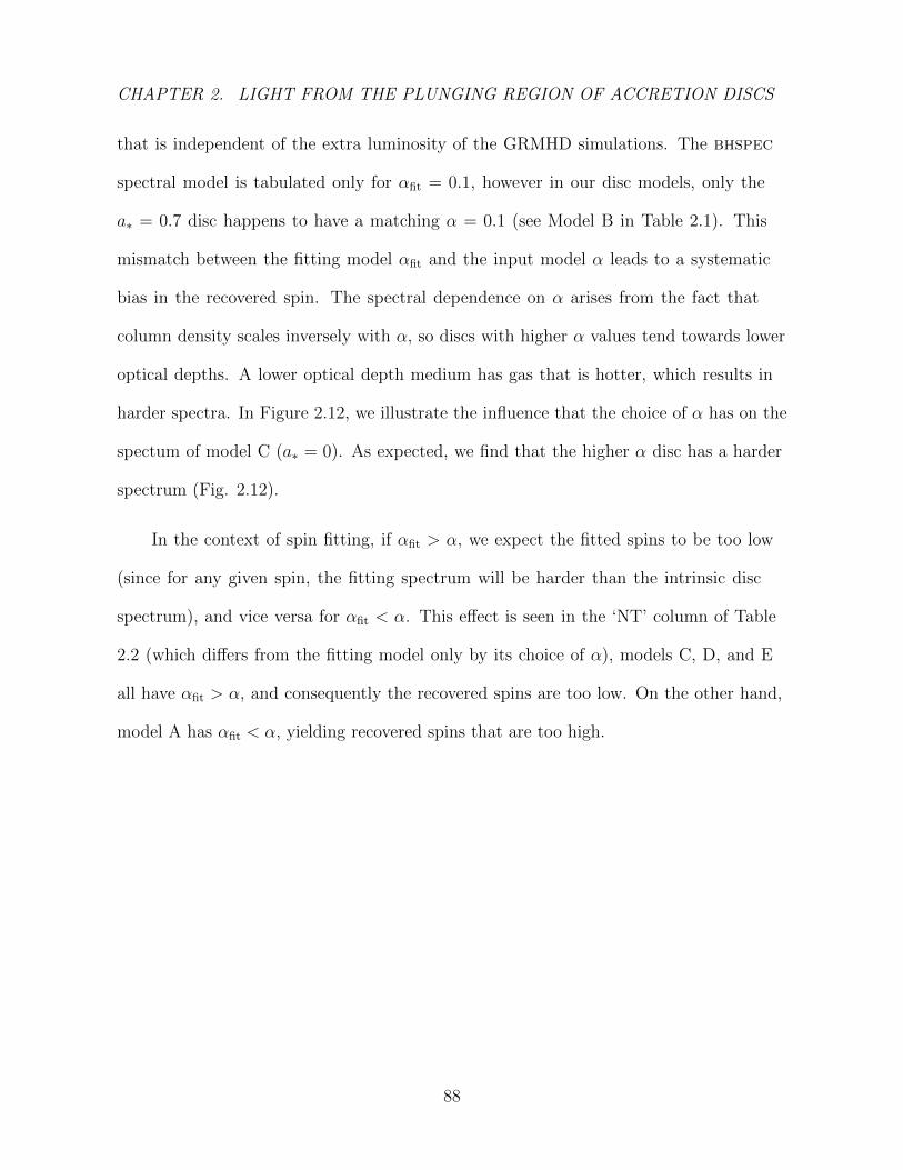
CHAPTER 2. LIGHT FROM THE PLUNGING REGION OF ACCRETION DISCS
that is independent of the extra luminosity of the GRMHD simulations. The bhspec
spectral model is tabulated only for αfit = 0.1, however in our disc models, only the
a∗ = 0.7 disc happens to have a matching α = 0.1 (see Model B in Table 2.1). This
mismatch between the fitting model αfit and the input model α leads to a systematic
bias in the recovered spin. The spectral dependence on α arises from the fact that
column density scales inversely with α, so discs with higher α values tend towards lower
optical depths. A lower optical depth medium has gas that is hotter, which results in
harder spectra. In Figure 2.12, we illustrate the influence that the choice of α has on the
spectum of model C (a∗ = 0). As expected, we find that the higher α disc has a harder
spectrum (Fig. 2.12).
In the context of spin fitting, if αfit > α, we expect the fitted spins to be too low
(since for any given spin, the fitting spectrum will be harder than the intrinsic disc
spectrum), and vice versa for αfit < α. This effect is seen in the ‘NT’ column of Table
2.2 (which differs from the fitting model only by its choice of α), models C, D, and E
all have αfit > α, and consequently the recovered spins are too low. On the other hand,
model A has αfit < α, yielding recovered spins that are too high.
88
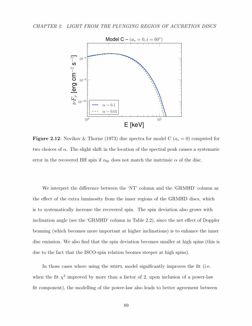
CHAPTER 2. LIGHT FROM THE PLUNGING REGION OF ACCRETION DISCS
Figure 2.12: Novikov & Thorne (1973) disc spectra for model C (a∗ = 0) computed for
two choices of α. The slight shift in the location of the spectral peak causes a systematic
error in the recovered BH spin if αfit does not match the instrinsic α of the disc.
We interpret the difference between the ‘NT’ column and the ‘GRMHD’ column as
the effect of the extra luminosity from the inner regions of the GRMHD discs, which
is to systematically increase the recovered spin. The spin deviation also grows with
inclination angle (see the ‘GRMHD’ column in Table 2.2), since the net effect of Doppler
beaming (which becomes more important at higher inclinations) is to enhance the inner
disc emission. We also find that the spin deviation becomes smaller at high spins (this is
due to the fact that the ISCO-spin relation beomes steeper at high spins).
In those cases where using the simpl model significantly improves the fit (i.e.
when the fit χ2 improved by more than a factor of 2, upon inclusion of a power-law
fit component), the modelling of the power-law also leads to better agreement between
89

CHAPTER 2. LIGHT FROM THE PLUNGING REGION OF ACCRETION DISCS
fitted and input BH spin (compare ‘GRMHD’ and ‘GRMHD+PL’ columns in Table
2.2). By fitting a power-law component, some of the hot photons get associated with the
power-law, which lowers the fitted spin (since the remaining disc spectrum looks softer
after removal of the hard power-law photons). However, we note that the GRMHD
luminosity excess extends even beyond the ISCO (see Fig. 2.1). This explains why even
fitting for the power-law does not completely eliminate the upwards spin bias (i.e. the
‘GRMHD+PL’ columns still yield spins that are higher than the ‘NT’ column in Table
2.2); although some of the excess luminosity is bound up in the nonthermal plunging
region (which can be excluded by means of power-law fitting), there is still some residual
thermal disc luminosity excess, that acts to bias the GRMHD spin upwards. Overall, the
effect of the extra plunging region light results in ∆a∗ ∼ 0.1, 0.06, 0.03 corresponding to
spins a∗ = 0, 0.7, 0.9 respectively (estimated by comparing the ‘NT’ column with the
‘GRMHD’ column in Table 2.2 for the ∼30 per cent Eddington discs).
These systematic spin errors should be thought of as an upper bound since the discs
that we consider correspond to fairly high accretion rates (with L/LEdd > 0.3). Previous
work (Paczynski 2000; Shafee et al. 2008a) suggests that thinner discs (corresponding to
lower accretion rates) better match the Novikov & Thorne (1973) model. Our results in
Table 2.2 also support this claim; in comparing the spin fits from model C (thin disc)
with models D and E (thick discs), we find that model C agrees best to the NT disc
(i.e. that model C has the smallest difference between the ‘NT’ and ‘GRMHD’ columns).
In addition, model C also exhibits the least deviation from a thermal spectrum at high
energies (compare the > 20 keV emission from model C with those of D and E in Fig.
2.9).
We did not simulate lower accretion rate discs due to the rapidly increasing
90
CHAPTER 2. LIGHT FROM THE PLUNGING REGION OF ACCRETION DISCS
computational cost associated with such simulations. Typically, continuum fitting is not
applied to systems where the accretion rate exceeds 30 per cent Eddington since beyond
this critical point, the continuum fitting method is no longer robust to variations in the
disc accretion rate (see McClintock & Remillard 2006; Steiner et al. 2009b). One possible
explanation is that disc self-shadowing becomes important beyond this critical accretion
rate threshold (Li et al. 2010).
To put into perspective how significant our quoted spin deviations are, we compare
our results to the spin uncertainties from actual continuum fitting exercises in the
literature (See Table 2.3). Since the current observational uncertainties are significantly
larger than the deviations that we find in this work, we conclude that the extra light
from the inner and plunging regions of the disc do not limit our ability to make accurate
spin estimates through the continuum fitting method. The current limiting factors
in measuring BH spin are how accurately one can determine the distance, mass, and
inclination of black hole binary systems.
2.7 Discussion
The disc model that we adopt in this work is not completely self-consistent. The
annuli that we compute using tlusty are assumed to have reached their equilibrium
configuration. However, close to the black hole there is simply insufficient time for the
fluid to reach equilibrium (see Fig. 2.13 for a plot of the various time-scales). In addition,
the GRMHD simulations show that the pressure in the innermost regions of the disc is
magnetically dominated, yet in the tlusty annuli calculations, we completely ignore
magnetic pressure support. Previous work by Davis et al. (2009) suggests that including
91
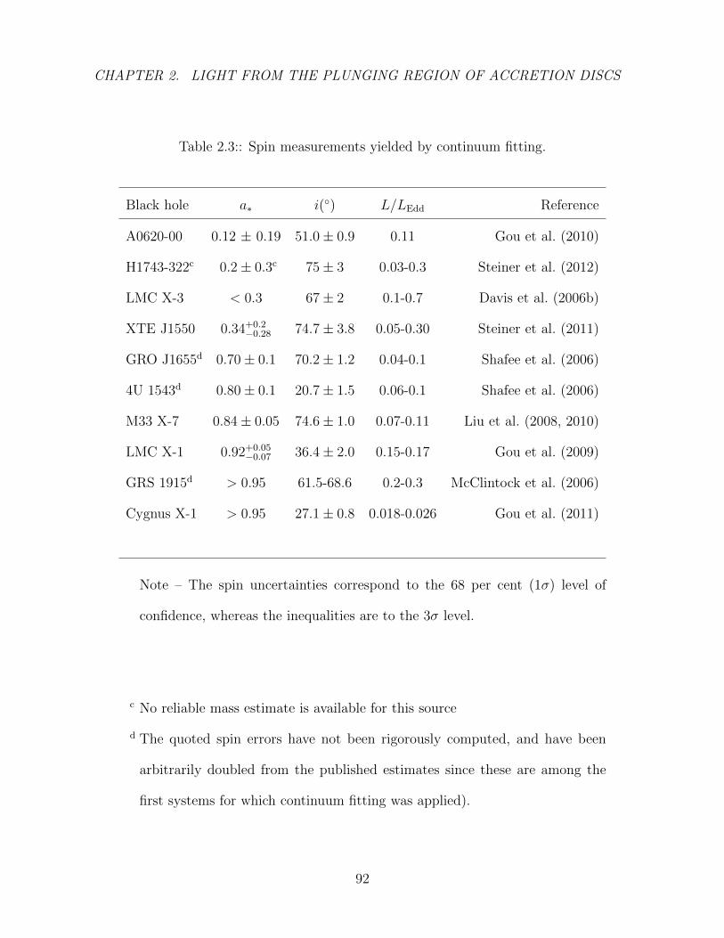
CHAPTER 2. LIGHT FROM THE PLUNGING REGION OF ACCRETION DISCS
Table 2.3:: Spin measurements yielded by continuum fitting.
Black hole a∗ i() L/LEdd Reference
A0620-00 0.12 ± 0.19 51.0± 0.9 0.11 Gou et al. (2010)
H1743-322c 0.2± 0.3c 75± 3 0.03-0.3 Steiner et al. (2012)
LMC X-3 < 0.3 67± 2 0.1-0.7 Davis et al. (2006b)
XTE J1550 0.34+0.2−0.28 74.7± 3.8 0.05-0.30 Steiner et al. (2011)
GRO J1655d 0.70± 0.1 70.2± 1.2 0.04-0.1 Shafee et al. (2006)
4U 1543d 0.80± 0.1 20.7± 1.5 0.06-0.1 Shafee et al. (2006)
M33 X-7 0.84± 0.05 74.6± 1.0 0.07-0.11 Liu et al. (2008, 2010)
LMC X-1 0.92+0.05−0.07 36.4± 2.0 0.15-0.17 Gou et al. (2009)
GRS 1915d > 0.95 61.5-68.6 0.2-0.3 McClintock et al. (2006)
Cygnus X-1 > 0.95 27.1± 0.8 0.018-0.026 Gou et al. (2011)
Note – The spin uncertainties correspond to the 68 per cent (1σ) level of
confidence, whereas the inequalities are to the 3σ level.
c No reliable mass estimate is available for this source
d The quoted spin errors have not been rigorously computed, and have been
arbitrarily doubled from the published estimates since these are among the
first systems for which continuum fitting was applied).
92
CHAPTER 2. LIGHT FROM THE PLUNGING REGION OF ACCRETION DISCS
magnetic support may lead to a slight hardening of the annuli spectrum. Another
problem for the innermost annuli is that they become extremely hot (Tgas > 108 − 109
K), which may invalidate tlusty’s handling of Comptonization (i.e. an angle averaged
Kompaneets treatment, which is only valid for nonrelativistic electrons, see Hubeny et
al. 2001). Finally, due to the increasingly strong light bending effects near the black
hole, the process of disc self-irradiation (i.e. where one part of the disc shines on another
part) may also become important, especially for the innermost annuli (Li et al. 2005).
The net effect of this disc self-irradiation would be to further heat up the annuli, causing
additional spectral hardening. We have ignored disc self-irradiaton in our spectral model
since this reprocessing of light cannot be easily handled by our grid of precomputed
annuli.
These issues primarily affect annuli that are very close to the black hole, which
radiate in the hard X-rays (> 20 keV). We do not expect these inconsistent annuli to
affect our spin fitting results in Table 2.2 since the recovered spin is mainly constrained
by photons near the peak of the spectrum (located at a few keV in Figure 2.9). The
inconsistent annuli will however affect the high energy part of the spectrum, which is
why we caution against reading too deeply into the quantitative details of the power
laws.
93

CHAPTER 2. LIGHT FROM THE PLUNGING REGION OF ACCRETION DISCS
Figure 2.13: Several time-scales of interest are plotted here for model B (a∗ = 0.7). We
show the accretion time-scale (solid blue), the photon diffusion time-scale (dash-dotted
green), the photon absorption time-scale (dotted red), and the photon scattering time-
scale (dashed dark cyan). The absorption and scattering time-scales are computed via
t = 1/(ρκc), using midplane gas densities (ρ) and opacities (κ). The diffusion time-scale is
computed via td = τ 2scattscat where τscat is the scattering optical depth to the disc midplane
(i.e. we expect τ 2scat scatterings to occur before a photon can diffuse out). Note that close
to the black hole, the accretion time-scale becomes shorter than the photon absorption
time-scale, which indicates that the fluid close to the black hole has insufficient time to
reach thermal equilibrium.
94
CHAPTER 2. LIGHT FROM THE PLUNGING REGION OF ACCRETION DISCS
2.7.1 Other signatures of the plunging region
Observations of disc variability could potentially be used to discriminate between our
plunging region model and other coronal models. Assuming that the variability is
caused by Doppler beaming of hotspots moving about in the disc flow, we associate the
hotspot orbital time-scale with the variability time-scale. Since the orbital time decreases
monotonically as one approaches the horizon, the variability from the inner plunging
region of the disc ought to be more rapid than that occurring farther out in disc. Hence,
our plunging region model predicts that the hard X-ray light (originating from the
innermost regions of the disc) would have faster variability than the soft X-ray light
(produced farther out in the thermal disc). Furthermore, in the power-density spectrum
in the hard X-ray bands, we expect most of the variability power to occur above the
ISCO orbital frequency (since we associate this hard emission with the plunging region).
Polarization observations could also serve as a means to distinguish between coronal
models and our plunging region model. Generally, one expects evolution of the polarized
fraction and net polarization angle as the observed photon energy is varied. This is
due to higher energy photons (which are typically emitted closer to the black hole)
feeling stronger relativistic effects, leading to a stronger shift in their polarization
vectors (Schnittman & Krolik 2009, 2010). The planar geometry of the plunging region
may lead to a polarization signature that differs significantly from coronal models.
If the high energy power-law originates from the plunging region, we expect that its
polarization properties will vary continuously from the thermal component to the
non-thermal power-law. This contrasts with some alternative coronal geometries (e.g.
spherical models) that provide abrupt transitions in the polarization properties from
95
CHAPTER 2. LIGHT FROM THE PLUNGING REGION OF ACCRETION DISCS
one component to the next (Schnittman & Krolik 2010). In the plunging region model,
even at energies where the power-law dominates, the polarization fraction and angle will
be consistent with thermal state polarization models that assume a thin disc geometry
(see Schnittman & Krolik 2009). Due to the complex interplay between relativistic
effects, returning radiation, and viewing geometry, a detailed calculation is required to
confirm the above speculation and discriminate between the models. The impending
launch of NASA’s Gravity and Extreme Magnetism Small Explorer (Swank et al. 2010;
GEMS) mission promises observational constraints that may be capable of discriminating
between such models.
2.7.2 How does our choice of cooling function influence the
results?
A criticism that might be levied against the GRMHD simulations is that our choice of
cooling function (as defined in Eq. 2.1) is arbitrary. We have interpreted this cooling
function as the rate of radiative cooling, despite the fact that the GRMHD simulations
do not inherently model radiation physics.
We would like to test how our choice of cooling function impacts the results of
§2.6. Rather than rerunning the GRMHD simulations with another prescription for
cooling (i.e. by changing the functional form of Eq. 2.1), we use the simulation’s
dissipative heating profile as another means to get a cooling rate. Instead of simply
assuming that dissipation equals cooling locally, we consider the physics of energy
advection (i.e. that the fluid releases its heat downstream). To generate a disc model
that is more self-consistent with the TLUSTY annuli, we use the TLUSTY vertical
96
CHAPTER 2. LIGHT FROM THE PLUNGING REGION OF ACCRETION DISCS
structure when computing the rate of energy advection (see Appendix 2.12 for a thorough
exposition on this method of computing the new GRMHD luminosity profile). The new
dissipation-based cooling function (which we label as GRMHD2) releases slightly more
luminosity inside the plunging region (compare the solid and dashed lines in Figure 2.1).
We repeat the same exercise as in §2.6 with this new GRMHD2 derived luminosity
profile. The spectra corresponding to GRMHD2 are shown as the dashed lines in Figure
2.9. Without fitting for the power laws, we find that the recovered spins are slightly
higher owing to the extra plunging region luminosity (compare the ‘GRMHD’ and
‘GRMHD2’ columns in Table 2.2). However, the more realistic fit (i.e. including the
power-law component) takes care of this extra light, yielding comparable spins estimates
to before. The enhanced power laws are purely due to the extra plunging region
luminosity (compare solid and dashed lines in Figures 2.1 and 2.9). The worst cases for
the 30 per cent Eddington discs now have ∆a∗ ∼0.15, 0.07, 0.03, for a∗ = 0, 0.7, 0.9
respectively. Given these results, we still conclude that the extra luminosity from the
GRMHD inner disc does not limit our ability to measure BH spin through the continuum
fitting method (the dominant source of uncertainty is still the observational uncertainties
in distance, mass, and inclination).
As in Kulkarni et al. (2011), we estimate that ∆a∗ ≤ 0.15, which is lower than the
estimate of Noble et al. (2011), who infer ∆a ∼ 0.2 − 0.3 for a Schwarzschild black
hole. Due to the reduced sensitivity of the continuum fitting method at low spins, this
amounts to a somewhat modest discrepancy, which we attribute to various differences
in the setup and intitial conditions of the GRMHD simulations used by the different
groups. We refer the reader to Penna et al. (2010); Kulkarni et al. (2011); Noble et al.
(2010, 2011); Hawley, Guan, & Krolik (2011) for further discussion.
97
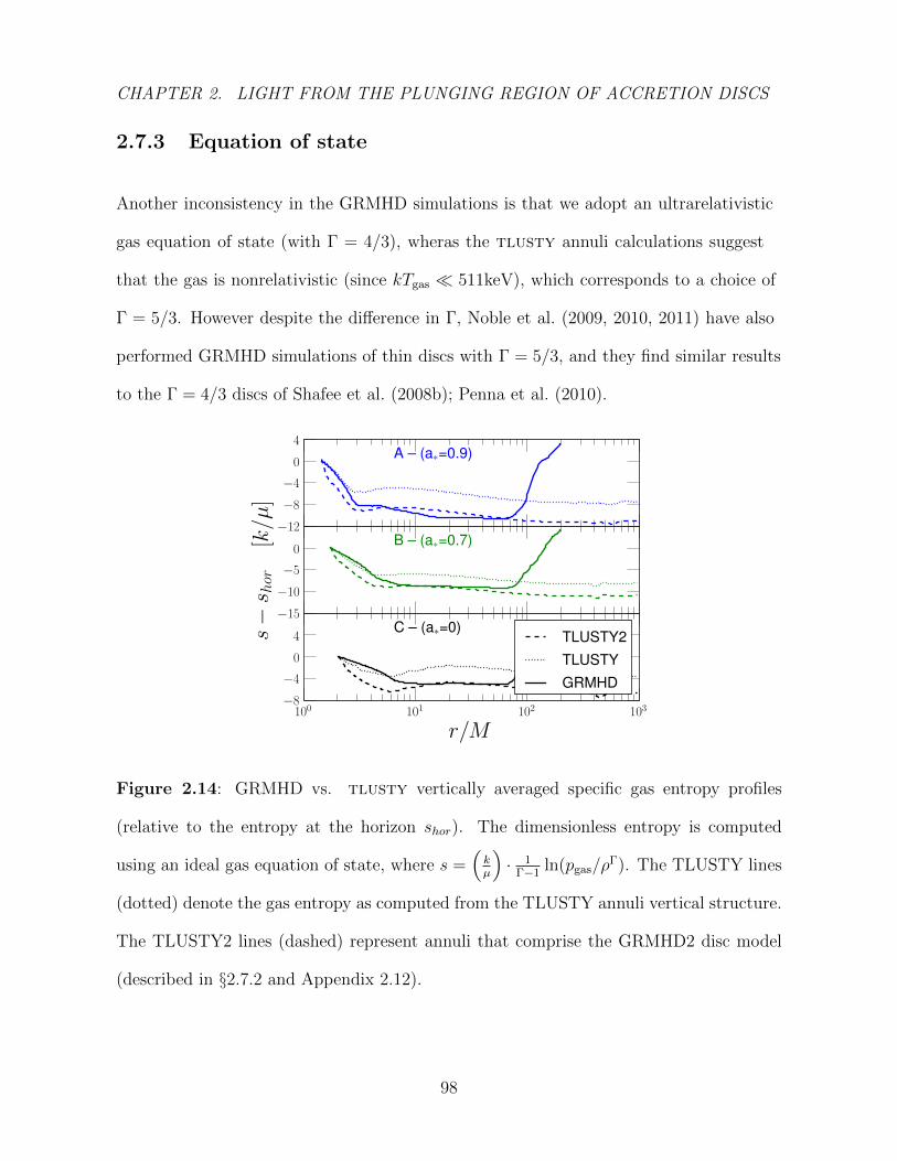
CHAPTER 2. LIGHT FROM THE PLUNGING REGION OF ACCRETION DISCS
2.7.3 Equation of state
Another inconsistency in the GRMHD simulations is that we adopt an ultrarelativistic
gas equation of state (with Γ = 4/3), wheras the tlusty annuli calculations suggest
that the gas is nonrelativistic (since kTgas 511keV), which corresponds to a choice of
Γ = 5/3. However despite the difference in Γ, Noble et al. (2009, 2010, 2011) have also
performed GRMHD simulations of thin discs with Γ = 5/3, and they find similar results
to the Γ = 4/3 discs of Shafee et al. (2008b); Penna et al. (2010).
Figure 2.14: GRMHD vs. tlusty vertically averaged specific gas entropy profiles
(relative to the entropy at the horizon shor). The dimensionless entropy is computed
using an ideal gas equation of state, where s =(kµ
)· 1
Γ−1ln(pgas/ρ
Γ). The TLUSTY lines
(dotted) denote the gas entropy as computed from the TLUSTY annuli vertical structure.
The TLUSTY2 lines (dashed) represent annuli that comprise the GRMHD2 disc model
(described in §2.7.2 and Appendix 2.12).
98
CHAPTER 2. LIGHT FROM THE PLUNGING REGION OF ACCRETION DISCS
In figure 2.14, we examine the relative impact that this equation of state
inconsistency has on the disc’s entropy profile. A fully self-consistent model would have
identical GRMHD and tlusty gas entropy profiles. It appears that well outside the
ISCO, the assumption that the gas cools towards a fixed entropy is supported by the
radiative transfer calculations of tlusty (Compare the flat plateaus in Figure 2.14).
However Figure 2.14 shows that the GRMHD (solid) and TLUSTY (dotted) discs reach
different constant entropies. The alternate disc cooling model (dashed) discussed in
§2.7.2 yields annuli which are more self-consistent with the simulation entropy profile
(compare dashed lines and solid lines in Figure 2.14, which now track each other fairly
well outside the ISCO).
2.8 Summary
The primary goal of this work is to determine how important the neglected light from
the plunging region is in the context of BH spin measurements. To answer this question,
we rely on GRMHD disc simulations of Penna et al. (2010), which capture all but the
radiation physics for magnetized flow around a black hole. We seek to convert these
dimensionless simulations into a form that can be directly compared with observations,
namely the accretion discs’ X-ray continuum spectra.
To do this, we apply radiative transfer post-processing on the simulated discs. This
is an advance over previous work on computing GRMHD disc spectra (i.e. Kulkarni et al.
2011), which assumes (modified) blackbody annuli spectra. We slice the GRMHD disc
into many individual annuli, and for each annulus, we apply a 1-dimensional radiative
transfer calculation to solve for its emergent spectrum. We sum up this collection of local
99

CHAPTER 2. LIGHT FROM THE PLUNGING REGION OF ACCRETION DISCS
spectra by means of ray tracing to get the full disc spectrum, which we then compare
with contemporary disc models used to measure black hole spin. The following are the
key results from this work:
(1). The GRMHD based accretion discs have hotter spectra than the standard
Novikov & Thorne (1973) discs. The GRMHD discs produce more luminosity ev-
erywhere, and the contrast becomes most apparent inside the ISCO (see Figure 2.1).
(2). The increased luminosity of the GRMHD discs compared to the classic NT discs
induces a modest systematic bias in the derived spins of these GRMHD discs. For
black holes of spin a∗ = 0, 0.7, 0.9 the spin deviation is ∆a∗ ∼ 0.15, 0.07, 0.03 in
the worst cases (corresponding to inclination angles of 75). We remark that these
errors are still well within other observational uncertainties (i.e. from not precisely
knowing the system’s mass, inclination, and distance – see Table 2.3).
(3). Without needing to invoke an external corona, the GRMHD discs around spinning
black holes exhibit a weak high-energy power-law tail (Fig. 2.9). This power-law
tail arises from the combined emission of the hot plunging region gas. The strength
of this plunging region power-law increases with the system’s inclination angle.
In our spectral modelling approach, we have made many simplifications and
assumptions (see §2.7), some of which may be incorrect close to the black hole horizon.
Due to these problems, we trust the power laws presented here only to a qualitative level
100
CHAPTER 2. LIGHT FROM THE PLUNGING REGION OF ACCRETION DISCS
– we only trust that the plunging region fluid emits at much higher energies than the
disc, which adds a nonthermal component to the overall spectrum at high energies.
2.9 Luminosity Matching Model
The functional form of the matching flux profile is given below (see Kulkarni et al. 2011,
Page & Thorne 1974 – hereafter PT):
f(r) = fPT(r)− [(E† − ΩL†)2/Ω,r]rie[(E† − ΩL†)2/Ω,r]r
fPT(rie)
−[
Ω,r
(E† − ΩL†)2
]r
C, when r > rie (2.11)
where f(r) = 4πrFcom(r)/M is the dimensionless flux, L†, E†, Ω are the specific angular
momentum, energy-at-infinity, angular velocity (given by Eqs. 15f-h of PT), fPT is the
flux from the Page & Thorne model (Eq. 15n of PT), and C is a free parameter that is
determined by the torque at the inner disc boundary.
The task now is to find an appropriate value of C such that the GRMHD flux and
Eq. 2.11 match at rie. For simplicity, we factor out the radial dependence from the last
two terms of Eq. 2.11 to get:
f(r) = fPT(r)−[
Ω,r
(E† − ΩL†)2
]r
K, (2.12)
where K ≡
[(E† − ΩL†)2/Ω,r]riefPT(rie)− C
is just another constant. To ensure
continuity in the flux profile at rie, we require K to be:
K =
[(E† − ΩL†)2
Ω,r
]rie
[fGRMHD(rie)− fPT(rie)] . (2.13)
101
CHAPTER 2. LIGHT FROM THE PLUNGING REGION OF ACCRETION DISCS
Thus, our final matched flux profile is given by:
σSBTeff(r)4 =
1
−4πrut
dLBL(r)
dr, r ≤ rie, (2.14a)
M
4πrf(r), r > rie, (2.14b)
where LBL(r) is the Boyer-Lindquist luminosity profile measured from the GRMHD
simulations, and f(r) is the dimensionless flux as shown in Eq. 2.12.
2.10 Generalized Novikov & Thorne Model
To get the generalized Novikov & Thorne (1973) column density and radial velocity
profile far out in the disc (to extend the GRMHD simulated disc beyond rie), we solve
the following set of vertical structure equations (with a one-zone model for the vertical
structure):
1. Vertical Pressure Balance:
dPtot
dz= ρg⊥,
has the vertically integrated form of:
Ptot
h= ρQh, (2.15a)
where h is the vertical scale height, and Q = g⊥/z is the prescription for the local
vertical gravity (as defined in Eq. 2.7).
2. Radiative Transfer:
102
CHAPTER 2. LIGHT FROM THE PLUNGING REGION OF ACCRETION DISCS
From the second moment of radiative transfer equation (see §1.8 of Rybicki &
Lightman 1979):
dPrad
dτ=Frad
c,
we transform the dτ optical depth differential to a column mass differential dm via
dτ = κ · dm, where κ is the Rosseland mean opacity. We integrate the column mass
from the surface to the disc midplane (from m = 0 to m = mtot = Σ/2). We also
assume that the flux profile linearly increases with mass away from the midplane
(i.e. F (m) = Ftot (1−m/mtot) – this linearity assumption is also used in tlusty).
The vertically integrated radiative diffusion equation thus becomes
Prad =aT 4
3=FtotκΣ
4c, (2.15b)
where a is the radiation constant, and T is radiation temperature. Note: The factor
2 discrepancy in Eq. 2.15b compared to the standard prescription for radiative
diffusion stems from the linearity assumption in F (m).
3. Stress:
We adopt an α prescription for the stress where tφr = αptot. Vertical integration
yields
W ≡∫ h
−htφrdz = 2hαPtot. (2.15c)
4. Viscous Heating:
103

CHAPTER 2. LIGHT FROM THE PLUNGING REGION OF ACCRETION DISCS
Through the energy equation for viscous heating, it is possible to link the heating
flux with the vertically integrated stress (c.f. 5.6.7-12 of Novikov & Thorne 1973).
The resulting expression is
Ftot =3
4ΩkRF (r)W, (2.15d)
with the dimensionless relativistic factor RF (r) defined as
RF (r) =1− 2/r∗ + a2
∗/r2∗
1− 3/r∗ + 2a∗/r3/2∗.
5. Equation of State:
We ignore magnetic pressure in this analysis, and adopt an ideal gas equation of
state, yielding
Ptot =ρkBT
µ+aT 4
3, (2.15e)
where µ is the mean particle weight of the fluid.
6. Column Density
In this one-zone model, the column density represents the quantity
Σ =
∫ h
−hρdz = 2hρ. (2.15f)
Our goal is to solve Eqs. 2.15 with unknowns (Ptot, ρ, T,Σ, h), given the values of
(κ, µ, α, Ftot, Q,M, r). After some algebra, we obtain an expression for Σ that solves Eqs.
104

CHAPTER 2. LIGHT FROM THE PLUNGING REGION OF ACCRETION DISCS
2.15. We find Σ by solving for the real root of the following polynomial in x:
(F1)2 −[F1
4F3
]x4 −
[2
(3
8
)1/4
F1F2
]x5
+
[(3
8
)1/2
(F2)2
]x10 = 0, (2.16)
where x = Σ1/4 and the polynomial coefficients F1, F2, F3 depend only on the given
values:
F1 =W
α=
4Ftot
3αRFΩk
, (2.17a)
F2 =
(κFtot
2σSB
)1/4(kBµ
), (2.17b)
F3 =c2Q
κ2F 2tot
. (2.17c)
We then solve Eq. 2.16 at different radii to obtain Σ(r) for (r > rie). We pick
κ = κes = 0.3383 cm2 g−1 and µ = 0.615mH , which corresponds to a fluid composition
of 70 per cent Hydrogen, 30 per cent Helium by mass. Given Σ(r), we get the mass
averaged radial velocity by solving for ur in the mass conservation equation M = 2πrΣur.
2.11 Interpolation Methods
All interpolated quantities are computed by linear interpolation in log space (i.e. for two
variables x, and y, we interpolate linearly on log(x) and log(y)). We have chosen this
interpolation scheme since it can perfectly capture all power-law scalings. For quantities
105
CHAPTER 2. LIGHT FROM THE PLUNGING REGION OF ACCRETION DISCS
obtained by interpolating on tlusty annuli (such as the annuli vertical structure), we
employ trilinear interpolation over the 3 annuli parameters log(Teff), log(Σ), and log(Q)
(i.e. each parameter is linearly interpolated seperately in log space).
The interpolation of spectra Iν is handled by a more complicated method to account
for the shape of the Planck function. For an optically thick medium with scattering, the
resultant spectrum takes on the form of a modified blackbody (c.f. Eq. 2.2). Since the
spectra doesn’t depend very sensitively on Σ, or Q, we apply the log-linear interpolation
discussed above for these two annuli parameters. For Teff , we use a more complicated
interpolation scheme. Rather than follow Davis et al. (2005) (they applied a linear
interpolation on the brightness temperature, computed with a fixed spectral hardening
factor of f = 2.0), we switch between three different interpolation methods that each
work for all choices of f . The three methods are applied to different frequency ranges of
the spectrum.
• Method 1: At low frequencies, we have that Iv ∝ Teff in the Raleigh-Jeans tail, and
thus we can apply the linear interpolation method.
• Method 2: At high frequencies, we apply linear interpolation on 1/Teff and log(Iν).
The motivation is that for a blackbody-like spectrum in the high-frequency Wien
limit, the specific intensity as a function of temperature scales as log(Iv) ∝ −1/Teff .
• Method 3: For intermediate frequencies, we take a non-linear combination of the
two interpolation results so that the transition between interpolation methods is
smooth.
106

CHAPTER 2. LIGHT FROM THE PLUNGING REGION OF ACCRETION DISCS
Figure 2.15: Comparison of annuli spectra obtained through the interpolation method
(solid) and an exact calculation (dashed) for the spin a∗ = 0.7 disc. The black spectra
represent annuli outside the plunging region, whereas the red spectrum corresponds to a
plunging region annulus.
Denoting the interpolated intensities using methods 1 and 2 as I1(ν) and I2(ν)
respectively, the expression for the final combined interpolation method is:
Iν(ν) =
I1(ν), ν ≤ ν1,
exp
ln(ν2)− ln(ν)
ln(ν2)− ln(ν1)ln [I1( ν)]
+ln(ν)− ln(ν1)
ln(ν2)− ln(ν1)ln [I2(ν)]
, ν1 < ν < ν2,
I2(ν), ν ≥ ν2.
We have set ν1 = 0.07 νmax, and ν2 = 2.3 νmax, where νmax is the frequency that
maximizes Iν in the spectra of the lowest Teff annuli in the bracketing set used for the
interpolation. These frequency boundary values were determined by minimizing the
107
CHAPTER 2. LIGHT FROM THE PLUNGING REGION OF ACCRETION DISCS
interpolation error for a pure Planck function. For a perfect modified Planck function
with constant f , the chosen ν1 and ν2 correspond to a maximum interpolation error
of 0.08 per cent in Iν for our grid with temperature spacings ∆ log10(Teff) = 0.1. In
practice, the interpolation error after interpolating over the 3 annuli parameters and
emission angle is ∼1 per cent (see Fig. 2.15), except for annuli in the plunging region,
where the flux error grows to ∼10 per cent (the assumption of a constant f is violated
for annuli in the plunging region). The main advantage of this interpolation method is
it provides interpolated spectra that peak very close to the correct frequencies, and the
method works equally well for spectra of all spectral hardening factors.
2.12 An Alternative GRMHD Luminosity Profile
We wish to generate a disc luminosity profile that has the following desirable properties:
1) it is based on the GRMHD dissipation profile rather than cooling profile, and 2) it
produces a disc whose entropy profile is self-consistent with the TLUSTY annuli. We
accomplish this task by considering the physics of energy advection. The idea is to
solve for the radiative cooling rate, taking into account both the dissipative heating rate
(measured from the GRMHD simulations) and the heat advection rate (computed using
the vertical structure from TLUSTY annuli). The energy balance equation relating
these three quantities is:
qadv = qheat − qcool, (2.19)
where qadv is the advected heating rate per unit volume, qheat the viscous heating rate per
unit volume, and qcool is the cooling rate per unit volume (assumed to be purely radiative
108
CHAPTER 2. LIGHT FROM THE PLUNGING REGION OF ACCRETION DISCS
– i.e. we ignore conduction and convection). We take the convention that all hatted
quantities are measured in the comoving frame of the fluid. The advective heating rate is
obtained by evaluating qadv = ρT (ds/dτ), where ρ is the rest mass density, T is the gas
temperature, s is the specific gas entropy of the fluid, and τ is the fluid’s proper time.
Making the approximation that we have stationary axisymmetric flow that is devoid
of motion perpendicular to the midplane, we have ds/dτ = urds/dr via the chain-rule
(ds/dr and ur are evaluated in BL-coordinates). Vertically integrating Eq. 2.19 while
making use of qadv = ρT ur(ds/dr) yields:
Qadv = Qsimheat − Qcool (2.20)
=
∫ +∞
z=−∞ρT ur
(ds
dr
)dz, (2.21)
where Qadv is the vertically integrated heat advection rate (evaluated with TLUSTY
vertical structure), Qsimheat is the vertically integrated viscous heating rate (measured from
the GRMHD simulated discs), and Qcool is the net radiative cooling flux that escapes.
For simplicity in Eq. 2.21, we adopt the following constant mass-averaged radial velocity:
ur =
∫ πθ=0
ρursim√−gdθ∫ π
θ=0ρ√−gdθ
. (2.22)
where ursim represents the pointwise radial velocities measured from GRMHD simulations.
Our goal is to find the value of Qcool that satisfies Eq. 2.20, given that we can
measure Qsimheat from the simulations and calculate Qadv from Eq. 2.21.
109
CHAPTER 2. LIGHT FROM THE PLUNGING REGION OF ACCRETION DISCS
2.12.1 Obtaining the GRMHD dissipation profile
Unfortunately, the GRMHD simulations that we ran were not set up to directly keep
track of the numerical dissipation Qsimheat(r). Despite this lack of information, we can still
estimate the dissipation indirectly by running the argument in Eq. 2.20 backwards; we
solve for the vertically integrated dissipative heating rate
Qsimheat = Qsim
adv + Qsimcool. (2.23)
The ‘sim’ superscript is used to denote quantities derived solely from the GRMHD
simulations (i.e. these quantities are independent of TLUSTY). Analogous to Eq. 2.21,
the vertically integrated12 GRMHD advective heating rate is obtained by
Qsimadv =
∫ π
θ=0
ρT
(ds
dr
)ur√−gdθ. (2.24)
For simplicity, we first apply azimuthal and time averaging to all simulation quantities
used in Eq. 2.24. Since the GRMHD simulations are dimensionless (k/µ = 1) and employ
an ideal gas equation of state, we have that T = Pgas/ρ, and s = (Γ − 1)−1 ln(Pgas/ρΓ).
The GRMHD cooling flux is simply Qsimcool = Fcom where Fcom is the comoving disc flux,
as given by Eq. 2.4.
2.12.2 Net result of the luminosity calculation
The final goal is to solve for the value of Qcool that satisfies Eq. 2.20. The physical
interpretation of this newly derived Qcool is simply the cooling rate corresponding to a
12To maintain consistency with the simulation cooling flux Qsimcool (as calculated by Eqs. 2.3 and 2.4,
which only considers bound disc fluid), the integral in Eq. 2.24 is also only taken over the bound fluid.
110
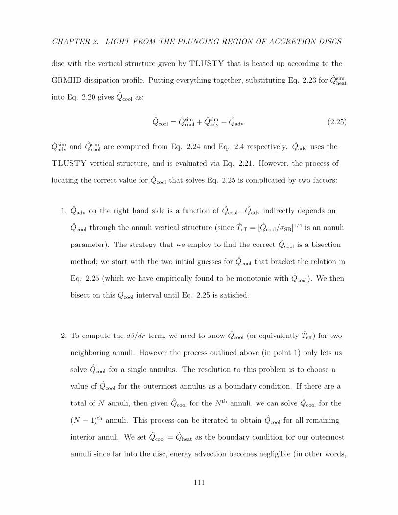
CHAPTER 2. LIGHT FROM THE PLUNGING REGION OF ACCRETION DISCS
disc with the vertical structure given by TLUSTY that is heated up according to the
GRMHD dissipation profile. Putting everything together, substituting Eq. 2.23 for Qsimheat
into Eq. 2.20 gives Qcool as:
Qcool = Qsimcool + Qsim
adv − Qadv. (2.25)
Qsimadv and Qsim
cool are computed from Eq. 2.24 and Eq. 2.4 respectively. Qadv uses the
TLUSTY vertical structure, and is evaluated via Eq. 2.21. However, the process of
locating the correct value for Qcool that solves Eq. 2.25 is complicated by two factors:
1. Qadv on the right hand side is a function of Qcool. Qadv indirectly depends on
Qcool through the annuli vertical structure (since Teff = [Qcool/σSB]1/4 is an annuli
parameter). The strategy that we employ to find the correct Qcool is a bisection
method; we start with the two initial guesses for Qcool that bracket the relation in
Eq. 2.25 (which we have empirically found to be monotonic with Qcool). We then
bisect on this Qcool interval until Eq. 2.25 is satisfied.
2. To compute the ds/dr term, we need to know Qcool (or equivalently Teff) for two
neighboring annuli. However the process outlined above (in point 1) only lets us
solve Qcool for a single annulus. The resolution to this problem is to choose a
value of Qcool for the outermost annulus as a boundary condition. If there are a
total of N annuli, then given Qcool for the N th annuli, we can solve Qcool for the
(N − 1)th annuli. This process can be iterated to obtain Qcool for all remaining
interior annuli. We set Qcool = Qheat as the boundary condition for our outermost
annuli since far into the disc, energy advection becomes negligible (in other words,
111

CHAPTER 2. LIGHT FROM THE PLUNGING REGION OF ACCRETION DISCS
Qadv → 0 far out in the disc, which implies Qcool → Qheat from Eq. 2.20).
Running through the above two steps allows us to solve for Qcool, and hence obtain
a second measure of the disc luminosity (labelled as GRMHD2 in all plots and tables).
Note that the GRMHD2 model is more self-consistent with TLUSTY in Fig. 2.14. The
TLUSTY2 model (computed from the newly derived GRMHD2 disc luminosities) and
the intrinsic GRMHD entropy profiles agree fairly well when r > rISCO.
112

Chapter 3
Thermal Stability in Turbulent
Accretion Discs
This thesis chapter originally appeared in the literature as
Y. Zhu, R. Narayan, MNRAS, 434, 2262, 2013
Abstract
The standard thin accretion disc model predicts that discs around stellar mass black
holes become radiation pressure dominated and thermally unstable once their luminosity
exceeds L & 0.02LEdd. Observationally, discs in the high/soft state of X-ray binaries show
little variability in the range 0.01LEdd < L < 0.5LEdd, implying that these discs in nature
are in fact quite stable. In an attempt to reconcile this conflict, we investigate one-zone
disc models including turbulent and convective modes of vertical energy transport. We
find both mixing mechanisms to have a stabilizing effect, leading to an increase in the
113
CHAPTER 3. CONVECTION AND TURBULENT STABILIZATION OF DISCS
L threshold up to which the disc is thermally stable. In the case of stellar mass black
hole systems, convection alone leads to only a minor increase in this threshold, up to
∼ 5 per cent of Eddington. However turbulent mixing has a much greater effect – the
threshold rises up to 20 per cent Eddington under reasonable assumptions. In optimistic
models with superefficient turbulent mixing, we even find solutions that are completely
thermally stable for all accretion rates. Similar results are obtained for supermassive
black holes, except that all critical accretion rates are a factor ∼10 lower in Eddington
ratio.
3.1 Introduction
Accretion discs are ubiquitous in our universe; their physics governs the production of
powerful jets from Active Galactic Nuclei, the formation of planets, and the growth of
black holes. This wealth of applicability has led to a rich field of study where many open
problems still persist to this day (Frank, King & Raine 2002).
One longstanding puzzle relates to the stability of discs. In the standard α-model
for thin accretion discs (Shakura & Sunyaev 1973; Novikov & Thorne 1973), there
is a critical accretion rate above which the disc transitions from being gas pressure
dominated to radiation pressure dominated, and simultaneously switches from being
thermally stable to unstable (Shakura & Sunyaev 1976; Piran 1978). The model predicts
that the transition should occur at an accretion rate above a few tenths of a per cent
of Eddington, depending on the mass of the central object. Above this rate, we expect
limit-cycle behaviour due to the onset of both thermal instability (Shakura & Sunyaev
1976; Honma, Matsumoto & Kato 1992; Szuszkiewicz & Miller 1998; Janiuk, Czerny
114
CHAPTER 3. CONVECTION AND TURBULENT STABILIZATION OF DISCS
& Siemiginowska 2002) and viscous instability (Lightman & Eardley 1974). However,
observationally there is little variability and no evidence of a limit-cycle for systems with
substantially larger luminosities than the theoretical limit. Indeed, Gierlinski & Done
(2004) show that discs around stellar mass black holes remain stable up to 50 per cent
Eddington, which conflicts with the prediction of standard thin-disc theory by more than
an order of magnitude.
Over the years, many ideas have been proposed to resolve this inconsistency. Piran
(1978) noted that the prediction of thermal instability hinges crucially on taking the
standard α-viscosity prescription in disc models. Other prescriptions for viscosity, such as
having disc stress scale with gas pressure instead of total pressure, admit solutions that
are thermally stable everywhere (Kato, Fukue & Mineshige 2008). However, shearing
box disc simulations with radiation (Hirose, Blaes & Krolik 2009) demonstrate that the
standard α-prescription, in which the stress scales linearly with the total pressure, is
correct. Thus, we do not have freedom to modify the viscosity prescription.
Other attempts to resolve the stability paradox in the context of the α-viscosity
paradigm include modeling discs with: strong irradiation at the disc surface(Tuchman
et al. 1990); a superefficient corona that rapidly siphons heat from the disc and avoids
instability by keeping the disc cool (Svensson & Zdziarski 1994; Rozanska et al. 1999);
strong magnetic pressure support that dominates the vertical structure at low accretion
rates(Zheng et al. 2011); time lags between the generation of disc stress and pressure
response (Ciesielski et al. 2012) as suggested by numerical simulations (Hirose, Krolik &
Blaes 2009); and finally convection (Milsom, Chen & Taam 1994; Goldman & Wandel
1995).
115
CHAPTER 3. CONVECTION AND TURBULENT STABILIZATION OF DISCS
In early works on convective discs, Bisnovatyi-Kogan & Blinnikov (1977) and
Goldman & Wandel (1995) found convection to be superefficient, dominating over
radiation in the vertical transport of energy. This superefficient convective flux strongly
suppresses the radiative channel, resulting in cooler discs that are completely thermally
stable (Goldman & Wandel 1995). However, other groups who performed more detailed
calculations in which they evaluated the complete vertical structure (Shakura et al. 1978;
Cannizzo 1992; Milsom, Chen & Taam 1994; Heinzeller, Duschl & Mineshige 2009) found
a more modest effect where convection carries no more than ∼ 1/2 of the vertical flux of
energy, and has only a weak effect on the disc’s stability (Cannizzo 1992; Milsom, Chen
& Taam 1994; Sadowski et al. 2011).
These later models still find that convection does provide a stabilizing force that
pushes the instability threshold towards higher accretion rates, but the effect is modest
and falls far short of what is needed to explain observations. In this connection, we note
that turbulent convection alone is too small by a factor of 10-100 (Ruden, Papaloizou
& Lin 1988; Ryu & Goodman 1992; Goldman & Wandel 1995) to produce the viscous
stress present in accretion discs (Pringle & Rees 1972; King, Pringle & Livio 2007).
Disc viscosity is believed to arise from the Magneto-Rotational Instability (MRI;
Balbus & Hawley 1991, 1998). One consequence of MRI turbulence is that it will itself
induce a vertical transfer of energy, in a somewhat analogous fashion as convection.
What effect will this have on the thermal stability of the disc? To date, no analytic
model has been developed that takes into account both convection and turbulence. In
this work we attempt to develop the simplest version of such a model. Based on the
results of Agol et al. (2001), we expect turbulent mixing to have a significant impact on
the disc’s vertical structure and hence also on disc stability. We find that turbulence
116
CHAPTER 3. CONVECTION AND TURBULENT STABILIZATION OF DISCS
indeed acts in a similar way to convection, i.e. turbulent discs are substantially more
resilient to the onset of thermal instability. For reasonable choices of model parameters,
we show that it is possible to push the instability threshold up close to the observational
limits.
The organization of the paper is as follows. In §3.2, we present the governing
equations and details of our turbulent disc model. We then proceed to compute three
types of discs using our model: 1) a classic purely radiative disc, 2) a convective disc,
and 3) a convective plus turbulent disc. In §3.3 we compare the stability properties and
radial structure for these three types of disc. Section 3.4 focuses on the impact of various
assumptions made in our disc model and also briefly compares our work to the results
of numerical simulations. Finally, we conclude in §3.5 with a summary of the important
points.
3.2 Physical model
We wish to build the simplest possible disc model that includes the physics of convection
and turbulent vertical mixing. To this end, we separate the equations describing
the disc’s vertical and radial structure, and model the vertical structure as a single
homogeneous slab (see Fig. 3.1). In essence, our approach is similar to the one-zone
relativistic disc model of Novikov & Thorne (1973), but including the effects of convective
and turbulent mixing.
The primary effect of convection and turbulence is to add a new channel for vertical
energy transport. Since the computation of convective flux requires information about
117
CHAPTER 3. CONVECTION AND TURBULENT STABILIZATION OF DISCS
the vertical gradient of temperature, any convective model must have at least two
vertically separated probe points. For convenience, we choose these two sampling points
to be the disc midplane and the density scale height.
The strategy we employ is to first obtain as a function of radius quantities that are
independent of the vertical disc structure. We then use these quantities as boundary
conditions to uniquely specify the disc vertical structure, and hence solve for the complete
disc model.
3.2.1 Radial structure
Luminosity:
For simplicity, we assume that the advected energy is negligible. This allows us to
calculate the net radiative flux leaving the disc at each radius, given only the black hole
mass M , dimensionless spin a∗ = J/(GM2/c), and mass accretion rate M . We adopt the
prescription of Page & Thorne (1974) for determining the disc’s luminosity profile. In
the subsequent vertical structure equations, we make use of the total emergent disc flux
Ftot = σT 4eff . (3.1)
Vertical gravity:
The tidal vertical gravity in the disc is a function purely of the Kerr metric and the
motion of the disc fluid. For circular orbits, the tidal vertical gravity gz is given by
118

CHAPTER 3. CONVECTION AND TURBULENT STABILIZATION OF DISCS
(Riffert & Herold 1995):
gz ≡ Q · z = (GM/r3)1/2Rz(r) · z, (3.2)
where z is height above the midplane, and Rz(r) is a dimensionless relativistic factor
given by:
Rz(r) =1− 4a∗/r
3/2∗ + 3a2
∗/r2∗
1− 3/r∗ + 2a∗/r3/2∗
. (3.3)
We have defined the dimensionless radius r∗ = r/(GM/c2). Note that the quantity
Q = gz/z is independent of z.
Rotation rate:
For circular motion about a Kerr black hole, the orbital velocity is given by (c.f. Novikov
& Thorne 1973):
Ωk =
(GM
r3
)1/2(
1
1 + a∗/r3/2∗
). (3.4)
3.2.2 Vertical structure
Unknown variables
At every fixed radius of the accretion disc, we wish to solve for the following 8 unknowns
that describe the vertical structure:
• Tmid – Midplane temperature
• Pmid – Midplane pressure (gas+radiation)
119
CHAPTER 3. CONVECTION AND TURBULENT STABILIZATION OF DISCS
• Tscale – Temperature at one scale height
• Pscale – Pressure at one scale height (gas+radiation)
• Σ – Vertical column density
• H – Vertical pressure scale height
• ∇ = d lnT/d lnP of the ambient medium
• ∇e = d lnT/d lnP of a convective element
Equations:
We employ the following 8 equations to solve for the 8 unknowns:
1. Vertical pressure balance This gives
dPtot
dz= ρgz,
which has the vertically integrated form:
Ptot
H= ρQH =
ΣQ
2, (3.5)
where H is the vertical pressure scale height, Q = gz/z is defined by Eq.(3.2), and
we have written the density as ρ = Σ/2H in the spirit of a one-zone model.
2. Viscous heating:
Through the energy equation for viscous heating, it is possible to link the disc flux
Ftot with the vertically integrated stress W (See 5.6.7-12 of Novikov & Thorne
1973). The resulting expression is
Ftot =3
4ΩkRF (r)W, (3.6a)
120
CHAPTER 3. CONVECTION AND TURBULENT STABILIZATION OF DISCS
with the dimensionless relativistic factor RF (r) defined as
RF (r) =1− 2/r∗ + a2
∗/r2∗
1− 3/r∗ + 2a∗/r3/2∗. (3.6b)
Taking the α-prescription for the stress (where tφr = αPtot), we have:
W ≡∫ H
−Htφrdz = 2HαPmid. (3.6c)
3. Midplane equation of state:
We ignore magnetic pressure in this analysis, and adopt an ideal gas plus radiation
equation of state,
Pmid =ρkBTmid
µ+aT 4
mid
3
=ΣkBTmid
2Hµ+aT 4
mid
3, (3.7)
where kB is the Boltzmann constant, and µ is the mean molecular weight of the
fluid (taken to be 0.615mH, which corresponds to ionized gas comprised of 70 per
cent Hydrogen and 30 per cent Helium by mass).
4. Equation of state at a density scale height:
We define the density scale height to be where the density falls to e−1 of its
midplane value. Thus the equation here is:
Pscale =ΣkBTscale
2eHµ+aT 4
scale
3. (3.8)
121
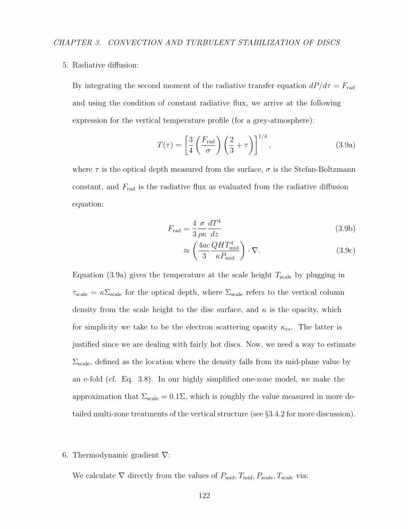
CHAPTER 3. CONVECTION AND TURBULENT STABILIZATION OF DISCS
5. Radiative diffusion:
By integrating the second moment of the radiative transfer equation dP/dτ = Frad
and using the condition of constant radiative flux, we arrive at the following
expression for the vertical temperature profile (for a grey-atmosphere):
T (τ) =
[3
4
(Frad
σ
)(2
3+ τ
)]1/4
, (3.9a)
where τ is the optical depth measured from the surface, σ is the Stefan-Boltzmann
constant, and Frad is the radiative flux as evaluated from the radiative diffusion
equation:
Frad =4
3
σ
ρκ
dT 4
dz(3.9b)
≈(
4ac
3
QHT 4mid
κPmid
)· ∇. (3.9c)
Equation (3.9a) gives the temperature at the scale height Tscale by plugging in
τscale = κΣscale for the optical depth, where Σscale refers to the vertical column
density from the scale height to the disc surface, and κ is the opacity, which
for simplicity we take to be the electron scattering opacity κes. The latter is
justified since we are dealing with fairly hot discs. Now, we need a way to estimate
Σscale, defined as the location where the density falls from its mid-plane value by
an e-fold (cf. Eq. 3.8). In our highly simplified one-zone model, we make the
approximation that Σscale = 0.1Σ, which is roughly the value measured in more de-
tailed multi-zone treatments of the vertical structure (see §3.4.2 for more discussion).
6. Thermodynamic gradient ∇:
We calculate ∇ directly from the values of Pmid, Tmid, Pscale, Tscale via:
122
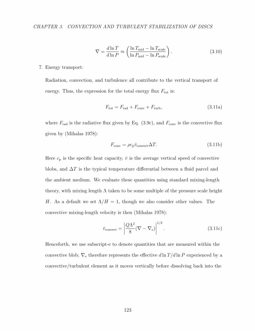
CHAPTER 3. CONVECTION AND TURBULENT STABILIZATION OF DISCS
∇ =d lnT
d lnP≈(
lnTmid − lnTscale
lnPmid − lnPscale
). (3.10)
7. Energy transport:
Radiation, convection, and turbulence all contribute to the vertical transport of
energy. Thus, the expression for the total energy flux Ftot is:
Ftot = Frad + Fconv + Fturb, (3.11a)
where Frad is the radiative flux given by Eq. (3.9c), and Fconv is the convective flux
given by (Mihalas 1978):
Fconv = ρcpvconvect∆T. (3.11b)
Here cp is the specific heat capacity, v is the average vertical speed of convective
blobs, and ∆T is the typical temperature differential between a fluid parcel and
the ambient medium. We evaluate these quantities using standard mixing-length
theory, with mixing length Λ taken to be some multiple of the pressure scale height
H. As a default we set Λ/H = 1, though we also consider other values. The
convective mixing-length velocity is then (Mihalas 1978):
vconvect =
∣∣∣∣QΛ2
8(∇−∇e)
∣∣∣∣1/2 . (3.11c)
Henceforth, we use subscript-e to denote quantities that are measured within the
convective blob; ∇e therefore represents the effective d lnT/d lnP experienced by a
convective/turbulent element as it moves vertically before dissolving back into the
123

CHAPTER 3. CONVECTION AND TURBULENT STABILIZATION OF DISCS
surrounding medium. For the temperature differential, we take:
∆T = Λ
(dT
dz− dT
dz
∣∣∣∣e
)=
ΛT
P
(dp
dz
)(d lnT
d lnP− d lnT
d lnP
∣∣∣∣e
)=
ΛTmid
H(∇−∇e) . (3.11d)
Here, the specific heat capacity cp is given by standard formulae corresponding to a
monatomic gas/radiation mixture (Chandrasekhar 1967) using midplane quantities
to set the gas/radiation pressure ratio.
For turbulent mixing, we follow the same prescription as our convective mixing
length theory (Eq. 3.11b). We assume that the turbulent mixing flux is given by:
Fturb = ρcpvturb∆T (3.11e)
= ρcp(vturbΛturb)Tmid
H(∇−∇e),
where we now invoke a turbulent velocity vturb and turbulent scale height Λturb. To
estimate the size of the product (vturbΛturb), recall that turbulent viscosity has the
form
νturb ∼ vturbΛturb. (3.11f)
Consistency with the α-prescription requires that this viscosity equal
νturb = αcsH, (3.11g)
where α is the viscosity coefficient introduced in Eqs. (3.6), cs =√
2HPmid/Σ
is the fluid sound speed, and H is the disc scale height. Comparing Eqs. 3.11f
and 3.11g and further assuming that Λturb = H, we arrive at vturb = αcs. For the
purpose of exploration, we allow the following more general scaling:
vturb = ζcs, (3.11h)
124
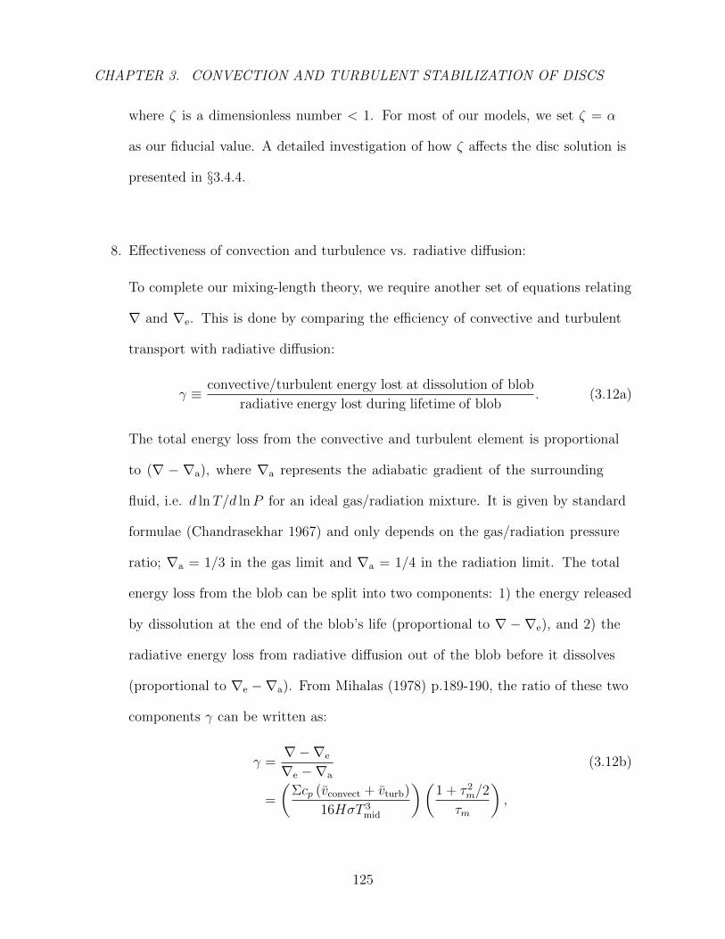
CHAPTER 3. CONVECTION AND TURBULENT STABILIZATION OF DISCS
where ζ is a dimensionless number < 1. For most of our models, we set ζ = α
as our fiducial value. A detailed investigation of how ζ affects the disc solution is
presented in §3.4.4.
8. Effectiveness of convection and turbulence vs. radiative diffusion:
To complete our mixing-length theory, we require another set of equations relating
∇ and ∇e. This is done by comparing the efficiency of convective and turbulent
transport with radiative diffusion:
γ ≡ convective/turbulent energy lost at dissolution of blob
radiative energy lost during lifetime of blob. (3.12a)
The total energy loss from the convective and turbulent element is proportional
to (∇ − ∇a), where ∇a represents the adiabatic gradient of the surrounding
fluid, i.e. d lnT/d lnP for an ideal gas/radiation mixture. It is given by standard
formulae (Chandrasekhar 1967) and only depends on the gas/radiation pressure
ratio; ∇a = 1/3 in the gas limit and ∇a = 1/4 in the radiation limit. The total
energy loss from the blob can be split into two components: 1) the energy released
by dissolution at the end of the blob’s life (proportional to ∇ −∇e), and 2) the
radiative energy loss from radiative diffusion out of the blob before it dissolves
(proportional to ∇e −∇a). From Mihalas (1978) p.189-190, the ratio of these two
components γ can be written as:
γ =∇−∇e
∇e −∇a
(3.12b)
=
(Σcp (vconvect + vturb)
16HσT 3mid
)(1 + τ 2
m/2
τm
),
125
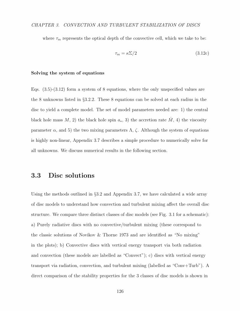
CHAPTER 3. CONVECTION AND TURBULENT STABILIZATION OF DISCS
where τm represents the optical depth of the convective cell, which we take to be:
τm = κΣ/2 (3.12c)
Solving the system of equations
Eqs. (3.5)-(3.12) form a system of 8 equations, where the only unspecified values are
the 8 unknowns listed in §3.2.2. These 8 equations can be solved at each radius in the
disc to yield a complete model. The set of model parameters needed are: 1) the central
black hole mass M , 2) the black hole spin a∗, 3) the accretion rate M , 4) the viscosity
parameter α, and 5) the two mixing parameters Λ, ζ. Although the system of equations
is highly non-linear, Appendix 3.7 describes a simple procedure to numerically solve for
all unknowns. We discuss numerical results in the following section.
3.3 Disc solutions
Using the methods outlined in §3.2 and Appendix 3.7, we have calculated a wide array
of disc models to understand how convection and turbulent mixing affect the overall disc
structure. We compare three distinct classes of disc models (see Fig. 3.1 for a schematic):
a) Purely radiative discs with no convective/turbulent mixing (these correspond to
the classic solutions of Novikov & Thorne 1973 and are identified as “No mixing”
in the plots); b) Convective discs with vertical energy transport via both radiation
and convection (these models are labelled as “Convect”); c) discs with vertical energy
transport via radiation, convection, and turbulent mixing (labelled as “Conv+Turb”). A
direct comparison of the stability properties for the 3 classes of disc models is shown in
126

CHAPTER 3. CONVECTION AND TURBULENT STABILIZATION OF DISCS
Fig. 3.4 and discussed below in §3.3.3. For all cases, we have calculated models spanning
accretion rates over a wide range, 0.001 < M/ ˙MEdd < 1, where we define the Eddington
accretion rate to be:
MEdd =4πGM
κescε. (3.13)
Here ε = 1 − EISCO is the accretion efficiency of the disc, a measure of the total
gravitational energy released by matter along its journey to the ISCO. The efficiency ε
ranges from ∼ 6− 40 per cent depending on black hole spin a∗. Unless specifically noted
otherwise, models were calculated with the following fiducial parameters : black hole
mass M = 10M, black hole spin a∗ = 0, disc radius r∗ = 12 (twice the ISCO radius for
a∗ = 0), viscosity coefficient α = 0.1. For models with convection (models “Convect”
and “Conv+Turb”), the mixing length was set equal to the scale height Λ = H. Finally,
in the case of turbulent mixing (model “Conv+Turb”), the mixing velocity was set to
vturb = αcs, i.e. ζ = α.
127
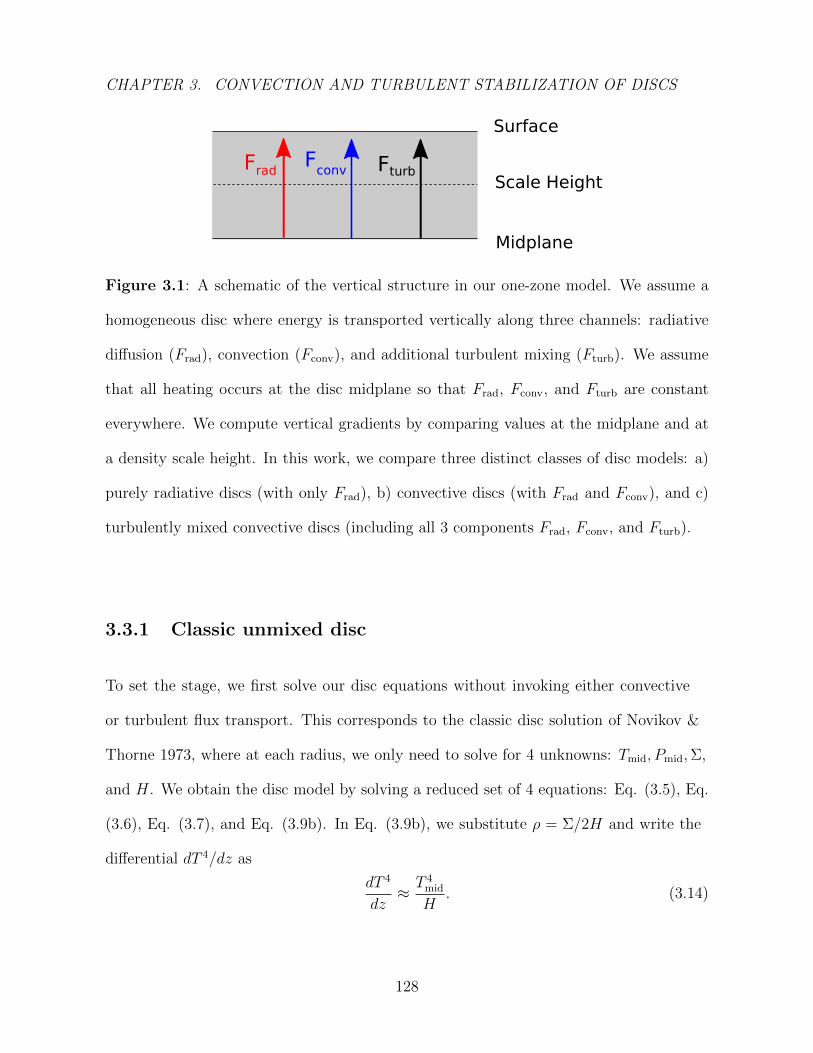
CHAPTER 3. CONVECTION AND TURBULENT STABILIZATION OF DISCS
Figure 3.1: A schematic of the vertical structure in our one-zone model. We assume a
homogeneous disc where energy is transported vertically along three channels: radiative
diffusion (Frad), convection (Fconv), and additional turbulent mixing (Fturb). We assume
that all heating occurs at the disc midplane so that Frad, Fconv, and Fturb are constant
everywhere. We compute vertical gradients by comparing values at the midplane and at
a density scale height. In this work, we compare three distinct classes of disc models: a)
purely radiative discs (with only Frad), b) convective discs (with Frad and Fconv), and c)
turbulently mixed convective discs (including all 3 components Frad, Fconv, and Fturb).
3.3.1 Classic unmixed disc
To set the stage, we first solve our disc equations without invoking either convective
or turbulent flux transport. This corresponds to the classic disc solution of Novikov &
Thorne 1973, where at each radius, we only need to solve for 4 unknowns: Tmid, Pmid,Σ,
and H. We obtain the disc model by solving a reduced set of 4 equations: Eq. (3.5), Eq.
(3.6), Eq. (3.7), and Eq. (3.9b). In Eq. (3.9b), we substitute ρ = Σ/2H and write the
differential dT 4/dz as
dT 4
dz≈ T 4
mid
H. (3.14)
128

CHAPTER 3. CONVECTION AND TURBULENT STABILIZATION OF DISCS
Figure 3.2: Disc solutions in the M − Σ plane (“S-curve”) for a purely radiative disc
with α = 0.1 around a non-spinning black hole. The different tracks represent different
disc radii measured in units of r∗ = r/(GM/c2). The slope dM/dΣ is an indicator
for stability. Solutions with dM/dΣ > 0 are thermally and viscously stable whereas
dM/dΣ < 0 represents instability. Thus, the characteristic bend in the solutions signifies
the transition point from stable to unstable discs. Among the four tracks shown, the
lowest M for the bend occurs at around 2 per cent Eddington in the r∗ = 12 track.
129
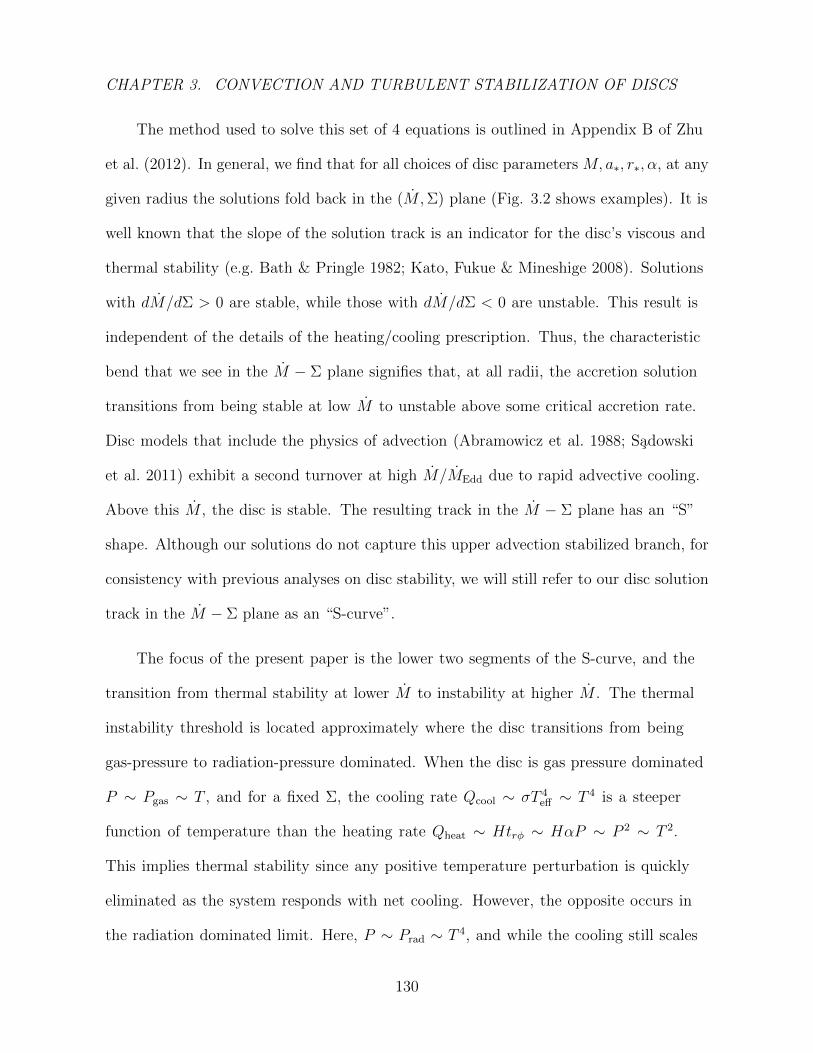
CHAPTER 3. CONVECTION AND TURBULENT STABILIZATION OF DISCS
The method used to solve this set of 4 equations is outlined in Appendix B of Zhu
et al. (2012). In general, we find that for all choices of disc parameters M,a∗, r∗, α, at any
given radius the solutions fold back in the (M,Σ) plane (Fig. 3.2 shows examples). It is
well known that the slope of the solution track is an indicator for the disc’s viscous and
thermal stability (e.g. Bath & Pringle 1982; Kato, Fukue & Mineshige 2008). Solutions
with dM/dΣ > 0 are stable, while those with dM/dΣ < 0 are unstable. This result is
independent of the details of the heating/cooling prescription. Thus, the characteristic
bend that we see in the M − Σ plane signifies that, at all radii, the accretion solution
transitions from being stable at low M to unstable above some critical accretion rate.
Disc models that include the physics of advection (Abramowicz et al. 1988; Sadowski
et al. 2011) exhibit a second turnover at high M/MEdd due to rapid advective cooling.
Above this M , the disc is stable. The resulting track in the M − Σ plane has an “S”
shape. Although our solutions do not capture this upper advection stabilized branch, for
consistency with previous analyses on disc stability, we will still refer to our disc solution
track in the M − Σ plane as an “S-curve”.
The focus of the present paper is the lower two segments of the S-curve, and the
transition from thermal stability at lower M to instability at higher M . The thermal
instability threshold is located approximately where the disc transitions from being
gas-pressure to radiation-pressure dominated. When the disc is gas pressure dominated
P ∼ Pgas ∼ T , and for a fixed Σ, the cooling rate Qcool ∼ σT 4eff ∼ T 4 is a steeper
function of temperature than the heating rate Qheat ∼ Htrφ ∼ HαP ∼ P 2 ∼ T 2.
This implies thermal stability since any positive temperature perturbation is quickly
eliminated as the system responds with net cooling. However, the opposite occurs in
the radiation dominated limit. Here, P ∼ Prad ∼ T 4, and while the cooling still scales
130
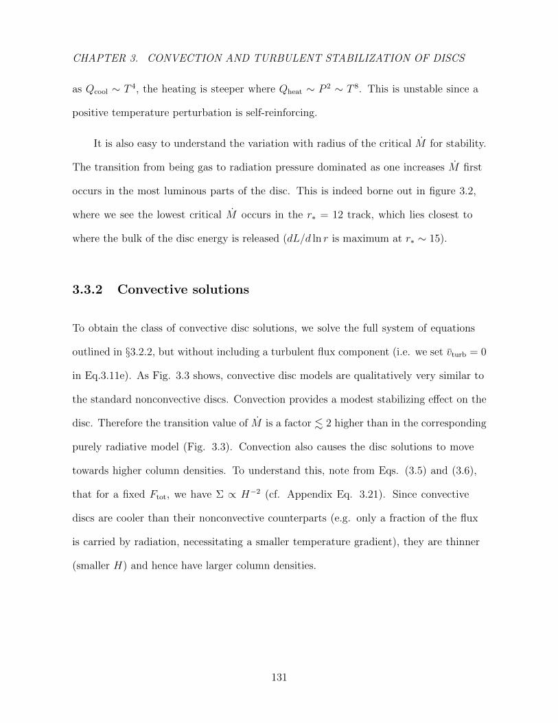
CHAPTER 3. CONVECTION AND TURBULENT STABILIZATION OF DISCS
as Qcool ∼ T 4, the heating is steeper where Qheat ∼ P 2 ∼ T 8. This is unstable since a
positive temperature perturbation is self-reinforcing.
It is also easy to understand the variation with radius of the critical M for stability.
The transition from being gas to radiation pressure dominated as one increases M first
occurs in the most luminous parts of the disc. This is indeed borne out in figure 3.2,
where we see the lowest critical M occurs in the r∗ = 12 track, which lies closest to
where the bulk of the disc energy is released (dL/d ln r is maximum at r∗ ∼ 15).
3.3.2 Convective solutions
To obtain the class of convective disc solutions, we solve the full system of equations
outlined in §3.2.2, but without including a turbulent flux component (i.e. we set vturb = 0
in Eq.3.11e). As Fig. 3.3 shows, convective disc models are qualitatively very similar to
the standard nonconvective discs. Convection provides a modest stabilizing effect on the
disc. Therefore the transition value of M is a factor . 2 higher than in the corresponding
purely radiative model (Fig. 3.3). Convection also causes the disc solutions to move
towards higher column densities. To understand this, note from Eqs. (3.5) and (3.6),
that for a fixed Ftot, we have Σ ∝ H−2 (cf. Appendix Eq. 3.21). Since convective
discs are cooler than their nonconvective counterparts (e.g. only a fraction of the flux
is carried by radiation, necessitating a smaller temperature gradient), they are thinner
(smaller H) and hence have larger column densities.
131
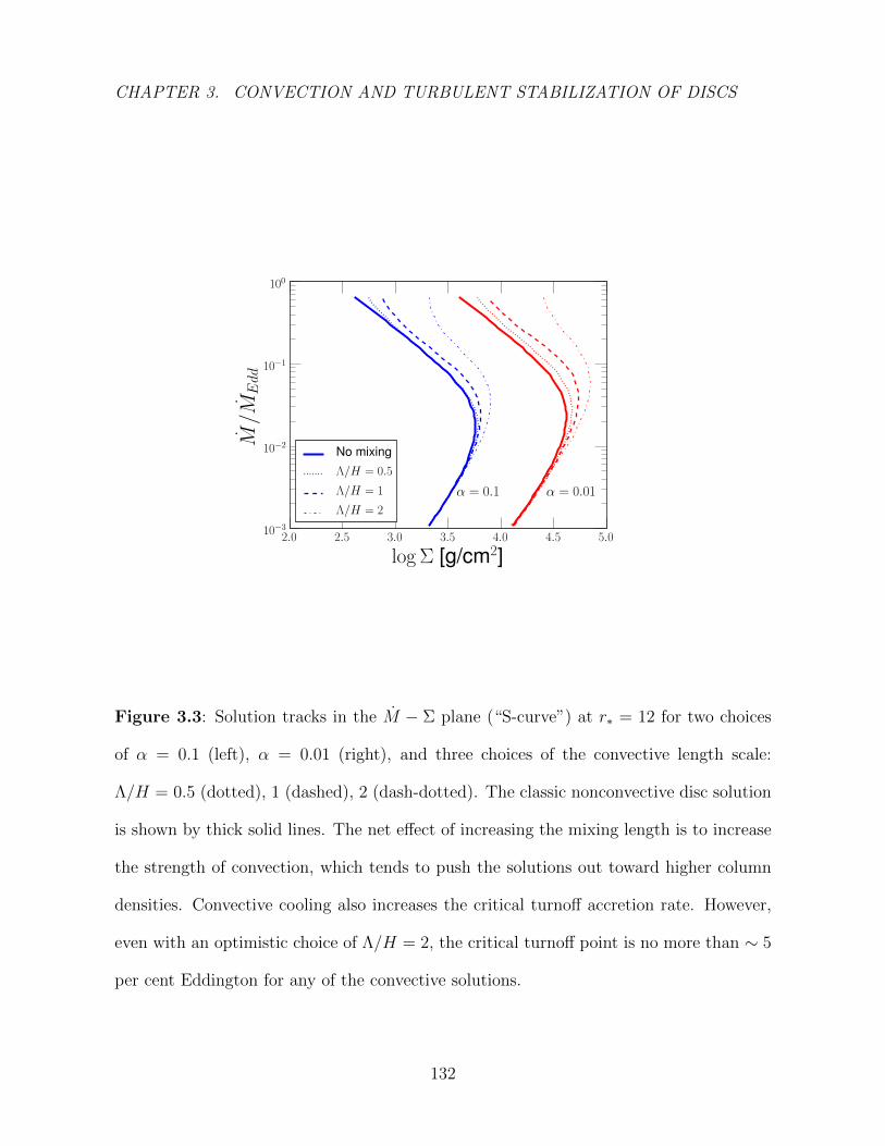
CHAPTER 3. CONVECTION AND TURBULENT STABILIZATION OF DISCS
Figure 3.3: Solution tracks in the M − Σ plane (“S-curve”) at r∗ = 12 for two choices
of α = 0.1 (left), α = 0.01 (right), and three choices of the convective length scale:
Λ/H = 0.5 (dotted), 1 (dashed), 2 (dash-dotted). The classic nonconvective disc solution
is shown by thick solid lines. The net effect of increasing the mixing length is to increase
the strength of convection, which tends to push the solutions out toward higher column
densities. Convective cooling also increases the critical turnoff accretion rate. However,
even with an optimistic choice of Λ/H = 2, the critical turnoff point is no more than ∼ 5
per cent Eddington for any of the convective solutions.
132
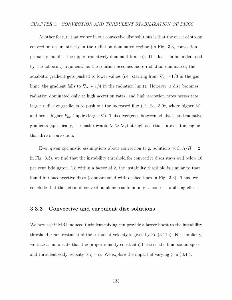
CHAPTER 3. CONVECTION AND TURBULENT STABILIZATION OF DISCS
Another feature that we see in our convective disc solutions is that the onset of strong
convection occurs strictly in the radiation dominated regime (in Fig. 3.3, convection
primarily modifies the upper, radiatively dominant branch). This fact can be understood
by the following argument: as the solution becomes more radiation dominated, the
adiabatic gradient gets pushed to lower values (i.e. starting from ∇a ∼ 1/3 in the gas
limit, the gradient falls to ∇a ∼ 1/4 in the radiation limit). However, a disc becomes
radiation dominated only at high accretion rates, and high accretion rates necessitate
larger radiative gradients to push out the increased flux (cf. Eq. 3.9c, where higher M
and hence higher Frad implies larger ∇). This divergence between adiabatic and radiative
gradients (specifically, the push towards ∇ ∇a) at high accretion rates is the engine
that drives convection.
Even given optimistic assumptions about convection (e.g. solutions with Λ/H = 2
in Fig. 3.3), we find that the instability threshold for convective discs stays well below 10
per cent Eddington. To within a factor of 2, the instability threshold is similar to that
found in nonconvective discs (compare solid with dashed lines in Fig. 3.3). Thus, we
conclude that the action of convection alone results in only a modest stabilizing effect.
3.3.3 Convective and turbulent disc solutions
We now ask if MRI-induced turbulent mixing can provide a larger boost to the instability
threshold. Our treatment of the turbulent velocity is given by Eq.(3.11h). For simplicity,
we take as an ansatz that the proportionality constant ζ between the fluid sound speed
and turbulent eddy velocity is ζ = α. We explore the impact of varying ζ in §3.4.4.
133

CHAPTER 3. CONVECTION AND TURBULENT STABILIZATION OF DISCS
Figure 3.4: S-curves for 3 choices of BH spin, calculated in each case at twice the ISCO
radius: r∗ = (12, 9, 5) for spins a∗ = (0, 0.5, 0.9) respectively. The three sets of curves
correspond to the three classes of disc solutions: classic disc on the left (No mixing),
convective disc in the centre (Convect), and convective + turbulent disc on the right
(Conv+Turb). Varying black hole spin does not have a significant impact on the location
of the turnoff M . Note that the turnoff M in the turbulent models greatly exceed those
in the other two disc models. This shows that the stabilizing effect of turbulent mixing
is much stronger than that of convective mixing alone. The models assume Λ/H = 1,
α = 0.1, and ζ = α.
134
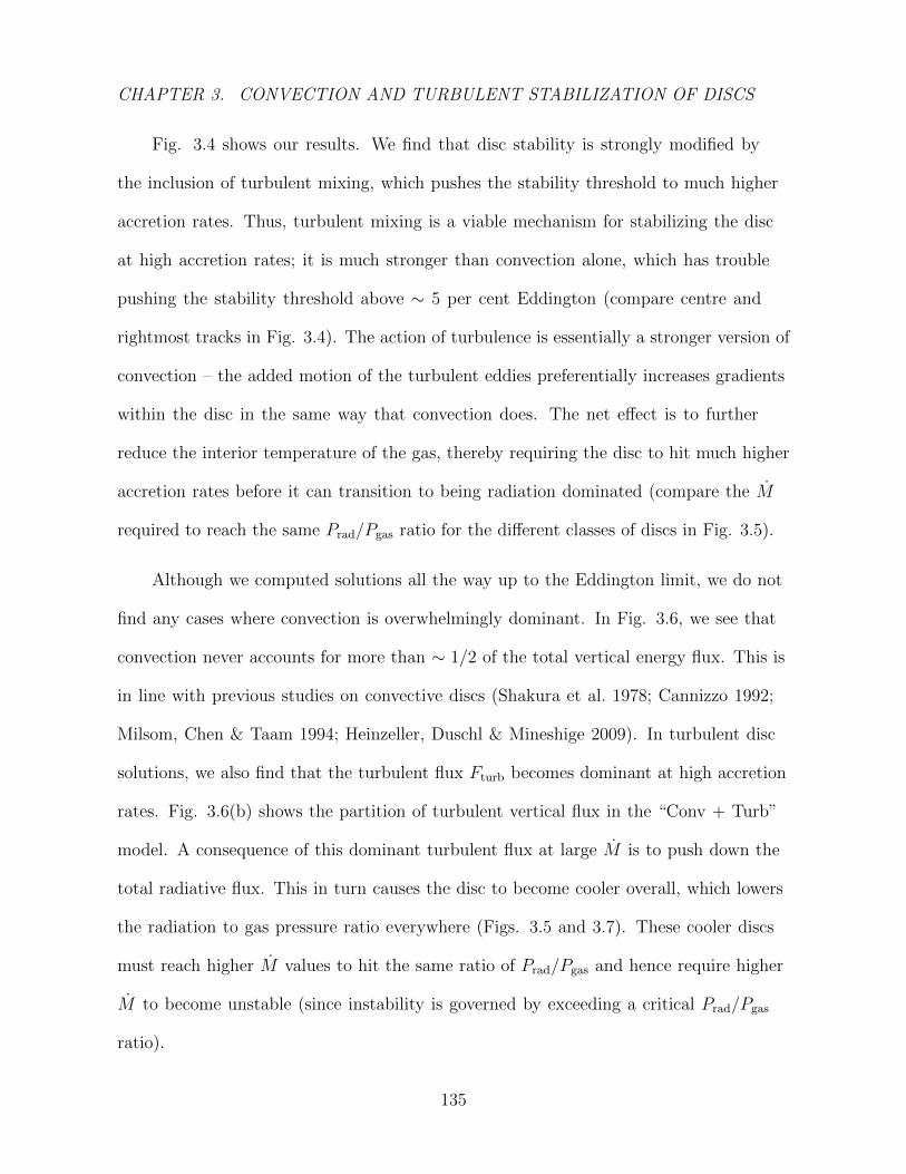
CHAPTER 3. CONVECTION AND TURBULENT STABILIZATION OF DISCS
Fig. 3.4 shows our results. We find that disc stability is strongly modified by
the inclusion of turbulent mixing, which pushes the stability threshold to much higher
accretion rates. Thus, turbulent mixing is a viable mechanism for stabilizing the disc
at high accretion rates; it is much stronger than convection alone, which has trouble
pushing the stability threshold above ∼ 5 per cent Eddington (compare centre and
rightmost tracks in Fig. 3.4). The action of turbulence is essentially a stronger version of
convection – the added motion of the turbulent eddies preferentially increases gradients
within the disc in the same way that convection does. The net effect is to further
reduce the interior temperature of the gas, thereby requiring the disc to hit much higher
accretion rates before it can transition to being radiation dominated (compare the M
required to reach the same Prad/Pgas ratio for the different classes of discs in Fig. 3.5).
Although we computed solutions all the way up to the Eddington limit, we do not
find any cases where convection is overwhelmingly dominant. In Fig. 3.6, we see that
convection never accounts for more than ∼ 1/2 of the total vertical energy flux. This is
in line with previous studies on convective discs (Shakura et al. 1978; Cannizzo 1992;
Milsom, Chen & Taam 1994; Heinzeller, Duschl & Mineshige 2009). In turbulent disc
solutions, we also find that the turbulent flux Fturb becomes dominant at high accretion
rates. Fig. 3.6(b) shows the partition of turbulent vertical flux in the “Conv + Turb”
model. A consequence of this dominant turbulent flux at large M is to push down the
total radiative flux. This in turn causes the disc to become cooler overall, which lowers
the radiation to gas pressure ratio everywhere (Figs. 3.5 and 3.7). These cooler discs
must reach higher M values to hit the same ratio of Prad/Pgas and hence require higher
M to become unstable (since instability is governed by exceeding a critical Prad/Pgas
ratio).
135

CHAPTER 3. CONVECTION AND TURBULENT STABILIZATION OF DISCS
In addition, there is a second effect in operation. For the purely radiative standard
disc, the transition to instability happens at Prad/Pgas = 1.5. This is no longer true for
convective/turbulent models. The critical pressure ratio is 2.1 for the convective model
and is as large as 7.3 for the convective and turbulent model (compare black dots in
Fig. 3.5). This is not too surprising since the critical pressure ratio is achieved when the
growth rate for cooling and heating balance (as a function of fluid temperature). When
the convective and turbulent cooling channels are introduced, one must increase the
overall cooling rate of the system to keep the same radiative flux as before. The heating
rate must therefore increase to balance this increase in cooling. The higher heating rate
implies higher temperatures, or higher radiation to gas pressure ratios. Thus, including
non-radiative channels causes the critical Prad/Pgas to increase.
The net result of these two effects is that models with both convection and
turbulence have critical M values well above 10 per cent Eddington. The cooler interior
caused by the suppression of radiative flux, coupled with the increase in the critical
Prad/Pgas ratio, yields a strong stabilizing effect on the disc. In the models shown in Fig.
3.4, the critical M for turbulent models is about a factor of 10 higher than that of the
purely radiative model. As we show in §3.4.2 & §3.4.4, even larger changes are possible
with modest changes to disc parameters.
136

CHAPTER 3. CONVECTION AND TURBULENT STABILIZATION OF DISCS
Figure 3.5: Comparison of radiation-to-gas pressure ratios for a∗ = 0, r∗ = 12, and the
three classes of disc solutions shown in Fig. 3.4. The large black dots denote the critical
accretion rate for each solution. The pressure ratio for this critical point is not the same
in the three classes of discs: Prad/Pgas = (1.5, 2.1, 7.3) for the radiative, convective, and
turbulent disc models respectively. Note also that we require higher M to reach the same
Prad/Pgas in the convective solutions as in the “no mixing” case.
137
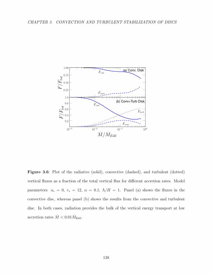
CHAPTER 3. CONVECTION AND TURBULENT STABILIZATION OF DISCS
Figure 3.6: Plot of the radiative (solid), convective (dashed), and turbulent (dotted)
vertical fluxes as a fraction of the total vertical flux for different accretion rates. Model
parameters: a∗ = 0, r∗ = 12, α = 0.1, Λ/H = 1. Panel (a) shows the fluxes in the
convective disc, whereas panel (b) shows the results from the convective and turbulent
disc. In both cases, radiation provides the bulk of the vertical energy transport at low
accretion rates M < 0.01MEdd.
138
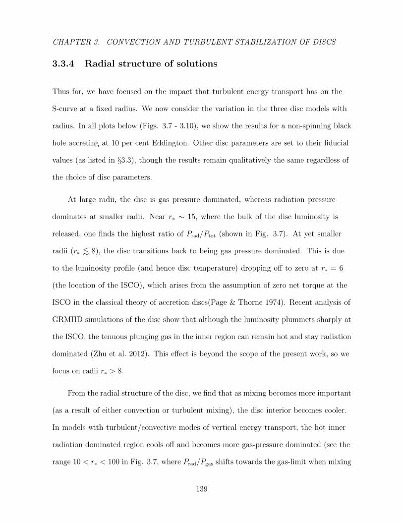
CHAPTER 3. CONVECTION AND TURBULENT STABILIZATION OF DISCS
3.3.4 Radial structure of solutions
Thus far, we have focused on the impact that turbulent energy transport has on the
S-curve at a fixed radius. We now consider the variation in the three disc models with
radius. In all plots below (Figs. 3.7 - 3.10), we show the results for a non-spinning black
hole accreting at 10 per cent Eddington. Other disc parameters are set to their fiducial
values (as listed in §3.3), though the results remain qualitatively the same regardless of
the choice of disc parameters.
At large radii, the disc is gas pressure dominated, whereas radiation pressure
dominates at smaller radii. Near r∗ ∼ 15, where the bulk of the disc luminosity is
released, one finds the highest ratio of Prad/Ptot (shown in Fig. 3.7). At yet smaller
radii (r∗ . 8), the disc transitions back to being gas pressure dominated. This is due
to the luminosity profile (and hence disc temperature) dropping off to zero at r∗ = 6
(the location of the ISCO), which arises from the assumption of zero net torque at the
ISCO in the classical theory of accretion discs(Page & Thorne 1974). Recent analysis of
GRMHD simulations of the disc show that although the luminosity plummets sharply at
the ISCO, the tenuous plunging gas in the inner region can remain hot and stay radiation
dominated (Zhu et al. 2012). This effect is beyond the scope of the present work, so we
focus on radii r∗ > 8.
From the radial structure of the disc, we find that as mixing becomes more important
(as a result of either convection or turbulent mixing), the disc interior becomes cooler.
In models with turbulent/convective modes of vertical energy transport, the hot inner
radiation dominated region cools off and becomes more gas-pressure dominated (see the
range 10 < r∗ < 100 in Fig. 3.7, where Prad/Pgas shifts towards the gas-limit when mixing
139
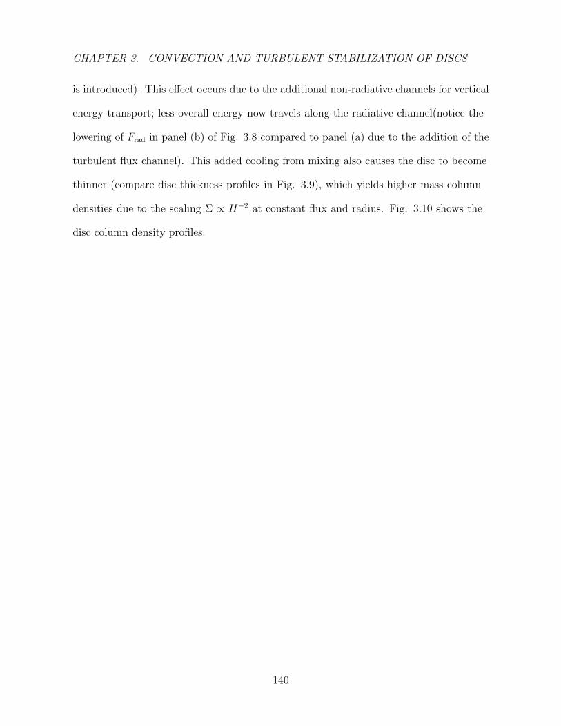
CHAPTER 3. CONVECTION AND TURBULENT STABILIZATION OF DISCS
is introduced). This effect occurs due to the additional non-radiative channels for vertical
energy transport; less overall energy now travels along the radiative channel(notice the
lowering of Frad in panel (b) of Fig. 3.8 compared to panel (a) due to the addition of the
turbulent flux channel). This added cooling from mixing also causes the disc to become
thinner (compare disc thickness profiles in Fig. 3.9), which yields higher mass column
densities due to the scaling Σ ∝ H−2 at constant flux and radius. Fig. 3.10 shows the
disc column density profiles.
140
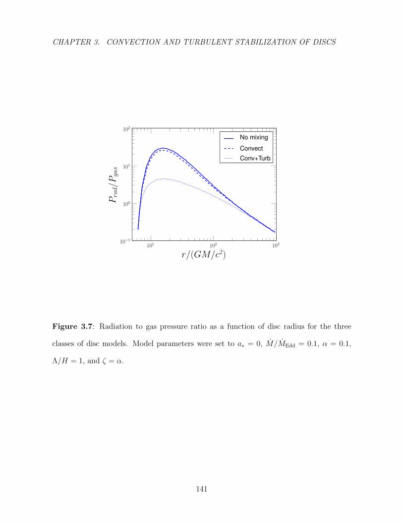
CHAPTER 3. CONVECTION AND TURBULENT STABILIZATION OF DISCS
Figure 3.7: Radiation to gas pressure ratio as a function of disc radius for the three
classes of disc models. Model parameters were set to a∗ = 0, M/MEdd = 0.1, α = 0.1,
Λ/H = 1, and ζ = α.
141

CHAPTER 3. CONVECTION AND TURBULENT STABILIZATION OF DISCS
Figure 3.8: Radial dependence of the fractional vertical fluxes in the radiative (solid),
convective (dashed), and turbulent (dotted) channels for 10 per cent Eddington solutions.
The upper panel (a) corresponds to the purely convective case, and the lower panel (b)
corresponds to the turbulent plus convective case. Note that the convective flux saturates
at about ∼ 1/5 of the total flux. Model parameters are the same as in Fig. 3.7.
142
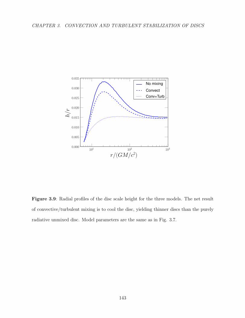
CHAPTER 3. CONVECTION AND TURBULENT STABILIZATION OF DISCS
Figure 3.9: Radial profiles of the disc scale height for the three models. The net result
of convective/turbulent mixing is to cool the disc, yielding thinner discs than the purely
radiative unmixed disc. Model parameters are the same as in Fig. 3.7.
143
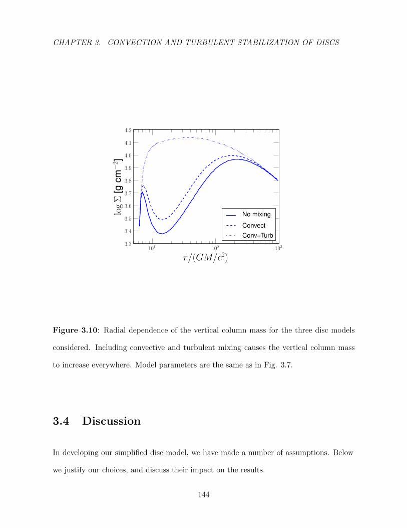
CHAPTER 3. CONVECTION AND TURBULENT STABILIZATION OF DISCS
Figure 3.10: Radial dependence of the vertical column mass for the three disc models
considered. Including convective and turbulent mixing causes the vertical column mass
to increase everywhere. Model parameters are the same as in Fig. 3.7.
3.4 Discussion
In developing our simplified disc model, we have made a number of assumptions. Below
we justify our choices, and discuss their impact on the results.
144
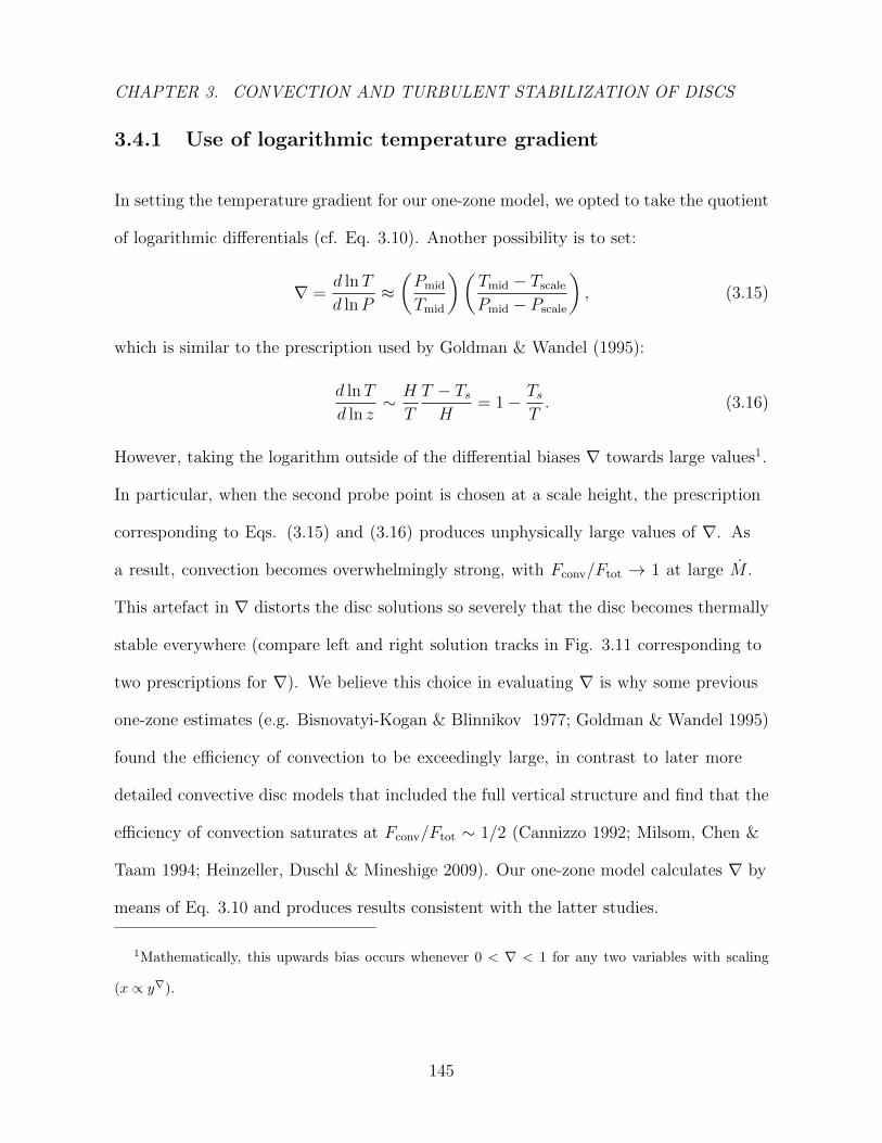
CHAPTER 3. CONVECTION AND TURBULENT STABILIZATION OF DISCS
3.4.1 Use of logarithmic temperature gradient
In setting the temperature gradient for our one-zone model, we opted to take the quotient
of logarithmic differentials (cf. Eq. 3.10). Another possibility is to set:
∇ =d lnT
d lnP≈(Pmid
Tmid
)(Tmid − Tscale
Pmid − Pscale
), (3.15)
which is similar to the prescription used by Goldman & Wandel (1995):
d lnT
d ln z∼ H
T
T − TsH
= 1− TsT. (3.16)
However, taking the logarithm outside of the differential biases ∇ towards large values1.
In particular, when the second probe point is chosen at a scale height, the prescription
corresponding to Eqs. (3.15) and (3.16) produces unphysically large values of ∇. As
a result, convection becomes overwhelmingly strong, with Fconv/Ftot → 1 at large M .
This artefact in ∇ distorts the disc solutions so severely that the disc becomes thermally
stable everywhere (compare left and right solution tracks in Fig. 3.11 corresponding to
two prescriptions for ∇). We believe this choice in evaluating ∇ is why some previous
one-zone estimates (e.g. Bisnovatyi-Kogan & Blinnikov 1977; Goldman & Wandel 1995)
found the efficiency of convection to be exceedingly large, in contrast to later more
detailed convective disc models that included the full vertical structure and find that the
efficiency of convection saturates at Fconv/Ftot ∼ 1/2 (Cannizzo 1992; Milsom, Chen &
Taam 1994; Heinzeller, Duschl & Mineshige 2009). Our one-zone model calculates ∇ by
means of Eq. 3.10 and produces results consistent with the latter studies.
1Mathematically, this upwards bias occurs whenever 0 < ∇ < 1 for any two variables with scaling
(x ∝ y∇).
145
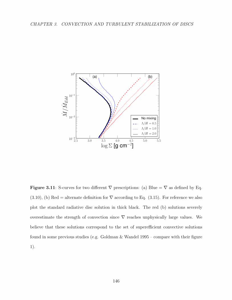
CHAPTER 3. CONVECTION AND TURBULENT STABILIZATION OF DISCS
Figure 3.11: S-curves for two different ∇ prescriptions: (a) Blue = ∇ as defined by Eq.
(3.10), (b) Red = alternate definition for ∇ according to Eq. (3.15). For reference we also
plot the standard radiative disc solution in thick black. The red (b) solutions severely
overestimate the strength of convection since ∇ reaches unphysically large values. We
believe that these solutions correspond to the set of superefficient convective solutions
found in some previous studies (e.g. Goldman & Wandel 1995 – compare with their figure
1).
146
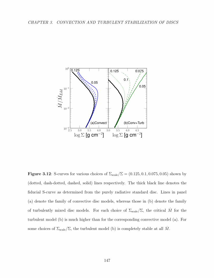
CHAPTER 3. CONVECTION AND TURBULENT STABILIZATION OF DISCS
Figure 3.12: S-curves for various choices of Σscale/Σ = (0.125, 0.1, 0.075, 0.05) shown by
(dotted, dash-dotted, dashed, solid) lines respectively. The thick black line denotes the
fiducial S-curve as determined from the purely radiative standard disc. Lines in panel
(a) denote the family of convective disc models, whereas those in (b) denote the family
of turbulently mixed disc models. For each choice of Σscale/Σ, the critical M for the
turbulent model (b) is much higher than for the corresponding convective model (a). For
some choices of Σscale/Σ, the turbulent model (b) is completely stable at all M .
147

CHAPTER 3. CONVECTION AND TURBULENT STABILIZATION OF DISCS
3.4.2 Impact of Σscale
In our disc model, one arbitrary parameter is the scale height Σscale used as the upper
probe point in defining the temperature gradient ∇. In all models presented so far,
we set Σscale = 0.1Σ. Fig. 3.12 shows the impact of varying Σscale. We find that the
critical M is quite sensitive to the choice of Σscale. In general, larger values of Σscale
act to weaken the strength of mixing, resulting in smaller critical M values. However,
regardless of the value picked for Σscale, the critical M for the turbulently mixed disc is
always much higher than that of the convective disc (compare left and right panels in
Fig. 3.12 for the same choice of Σscale).
We have looked at more detailed treatments of the vertical structure to see how
good our estimate of Σscale is. For the purely radiative standard disc, we have computed
a few detailed models of the vertical structure across a wide range of accretion rates
(from 0.1−50 per cent Eddington) using the stellar atmospheres code TLUSTY (Hubeny
& Lanz 1995; Davis et al. 2005). We find Σscale ∼ 0.03− 0.15Σ, with a systematic trend
such that Σscale/Σ is lower at large M . This is simply a consequence of the disc becoming
more centrally concentrated when it is cool and in the gas-pressure dominated limit.
As another reference point, a polytropic disc with equation of state P = Kρ1+1/n,
where K is a constant and n is the polytropic index, has a density profile given by
ρ(z)
ρ(z = 0)=
(1−
( zH
)2)n
, (3.17)
where z is the height above the midplane, H is the total height of the disc, and ρ0 is
the central density. For n = 3/2 (corresponding to a strongly convective column), we
have Σscale/Σ ∼ 0.04. For n = 3 (corresponding to a radiatively cooled column), we find
Σscale/Σ ∼ 0.06.
148
CHAPTER 3. CONVECTION AND TURBULENT STABILIZATION OF DISCS
For the case of an isothermal disc, the vertical density profile is given by
ρ(z)
ρ(z = 0)= exp
[−z2/2
]. (3.18)
This corresponds to Σscale = erfc(1) · Σ/2 ≈ 0.08Σ. In all cases, the value of Σscale
is pretty close (i.e. within a factor of 2) to the fiducial value that we have adopted
in our models (Σscale ∼ 0.1). If anything, our choice is conservative since values of
(Σscale < 0.1Σ) enhance the stability of these models (Fig. 3.12).
3.4.3 Scaling of Critical M with Black Hole Mass
So far, we have only treated the case where M = 10M. However, from eq. (2.18) of
Shakura & Sunyaev (1973) we expect a weak Mcrit ∝M−1/8 scaling for the critical point
in the S-curve. Figure 3.13 shows the scaling for our disc models. For supermassive black
holes with masses M ∼ 107−8M, we expect a roughly tenfold reduction in the critical
accretion rate threshold compared to stellar mass black holes, and this is seen in the
plot. Convection and turbulence increase Mcrit by the same factor ∼ 10. Even with this,
we see that AGN discs are stable only up to luminosities of ∼ 3 per cent of Eddington.
149
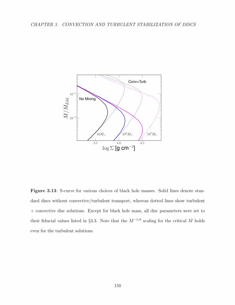
CHAPTER 3. CONVECTION AND TURBULENT STABILIZATION OF DISCS
Figure 3.13: S-curve for various choices of black hole masses. Solid lines denote stan-
dard discs without convective/turbulent transport, whereas dotted lines show turbulent
+ convective disc solutions. Except for black hole mass, all disc parameters were set to
their fiducial values listed in §3.3. Note that the M−1/8 scaling for the critical M holds
even for the turbulent solutions.
150

CHAPTER 3. CONVECTION AND TURBULENT STABILIZATION OF DISCS
3.4.4 Choosing ζ – comparison with simulations
The value that we take for ζ = vturb/cs in our model is primarily motivated by the
speed of turbulent motions observed in numerical simulations. From the global GRMHD
simulations of Penna et al. (2010), we find that vturb/cs ∼ 0.1− 0.2 for r∗ > 10 (compare
dashed and solid lines in Fig. 3.14). The effective viscosity coefficient in these simulations
is measured to be α ∼ 0.05 − 0.1, consistent with our choice ζ = α. However shearing
box simulations measure a much larger spread in the vertical advective speed (see figure
23 in Blaes et al. 2011), which can range from vturb ∼ 0.001− 0.1cs depending sensitively
on where the advective speed is measured (slowest at midplane, faster at surface). Note
that for shearing box simulations, the effective viscosity α is also much lower than the
corresponding values in global simulations; typical values are α ∼ 0.01 (King, Pringle &
Livio 2007). Table 3.1 shows a list of inferred ζ values from various simulations in the
literature, and we find the scaling is roughly ζ ∼ 2α. Note that this scaling for vturb ∝ α
is inconsistent with an isotropically turbulent α-model since the stress would now scale
as W ∝ ρv2 ∝ v2turb ∝ α2 6= α. The only way to reconcile this inconsistency is to demand
anisotropic turbulence so that the scaling of W with v2turb no longer holds.
To test the sensitivity of our model on the choice of turbulent speed, we now explore
a wide range of values for ζ. The precise location of the critical M for stability depends
sensitively on the value of ζ (see the spread of solutions in Figs. 3.15 and 3.16). For
sufficiently large ζ (not much larger than our canonical value of 0.1), the turbulent disc
becomes stable for all accretion rates. Due to sensitivity to model parameters, this
prediction should be treated with caution and must be interpreted more as a proof
of concept. Our main result is that turbulent mixing can provide a much stronger
151

CHAPTER 3. CONVECTION AND TURBULENT STABILIZATION OF DISCS
Table 3.1:: Simulation Derived ζ = vturb/cs Values
Reference α ζ Method
Jiang et al. (2013) 0.01-0.02 0.036 Butterfly1
Guan & Gammie (2011) 0.01-0.02 0.045 Butterfly1
Blaes et al. (2011) 0.01-0.02 0.021 Direct2
Penna et al. (2010) 0.05-0.1 0.1-0.2 Direct2
Davis et al. (2010) ∼0.01 0.026 Butterfly1
Suzuki & Inutsuka (2009) ∼0.01 0.025 Butterfly1
1 Vertical advection speed is measured from the slope of
the simulation butterfly diagram (which shows the char-
acteristic vertical motion of the turbulent dynamo). This
slope yields vturb in terms of HΩ = cs. In cases with non-
constant slope, we use the slope measured at z/H = 1.
2 We compare direct measurements of vturb = vz and cs at
z/H = 1 to get ζ.
152
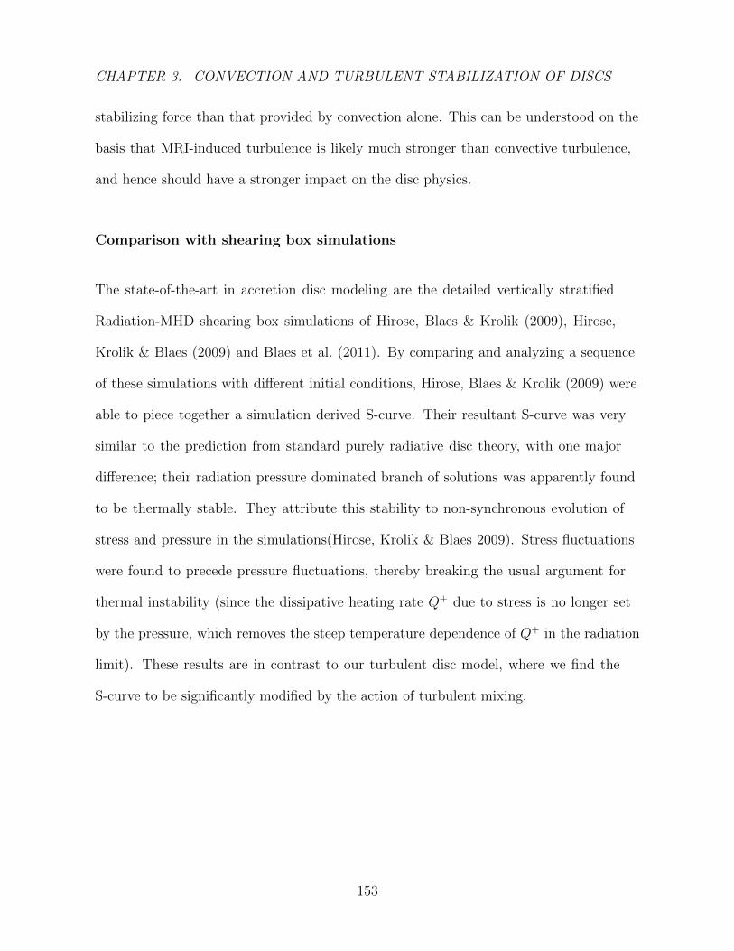
CHAPTER 3. CONVECTION AND TURBULENT STABILIZATION OF DISCS
stabilizing force than that provided by convection alone. This can be understood on the
basis that MRI-induced turbulence is likely much stronger than convective turbulence,
and hence should have a stronger impact on the disc physics.
Comparison with shearing box simulations
The state-of-the-art in accretion disc modeling are the detailed vertically stratified
Radiation-MHD shearing box simulations of Hirose, Blaes & Krolik (2009), Hirose,
Krolik & Blaes (2009) and Blaes et al. (2011). By comparing and analyzing a sequence
of these simulations with different initial conditions, Hirose, Blaes & Krolik (2009) were
able to piece together a simulation derived S-curve. Their resultant S-curve was very
similar to the prediction from standard purely radiative disc theory, with one major
difference; their radiation pressure dominated branch of solutions was apparently found
to be thermally stable. They attribute this stability to non-synchronous evolution of
stress and pressure in the simulations(Hirose, Krolik & Blaes 2009). Stress fluctuations
were found to precede pressure fluctuations, thereby breaking the usual argument for
thermal instability (since the dissipative heating rate Q+ due to stress is no longer set
by the pressure, which removes the steep temperature dependence of Q+ in the radiation
limit). These results are in contrast to our turbulent disc model, where we find the
S-curve to be significantly modified by the action of turbulent mixing.
153

CHAPTER 3. CONVECTION AND TURBULENT STABILIZATION OF DISCS
Figure 3.14: GRMHD derived turbulent vertical velocities for a non-spinning black hole
from run A0HR07 of Penna et al. (2010), in which α = 0.05 − 0.1. The time-averaged
root-mean-squared value of the vertical velocity vz as measured at the disc midplane (blue
solid) and at a scale height (green dotted) are shown and compared to the simulation sound
speed (red dashed). The simulation gives vz/cs ∼ 0.1 far from the plunging region (for
r∗ > 10), corresponding to ζ ≈ 0.1 ≈ α.
154

CHAPTER 3. CONVECTION AND TURBULENT STABILIZATION OF DISCS
Figure 3.15: S-curve for various choices of the turbulent mixing parameter ζ. Model
parameters: α = 0.1, a∗ = 0, r∗ = 12,Λ/H = 1. The red solid track (ζ = 0) represents a
convective disc solution (i.e. no turbulent flux). For small values of ζ ∼ 0.01, turbulence
has negligible impact on the disc solutions. However, for ζ & 0.05, the critical M is
increased substantially, and for ζ > 0.1 the disc is stable for all values of M .
155
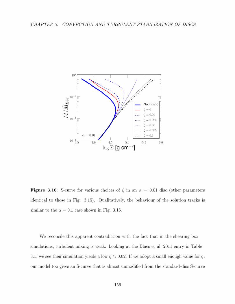
CHAPTER 3. CONVECTION AND TURBULENT STABILIZATION OF DISCS
Figure 3.16: S-curve for various choices of ζ in an α = 0.01 disc (other parameters
identical to those in Fig. 3.15). Qualitatively, the behaviour of the solution tracks is
similar to the α = 0.1 case shown in Fig. 3.15.
We reconcile this apparent contradiction with the fact that in the shearing box
simulations, turbulent mixing is weak. Looking at the Blaes et al. 2011 entry in Table
3.1, we see their simulation yields a low ζ ≈ 0.02. If we adopt a small enough value for ζ,
our model too gives an S-curve that is almost unmodified from the standard-disc S-curve
156
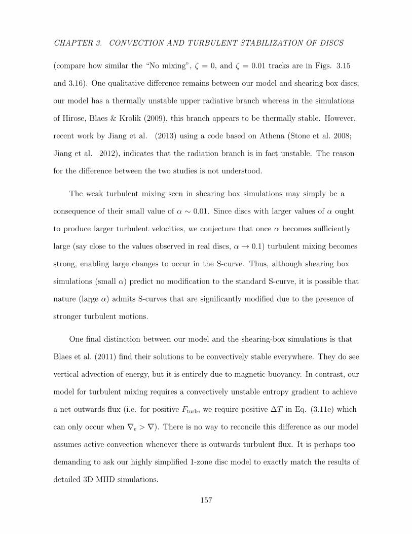
CHAPTER 3. CONVECTION AND TURBULENT STABILIZATION OF DISCS
(compare how similar the “No mixing”, ζ = 0, and ζ = 0.01 tracks are in Figs. 3.15
and 3.16). One qualitative difference remains between our model and shearing box discs;
our model has a thermally unstable upper radiative branch whereas in the simulations
of Hirose, Blaes & Krolik (2009), this branch appears to be thermally stable. However,
recent work by Jiang et al. (2013) using a code based on Athena (Stone et al. 2008;
Jiang et al. 2012), indicates that the radiation branch is in fact unstable. The reason
for the difference between the two studies is not understood.
The weak turbulent mixing seen in shearing box simulations may simply be a
consequence of their small value of α ∼ 0.01. Since discs with larger values of α ought
to produce larger turbulent velocities, we conjecture that once α becomes sufficiently
large (say close to the values observed in real discs, α→ 0.1) turbulent mixing becomes
strong, enabling large changes to occur in the S-curve. Thus, although shearing box
simulations (small α) predict no modification to the standard S-curve, it is possible that
nature (large α) admits S-curves that are significantly modified due to the presence of
stronger turbulent motions.
One final distinction between our model and the shearing-box simulations is that
Blaes et al. (2011) find their solutions to be convectively stable everywhere. They do see
vertical advection of energy, but it is entirely due to magnetic buoyancy. In contrast, our
model for turbulent mixing requires a convectively unstable entropy gradient to achieve
a net outwards flux (i.e. for positive Fturb, we require positive ∆T in Eq. (3.11e) which
can only occur when ∇e > ∇). There is no way to reconcile this difference as our model
assumes active convection whenever there is outwards turbulent flux. It is perhaps too
demanding to ask our highly simplified 1-zone disc model to exactly match the results of
detailed 3D MHD simulations.
157
CHAPTER 3. CONVECTION AND TURBULENT STABILIZATION OF DISCS
3.4.5 ζ from observations
Spectral state transitions in stellar mass black hole systems may offer a clue in what
nature chooses for ζ. These transitions are brought about by changes in mass accretion
rate of the system(McClintock & Remillard 2006). Of particular interest is the transition
from the thermally-dominant high/soft state to the steep-power-law very-high state. The
high/soft state, believed to be thermally stable, exhibits little variability and spans the
luminosity range 2 - 50 per cent of Eddington (Gierlinski & Done 2004; Gierlinski &
Newton 2006). The very-high state, occurring at yet higher accretion rates, is usually
accompanied by significant variability including the emergence of high frequency quasi
periodic oscillations.
The interpretation from our disc models is that this state transition occurs as the
disk migrates from the thermally stable lower branch to the thermally unstable upper
branch of solutions. This critical accretion rate is intimately linked to the value of ζ (c.f.
Figures 3.15, 3.16). Based on observations of the high/soft to very-high state transition,
we infer the critical accretion rate to be Mcrit/MEdd ∼ 0.5 (McClintock & Remillard
2006). According to our models, this value for Mcrit suggests ζ ∼ 0.1 or larger in our
fiducial disc model. We are unable to make a very precise prediction regarding ζ since
the value of Mcrit in our model is also affected by the other disc parameters.
3.4.6 Radiative Outer Zone
The vertical transport of energy at the disc surface must be dominated by radiative
flux (e.g. Blaes et al. 2011 found that the radiative flux dominates over advective flux
above a few disc scale heights in shearing-box simulations). In our one-zone model,
158
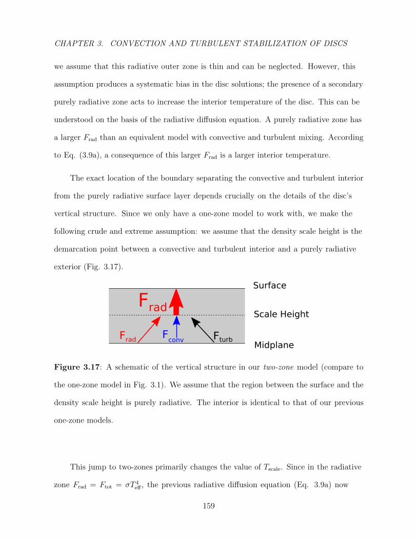
CHAPTER 3. CONVECTION AND TURBULENT STABILIZATION OF DISCS
we assume that this radiative outer zone is thin and can be neglected. However, this
assumption produces a systematic bias in the disc solutions; the presence of a secondary
purely radiative zone acts to increase the interior temperature of the disc. This can be
understood on the basis of the radiative diffusion equation. A purely radiative zone has
a larger Frad than an equivalent model with convective and turbulent mixing. According
to Eq. (3.9a), a consequence of this larger Frad is a larger interior temperature.
The exact location of the boundary separating the convective and turbulent interior
from the purely radiative surface layer depends crucially on the details of the disc’s
vertical structure. Since we only have a one-zone model to work with, we make the
following crude and extreme assumption: we assume that the density scale height is the
demarcation point between a convective and turbulent interior and a purely radiative
exterior (Fig. 3.17).
Figure 3.17: A schematic of the vertical structure in our two-zone model (compare to
the one-zone model in Fig. 3.1). We assume that the region between the surface and the
density scale height is purely radiative. The interior is identical to that of our previous
one-zone models.
This jump to two-zones primarily changes the value of Tscale. Since in the radiative
zone Frad = Ftot = σT 4eff , the previous radiative diffusion equation (Eq. 3.9a) now
159
CHAPTER 3. CONVECTION AND TURBULENT STABILIZATION OF DISCS
becomes
T (τ) = Teff ·[
3
4
(2
3+ τ
)]1/4
. (3.19)
For simplicity, we do not modify the other disc equations so the system can be solved
in the same way our one-zone models. Fig. 3.18 compares the one-zone and two-zone
disc solutions. As expected, the inclusion of a radiative outer zone pushes the convective
and turbulent solutions towards that of a purely radiative standard disc (i.e. the
two-zone solution lies in between the purely radiative disc and the homogeneously mixed
one-zone disc). The radiative outer zone ultimately pushes down the critical M of the
two-zone model towards lower values. However, our main result is unaffected; even in
two-zone discs, turbulently mixed discs are still significantly more stable than their
purely convective counterparts (compare critical M of left and right panels in 3.18).
160
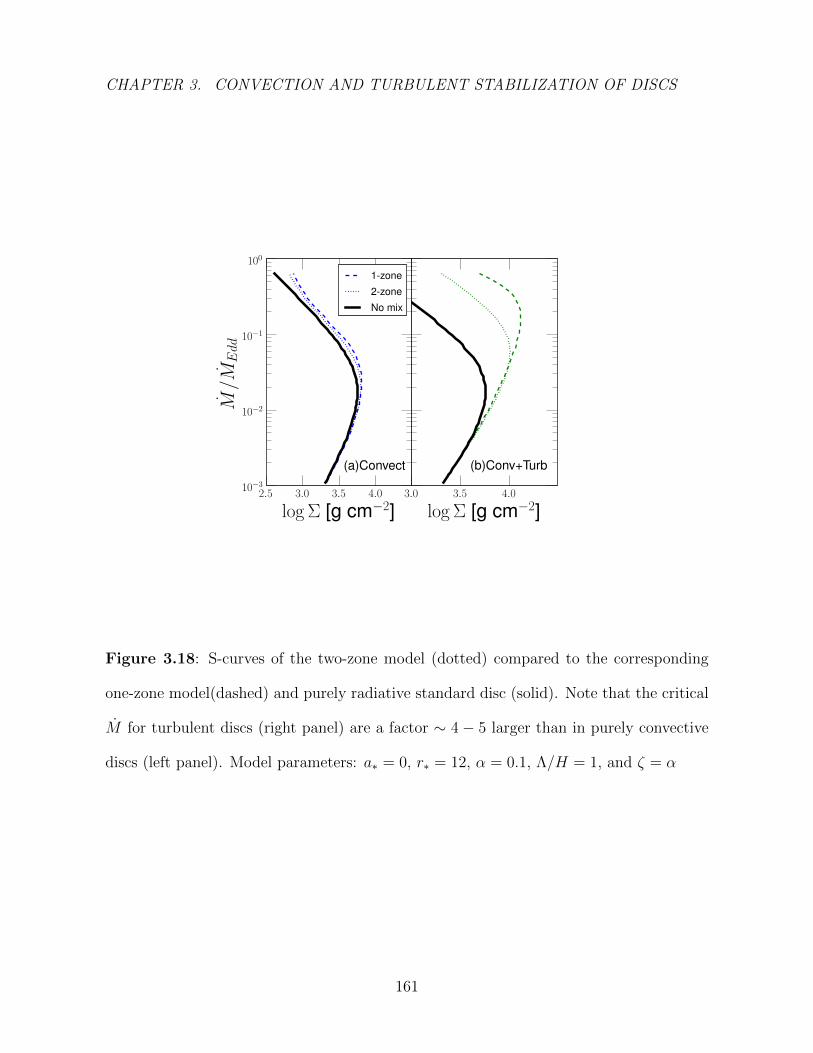
CHAPTER 3. CONVECTION AND TURBULENT STABILIZATION OF DISCS
Figure 3.18: S-curves of the two-zone model (dotted) compared to the corresponding
one-zone model(dashed) and purely radiative standard disc (solid). Note that the critical
M for turbulent discs (right panel) are a factor ∼ 4− 5 larger than in purely convective
discs (left panel). Model parameters: a∗ = 0, r∗ = 12, α = 0.1, Λ/H = 1, and ζ = α
161
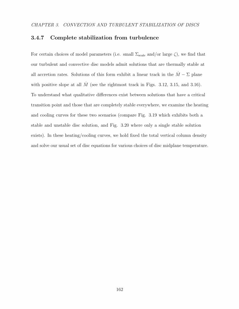
CHAPTER 3. CONVECTION AND TURBULENT STABILIZATION OF DISCS
3.4.7 Complete stabilization from turbulence
For certain choices of model parameters (i.e. small Σscale and/or large ζ), we find that
our turbulent and convective disc models admit solutions that are thermally stable at
all accretion rates. Solutions of this form exhibit a linear track in the M − Σ plane
with positive slope at all M (see the rightmost track in Figs. 3.12, 3.15, and 3.16).
To understand what qualitative differences exist between solutions that have a critical
transition point and those that are completely stable everywhere, we examine the heating
and cooling curves for these two scenarios (compare Fig. 3.19 which exhibits both a
stable and unstable disc solution, and Fig. 3.20 where only a single stable solution
exists). In these heating/cooling curves, we hold fixed the total vertical column density
and solve our usual set of disc equations for various choices of disc midplane temperature.
162
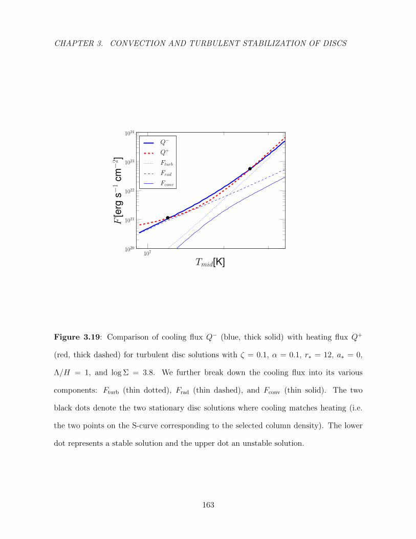
CHAPTER 3. CONVECTION AND TURBULENT STABILIZATION OF DISCS
Figure 3.19: Comparison of cooling flux Q− (blue, thick solid) with heating flux Q+
(red, thick dashed) for turbulent disc solutions with ζ = 0.1, α = 0.1, r∗ = 12, a∗ = 0,
Λ/H = 1, and log Σ = 3.8. We further break down the cooling flux into its various
components: Fturb (thin dotted), Frad (thin dashed), and Fconv (thin solid). The two
black dots denote the two stationary disc solutions where cooling matches heating (i.e.
the two points on the S-curve corresponding to the selected column density). The lower
dot represents a stable solution and the upper dot an unstable solution.
163

CHAPTER 3. CONVECTION AND TURBULENT STABILIZATION OF DISCS
Figure 3.20: Same as Fig. 3.19, but for a model with stronger turbulent mixing (ζ =
0.15). Here, the disc solution is completely thermally stable, so there is only one stationary
disc solution (black dot, which is thermally stable). The stability is due to the strong
turbulent cooling flux which ensures that Q− > Q+ at large Tmid.
We find for our turbulence model that the cooling scales as Fturb ∼ T 8 – comparable
to the scaling for heating in the radiation dominated regime Q+ ∼ T 8. If the action
of turbulence becomes sufficiently strong (represented in our model by taking a large
164
CHAPTER 3. CONVECTION AND TURBULENT STABILIZATION OF DISCS
value for ζ), then at high temperatures cooling always overtakes heating (see Fig. 3.20).
In these strongly turbulent cases, any positive temperature perturbations above the
equilibrium solution eventually cool back down to equilibrium. This eliminates the upper
unstable branch of solutions, leading to complete stability.
3.5 Summary
In this work, we have developed a simple one-zone model for black hole accretion discs
with both convective and turbulent vertical energy transport. We find that the action
of mixing from convection and turbulence provides a stabilizing effect on the disc,
pushing the threshold for thermal instability up towards higher accretion rates (compare
the critical M for different classes of discs in Fig. 3.4). For stellar mass black holes,
convection by itself provides only a modest boost to the thermal instability threshold,
only pushing the critical M to 5 per cent Eddington in the most favourable cases. On
the other hand, models that include additional mixing through MRI-induced turbulence
are much more stable. In some cases, we find that turbulent mixing pushes the threshold
for instability far above 10 per cent Eddington – even inducing complete stability in
the most extreme cases. A similarly strong effect is seen for supermassive black holes.
However, since the critical M for stability is lower by a factor of ∼ 10, even with the
effect of convection and turbulence, stable solutions are found only up to a few per cent
of Eddington.
Previous studies have shown that convective mixing in discs tends to provide a
stabilizing effect (Cannizzo 1992; Milsom, Chen & Taam 1994), which raises the critical
165
CHAPTER 3. CONVECTION AND TURBULENT STABILIZATION OF DISCS
accretion rate marking the onset of thermal instability. Since MRI-induced turbulence
is much more vigorous than convective turbulence, it is not surprising that turbulently
mixed discs experience a much stronger version of this stabilizing effect. Thus, we believe
that thermal stabilization from turbulent mixing is a promising mechanism for explaining
the apparent lack of instability in luminous (up to 50% of Eddington) black hole X-ray
binaries (Gierlinski & Done 2004). However, due to the mass scaling for the critical
accretion rate, we do not expect supermassive black holes to be stable at such high ac-
cretion rates - in our models they become unstable at around a few per cent of Eddington.
Finally, we stress that the precise value for the critical M found in our models
should not be taken too seriously. We are working in the framework of a one-zone
model (a rather severe approximation), and thus the quantitative details of our model
are quite sensitive to the choice of model parameters. Our main result is a qualitative
one – MRI-induced turbulent discs are much more stable than equivalent convective discs.
3.6 Acknowledgments
The authors would like to thank Robert Penna, Aleksander Sadowski, and Dmitrios
Psaltis for insightful discussions about disc convection. We thank the anonymous referee
for providing illuminating comments and helping us craft a much clearer paper. YZ
also thanks Tanmoy Laskar for helpful suggestions for improving the presentation of the
manuscript. YZ was supported by the Smithsonian Institution Endowment Funds. This
work was supported in part by NASA grant NNX11AE16G.
166
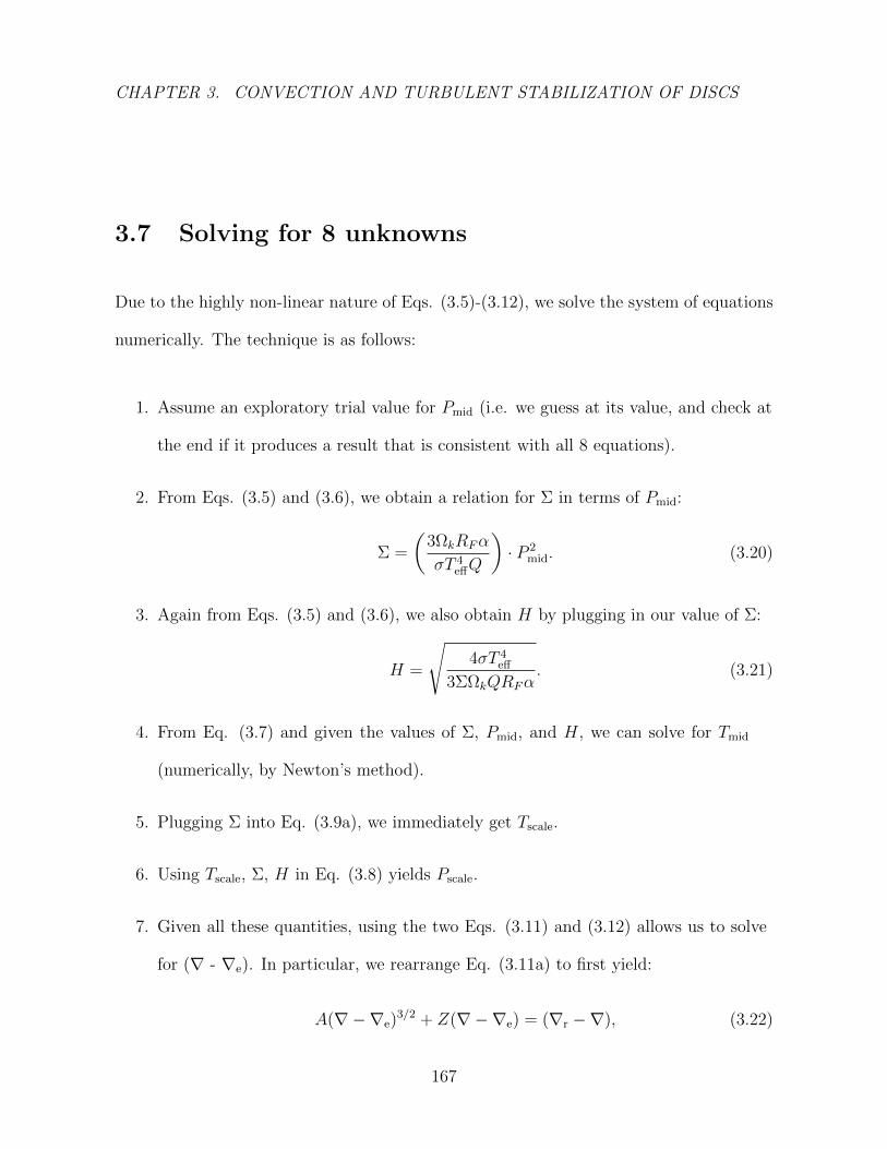
CHAPTER 3. CONVECTION AND TURBULENT STABILIZATION OF DISCS
3.7 Solving for 8 unknowns
Due to the highly non-linear nature of Eqs. (3.5)-(3.12), we solve the system of equations
numerically. The technique is as follows:
1. Assume an exploratory trial value for Pmid (i.e. we guess at its value, and check at
the end if it produces a result that is consistent with all 8 equations).
2. From Eqs. (3.5) and (3.6), we obtain a relation for Σ in terms of Pmid:
Σ =
(3ΩkRFα
σT 4effQ
)· P 2
mid. (3.20)
3. Again from Eqs. (3.5) and (3.6), we also obtain H by plugging in our value of Σ:
H =
√4σT 4
eff
3ΣΩkQRFα. (3.21)
4. From Eq. (3.7) and given the values of Σ, Pmid, and H, we can solve for Tmid
(numerically, by Newton’s method).
5. Plugging Σ into Eq. (3.9a), we immediately get Tscale.
6. Using Tscale, Σ, H in Eq. (3.8) yields Pscale.
7. Given all these quantities, using the two Eqs. (3.11) and (3.12) allows us to solve
for (∇ - ∇e). In particular, we rearrange Eq. (3.11a) to first yield:
A(∇−∇e)3/2 + Z(∇−∇e) = (∇r −∇), (3.22)
167
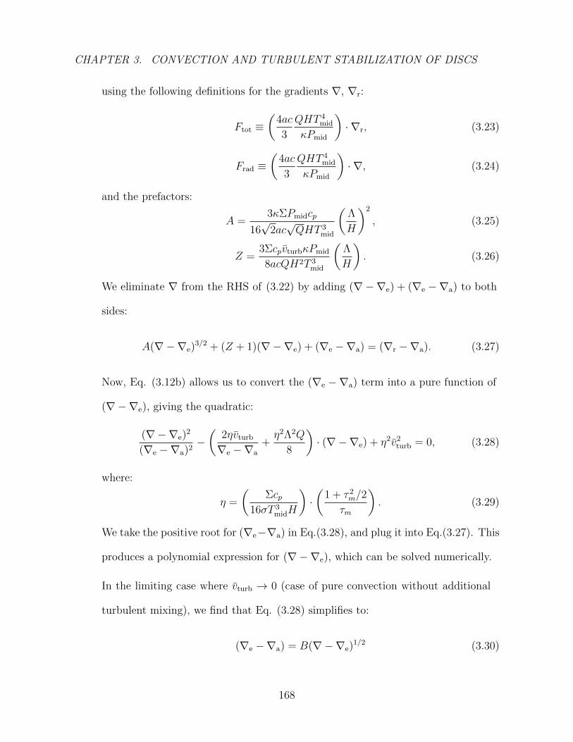
CHAPTER 3. CONVECTION AND TURBULENT STABILIZATION OF DISCS
using the following definitions for the gradients ∇, ∇r:
Ftot ≡(
4ac
3
QHT 4mid
κPmid
)· ∇r, (3.23)
Frad ≡(
4ac
3
QHT 4mid
κPmid
)· ∇, (3.24)
and the prefactors:
A =3κΣPmidcp
16√
2ac√QHT 3
mid
(Λ
H
)2
, (3.25)
Z =3ΣcpvturbκPmid
8acQH2T 3mid
(Λ
H
). (3.26)
We eliminate ∇ from the RHS of (3.22) by adding (∇−∇e) + (∇e −∇a) to both
sides:
A(∇−∇e)3/2 + (Z + 1)(∇−∇e) + (∇e −∇a) = (∇r −∇a). (3.27)
Now, Eq. (3.12b) allows us to convert the (∇e −∇a) term into a pure function of
(∇−∇e), giving the quadratic:
(∇−∇e)2
(∇e −∇a)2−(
2ηvturb
∇e −∇a
+η2Λ2Q
8
)· (∇−∇e) + η2v2
turb = 0, (3.28)
where:
η =
(Σcp
16σT 3midH
)·(
1 + τ 2m/2
τm
). (3.29)
We take the positive root for (∇e−∇a) in Eq.(3.28), and plug it into Eq.(3.27). This
produces a polynomial expression for (∇−∇e), which can be solved numerically.
In the limiting case where vturb → 0 (case of pure convection without additional
turbulent mixing), we find that Eq. (3.28) simplifies to:
(∇e −∇a) = B(∇−∇e)1/2 (3.30)
168
CHAPTER 3. CONVECTION AND TURBULENT STABILIZATION OF DISCS
where
B =
(32√
2σT 3mid
Σcp√Q
)(Λ
H
)−1(τm
1 + τ 2m/2
). (3.31)
Furthermore, vturb → 0 also implies Z → 0 and Eq.(3.27) becomes the following
cubic, which can be easily solved for (∇−∇e):
A(∇−∇e)3/2 + (∇−∇e) +B(∇−∇e)
1/2 = (∇r −∇a). (3.32)
8. Plugging (∇ − ∇e) back into Eq. (3.12) allows us to solve for both ∇ and ∇e
individually.
Now, armed with values for all 8 unknowns, we check to see if we made the correct
guess for Pmid by checking for consistency in ∇. A correct guess for Pmid will cause ∇
computed from the two probe points in Eq. (3.10) to be consistent with ∇ computed
from step (viii). Empirically, we find that this relation for ∇ is monotonic with Pmid,
and hence we are able to solve for the correct value of Pmid via bisection.
169
Chapter 4
HERO - A 3D General Relativistic
Radiative Postprocessor for
Accretion Discs around Black Holes
This thesis chapter originally appeared in the literature as
Y. Zhu, R. Narayan, A. Sadowski, D. Psaltis, submitted to
MNRAS, on Jan 14 2015
Abstract
HERO (Hybrid Evaluator for Radiative Objects) is a 3D general relativistic radiative
transfer code which has been tailored to the problem of analyzing radiation from
simulations of relativistic accretion discs around black holes. HERO is designed to be
used as a postprocessor. Given some fixed fluid structure for the disc (i.e. density and
170

CHAPTER 4. A 3D GENERAL RELATIVISTIC RADIATIVE CODE
velocity as a function of position from a hydrodynamics or magnetohydrodynamics
simulation), the code obtains a self-consistent solution for the radiation field and for
the gas temperatures using the condition of radiative equilibrium. The novel aspect of
HERO is that it combines two techniques: 1) a short characteristics (SC) solver that
quickly converges to a self consistent disc temperature and radiation field, with 2) a long
characteristics (LC) solver that provides a more accurate solution for the radiation near
the photosphere and in the optically thin regions. By combining these two techniques, we
gain both the computational speed of SC and the high accuracy of LC. We present tests
of HERO on a range of 1D, 2D and 3D problems in flat space and show that the results
agree well with both analytical and benchmark solutions. We also test the ability of the
code to handle relativistic problems in curved space. Finally, we discuss the important
topic of ray-defects, a major limitation of the SC method, and describe our strategy for
minimizing the induced error.
4.1 Introduction
Radiative transport (RT) plays a crucial role in astrophysics. It governs our primary
source of information about the cosmos, viz., the luminosities and spectra of cosmic
sources1. In addition, radiation acts as a channel for energy transport, shaping the
dynamics and impacting the evolution of astrophysical systems on all scales: stellar
evolution, stellar and galactic winds, super-Eddington accretion, epoch of reionization,
etc.
1We do receive additional information from cosmic rays, neutrinos and, hopefully soon, gravitational
waves, but these pale next to the enormous volume of information we receive via electromagnetic radiation.
171
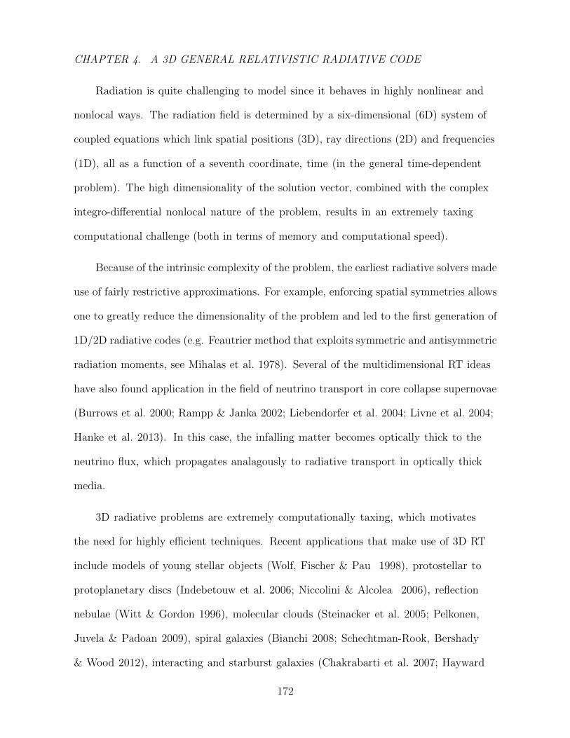
CHAPTER 4. A 3D GENERAL RELATIVISTIC RADIATIVE CODE
Radiation is quite challenging to model since it behaves in highly nonlinear and
nonlocal ways. The radiation field is determined by a six-dimensional (6D) system of
coupled equations which link spatial positions (3D), ray directions (2D) and frequencies
(1D), all as a function of a seventh coordinate, time (in the general time-dependent
problem). The high dimensionality of the solution vector, combined with the complex
integro-differential nonlocal nature of the problem, results in an extremely taxing
computational challenge (both in terms of memory and computational speed).
Because of the intrinsic complexity of the problem, the earliest radiative solvers made
use of fairly restrictive approximations. For example, enforcing spatial symmetries allows
one to greatly reduce the dimensionality of the problem and led to the first generation of
1D/2D radiative codes (e.g. Feautrier method that exploits symmetric and antisymmetric
radiation moments, see Mihalas et al. 1978). Several of the multidimensional RT ideas
have also found application in the field of neutrino transport in core collapse supernovae
(Burrows et al. 2000; Rampp & Janka 2002; Liebendorfer et al. 2004; Livne et al. 2004;
Hanke et al. 2013). In this case, the infalling matter becomes optically thick to the
neutrino flux, which propagates analagously to radiative transport in optically thick
media.
3D radiative problems are extremely computationally taxing, which motivates
the need for highly efficient techniques. Recent applications that make use of 3D RT
include models of young stellar objects (Wolf, Fischer & Pau 1998), protostellar to
protoplanetary discs (Indebetouw et al. 2006; Niccolini & Alcolea 2006), reflection
nebulae (Witt & Gordon 1996), molecular clouds (Steinacker et al. 2005; Pelkonen,
Juvela & Padoan 2009), spiral galaxies (Bianchi 2008; Schechtman-Rook, Bershady
& Wood 2012), interacting and starburst galaxies (Chakrabarti et al. 2007; Hayward
172
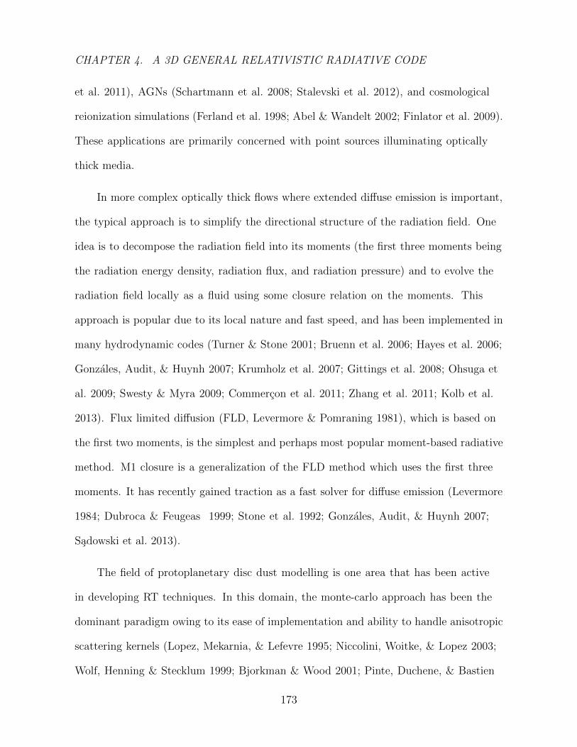
CHAPTER 4. A 3D GENERAL RELATIVISTIC RADIATIVE CODE
et al. 2011), AGNs (Schartmann et al. 2008; Stalevski et al. 2012), and cosmological
reionization simulations (Ferland et al. 1998; Abel & Wandelt 2002; Finlator et al. 2009).
These applications are primarily concerned with point sources illuminating optically
thick media.
In more complex optically thick flows where extended diffuse emission is important,
the typical approach is to simplify the directional structure of the radiation field. One
idea is to decompose the radiation field into its moments (the first three moments being
the radiation energy density, radiation flux, and radiation pressure) and to evolve the
radiation field locally as a fluid using some closure relation on the moments. This
approach is popular due to its local nature and fast speed, and has been implemented in
many hydrodynamic codes (Turner & Stone 2001; Bruenn et al. 2006; Hayes et al. 2006;
Gonzales, Audit, & Huynh 2007; Krumholz et al. 2007; Gittings et al. 2008; Ohsuga et
al. 2009; Swesty & Myra 2009; Commercon et al. 2011; Zhang et al. 2011; Kolb et al.
2013). Flux limited diffusion (FLD, Levermore & Pomraning 1981), which is based on
the first two moments, is the simplest and perhaps most popular moment-based radiative
method. M1 closure is a generalization of the FLD method which uses the first three
moments. It has recently gained traction as a fast solver for diffuse emission (Levermore
1984; Dubroca & Feugeas 1999; Stone et al. 1992; Gonzales, Audit, & Huynh 2007;
Sadowski et al. 2013).
The field of protoplanetary disc dust modelling is one area that has been active
in developing RT techniques. In this domain, the monte-carlo approach has been the
dominant paradigm owing to its ease of implementation and ability to handle anisotropic
scattering kernels (Lopez, Mekarnia, & Lefevre 1995; Niccolini, Woitke, & Lopez 2003;
Wolf, Henning & Stecklum 1999; Bjorkman & Wood 2001; Pinte, Duchene, & Bastien
173

CHAPTER 4. A 3D GENERAL RELATIVISTIC RADIATIVE CODE
2006). Monte-carlo RT has also been applied to the problem accretion discs, specifically
to handle the problem of modeling Compton scattering in disc coronas (Dolence et al.
2009; Schnittman & Krolik 2013; Ghosh 2013) as well as dust scattering of emission from
the Galactic centre (Odaka et al. 2011). The primary downside of this technique is the
computational expense and noise associated with photon statistics. The method is also
limited to modest optical depths.
The limitations of the various methods mentioned above led to the development of
more deterministic discretized finite-differencing methods (Stenholm, Stoerzer, & Wehrse
1991; Steinacker, Bacmann, & Henning 2002) and discrete ordinates characteristic
methods (Dullemond & Turolla 2000; Steinacker, Bacmann, & Henning 2002; Hayes &
Norman 2003; Vogler et al. 1982; Heinemann et al. 2006; Woitke, Kamp & Thi 2009;
Hayek et al. 2010; Davis et al. 2012; Jiang et al. 2014), which have a number of widely
discussed advantages. However, all of these methods suffer from the phenomenon of ”ray-
defects” (see appendix 4.6 for a detailed discussion). Another twist to the discretization
strategy involves expanding and evolving the radiation field as a combination of spherical
harmonics (Szu-cheng & Kuo-Nan 1982; Evans 1997; McClarren, Holloway, & Brunner
2008). Spherical harmonics respect rotational symmetry and therefore do not suffer from
the linear ray defect patterns that plague other discrete ordinate methods. The tradeoff
is that spherical methods typically suffer from artificial sidelobe patterns due to the
finite order cutoff used in taking the series expansion of the radiation field.
Raytracing methods are also used for predicting the observed flux from astrophysical
objects. These codes typically do not solve for the global radiation field within an
object; instead the focus is on calculating the apparent intensities that reach a distant
observer. In these codes, the typical assumption is to ignore scattering (i.e. to ignore
174
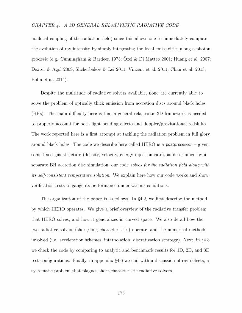
CHAPTER 4. A 3D GENERAL RELATIVISTIC RADIATIVE CODE
nonlocal coupling of the radiation field) since this allows one to immediately compute
the evolution of ray intensity by simply integrating the local emissivities along a photon
geodesic (e.g. Cunningham & Bardeen 1973; Ozel & Di Matteo 2001; Huang et al. 2007;
Dexter & Agol 2009; Shcherbakov & Lei 2011; Vincent et al. 2011; Chan et al. 2013;
Bohn et al. 2014).
Despite the multitude of radiative solvers available, none are currently able to
solve the problem of optically thick emission from accretion discs around black holes
(BHs). The main difficulty here is that a general relativistic 3D framework is needed
to properly account for both light bending effects and doppler/gravitational redshifts.
The work reported here is a first attempt at tackling the radiation problem in full glory
around black holes. The code we describe here called HERO is a postprocessor – given
some fixed gas structure (density, velocity, energy injection rate), as determined by a
separate BH accretion disc simulation, our code solves for the radiation field along with
its self-consistent temperature solution. We explain here how our code works and show
verification tests to gauge its performance under various conditions.
The organization of the paper is as follows. In §4.2, we first describe the method
by which HERO operates. We give a brief overview of the radiative transfer problem
that HERO solves, and how it generalizes in curved space. We also detail how the
two radiative solvers (short/long characteristics) operate, and the numerical methods
involved (i.e. acceleration schemes, interpolation, discretization strategy). Next, in §4.3
we check the code by comparing to analytic and benchmark results for 1D, 2D, and 3D
test configurations. Finally, in appendix §4.6 we end with a discussion of ray-defects, a
systematic problem that plagues short-characteristic radiative solvers.
175
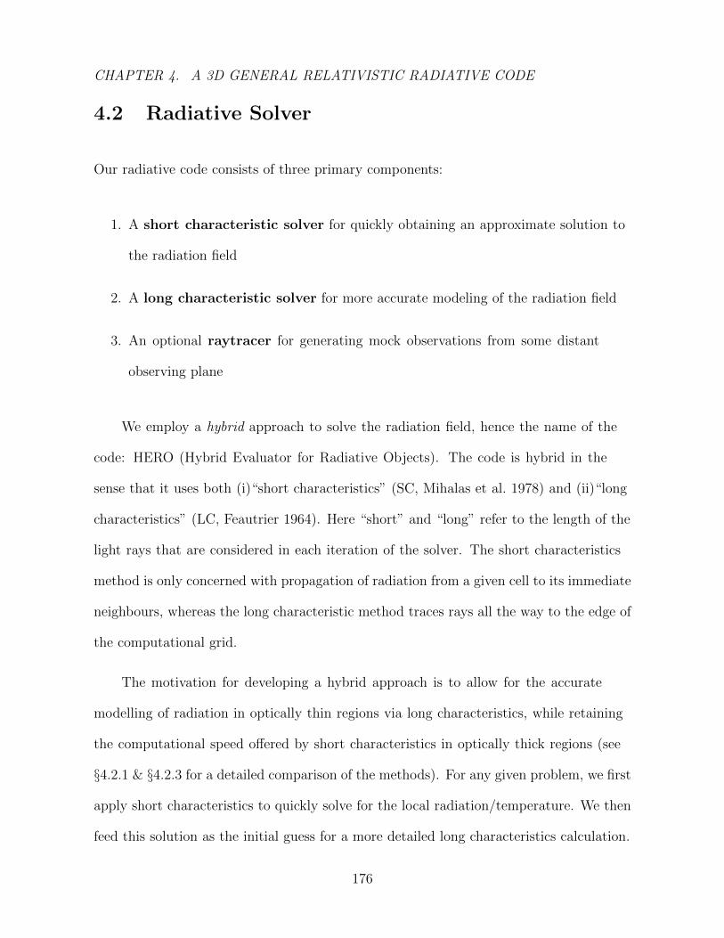
CHAPTER 4. A 3D GENERAL RELATIVISTIC RADIATIVE CODE
4.2 Radiative Solver
Our radiative code consists of three primary components:
1. A short characteristic solver for quickly obtaining an approximate solution to
the radiation field
2. A long characteristic solver for more accurate modeling of the radiation field
3. An optional raytracer for generating mock observations from some distant
observing plane
We employ a hybrid approach to solve the radiation field, hence the name of the
code: HERO (Hybrid Evaluator for Radiative Objects). The code is hybrid in the
sense that it uses both (i)“short characteristics” (SC, Mihalas et al. 1978) and (ii)“long
characteristics” (LC, Feautrier 1964). Here “short” and “long” refer to the length of the
light rays that are considered in each iteration of the solver. The short characteristics
method is only concerned with propagation of radiation from a given cell to its immediate
neighbours, whereas the long characteristic method traces rays all the way to the edge of
the computational grid.
The motivation for developing a hybrid approach is to allow for the accurate
modelling of radiation in optically thin regions via long characteristics, while retaining
the computational speed offered by short characteristics in optically thick regions (see
§4.2.1 & §4.2.3 for a detailed comparison of the methods). For any given problem, we first
apply short characteristics to quickly solve for the local radiation/temperature. We then
feed this solution as the initial guess for a more detailed long characteristics calculation.
176

CHAPTER 4. A 3D GENERAL RELATIVISTIC RADIATIVE CODE
Using such a hybrid approach allows us to combine the “best of both worlds.”
In addition to solving for the radiation field, in both SC and LC, we also solve for
a self-consistent gas temperature. The general idea is to loop back and forth between
solving for the radiation field given a fixed temperature structure, and solving for the
equilibrium temperature distribution given a fixed radiation field. This procedure is
iterated until convergence, leaving us with a self-consistent solution for both the radiation
and the temperature.
Our goal in developing HERO is to model/investigate the observed properties of
relativistic accretion discs around black holes, and to compare the radiative properties
of simulated discs with data collected by earthbound telescopes. Therefore, after
completing the SC and LC steps described above, the final step is to input the radiative
and temperature structure as computed from LC and to generate synthetic observations
of the disc as seen by a distant observer. For this stage we use the standard raytracing
approach (see §4.2.5 for details).
Due to the high temperatures present in accretion discs, Comptonization plays a
crucial role in determining the observed radiation from relativistic disc photospheres.
Because of the complex nature of the Compton scattering kernel, we defer discussion
of Comptonization to a follow-up paper, which will focus exclusively on explaining and
testing our relativistic scattering module.
177
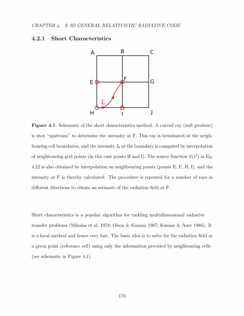
CHAPTER 4. A 3D GENERAL RELATIVISTIC RADIATIVE CODE
4.2.1 Short Characteristics
Figure 4.1: Schematic of the short characteristics method. A curved ray (null geodesic)
is shot “upstream” to determine the intensity at F. This ray is terminated at the neigh-
bouring cell boundaries, and the intensity I0 at the boundary is computed by interpolation
of neighbouring grid points (in this case points H and I). The source function S(τ ′) in Eq.
4.22 is also obtained by interpolation on neighbouring points (points E, F, H, I), and the
intensity at F is thereby calculated. The procedure is repeated for a number of rays in
different directions to obtain an estimate of the radiation field at F.
Short characteristics is a popular algorithm for tackling multidimensional radiative
transfer problems (Mihalas et al. 1978; Olson & Kunasz 1987; Kunasz & Auer 1988). It
is a local method and hence very fast. The basic idea is to solve for the radiation field at
a given point (reference cell) using only the information provided by neighbouring cells
(see schematic in Figure 4.1).
178
CHAPTER 4. A 3D GENERAL RELATIVISTIC RADIATIVE CODE
Ordinary Radiative Transfer Equation
To set the stage, we first discuss the standard case of flat space, where the radiative
transfer equation takes the form:
dIνds
= −(κν + σν)Iν + jν + σν
∫φν(Ω,Ω
′)Iν(Ω′)dΩ′. (4.1)
Here Iν is the intensity of a ray travelling along path s directed towards Ω; κν and σν are
the absorption and scattering coefficients; φν is the scattering shape function, normalized
such that∫φν(Ω,Ω
′)dΩ′ = 1; and jν is the emission coefficient. Typically, Eq.4.1 is
simplified to the form
dIνdτν
= −Iν + Sν , (4.2)
where the the optical depth τν is given by
dτν = (κν + σν)ds, (4.3)
and the source function Sν is defined as
Sν =jν + σν
∫φν(Ω,Ω
′)Iν(Ω′)dΩ′
κν + σν. (4.4)
In the case of isotropic scattering, φν = 1/4π, and the scattering term simplifies to∫φν(Ω,Ω
′)Iν(Ω′)dΩ′ =
1
4π
∫Iν(Ω
′)dΩ′ ≡ Jν , (4.5)
where Jν is the angle-averaged mean intensity. We assume isotropic scattering in all of
the work reported here. We further assume a thermal source, for which the emissivity is
given by jν = κνBν(T ), where Bν(T ) is the Planck function corresponding to the local
temperature T of the medium. With these two simplifications, the source function can
be compactly rewritten as:
Sν = ενBν + (1− εν)Jν , (4.6)
179

CHAPTER 4. A 3D GENERAL RELATIVISTIC RADIATIVE CODE
where εν is the photon interaction destruction probability, given by the ratio of the
absorption and total opacity:
εν ≡κν
κν + σν. (4.7)
To avoid confusion with summation indices, in the remainder of this paper we will no
longer use a subscript ν to note the frequency dependence of radiative quantities. Unless
otherwise stated, this will apply to all subsequent intensities, opacities, source functions,
and emissivities.
Covariant Formulation of the Radiative Transfer Equation
Because HERO has been developed for relativistic problems, we use a generalization of
the radiative transfer equation that accounts for relativistic effects such as light bending
and doppler boosting. The generalization of the radiative transfer equation to curved
space has been discussed in the literature (Mihalas & Mihalas 1984; Lindquist 1966), but
we give a brief primer here for completeness. Starting from the time dependent version
of Eq. 4.1:
1
c
dI
dt+ (n · ∇)I = G, (4.8)
where G on the righthand side contains all scattering and absorption source terms that
interact with the radiation field, and n is a normalized 3-vector denoting the propagation
direction of photons. We can rewrite Eq. 4.8 in a more revealing form by introducing
the direction 4-vector kα whose orthonormal form is (note that k · k = 0):
kα = (1, n). (4.9)
This lets us rewrite the RT equation (setting c = 1) as:
kαd
dxαI = G ≡ −(κ+ σ)I + j + σJ. (4.10)
180

CHAPTER 4. A 3D GENERAL RELATIVISTIC RADIATIVE CODE
By considering the Lorentz transformation properties of the various quantities,
Eq.4.10 can be recast in an invariant form (see Mihalas & Mihalas 1984, §7.1):
pα∂
∂xαI = G, (4.11)
where the photon 4-momentum pα = hνkα takes on the role of the propagation 4-vector.
Instead of the usual definitions of intensity I and source term G, this equation considers
their corresponding relativistically invariant versions,
I = I/ν3, G = hG/ν2, (4.12)
where the scaling of I is determined by photon number conservation in phase space. The
(hν)−2 scaling for G arises after transforming Eq.4.10 to use I and allows us to construct
the invariant scalings for the absorption and scattering coefficients as:
kν = hνκν , sν = hνσν , (4.13)
and for the emissivity and source function,
jν = hjν/ν2, S = S/ν3. (4.14)
In terms of these new quantities, the invariant source G becomes
G = −(k + s)(I − S). (4.15)
For convenience, since we usually work with comoving quantities, κc, σc, Sc, we can
instead write G as:
G = −hνc(κc + σc)
[−I +
Sc
ν3c
]= pαuα(κc + σc)
[−I +
Sc
ν3c
], (4.16)
181
CHAPTER 4. A 3D GENERAL RELATIVISTIC RADIATIVE CODE
where uµ is the four-velocity of the fluid. Eq. 4.11 is in manifestly covariant form and
the generalization to curved space is simply accounted for by replacing the directional
derivative ∂/∂xα with the covariant derivative:
D
Dxα=
∂
∂xα− Γγαβp
β ∂
∂pγ, (4.17)
evaluated along a null geodesic (Lindquist 1966). The general covariant form of the RT
equation then takes the form:
pαD
DxαI = G (4.18)
We can further simplify the above expression by using the photon geodesic equation,
dpγ
dλ= −Γγαβp
αpβ, (4.19)
where λ is an affine parameter defined by pα = dxα/dλ. Using Eq. 4.19 to eliminate the
Christoffel symbols in Eq. 4.17, the RT equation becomes:
pα∂I∂xα
+dpα
dλ
∂I∂pα
= G. (4.20)
Finally, using the chain rule for partial differentiation, we obtain the very simple equation
dIdλ
= G. (4.21)
This is the form of the covariant RT equation that we employ in HERO. The only
point that requires some care is choosing the correct frequency when evaluating the
source term G. For instance, if we wish to evaluate I at frequency ν in the lab frame,
but we compute G in the fluid comoving frame (the natural frame since the opacity is
defined there), then νc in Eq. 4.16 must be chosen such that it corresponds to the lab
frame ν used to label I.
182
CHAPTER 4. A 3D GENERAL RELATIVISTIC RADIATIVE CODE
4.2.2 Implementation of Short Characteristics
Given a ray in the reference cell F, we compute the upstream location where it intersects
the boundary of that cell (see Fig. 4.1) and use this location to determine the relative
weights contributed by each of the four nearest neighbours on that boundary. In flat
space, it is possible to write down an analytical formula for the intersection point (e.g.
Dullemond & Turolla 2000), but there is no generalization in terms of simple functions
for curved space. HERO does the calculation numerically.
Although this is computationally somewhat expensive, it needs to be done only once
as part of the initialization steps. The information from this initial computation is saved
and used repeatedly during the SC iterations. Given the intersection of a ray with the
nearest neighbour cell boundary, we compute the intensity of this ray in the reference
cell F using the radiative transfer equation (Eq. 4.21):
IF = I0 exp(−τ0) +
∫ τ0
0
S(τ ′) exp(−τ ′)dτ ′, (4.22)
where I0 is the incoming intensity at the boundary, and τ0 is the total optical depth of
the photon path leading from the boundary to point F (computed using the average of
the central and boundary opacities). The intensity I0 is computed by interpolating from
the four boundary points. Our current implementation of short characteristics uses linear
interpolations at various stages (this is easily improved in the future). In this spirit, the
integral evaluation in Eq. 4.22 is computed as∫ τ
0
S(τ ′) exp(−τ ′)dτ ′
=e−τ (S0 − Sτ (1 + τ)) + S0(τ − 1) + Sτ
τ, (4.23)
which is the analytic solution when the source function S varies linearly with τ along the
183
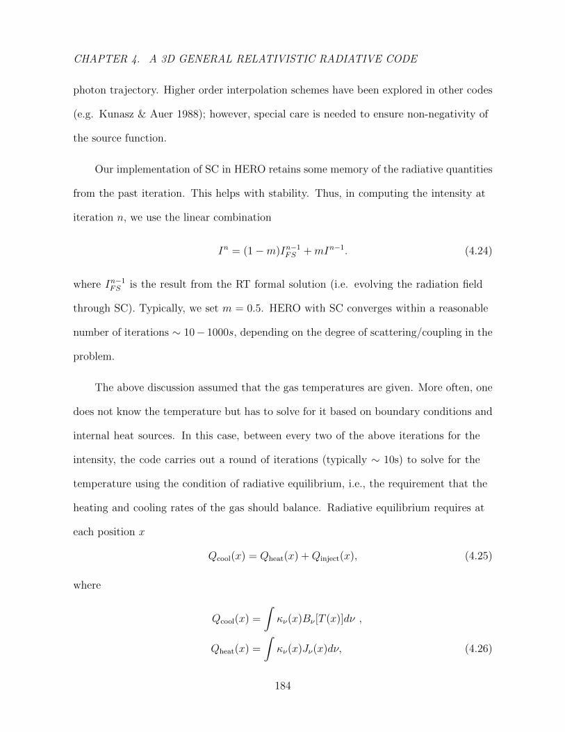
CHAPTER 4. A 3D GENERAL RELATIVISTIC RADIATIVE CODE
photon trajectory. Higher order interpolation schemes have been explored in other codes
(e.g. Kunasz & Auer 1988); however, special care is needed to ensure non-negativity of
the source function.
Our implementation of SC in HERO retains some memory of the radiative quantities
from the past iteration. This helps with stability. Thus, in computing the intensity at
iteration n, we use the linear combination
In = (1−m)In−1FS +mIn−1. (4.24)
where In−1FS is the result from the RT formal solution (i.e. evolving the radiation field
through SC). Typically, we set m = 0.5. HERO with SC converges within a reasonable
number of iterations ∼ 10− 1000s, depending on the degree of scattering/coupling in the
problem.
The above discussion assumed that the gas temperatures are given. More often, one
does not know the temperature but has to solve for it based on boundary conditions and
internal heat sources. In this case, between every two of the above iterations for the
intensity, the code carries out a round of iterations (typically ∼ 10s) to solve for the
temperature using the condition of radiative equilibrium, i.e., the requirement that the
heating and cooling rates of the gas should balance. Radiative equilibrium requires at
each position x
Qcool(x) = Qheat(x) +Qinject(x), (4.25)
where
Qcool(x) =
∫κν(x)Bν [T (x)]dν ,
Qheat(x) =
∫κν(x)Jν(x)dν, (4.26)
184
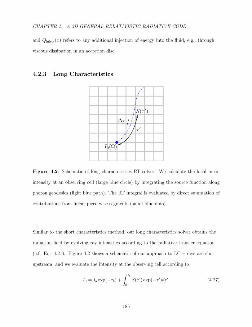
CHAPTER 4. A 3D GENERAL RELATIVISTIC RADIATIVE CODE
and Qinject(x) refers to any additional injection of energy into the fluid, e.g., through
viscous dissipation in an accretion disc.
4.2.3 Long Characteristics
Figure 4.2: Schematic of long characteristics RT solver. We calculate the local mean
intensity at an observing cell (large blue circle) by integrating the source function along
photon geodesics (light blue path). The RT integral is evaluated by direct summation of
contributions from linear piece-wise segments (small blue dots).
Similar to the short characteristics method, our long characteristics solver obtains the
radiation field by evolving ray intensities according to the radiative transfer equation
(c.f. Eq. 4.21). Figure 4.2 shows a schematic of our approach to LC – rays are shot
upstream, and we evaluate the intensity at the observing cell according to
I0 = Ib exp(−τb) +
∫ τb
0
S(τ ′) exp(−τ ′)dτ ′. (4.27)
185
CHAPTER 4. A 3D GENERAL RELATIVISTIC RADIATIVE CODE
The above expression is identical to our SC calculation (Eq.4.22), except that Ib now
represents the intensity distribution at the grid boundaries and the ray integral continues
past the immediate neighbouring cells to traverse the entire spatial domain. The integral
in Eq. 4.27 is evaluated in discrete steps (τ ′ → τ ′ + ∆τ), where each source-function
piece is evaluated using the same linear interpolation scheme as used in SC (Eq. 4.23).
One major difference between our LC and SC solvers is the choice of angular grid.
In SC we used a fixed angular resolution (NA = 80, see §4.2.7) for all cells. This fairly
low resolution choice is adequate (though only barely) in SC since one only needs to
resolve the neighbouring 27 grid cells. In LC, since the rays traverse the entire spatial
domain, much higher angular resolution is needed to resolve the emission from distant
source cells. This becomes particularly problematic with spherical coordinates where
the grid spans a few decades in radius. Cells located at larger radii have a difficult time
“seeing” the inner regions unless one takes care in choosing the ray directions.
Our solution is to dynamically set the angular resolution used by the LC solver such
that there is sufficient coverage to resolve all the cells within the domain. Consider, as a
typical example, a 3D grid in spherical coordinates which extends from an inner radius
rin to an outer radius rout rin. The radial dynamic range may be up to three decades,
as in some of the examples described later. Let us suppose that our spherical spatial grid
uses uniform angular spacing in θ, with Nθ cells, and logarithmic spacing in radius with
Nr . Nθ cells per decade. Consider a cell at some radius r. For this cell, the apparent
density of other cells as viewed in its local ”sky” is highly anisotropic. For rays traveling
from the direction of the coordinate centre, this cell needs to sample the local radiation
field with an angular resolution of order ∆θres ∼ rin/rNθ in order to adequately sample
the contribution of all the cells at the centre. In the opposite direction, however, an
186
CHAPTER 4. A 3D GENERAL RELATIVISTIC RADIATIVE CODE
angular resolution of order ∼ 1/Nθ is sufficient.
The above requirement can be achieved by designing a suitable angular tiling of
the sky. One simple prescription is to vary the angular resolution ∆θres as a function of
direction χ relative to the local radius vector as follows:
∆θres =f
Nθ
(rin
r+ χ
), (4.28)
where f controls the factor by which we oversample to reduce noise. Usually f = 1 is
adequate, however even with this relatively low resolution, the number of tiles varies
from ∼ N2θ for the innermost radial grid cells to several orders of magnitude larger for
outer cells. The increase in resolution at the outer cells is needed in order to resolve the
interior. The average number of rays per cell is thus a factor of 100 or more larger than
the NA = 80 rays that we consider with short characteristics. In addition, each ray in
LC traverses the entire grid, compared to just one cell with SC. For both reasons, one
iteration of LC often takes 104 times more computation time than one iteration of SC!
On the other hand, one iteration of LC moves the solution much closer to convergence
since information is propagated across the entire grid.
The main weakness of LC is its inability to handle optically thick regions in
scattering-dominated problems. This is because of the huge number of iterations needed
to model properly the diffusion process. Since LC cannot be feasibly run for more
than a few dozen iterations, it cannot be used to update radiative information deep
inside optically thick objects. Luckily, it is precisely in this optically thick regime where
short characteristics is free from the ray-defect problem and can be trusted to produce
unbiased results. This motivates our hybrid scheme: first we run many iterations of
short characteristics to resolve the complete diffusive process and to correctly obtain the
187
CHAPTER 4. A 3D GENERAL RELATIVISTIC RADIATIVE CODE
radiation field in the optically thick parts of the problem; second we run a few passes of
LC to ensure that the optically thin regions of the radiation field are handled accurately
and are devoid of ray-defects.
4.2.4 Acceleration Schemes
The radiative quantities S and J are inextricably linked. For future reference, we
quantify the dependence of J on S by means of a Λ operator, defined such that
Ji = ΛjiSj, (4.29)
where the sub/superscripts denote grid cells. Each iteration of the radiative solver2 acts
as Λ, describing how J is related to S. However, since S itself has a scattering term, it
needs to be updated along with J . Writing this explicitly (c.f. Eq. 4.6),
Sn+1 = (1− ε)Jn + εB
= (1− ε)Λ[Sn] + εB. (4.30)
By switching between solving for J as a function of S (Eq. 4.29), and for S as a function
of J (Eq. 4.30), we seek to find a stationary self-consistent solution for all our radiative
quantities. Unfortunately, simply applying these two transformations one after the other
and iterating has well known convergence issues whenever scattering strongly dominates
(say with ε < 10−2).
To avoid slow convergence, acceleration schemes are often employed. Accelerated
lambda iteration (ALI) is one such technique. To understand the idea behind ALI,
2In both SC and LC, the mean intensity term J is evaluated by averaging I via Eq.4.5
188
CHAPTER 4. A 3D GENERAL RELATIVISTIC RADIATIVE CODE
rewrite Eq. 4.30 so as to isolate S:
S = [1− (1− ε)Λ]−1[εB]. (4.31)
Formally, one can obtain the complete solution by evaluating the inverse matrix on the
right hand side of Eq.4.31 and calculating S from B. Then evaluating Eq. 4.29 gives J .
However, in 3D, Λ is an enormous matrix and it is impractical to carry out full matrix
inversion. Instead, ALI considers an approximate lambda operator, typically chosen
to be the diagonal component Λii (i.e. the contribution to the local J from solely the
local S – usually the largest component). Denoting the shift in our old formal solution
without acceleration as ∆SFS = Sn+1i − Sni , solving the system taking into account Λ
yields (see Hubeny 2003 for details):
∆SALIi =∆SFS
1− (1− εi)Λii
. (4.32)
To obtain the diagonal of the Λ operator, we consider:
Λii =JiiSi, (4.33)
where Jii represents the local contribution to J from the source function within the
reference grid cell. This self-illumination contribution to J is the following sum over the
NA ray angles considered:
Jii =1
NA
NA∑i=1
I locali , (4.34)
where I is evaluated by summing up all local sources within the cell:
I locali =
∫ τ0
0
S(τ ′) exp(−τ ′)dτ ′. (4.35)
ALI is crucial for scattering-dominated problems whenever ε < 0.01 – see convergence
tests in §4.3.2. Even with ALI, we often need to run hundreds of iterations before the
189

CHAPTER 4. A 3D GENERAL RELATIVISTIC RADIATIVE CODE
solution settles down and converges. This is feasible with SC, which is quite fast, but
not practical with the much slower LC. The convergence criterion that we use is:
max
(|∆Si|Si
)≤ δc, (4.36)
where the convergence level δc is preset to a desired accuracy level (typically δc = 10−4).
4.2.5 Raytracing
At the end of the day, we wish to calculate images and compute synthetic spectra from
our radiating objects. This is accomplished by means of raytracing from some distant
observation plane. We consider a large number of rays arriving at the observer and trace
each backwards in time to determine its trajectory and point of origin. Then, using the
radiative transfer equation and the source function as calculated via the LC method, we
compute the observed intensity of each ray. Finally, we combine the rays to construct
the observed image of the disc as well as the spectrum of the source. These synthetic
results, which are easily calculated for different viewing angles, can be directly compared
to observations of accretion discs.
Photon trajectories are handled by numerically evaluating the null geodesic equation
Eq. 4.19 (a second order PDE in x and p):
d2xα
dλ2= −Γαβγp
βpγ
with pα =dxα
dλ. (4.37)
The emission seen at the observer plane is obtained by summing up the emissivity along
the ray paths (same exercise as Eq. 4.27). This yields a grid of ray intensities (”image”
190

CHAPTER 4. A 3D GENERAL RELATIVISTIC RADIATIVE CODE
of the system) as projected on the observation plane. Integrating all the rays generates
the final observed spectrum via
Fν =
∫IνcosθdΩ, (4.38)
where θ ≈ 0 is the normal incident angle of the ray at the observer plane, Iν is the
intensity at the observer plane, and dΩ is the angular size of a single pixel at the observer
plane.
4.2.6 Frequency Discretization
HERO is set up to handle frequency dependent opacities. Both the computational
cost and memory requirement scale linearly with nF the number of frequency bins.
All radiative quantities (opacities, intensities, source functions) are calculated for the
same discrete set of frequencies. The code could be set up to handle group mean
opacities and emissivities with their appropriate quadrature weights to handle more
complex line emission problems. In problems where there is frequency coupling (i.e.
gravitational/doppler shifting) the redistribution of photons is handled by linear
interpolation. Our typical choice for the frequency grid is a total range of 6 decades with
a resolution of 10 points per decade (60 frequency bins).
4.2.7 Angular Discretization
The angular setup of our code differs based on the dimensionality of the problem that is
being solved.
191
CHAPTER 4. A 3D GENERAL RELATIVISTIC RADIATIVE CODE
1D Angles
In 1D, we solve plane parallel slab problems which are actually 3D problems that can be
collapsed down to 1D by invoking translational and azimuthal symmetry. We subdivide
the 4π steradian sphere into equal solid angle slices in θ; thus, we set our angle spacing
dθ such that sin θdθ = 2/NA.
2D Angles
In all the 2D test problems described in this paper, the rays are considered to live in a
flat 2D space, so we do not consider the 3D solid angle at all. We choose our angle grid
so as to cover uniformly the full 2π of the 2D plane. We use simple linear interpolation
on 2D angles to handle the mixing of angles when rays travel from one cell to another.
3D Angles
The goal is to subdivide the 4π sphere of solid angle into NA solid angle wedges. A few
common approaches include bisecting octants, following a ”spiral” that winds around the
sphere from the two poles, or a special grid of latitudes/longitudes. All these methods
approximately achieve the required goal, but they suffer from undesirable patterns of
symmetry lines or ”seams” on the surface of the sphere. To sidestep this issue, we obtain
our angular grid via a numerical approach.
The strategy that we employ is to deposit NA fictitious charged particles constrained
to move on the surface of a sphere, with initial positions set by simple heuristics (equal
proper length spacings in θ, φ coordinates). Then, we allow the particles to evolve
192
CHAPTER 4. A 3D GENERAL RELATIVISTIC RADIATIVE CODE
over time under their mutual inter-particle electrostatic forces until they settle on an
equilibrium configuration. This naturally produces a set of positions that are nearly
equidistant from one another. We use these positions to specify the angular grid (see Fig
4.3 for an example with NA = 80).
For relativistic problems where light bending introduces mixing between different
angle bins, or for curvilinear coordinate grid setups that invoke angle grids fixed along
the locally rotated unit direction vectors, we handle angular interpolation via linear
combinations. For a ray with a given unit direction vector ψ, there will always by a set
of 3 angular points (ψ1, ψ2, ψ3) on the 4π sphere which defines a triangle enclosing ψ. We
find the angles (ψ1, ψ2, ψ3) by simply locating the 3 angles with the largest dot product
to ψ in the angle grid.
Once the three vertices of the triangle have been identified, we decompose ψ as a
linear combination of ψ1, ψ2, ψ3:
ψ = c1ψ1 + c2ψ2 + c3ψ3. (4.39)
The coefficients c1, c2, c3 (after renormalizing to satisfy c1 + c2 + c3 = 1) are then used
as the interpolation weights. In rare cases (i.e. when ψ is slightly outside the boundary
of the triangle formed by ψ1, ψ2, ψ3), the interpolation weights may be slightly negative.
For stability purposes, we clip any negative weights to zero.
In Fig. 4.3, we show how our linear interpolation scheme handles an example
intensity pattern. Notice that in the slowly-varying equatorial regions, the interpolated
result provides a much better match to the exact intensity distribution than simply using
a discretized version of the intensity field. The linear reconstruction does poorly when
the radiation field fluctuates on angular scales smaller than a single beamwidth of the
193
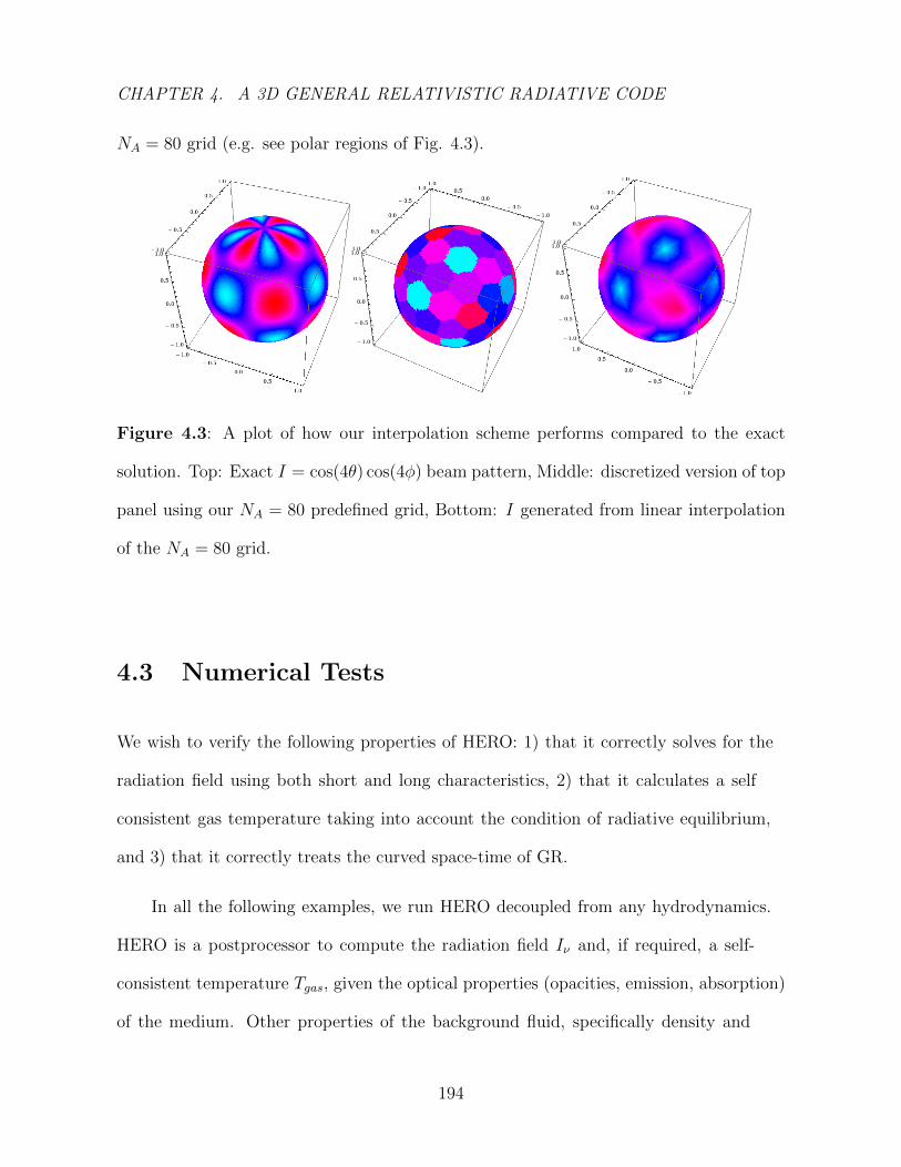
CHAPTER 4. A 3D GENERAL RELATIVISTIC RADIATIVE CODE
NA = 80 grid (e.g. see polar regions of Fig. 4.3).
Figure 4.3: A plot of how our interpolation scheme performs compared to the exact
solution. Top: Exact I = cos(4θ) cos(4φ) beam pattern, Middle: discretized version of top
panel using our NA = 80 predefined grid, Bottom: I generated from linear interpolation
of the NA = 80 grid.
4.3 Numerical Tests
We wish to verify the following properties of HERO: 1) that it correctly solves for the
radiation field using both short and long characteristics, 2) that it calculates a self
consistent gas temperature taking into account the condition of radiative equilibrium,
and 3) that it correctly treats the curved space-time of GR.
In all the following examples, we run HERO decoupled from any hydrodynamics.
HERO is a postprocessor to compute the radiation field Iν and, if required, a self-
consistent temperature Tgas, given the optical properties (opacities, emission, absorption)
of the medium. Other properties of the background fluid, specifically density and
194

CHAPTER 4. A 3D GENERAL RELATIVISTIC RADIATIVE CODE
velocity, are assumed to be given and fixed. It is also assumed that the system is
time-independent, so we effectively solve for the steady state solution for the radiation.
We are particularly interested in problems where scattering dominates the opacity
(as is often true with relativistic accretion flows), leading to diluted-blackbody radiation
fields. Due to the complicated nature of scattering, many iterations are needed for the
radiative solver to converge. This makes scattering problems ideally suited to test the
convergence properties of the code. We describe below a series of 1D, 2D and 3D tests.
4.3.1 1D Plane-parallel Grey Atmosphere
Scattering problems are in general very difficult to solve due to the integro-differential
nature of the scattering kernel in the radiative transfer equation (see righthand side of
Eq. 4.1). As such, there are very few examples that have closed form analytic solutions.
The 1D plane-parallel isothermal slab with grey opacity turns out to be one
particularly simple case with a well known closed form solution in the two-stream limit
(c.f. §1 Rybicki & Lightman 1979). There is also a semi analytic solution in the limit of
infinite angles. For this problem, all quantities, T, κ, σ, are uniform within the medium,
leading to a solution that is only a function of the optical depth: dτ = (κ+ σ)dz. Under
the two-stream approximation, and using the Eddington approximation to close the
radiative moment equations, the analytic solution for the mean intensity is given by
J(τ) = B
[1− exp(−
√3ετ)
1 +√ε
], (4.40)
where B is the thermal blackbody source function, τ is the total optical depth from the
surface, and ε is the photon interaction destruction probability given by Eq.4.7.
195

CHAPTER 4. A 3D GENERAL RELATIVISTIC RADIATIVE CODE
Note the exponential transition in τ that separates a thermal interior from a
dilute-blackbody surface layer. In Figure 4.4, we show solutions computed by HERO
compared to Eq. 4.40. The τ = 0 surface outer boundary condition was set to have
zero ingoing flux, and the innermost τ = 105 boundary was set to J = B for some
fixed B. The agreement between the numerical and analytical solutions is quite good
(∼ 1% errors) with a systematic trend of larger errors in low ε systems. These low ε
atmospheres are highly scattering dominated and the induced systematic error is simply
a consequence of the nonlocal nature of scattered radiation.
10-2 10-1 100 101 102 103 104 105
τ
10-4
10-3
10-2
10-1
100
J/B
ε=10−1
ε=10−3
ε=10−5
ε=10−7
Figure 4.4: J computed from HERO (dashed lines) compared with the analytic solu-
tion (solid lines) for a plane parallel scattering atmosphere described under the 2-stream
approximation. Four values of ε (see Eq. 4.7) are shown.
196
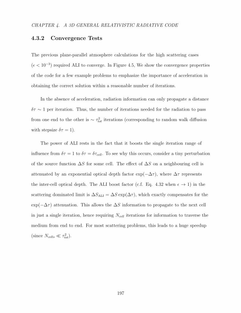
CHAPTER 4. A 3D GENERAL RELATIVISTIC RADIATIVE CODE
4.3.2 Convergence Tests
The previous plane-parallel atmosphere calculations for the high scattering cases
(ε < 10−3) required ALI to converge. In Figure 4.5, We show the convergence properties
of the code for a few example problems to emphasize the importance of acceleration in
obtaining the correct solution within a reasonable number of iterations.
In the absence of acceleration, radiation information can only propagate a distance
δτ ∼ 1 per iteration. Thus, the number of iterations needed for the radiation to pass
from one end to the other is ∼ τ 2tot iterations (corresponding to random walk diffusion
with stepsize δτ = 1).
The power of ALI rests in the fact that it boosts the single iteration range of
influence from δτ = 1 to δτ = δτcell. To see why this occurs, consider a tiny perturbation
of the source function ∆S for some cell. The effect of ∆S on a neighbouring cell is
attenuated by an exponential optical depth factor exp(−∆τ), where ∆τ represents
the inter-cell optical depth. The ALI boost factor (c.f. Eq. 4.32 when ε → 1) in the
scattering dominated limit is ∆SALI = ∆S exp(∆τ), which exactly compensates for the
exp(−∆τ) attenuation. This allows the ∆S information to propagate to the next cell
in just a single iteration, hence requiring Ncell iterations for information to traverse the
medium from end to end. For most scattering problems, this leads to a huge speedup
(since Ncells τ 2tot).
197
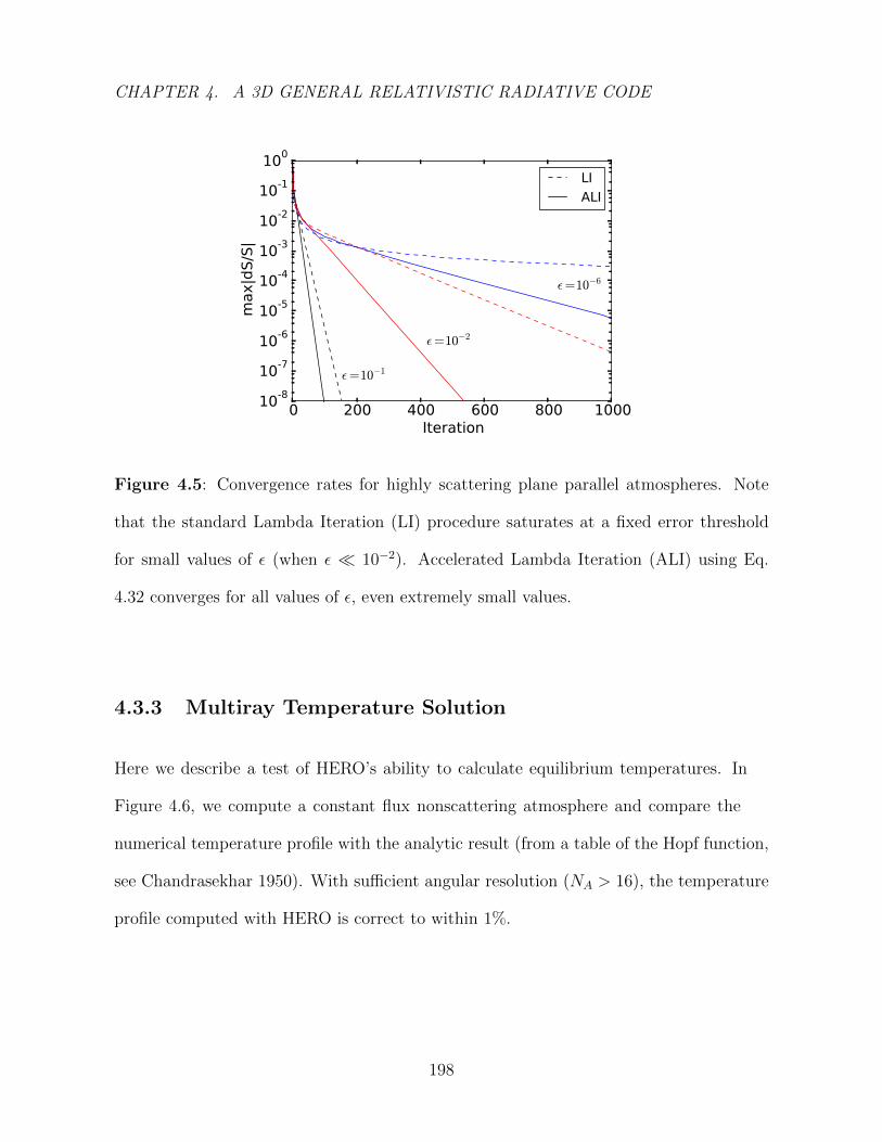
CHAPTER 4. A 3D GENERAL RELATIVISTIC RADIATIVE CODE
0 200 400 600 800 1000Iteration
10-8
10-7
10-6
10-5
10-4
10-3
10-2
10-1
100
max
|dS/
S|
ε=10−1
ε=10−2
ε=10−6
LIALI
Figure 4.5: Convergence rates for highly scattering plane parallel atmospheres. Note
that the standard Lambda Iteration (LI) procedure saturates at a fixed error threshold
for small values of ε (when ε 10−2). Accelerated Lambda Iteration (ALI) using Eq.
4.32 converges for all values of ε, even extremely small values.
4.3.3 Multiray Temperature Solution
Here we describe a test of HERO’s ability to calculate equilibrium temperatures. In
Figure 4.6, we compute a constant flux nonscattering atmosphere and compare the
numerical temperature profile with the analytic result (from a table of the Hopf function,
see Chandrasekhar 1950). With sufficient angular resolution (NA > 16), the temperature
profile computed with HERO is correct to within 1%.
198
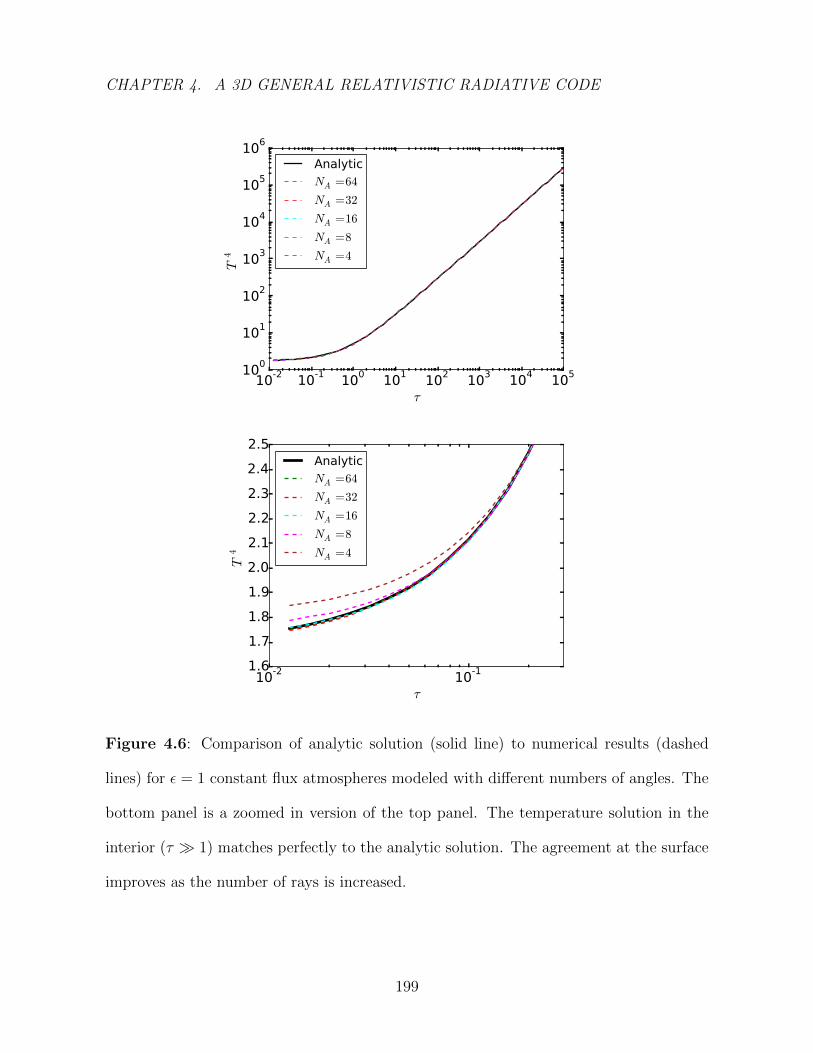
CHAPTER 4. A 3D GENERAL RELATIVISTIC RADIATIVE CODE
10-2 10-1 100 101 102 103 104 105
τ
100
101
102
103
104
105
106
T4
AnalyticNA =64
NA =32
NA =16
NA =8
NA =4
10-2 10-1
τ
1.61.71.81.92.02.12.22.32.42.5
T4
AnalyticNA =64
NA =32
NA =16
NA =8
NA =4
Figure 4.6: Comparison of analytic solution (solid line) to numerical results (dashed
lines) for ε = 1 constant flux atmospheres modeled with different numbers of angles. The
bottom panel is a zoomed in version of the top panel. The temperature solution in the
interior (τ 1) matches perfectly to the analytic solution. The agreement at the surface
improves as the number of rays is increased.
199
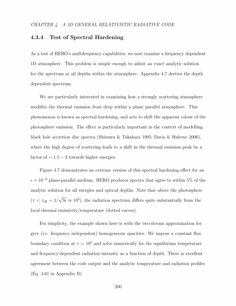
CHAPTER 4. A 3D GENERAL RELATIVISTIC RADIATIVE CODE
4.3.4 Test of Spectral Hardening
As a test of HERO’s multifrequency capabilities, we now examine a frequency dependent
1D atmosphere. This problem is simple enough to admit an exact analytic solution
for the spectrum at all depths within the atmosphere. Appendix 4.7 derives the depth
dependent spectrum.
We are particularly interested in examining how a strongly scattering atmosphere
modifies the thermal emission from deep within a plane parallel atmosphere. This
phenomenon is known as spectral hardening, and acts to shift the apparent colour of the
photosphere emission. The effect is particularly important in the context of modelling
black hole accretion disc spectra (Shimura & Takahara 1995; Davis & Hubeny 2006),
where the high degree of scattering leads to a shift in the thermal emission peak by a
factor of ∼ 1.5− 2 towards higher energies.
Figure 4.7 demonstrates an extreme version of this spectral hardening effect for an
ε = 10−6 plane-parallel medium. HERO produces spectra that agree to within 5% of the
analytic solution for all energies and optical depths. Note that above the photosphere
(τ < τeff = 1/√
3ε ≈ 103), the radiation spectrum differs quite substantially from the
local thermal emissivity/temperature (dotted curves).
For simplicity, the example shown here is with the two-stream approximation for
grey (i.e. frequency independent) homogeneous opacities. We impose a constant flux
boundary condition at τ = 105 and solve numerically for the equilibrium temperature
and frequency-dependent radiation intensity as a function of depth. There is excellent
agreement between the code output and the analytic temperature and radiation profiles
(Eq. 4.61 in Appendix B).
200

CHAPTER 4. A 3D GENERAL RELATIVISTIC RADIATIVE CODE
10-2 10-1 100 101 102
ν/T
10-5
10-4
10-3
10-2
10-1
100
101
102
103
Jν
τ=0
τ=1
τ=100
τ=10,000code Jν (τ)exact Jν (τ)Bν (τ)
Figure 4.7: Comparison of depth dependent spectra calculated using HERO (solid lines)
and the analytic solution (dashed lines) for a plane parallel thermal atmosphere. Note:
this is a highly scattering test problem with ε = 10−6, which results in significant spectral
hardening at the τ = 0 surface (compare dotted blue blackbody curve with solid blue
line). At all depths and frequencies, HERO is able to calculate the spectrum to within
5% of the true solution. The spatial resolution chosen for this calculation was 25 points
per decade in τ , and 20 points per decade in ν. The two-stream approximation was used
for handling angles (NA = 2).
4.3.5 Effect of a Heating Source
As a final accretion disc-like 1D test that utilizes most of the features of the code, we
discuss a problem that includes a heating source. We consider a slab with a total optical
depth of 2 × 10⁵ between two free surfaces. We assume grey opacities with ε = 10−4 (a
201

CHAPTER 4. A 3D GENERAL RELATIVISTIC RADIATIVE CODE
strongly scattering-dominated disc). The material in the slab is heated at a steady rate
of 10−5 (arbitrary units) per unit optical depth, so that the steady state flux from each
surface is unity. We use 20 angles and 61 frequencies.
We start the calculation with some arbitrary temperature profile (B = 104 at all τ
in this particular example) and we run HERO until it converges. After 3000 iterations
(this is many more than needed, but we wished to converge as much as possible for this
test), the radiative transfer equation has a maximum error of 10−6 and the radiative
equilibrium equation a maximum error of 10−7. The results are shown in Fig. 4.8. As
expected, the temperature profile is quadratic in τ and symmetric with respect to the
mid-plane (upper panel) and the radiation flux is linear in τ and antisymmetric (middle
panel). The lower panel shows spectra at various depths. In the deep interior of the
disc, the radiation is nearly blackbody, but as we approach the surface (τeff = τ√
3ε < 1)
there are signatures of spectral hardening. The radiation that escapes from the surface
is distinctly hardened.
202
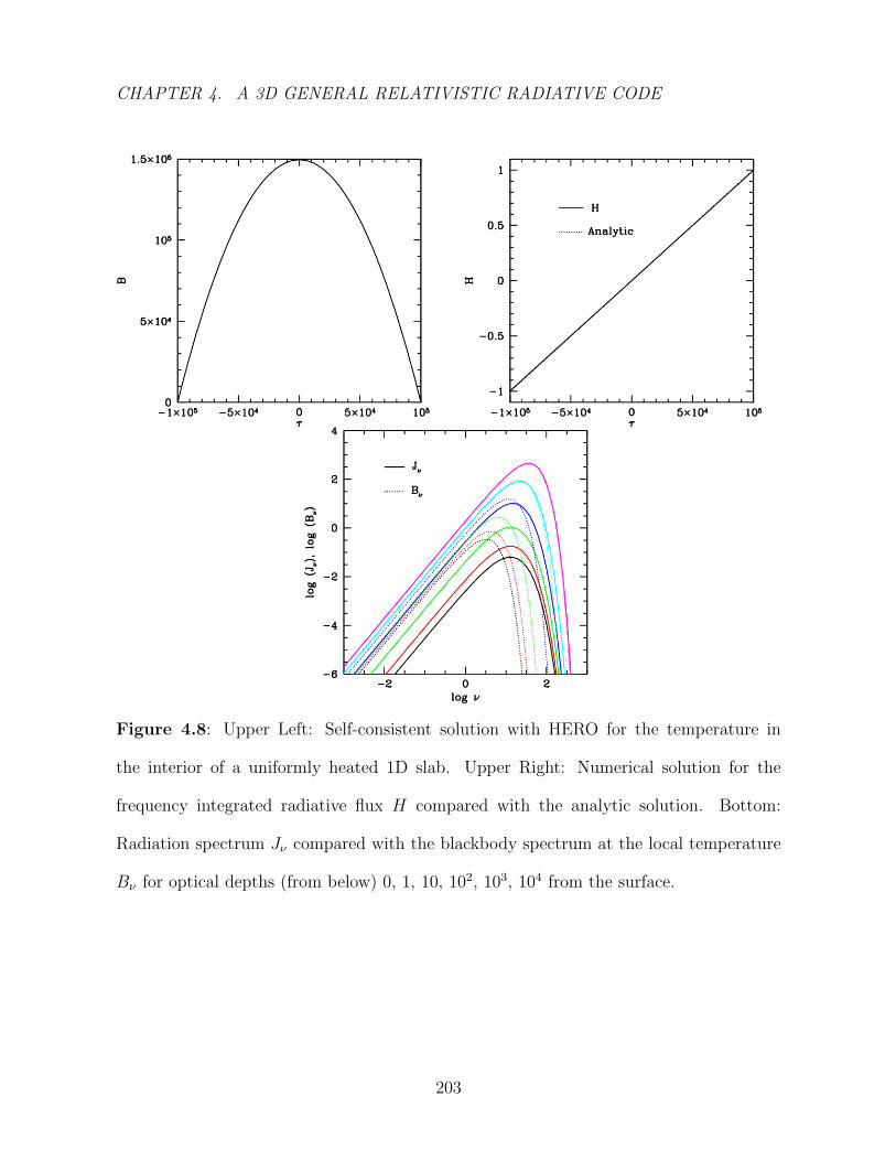
CHAPTER 4. A 3D GENERAL RELATIVISTIC RADIATIVE CODE
Figure 4.8: Upper Left: Self-consistent solution with HERO for the temperature in
the interior of a uniformly heated 1D slab. Upper Right: Numerical solution for the
frequency integrated radiative flux H compared with the analytic solution. Bottom:
Radiation spectrum Jν compared with the blackbody spectrum at the local temperature
Bν for optical depths (from below) 0, 1, 10, 102, 103, 104 from the surface.
203
CHAPTER 4. A 3D GENERAL RELATIVISTIC RADIATIVE CODE
4.3.6 2D Solutions and Ray Defects
A well known limitation of radiative solvers with discretized angular zones is the
appearance of “ray defects”. These are sharp linear features that arise because
interpolation on the angular grid is imperfect. The presence of ray defects is an
important motivator for us to use a hybrid scheme. Our long characteristics method
operates independently of an angular grid since it adaptively chooses an angular grid and
hence does not suffer from ray-defects. In the following sections, we compare our two
solvers, SC and LC, for a few test 2D problems. Appendix 4.6 provides a more extensive
discussion of the ray defects.
Opaque Wall Test
Ray-defects are particularly severe when there is a compact source of radiation (see
Fig. 4.18 in Appendix 4.6). But there are noticeable effects even in the case of smooth
extended sources. As an illustration, we analyze a simple 2D example where it is easy to
compute the exact solution. In the top panel of Figure 4.9, we show the radiation field
for an empty (zero opacity) box illuminated by a hot spot in the centre of the upper wall.
The boundary condition at this wall is an opaque (τ =∞) isotropic source function with
a gaussian profile:
S(x)
S(xc)= exp
[−(x− xc)2
w
], (4.41)
where xc corresponds to the centre of the box, and the width w is equal to 1/5 of the
box size. Since the interior of the box has no opacity, the radiation field at any point can
be easily found by tracing rays backwards and finding the source function corresponding
to the ray’s intersection point with the upper wall. We can thus calculate the mean
204
CHAPTER 4. A 3D GENERAL RELATIVISTIC RADIATIVE CODE
intensity J at every point inside the box.
In Figure 4.9, we compare the exact solution to the result from our two RT solvers.
For the SC solver (middle panel), a clear wave pattern appears along each of the angle
grid directions (we used NA = 20 in this test). These are the ray defects mentioned
earlier. The severity of the defects grows as we approach the upper wall, because of
the sharp break in the intensity distribution there. On the other hand, LC perfectly
reproduces the radiation pattern, even in the far field limit (compare top and bottom
panels of 4.9).
205

CHAPTER 4. A 3D GENERAL RELATIVISTIC RADIATIVE CODE
Figure 4.9: Comparison of radiation fields calculated using short and long characteristics
with an exact analytic solution for an opaque gaussian wall emitting into vacuum (colour
log J). From top to bottom: a) exact solution, b) SC solution (NA = 20), c) LC solution.
Note the appearance of systematic banding/waves in the SC case. These are ray defects.
206
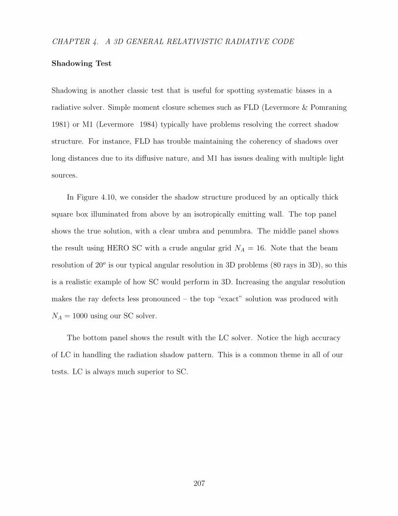
CHAPTER 4. A 3D GENERAL RELATIVISTIC RADIATIVE CODE
Shadowing Test
Shadowing is another classic test that is useful for spotting systematic biases in a
radiative solver. Simple moment closure schemes such as FLD (Levermore & Pomraning
1981) or M1 (Levermore 1984) typically have problems resolving the correct shadow
structure. For instance, FLD has trouble maintaining the coherency of shadows over
long distances due to its diffusive nature, and M1 has issues dealing with multiple light
sources.
In Figure 4.10, we consider the shadow structure produced by an optically thick
square box illuminated from above by an isotropically emitting wall. The top panel
shows the true solution, with a clear umbra and penumbra. The middle panel shows
the result using HERO SC with a crude angular grid NA = 16. Note that the beam
resolution of 20o is our typical angular resolution in 3D problems (80 rays in 3D), so this
is a realistic example of how SC would perform in 3D. Increasing the angular resolution
makes the ray defects less pronounced – the top “exact” solution was produced with
NA = 1000 using our SC solver.
The bottom panel shows the result with the LC solver. Notice the high accuracy
of LC in handling the radiation shadow pattern. This is a common theme in all of our
tests. LC is always much superior to SC.
207
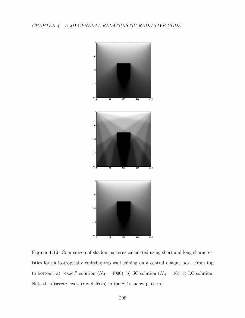
CHAPTER 4. A 3D GENERAL RELATIVISTIC RADIATIVE CODE
Figure 4.10: Comparison of shadow patterns calculated using short and long character-
istics for an isotropically emitting top wall shining on a central opaque box. From top
to bottom: a) “exact” solution (NA = 1000), b) SC solution (NA = 16), c) LC solution.
Note the discrete levels (ray defects) in the SC shadow pattern.
208
CHAPTER 4. A 3D GENERAL RELATIVISTIC RADIATIVE CODE
4.3.7 3D Solutions
We now shift our attention to 3D test problems, and begin by discussing ray-defects.
All the ray defects discussed in 2D (previous subsection and also Appendix 4.6) are
present in 3D as well, especially in the case of cartesian grids. A spherical polar grid (the
most natural choice for accretion problems) eliminates some problems by introducing
ray mixing via the curvilinear nature of the coordinate system. However, this is at the
expense of introducing a particularly serious defect for radial rays moving out from a
central source. Specifically, if one applies the SC method blindly on a spherical grid, one
will obtain a constant radiation energy density and flux at large radius instead of the
inverse square law fall-off one expects.
Dullemond & Turolla (2000) discuss a way to “fix” the radial beam problem. They
slightly modify the radiative transfer equation along the radial direction such that the
expected inverse-square falloff is recovered. We build on their suggestion, except that,
instead of modifying only one ray (the radial one), we treat all rays equally and apply an
artificial diffusion that, when coupled with a logarithmic radial grid, naturally produces
an inverse square falloff in the flux. Details of our diffusion method are explained in
Appendix §4.6.2. The following tests as well as those in §4.3.8 employ this ray diffusion
scheme.
Ring Benchmark
One particularly simple test problem is an axisymmetric opaque emitting ring in vacuum,
for which it is straightforward to calculate the radiation field at any point in space
analytically. For an infinitesimally thin ring emitting at the equatorial plane, the total
209
CHAPTER 4. A 3D GENERAL RELATIVISTIC RADIATIVE CODE
light reaching any position ~r is given by a 1-dimensional integral.
J(~r) =
∫C
|~r − ~rring(φ′)|2dφ′, (4.42)
where C is a constant specifying the emission per unit length of the ring. In spherical
coordinates, we have
J(r, θ, φ) =
∫C
r2 + r′2 − 2rr′ sin θ sin θ′ cos(φ− φ′)dφ′, (4.43)
where r′ = 0.5, θ′ = π/2, φ′ ∈ [0, 2π] are the coordinates of the ring in the setup
described here.
In Figure 4.11, we compare the results of SC and LC to the analytic result; the
constant C has been appropriately normalized to account for the finite emitting area
used in the LC/SC calculations. The LC calculation captures the radiation field perfectly
(δJ/J ≈ 10−3), whereas the SC result shows strong systematic ray-defect patterns. Note
that to enforce a 1/r2 falloff of the radiation field, the SC calculation employs our ray
diffusion scheme (otherwise, the result would be significantly worse).
210
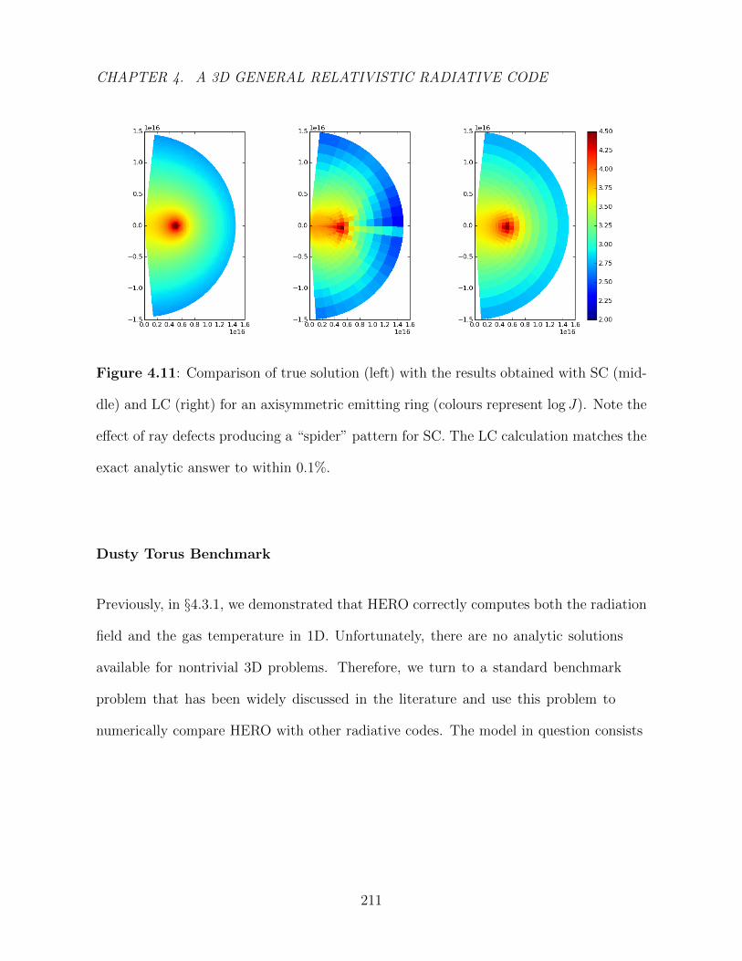
CHAPTER 4. A 3D GENERAL RELATIVISTIC RADIATIVE CODE
Figure 4.11: Comparison of true solution (left) with the results obtained with SC (mid-
dle) and LC (right) for an axisymmetric emitting ring (colours represent log J). Note the
effect of ray defects producing a “spider” pattern for SC. The LC calculation matches the
exact analytic answer to within 0.1%.
Dusty Torus Benchmark
Previously, in §4.3.1, we demonstrated that HERO correctly computes both the radiation
field and the gas temperature in 1D. Unfortunately, there are no analytic solutions
available for nontrivial 3D problems. Therefore, we turn to a standard benchmark
problem that has been widely discussed in the literature and use this problem to
numerically compare HERO with other radiative codes. The model in question consists
211
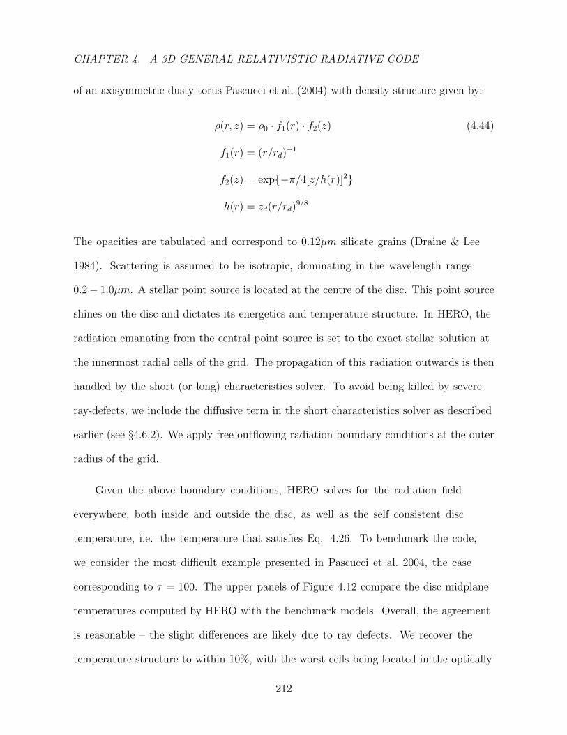
CHAPTER 4. A 3D GENERAL RELATIVISTIC RADIATIVE CODE
of an axisymmetric dusty torus Pascucci et al. (2004) with density structure given by:
ρ(r, z) = ρ0 · f1(r) · f2(z) (4.44)
f1(r) = (r/rd)−1
f2(z) = exp−π/4[z/h(r)]2
h(r) = zd(r/rd)9/8
The opacities are tabulated and correspond to 0.12µm silicate grains (Draine & Lee
1984). Scattering is assumed to be isotropic, dominating in the wavelength range
0.2− 1.0µm. A stellar point source is located at the centre of the disc. This point source
shines on the disc and dictates its energetics and temperature structure. In HERO, the
radiation emanating from the central point source is set to the exact stellar solution at
the innermost radial cells of the grid. The propagation of this radiation outwards is then
handled by the short (or long) characteristics solver. To avoid being killed by severe
ray-defects, we include the diffusive term in the short characteristics solver as described
earlier (see §4.6.2). We apply free outflowing radiation boundary conditions at the outer
radius of the grid.
Given the above boundary conditions, HERO solves for the radiation field
everywhere, both inside and outside the disc, as well as the self consistent disc
temperature, i.e. the temperature that satisfies Eq. 4.26. To benchmark the code,
we consider the most difficult example presented in Pascucci et al. 2004, the case
corresponding to τ = 100. The upper panels of Figure 4.12 compare the disc midplane
temperatures computed by HERO with the benchmark models. Overall, the agreement
is reasonable – the slight differences are likely due to ray defects. We recover the
temperature structure to within 10%, with the worst cells being located in the optically
212
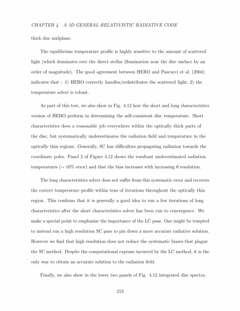
CHAPTER 4. A 3D GENERAL RELATIVISTIC RADIATIVE CODE
thick disc midplane.
The equilibrium temperature profile is highly sensitive to the amount of scattered
light (which dominates over the direct stellar illumination near the disc surface by an
order of magnitude). The good agreement between HERO and Pascucci et al. (2004)
indicates that : 1) HERO correctly handles/redistributes the scattered light; 2) the
temperature solver is robust.
As part of this test, we also show in Fig. 4.12 how the short and long characteristics
version of HERO perform in determining the self-consistent disc temperature. Short
characteristics does a reasonable job everywhere within the optically thick parts of
the disc, but systematically underestimates the radiation field and temperature in the
optically thin regions. Generally, SC has difficulties propagating radiation towards the
coordinate poles. Panel 2 of Figure 4.12 shows the resultant underestimated radiation
temperatures (∼ 10% error) and that the bias increases with increasing θ resolution.
The long characteristics solver does not suffer from this systematic error and recovers
the correct temperature profile within tens of iterations throughout the optically thin
region. This confirms that it is generally a good idea to run a few iterations of long
characteristics after the short characteristics solver has been run to convergence. We
make a special point to emphasize the importance of the LC pass. One might be tempted
to instead run a high resolution SC pass to pin down a more accurate radiative solution.
However we find that high resolution does not reduce the systematic biases that plague
the SC method. Despite the computational expense incurred by the LC method, it is the
only way to obtain an accurate solution to the radiation field.
Finally, we also show in the lower two panels of Fig. 4.12 integrated disc spectra.
213
CHAPTER 4. A 3D GENERAL RELATIVISTIC RADIATIVE CODE
Agreement between HERO and the other benchmark codes is within 20%, which is
comparable to the spread amongst the four independent codes discussed in Pascucci et
al. (2004). The HERO spectra were computed by raytracing from a distant observing
plane, making use of the complete radiative solution (i.e. Sν) obtained from our SC+LC
hybrid solver.
214
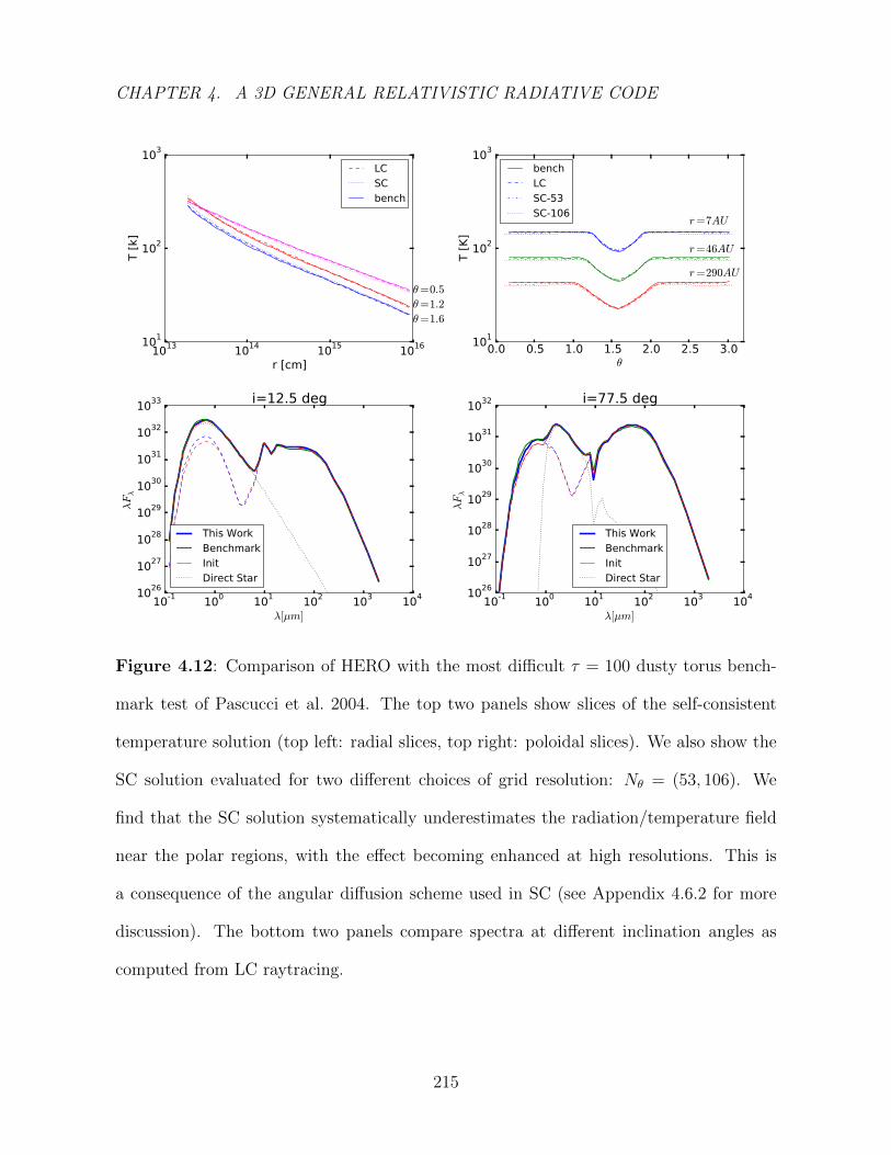
CHAPTER 4. A 3D GENERAL RELATIVISTIC RADIATIVE CODE
1013 1014 1015 1016
r [cm]
101
102
103
T [k
]
θ=0.5
θ=1.2
θ=1.6
LCSCbench
0.0 0.5 1.0 1.5 2.0 2.5 3.0θ
101
102
103
T [K
]
r=7AU
r=46AU
r=290AU
benchLCSC-53SC-106
10-1 100 101 102 103 104
λ[µm]
1026
1027
1028
1029
1030
1031
1032
1033
λFλ
i=12.5 deg
This WorkBenchmarkInitDirect Star
10-1 100 101 102 103 104
λ[µm]
1026
1027
1028
1029
1030
1031
1032
λFλ
i=77.5 deg
This WorkBenchmarkInitDirect Star
Figure 4.12: Comparison of HERO with the most difficult τ = 100 dusty torus bench-
mark test of Pascucci et al. 2004. The top two panels show slices of the self-consistent
temperature solution (top left: radial slices, top right: poloidal slices). We also show the
SC solution evaluated for two different choices of grid resolution: Nθ = (53, 106). We
find that the SC solution systematically underestimates the radiation/temperature field
near the polar regions, with the effect becoming enhanced at high resolutions. This is
a consequence of the angular diffusion scheme used in SC (see Appendix 4.6.2 for more
discussion). The bottom two panels compare spectra at different inclination angles as
computed from LC raytracing.
215
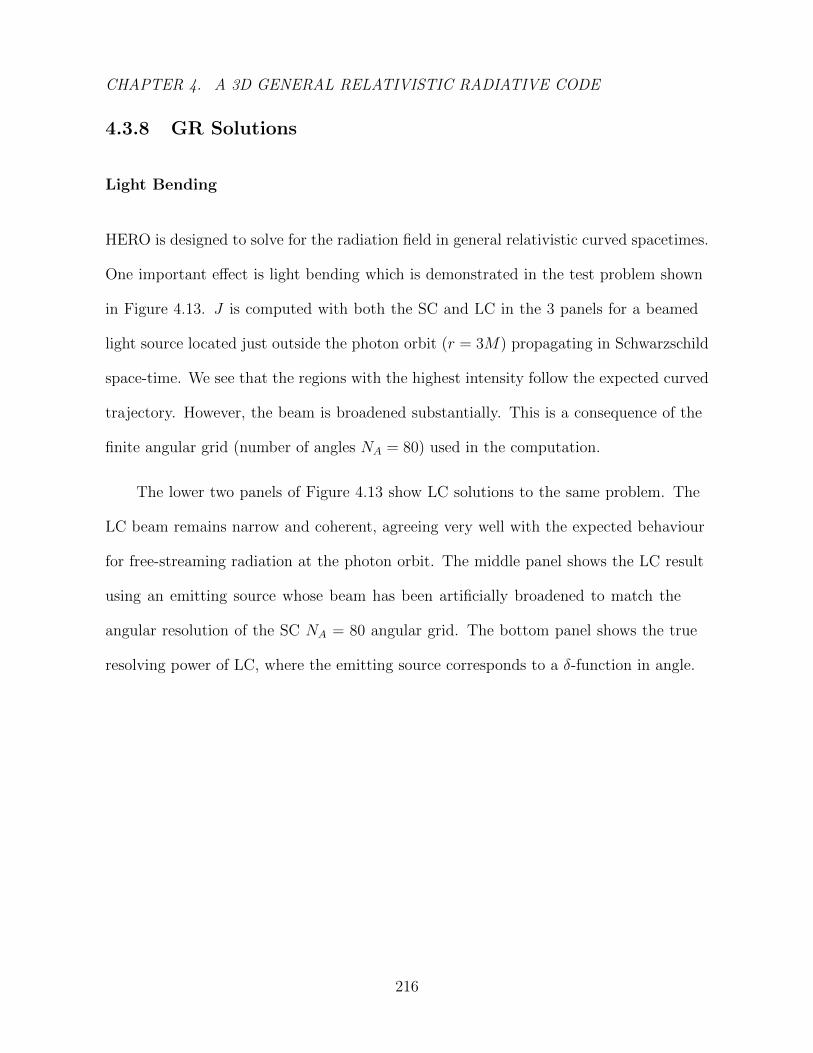
CHAPTER 4. A 3D GENERAL RELATIVISTIC RADIATIVE CODE
4.3.8 GR Solutions
Light Bending
HERO is designed to solve for the radiation field in general relativistic curved spacetimes.
One important effect is light bending which is demonstrated in the test problem shown
in Figure 4.13. J is computed with both the SC and LC in the 3 panels for a beamed
light source located just outside the photon orbit (r = 3M) propagating in Schwarzschild
space-time. We see that the regions with the highest intensity follow the expected curved
trajectory. However, the beam is broadened substantially. This is a consequence of the
finite angular grid (number of angles NA = 80) used in the computation.
The lower two panels of Figure 4.13 show LC solutions to the same problem. The
LC beam remains narrow and coherent, agreeing very well with the expected behaviour
for free-streaming radiation at the photon orbit. The middle panel shows the LC result
using an emitting source whose beam has been artificially broadened to match the
angular resolution of the SC NA = 80 angular grid. The bottom panel shows the true
resolving power of LC, where the emitting source corresponds to a δ-function in angle.
216

CHAPTER 4. A 3D GENERAL RELATIVISTIC RADIATIVE CODE
Figure 4.13: Light bending test for our two radiative solvers using a narrow laser beam
injected tangent to the r = 3 photon orbit. Upper left: SC, Upper right: LC with an
artificially broadened beam to match the SC angle grid size, Bottom: LC pure. The solid
black line shows the analytic result corresponding to the null geodesic.
217
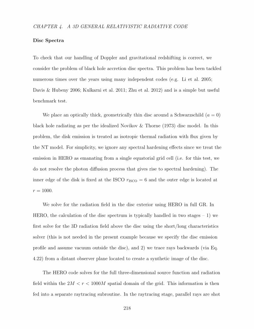
CHAPTER 4. A 3D GENERAL RELATIVISTIC RADIATIVE CODE
Disc Spectra
To check that our handling of Doppler and gravitational redshifting is correct, we
consider the problem of black hole accretion disc spectra. This problem has been tackled
numerous times over the years using many independent codes (e.g. Li et al. 2005;
Davis & Hubeny 2006; Kulkarni et al. 2011; Zhu et al. 2012) and is a simple but useful
benchmark test.
We place an optically thick, geometrically thin disc around a Schwarzschild (a = 0)
black hole radiating as per the idealized Novikov & Thorne (1973) disc model. In this
problem, the disk emission is treated as isotropic thermal radiation with flux given by
the NT model. For simplicity, we ignore any spectral hardening effects since we treat the
emission in HERO as emanating from a single equatorial grid cell (i.e. for this test, we
do not resolve the photon diffusion process that gives rise to spectral hardening). The
inner edge of the disk is fixed at the ISCO rISCO = 6 and the outer edge is located at
r = 1000.
We solve for the radiation field in the disc exterior using HERO in full GR. In
HERO, the calculation of the disc spectrum is typically handled in two stages – 1) we
first solve for the 3D radiation field above the disc using the short/long characteristics
solver (this is not needed in the present example because we specify the disc emission
profile and assume vacuum outside the disc), and 2) we trace rays backwards (via Eq.
4.22) from a distant observer plane located to create a synthetic image of the disc.
The HERO code solves for the full three-dimensional source function and radiation
field within the 2M < r < 1000M spatial domain of the grid. This information is then
fed into a separate raytracing subroutine. In the raytracing stage, parallel rays are shot
218

CHAPTER 4. A 3D GENERAL RELATIVISTIC RADIATIVE CODE
towards the disk distributed according to a squeezed logarithmic polar grid (the same
setup as Kulkarni et al. 2011) from an observer plane located at r = 100, 000M . The
final spectrum is generated by integrating the flux across the observer plane.
The top panel of Figure 4.14) shows the computed image for the particular example
problem. Integrating over this image yields the observed disc spectrum, which we show
in the lower panel. The disc spectrum computed with HERO agrees very well with a
previous calculation by Kulkarni et al. (2011), lending confidence that HERO correctly
handles GR effects.
219
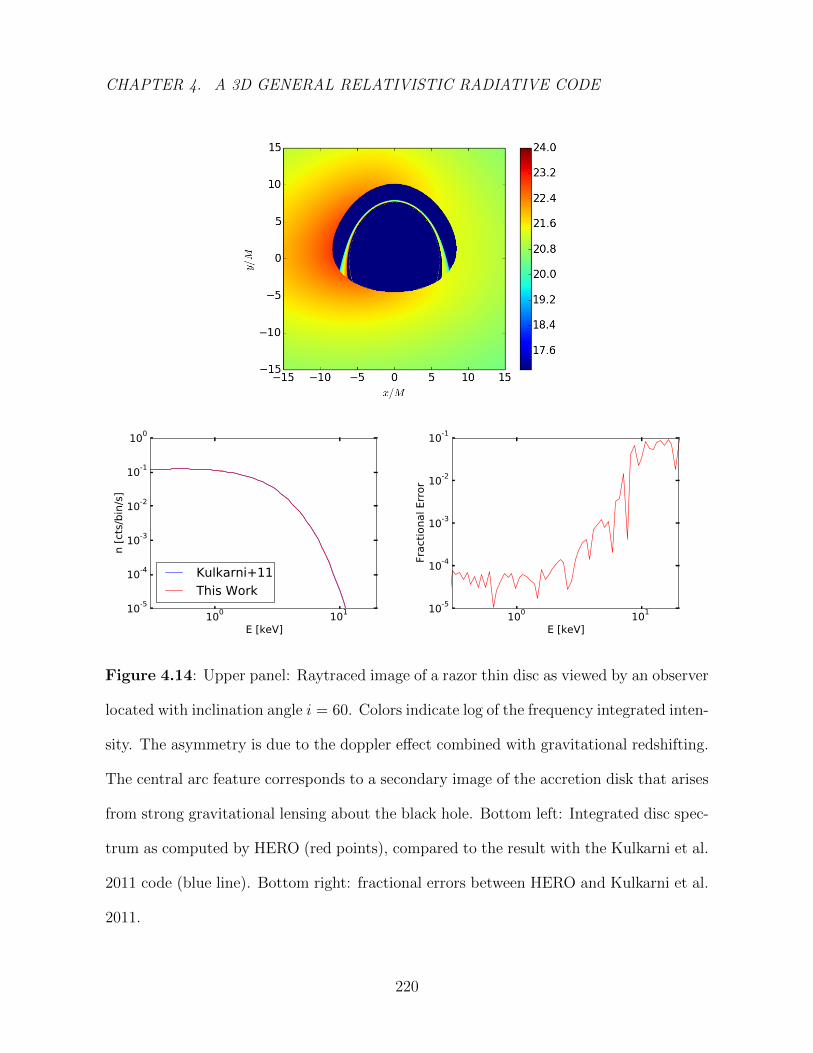
CHAPTER 4. A 3D GENERAL RELATIVISTIC RADIATIVE CODE
100 101
E [keV]
10-5
10-4
10-3
10-2
10-1
100
n [c
ts/b
in/s
]
Kulkarni+11This Work
100 101
E [keV]
10-5
10-4
10-3
10-2
10-1Fr
actio
nal E
rror
Figure 4.14: Upper panel: Raytraced image of a razor thin disc as viewed by an observer
located with inclination angle i = 60. Colors indicate log of the frequency integrated inten-
sity. The asymmetry is due to the doppler effect combined with gravitational redshifting.
The central arc feature corresponds to a secondary image of the accretion disk that arises
from strong gravitational lensing about the black hole. Bottom left: Integrated disc spec-
trum as computed by HERO (red points), compared to the result with the Kulkarni et al.
2011 code (blue line). Bottom right: fractional errors between HERO and Kulkarni et al.
2011.
220
CHAPTER 4. A 3D GENERAL RELATIVISTIC RADIATIVE CODE
Iron Line Spectra
In a similar vein as for the previous test, which was based on the NT continuum spectrum
of the disk, we also benchmark our code via a calculation of the emission profile due to a
monoenergetic line (e.g. Fe-Kα as seen in many Seyfert galaxies and some microquasars).
For a system that emits only monoenergetic δ-function lines, the final integrated line
profile depends only on the geometrical properties of the system (i.e. redshifting from
doppler/gravitational curvature and lensing effects from the Kerr metric).
We consider a Keplerian accretion disk in the Kerr metric whose line emission is
modulated by a power law emissivity profile F (r) ∝ r−3. We also set the domain of the
disk to span from rin = rISCO out to rout = 400. Figure 4.15 shows the resultant spectra
computed for two different choices of BH spin and two different choices of viewing angle.
We find good agreement between HERO and the benchmark code RELLINE (Dauser et
al. 2010, 2013), with the largest discrepancies occurring in the low energy red tail of the
line profiles.
The setup in HERO is identical to that of the previous NT disc tests, except that
a monoenergetic 6.4 keV line was used as the local emissivity instead of a thermal
continuum source. In addition, we use much higher resolution for the raytracing grid
since the low energy red tail of the line profile depends sensitively on how well the inner
edge of the disc is resolved.
221

CHAPTER 4. A 3D GENERAL RELATIVISTIC RADIATIVE CODE
0 2 4 6 8 10 12 14E [keV]
0.0
0.2
0.4
0.6
0.8
1.0
Phot
on C
ount
a=.998
a=0
i=30HERODauser+
0 2 4 6 8 10 12 14E [keV]
0.0
0.2
0.4
0.6
0.8
1.0
Phot
on C
ount
a=.998
a=0
i=60HERODauser+
Figure 4.15: A comparison of the Fe-Kα line profile as computed by HERO and
RELLINE (Dauser et al. 2013). Line profiles are computed for different viewing incli-
nations: top panel shows i = 30, whereas bottom panel shows i = 60.
222

CHAPTER 4. A 3D GENERAL RELATIVISTIC RADIATIVE CODE
Returning Radiation
Another classic accretion disk problem is that of computing the returning radiation due
to relativistic light bending around the black hole. For this test, we setup a razor thin
accretion disk that emits according to the standard thin disc luminosity profile (Page
& Thorne 1974) and measure the amount of returning radiation incident on the disk.
The goal is to benchmark both our SC and LC radiative solvers against the solutions
of Cunningham (1976), who tackled the same problem by means of relativistic transfer
functions.
In HERO, we model the returning radiation problem with a grey calculation (1
bolometric frequency bin) on an axisymmetric polar grid with (nr, nθ)=(60,30) restricted
to the upper half plane. The spatial grid was set as uniformly spaced in angle and log(r).
Boundary conditions invoked are: reflecting for the polar axis (to account for light that
passes through the pole), constant flux injection at the equatorial disk plane according
to (Page & Thorne 1974), and zero incident radiation at the inner and outer radial
boundaries.
In figure 4.16, we plot the incoming radiation flux at various locations above the disk
and compare to the solution of Cunningham (1976) for a moderately spinning a∗ = 0.9
black hole. We find that SC systematically overestimates the amount of returning flux
at large radii, presumably caused by the angular interpolation bleeding some of the
outbound radiation into inbound rays. LC on the other does not experience any strong
systematic biases, but suffers from a lack of resolving power at large radii since at these
large distances, the LC ray grid can miss the inner photon ring that is responsible for
most of the returning radiation.
223
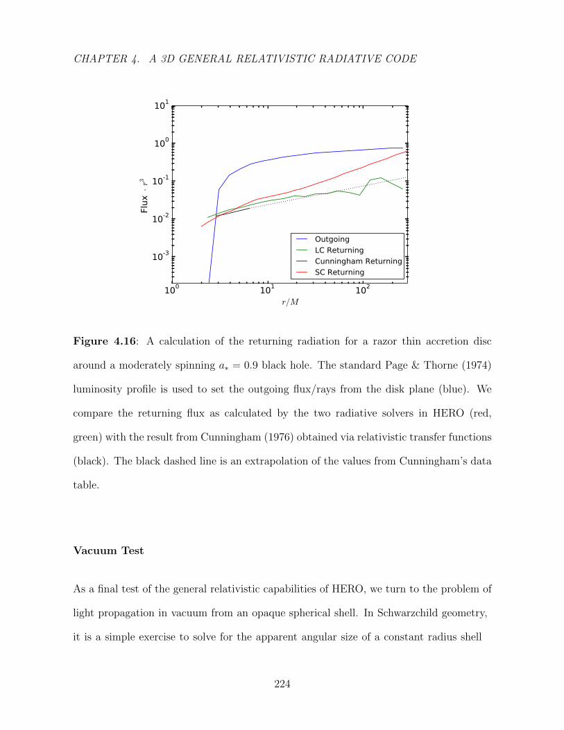
CHAPTER 4. A 3D GENERAL RELATIVISTIC RADIATIVE CODE
100 101 102
r/M
10-3
10-2
10-1
100
101
Flux
·r3
OutgoingLC ReturningCunningham ReturningSC Returning
Figure 4.16: A calculation of the returning radiation for a razor thin accretion disc
around a moderately spinning a∗ = 0.9 black hole. The standard Page & Thorne (1974)
luminosity profile is used to set the outgoing flux/rays from the disk plane (blue). We
compare the returning flux as calculated by the two radiative solvers in HERO (red,
green) with the result from Cunningham (1976) obtained via relativistic transfer functions
(black). The black dashed line is an extrapolation of the values from Cunningham’s data
table.
Vacuum Test
As a final test of the general relativistic capabilities of HERO, we turn to the problem of
light propagation in vacuum from an opaque spherical shell. In Schwarzchild geometry,
it is a simple exercise to solve for the apparent angular size of a constant radius shell
224
CHAPTER 4. A 3D GENERAL RELATIVISTIC RADIATIVE CODE
as viewed by an observer at some other (larger) radius. Furthermore, if the surface of
the shell radiates isotropically like a blackbody with a constant surface temperature, one
can calculate the radiation quantities (i.e. J, F, L) by simply integrating the constant
intensity across the apparent solid angle subtended by the shell. For instance, the radial
profile of luminosity has a particularly simple form, scaling directly with gravitational
redshift as
Llocal = L∞(1 + z)2 (4.45)
where Llocal = Flocal4πr2 is the total luminosity as measured by an observer at radius
r and L∞ is the luminosity at infinity. In Figure 4.17, we show the results for the
luminosity as calculated by our general-relativistic short and long characteristics solvers.
We normalize the luminosity by the redshift factors so the analytic solution simply
corresponds to a flat horizontal line (i.e., constant luminosity as measured at infinity).
In general, we find that our short characteristics solver systematically underestimates
the luminosity profile at large distances. These tests were carried out with the diffusion
prescription described earlier, therefore if the shell radiated purely in the radial direction,
SC would by construction give the correct answer. Here the surface radiates isotropically,
and there is a deviation from the true answer because of angle interpolation and diffusion.
The various SC curves in Figure 4.17 correspond to different choices for the radius of
the inner emitting shell. The high degree of similarity for all choices of inner radius
(i.e. ranging from from highly relativistic r0 = 3 in units of GM/c2 to nonrelativistic
r0 = 105) implies that the SC bias is independent of relativistic effects. It arises purely
from the discretization of the spatial and angular grid. While the bias is not negligible
– the luminosity is reduced by a factor of 2.5 at large radius – note that the luminosity
225

CHAPTER 4. A 3D GENERAL RELATIVISTIC RADIATIVE CODE
would be a factor ∼ 106 too large if we did not include diffusion. As with the other test
problems, LC gives an essentially perfect answer.
Panel two of Figure 4.17 shows another interesting phenomenon, viz., there is
a strong dependence between the SC bias on the choice of spatial grid resolution.
As we increase θ-resolution (keeping the r-resolution fixed), the luminosity profile of
our isotropically emitting shell exhibits a stronger bias to lower values. This effect is
ultimately caused by the angle diffusion scheme that we employ (c.f. Appendix 4.6.2).
The diffusion is tuned such that the radial cell-to-cell attenuation of light recovers the
inverse-square law. If the cell aspect ratio in r − θ is too rectangular, then the diffusion
has a strong directional preference. Light rays traveling along the short dimension of the
cell are overattenuated since they hit cell boundaries more often than rays traveling in
the long-dimension (the degree of diffusion is directly proportional to how often the light
ray traverses cells within a given spatial distance). Based on our tests, grid cells should
ideally have a square aspect ratio to minimize the error, and any ratio in excess of 2:1
should be avoided.
226

CHAPTER 4. A 3D GENERAL RELATIVISTIC RADIATIVE CODE
100 101 102 103
r/r0
10-2
10-1
100
L/(
1+z)
2 LC r0 =3
radialDullemondSC r0 =3
SC r0 =10
SC r0 =30
SC r0 =105
100 101 102 103
r/r0
10-1
100
L/(
1+z)
2
nθ =13
nθ =26
nθ =52
nθ =78
nθ =104
nθ =208
Figure 4.17: Variation in radial luminosity profiles as a function of a) relativistic effects
(lensing, redshifting) and b) grid-θ resolution. Note that the luminosity plotted is the
corrected luminosity as measured by an observer at infinity. The analytic solution is
therefore a constant L/(1 + z)2 for all radii.
227
CHAPTER 4. A 3D GENERAL RELATIVISTIC RADIATIVE CODE
4.4 Summary
We have described in this paper HERO, a new general relativistic radiative transfer code.
The primary aim of this code is to model the radiation field in accretion flows around
black holes. The unique features of HERO are: 1) a hybrid short/long characteristics
radiative solver that enables accurate and fast modelling of complex anisotropic radiation
fields; 2) implementation in a general relativistic framework taking into account the
effects of light bending, doppler beaming, and gravitational redshifting.
HERO is written as a post-processing code decoupled from the hydrodynamic
evolution of the fluid. It computes the time-independent radiation field assuming a
given fixed background fluid structure. Strictly speaking, this approach is valid only
for problems where the fluid velocities are small compared to the speed of light (i.e.
nonrelativistic flows). Alternatively, and this is the primary application we have in mind,
it could also be applied to time-steady relativistic problems.
We provide a detailed explanation of the long/short characteristics method used
to solve for the radiation field and our approach for solving the self-consistent gas
temperature. To verify that HERO produces physically correct answers, we have
performed a comprehensive set of tests designed to examine the code’s convergence
properties, accuracy, and capability to handle multidimensional relativistic problems.
We confirm the well known result that 2D and 3D problems with compact sources suffer
from significant ray defects in the far field when analyzed with the short characteristics
method. We present an approximate fix which mitigates the effects in the case of a
3D spherical grid. However, for accurate results, it is necessary to switch to a long
characteristics solver which is unaffected by ray-defects.
228

CHAPTER 4. A 3D GENERAL RELATIVISTIC RADIATIVE CODE
As the subject of a follow-up paper, we intend to apply HERO to radiative MHD
simulations of accretion discs – particularly simulations undergoing super-Eddington
accretion, where radiation feedback strongly dominates the dynamics of the flow. Using
HERO, we will investigate the integrated spectra to see the role that self-shadowing and
irradiation plays in these systems. This application requires a Comptonization module
which will be described in our next follow-up paper.
4.5 Acknowledgements
The authors would like to thank Nathan Roth, Jack Steiner, Jonathan McKinney,
James Guillonchon, Jeff McClintock, Yan-Fei Jiang, Javier Garcia, Eric Keto, and
Jiachen Jiang for their excellent insights on radiative transfer and comments/suggestions
regarding HERO. RN and YZ akcnowledge support from NSF grant AST1312651
and NASA grant NNX 14AB47G. AS acknowledges support for this work by NASA
through Einstein Post-doctoral Fellowships PF4-150126, awarded by the Chandra X-ray
Center, which is operated by the Smithsonian Astrophysical Observatory for NASA
under contract NAS8-03060. Finally, we are grateful for support from NSF XSEDE
grant TG-AST080026N, the NASA HEC Program, and the Harvard Odyssey cluster for
providing computing resources used in developing this code.
229
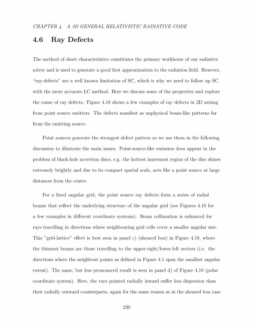
CHAPTER 4. A 3D GENERAL RELATIVISTIC RADIATIVE CODE
4.6 Ray Defects
The method of short characteristics constitutes the primary workhorse of our radiative
solver and is used to generate a good first approximation to the radiation field. However,
“ray-defects” are a well known limitation of SC, which is why we need to follow up SC
with the more accurate LC method. Here we discuss some of the properties and explore
the cause of ray defects. Figure 4.18 shows a few examples of ray defects in 2D arising
from point source emitters. The defects manifest as unphysical beam-like patterns far
from the emitting source.
Point sources generate the strongest defect pattern so we use them in the following
discussion to illustrate the main issues. Point-source-like emission does appear in the
problem of black-hole accretion discs, e.g. the hottest innermost region of the disc shines
extremely brightly and due to its compact spatial scale, acts like a point source at large
distances from the centre.
For a fixed angular grid, the point source ray defects form a series of radial
beams that reflect the underlying structure of the angular grid (see Figures 4.18 for
a few examples in different coordinate systems). Beam collimation is enhanced for
rays travelling in directions where neighbouring grid cells cover a smaller angular size.
This ”grid-lattice” effect is best seen in panel c) (sheared box) in Figure 4.18, where
the thinnest beams are those travelling to the upper-right/lower-left sectors (i.e. the
directions where the neighbour points as defined in Figure 4.1 span the smallest angular
extent). The same, but less pronounced result is seen in panel d) of Figure 4.18 (polar
coordinate system). Here, the rays pointed radially inward suffer less dispersion than
their radially outward counterparts, again for the same reason as in the sheared box case
230

CHAPTER 4. A 3D GENERAL RELATIVISTIC RADIATIVE CODE
(tighter angular packing occurs for the neighbour cells at smaller radius).
Finally, ray defects are particularly enhanced for rays that directly intersect
neighbouring cell centres (as an example, note that the 45o rays exhibit overwhelmingly
strong defect patterns in our cartesian setup in the top two panels of Fig 4.18).
Ideally, we would like to represent the discretized radiation pattern as a smooth field
instead of a superposition of laser beams. After much trial and error, we have arrived at
an angular diffusion based solution for spherical log polar grids. To motivate our final
solution, we first examine the root cause of the defects.
231
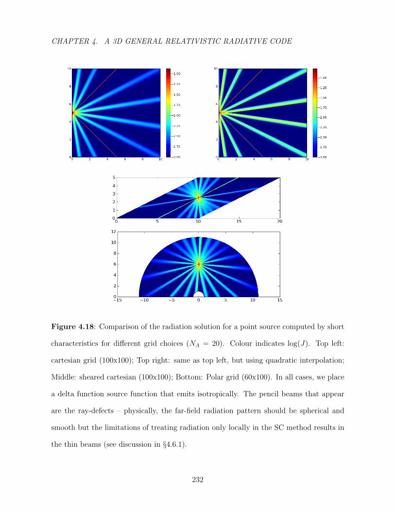
CHAPTER 4. A 3D GENERAL RELATIVISTIC RADIATIVE CODE
Figure 4.18: Comparison of the radiation solution for a point source computed by short
characteristics for different grid choices (NA = 20). Colour indicates log(J). Top left:
cartesian grid (100x100); Top right: same as top left, but using quadratic interpolation;
Middle: sheared cartesian (100x100); Bottom: Polar grid (60x100). In all cases, we place
a delta function source function that emits isotropically. The pencil beams that appear
are the ray-defects – physically, the far-field radiation pattern should be spherical and
smooth but the limitations of treating radiation only locally in the SC method results in
the thin beams (see discussion in §4.6.1).
232
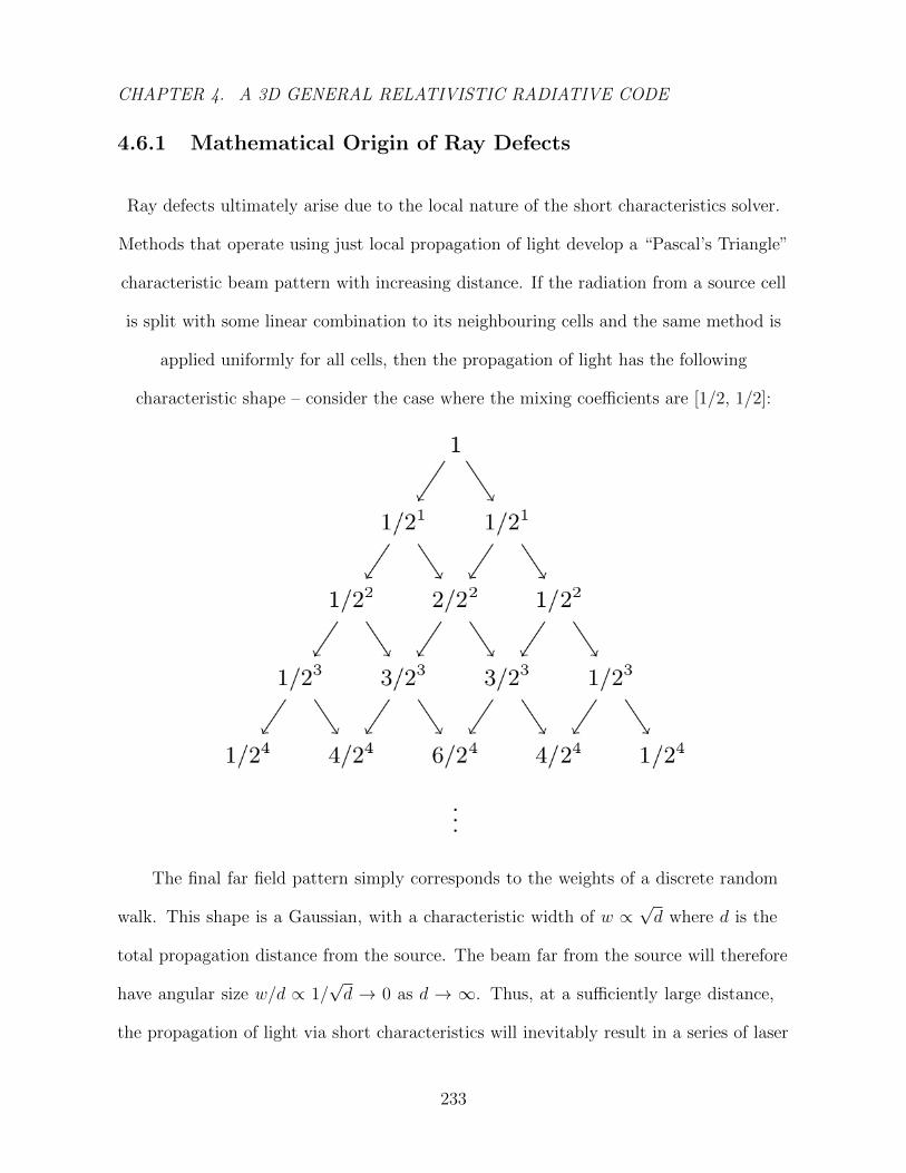
CHAPTER 4. A 3D GENERAL RELATIVISTIC RADIATIVE CODE
4.6.1 Mathematical Origin of Ray Defects
Ray defects ultimately arise due to the local nature of the short characteristics solver.
Methods that operate using just local propagation of light develop a “Pascal’s Triangle”
characteristic beam pattern with increasing distance. If the radiation from a source cell
is split with some linear combination to its neighbouring cells and the same method is
applied uniformly for all cells, then the propagation of light has the following
characteristic shape – consider the case where the mixing coefficients are [1/2, 1/2]:
The final far field pattern simply corresponds to the weights of a discrete random
walk. This shape is a Gaussian, with a characteristic width of w ∝√d where d is the
total propagation distance from the source. The beam far from the source will therefore
have angular size w/d ∝ 1/√d → 0 as d → ∞. Thus, at a sufficiently large distance,
the propagation of light via short characteristics will inevitably result in a series of laser
233
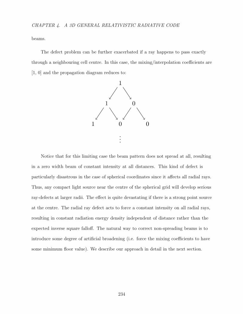
CHAPTER 4. A 3D GENERAL RELATIVISTIC RADIATIVE CODE
beams.
The defect problem can be further exacerbated if a ray happens to pass exactly
through a neighbouring cell centre. In this case, the mixing/interpolation coefficients are
[1, 0] and the propagation diagram reduces to:
Notice that for this limiting case the beam pattern does not spread at all, resulting
in a zero width beam of constant intensity at all distances. This kind of defect is
particularly disastrous in the case of spherical coordinates since it affects all radial rays.
Thus, any compact light source near the centre of the spherical grid will develop serious
ray-defects at larger radii. The effect is quite devastating if there is a strong point source
at the centre. The radial ray defect acts to force a constant intensity on all radial rays,
resulting in constant radiation energy density independent of distance rather than the
expected inverse square falloff. The natural way to correct non-spreading beams is to
introduce some degree of artificial broadening (i.e. force the mixing coefficients to have
some minimum floor value). We describe our approach in detail in the next section.
234

CHAPTER 4. A 3D GENERAL RELATIVISTIC RADIATIVE CODE
4.6.2 Ray Defect Correction Schemes
The most obvious approach to mitigate the impact of ray defects is simply increasing
the angular resolution. However this approach is not feasible for complex problems with
large spatial domains due to the unfavorable computational cost scaling with resolution.
One idea to combat ray defects is to use higher order interpolation schemes in
treating the propagation of radiation. Davis et al. (2012) found that quadratic monotonic
interpolation works well and suggest that it be used over standard linear interpolation.
Unfortunately, this does not address the fundamental problem of beam spreading –
higher order schemes are actually counterproductive in that they produce even thinner
beam patterns and amplify the significance of ray defects (Compare the top two panels
of Figure 4.18 for linear vs. quadratic interpolation) .
Ultimately, the problem (as illustrated in §4.6.1) has to do with the lack of spreading
for a single beam. This motivates us to implement a diffusive scheme to bring back the
necessary amount of spreading and to set the intensity values in such a way that an
inverse square falloff of radiation density and flux is recovered.
Our approach is the following: every time we read out intensity values from our
angular grid (i.e. the interpolation scheme described in §4.2.7), we apply a floor to our
interpolation coefficients so that there is always some degree of mixing between nearby
angles. That is, we modify the coefficients c1, c2, c3 in Eq. 4.39 to new values c′1, c′2, c′3
given by:
c′i =ci + w(∑i
ci
)+ 3w
(4.46)
where w is the diffusion coefficient that controls the amount of angle mixing. A more
235
CHAPTER 4. A 3D GENERAL RELATIVISTIC RADIATIVE CODE
physical way to understand this diffusion coefficient is to convert it into an attenuation
factor for nearby cells. For a monodirectional beam (i.e. I = 0 for all but a single angle
bin), the beam will attenuate by a factor a after propagating across a single cell, i.e.,
In+1 = aIn, (4.47)
where from Eq. 4.46, we find:
a = (1 + w)/(1 + 3w). (4.48)
This motivates a method for choosing the appropriate value of w for the case of a
log-polar grid (where the radial spacing is uniform in logr). Since we desire an inverse
square law falloff of the radiation field, we simply solve for a in the equation aNdec = 0.01
where Ndec is the number of cells per radial decade. For example if Ndec = 20 points per
decade (our canonical choice), we have have a = 0.794 and w = 0.149.
In Figure 4.19, we show radial profiles of F calculated with the SC for a point source
central star. Note that, in the absence of diffusion, the effect of radial ray defects is to
produce an unphysical solution where F is constant with radius.
In Figure 4.20, we show the results from this diffusion scheme compared to the
exact solution for an off-centre equatorial ring source (e.g. the same setup as described
in §4.3.7) for different choices of the spatial grid resolution. We find that our diffusive
scheme suffers from systematic overattentuation in the polar regions for spatial grids
that too rectangular. We recommend keeping the grid cell aspect ratio as close to square
(1:1) as possible in order to minimize this effect.
The scheme described here is a generalization of that proposed by Dullemond &
Turolla 2000. They applied the same factor a derived above except that they did it
236

CHAPTER 4. A 3D GENERAL RELATIVISTIC RADIATIVE CODE
solely for the radial ray. For a central point source, which produces only radial rays,
their method and ours produce the same correct inverse-law behaviour of flux. However,
when the source is extended, e.g., the spherical shell test problem described in §4.3.8,
their method causes the intensity to fall too steeply. Our method also suffers a similar
systematic bias, but it is less severe (see Fig. 4.17). In the limit of an isotropic radiation
field, e.g., the interior of a blackbody enclosure, their method would still cause intensity
to decline with increasing radius. Our diffusive method, on the other hand, would give
the correct result, viz., no change in intensity. These differences are relatively minor.
The main feature of both approaches is that they recover the inverse square law at least
approximately. However, a major limitation of our diffusive approach is that it only
works for the case of uniform log-radial grids.
1013 1014 1015 1016 1017
r [cm]
10-7
10-6
10-5
10-4
10-3
10-2
10-1
100
F/F
0
w=0
w=0.1
w=0.149
w=0.2
r−2
Figure 4.19: Radial profiles of F for various choices of diffusion coefficient as calculated
by short characteristics code on a spherical polar grid (nr, nθ) = (60, 100). Given these
grid dimensions, the diffusion coefficient must be set to w = 0.149 in order to reproduce
an inverse square falloff for flux.
237

CHAPTER 4. A 3D GENERAL RELATIVISTIC RADIATIVE CODE
Figure 4.20: Ray defect pattern from an isotropically emitting ring for 3 different choices
of grid resolution. Here we use a spherical spatial grid with locally defined ray angles.
Panels: a) (nθ = 26) square aspect ratio; b) (nθ = 52) 1:2 aspect ratio; c) (nθ = 104) 1:4
aspect ratio. Notice the systematic reduction of radiation near the polar regions when nθ
increases and also the characteristic “spider” pattern arising from our choice of spatial
grid interpolation.
4.7 Analytic 1D Atmosphere Spectrum
In this problem, we set up a constant flux 1D atmosphere subject to fixed grey
opacities (κν = const) with an absorption fraction set to ε = 10−6 (i.e. a highly
scattering-dominated atmosphere). The local source function is a combination of thermal
emission and reflected light (c.f. Eq 4.6).
The analytic solution to this problem can be easily obtained by considering the
238
CHAPTER 4. A 3D GENERAL RELATIVISTIC RADIATIVE CODE
moments of the radiative transfer equation. We define the first few moments of the
intensity field as
Jν =1
2
1∫−1
Iνdµ,
Hν =1
2
1∫−1
µIνdµ,
Kν =1
2
1∫−1
µ2Iνdµ, (4.49)
where µ ≡ cos(θ) is the angle cosine with respect to the plane normal. Using these
quantities allows us to write the moments of the radiative transfer equation as:
dHν
dτν= ε(Jν −Bν) (4.50)
dKν
dτν= Hν (4.51)
Combining Eqs. 4.50 + 4.51 and invoking the Eddington approximation (Kν = Jν/3)
yields
d2Jνdτ 2
ν
= 3ε(Jν −Bν), (4.52)
which is simply a constant coefficient second-order inhomogeneous differential equation
in Jν . This allows us to construct an exact solution using standard methods. The
solutions to the homogeneous system are simply
φ1(τ) = exp(√
3ετ),
φ2(τ) = exp(−√
3ετ). (4.53)
239
CHAPTER 4. A 3D GENERAL RELATIVISTIC RADIATIVE CODE
The particular solution Jp that satisfies the inhomogeneous system is given by3
Jp(τ) = φ1(τ)
∞∫τ
φ2g
Wdτ ′ + φ2(τ)
τ∫0
φ1g
Wdτ ′, (4.54)
where g = 3εB is the inhomogeneous function, and W denotes the Wronskian, defined by
W ≡ dφ1
dτφ2 −
dφ2
dτφ1 (4.55)
= 2√
3ε (4.56)
Putting everything together, the solution takes the form
J = Jp + c1φ1 + c2φ2, (4.57)
where the undetermined constants are set by the boundary conditions of the problem.
At the τ →∞ inner boundary we expect J → B, so we must eliminate the exponentially
growing mode by setting c1 = 0. To set the surface boundary condition, we make use of
the two-stream approximation and evaluate
H(τ) =1√3
dJ
dτ(4.58)
and enforce a surface boundary condition that is consistent with the Eddington
approximation:
H(0)
J(0)=
1√3, (4.59)
which sets
c2 = −
(1−√
3
1 +√
3
)φ2
∞∫0
φ2g
Wdτ ′. (4.60)
The final step is to determine the thermal source (B(τ)) that is consistent with our
radiation solution from Eq. 4.57. This can be calculated using our two radiative transfer
3The particular solution is constructed via the “variation of parameters” method
240

CHAPTER 4. A 3D GENERAL RELATIVISTIC RADIATIVE CODE
moment equations. Since we have a constant flux atmosphere, dH/dτ = 0, which implies
J(τ) = B(τ) from Eq. 4.50. We combine this with integrating the pressure equation
(Eq. 4.51) to yield the full solution
J(τ) = 3Hτ + J(0)
→ B(τ) = 3H
(τ +
1√3
)(4.61)
241
Chapter 5
HEROIC - A Comptonization
Module for the HERO radiative code
This thesis chapter will be submitted to MNRAS
Y. Zhu, R. Narayan, D. Psaltis, A. Sadowski, in prep
Abstract
We describe HEROIC, an upgrade of the relativistic radiative code HERO which now
Includes Comptonization. To model the Comptonization process, we employ a quadratic
Kompaneets operator approach to handle the photon energy redistribution process.
We benchmark and test our code with simple 1D and 3D scattering problems that
admit analytic solutions. We then apply HEROIC to the astrophysical problem of a
scattering-dominated hot accretion disk. We find that our 3D calculation yields slightly
hotter spectra than previous 1D-based estimates. We also find a high energy power-law
242
CHAPTER 5. 3D COMPTONIZED ACCRETION DISKS
tail that is sourced by the hot thermal emission from the plunging region of the disk.
5.1 Introduction
Comptonization plays a crucial role in determining the high-energy emission properties
of a huge variety of astrophysical objects, such as the X-ray radiation from the nuclei
of galaxies/quasars (Veledina, Vurm, & Poutanen 2011), governing the decay rates of
neutron star bursters (Joss 1977; Lamb et al. 1977), the light passing through plasma
clouds of the intra-cluster medium (Prokhorov et al. 2010), and nonthermal spectral
properties of galactic microquasars (McClintock & Remillard 2006). The ubiquity of
hot ionized gas in astrophysical settings motivates the need for accurate treatment and
modelling of the Compton scattering process.
In the case of black hole accretion disks, cold seed photons emitted from a thermal
disk get upscattered by hot coronal electrons (Sunyaev & Titarchuk 1980), producing a
whole host of spectral shapes in X-rays such as power-laws and Compton humps. Many
systems, especially those in the low-hard spectral state, are observed with a dominant
Compton component (Zdziarski et al. 1995; Gierlinski et al. 1997), where interpretation
of the data requires accurate modeling of the power-law tail. This is especially true in
the case of reflection line modeling for black hole systems (Fabian et al. 1989; Tanaka et
al. 1995; Miller 2007), where slight errors in the continuum can lead to large systematic
biases in the derived black hole parameters (Weaver, Krolik & Pier 1998; Miller et al.
2006; Kolehmainen & Done 2010; Kolehmainen, Done & Diaz Trigo 2014).
Accurate analytic models of the Comptonized spectrum have been worked out
243
CHAPTER 5. 3D COMPTONIZED ACCRETION DISKS
several decades ago for various regimes such as for optically thick, homogeneous 1D and
3D media (Sunyaev & Titarchuk 1980), the limit of low electron energies (Titarchuk &
Hua 1995), or the relativistic limit for an optically thin medium (Coppi 1991). However,
the complex nature of accretion flows around black holes precludes the use of analytic
models, motivating the development of numerical Comptonization schemes.
Monte-Carlo based methods are by far the most popular approach to the problem
(Pozdnyakov, Sobol, Sunyaev 1983; Gorecki & Wilczewski 1984; Stern et al. 1995;
Malzac & Jourdain 2000; Schnittman & Krolik 2013) owing to the ease with which
the technique can handle relativistic geometries and the complex angle and frequency
dependent scattering process. The biggest drawback of the Monte-Carlo (MC) approach
is that photon statistics limit the accuracy of the computations, posing difficulties in
generating spectral models for data fitting since the results differ each time the code
is run. This problem is worst in the limit of extreme photon energies, where there is a
dearth of photons and hence poor photon statistics 1. MC methods also suffer in the
limit of high optical depths – here, the full photon diffusion process is incredibly taxing
computationally, which in practice restricts MC based codes to problems with only
moderate optical depths (i.e. τ . 10).
Another approach is to discretize the problem and numerically solve the radiative
transfer problem for some preset fixed geometry (e.g. compPS: Poutanen & Svensson
1996 for moderate optical depths; compTT: Titarchuk & Lyubarskij 1995 for accretion
disks; TLUSTY: for 1D atmospheres Hubeny et al. 2001). The main advantage of this
1The use of an energy-weighted scattering kernel is one work-around for the photon-starvation problem
in MC methods.
244
CHAPTER 5. 3D COMPTONIZED ACCRETION DISKS
approach is that it can easily handle optically thick problems via a Kompaneets operator
approach (Kompaneets 1957), which uses a diffusion approximation to handle the
nonrelativistic Comptonization problem. This approach is particularly amenable to the
short characteristics fixed-grid framework of HERO, our 3D GR radiation postprocessor
code (see Chapter 4). In this work, we implement Comptonization in our code and
update the name to HEROIC (HERO Including Comptonization). The primary advance
in our work is that we introduce a fully self-consistent relativistic radiation module for
the 3D Comptonization problem of hot accretion flows around black holes.
Regardless of the approach taken for solving the Compton problem, a final
raytracing calculation is needed to connect the result to the actual spectral observations
of astrophysical systems. Typically, geodesic paths are traced backwards from a distant
observation plane until they hit the accretion flow (e.g. see Rauch & Blandford 1994;
Broderick & Blandford 2003; Dovciak et al. 2004; Dexter & Agol 2009; Johannsen &
Psaltis 2010; Kulkarni et al. 2011; Zhu et al. 2012). This yields a transfer function that
allows one to map the local Comptonized disk emission to the spectrum as measured
by the distant observer. In cases of high scattering optical depths, it is crucial for
raytracing methods to resolve the complete nonlocal structure of the scattered radiation
field (Schnittman & Krolik 2013). For MC-based methods, this translates to a more
computationally expensive “emitter-to-observer” paradigm since this is how the photon
diffusion process works in nature (see Laor et al. 1990; Kojima 1991; Dolence et al. 2009;
Schnittman & Krolik 2013 for a few recent codes that follow this philosophy). Grid based
methods instead require a fully 3D treatment of the radiative problem accounting for all
the nonlocal scattering terms in the emissivity profile. In the case of HEROIC, this is
achieved by solving for the complete 3D scattered radiation field everywhere around and
245
CHAPTER 5. 3D COMPTONIZED ACCRETION DISKS
inside the disk before the raytracing process is initiated.
The organization of this paper is as follows: in §5.2 we describe how HEROIC
handles Comptonization; specifically, we explain how the ray evolution equation works
in accordance to the Kompaneets based approach that we have taken. §5.3 follows up
with a series of 1D and 3D benchmark tests to verify the correct operation of our code.
Finally, we present in §5.4 an application of HEROIC to a couple of general relativistic
magnetohydrodynamic (GRMHD) disk simulations. We find that the GRMHD based
3D spectra are slightly hotter than previous 1D estimates.
5.2 Radiative Transfer Solution
The approach HEROIC uses for solving radiative transfer is the method of characteristics
(see Chapter 4 for an extensive discussion). The intensity field is evolved along a set of
discrete rays according to the radiative transfer equation:
dI
dτ= −I + S, (5.1)
where I is the radiation intensity along the ray, τ is the optical depth, and S is the
source function that governs the rate at which energy is reintroduced back into the beam,
accounting for both intrinsic thermal emission and scattering. Specifically, we use
S =αB + σJ
α + σ, (5.2)
where α and σ are the absorption and scattering opacities respectively, B is the thermal
Planck function, and J is the radiation mean intensity averaged over 4π solid angle.
Notice the implicit coupling between the source function and the radiative transfer
equation. Ray intensities are updated according to the local spatially varying source
246
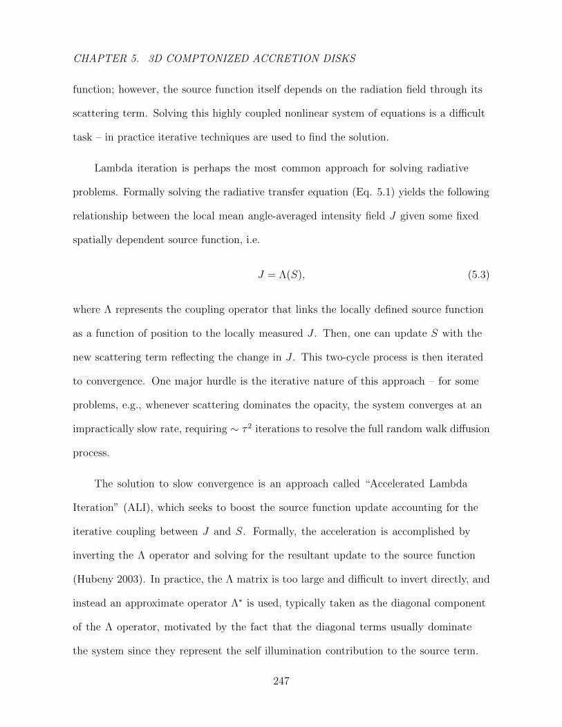
CHAPTER 5. 3D COMPTONIZED ACCRETION DISKS
function; however, the source function itself depends on the radiation field through its
scattering term. Solving this highly coupled nonlinear system of equations is a difficult
task – in practice iterative techniques are used to find the solution.
Lambda iteration is perhaps the most common approach for solving radiative
problems. Formally solving the radiative transfer equation (Eq. 5.1) yields the following
relationship between the local mean angle-averaged intensity field J given some fixed
spatially dependent source function, i.e.
J = Λ(S), (5.3)
where Λ represents the coupling operator that links the locally defined source function
as a function of position to the locally measured J . Then, one can update S with the
new scattering term reflecting the change in J . This two-cycle process is then iterated
to convergence. One major hurdle is the iterative nature of this approach – for some
problems, e.g., whenever scattering dominates the opacity, the system converges at an
impractically slow rate, requiring ∼ τ 2 iterations to resolve the full random walk diffusion
process.
The solution to slow convergence is an approach called “Accelerated Lambda
Iteration” (ALI), which seeks to boost the source function update accounting for the
iterative coupling between J and S. Formally, the acceleration is accomplished by
inverting the Λ operator and solving for the resultant update to the source function
(Hubeny 2003). In practice, the Λ matrix is too large and difficult to invert directly, and
instead an approximate operator Λ∗ is used, typically taken as the diagonal component
of the Λ operator, motivated by the fact that the diagonal terms usually dominate
the system since they represent the self illumination contribution to the source term.
247
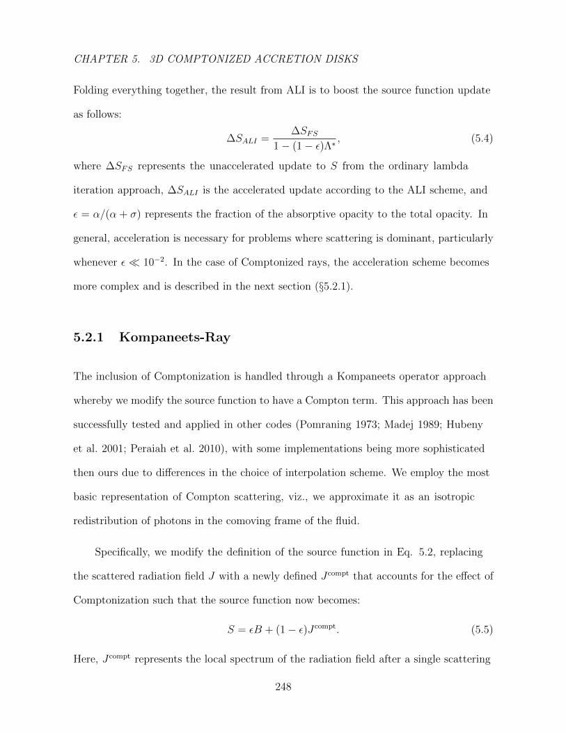
CHAPTER 5. 3D COMPTONIZED ACCRETION DISKS
Folding everything together, the result from ALI is to boost the source function update
as follows:
∆SALI =∆SFS
1− (1− ε)Λ∗, (5.4)
where ∆SFS represents the unaccelerated update to S from the ordinary lambda
iteration approach, ∆SALI is the accelerated update according to the ALI scheme, and
ε = α/(α + σ) represents the fraction of the absorptive opacity to the total opacity. In
general, acceleration is necessary for problems where scattering is dominant, particularly
whenever ε 10−2. In the case of Comptonized rays, the acceleration scheme becomes
more complex and is described in the next section (§5.2.1).
5.2.1 Kompaneets-Ray
The inclusion of Comptonization is handled through a Kompaneets operator approach
whereby we modify the source function to have a Compton term. This approach has been
successfully tested and applied in other codes (Pomraning 1973; Madej 1989; Hubeny
et al. 2001; Peraiah et al. 2010), with some implementations being more sophisticated
then ours due to differences in the choice of interpolation scheme. We employ the most
basic representation of Compton scattering, viz., we approximate it as an isotropic
redistribution of photons in the comoving frame of the fluid.
Specifically, we modify the definition of the source function in Eq. 5.2, replacing
the scattered radiation field J with a newly defined Jcompt that accounts for the effect of
Comptonization such that the source function now becomes:
S = εB + (1− ε)Jcompt. (5.5)
Here, Jcompt represents the local spectrum of the radiation field after a single scattering
248
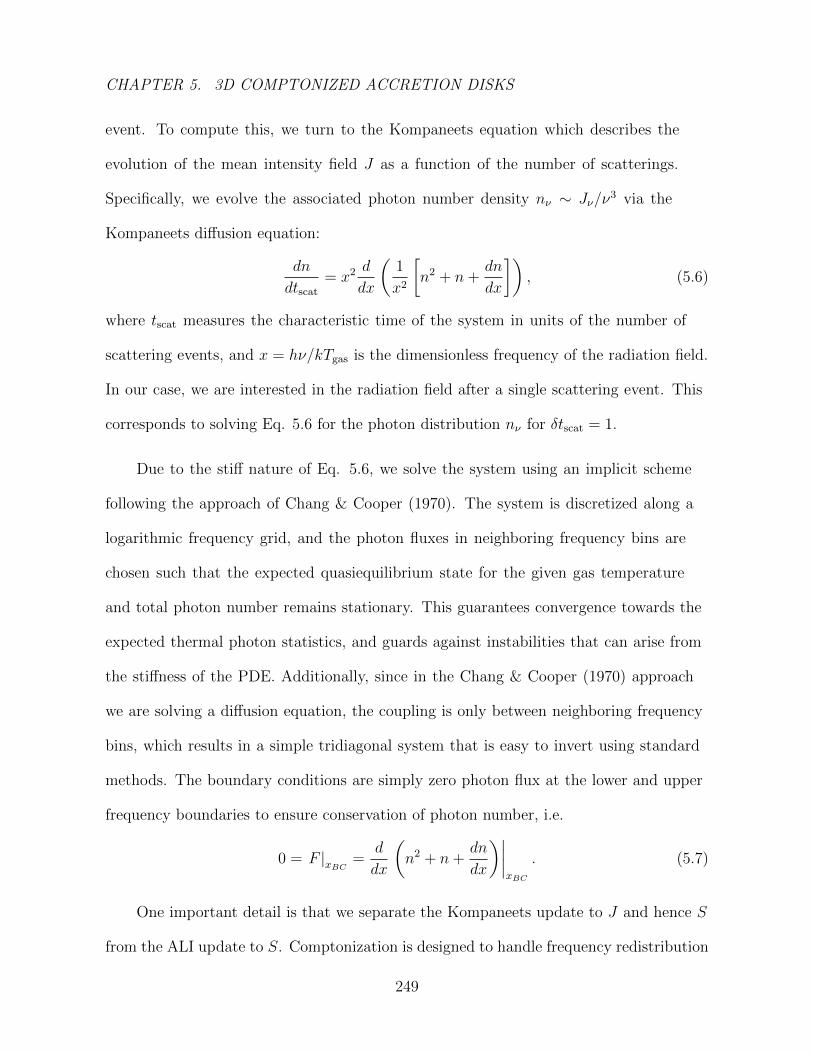
CHAPTER 5. 3D COMPTONIZED ACCRETION DISKS
event. To compute this, we turn to the Kompaneets equation which describes the
evolution of the mean intensity field J as a function of the number of scatterings.
Specifically, we evolve the associated photon number density nν ∼ Jν/ν3 via the
Kompaneets diffusion equation:
dn
dtscat
= x2 d
dx
(1
x2
[n2 + n+
dn
dx
]), (5.6)
where tscat measures the characteristic time of the system in units of the number of
scattering events, and x = hν/kTgas is the dimensionless frequency of the radiation field.
In our case, we are interested in the radiation field after a single scattering event. This
corresponds to solving Eq. 5.6 for the photon distribution nν for δtscat = 1.
Due to the stiff nature of Eq. 5.6, we solve the system using an implicit scheme
following the approach of Chang & Cooper (1970). The system is discretized along a
logarithmic frequency grid, and the photon fluxes in neighboring frequency bins are
chosen such that the expected quasiequilibrium state for the given gas temperature
and total photon number remains stationary. This guarantees convergence towards the
expected thermal photon statistics, and guards against instabilities that can arise from
the stiffness of the PDE. Additionally, since in the Chang & Cooper (1970) approach
we are solving a diffusion equation, the coupling is only between neighboring frequency
bins, which results in a simple tridiagonal system that is easy to invert using standard
methods. The boundary conditions are simply zero photon flux at the lower and upper
frequency boundaries to ensure conservation of photon number, i.e.
0 = F |xBC=
d
dx
(n2 + n+
dn
dx
)∣∣∣∣xBC
. (5.7)
One important detail is that we separate the Kompaneets update to J and hence S
from the ALI update to S. Comptonization is designed to handle frequency redistribution
249
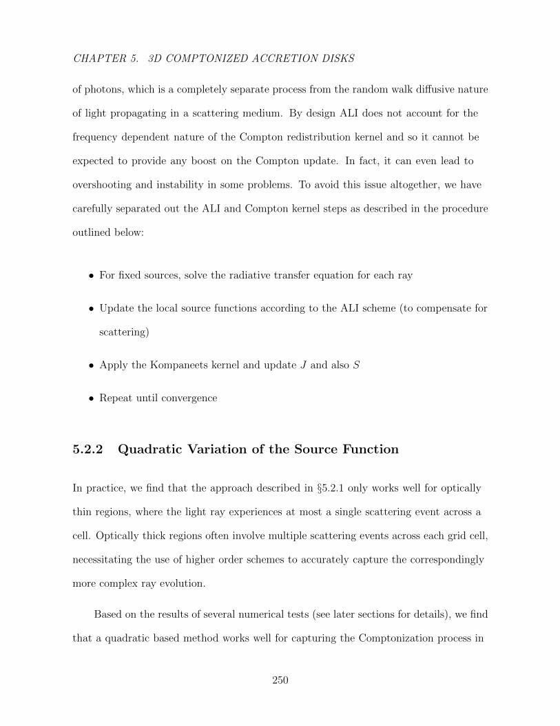
CHAPTER 5. 3D COMPTONIZED ACCRETION DISKS
of photons, which is a completely separate process from the random walk diffusive nature
of light propagating in a scattering medium. By design ALI does not account for the
frequency dependent nature of the Compton redistribution kernel and so it cannot be
expected to provide any boost on the Compton update. In fact, it can even lead to
overshooting and instability in some problems. To avoid this issue altogether, we have
carefully separated out the ALI and Compton kernel steps as described in the procedure
outlined below:
• For fixed sources, solve the radiative transfer equation for each ray
• Update the local source functions according to the ALI scheme (to compensate for
scattering)
• Apply the Kompaneets kernel and update J and also S
• Repeat until convergence
5.2.2 Quadratic Variation of the Source Function
In practice, we find that the approach described in §5.2.1 only works well for optically
thin regions, where the light ray experiences at most a single scattering event across a
cell. Optically thick regions often involve multiple scattering events across each grid cell,
necessitating the use of higher order schemes to accurately capture the correspondingly
more complex ray evolution.
Based on the results of several numerical tests (see later sections for details), we find
that a quadratic based method works well for capturing the Comptonization process in
250
CHAPTER 5. 3D COMPTONIZED ACCRETION DISKS
the limit of optically thick cells. When evaluating the formal solution to the radiative
transfer equation, i.e. the solution to
I(τ) = I0e−τ +
∫ τ
0
S(τ ′) exp(−τ ′)dτ ′, (5.8)
we choose to approximate S(τ) with a quadratic Taylor-series decomposition:
S(τ) = S(τ0) +dS
dτ(τ − τ0) +
1
2
(d2S
dτ 2
)(τ − τ0)2, (5.9)
where we estimate the first and second derivative terms, dS/dτ and d2S/dτ 2, as explained
below.
In HERO’s short characteristic radiative transfer solver (see Ch. 4 for more details),
rays are evolved from cell boundaries to cell centers. The only information accessed are
the intensity value at the neighboring cell boundaries I0 plus the boundary and local
source functions S0, and Sτ respectively. Essentially, we use S0, Sτ to determine the
zeroth and first order terms in Eq.5.9. The second order term is determined purely from
the Comptonization properties of the medium.
Consider a plane-parallel problem and let us work with the first two angular
moments of the radiative transfer equation,
µ∂I
∂τ= I − S, (5.10)
where µ = cos θ. Multiplying Eq.5.10 by factors of µ and µ2 and integrating yields the
usual radiative transfer equations:
∂H
∂τ= J − S, (5.11)
∂K
∂τ= H, (5.12)
251

CHAPTER 5. 3D COMPTONIZED ACCRETION DISKS
where H and K are the radiative flux and pressure respectively. Making use of the
Eddington approximation K = J/3 (which is equivalent to taking the two-stream limit,
cf, Rybicki & Lightman 1977), and combining Eqs. 5.11 and 5.12, we obtain
∂2J
∂τ 2= 3(J − S). (5.13)
Now we can relate J to S by considering our definition of the source function
Sν = ενBν + (1− εν)J comptν = ενBν + (1− εν)(1 + ην)Jν (5.14)
where ην ≡ (J comptν − Jν) ∼ (4kTgas − hν)/(mec2) represents the nonrelativistic radiation
boost factor resulting from the Comptonization process. Hence from Eqs. 5.14 and 5.13,
we get the following second-order dependence of the source function with optical depth:
d2Sνdτ 2
ν
= ενd2Bν
dτ 2+ (1− εν)(1 + ην)
d2Jνdτ 2
= ενd2Bν
dτ 2+ 3(1− εν)(1 + ην)(Jν − Sν)
= ενd2Bν
dτ 2+ 3 [εν − ην (1− εν)]Sν − ενBν . (5.15)
Note that the definition of τ here corresponds to the vertical optical depth of the
plane-parallel slab. For oblique rays, dτray = dτ/µ, and hence the second derivative as
defined for the ray must be suppressed by an additional µ2 factor relative to Eq. 5.15.
Equation 5.15 allows us to estimate d2Sν/dτ2 for each ray. For the pure scattering
case (εν = 0) in the absence of Comptonization (ην = 0), the result for d2Sν/dτ2ν = 0,
implying that the variation of the source function is typically linear with optical depth.
However when Comptonization acts, this second derivative term is nonzero, and it is
necessary to use a quadratic based solver to account for the radiation curvature.
Combining everything together, we can explicitly evaluate Eq. 5.8 by plugging
in Eq. 5.9. This yields the following expression for updating the rays in the short
252
CHAPTER 5. 3D COMPTONIZED ACCRETION DISKS
characteristic method:
I(τ) = [Sτ + S ′ + S ′′]
−Sτ + S ′(1 + τ) +
1
2S ′′ [2.+ τ(2 + τ)]− I0
e−τ ; (5.16)
where S ′′ is given by Eq. 5.15 suppressed by the µ2 factor as discussed above, and S ′ is
set by the boundary value constraints for S in Eq. 5.9, i.e.:
S ′ =Sτ − S0
∆τ− 1
2
(d2S
dτ 2
)(∆τ). (5.17)
5.3 Numerical Tests
We validate our Compton module in HEROIC by comparing with a suite of particularly
simple test problems that admit analytic solutions. For all the test problems, we consider
the case of pure scattering with no absorption.
5.3.1 Kompaneets
First, we would like to benchmark our Chang & Cooper (1970) based Kompaneets
solver since it is the workhorse that we rely on to handle all Comptonization problems
in HEROIC. The problem that we consider is that of photon evolution within a closed
box of hot thermal electrons. The simplest problem of this sort is the “Green’s function”
problem, whereby a monoenergetic beam of photons (delta-function in ν) is injected into
the box and allowed to evolve with time.
253
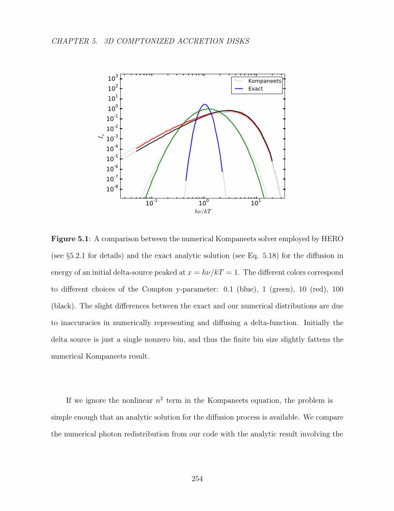
CHAPTER 5. 3D COMPTONIZED ACCRETION DISKS
10-1 100 101
hν/kT
10-810-710-610-510-410-310-210-1100101102103
I ν
KompaneetsExact
Figure 5.1: A comparison between the numerical Kompaneets solver employed by HERO
(see §5.2.1 for details) and the exact analytic solution (see Eq. 5.18) for the diffusion in
energy of an initial delta-source peaked at x = hν/kT = 1. The different colors correspond
to different choices of the Compton y-parameter: 0.1 (blue), 1 (green), 10 (red), 100
(black). The slight differences between the exact and our numerical distributions are due
to inaccuracies in numerically representing and diffusing a delta-function. Initially the
delta source is just a single nonzero bin, and thus the finite bin size slightly fattens the
numerical Kompaneets result.
If we ignore the nonlinear n2 term in the Kompaneets equation, the problem is
simple enough that an analytic solution for the diffusion process is available. We compare
the numerical photon redistribution from our code with the analytic result involving the
254
CHAPTER 5. 3D COMPTONIZED ACCRETION DISKS
complex integrals of Whittaker functions Wk,m(x) as worked out by Becker (2003), i.e.
fG(x, y) =32
πe−9y/4x−2
0 x−2e(x0−x)/2
∞∫0
e−u2y u sinh(πu)
(1 + 4u2)(9 + 4u2)W2,iu(x0)W2,iu(x)du
+e−x
2+e−x−2y
2
(2− x)(2− x0)
x0x, (5.18)
where x = hν/kT is the dimensionless frequency for the problem, fG(x) represents
the Green’s function spectral response of the system to a delta source injected at
frequency x0 after having evolved over a timescale corresponding to a given Compton
y = (4kT/mc2)nscat parameter. To compare with our numerical code, we set up the
diffusion problem such that x0 = 1 (i.e. we initialize HEROIC with a delta function
photon distribution peaked at x = 1), and we evolve the radiation field according to the
scheme as described in §5.2.1. In general, we find excellent agreement between HEROIC
and the analytic solution, with the biggest discrepancies occurring when there are a
moderate number of scatterings (i.e. when the Compton y-parameter is 0.1− 1).
These minor discrepancies are primarily induced by inaccuracies in numerically
representing and diffusing a delta-function. Initially the delta source is just a single
nonzero bin, and thus the finite bin size slightly fattens the numerical Kompaneets result.
Figure 5.2 shows the effect of frequency bin size on the limiting photon distribution
slopes. Having insufficient frequency resolutions results in more numerical diffusion,
which causes extra broadening of the photon distribution (compare widths of the dotted,
dashed, and solid curves in Fig 5.2).
255

CHAPTER 5. 3D COMPTONIZED ACCRETION DISKS
10-3 10-2 10-1 100 101 102 103
x=hν/kTgas
10-14
10-12
10-10
10-8
10-6
10-4
10-2
100
Fν
y=0.1
y=1
y=10
Figure 5.2: Here we compare the numerical result from our Kompaneets solver under
various frequency resolutions. The dotted, dashed, and solid lines correspond to 10,40,160
bins per frequency decade respectively. The thick solid line denotes the analytical solution
as computed from Eq. 5.18.
5.3.2 Escape Time Distributions
We would like to examine and benchmark HEROIC with the more difficult problem
of photon diffusion and Comptonization within a scattering atmosphere. The simplest
setup is that of a plane parallel atmosphere. Our goal is to compute the spectrum of
photons that escape from the upper/lower surface of the atmosphere, given that there is
a constant flux of photons injected at the midplane.
Since we have a robust numerical Kompaneets solver that calculates the spectrum
256
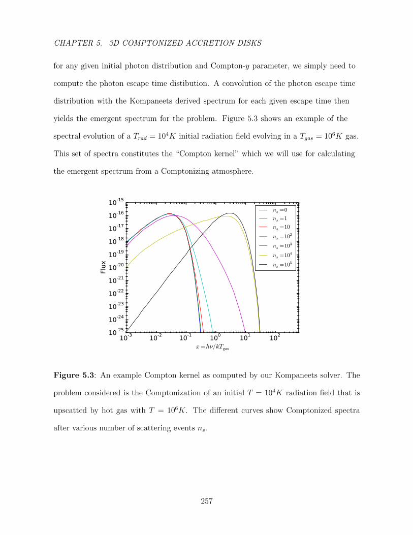
CHAPTER 5. 3D COMPTONIZED ACCRETION DISKS
for any given initial photon distribution and Compton-y parameter, we simply need to
compute the photon escape time distibution. A convolution of the photon escape time
distribution with the Kompaneets derived spectrum for each given escape time then
yields the emergent spectrum for the problem. Figure 5.3 shows an example of the
spectral evolution of a Trad = 104K initial radiation field evolving in a Tgas = 106K gas.
This set of spectra constitutes the “Compton kernel” which we will use for calculating
the emergent spectrum from a Comptonizing atmosphere.
10-3 10-2 10-1 100 101 102
x=hν/kTgas
10-25
10-24
10-23
10-22
10-21
10-20
10-19
10-18
10-17
10-16
10-15
Flux
ns =0
ns =1
ns =10
ns =102
ns =103
ns =104
ns =105
Figure 5.3: An example Compton kernel as computed by our Kompaneets solver. The
problem considered is the Comptonization of an initial T = 104K radiation field that is
upscatted by hot gas with T = 106K. The different curves show Comptonized spectra
after various number of scattering events ns.
257
CHAPTER 5. 3D COMPTONIZED ACCRETION DISKS
Plane Parallel Scattering Atmosphere
To get the escape time distribution for a 1D plane-parallel atmosphere, we simply solve
the diffusion equation, i.e.
dn
dt= D
d2n
dx2, (5.19)
where D = 1/3 is the diffusion constant corresponding to a three-dimensional diffusion
process2 in a homogeneous medium, x is the distance as measured in units of the
scattering mean free path, and t is measured in units of the number of scattering times.
The problem we seek to model is the process of photon diffusion from a midplane
injection point to an outer boundary surface. Specifically, we wish to determine the
probability distribution of the photon escape times. This quantity can be measured from
the diffusion equation as the escaping photon number flux at the surface. Instead of
taking the approach of Sunyaev & Titarchuk (1980) who tackle the problem analytically
via series expansions, we opt for a numerical solution.
We employ the same tri-diagonal implicit diffusion approach as we used previously
for numerically solving the Kompaneets problem. We only consider the upper half
portion of the slab, and make use of the symmetry of the problem through a reflecting
boundary condition at the midplane. The system is seeded with a spatial delta function
photon source at the midplane and we solve for the time/space evolution of photons.
The surface boundary is handled by setting purely outgoing radiation flux, which we
take from the two-stream framework of the radiative transfer equation:
dJ
dτ
∣∣∣∣surf
+√
3 J |surf = 0. (5.20)
2The coefficient 1/3 is also compatible with the two-stream approximation for radiative transfer
258
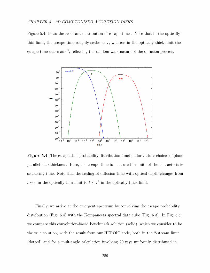
CHAPTER 5. 3D COMPTONIZED ACCRETION DISKS
Figure 5.4 shows the resultant distribution of escape times. Note that in the optically
thin limit, the escape time roughly scales as τ , whereas in the optically thick limit the
escape time scales as τ 2, reflecting the random walk nature of the diffusion process.
Figure 5.4: The escape time probability distribution function for various choices of plane
parallel slab thickness. Here, the escape time is measured in units of the characteristic
scattering time. Note that the scaling of diffusion time with optical depth changes from
t ∼ τ in the optically thin limit to t ∼ τ 2 in the optically thick limit.
Finally, we arrive at the emergent spectrum by convolving the escape probability
distribution (Fig. 5.4) with the Kompaneets spectral data cube (Fig. 5.3). In Fig. 5.5
we compare this convolution-based benchmark solution (solid), which we consider to be
the true solution, with the result from our HEROIC code, both in the 2-stream limit
(dotted) and for a multiangle calculation involving 20 rays uniformly distributed in
259
CHAPTER 5. 3D COMPTONIZED ACCRETION DISKS
cosine (dashed). The agreement is quite good (deviations at the 10% level), with the
largest errors arising at moderate optical depths (nscat ∼ 30).
For the above problem, we set up HEROIC with a purely scattering plane-parallel
atmosphere with 100 vertical depth points spaced equidistant in logarithm, with
τmin = 10−3. The code was run with a frequency resolution of 20 points per decade.
The midplane was treated as a reflecting boundary with an additional steady source
of blackbody radiation with effective temperature 104K3 coupled with a reflecting
boundary. At the upper surface of the atmosphere, the boundary condition was that
there is no incident radiation flux.
3The spectral shape for the injected flux is determined by the Planck function for T = 104K
260
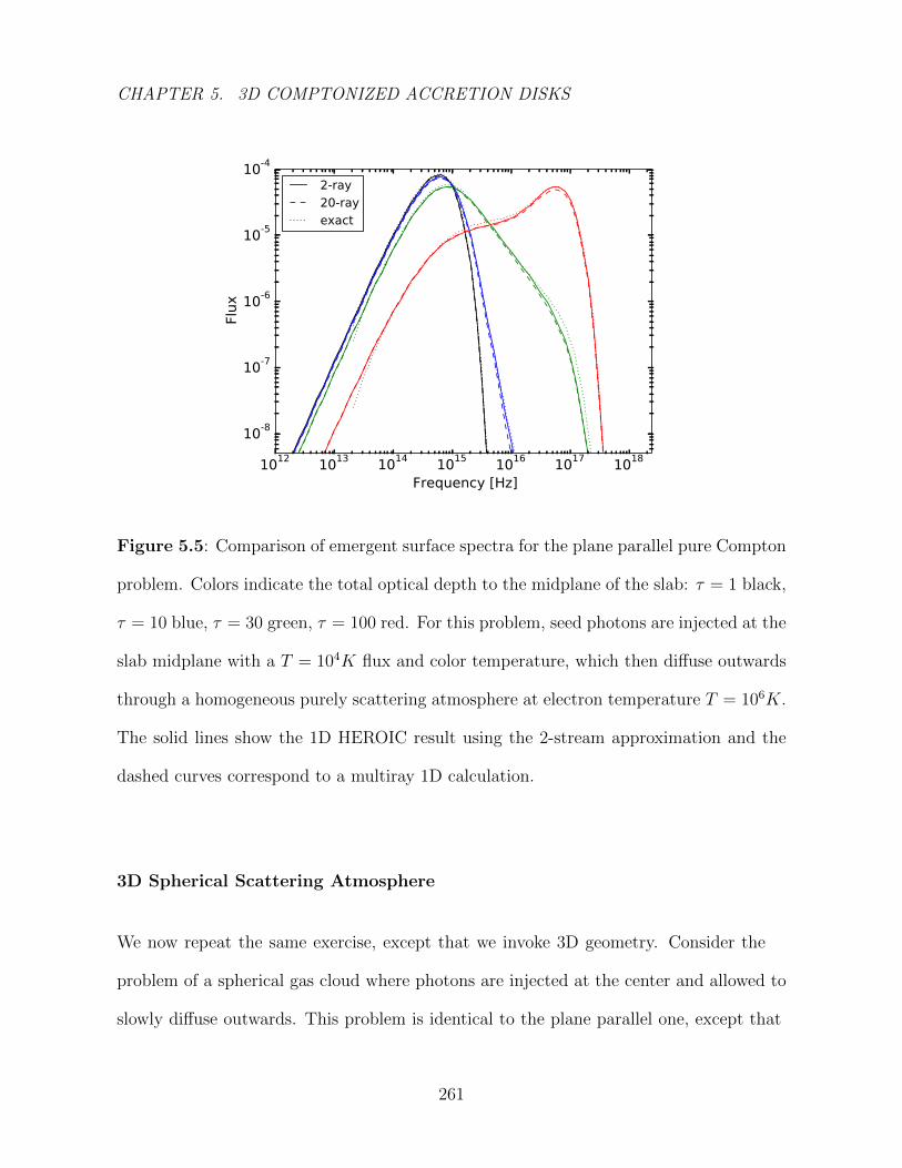
CHAPTER 5. 3D COMPTONIZED ACCRETION DISKS
1012 1013 1014 1015 1016 1017 1018
Frequency [Hz]
10-8
10-7
10-6
10-5
10-4
Flux
2-ray20-rayexact
Figure 5.5: Comparison of emergent surface spectra for the plane parallel pure Compton
problem. Colors indicate the total optical depth to the midplane of the slab: τ = 1 black,
τ = 10 blue, τ = 30 green, τ = 100 red. For this problem, seed photons are injected at the
slab midplane with a T = 104K flux and color temperature, which then diffuse outwards
through a homogeneous purely scattering atmosphere at electron temperature T = 106K.
The solid lines show the 1D HEROIC result using the 2-stream approximation and the
dashed curves correspond to a multiray 1D calculation.
3D Spherical Scattering Atmosphere
We now repeat the same exercise, except that we invoke 3D geometry. Consider the
problem of a spherical gas cloud where photons are injected at the center and allowed to
slowly diffuse outwards. This problem is identical to the plane parallel one, except that
261
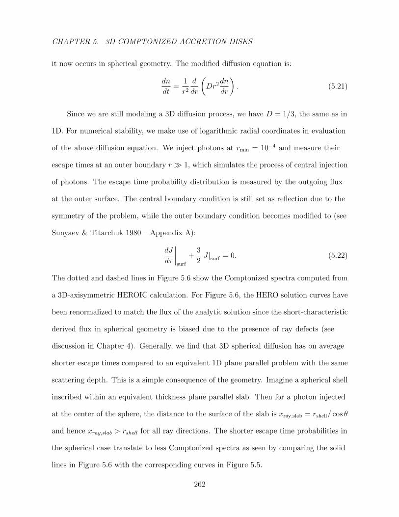
CHAPTER 5. 3D COMPTONIZED ACCRETION DISKS
it now occurs in spherical geometry. The modified diffusion equation is:
dn
dt=
1
r2
d
dr
(Dr2dn
dr
). (5.21)
Since we are still modeling a 3D diffusion process, we have D = 1/3, the same as in
1D. For numerical stability, we make use of logarithmic radial coordinates in evaluation
of the above diffusion equation. We inject photons at rmin = 10−4 and measure their
escape times at an outer boundary r 1, which simulates the process of central injection
of photons. The escape time probability distribution is measured by the outgoing flux
at the outer surface. The central boundary condition is still set as reflection due to the
symmetry of the problem, while the outer boundary condition becomes modified to (see
Sunyaev & Titarchuk 1980 – Appendix A):
dJ
dτ
∣∣∣∣surf
+3
2J |surf = 0. (5.22)
The dotted and dashed lines in Figure 5.6 show the Comptonized spectra computed from
a 3D-axisymmetric HEROIC calculation. For Figure 5.6, the HERO solution curves have
been renormalized to match the flux of the analytic solution since the short-characteristic
derived flux in spherical geometry is biased due to the presence of ray defects (see
discussion in Chapter 4). Generally, we find that 3D spherical diffusion has on average
shorter escape times compared to an equivalent 1D plane parallel problem with the same
scattering depth. This is a simple consequence of the geometry. Imagine a spherical shell
inscribed within an equivalent thickness plane parallel slab. Then for a photon injected
at the center of the sphere, the distance to the surface of the slab is xray,slab = rshell/ cos θ
and hence xray,slab > rshell for all ray directions. The shorter escape time probabilities in
the spherical case translate to less Comptonized spectra as seen by comparing the solid
lines in Figure 5.6 with the corresponding curves in Figure 5.5.
262
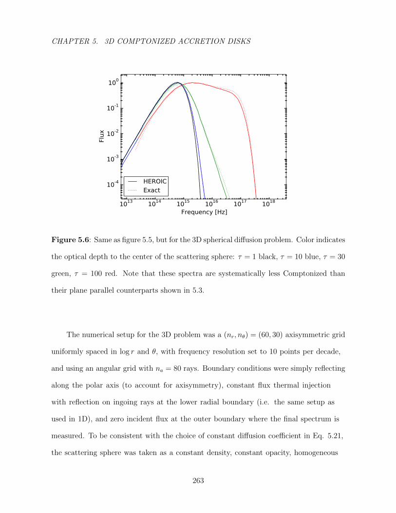
CHAPTER 5. 3D COMPTONIZED ACCRETION DISKS
1013 1014 1015 1016 1017 1018
Frequency [Hz]
10-4
10-3
10-2
10-1
100
Flux
HEROICExact
Figure 5.6: Same as figure 5.5, but for the 3D spherical diffusion problem. Color indicates
the optical depth to the center of the scattering sphere: τ = 1 black, τ = 10 blue, τ = 30
green, τ = 100 red. Note that these spectra are systematically less Comptonized than
their plane parallel counterparts shown in 5.3.
The numerical setup for the 3D problem was a (nr, nθ) = (60, 30) axisymmetric grid
uniformly spaced in log r and θ, with frequency resolution set to 10 points per decade,
and using an angular grid with na = 80 rays. Boundary conditions were simply reflecting
along the polar axis (to account for axisymmetry), constant flux thermal injection
with reflection on ingoing rays at the lower radial boundary (i.e. the same setup as
used in 1D), and zero incident flux at the outer boundary where the final spectrum is
measured. To be consistent with the choice of constant diffusion coefficient in Eq. 5.21,
the scattering sphere was taken as a constant density, constant opacity, homogeneous
263
CHAPTER 5. 3D COMPTONIZED ACCRETION DISKS
object.
5.4 Application – Accretion Disk
Most of the information that we have for black holes comes from observations of their
surrounding accretion disks. Through modelling the X-ray continuum of black hole
binary sources, it is possible to deduce the structure of the accretion disk, which can then
serve as an indirect probe of the physical properties of the black hole. Unfortunately, this
spectral modeling task is complicated by the fact that the accretion disk is scattering
dominated and hot. Scattering and Comptonization in the disk interior causes the
emerging radiation from the surface of the disk to have a “diluted” blackbody spectrum
with a color temperature given by
Tcol = fTeff , (5.23)
where f is the color correction factor and Teff is the effective temperature related to the
local disk flux. A key issue then is the determination of f since it determines the shape
of the resultant disk spectrum.
The earliest models typically assumed constant color correction factors f ∼ 1.5
(Mitsuda et al. 1984; Zhang et al. 1997a,b). More recently, much effort has gone towards
pinning down f in the case of X-ray binaries (Shimura & Takahara 1995; Merloni et al.
2000; Davis & Hubeny 2006) via sophisticated radiative transfer calculations. However
all prior work on determining f relied upon simplified 1D treatments of the problem.
Here, we present the first attempt at a 3D solution of the Compton disk problem that
self-consistently accounts for all relativistic and returning-radiation effects.
264
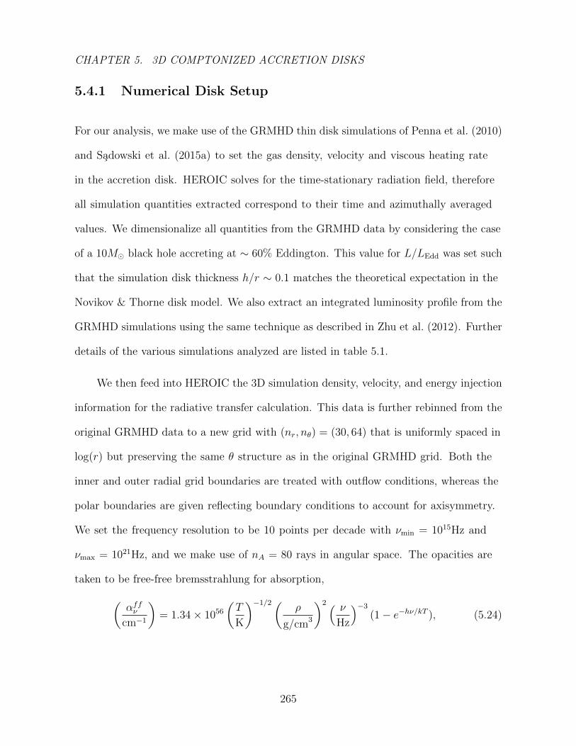
CHAPTER 5. 3D COMPTONIZED ACCRETION DISKS
5.4.1 Numerical Disk Setup
For our analysis, we make use of the GRMHD thin disk simulations of Penna et al. (2010)
and Sadowski et al. (2015a) to set the gas density, velocity and viscous heating rate
in the accretion disk. HEROIC solves for the time-stationary radiation field, therefore
all simulation quantities extracted correspond to their time and azimuthally averaged
values. We dimensionalize all quantities from the GRMHD data by considering the case
of a 10M black hole accreting at ∼ 60% Eddington. This value for L/LEdd was set such
that the simulation disk thickness h/r ∼ 0.1 matches the theoretical expectation in the
Novikov & Thorne disk model. We also extract an integrated luminosity profile from the
GRMHD simulations using the same technique as described in Zhu et al. (2012). Further
details of the various simulations analyzed are listed in table 5.1.
We then feed into HEROIC the 3D simulation density, velocity, and energy injection
information for the radiative transfer calculation. This data is further rebinned from the
original GRMHD data to a new grid with (nr, nθ) = (30, 64) that is uniformly spaced in
log(r) but preserving the same θ structure as in the original GRMHD grid. Both the
inner and outer radial grid boundaries are treated with outflow conditions, whereas the
polar boundaries are given reflecting boundary conditions to account for axisymmetry.
We set the frequency resolution to be 10 points per decade with νmin = 1015Hz and
νmax = 1021Hz, and we make use of nA = 80 rays in angular space. The opacities are
taken to be free-free bremsstrahlung for absorption,(αffν
cm−1
)= 1.34× 1056
(T
K
)−1/2(ρ
g/cm3
)2 ( ν
Hz
)−3
(1− e−hν/kT ), (5.24)
265
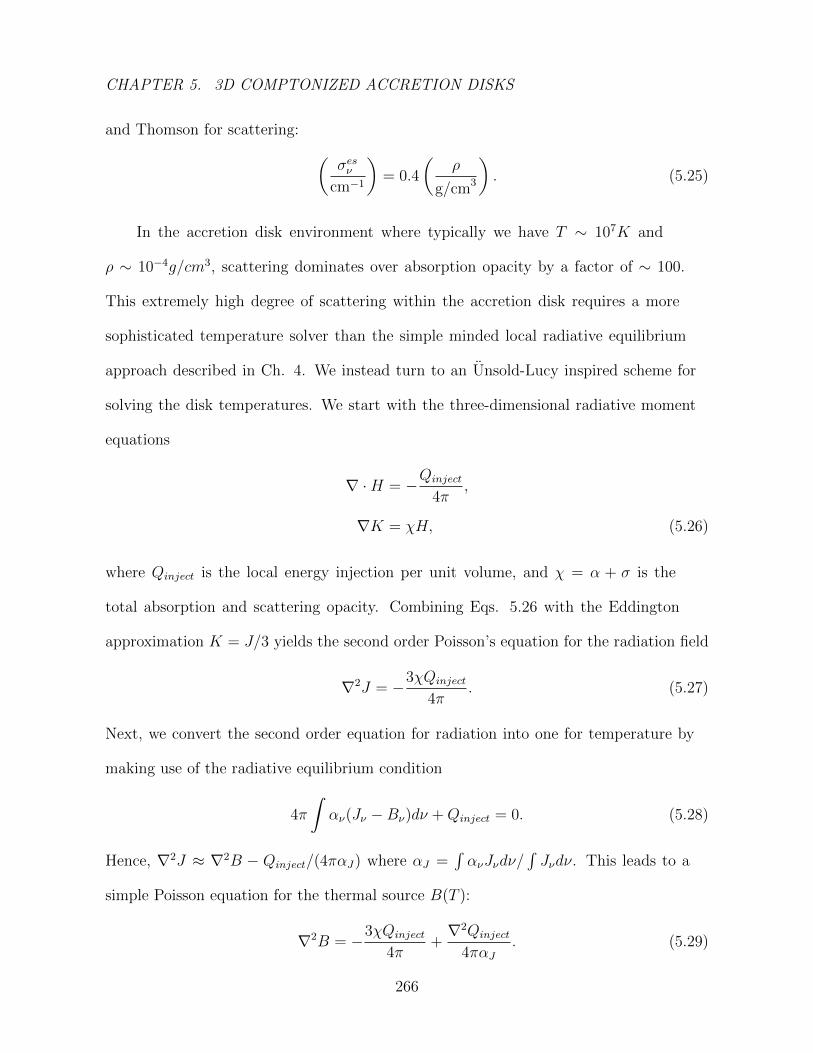
CHAPTER 5. 3D COMPTONIZED ACCRETION DISKS
and Thomson for scattering: (σesν
cm−1
)= 0.4
(ρ
g/cm3
). (5.25)
In the accretion disk environment where typically we have T ∼ 107K and
ρ ∼ 10−4g/cm3, scattering dominates over absorption opacity by a factor of ∼ 100.
This extremely high degree of scattering within the accretion disk requires a more
sophisticated temperature solver than the simple minded local radiative equilibrium
approach described in Ch. 4. We instead turn to an Unsold-Lucy inspired scheme for
solving the disk temperatures. We start with the three-dimensional radiative moment
equations
∇ ·H = −Qinject
4π,
∇K = χH, (5.26)
where Qinject is the local energy injection per unit volume, and χ = α + σ is the
total absorption and scattering opacity. Combining Eqs. 5.26 with the Eddington
approximation K = J/3 yields the second order Poisson’s equation for the radiation field
∇2J = −3χQinject
4π. (5.27)
Next, we convert the second order equation for radiation into one for temperature by
making use of the radiative equilibrium condition
4π
∫αν(Jν −Bν)dν +Qinject = 0. (5.28)
Hence, ∇2J ≈ ∇2B − Qinject/(4παJ) where αJ =∫ανJνdν/
∫Jνdν. This leads to a
simple Poisson equation for the thermal source B(T ):
∇2B = −3χQinject
4π+∇2Qinject
4παJ. (5.29)
266
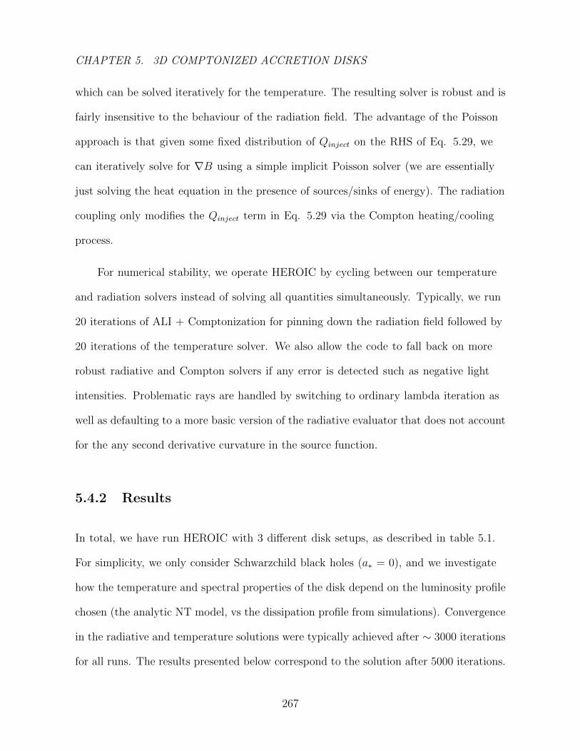
CHAPTER 5. 3D COMPTONIZED ACCRETION DISKS
which can be solved iteratively for the temperature. The resulting solver is robust and is
fairly insensitive to the behaviour of the radiation field. The advantage of the Poisson
approach is that given some fixed distribution of Qinject on the RHS of Eq. 5.29, we
can iteratively solve for ∇B using a simple implicit Poisson solver (we are essentially
just solving the heat equation in the presence of sources/sinks of energy). The radiation
coupling only modifies the Qinject term in Eq. 5.29 via the Compton heating/cooling
process.
For numerical stability, we operate HEROIC by cycling between our temperature
and radiation solvers instead of solving all quantities simultaneously. Typically, we run
20 iterations of ALI + Comptonization for pinning down the radiation field followed by
20 iterations of the temperature solver. We also allow the code to fall back on more
robust radiative and Compton solvers if any error is detected such as negative light
intensities. Problematic rays are handled by switching to ordinary lambda iteration as
well as defaulting to a more basic version of the radiative evaluator that does not account
for the any second derivative curvature in the source function.
5.4.2 Results
In total, we have run HEROIC with 3 different disk setups, as described in table 5.1.
For simplicity, we only consider Schwarzchild black holes (a∗ = 0), and we investigate
how the temperature and spectral properties of the disk depend on the luminosity profile
chosen (the analytic NT model, vs the dissipation profile from simulations). Convergence
in the radiative and temperature solutions were typically achieved after ∼ 3000 iterations
for all runs. The results presented below correspond to the solution after 5000 iterations.
267

CHAPTER 5. 3D COMPTONIZED ACCRETION DISKS
Table 5.1:: HEROIC disk parameters
Model Luminosity L/LEdd Energy Injection† Basis of Model‡
A 0.7 ρ3 NT
B 0.7 ρ3 GRMHD
C 0.6 sim GRMHD+Rad
† The prescription used to translate the total luminosity into a
3D energy injection distribution. For models A and B, we adopt
a centrally concentrated injection distribution that loads the en-
ergy according to ρ3 in each annulus. Model C simply takes the
radiation-gas net heating rate directly measured from the simu-
lation.
‡ NT – Novikov Thorne analytic energy injection profile; GRMHD
– based on numerical disk simulations of Penna et al. (2010);
GRMHD+Rad – based on numerical thin disk simulations of
Sadowski et al. (2015a)
Figure 5.7 shows the temperature distributions in the poloidal plane for the three
runs. We find in all cases that a hot optically-thin spherical corona forms around the
disk, and that the corona is hottest close to the black hole. In model B, we also find that
the final equilibrium temperature of the corona depends sensitively on the amount of
268

CHAPTER 5. 3D COMPTONIZED ACCRETION DISKS
energy injection present in the corona4. The base GRMHD disk model(Penna et al. 2010)
lacks any treatment of radiation, and so the derived temperature for the optically thin
coronal region is likely incorrect since it depends sensitively on gas heating distribution.
The temperatures of Model C on the other hand come directly from another GRMHD
code that includes a simplified treatment of radiation (Sadowski et al. 2015a). The
extreme temperatures seen along the polar axes of model C are a consequence of strong
radiative jets that are present in this disk simulation.
In Figure 5.8, we compare the disk temperature profile as computed by HEROIC
with the 1D radiative transfer calculation of TLUSTY.5 In both cases, the temperature
profile within the optically thick disk takes on a characteristic T ∝ τ 1/4 form, where τ
is the optical depth from the disk surface. The primary difference between TLUSTY
and HEROIC occurs above the disk’s scattering effective photosphere – the temperature
profile in HEROIC tends towards isothermality at all locations near the surface. This
is partly due to the 3D propagation of radiation, specifically the effect of returning
radiation from the disk. This incoming flux can penetrate downwards through the cool
photospheric surface to isothermalize via Compton heating of the local gas to match the
temperature of the incoming radiation.
Some differences between the 3D GRMHD result and the 1D TLUSTY calculation
are also due to differences in the mass distribution within the disk. TLUSTY recomputes
4In model B, we find that the coronal temperatures can vary by up to factors of 3, depending on the
exact energy injection prescription used (e.g. whether Qinj ∝ ρ or Qinj ∝ ρ3)
5Note: TLUSTY and HEROIC have slightly different setups for the vertical structure of energy
injection – TLUSTY injects energy within the vertical column according to a ρ1 prescription, whereas in
our computations with HEROIC, we used ρ3.
269
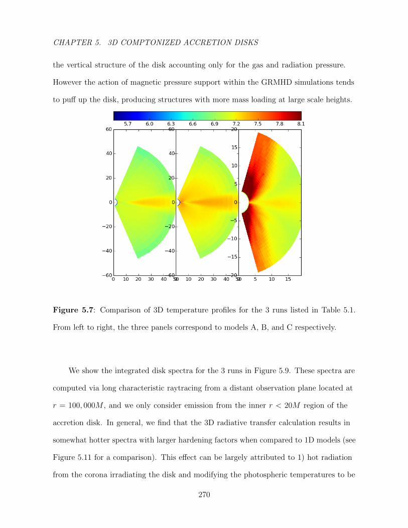
CHAPTER 5. 3D COMPTONIZED ACCRETION DISKS
the vertical structure of the disk accounting only for the gas and radiation pressure.
However the action of magnetic pressure support within the GRMHD simulations tends
to puff up the disk, producing structures with more mass loading at large scale heights.
Figure 5.7: Comparison of 3D temperature profiles for the 3 runs listed in Table 5.1.
From left to right, the three panels correspond to models A, B, and C respectively.
We show the integrated disk spectra for the 3 runs in Figure 5.9. These spectra are
computed via long characteristic raytracing from a distant observation plane located at
r = 100, 000M , and we only consider emission from the inner r < 20M region of the
accretion disk. In general, we find that the 3D radiative transfer calculation results in
somewhat hotter spectra with larger hardening factors when compared to 1D models (see
Figure 5.11 for a comparison). This effect can be largely attributed to 1) hot radiation
from the corona irradiating the disk and modifying the photospheric temperatures to be
270
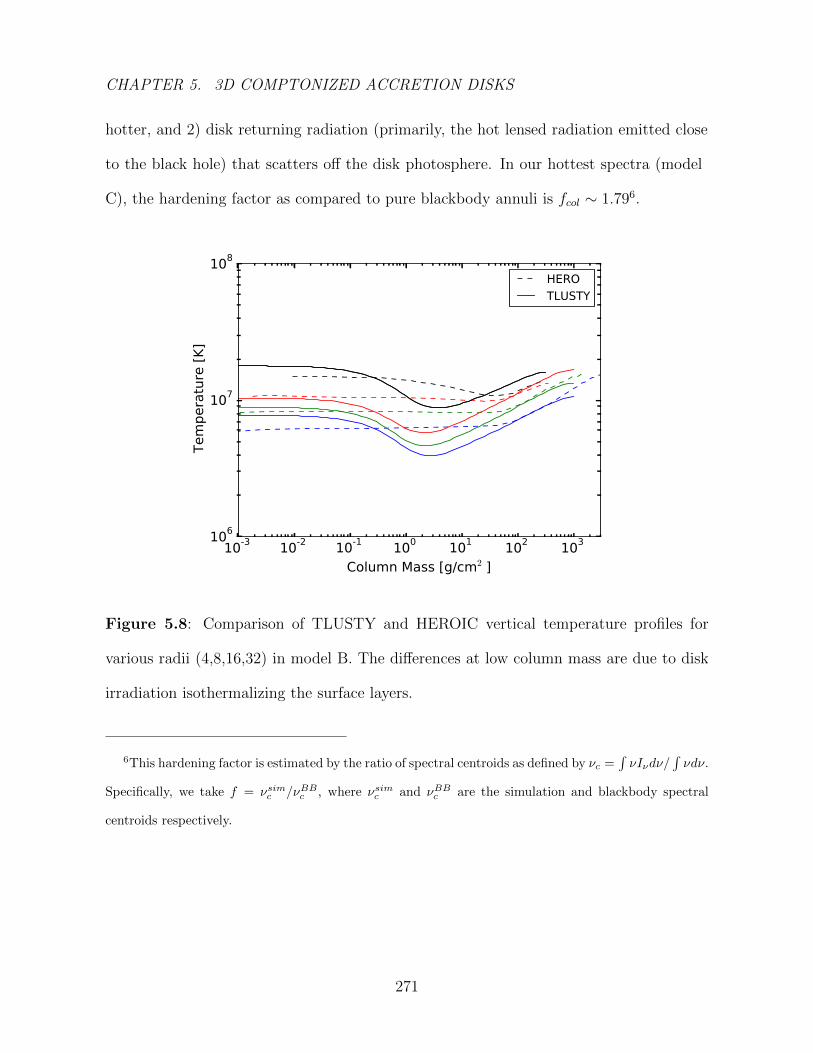
CHAPTER 5. 3D COMPTONIZED ACCRETION DISKS
hotter, and 2) disk returning radiation (primarily, the hot lensed radiation emitted close
to the black hole) that scatters off the disk photosphere. In our hottest spectra (model
C), the hardening factor as compared to pure blackbody annuli is fcol ∼ 1.796.
10-3 10-2 10-1 100 101 102 103
Column Mass [g/cm2 ]
106
107
108
Tem
pera
ture
[K]
HEROTLUSTY
Figure 5.8: Comparison of TLUSTY and HEROIC vertical temperature profiles for
various radii (4,8,16,32) in model B. The differences at low column mass are due to disk
irradiation isothermalizing the surface layers.
6This hardening factor is estimated by the ratio of spectral centroids as defined by νc =∫νIνdν/
∫νdν.
Specifically, we take f = νsimc /νBBc , where νsimc and νBBc are the simulation and blackbody spectral
centroids respectively.
271

CHAPTER 5. 3D COMPTONIZED ACCRETION DISKS
1017 1018 1019
Frequency [Hz]
10-7
10-6
10-5
10-4
10-3
10-2
10-1
100
Flux
a ∗=0, i=0o
BlackbodyNTGRMHD (2012)GRRMHD (2015)
1017 1018 1019
Frequency [Hz]
10-6
10-5
10-4
10-3
10-2
10-1
100
Flux
a ∗=0, i=60o
BlackbodyNTGRMHD (2012)GRRMHD (2015)
Figure 5.9: Comparison of integrated disk spectra for the inner disk (r < 20) as com-
puted by HEROIC for the three accretion disk models. The top panel shows spectra
for a the face-on observer (i = 0), whereas the right panel shows spectra for an inclined
(i = 60o) observer.
272
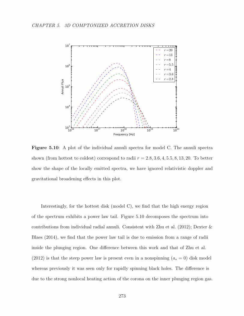
CHAPTER 5. 3D COMPTONIZED ACCRETION DISKS
1016 1017 1018 1019 1020
Frequency [Hz]
103
104
105
106
107
Annu
li Fl
ux
r=20
r=13
r=8
r=5.5
r=4
r=3.6
r=2.8
Figure 5.10: A plot of the individual annuli spectra for model C. The annuli spectra
shown (from hottest to coldest) correspond to radii r = 2.8, 3.6, 4, 5.5, 8, 13, 20. To better
show the shape of the locally emitted spectra, we have ignored relativistic doppler and
gravitational broadening effects in this plot.
Interestingly, for the hottest disk (model C), we find that the high energy region
of the spectrum exhibits a power law tail. Figure 5.10 decomposes the spectrum into
contributions from individual radial annuli. Consistent with Zhu et al. (2012); Dexter &
Blaes (2014), we find that the power law tail is due to emission from a range of radii
inside the plunging region. One difference between this work and that of Zhu et al.
(2012) is that the steep power law is present even in a nonspinning (a∗ = 0) disk model
whereas previously it was seen only for rapidly spinning black holes. The difference is
due to the strong nonlocal heating action of the corona on the inner plunging region gas.
273

CHAPTER 5. 3D COMPTONIZED ACCRETION DISKS
At high luminosities, radiation-dominated disks are expected to become effectively
optically thin. When coupled to the fact that the inner radii still produce a significant
amount of emission (e.g. Noble et al. 2009), we find that this leads to a rapid increase in
gas temperature in the inner radii resulting in a high-energy powerlaw spectral tail from
the superposition of nearly saturated Wien spectra.
We note that this thermal superposition mechanism for producing high energy
power-laws is different from another earlier idea known as bulk Comptonization
(Blandford & Payne 1981; Titarchuk, Mastichiadis & Kylafis 1997; Titarchuk & Zannias
1998), which also predicts the onset of power laws. For bulk Comptonization, relativistic
boosting from bulk gas motions within a converging flow can produce power law tails by
upscattering the incident disk light. The bulk Comptonization mechanism is extremely
sensitive to the nature of the irradiating thermal light(Psaltis & Lamb 1999), and also
has a strong viewing inclination dependence (Niedzwiecki 2005). In our calculations, we
do not find any change in the power law behaviour at different viewing inclinations (i.e.
compare how similar the power law slope and strengths are in Fig. 5.9 for two different
inclinations), so it is unlikely that the HEROIC power law region is sourced by bulk
Comptonization.
5.5 Discussion
Recently, there has been great interest in fitting X-ray spectral observations of black
holes for the purpose of measuring black hole spin (Zhang et al. 1997a; Shafee et al.
2006; Steiner et al. 2009a; McClintock et al. 2011). The ‘continuum fitting method’ relies
upon accurate modeling the soft X-ray thermal continuum emission. In particular, the
274
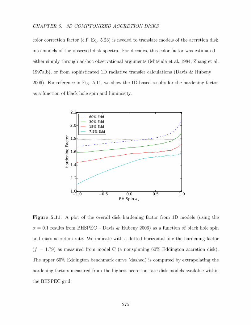
CHAPTER 5. 3D COMPTONIZED ACCRETION DISKS
color correction factor (c.f. Eq. 5.23) is needed to translate models of the accretion disk
into models of the observed disk spectra. For decades, this color factor was estimated
either simply through ad-hoc observational arguments (Mitsuda et al. 1984; Zhang et al.
1997a,b), or from sophisticated 1D radiative transfer calculations (Davis & Hubeny
2006). For reference in Fig. 5.11, we show the 1D-based results for the hardening factor
as a function of black hole spin and luminosity.
1.0 0.5 0.0 0.5 1.0BH Spin a ∗
1.0
1.2
1.4
1.6
1.8
2.0
2.2
Hard
enin
g Fa
ctor
60% Edd30% Edd15% Edd7.5% Edd
Figure 5.11: A plot of the overall disk hardening factor from 1D models (using the
α = 0.1 results from BHSPEC – Davis & Hubeny 2006) as a function of black hole spin
and mass accretion rate. We indicate with a dotted horizontal line the hardening factor
(f = 1.79) as measured from model C (a nonspinning 60% Eddington accretion disk).
The upper 60% Eddington benchmark curve (dashed) is computed by extrapolating the
hardening factors measured from the highest accretion rate disk models available within
the BHSPEC grid.
275

CHAPTER 5. 3D COMPTONIZED ACCRETION DISKS
The calculations in §5.4.2 of this work allow for perhaps the best estimation of
the hardening factor to date (i.e. a hardening factor based on numerical simulations
of black holes with 3D radiation transport). Our 3D result (Fig. 5.9) yields a slightly
higher overall hardening factor at f = 1.79 for a nonspinning black hole accreting at 60%
Eddington. We see in Figure 5.11 that this new calculation is not too different from the
previous 1D estimates.
Of particular interest is the impact that the new spectral hardening factor has on
the recovered spins of black hole systems. Unfortunately, due to the high accretion rates
of our simulated disks (L/LEdd ∼ 0.6), the disk spectrum is outside the parameter ranges
of the currently used X-ray disk models. Rather than directly fitting our simulated
spectrum with the current spectral models, we instead rely on the trend seen in Fig.
5.11 between the color correction factor and spin at a fixed L/LEdd. We observe a minor
discrepancy in ∆f ∼ 0.05 between 1D and 3D models, which when translated in terms
of a spin bias corresponds to measuring a∗ = 0.3 for a a∗ = 0 system. If the black hole
were highly rotating, then the same ∆f ∼ 0.05 would translate to a spin discrepancy of
(a∗ = 0.88) → (a∗ = 0.83). This estimate for the spin bias is also consistent with the
experiences of observers (Steiner 2015, private communication)7 when fitting disk models
using fixed spectral hardening factors.
As mentioned earlier, it is the disk returning radiation that causes the additional
hardening we see in 3D models. In figure 5.12, we compare both the emergent and
returning fluxes as a function of radius. Typically, our HEROIC calculation yields larger
7Steiner (2015, private communication) typically finds that ∆f ∼ 0.05 translates to spin biases at the
level of (a∗ = 0.1)→ (a∗ = 0) or (a∗ = 0.87)→ (a∗ = 0.83).
276
CHAPTER 5. 3D COMPTONIZED ACCRETION DISKS
returning fluxes compared to previous work with analytic disks (Cunningham 1976; Li
et al. 2005). For instance HEROIC predicts the returning flux to be at the ∼ 10% level,
whereas figure 2 of Li et al. (2005) suggests it is only at the few percent level.
Disk flaring was ignored in the work of Li et al. (2005) and is likely the cause for
HEROIC having such large returning radiation fluxes (see rightmost panel of Figure 5.7,
model C, for the most obvious example of flaring in our simulated disks). For a flared
disk, the additional flux scales as simply
F = ξLi
4πr2,(5.30)
where Li is the characteristic luminosity of the interior irradiating source (i.e. the hot
innermost annuli that shine on the rest), and ξ = rd(h/r)/dr is a geometric scaling
constant related to the flaring angle within the disk. If Li is large, then even tiny values
of ξ (i.e. small flaring angles) can still result in substantial irradiated flux at the flared
surface.
277
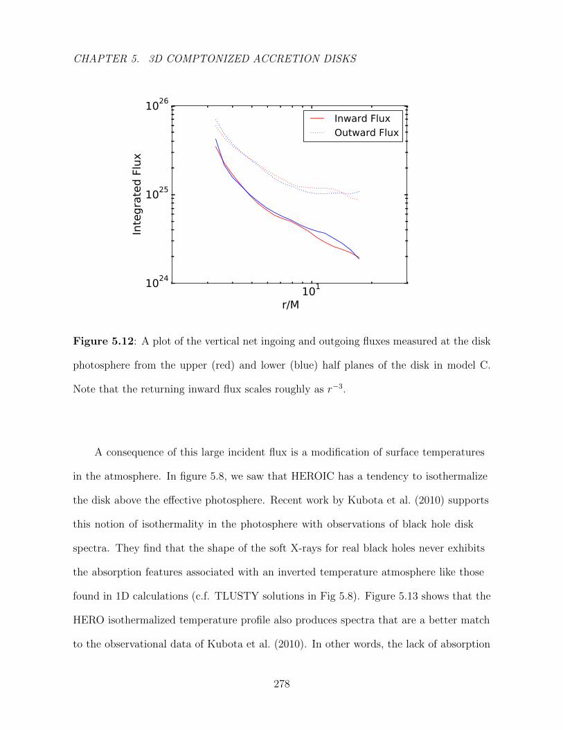
CHAPTER 5. 3D COMPTONIZED ACCRETION DISKS
101
r/M
1024
1025
1026
Inte
grat
ed F
lux
Inward FluxOutward Flux
Figure 5.12: A plot of the vertical net ingoing and outgoing fluxes measured at the disk
photosphere from the upper (red) and lower (blue) half planes of the disk in model C.
Note that the returning inward flux scales roughly as r−3.
A consequence of this large incident flux is a modification of surface temperatures
in the atmosphere. In figure 5.8, we saw that HEROIC has a tendency to isothermalize
the disk above the effective photosphere. Recent work by Kubota et al. (2010) supports
this notion of isothermality in the photosphere with observations of black hole disk
spectra. They find that the shape of the soft X-rays for real black holes never exhibits
the absorption features associated with an inverted temperature atmosphere like those
found in 1D calculations (c.f. TLUSTY solutions in Fig 5.8). Figure 5.13 shows that the
HERO isothermalized temperature profile also produces spectra that are a better match
to the observational data of Kubota et al. (2010). In other words, the lack of absorption
278
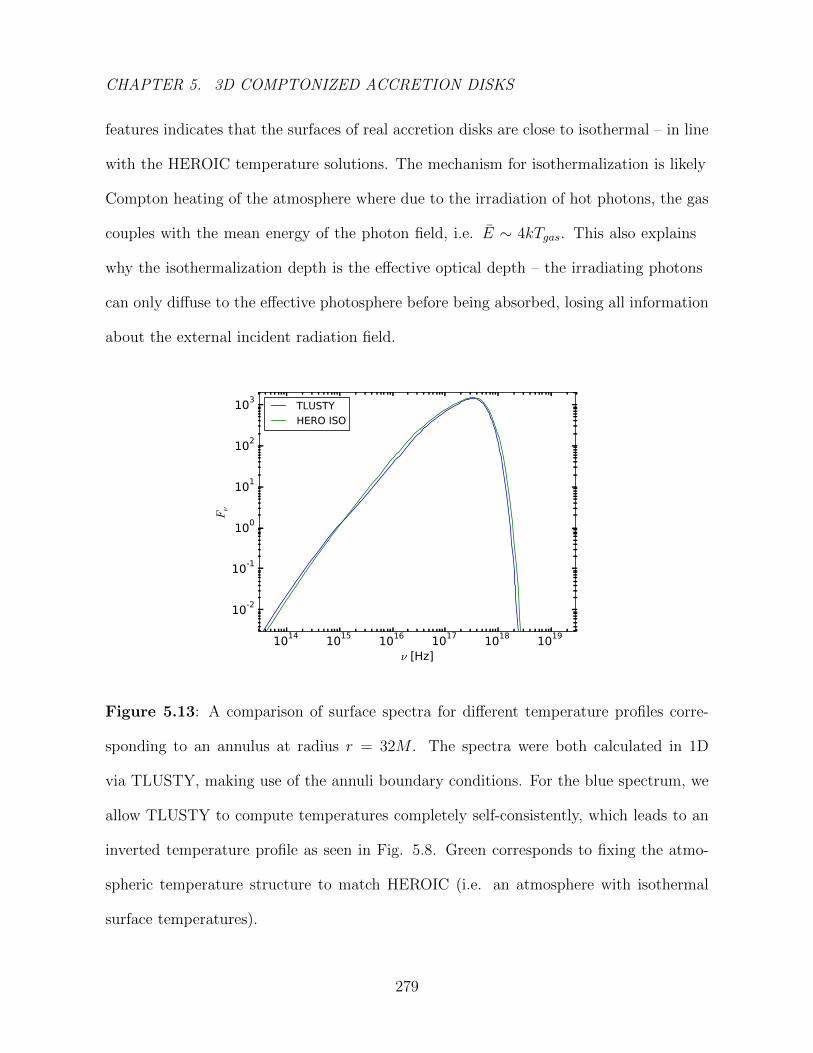
CHAPTER 5. 3D COMPTONIZED ACCRETION DISKS
features indicates that the surfaces of real accretion disks are close to isothermal – in line
with the HEROIC temperature solutions. The mechanism for isothermalization is likely
Compton heating of the atmosphere where due to the irradiation of hot photons, the gas
couples with the mean energy of the photon field, i.e. E ∼ 4kTgas. This also explains
why the isothermalization depth is the effective optical depth – the irradiating photons
can only diffuse to the effective photosphere before being absorbed, losing all information
about the external incident radiation field.
1014 1015 1016 1017 1018 1019
ν [Hz]
10-2
10-1
100
101
102
103
Fν
TLUSTYHERO ISO
Figure 5.13: A comparison of surface spectra for different temperature profiles corre-
sponding to an annulus at radius r = 32M . The spectra were both calculated in 1D
via TLUSTY, making use of the annuli boundary conditions. For the blue spectrum, we
allow TLUSTY to compute temperatures completely self-consistently, which leads to an
inverted temperature profile as seen in Fig. 5.8. Green corresponds to fixing the atmo-
spheric temperature structure to match HEROIC (i.e. an atmosphere with isothermal
surface temperatures).
279
CHAPTER 5. 3D COMPTONIZED ACCRETION DISKS
5.6 Summary
In this work, we develop a new 3D relativistic Comptonization module within the
framework of the radiative transfer code HERO. In this enhanced code HEROIC,
Comptonization is handled through a quadratic solver that evolves light rays by means
of a modified Comptonized source function. We test our Comptonization module by
comparing with exact solutions of light diffusing through purely scattering media. These
exact solutions are generated by consideration of the photon escape time probability
distribution. We find excellent agreement between HEROIC and the exact solutions for
both 1D and 3D test problems.
Next, we apply HEROIC to the astrophysical problem of radiation emerging from
an accretion disk. We calculate the self consistent temperature and radiation fields
throughout the accretion disk taking into account relativistic effects, returning disk
radiation, and Compton cooling. The complete solution results in a two-phase disk
structure, with a hot spherical corona surrounding a cooler thermal disk. Performing
raytracing on the solution yields integrated disk spectra with slightly higher spectral
hardening factors compared to previous 1D based estimates (i.e. we find f = 1.79 for our
hottest disk models, compared to f ∼ 1.75 in a 1D model).
We also verify the Zhu et al. (2012) result of a high-energy power law tail feature
emerging in the black hole accretion disk spectrum. We find the power law arises from
the superposition of saturated Wien spectra from the inner plunging region. Another
feature of the 3D radiation calculation is the impact of returning radiation – namely, we
find that the irradiation flux from the hot inner annuli tends to isothermalize the surface
layers of the disk, and is also responsible for the extra degree of spectral hardening
280
CHAPTER 5. 3D COMPTONIZED ACCRETION DISKS
present in our 3D models.
We stress that the results presented here are preliminary. In the future, we will
extend our analysis to the case of spinning black holes, as well as more exotic states of
black hole accretion such as the supereddington regime. A current limitation of HEROIC
is its inability to treat outflows and jets due to the lack of a proper advection operator
in its temperature solver. Relativistically hot systems are also presently inaccessable
to HEROIC due to the soft Comptonization assumption inherent with the Kompaneets
operator approach. Future releases of the code will include a switch to toggle between
Kompaneets and a new relativistic photon redistribution kernel to handle the case of
extremely hot Comptonization.
281
Chapter 6
Summary and Future Directions
6.1 Summary
In this thesis, we investigate the radiation from accretion disks around black holes.
A major motivating factor for studying radiation from accretion disks is the recent
observational effort to measure black hole spin via spectral fitting of the X-ray thermal
continuum. The task of continuum fitting is complicated by several factors: 1) the
high degree of scattering present within the accretion disk leads to complex nonlocal
coupling of the radiation field; 2) the true structure of the disk may deviate from the
standard model of Novikov & Thorne (1973); and 3) the presence of a hot comptonizing
corona can complicate the determination of the thermal disk component of the spectra.
To combat these issues, a firmer theoretical understanding of the underlying radiative
processes is needed.
This thesis tries to address some of the limitations lurking in the spectral modeling
282
CHAPTER 6. SUMMARY AND FUTURE DIRECTIONS
business. Our exploration starts in Chapter 2, where we compute the spectral signatures
of recent GRMHD global simulations of turbulent accretion. We calculate synthetic disk
spectra by combining 1D-radiative transfer calculations with relativistic raytracing. We
find that our numerical GRMHD turbulent accretion disks are nearly indistinguishable
from prevailing analytic disk models in their spectra. The only surprise from this exercise
was for the spinning black hole case. We observed a weak power law tail at high energies
that was being generated by the hot comptonized emission of the plunging region.
However due to the 1D treatment of problem becoming increasingly invalid inside the
plunging region, doubts were raised on the veracity of this apparent power law. This
motivated the need for 3D radiative transfer calculations to confirm the result hinted at
by the 1D calculation.
Chapter 3 builds upon the 1D disk modeling theme to answer a longstanding
question: how can radiatively dominated disks remain thermally stable? The prediction
from the standard disk model is that beyond moderate accretion rates (L > 0.05LEdd),
the disk should enter a radiation dominated regime that is susceptable to a runaway
heating/cooling process (the thermal instability). Yet there are many observations of
well-behaved accretion disks accreting at L ∼ 0.3LEdd that are stable for long periods
of time. Our 1D disk model reconciles this tension between theory and observations by
noting that the introduction of turbulent mixing leads to a suppression of the radiative
heat flux, which restores stability up to L ∼ 0.5LEdd.
We take a departure from the 1D radiative modelling approach starting in chapter
4. Here we develop HERO, a new 3D relativistic radiative transfer code. The bulk of this
chapter is simply devoted to explaining how HERO operates. We also present a series of
1D, 2D, 3D, and 4D(relativistic) benchmark tests to verify that the code is producing
283
CHAPTER 6. SUMMARY AND FUTURE DIRECTIONS
physically reasonable results.
Chapter 5 focuses on extending the capabilities of HERO by adding a Compton
module to the code. The new upgraded code is named HEROIC – HERO Including
Comptonization. Again, we benchmark HEROIC against a suite of 1D and 3D analytic
solutions before turning to the astrophysical application of a Comptonized thin accretion
disk. We find that our disk spectra from the 3D radiative calculations match fairly closely
to the earlier 1D estimates. The slight differences that arise are due to a combination
of: 1) returning radiation providing additional heating in the disk photosphere, and 2)
differences in the energy injection/mass profile for 1D vs 3D.
6.2 Future Directions
HEROIC represents a first attempt at a robust 3D general-relativistic radiative-transfer
code. It is designed to work for all manners of optically thick Compton problems with
Tgas < 108K (i.e. the nonrelativistic Comptonization regime). This covers a wide range
of problems, and several of these potential applications are listed below.
6.2.1 Astrophysical Applications
Perhaps the most immediately obvious application of HEROIC is revisiting the spin
fitting bias calculation of (Zhu et al. 2012). It would be useful to see how the 3D spectral
analysis differs from the 1D analysis to check if the GRMHD disk deviations for BH spin
fitting are still negligible. Based on the preliminary results of Chapter 5, it is likely that
the updated 3D HEROIC calculation would have larger deviations than was previously
284
CHAPTER 6. SUMMARY AND FUTURE DIRECTIONS
found in 1D.
Suppereddington accretion disks are another interesting application for HEROIC.
This relates to the spectral modeling of ultraluminous X-ray (ULX) sources, which have
luminosities that greatly exceed (by factors of up to 1000 – Farrell et al. 2009) the
Eddington limit for a typical stellar mass black hole (M ∼ 10M). This large violation
of the Eddington limit suggests that these objects probably correspond to intermediate
mass black holes with M 10M. An interesting project would be for someone to
calculate the spectral properties of numerically simulated ULXs via HEROIC. This
would test if there is truly an upper limit to the apparent luminosity as seen by distant
observers to help settle the debate on the existence of IMBHs.
Computing the radiation from BH jets would be another interesting future
application of HERO. Jet-structures, their formation, acceleration, and their relationship
to the accretion phenomena is still an area of open research(Tchekhovskoy et al. 2011;
Tchekhovskoy & McKinney 2012). Luckily, there is a wealth of observational data
available from a variety of astrophysical systems (e.g. AGN, microquasars). Due to the
importance of relativity and 3D effects on jet production, HERO would be an ideal code
to analyze the observable consequences of jets produced by numerical simulations.
6.2.2 Future Plans for HERO
HERO as a code is still in its infancy – so far, it has only been applied to the problem of
modeling thermal emission from BH accretion disks. Below we discuss a partial list of
features that we intend to explore in future releases.
Perhaps the feature with the most immediate astrophysical payoff would be the
285
CHAPTER 6. SUMMARY AND FUTURE DIRECTIONS
inclusion of line opacities and emissivities. A proof of concept has already been
demonstrated from investigations in chapter 4 (i.e. the iron line reflection problem),
which involved handling line emission for a single atomic transition. Iron line fitting
is an active area of research since it offers another way of measuring black hole spin.
Unfortunately, there are several major uncertainties underpinning the whole business
of fluorescence line modeling. For instance, the exact nature of the disk illumination
from a hot corona is not well understood. The hope is that HERO will be able to
self-consistently calculate both the coronal component and reflection components of the
radiation field. If successful, this exercise would be extremely useful for constraining
illumination models for the iron line profile.
Adding time dependence to HERO is another alluring next step. The variability
properties of black hole systems are very diverse and depend on the spectral state of
the BH. Particularly interesting is the phenomenon of high-frequency Quasi-Periodic
Oscillations. These QPOs are seen as narrow peaks in the power spectrum that sometime
arrive in packs with fixed integer frequency ratios. These are thought to be caused by
resonant coupling of epicyclic frequencies in the disc although there is still much debate
on their true origin. It would be interesting to see if the time dependent emission as
computed by HERO for a realistic accretion flow leads to the phenomenon of QPOs.
Other ideas related to time dependence includes the phenomenon of X-ray reverberation
in accretion disks. It would be very interesting to see if we can reproduce the same
time lags in a simulation as the lags observed in nature. So far, we have made some
minor progress towards developing a time-dependent HERO package in collaboration
with Olek Sadowski by interfacing with his hydrodynamic KORAL code via a Variable
Eddington Tensor approach. We have only completed a few preliminary test problems
286
CHAPTER 6. SUMMARY AND FUTURE DIRECTIONS
that demonstrate proof of concept (i.e. shadow tests, crossing beam tests, relativistic
light bending tests, etc...).
Polarization offers yet another dimension for gathering information about
astrophysical sources. One of the major goals of the Event Horizon Telescope
collaboration is the measure the linear polarization of our Galaxy’s radio emission at
10µas scales. A scintillating project would therefore be to add polarization capabilities to
HERO and calculate the expected polarized field from to a realistic simulated accretion
flow. The main advantage HERO has is that it correctly computes the self-consistent
scattered radiation field in all parts of the flow (including optically thick parts).
Other desirable features for HERO would be the ability to handle relativistic
Comptonization. This would require an overhaul of the current Compton solver
from the current Kompaneets diffusion approach to a more detailed frequency by
frequency redistribution analysis. Another future improvement would be the ability
to handle angle dependent scattering kernels instead of the isotropic approximation
that is currently in place. This becomes especially important in the limit of relativistic
scattering. For studying emission from say nonthermal shocks in jets, it would be nice
if the Comptonization module also had support for nonthermal electron temperature
distributions.
287
References
Abel, T., & Wandelt, B. D. 2002, MNRAS, 330, L53
Abramowicz M. A., Czerny B., Lasota J. P., Szuszkiewicz E., 1988, ApJ, 332, 646
Abramowicz M.A., Chen X., Kato S., Lasota J.-P., Regev O., 1995, ApJ, 438, 37
Abramowicz M. A., Lanza A., Percival M. J., 1997, ApJ, 479, 179
Abramowicz M. A., Fragile C. P., 2011, eprint, arXiv:1104.5499
Abramowicz M. A., Kluzniak W. 2001, A&A, 374:L19-20
Afshordi N., Paczynski B., 2003, ApJ, 592, 354
Agol E., Krolik J., Turner N. J., Stone J. M., 2001, ApJ, 558, 543
Anninos P., Fragile P.C., Salmonson J., 2005, ApJ, 635, 723
Arnaud, K. A. 1996, in Jacoby G. H., Barnes J., eds, Astronomical Society of
the Pacific Conference Series, Vol. 101, Astronomical Data Analysis Software and
Systems V, San Francisco: ASP, 17
Balbus S. A., Hawley J. F., 1991, ApJ, 376, 214
Balbus S.A., Hawley J.F., 1998, Rev. Mod. Phys., 70, 1
Bath G. T., Pringle J. E., 1982, MNRAS, 199, 267
Bardeen J.M., Press W.H., Teukolsky S.A., 1972, ApJ, 178, 347
Becker P.A., 2003, MNRAS, 343, 215
Beckwith K., Hawley J. F., Krolik J. H., 2008a MNRAS, 390, 21
Beckwith K., Hawley J. F., Krolik J. H., 2008b ApJ, 678, 1180
288

REFERENCES
Beckwith K., Stone J. M., 2011, ApJS, 193, 6
Bianchi S., 2008, A&A, 490, 461
Bisnovatyi-Kogan G. S., Blinnikov S. I., 1977, A&A, 59, 111
Bjorkman J. E., Wood K., 2001, ApJ, 554, 615
Blandford R. D., Payne, D. G., 1981, MNRAS, 194, 1033
Blandford R.D., Payne D.G., 1982, MNRAS, 199, 883
Blandford R.D., Znajek R.L., 1977, MNRAS, 179, 433
Blaes O.M., Davis S.W., Hirose S., Krolik J.H., Stone J.M., 2006, ApJ, 645, 1402
Blaes O., Krolik J. H., Hirose S., Shabaltas N., 2011, ApJ, 733, 110
Blandford R.D., Begelman M.C., 1999, MNRAS, 303, 1
Blandford R. D., Payne, D. G., 1982, MNRAS, 199, 883
Blandford R. D., Znajek R. L. 1977, MNRAS, 179, 433
Bohn A., Throwe W., Hebert F., Henriksson K., Bunandar D., Taylor N. W.,
Scheel M. A., 2014, preprint (arXiv:1410.7775)
Bolton C. T., 1972, Nat, 240, 124
Broderick A. E., Blandford R., 2003, MNRAS, 342, 1280
Broderick A.E., Loeb A., Narayan R., 2009, ApJ, 701, 1357
Broderick A.E., Narayan R., Kormendy J., Perlman E.S., Rieke M.J., Doeleman
S.S., 2015, arXiv:1503.03873
Bruenn S. W., Dirk C. J., Mezzacappa A., Hayes J. C., Blondin J. M., Hix W. R.,
Messer O. E. B., 2006, JPhCS, 46, 393
Brunner T.A., 2002, Sandia National Labs Report, doi:10.2172/800993
Burrows A., Young T., Pinto P., Eastman R., Thompson T. A., 2000, ApJ, 539,
865
Cannizzo J. K., 1992, ApJ, 385, 94
Cantrell A. G. et al., 2010, ApJ, 710, 1127
289

REFERENCES
Canuto, C., Hussaini, M.Y., Quarteroni, A., Zang, Th.A., 1988, Spectral Methods,
Springer-Verlag Berlin Heidelberg
Chakrabarti S., Cox T. J., Hernquist L., Hopkins P. F., Robertson B., Di Matteo
T., 2007, ApJ, 658, 840
Chandrasekhar S., 1950, Radiative Transfer, Oxford, Clarendon Press
Chandrasekhar S., 1967, in An Introduction to the Study of Stellar Structure,
University of Chicago Press, Chicago, pp.56-59
Chan C.-K., Psaltis D., & Ozel, F., 2013, ApJ, 777, 13
Chang J.S., Cooper G., 1970, J. Comp. Phys, 6, 1
Chung T.J., 2010, Computational Fluid Dynamics, University of Cambridge Press,
Cambridge, p.1010
Ciesielski A., Wielgus M., Kluzniak W., Sadowski A., Abramowicz M., Lasota
J.-P., Rebusco P., 2012, A&A, 538, 148
Commercon B., Teyssier R., Audit E., Hennebelle P., Chabrier G., 2011, A&A,
529A, 35
Contopoulos I., Kazanas D., 1998, ApJ, 508, 859
Coppi P.S., 1991, PhDT, 2
Cunningham C. T., Bardeen J. M., 1973, ApJ, 183, 237
Cunningham C., 1976, ApJ, 208, 534
Dauser T., Wilms J., Reynolds C.S., Brenneman L.W., 2010, MNRAS, 409, 1534
Dauser T., Garcia J., Wilms J., Bock M., Brenneman L.W., Falanga M., Fukumura
K., Reynolds C.S., 2013, MNRAS, 430, 1694
Davis S. W., Blaes O. M., Hubeny I., Turner N. J., 2005, ApJ, 621, 372
Davis S. W., Done C., Blaes O. M., 2006b, ApJ, 647, 525
Davis S. W., Blaes O. M., Hirose S., Krolik J. H., 2009, ApJ, 703, 569
Davis S. W., Stone J. M., Pessah M. E., 2010, ApJ, 713, 52
Davis S. W., Stone J. M., & Jiang Y.-F., 2012, ApJS, 199, 9
290
REFERENCES
Davis S. W., Hubeny I. 2006, ApJS, 164, 530
Del Zanna L., Zanotti O., Bucciantini N., Londrillo P., 2007, A&A, 473, 11
De Villiers J., Hawley J. F., Krolik J. H., 2003, ApJ, 599, 1238
De Villiers J.-P., Hawley J. F., 2003, ApJ, 589, 458
Dexter J., Agol E., 2009, ApJ, 696, 1616
Dexter J., Quataert E., 2012, MNRAS, submitted
Dexter J., Blaes O., 2014, MNRAS, 438, 3352
D’Inverno R., 1992, Introducing Einstein’s Relativity, Oxford-Clarendon Press
Doeleman S. et al., 2009, Astro2010: The Astronomy and Astrophysics Decadal
Survey, Science White Papers, No., 68
Dolence J. C., Gammie C. F., Moscibrodzka M., Leung P. K., 2009, ApJS, 184, 387
Done C., Wardzinski G., Gierlinski M., 2004, MNRAS, 349, 393
Dovciak M., Karas V., Yaqoob T., 2004, ApJS, 153, 205
Dove J. B., Wilms J., Begelman M. C. 1997, ApJ, 487, 747
Draine B. T., & Lee H. M., 1984, ApJ, 285, 89
Dubroca B., & Feugeas J. L. 1999, CRAS, 329, 915
Dullemond C. P., Turolla R., 2000, A&A, 360, 1187
Ebisawa K., 1997, X-Ray Imaging and Spectroscopy of Cosmic Hot Plasmas, ed.
F. Makino & K. Mitsuda, 427
Evans K. F., 1996, Journ. Atmosph. Sci., 55, 429
Fabian, A. C., Rees, M. J., Stella, L., White, N. E., 1989, MNRAS, 238, 729
Farrell S.A., Webb N.A., Barret D., Godet O., Rodrigues J. M., 2009, Nature, 460,
73
Farris B. D., Li T. K., Liu Y. T., et al., 2008, Phys. Rev. D, 78, 024023
Feautrier P., 1964, Comptes Rendus Academie des Sciences (serie non speciee),
258, 3189
291

REFERENCES
Ferland G. J., Korista K. T., Verner D. A., Ferguson J. W., Kingdon J. B., Verner
E. M., 1998, PASP, 110, 761
Finlator K., Ozel F., Dave R., Oppenheimer B. D., 2009, MNRAS, 400, 1049
Fisher G. H., 1986, in D. Mihalas, K.-H., A. Winkler (eds.): Radiation
Hydrodynamics in Stars und Compact Objects. Proceedings of Colloquium No.
89 of the International Astronomical Union held at Copenhagen University, June
11-20, 1985., Lecture Notes in Physics, 255, p. 53
Fragile C. P., Gillespie A., Monahan T., et al., 2012, ApJS, 201, 9
Frank J., King A. R., Raine D. J., 2002, in Accretion Power in Astrophysics,
Cambridge University Press, Cambridge
Gammie C. F., McKinney J. C., Toth G., 2003, ApJ, 589, 444
Garcia M.R., McClintock J.E., Narayan R., Callanan P., Barret D., Murray S.S.,
2001, ApJ, 553, 47
Genzel R., Hollenbach D., Townes CH, 1994, Rep. Prog. Phys, 57, 417
Genzel R., Eisenhauer F., Gillessen S., 2010, Rev. Mod. Phys., 82, 3121
Ghosh H, 2013, PhD Thesis, Jadavpur University (arXiv.org:0909.0708)
Gierlinski M., Zdziarski A.A., Done C., Johnson W.N., Ebisawa Ken, Ueda Y.,
Haardt F., Phlips B.F., 1997, MNRAS, 288, 958
Gierlinski M., Done C., 2004, MNRAS, 347, 885
Gierlinski M., Newton J., 2006, MNRAS, 370, 837
Gillessen S., Genzel R., Fritz T. K., 2012, Nature, 481, 51
Gingold R.A., Monaghan J.J., 1977, MNRAS, 181, 375
Gittings M., Weaver R., Clover M., Betlach T., et al., 2008, CS&D, 1a, 5005
Goldman I., Wandel A., 1995, ApJ, 443, 187
Gonalez, M., Audit E., Huynh P., 2007, A&A, 464, 429
Gorecki A., Wilczewski W., 1984, AcA, 34, 141
Gou L. et al., 2009, ApJ, 701, 1076
292
REFERENCES
Gou L., McClintock J. E., Steiner J. F., Narayan R., Cantrell A. G., Bailyn C. D.,
Orosz J. A., 2010, ApJ, 718, L122
Gou L. et al., 2011, ApJ, 742, 85
Graham A. W., Onken C. A., Athanassoula E., Combes F., 2011, MNRAS, 412,
2211
Guan X., Gammie C. F., 2011, ApJ, 728, 130
Gultekin et al., 2009, ApJ, 698, 198
Haardt F., Maraschi L., 1991, ApJ, 380, L51
Hanke F., Muller B., Wongwathanarat A., Marek A., Janka H.-T., 2013, ApJ, 770,
66
Hawley J. F., Guan X., Krolik J. H., 2011, ApJ, 738, 84
Haworth T. J., Harries T. J., 2012, MNRAS, 420, 562
Hayek, W., Asplund, M., Carlsson, M., Trampedach, R., Collet, R., Gudiksen, B.
V., Hansteen, V. H., & Leenaarts, J. 2010, A&A, 517, A49
Hayes J. C., Norman M. L., Fiedler R. A., Bordner J. O., Li P. S., Clark S. E.,
ud-Doula A., Mac Low M.-M., 2006, ApJS, 165, 188
Hayes, J. C., & Norman, M. L. 2003, ApJS, 147, 197
Hayward C. C., Keres D., Jonsson P., Narayanan D. Cox, T. J., Hernquist L.,
2011, ApJ, 743, 159
Heinemann, T., Dobler, W., Nordlund, A., & Brandenburg, A. 2006, A&A, 448,
731
Heinzeller D., Duschl W. J., Mineshige S., 2009, MNRAS, 397, 890
Hirose S., Blaes O., Krolik J. H., 2009, ApJ, 704, 781
Hirose S., Krolik J. H., Blaes O., 2009, ApJ, 691, 16
Honma F., Matsumoto R., Kato S., 1992, PASJ, 44, 529
Huang L., Cai M., Shen Z-Q., Yuan F., 2007, MNRAS, 379, 833
Hubeny I., Blaes O., Krolik J.H., Agol E., 2001, ApJ, 559, 680
293
REFERENCES
Hubeny, I., 2003, ASPC, 288, 17
Hubeny I., Lanz T. 1995, ApJ, 439, 875
Igumenshchev I. V., 2008, ApJ, 677, 317
Igumenshchev I. V., 2009, ApJ, 702, 72
Igumenshchev I. V., Narayan R., Abramowicz M. A., 2003, ApJ, 592, 1042
Indebetouw, R., Whitney, B. A., Johnson, K. E., Wood, K., 2006, ApJ, 636, 362
Jahoda K., Markwardt C. B., Radeva Y., Rots A. H., Stark M. J., Swank J. H.,
Strohmayer T. E., Zhang W., 2006, ApJS, 163, 401
Janiuk A., Czerny B., Siemiginowska A., 2002, ApJ, 576, 908
Johannsen T., Psaltis D., 2010, ApJ, 716, 187
Joss P.C., 1977, Nature, 270, 310
Jiang Y.-F., Stone J. M., Davis S. W., 2012, ApJ, 199, 14
Jiang Y.-F., Stone J. M., Davis S. W., 2013, ApJ, 778, 65
Jiang Y.-F., Stone J.M., Davis S. W., 2014, ApJS, 213, 7
Jiang Y.-F., Stone J.M., Davis S.W., 2014, ApJ, 796, 106
Kato S., Fukue J., Mineshige S., 2008, in Black Hole Accretion Disks: Towards a
New Paradigm, Kyoto University Press, Kyoto, pp.166-175
Kawaguchi T., Shimura T., Mineshige S., 2000, NewAR, 44, 443
Kerr R.P., 1963, Phys. Rev. Letters, 11, 237
King A. R., Pringle J. E., Livio M., 2007, MNRAS, 376, 1740
Kluzniak W., Abramowicz M. A., 2001, eprint, arXiv:astro-ph/0105057
Kojima, Y. 1991, MNRAS, 250, 629
Kolb S. M., Stute M., Kley W., Mignone A., 2013, A&A, 559A, 80
Kolehmainen M., Done C., 2010, MNRAS, 406, 2206
Kolehmainen M., Done C., Daz Trigo M., 2014, MNRAS, 437, 316
294
REFERENCES
Kompaneets A.S., 1957, Sov. Phys. JETP, 4, 730
Kormendy J., Ho L.C., 2014, Annu. Rev. Astron. Astrophys, 51, 511
Kormendy J., Richstone D., 1995, Annu. Rev. Astron. Astrophys, 33, 581
Krumholz, M. R., Klein, R. I., McKee, C. F., & Bolstad, J. 2007a, ApJ, 667, 626
Kubota A., Done C., Davis S.W., Dotani T., Mizuno T., Ueda Y., 2010, ApJ, 714,
860
Kulkarni A. K. et al., 2011, MNRAS, 414, 1183
Kunasz, P., & Auer, L. H. 1988, J. Quant. Spec. Radiat. Transf., 39, 67
Lamba F.K., Fabian A.C., Pringle J.E., Lamb D.Q., 1977, ApJ, 217, 197
Laor A., Netzer H., Piran T., 1990, MNRAS, 242, 560
Levermore, C. D. 1984, Journal of Quantitative Spectroscopy and Radiative
Transfer, 31, 149
Levermore, C. D., & Pomraning, G. C. 1981, ApJ, 248, 321
Liebendorfer M., Messer B., Mezzacappa A., Bruenn S. W., Cardall C. Y.,
Thielemann F.-K., 2004, ApJS, 150, 263
Li L.-X., Zimmerman E. R., Narayan R., McClintock J. E., 2005, ApJS, 157, 335
Li G.-X., Yuan Y.-F., Cao X., 2010, ApJ, 715, 623
Lightman A. P., Eardley D. N., 1974, ApJ, 187, L1
Li L.-X., Narayan R., McClintock J. E., 2009, ApJ, 691, 847
Lindquist, R. W., 1966, Ann. Phys., 37, 487
Liu B. F., Mineshige S., Shibata K., 2002, ApJ, 572, L173
Liu J., McClintock J. E., Narayan R., Davis S. W., Orosz J. A, 2008, ApJ, 679,
L37
Liu J., McClintock J. E., Narayan R., Davis S. W., Orosz J. A, 2010, ApJ, 719
L109
Livne E., Burrows A., Walder R., Lichtenstadt I., Thompson T. A., 2004, ApJ,
609, 277
295
REFERENCES
Lopez B., Mekarnia D., Lefevre J., 1995, A&A, 296, 752
Lucy L.B., 1977, AJ, 82, 1013
Lynden-Bell D., Pringle J. E., 1974, MNRAS, 168, 603
MacFadyen A. I., Woolsley, S. E., 1999, ApJ, 524, 262
Madej J., 1989, ApJ, 339, 386
Makishima K., et al., 2000, ApJ, 535, 632
Malzac J., Jourdain E., 2000, A&A, 359, 843
McClarren R. G., Holloway J. P., Brunner T. A., 2008, J. Comput. Phys., 227(3),
2864
McClintock J. E. et al., 2001, ApJ, 555, 477
McClintock J. E., Shafee R., Narayan R., Remillard R. A., Davis S. W., Li L.-X.,
2006, ApJ, 652, 518
McClintock J. E. et al., 2011, Classical and Quantum Gravity, 28, 114009
McClintock J.E., Narayan R., Steiner J.F., 2014, SSRv, 183, 295
McClintock J. E., Remillard R. A., 1986, ApJ, 308, 110
McClintock J. E., Remillard R. A., 2006, in Lewin W. H. G., van der Klis M., eds,
Compact Stellar X-ray Sources, Cambridge Univ. Press, Cambridge, p. 157
McKinney J. C., 2006, MNRAS, 368, 1561
McKinney J. C., Blandford R. D., 2009, MNRAS, 394, L126
McKinney J. C., Tchekhovskoy A., Blandford R. D., 2012, MNRAS, 423, 3083
McKinney J.C., Tchekhovskoy A., Sadowski A., Narayan R., 2014, MNRAS, 441,
3177
Merloni A., Fabian A.C., Ross R.R., 2000, MNRAS, 313, 193
Mihalas D., 1978, in Stellar Atmospheres, W. H. Freeman and Co., San Francisco,
pp.187-191
Mihalas, D., Auer, L. H., & Mihalas, B. R. 1978, ApJ, 220, 1001
296

REFERENCES
Mihalas, D., & Mihalas, B. W. 1984, Foundations of radiation hydrodynamics, ed.
Mihalas, D. & Mihalas, B. W.
Miller J. M., Homan J., Steeghs D., Rupen M., Hunstead R.W., Wijnands R.,
Charles P.A., Fabian A.C., 2006, ApJ, 653, 525
Miller J. M., 2007, ARA&A, 45, 441
Milsom J. A., Chen X., Taam R. E., 1994, ApJ, 421, 668
Misner C.W., Thorne K.S., Wheeler J.A., 1973, Gravitation, San Francisco: W. H.
Freeman
Mitsuda K. et al., 1984, PASJ, 36, 741
Miyamoto S., Kimura K., Kitamoto S., Dotani T., Ebisawa K., 1991, ApJ, 383, 784
Miyoshi M., Moran J., Herrnstein J., et al., 1995, Nature, 373, 127
Mizuno Y., Nishikawa K-I., Koide S., Hardee P., Fishman G.J., 2006, arXiv:0609004
Narayan, R., Sadowski A., Penna R. F., et al., 2012, MNRAS, submitted
Narayan R., Garcia M.R., McClintock J.E., 1997, ApJ, 478, 79
Narayan R, Igumenshchev I.V., Abramowicz M.A., 2000, ApJ, 539, 798
Narayan R., Heyl J.S., 2002, ApJ, 574, 139
Narayan R., McClintock J.E., 2008, NewAR, 51, 733
Narayan R., McClintock J. E., 2011, MNRAS, 419, 69
Narayan R., Yi I., 1994, ApJ, 428, 13
Niccolini, G., Alcolea, J., 2006, A&A, 456, 1
Niccolini G., Woitke P., Lopez, B., 2003, A&A, 399, 703
Niedzwiecki A., 2005, MNRAS, 356, 913
Noether E., 1918, “Invariante Variationsprobleme”, Nachr. D. Konig. Gesellsch. D.
Wiss. Zu Gottingen, Math-phys. Klasse, 1918, 235
Noble S. C., Krolik J. H., Hawley J. F., 2009, ApJ, 692, 411
Noble S. C., Krolik J. H., Hawley J. F., 2010, ApJ, 711, 959
297
REFERENCES
Noble S. C., Krolik J. H., Snittman J. D., Hawley J. F., 2011, ApJ, 743, 115
Nordhaus J., Burrows A., Almgren A., et al., 2010, ApJ, 720, 694, 2010
Novikov I. D., Thorne K. S., 1973, in Dewitt C., Dewitt B. S., eds, Black Holes
(Les Astres Occulus), Gordon and Breach, Paris, p.343
Odaka H., Aharonian F., Watanabe S., Tanaka Y., Khangulyan D., Takahashi T.,
2011, ApJ, 740, 103
Ohsuga K., Mineshige S., Mori M., Kato Y., 2009, PASJ, 61, 7O
Ohsuga K., Mineshige S., 2011, ApJ, 736, 2
Olson, G. L., & Kunasz, P. B. 1987, J. Quant. Spec. Radiat. Transf., 38, 325
Oppenheimer J.R., Snyder H., 1939, Phys. Rev., 56, 455
Orosz J. A. et al., 2007, Nat, 449, 872
Orosz J. A. et al., 2009, ApJ, 697, 573
Orosz J. A., Steiner J. F., McClintock J. E., Torres M. A. P., Remillard R. A.,
Bailyn C. D., Miller J. D., 2011, ApJ, 730, 75
Orosz J. A., McClintock J. E., Aufdenberg J. P., Remillard R. A., Reid M. J.,
Narayan R., Gou L., 2011, ApJ, 742, 84
Ozel F., Di Matteo T., 2001, ApJ, 548, 213
Paczynski B., 2000, astro-ph/0004129
Page D. N., Thorne I. D. 1974, ApJ, 191, 499
Pascucci I., Wolf S., Steinacker J., Dullemond C.P., Henning T., Noccolini G.,
Woitke P., & Lopez B., 2004, A&A, 417, 793
Pelkonen V.-M., Juvela M., Padoan P., 2009, A&A, 502, 833
Penna R. F., McKinney J. C., Narayan R., et al., 2010, MNRAS, 408, 752
Penna R.F., Sadowski A., Kulkarni A.K., Narayan R., 2013, MNRAS, 428, 2255
Penrose R., Floyd G. R., 1971, Nature, 229, 177
Peraiah A., Srinivasa R.M., Varghese B.A., 2010, JQSRT, 112, 820
Pinte C., Menard F., Duchene G., Bastien P., 2006, A&A, 459, 797
298
REFERENCES
Piran T., 1978, ApJ, 221, 652
Pomraning G. C., 1973, The Equations of Radiation Hydrodynamics, Oxford :
Pergamon
Poutanen J., Svensson R., 1996, ApJ, 470, 249
Pozdnyakov L.A., Sobol I.M., Sunyaev R.A., 1983, Soviet Scientific Reviews
(ASPRv), 2, 189
Pringle J. E., Rees M. J., 1972, A&A, 21, 1
Pringle J.E., 1981, ARAA, 19, 137
Proga D., 2000, ApJ, 538, 684
Prokhorov D. A., Antonuccio-Delogu V., Silk J., 2010, A&A, 520, A106
Psaltis D., Lamb F. K., 1999, ASPC, 161, 410
Rampp M., Janka H. T., 2002, A&A, 396, 361
Rauch K. P., Blandford R. D., 1994, ApJ, 421, 46
Reid M. J., McClintock J. E., Narayan R., Gou L., Remillard R. A., Orosz J. A.,
2011, ApJ, 742, 83
Reis R. C., Fabian, A. C., Miller, J. M., 2010, MNRAS, 402, 836
Remillard R.A., Lin D., Cooper R.L., Narayan R., 2006a, ApJ, 646, 407
Remillard R. A., McClintock, J. E., 2006b, ARA&A. 44, 49
Reynolds C.S., Fabian A.C., 2008, ApJ, 675, 1048
Riffert H., Herold H., 1995 ApJ, 450, 508
Rozanska A., Czerny B., Zycki P. T., Pojmanski G., 1999, MNRAS, 305, 481
Ruden S. P., Papaloizou J. C. B., Lin D. N. C, 1988, ApJ, 329, 739
Rybicki G. B., Lightman A. P., 1979, Radiative Processes in Astrophysics, John
Wiley & Sons, New York, p39
Ryu D., Goodman J., 1992, ApJ, 388, 438
Sadowski A., 2009, ApJS, 183, 171
299
REFERENCES
Sadowski A., Abramowicz M., Bursa M., Kluzniak W., Lasota J. P., Rozanska A.,
2011, A&A, 527A, 17
Sadowski, A., Narayan, R., Tchekhovskoy, A., & Zhu, Y., 2013, MNRAS, 429, 3533
Sadowski A., Narayan R., Tchekhovskoy A., Abarca D., Zhu Y., McKinney J.C.,
2015a, MNRAS, 447, 49
Sadowski A., Narayan R., 2015b, MNRAS submitted
Schartmann M., Meisenheimer K., Camenzind M., Wolf S., Tristram K. R. W.,
Henning, T., 2008, A&A, 482, 67
Schechtman-Rook A., Bershady M. A., Wood K., 2012, ApJ, 746, 70
Scherbakov R. V., Huang L., 2011, MNRAS, 410, 1052
Schnittman J. D., Krolik J. H. 2009, ApJ, 701, 1175
Schnittman J. D., Krolik J. H. 2010, ApJ, 712, 908
Schnittman J. D., Krolik J. H., 2013, ApJ, 777, 11
Schwarzschild K., 1916, Uber das Gravitationsfeld eines Massenpunktes nach der
Einsteinschen Theorie, Sitzungsberichte der Koniglich Preussischen Akademie der
Wissenschaften, 7, 189
Shafee R., McClintock J. E., Narayan R., Davis S. W., Li L., Remillard R. A.,
2006, ApJ, 636, L113
Shafee R., Narayan R., McClintock J. E., 2008a, ApJ, 676, 549
Shafee R., McKinney J. C., Narayan R., Tchekovskoy A., Gammie C. F.,
McClintock J. E., 2008b, ApJ, 687, L25
Shafee R., McKinney J. C., Narayan R., et al., 2008, ApJ, 687, L25
Shakura N. I., Sunyaev R. A., Zilitinkevich S. S., 1978, A&A, 62, 179
Shakura N. I., Sunyaev R. A., 1973, A&A, 24, 337
Shakura, N. I., Sunyaev, R. A. 1976, MNRAS, 175, 613
Shapiro S. L., Lightman A. P., Eardley D. M., 1976, ApJ, 204, 187
Shapiro S. L., Teukolsky S. A., 1983, Black Holes,White Dwarfs, and Neutron
Stars: The Physics of Compact Objects, Wiley, New York, p. 362.
300
REFERENCES
Shcherbakov R. V., & Lei H., 2011, MNRAS, 410, 1052
Shibata M., Sekiguchi Y., 2012, Progress of Th. Phys., 127, 535
Shimura T., & Takahara F., 1995, ApJ, 445, 780
Sorathia K. A., Reynolds C. S., Stone J. M., Beckwith K., 2012, ApJ, 749, 189
Springel V., Yoshida N., White S.D.M., 2001, New Astronomy, 6, 51
Stalevski M., Fritz J., Baes M., Nakos T., Popovic L. C., 2012, MNRAS, 420, 2756
Steinacker J., Bacmann A., Henning T., 2002, JQSRT, 75, 765
Steinacker J., Bacmann A., Henning T., Klessen R., Stickel M., 2005, A&A, 434,
167
Steiner J. F., Narayan R., McClintock J. E., Ebisawa K., 2009a, PASP, 121, 1279
Steiner J. F., McClintock J. E., Remillard R. A., Narayan R., Gou L., 2009b, ApJ,
701, L83
Steiner J. F. et al., 2011, MNRAS, 416, 941
Steiner J. F., McClintock J. E., Reid M. J., 2012, ApJ, 745, L7
Stella L., Vietri M., 1998, ApJL, 492, L59
Stenholm L. G., Stoerzer H., Wehrse R., 1991, JQSRT, 45, 47
Stern B.E., Begelman M.C., Sikora M., Svensson R., 1995, MNRAS, 272, 291
Stone, J. M., Mihalas, D., & Norman, M. L. 1992, ApJS, 80, 819
Stone J. M., Gardiner T. A., Teuben P., Hawley J. F., Simon J. B., 2008, ApJS,
178, 137
Sunyaev R.A., Titarchuk L.G., 1980, A&A, 86, 121
Suzuki T. K., Inutsuka S.-I., 2009, ApJ, 691, L49
Svensson R., Zdziarski A. A., 1994, ApJ, 436, 599
Swank J., Kallman T., Jahoda K., Black K., Deines-Jones P., Kaaret P., 2010, in
Bellazzini R., Costa E., Matt G., Tagliaferri G., eds, X-ray Polarimetry: A New
Window in Astrophysics, Cambridge Univ. Press, Cambridge, p.251
Swesty F. D., Myra E. S., 2009, ApJS, 181, 1
301
REFERENCES
Szu-Cheng S., Kuo-Nan L., 1982, JQSRT, 28, 271
Szuszkiewicz E., Miller J. C., 1998, MNRAS, 298, 888
Tanaka Y., Nandra K., Fabian A.C., Inoue H., Otani C., Dotani T., Hayashida K.,
Iwasawa K., Kii T., Kunieda H., Makino F., Matsuoka, M., 1995, Nature, 375, 659
Tchekhovskoy A., Narayan R., McKinney J. C., 2011, MNRAS, 418, 79
Tchekhovskoy A., McKinney J.C., 2012, MNRAS, 423, L55
Titarchuk L., Hua X.-M., 1995, ApJ, 452, 226
Titarchuk L., Lyubarskij Y., 1995, ApJ, 450, 876
Titarchuk L., Mastichiadis A., Kylafis N.D., 1997, ApJ, 487, 834
Titarchuk L., Zannias T., 1998, ApJ, 493, 863
Tonry J.L., 1984, ApJL, 283, L27
Tuchman Y., Mineshige S., Wheeler J. C., 1990, ApJ, 359, 164
Turner N. J., Blaes O. M., Socrates A., et al., 2005, ApJ, 624, 267
Turner, N. J., & Stone, J. M. 2001, ApJS, 135, 95
van der Marel R.P., de Zeeuw P.T., Rix H-W, 1997, ApJ, 488, 119
Veledina A., Vurm I., Poutanen J., 2011, MNRAS, 414, 3330
Vincent F. H., Paumard T., Gourgoulhon E., Perrin G., 2011, CQGra, 28, 5011
Vogler, A., Shelyag, S., Schussler, M., Cattaneo, F., Emonet, T., & Linde, T. 2005,
A&A, 429, 335
Weaver K.A., Krolik J.H., Pier E.A., 1998, ApJ, 498, 213
Webster L., Murdin P. 1972, Nat, 235, 37
Wilson J.R., 1972, ApJ, 173, 431
Witt, A. N., Gordon, K. D., 1996, ApJ, 463, 681
Woitke P., Kamp I., Thi W.-F., 2009, A&A, 501, 383
Wolf, S., Fischer, O., Pfau, W., 1998, A&A, 340, 103
302
REFERENCES
Wolf S., Henning Th., Stecklum B., 1999, A&A, 349, 839
Wu X.-B., et al., 2015, Nature, 518, 512
Yuan F., Narayan R., 2014, ARA&A, 52, 529
Zdziarski A.A., Johnson W.N., Done C., Smith D., McNaron-Brown K., 1995, ApJ,
438, 63
Zdziarski A.A., Johnson W.N., Magdziarz P., 1996, MNRAS, 283, 193
Zhang S. N., Cui W., Chen W., 1997a ApJ, 482, L155
Zhang S. N., Cui W., Harmon B. A., Paciesas W. S., Remillard R. E., van Paradijs
J., 1997b ApJ, 477, L95
Zhang, W., Howell, L., Almgren, A., Burrows, A., & Bell, J. 2011, ApJS, 196, 2
Zheng S.-M., Yuan F., Gu W.-M., Lu J.-F., 2011, ApJ, 732, 52
Zhu Y., Davis S. W., Narayan R., Kulkarni A. K., Penna R. F., McClintock J. E.,
2012, MNRAS, 424, 2504
303
Recommended