Qin Pan
Ph.D. Thesis Defense Presentation
System Identification of Constructed Civil
Engineering Structures and Uncertainty
Advisor: Dr. A.E. Aktan
Committee Members: Drs. Aktan, Gurian, Montalto, Moon, Tan
December 17, 2007

Key Research Objective: The impact of
Epistemic Modeling Uncertainty Associated with
System Identification of Constructed Systems; System Identification of Constructed Systems;
How to Recognize & Mitigate it

Outline
� Background & Definition
� Past Research: Sys-Id Applications on Civil Structures
� Research Motivations & Objectives
� Impact of Epistemic Modeling Uncertainty on the Reliability of Sys-IdReliability of Sys-Id
� Recognition & Mitigation of Epistemic Modeling Uncertainty
� Model Adequacy Evaluation
� Conclusions
� Recommendations & Future Work
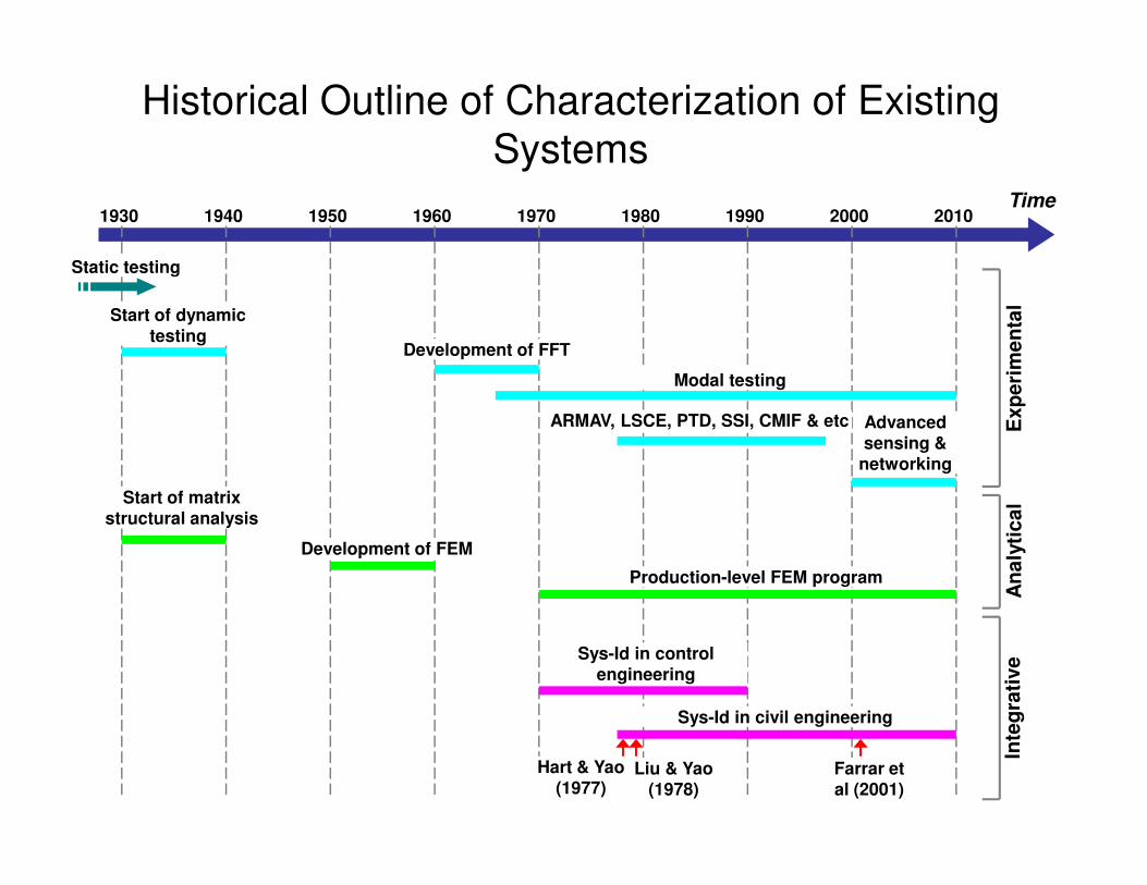
Historical Outline of Characterization of Existing
SystemsTime
1930 1940 1950 1960 1970 1980 1990 2000 2010
Start of dynamic testing
Development of FFT
ARMAV, LSCE, PTD, SSI, CMIF & etc Advanced sensing &
Exp
eri
men
tal
Modal testing
Static testing
sensing & networking
Development of FEM
Start of matrix structural analysis
Production-level FEM program
Sys-Id in control engineering
Hart & Yao (1977)
Liu & Yao (1978)
Farrar et al (2001)
Sys-Id in civil engineering
An
aly
tical
Inte
gra
tive
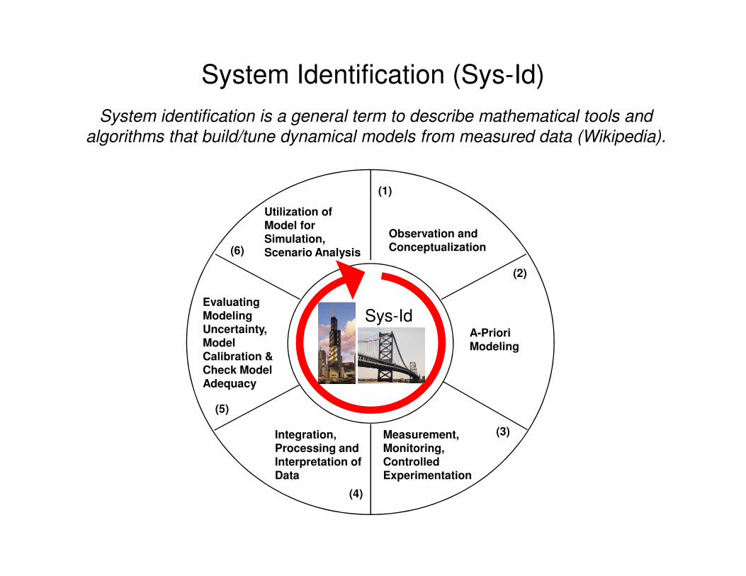
System Identification (Sys-Id)
Utilization of Model for Simulation, Scenario Analysis
Observation and Conceptualization
(2)
(1)
(6)
System identification is a general term to describe mathematical tools and
algorithms that build/tune dynamical models from measured data (Wikipedia).
Sys-IdA-Priori Modeling
Measurement, Monitoring, Controlled Experimentation
Evaluating Modeling Uncertainty, Model Calibration & Check Model Adequacy
Integration, Processing and Interpretation of Data
(4)
(3)
(5)
Outline
� Background & Definition
� Past Research: Sys-Id Applications on Civil Structures
� Research Motivations & Objectives
� Impact of Epistemic Modeling Uncertainty on the Reliability of Sys-IdReliability of Sys-Id
� Recognition & Mitigation of Epistemic Modeling Uncertainty
� Model Adequacy Evaluation
� Conclusions
� Recommendations & Future Work

Suspended SpanCantilever Arm
Cantilever Arm
Anchor Span Anchor Span
822 ft 411 ft 822 ft 411 ft 822 ft
P.P. 27 P.P. 45
Before Retrofit
Commodore Barry Bridge (Grimmelsman 2005)
Pin
Hanger
Cantilever
Arm
Suspended
Span
Ha
ng
er
Pin
Pin
30
m
1
3D FEM of Hanger Region
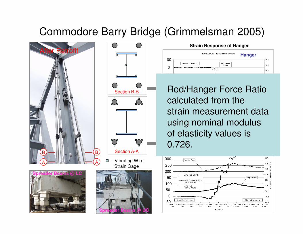
After Retrofit
Commodore Barry Bridge (Grimmelsman 2005)
Section B-B
Hanger100
0
-100
-200
-300
-400
-500
- 600
Strain Response of Hanger
Rod/Hanger Force Ratio
calculated from the
strain measurement data
Spreader Beams @ LC
Spreader Beams @ UC
AA
BB Section A-A
- Vibrating Wire
Strain Gage
Rod400
350
300
250
200
100
50
0
150
-50
Strain Response of Rod
using nominal modulus
of elasticity values is
0.726.

Brooklyn Bridge (Grimmelsman 2006)
0 0.5 1 1.5 2 2.5 3 3.5 4 4.5 50
0.5
1
1.5
2
2.5
3
3.5
4
4.5x 10
-7
Accele
ration (
g2/H
z)
B
C
E
G
H
MT
Tower Longitudinal Vibration Output Spectra
18 Peaks in 0-5 Hz Band
V TLL V
TLTLTL
TLTLTL
TLL
TLL
TLL
V V
V V
V V
L L
L L L
L L L
L
L
L
L
L
L
T
T
T
T
T
T
T
TT
T
Measures to rule out spurious results:
• Max MIF
• Shape Plausibility
• Shape agreement
• Coherence
• MAC values
• Phase factor
• Span modes
0 0.5 1 1.5 2 2.5 3 3.5 4 4.5 5
Frequency (Hz)
?
Mechanically Transparent System
Conceptualized Analytical model
V VV V
1.387 Hz
0
50
100
150
200
250
-1.0 -0.5 0.0 0.5 1.0
Blong
Clong
Elong
Glong
Hlong
the 1st longitudinal tower mode f = 1.387 Hz
-1.0 -0.5 0.0 0.5 1.0
1.201
1.294
1.387
1.450
1.519
0.313
0.381
0.439
0.566
0.610
0.806
0.972
1.201
1.294
1.387
1.450
1.519
Unit Normalized Modal Amplitude

Demonstrator @ Di3 Lab (Ciloglu 2006)
Reduced-Scaled Deck-on-Beam Bridge Model
Relationship btw Major Sources of Uncertainty & Identified Experimental Modal Parameters
Connections Boundary
Post-processingPreprocessingStructural
Complexity Excitation
Steel Roller
SubstructureNot Distributed
Random Dec.
W/o Exp. Window
Signal L-2
DFT CMIF
PTD
SSI
Correlation Func.
Signal L-1
Signal L-3
W/ Exp. Window
SignalModeling
Steel Roller+ Weight
Neoprene Roller
SuperstructureDistributed
SuperstructureNot Distributed
SubstructureDistributed
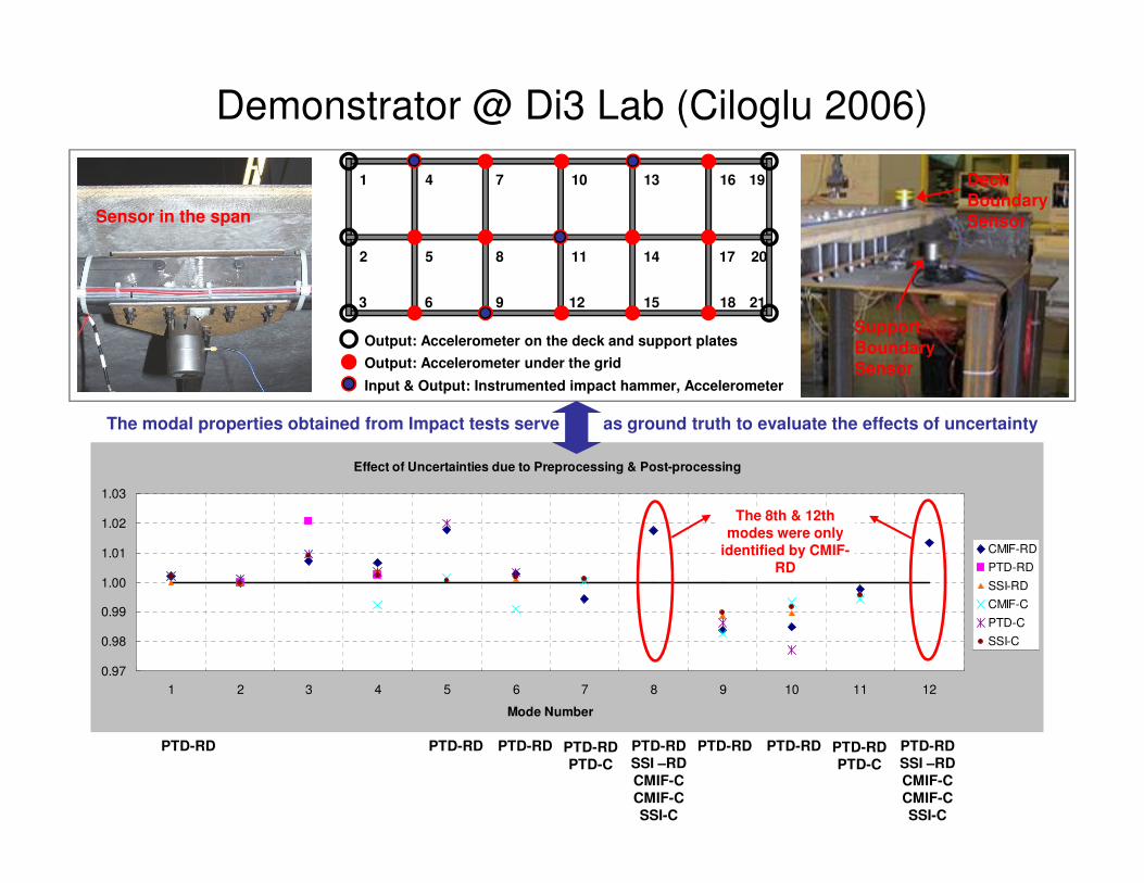
Demonstrator @ Di3 Lab (Ciloglu 2006)
Support Boundary Sensor
Deck Boundary SensorSensor in the span
1 4 7 10 13 16 19
5 8 11 14 17
3 6 9 12 15 18 21
2 20
Output: Accelerometer on the deck and support plates
Output: Accelerometer under the grid
Input & Output: Instrumented impact hammer, Accelerometer
The modal properties obtained from Impact tests serve as ground truth to evaluate the effects of uncertainty
Effect of Uncertainties due to Preprocessing & Post-processing
0.97
0.98
0.99
1.00
1.01
1.02
1.03
1 2 3 4 5 6 7 8 9 10 11 12
Mode Number
CMIF-RD
PTD-RD
SSI-RD
CMIF-C
PTD-C
SSI-C
The 8th & 12th modes were only
identified by CMIF-RD
PTD-RD PTD-RD PTD-RD PTD-RDPTD-C
PTD-RDSSI –RDCMIF-CCMIF-CSSI-C
PTD-RD PTD-RD PTD-RDPTD-C
PTD-RDSSI –RDCMIF-CCMIF-CSSI-C

Outline
� Background & Definition
� Past Research: Sys-Id Applications on Civil Structures
� Research Motivations & Objectives
� Impact of Epistemic Modeling Uncertainty on the Reliability of Sys-IdReliability of Sys-Id
� Recognition & Mitigation of Epistemic Modeling Uncertainty
� Model Adequacy Evaluation
� Conclusions
� Recommendations & Future Work

Motivation: Lessons from Past Experience
� Significant obstacles for widespread implementations of Sys-Id in engineering practice primarily stem from our inability to reliably simulate, measure and interpret the actual physical behaviors of a constructed system, consequently leading to the skepticism towards the credibility of Sys-Id held by owners/stewards of constructed systems.
� These limitations mainly arise from various sources of uncertainty which smear into Sys-Id process through the choice of model structure, idealization of boundary and continuity conditions as well as the design, idealization of boundary and continuity conditions as well as the design, execution and interpretation of field testing and monitoring program.
� Current applications of Sys-Id usually lump uncertainties inherent in a constructed system as a small number of incorrect model parameters or random variables with assumed probability models.
� Many sources of uncertainty, as demonstrated in previous examples, stem from those unknown or less understood structural behaviors as well as their interactions with surrounding environments. They are difficult to be described with probability models and in some cases they may even not be parameterized.
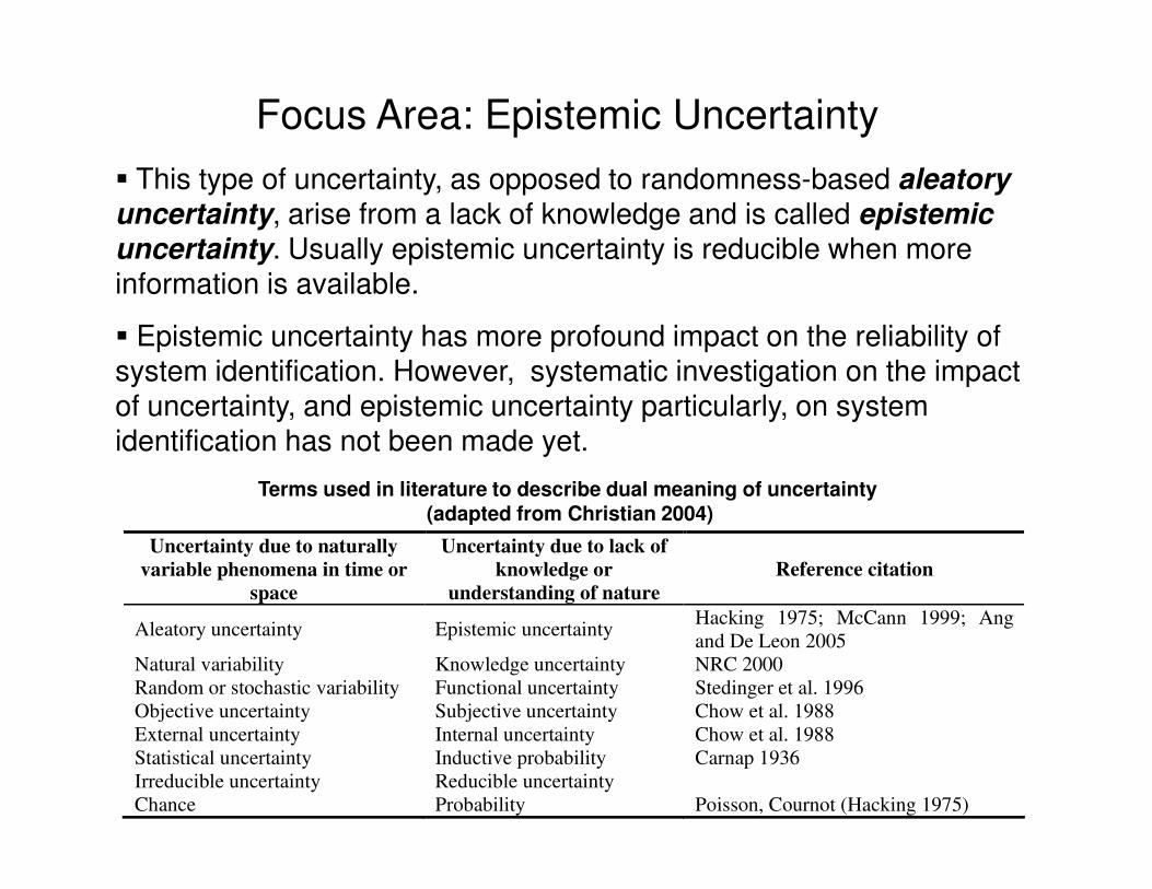
� This type of uncertainty, as opposed to randomness-based aleatory
uncertainty, arise from a lack of knowledge and is called epistemic
uncertainty. Usually epistemic uncertainty is reducible when more information is available.
� Epistemic uncertainty has more profound impact on the reliability of system identification. However, systematic investigation on the impact of uncertainty, and epistemic uncertainty particularly, on system identification has not been made yet.
Focus Area: Epistemic Uncertainty
identification has not been made yet.
Terms used in literature to describe dual meaning of uncertainty(adapted from Christian 2004)
Uncertainty due to naturally
variable phenomena in time or
space
Uncertainty due to lack of
knowledge or
understanding of nature
Reference citation
Aleatory uncertainty Epistemic uncertainty Hacking 1975; McCann 1999; Ang
and De Leon 2005
Natural variability Knowledge uncertainty NRC 2000
Random or stochastic variability Functional uncertainty Stedinger et al. 1996
Objective uncertainty Subjective uncertainty Chow et al. 1988
External uncertainty Internal uncertainty Chow et al. 1988
Statistical uncertainty Inductive probability Carnap 1936
Irreducible uncertainty Reducible uncertainty
Chance Probability Poisson, Cournot (Hacking 1975)

ACTUAL STATE OF A CONSTRUCTED SYSTEM: M, K, C
CONVERGED SYS-ID
RESULTS
Epistemic Uncertainty
DIVERGED SYS-ID
RESULTS
CONVERGED SYS-ID
RESULTS
Additional Information
Additional Information
Epistemic Uncertainty
1
26
START OF SYS-ID
Gro
un
d t
ruth
Aleatory Uncertainty
Aleatory Uncertainty
Aleatory Uncertainty
Sys-Id
Aleatory Uncertainty
2
3
6
4
5
Gro
un
d t
ruth

(3) Controlled Experimentation
STRUCTURAL COMPLEXITY:
•Non-stationarity of boundary and
continuity conditions
•Changes in intrinsic stresses during
tests (redundancy, deterioration)
•Nonlinearities: Many forms of
material and damping nonlinearity,
friction, intermittent contact and uplift
FORCE AND EXCITATION:•Amplitude
•Spectral distribution
•Spatial distribution and
transmissibility
•Directionality
•Dimensionality (1D, 2D or 3D)
•Duration and Non-stationarity
DATA ACQUISITION:•Spatial aliasing
•Time synchronization
•Hardware filtering options
•Noise & bias in signal
•Measurement bandwidth
•Cabling and installation effects
(2) Preliminary Model(s)
•Analytical representation of
physical members and connections
•Completeness of 3D geometry
•Real-time data quality
assessment, management and
warehousing
(4) Data Processing
Sys-Id
•Health/Performance
Monitoring
•Damage detection, Prognosis
•Scenario Analysis and
Vulnerability Assessment
•Performance-based
Engineering
•Guidelines and Codes
(6) Utilization(1) Conceptualization
•Identify/Leverage Heuristics
•Archival of structural drawings
/design calculations, inspection
reports
•Site visits, geometry
measurements, photogrammetry
•Material Sampling, testing, NDE
•Virtual Reconstruction in 3D CAD
•Completeness of 3D geometry
•Soil-foundation, structural
members, joints: stiffness and
kinematics
•Mechanisms/Forms of Nonlinearity
•Test-analysis correlation
•Parameter grouping
•Sensitivity Analysis
•Modality
•Objective function and
constraints
•Optimization
•Physical interpretation of results
(5) Model Calibration
warehousing
•Error identification/ Cleaning
•Different filtering, averaging and
windowing options
•Data post-processing algorithmsUncertainty

Research Objectives
� Influence of modeling uncertainty due to epistemic mechanisms on analytical modeling of
constructed systems
� Feasible techniques to recognize and mitigate modeling uncertainty
� Adequacy of a field-calibrated model to simulate � Adequacy of a field-calibrated model to simulate
all of the critical physical mechanisms impacting a
constructed system
� Review of model updating procedures including test-
analysis correlation, error localization, sensitivity
analysis, and data informativeness quantification as
well as updating algorithms.
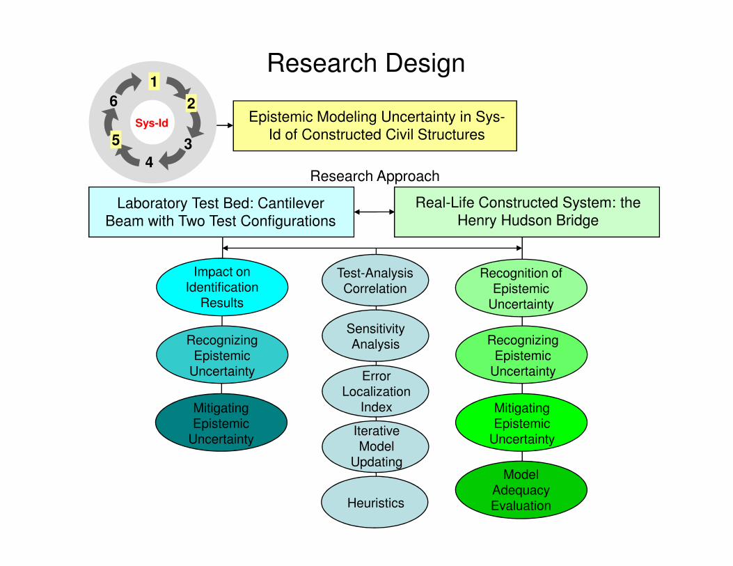
Laboratory Test Bed: Cantilever
Beam with Two Test Configurations
Impact on Identification
Test-Analysis Correlation
Real-Life Constructed System: the
Henry Hudson Bridge
Recognition of Epistemic
Research Design1
2
3
4
5
6Epistemic Modeling Uncertainty in Sys-
Id of Constructed Civil StructuresSys-Id
Research Approach
Identification Results
Recognizing Epistemic
Uncertainty
Mitigating Epistemic
Uncertainty
Model Adequacy Evaluation
Correlation Epistemic Uncertainty
Recognizing Epistemic
Uncertainty
Mitigating Epistemic
Uncertainty
Sensitivity Analysis
Error Localization
Index
Iterative Model
Updating
Heuristics

Outline
� Background & Definition
� Past Research: Sys-Id Applications on Civil
Structures
� Research Motivations & Objectives
� Impact of Epistemic Modeling Uncertainty on the
Reliability of Sys-IdReliability of Sys-Id
� Recognition & Mitigation of Epistemic Modeling
Uncertainty
� Model Adequacy Evaluation
� Conclusions
� Recommendations & Future Work
Cantilever Study

Cantilever Beam Study
Test Configuration 1 Test Configuration 2
Model A Model B

1 2 3 4 5
Time (s)
Fo
rce
117.5 in
Property Value
Density ρ 0.284 lb-f/in3
Young’s Modulus E 29x106 lb-f/in
2
Cross Section Area A 0.954 in2
Moment of Inertia I about weak axis 0.355 in4
Modal Contributions to Simulated Impulse Response functions
Mechanical & Material Properties of the Beam
Analytical Simulation of MRIT
f = 4.910 Hz
f = 30.770 Hz
f = 86.157 Hz
f = 168.846 Hz
f = 279.091 Hz
Simulated Frequency Response functionsModal Parameters Estimated Based on Continuum Theory
( ) ( ) 02
2
2
2
2
2
=
∂
∂
∂
∂+
∂
∂
x
uxEI
xt
uxm
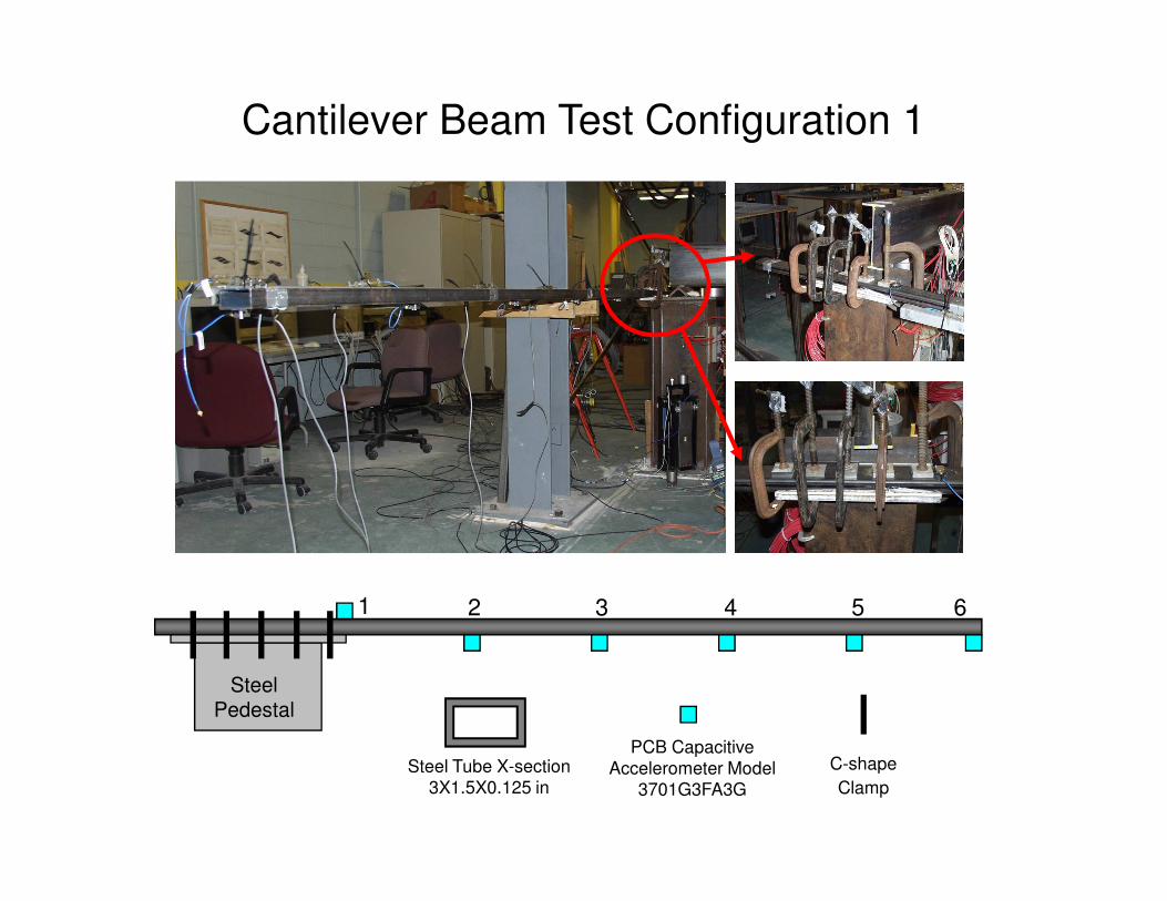
Cantilever Beam Test Configuration 1
1 2 3 4 5 6
Steel Tube X-section
3X1.5X0.125 in
PCB Capacitive
Accelerometer Model
3701G3FA3G
C-shape
Clamp
Steel Pedestal

Cantilever Beam Test Configuration 2
C
B
A
D
12 3 4 5 6
Steel Pedestal
24x3x3/4 in steel plate; center to center
distance btw two rods connected on the
same plate is 18 inch
4-inch long aluminum angle L6x6x3/8 in
A
B
High-strength steel rod with d = 3/8 inch
16-inch long steel angle L3x3x1/2 in
C
D
Steel Tube X-section
3X1.5X0.125 in
PCB Capacitive
Accelerometer Model
3701G3FA3G
C-shape
Clamp

Impact Test
VXI DAC Express Software
Agilent IO Lib Control
DAQ PC
DAQ PC
HPVXI
Data Acquisition Diagram
Impact Excitation
HP VXI
ImpulseHammer 086C02
Microdot cable
Co-ax cable
Breakout box PCB 3701G3FA3G Capacitive Accelerometers
Ch1
Ch2
Ch3
Ch4Ch5
Ch6
Ch 7
Impact Force
FRF
Test Measurements

1
2 3 4 5 6
STATIC LOAD @ PT 5
Celesco PT101 cable-extension transducer
PCB 3701G3FA3G capacitive accelerometer
Static Test
Time-History Displacement Response of the beam
Static Test Sensor Layout
CELESCO PT101
MODE 3
1.2
MODE 2
-0.8
-0.4
0.0
0.4
0.8
1.2
0.0000 20.0000 40.0000 60.0000 80.0000 100.0000 120.0000
Distance (in)
MODE 1
0.0
0.2
0.4
0.6
0.8
1.0
0.0000 20.0000 40.0000 60.0000 80.0000 100.0000 120.0000
Distance (in)
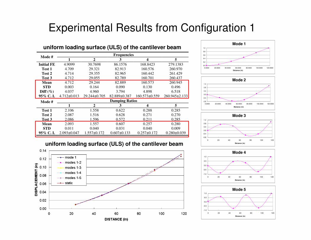
Experimental Results from Configuration 1
Frequencies Mode #
1 2 3 4 5
Initial FE 4.9099 30.7698 86.1576 168.8423 279.1383
Test 1 4.709 29.321 82.913 160.576 260.970
Test 2 4.714 29.355 82.965 160.442 261.429
Test 3 4.712 29.055 82.789 160.701 260.437
Mean 4.712 29.244 82.889 160.573 260.945
STD 0.003 0.164 0.090 0.130 0.496
Diff (%) 4.037 4.960 3.794 4.898 6.518
95% C. I. 4.712±0.013 29.244±0.705 82.889±0.387 160.573±0.559 260.945±2.133
Damping Ratios Mode # 1 2 3 4 5
Test 1 2.106 1.558 0.622 0.288 0.285
Test 2 2.087 1.516 0.628 0.271 0.270
Test 3 2.086 1.596 0.572 0.211 0.285
Mode 1
Mode 2
Mode 3
uniform loading surface (ULS) of the cantilever beam
MODE 5
-1.0
-0.5
0.0
0.5
1.0
0 20 40 60 80 100 120
Distance (in)
MODE 4
-1.0
-0.5
0.0
0.5
1.0
0 20 40 60 80 100 120
Distance (in)
-0.8
-0.4
0.0
0.4
0.8
1.2
0 20 40 60 80 100 120
Distance (in)
X- Modal
Test 3 2.086 1.596 0.572 0.211 0.285
Mean 2.093 1.557 0.607 0.257 0.280
STD 0.011 0.040 0.031 0.040 0.009
95% C. I. 2.093±0.047 1.557±0.172 0.607±0.133 0.257±0.172 0.280±0.039
Mode 4
Mode 5
uniform loading surface (ULS) of the cantilever beam
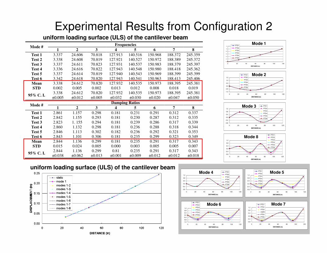
Frequencies Mode #
1 2 3 4 5 6 7 8
Test 1 3.337 24.606 70.818 127.913 140.516 150.968 188.372 245.359
Test 2 3.338 24.608 70.819 127.921 140.527 150.972 188.389 245.372
Test 3 3.337 24.611 70.823 127.931 140.537 150.983 188.379 245.397
Test 4 3.336 24.616 70.822 127.943 140.548 150.980 188.418 245.362
Test 5 3.337 24.614 70.819 127.940 140.543 150.969 188.399 245.399
Test 6 3.342 24.618 70.820 127.943 140.541 150.963 188.413 245.406
Mean 3.338 24.612 70.820 127.932 140.535 150.973 188.395 245.381
STD 0.002 0.005 0.002 0.013 0.012 0.008 0.018 0.019
95% C. I. 3.338
±0.005
24.612
±0.012
70.820
±0.005
127.932
±0.032
140.535
±0.030
150.973
±0.020
188.395
±0.047
245.381
±0.050
Damping Ratios Mode #
1 2 3 4 5 6 7 8
Test 1 2.861 1.157 0.298 0.181 0.231 0.291 0.312 0.337
Test 2 2.842 1.155 0.293 0.181 0.230 0.287 0.312 0.335
Test 3 2.823 1. 155 0.294 0.181 0.239 0.286 0.317 0.339
Test 4 2.860 1.132 0.298 0.181 0.236 0.288 0.318 0.344
Experimental Results from Configuration 2uniform loading surface (ULS) of the cantilever beam
MODE 1
0.0
0.2
0.4
0.6
0.8
1.0
1.2
0 20 40 60 80 100 120
DISTANCE (in)
PTD1
PTD2
PTD3
PTD4
PTD5
PTD6
MODE 2
-1.0
-0.5
0.0
0.5
1.0
1.5
0 20 40 60 80 100 120
DISTANCE (in)
PTD1
PTD2
PTD3
PTD4
PTD5
PTD6
MODE 3
-0.8
-0.4
0.0
0.4
0.8
1.2
0 20 40 60 80 100 120
PTD1
PTD2
PTD3
PTD4
PTD5
PTD6
Mode 1
Mode 2
Mode 3
Test 4 2.860 1.132 0.298 0.181 0.236 0.288 0.318 0.344
Test 5 2.846 1.113 0.302 0.182 0.236 0.292 0.321 0.353
Test 6 2.843 1.101 0.306 0.181 0.235 0.299 0.323 0.349
Mean 2.844 1.136 0.299 0.181 0.235 0.291 0.317 0.343
STD 0.015 0.024 0.005 0.000 0.003 0.005 0.005 0.007
95% C. I. 2.844
±0.038
1.136
±0.062
0.299
±0.013
0.81
±0.001
0.235
±0.009
0.291
±0.012
0.317
±0.012
0.343
±0.018
uniform loading surface (ULS) of the cantilever beam
DISTANCE (in)
MODE 4
-0.8
-0.4
0.0
0.4
0.8
1.2
0 20 40 60 80 100 120
DISTANCE (in)
PTD1
PTD2
PTD3
PTD4
PTD5
PTD6
MODE 5
-0.8
-0.4
0.0
0.4
0.8
1.2
0 20 40 60 80 100 120
DISTANCE (in)
PTD1
PTD2
PTD3
PTD4
PTD5
PTD6
MODE 6
-1.2
-0.8
-0.4
0.0
0.4
0.8
1.2
0 20 40 60 80 100 120
DISTANCE (in)
PTD1
PTD2
PTD3
PTD4
PTD5
PTD6
MODE 7
-0.8
-0.4
0.0
0.4
0.8
1.2
0 20 40 60 80 100 120
DISTANCE (in)
PTD1
PTD2
PTD3
CMIF4
PTD5
PTD6
MODE 8
-0.8
-0.4
0.0
0.4
0.8
1.2
0 20 40 60 80 100 120
DISTANCE (in)
PTD1
PTD2
PTD3
PTD4
PTD5
PTD6
Mode 4 Mode 5
Mode 6 Mode 7
Mode 8

Updating Parameter: E
Identification Results Using Model A
1
2
3
4
5
6
7
8
initial
updated
Frequency before and after calibration in Run 1
270
275
280
285
290
E (
x10
5 p
si)
Change of E with iteration in Run 1
Identification Run 1: Cantilever Beam under Configuration 1
-2
-1
0
1
1 2 3 4 5
MODE
-10
0
10
20
30
40
50
1 2 3 4 5
MODE
initial
updated
1 2 3 4260
265
270
Iterations
1 2 3 4 5180
200
220
240
260
280
300
Iterations
E (
x10
5 p
si)
Frequency before and after calibration in Run 2Change of E with iteration in Run 2
Configuration 1
Identification Run 2: Cantilever Beam under Configuration 2
261.724
194.896
Initial value of Eis 290 (x10^5) psi

Observations & Discussions About Identification
Results Using Initial Model A� All of the five observed vibration modes from the cantilever beam under test configuration 1 could be paired up with the analytical predictions from initial model A.
� The test-analysis correlation were improved after calibration by adjusting the Young’s modulus of steel. With a decrease of less than 10 percent of its nominal value, the difference in natural frequency was under 2 percent. The mode shapes remained because they were independent on the updating parameter. independent on the updating parameter.
� In Run 1, the information in all five modes was included in model updating, while the fourth mode was excluded in identification Run 3. However, the updated values of the model parameter as well as the natural frequencies were very similar.
� A total of eight modes were identified from the beam under test configuration 2. The first three and the eighth mode were paired up with the analytical first three and the fifth mode from initial model. The rest four experimental modes all demonstrate deflection shapes similar to the analytical fourth bending mode.
� Immense uncertainty was associated with the correlation between the measured and simulated fourth bending mode. Only four pairs of modes were thus included in identification Run 2.
� Although the gap in natural frequency between the analytical model and experiment observation narrowed considerably after updating, relatively large difference remained, especially in the natural frequency of the first mode.
Observations & Discussions About Identification
Results Using Initial Model A (Cont’d)
frequency of the first mode.
� The calibration process forced the pre-selected updating parameter to decrease by about 33 percent of its initial (nominal) value, which already lost its physical meaning.
� Significant discrepancy was observed in the estimated values for the model parameter E from the identification cases of configurations 1 and 2, which were supposed to converge to the same value because they represented the material property of the same beam.
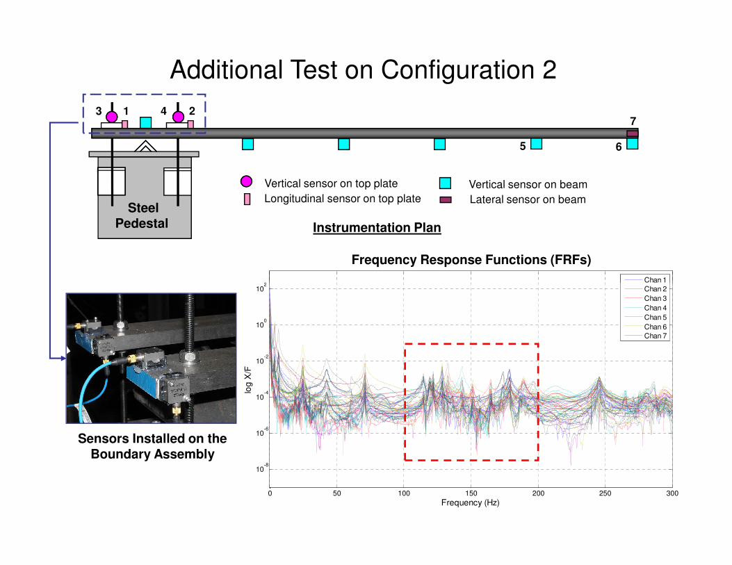
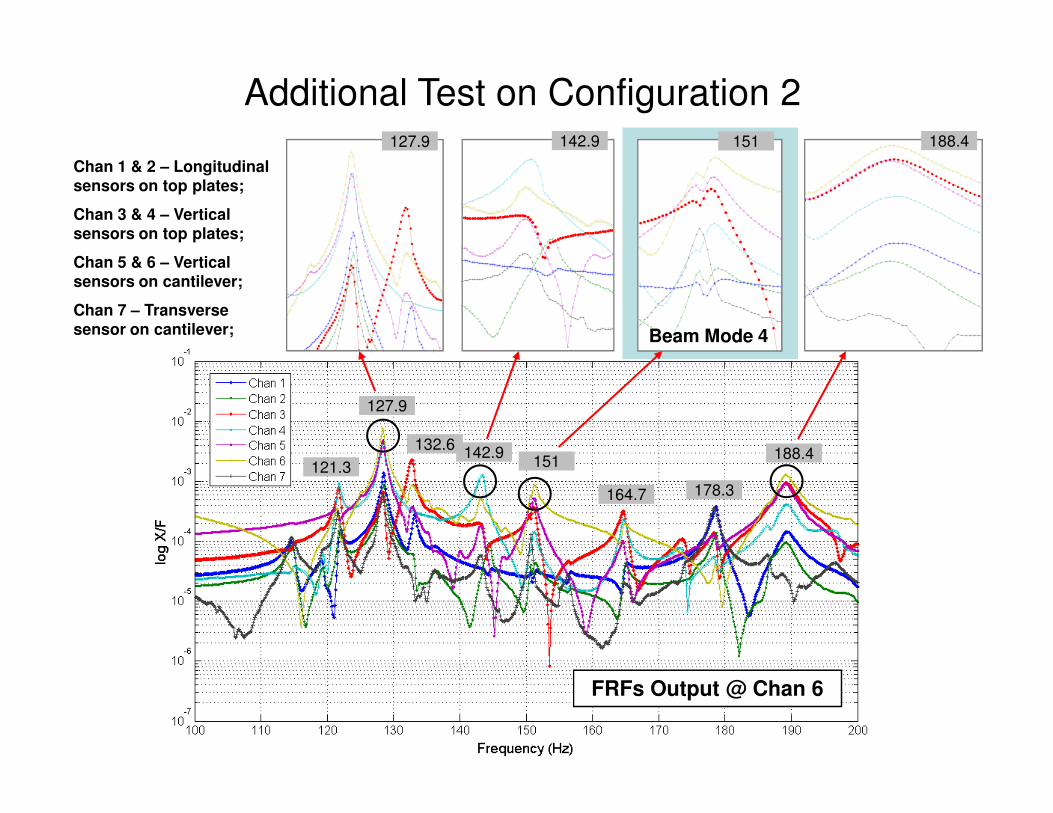
Additional Test on Configuration 2
5
Vertical sensor on top plate
Longitudinal sensor on top plate Lateral sensor on beam
Vertical sensor on beam
6
741 23
SteelPedestal Instrumentation Plan
2
Chan 1
Frequency Response Functions (FRFs)
Sensors Installed on the Boundary Assembly
0 50 100 150 200 250 300
10-8
10-6
10-4
10-2
100
102
Frequency (Hz)
log
X/F
Chan 1
Chan 2
Chan 3
Chan 4
Chan 5
Chan 6
Chan 7
127.9
127.9 142.9 151 188.4
Chan 1 & 2 – Longitudinal sensors on top plates;
Chan 3 & 4 – Vertical sensors on top plates;
Chan 5 & 6 – Vertical sensors on cantilever;
Chan 7 – Transverse sensor on cantilever;
Additional Test on Configuration 2
Beam Mode 4
FRFs Output @ Chan 6
121.3
127.9
132.6142.9
151
164.7 178.3
188.4

282
284
286
288
290
E (
x10
5 p
si)
Identification Results Using Initial Model B
Frequency before and after calibration in Run 4
Change of E
Updating parameters: E, Kr
0
1
2
3
4
5
initial
updated
460
470
480
490
500
Kr
(x10
4 p
si)
Change of Kr
Identification Run 4: Cantilever Beam under Configuration 1
Initial value of E is 290 (x10^5) psi; Initial value of Kr is 500 (x10^4) psi;
0 5 10 15 20200
210
220
230
240
250
260
270
280
290
Iterations
E (
x10
5 p
si)
0 2 4 6 8 10 12 14 16 18278
280
282
Iterations
Frequency before and after calibration in Run 5
Change of E
-2
-1
1 2 3 4 5
MODE
-5
0
5
10
15
20
25
30
35
40
45
1 2 3 4 5
MODE
initial
updated
0 2 4 6 8 10 12 14 16 18440
450
460
Iterations
Kr
(x10
0 5 10 15 200
100
200
300
400
500
Iterations
Kr
(x10
4 p
si)
Change of Kr
Identification Run 5: Cantilever Beam under Configuration 2
279.603
280.983

MODE 1
0.0
0.2
0.4
0.6
0.8
1.0
0 20 40 60 80 100 120
Distance (in)
test
initial
updated
MODE 2
-0.8
-0.4
0.0
0.4
0.8
1.2
0 20 40 60 80 100 120
Distance (in)
test
initial
updated
MODE 3
-0.8
-0.4
0.0
0.4
0.8
1.2
0 20 40 60 80 100 120
Distance (in)
test
initial
updated
MODE 4
-1.0
-0.5
0.0
0.5
1.0
0 20 40 60 80 100 120
Distance (in)
test
initial
updated
MODE 5
-1.0
-0.5
0.0
0.5
1.0
0 20 40 60 80 100 120
Distance (in)
test
initial
updated
Initial Updated
1 1.0000 1.0000
2 0.9987 0.9988
3 0.9989 0.9989
4 0.9965 0.9966
5 0.9958 0.9958
mode #MAC
Identification Results with Model BBeam with Configuration 1 (Run 4)
Distance (in) Distance (in) 5 0.9958 0.9958
MODE 2
-0.8
-0.4
0
0.4
0.8
1.2
0 20 40 60 80 100 120
DISTANCE (in)
test
initial
updated
MODE 4
-0.8
-0.4
0
0.4
0.8
1.2
0 20 40 60 80 100 120
DISTANCE (in)
test
initial
updated
MODE 3
-0.8
-0.4
0
0.4
0.8
1.2
0 20 40 60 80 100 120
DISTANCE (in)
test
initial
updated
MODE 5
-0.8
-0.4
0
0.4
0.8
1.2
0 20 40 60 80 100 120
DISTANCE (in)
test
initial
updated
MODE 1
0
0.2
0.4
0.6
0.8
1
1.2
0 20 40 60 80 100 120
DISTANCE (in)
test
initial
updated
initial updated
1 0.9941 1.0000
2 0.9831 0.9996
3 0.9604 0.9972
4 0.9849 0.9949
5 0.9759 0.9959
Mode #MAC
Beam with Configuration 2 (Run 5)

Observations & Discussions
� Additional dynamic test on the beam with configuration 2 revealed the interaction between the beam and boundary assembly. This observation was conceptualized as rotational spring at the beam support in initial model B.
� Among the four modes which demonstrated similar deflection shapes, f = 150.99 Hz was dominated by the vibrations of the beam and was only included in the calibration process.
� With initial model B, the beam under two test configuration 1 and 2 were calibrated in identification Run 4 and 5 respectively. In Run 4, the calibrated model converged to the similar level as that in Run 1 and 3. In Run 5 the discrepancy between the predicted natural frequencies and their experimental counterparts were significantly reduced and only ±3 percent difference remained.
� The values for the common model parameter in Run 4 and 5, the Young’s modulus E, both decreased by about 3 percent of its nominal value, although they did not converge to the exact same value.

Observations & Discussions
� Good correlation between the values of common updated parameter as well as the modal predictions implied that the initial model Befficiently conceptualize the influences of the rotary movement of the boundary assembly on the beam without explicitly incorporating the boundary assembly in the initial model.
� Epistemic modeling uncertainty associated with the initial model Awould seriously impair the reliability of the identification for the beam under configuration 2.
Updating
Parameter Nominal
Run 1: Config 1
with model A
Run 2: Config 2
with model A
Run 4: Config 1
with model B
Run 5: Config 2
with model B
E (×105 psi) 290 261.724 194.896 279.603 280.983
Diff (%) -9.750 -32.795 -3.585 -3.109
under configuration 2.
� The selected updating parameter tended to compensate for the influence of epistemic modeling error by distorting itself. As a result, the updated value for E lost its physical significance. The calibrated model still failed to accurately predict the experimental frequencies.

Outline
� Background & Definition
� Past Research: Sys-Id Applications on Civil
Structures
� Research Motivations & Objectives
� Impact of Epistemic Modeling Uncertainty on the
Reliability of Sys-IdReliability of Sys-Id
� Recognition & Mitigation of Epistemic Modeling
Uncertainty
� Model Adequacy Evaluation
� Conclusions
� Recommendations & Future Work
Henry Hudson Bridge
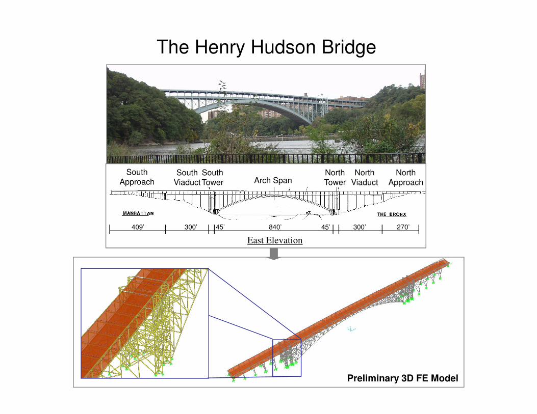
The Henry Hudson Bridge
South
ApproachSouth
Viaduct Arch SpanNorth
Viaduct
North
Approach
South
Tower
North
Tower
East Elevation
300’409’ 45’ 45’ 270’300’840’
Preliminary 3D FE Model
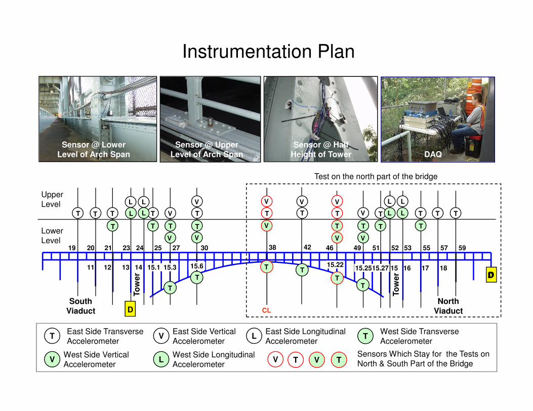
Upper
Level VV VV L LL L
Test on the north part of the bridge
Instrumentation Plan
Sensor @ Lower Level of Arch Span
Sensor @ Upper Level of Arch Span
Sensor @ Half Height of Tower DAQ
D
To
we
r
To
we
r
CL
South Viaduct
North Viaduct
Level
Lower
Level
181716
5957
1515.2715.2515.22
5553525149464238
131211 14 15.1 15.3 15.6
3027252423212019
T T T
T
T
TT
T
T
TT
TT
T
T
T
T
T
T
T
T
T
T
TT
TV
V
V
V
VV
V
VV
V
L L
L L L L
TT
V
VEast Side Vertical
Accelerometer
West Side Vertical
Accelerometer
East Side Transverse
Accelerometer
West Side Transverse
Accelerometer
L
LEast Side Longitudinal
Accelerometer
West Side Longitudinal
AccelerometerV T V T
Sensors Which Stay for the Tests on
North & South Part of the Bridge
D
D

0 200 400 600 800 1000 1200 1400 1600 1800 2000-8
-6
-4
-2
0
2
4
6
8x 10
-3
0 20 40 60 80 100 120-6
-4
-2
0
2
4
6x 10
-7
0 1 2 3 4 5 6 7 8 9 1010
-7
10-6
10-5
10-4
Time-domain measurements under ambient conditions
Pseudo IRF generated by spectrum estimation methods
Pseudo FRF generated by spectrum estimation methods
Imported in X-Modal and process with PTD
Stability plot to present consistency of poles with different model order
Modal Parameters:
Preprocessing
Data Analysis
• Stationarity
Check;
• Effect of Traffic Load Amplitude;
• Effect of
Sampling
Bandwidth;
Data Processing
Imported in X-Modal and process with CMIF
CMIF plot generated based on singular value decomposition
Modal Parameters: ω, ζ, Φ
Post-processing by CMIFPost-processing by PTD
-200
0
200
400
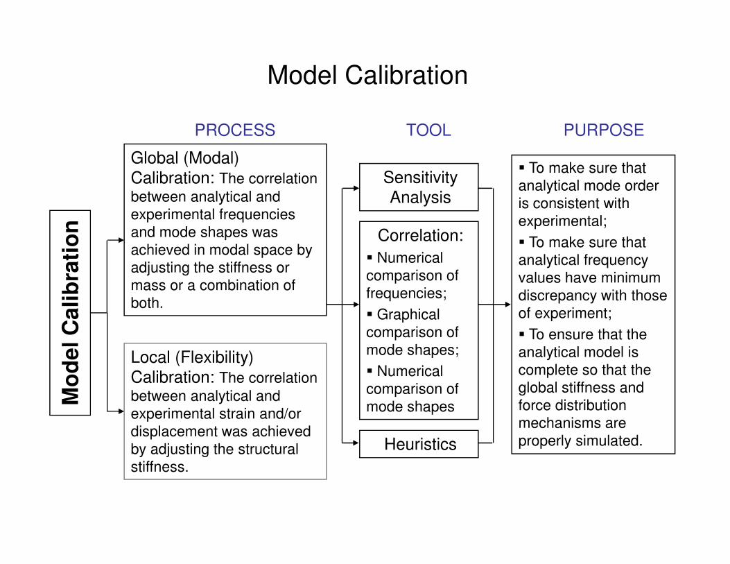
Model Calibration
Global (Modal)
Calibration: The correlation
between analytical and
experimental frequencies
and mode shapes was
achieved in modal space by
adjusting the stiffness or
mass or a combination of
Mo
del C
ali
bra
tio
n
Sensitivity
Analysis
Correlation:
� Numerical
comparison of
� To make sure that
analytical mode order
is consistent with
experimental;
� To make sure that
analytical frequency
values have minimum
PROCESS TOOL PURPOSE
mass or a combination of
both.
Local (Flexibility)
Calibration: The correlation
between analytical and
experimental strain and/or
displacement was achieved
by adjusting the structural
stiffness.
Mo
del C
ali
bra
tio
n
comparison of
frequencies;
� Graphical
comparison of
mode shapes;
� Numerical
comparison of
mode shapes
Heuristics
values have minimum
discrepancy with those
of experiment;
� To ensure that the
analytical model is
complete so that the
global stiffness and
force distribution
mechanisms are
properly simulated.
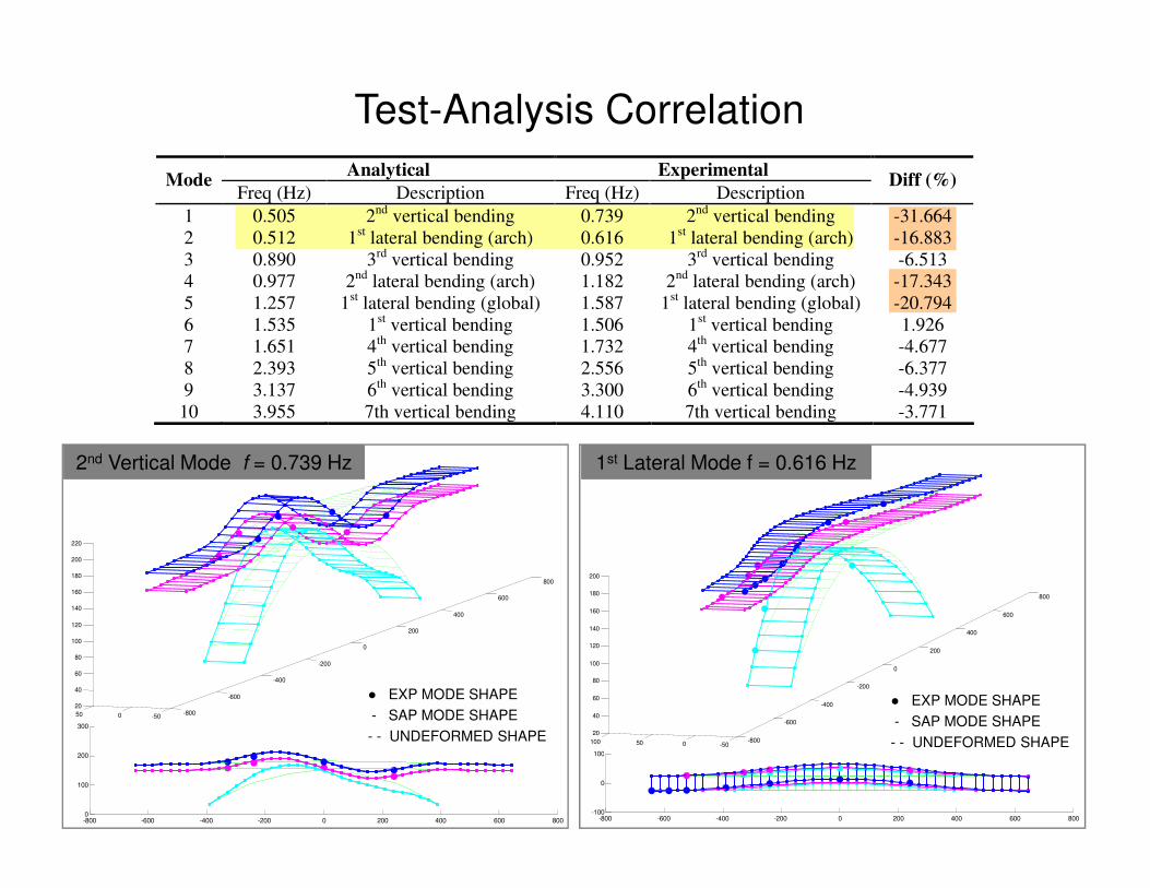
Test-Analysis Correlation
Analytical Experimental Mode
Freq (Hz) Description Freq (Hz) Description Diff (%)
1 0.505 2nd vertical bending 0.739 2nd vertical bending -31.664
2 0.512 1st lateral bending (arch) 0.616 1st lateral bending (arch) -16.883
3 0.890 3rd vertical bending 0.952 3rd vertical bending -6.513
4 0.977 2nd lateral bending (arch) 1.182 2nd lateral bending (arch) -17.343
5 1.257 1st lateral bending (global) 1.587 1st lateral bending (global) -20.794
6 1.535 1st vertical bending 1.506 1st vertical bending 1.926
7 1.651 4th vertical bending 1.732 4th vertical bending -4.677
8 2.393 5th vertical bending 2.556 5th vertical bending -6.377
9 3.137 6th vertical bending 3.300 6th vertical bending -4.939
10 3.955 7th vertical bending 4.110 7th vertical bending -3.771
-800
-600
-400
-200
0
200
400
600
800
-50050
20
40
60
80
100
120
140
160
180
200
220
-800 -600 -400 -200 0 200 400 600 8000
100
200
300
● EXP MODE SHAPE
- SAP MODE SHAPE
- - UNDEFORMED SHAPE -800
-600
-400
-200
0
200
400
600
800
-50050100
20
40
60
80
100
120
140
160
180
200
-800 -600 -400 -200 0 200 400 600 800-100
0
100
● EXP MODE SHAPE
- SAP MODE SHAPE
- - UNDEFORMED SHAPE
2nd Vertical Mode f = 0.739 Hz 1st Lateral Mode f = 0.616 Hz

Sensitivity Analysis
The model parameters/conditions selected for sensitivity analysis include:
� The Young’s modulus of the steel;
� The Young’s modulus of the deck concrete;
� Variations in boundary conditions;
� The continuity conditions between viaduct-deck-arch interface at both the upper and lower decks;
� The stiffness of the lateral translational springs located at each end of the two viaduct spans;
1.8 1.8
0.4
0.6
0.8
1
1.2
1.4
1.6
1.8
0.85 E 0.90 E 0.95 E 1.00 E 1.05 E 1.10 E 1.15 E
Variation of E of Steel
Mo
dal
Fre
qu
en
cy (
Hz)
Mode 1
Mode 2
Mode 3
Mode 4
Mode 5
Mode 6
Mode 7
Mode 8
Mode 9
Mode 10
Mode 11
Mode 12
Mode 13
Mode 14
Mode 15
0.4
0.6
0.8
1
1.2
1.4
1.6
1.8
Equal Constraint in
Uy, Uz
Body Constraint in
Uy, Uz
Body Constraint in
Uy, Uz, Rx, Ry &
Rz
Body Constraint in
all Six DOFs
Variation of Continuity Condition at Deck-Tower Interface
Mo
dal
Fre
qu
en
cy (
Hz)
Mode 1
Mode 2
Mode 3
Mode 4
Mode 5
Mode 6
Mode 7
Mode 8
Mode 9
Mode 10
Mode 11
Mode 12
Mode 13
Mode 14
Mode 15

Heuristics for Calibration
� Correct joint constraints btw arch rib &lower deck;
� Remove frame end releases for vertical members btw arch rib & lower deck;
� Adjust joint rigidity factors at
column-floor connections
� Adjust the continuity conditions at the arch-tower-viaduct interface

Calibration Results
0.9
MA
C V
alu
es o
f V
ert
ical M
odes
Mode
#
Experimental
(Hz)
Initial
(Hz) Diff (%)
Updated
(Hz) Diff (%) Description
1 0.616 0.512 -16.883 0.588 -4.545 1st lateral bending (arch)
2 0.739 0.505 -31.664 0.721 -2.436 2nd vertical bending
3 0.952 0.890 -6.513 0.973 2.206 3rd vertical bending
4 1.182 0.977 -17.343 1.054 -10.829 2nd lateral bending (arch)
5 1.506 1.257 -16.534 1.404 -6.773 1st lateral bending (global)
6 1.587 1.535 -3.277 1.566 -1.323 1st vertical bending
7 1.732 1.651 -4.677 1.714 -1.039 4th vertical bending
8 2.556 2.393 -6.377 2.505 -1.995 5th vertical bending
9 3.300 3.137 -4.939 3.276 -0.727 6th vertical bending
10 4.110 3.955 -3.771 4.061 -1.192 7th vertical bending
1
2
3
4
1
2
3
4
0
0.2
0.4
0.6
0.8
1
0.1
0.2
0.3
0.4
0.5
0.6
0.7
0.8
0.9
1
2
3
4
1
2
3
4
0
0.2
0.4
0.6
0.8
1
0.1
0.2
0.3
0.4
0.5
0.6
0.7
0.8
MA
C V
alu
es o
f V
ert
ical M
odes
Befo
reA
fter
Befo
reA
fter
MA
C V
alu
es o
f Late
ral M
odes

Model Adequacy Check By Sensitivity Analysis of E
NORM OF ERROR IS DEFINED AS: ∑=
−=
7
1
2
i EXPi
EXPiFEi
FREQ
FREQFREQNORM
VERTICAL FREQUENCIES & NORMS OF ERROR (Hz) FROM INITIAL MODEL
MODE # 0.85 E 0.90 E 0.95 E 1.00 E 1.05 E 1.10 E 1.15E 1.20 E 1.25 E EXP
1 0.4660 0.4795 0.4925 0.5053 0.5177 0.5298 0.5416 0.5532 0.5645 0.739
2 0.8204 0.8441 0.8671 0.8895 0.9114 0.9328 0.9537 0.9741 0.9941 0.952
3 1.4152 1.4561 1.4958 1.5345 1.5723 1.6091 1.6451 1.6804 1.7149 1.506
4 1.5234 1.5671 1.6096 1.6510 1.6913 1.7307 1.7692 1.8068 1.8437 1.732
5 2.2083 2.2716 2.3332 2.3931 2.4515 2.5086 2.5643 2.6182 2.6724 2.5560.3
0.4
0.5
0.6
No
rm o
f E
rro
r
UPDATED
INITIAL
VERTICAL FREQUENCIES & NORMS OF ERROR (Hz) FROM UPDATED MODEL
6 2.8965 2.9789 3.0589 3.1369 3.2128 3.2868 3.3592 3.4298 3.4989 3.300
7 3.6551 3.7579 3.8578 3.9549 4.0495 4.1416 4.2303 4.3151 4.4086 4.110
NORM 0.4684 0.4190 0.3754 0.3389 0.3108 0.2927 0.2855 0.2893 0.3034
DIVERGENCE DIVERGENCE
DIVERGENCE DIVERGENCE
MODE # 0.85 E 0.90 E 0.95 E 1.00 E 1.05 E 1.10 E 1.15E EXP
1 0.6723 0.6889 0.7050 0.7207 0.7360 0.7510 0.7656 0.739
2 0.8981 0.9237 0.9486 0.9729 0.9966 1.0196 1.0422 0.952
3 1.4445 1.4862 1.5268 1.5663 1.6048 1.6424 1.6792 1.506
4 1.5852 1.6294 1.6723 1.7141 1.7556 1.7949 1.8337 1.732
5 2.3128 2.3787 2.4428 2.5052 2.5659 2.6252 2.6832 2.556
6 3.0259 3.1114 3.1945 3.2755 3.3543 3.4312 3.5064 3.300
7 3.7531 3.8587 3.9612 4.0610 4.1582 4.2531 4.3457 4.110
NORM 0.2091 0.1449 0.0883 0.0583 0.0844 0.1355 0.1914
0.0
0.1
0.2
0.3
0.8 0.85 0.9 0.95 1 1.05 1.1 1.15 1.2 1.25 1.3
x E
No
rm o
f E
rro
r

Observations & Discussion
� It is feasible to apply integrative paradigm of system identification on large-scale complex structures such as the long-span steel arch bridge.
� Before identifying model uncertainty, it is important to understand uncertainty due to experiment/data processing. The stationarity of recorded data, as well as the effect of the traffic load amplitude and sampling frequency bandwidth on the identified modal parameters sampling frequency bandwidth on the identified modal parameters was carefully examined to exclude possible epistemic measurement uncertainty.
� Global calibration in modal space was conducted based on: (1) Heuristics; (2) test-analysis correlation, and, (3) sensitivity analysis. The calibrated model was shown to accurately predict the modal properties of the bridge in the vertical direction. The test-analysis correlation in lateral direction is not as good most likely due to a lack
of sufficient excitation in the lateral direction.
Observations & Discussion (Cont’d)
� The sensitivity of the modal parameters with respect to the elasticity modulus of the steel was leveraged to assess the adequacy of the field-calibrated model.
� The level of discrepancy was significantly decreased after calibration: The elasticity modulus decreased after calibration: The elasticity modulus converged around its nominal value, which indicated the calibrated model was the most admissible model given the available information.

Conclusions: Impact of Epistemic Modeling Uncertainty
� Epistemic modeling uncertainty is usually closely related to the choice of model form, element type, idealization of geometry, material properties as well as boundary and continuity conditions.
� In real-life applications of system identification, epistemic modeling uncertainty is coupled with other sources of uncertainty. Its impacts propagate and manifest this phenomenon in various ways as identification progresses from Step 2 on.
� Compared with aleatory modeling uncertainty which may affect the � Compared with aleatory modeling uncertainty which may affect the accuracy of model parameters, the modeling uncertainty due to epistemic mechanisms could lead to divergence in identification results (large test-analysis discrepancy may remain the calibrated model, and/or the updated parameters may lose their physical significance).
� Epistemic modeling uncertainty may cause those updating parameters associated with little random variability (e.g Es) to appear as if they are the dominant uncertainty sources. In this study when there was epistemic modeling uncertainty, Es exhibited large variations during the updating process in order to compensate for the test-analysis discrepancy.

Conclusions: Recognition & Mitigation of
Epistemic Modeling Uncertainty
� The abnormality of the updated value for the elasticity modulus of steel in the cantilever investigation served as a good indicator for the presence of unacknowledged epistemic modeling uncertainty in analytical model.
� Therefore a feasible and effective indicator for the presence of epistemic modeling uncertainty associated with the a priori model of a constructed system was to incorporate into updating procedure one or constructed system was to incorporate into updating procedure one or more of the global model parameters of little known variability. If these appear to be sensitive to the change of dynamic properties, we will use this to identify the presence of epistemic model uncertainty.
� Most effective solution to reduce epistemic uncertainty is to obtain additional information about the system and fully leverage heuristics. The additional dynamic test on the configuration 2 of the cantilever revealed the interactions between the beam and boundary assembly.

Conclusions: Evaluating Model Adequacy
� System identification paradigm is a powerful tool to characterize the actual behaviors of a constructed system and it is feasible to be used on large-scale complex civil engineering structures.
� In real-life applications, systematical utilization of engineering heuristics often played a critical role in reducing modeling uncertainty and epistemic modeling uncertain in particular embedded in the a priori model of the structure.
� The sensitivity analysis of the model properties predicted by analytical � The sensitivity analysis of the model properties predicted by analytical models before and after calibration with respect to the elasticity modulus of steel indicated that the field-calibrated model of the bridge was the most admissible one with available information.
� With limited information embedded in available test data, it is often extremely difficult to determine an unique and converged calibrated model. The proposed model adequacy evaluation tool was intended to assist in checking whether critical physical mechanisms of the system under study were properly incorporated in the analytical model.

� A feasible technique to recognize epistemic modeling uncertainty in the analytical model are proposed in the thesis. This idea could be further investigated with designed laboratory tests and candidates for the dummy model parameters should also include global and sensitive parameters such as the mass of the system or a subsystem.
� Additional research is required in order to better pinpoint the sources of epistemic modeling uncertainty. This would lead to more efficient
Recommendations & Future Work
of epistemic modeling uncertainty. This would lead to more efficient mitigation of epistemic modeling uncertainty.
� A stochastic framework should be incorporated into the system identification paradigm.
� The global calibration which mainly takes advantage of modal data from vibration tests should be utilized in conjunction with local calibration based on static data from load tests.

Thank You
Recommended