SUPERFLUID HYDROGEN IN NANOSCALE
CONFINEMENT
by
Tokunbo P. Omiyinka
A thesis submitted in partial fulfillment of the requirements for the degree of
Master of Science
Department of Physics
University of Alberta
© Tokunbo P. Omiyinka, 2014

Abstract
Confinement is known to suppress order in condensed matter. This is well
exemplified in phase transitions such as freezing, as well as the superfluid
transition in liquid helium, which occur at lower temperatures in confinement
than in the bulk. We provide in this thesis a demonstration of a physical
setting in which the reverse takes place. Particularly, the enhancement of
the superfluid response of parahydrogen confined to nanoscale size cavities
is illustrated by means of first principle computer simulations. Prospects to
stabilize and observe the long investigated but yet elusory bulk superfluid
phase of parahydrogen in objectively designed porous media are discussed.
ii
Preface
The entirety of this thesis constitute the original thesis research of Tokunbo
Omiyinka, under the supervision of Professor Massimo Boninsegni.
Chapter 3 of this work has been published as: Tokunbo Omiyinka and Mas-
simo Boninsegni, “Pair potentials and equation of state of solid para-hydrogen
to megabar pressure”, Physical Review B 88, 024112 (2013).
Also, Chapter 4 has been published as: Tokunbo Omiyinka and Massimo
Boninsegni, “Enhanced superfluid response of parahydrogen in nanoscale con-
finement”, Physical review B 90, 064511 (2014).
iii

Acknowledgements
I am immensely grateful for having the opportunity to pursue my graduate
studies at the University of Alberta. I am profoundly indebted to my super-
visor, Prof. Massimo Boninsegni, who is responsible for every inch of success
in my masters program and in making this thesis a reality. I am particularly
thankful for your unrelenting dedication to constantly guide me through vari-
ous learning curves, making it possible for me to achieve things I would have
thought impossible. Thank you very much.
I also like to appreciate Prof. Kevin Beach whose support and recommen-
dations were crucial to the start of my graduate studies. Many thanks to
you.
To Sarah Derr, for your kindness in being always ready to guide and assist
countless graduate students, including myself, I say a huge thank you.
To Gordon and Carol Buzikevich, your unrelenting support in every possi-
ble way, as well as your staying close to my family through our successes and
challenges, are inestimable and worthy of unending thanks; thanks a great
deal.
I am also very thankful to Kingsley Emelideme, Burkhard Ritter, Ebele
Ezeokafor and Godfrey Obumneme for your enduring support in many ways.
I also like to express my deep gratitude to many others whose varying support,
encouragement and criticism contribute to the success of my masters degree.
To my most beloved parents (of blessed memory), Mr & Mrs. Akinposi and
Adija Omiyinka, and my wonderful siblings (Bukola, Folake, Daniel, Goodness,
Samuel and Testimony), I am full of thanks and inexpressible appreciation for
iv

your relentless prayers and faith in me. I love you all. Uncle Muhammed
Omisore, your prayers and best wishes go a long way in assisting me in my
studies; thank you very much.
My dearest wife, ayanfemi, Oluwabukolami, your support, prayers, under-
standing, affection and love are sources of renewed life, strength and hope to
me. I am most grateful to you beyond words. Many thanks to you as always.
I am also full of thanks for very helpful computing support from Westgrid
and University of Alberta AICT.
God bless you all.
v

Table of Contents
1 INTRODUCTION 1
2 PHYSICAL MODEL AND RESEARCH METHODOLOGY 8
2.A The Many-body Hamiltonian . . . . . . . . . . . . . . . . . . 8
2.B The Continuous-space Worm Algorithm . . . . . . . . . . . . . 11
2.B.1 Thermal Averages and Path Integration . . . . . . . . . 11
2.B.2 Path Integral Monte Carlo and Quantum Statistics . . 13
2.B.3 Thermal Wavelength and Particle Permutations . . . . 15
2.B.4 Permutation Sampling In Conventional PIMC . . . . . 16
2.B.5 Effective Permutation Sampling: The Worm Algorithm 17
2.B.6 Thermodynamic Estimators . . . . . . . . . . . . . . . 19
3 PAIR POTENTIALS AND EQUATION OF STATE OF SOLID
PARA-HYDROGEN TO MEGABAR PRESSURE 23
3.A Introduction . . . . . . . . . . . . . . . . . . . . . . . . . . . . 24
3.B Model . . . . . . . . . . . . . . . . . . . . . . . . . . . . . . . 29
3.C Calculation . . . . . . . . . . . . . . . . . . . . . . . . . . . . 32
3.D Results . . . . . . . . . . . . . . . . . . . . . . . . . . . . . . . 34
3.E Conclusion . . . . . . . . . . . . . . . . . . . . . . . . . . . . . 40

4 ENHANCEMENT OF SUPERFLUID RESPONSE OF PARAHY-
DROGEN IN NANOSCALE CONFINEMENT 42
4.A Introduction . . . . . . . . . . . . . . . . . . . . . . . . . . . . 42
4.B Results . . . . . . . . . . . . . . . . . . . . . . . . . . . . . . . 43
4.B.1 Energetics . . . . . . . . . . . . . . . . . . . . . . . . . 43
4.B.2 Structure of p-H2 cluster in confinement . . . . . . . . 45
4.B.3 Enhanced superfluid response in cesium cavity . . . . . 48
CONCLUSIONS 51
Bibliography 54
List of Tables
3.1 Time step extrapolation . . . . . . . . . . . . . . . . . . . . . 33
3.2 Equilibrium density check on Moraldi potential . . . . . . . . 35
3.3 Comparison of pressures corresponding to different densities us-
ing various pair potentials . . . . . . . . . . . . . . . . . . . . 37
3.4 Kinetic energy per molecule at T=0 computed with SG, Buck
and Moraldi potentials . . . . . . . . . . . . . . . . . . . . . . 40

List of Figures
2.1 Permutation sampling in conventional PIMC . . . . . . . . . . 16
2.2 A sample of the Configuration space G-sector . . . . . . . . . 18
3.1 An example pair potential . . . . . . . . . . . . . . . . . . . . 26
3.2 The Moraldi pair potential: Our modification . . . . . . . . . 32
3.3 Equation of state of p-H2 from experiment and using different
pair potentials . . . . . . . . . . . . . . . . . . . . . . . . . . . 36
3.4 Comparison of the Pair correlation functions for Buck and Moraldi
potentials . . . . . . . . . . . . . . . . . . . . . . . . . . . . . 38
3.5 T → 0 Kinetic energy per molecule computed with SG, Buck
and Moraldi potentials . . . . . . . . . . . . . . . . . . . . . . 39
4.1 T → 0 energy per hydrogen molecule inside Cs and Glass cavi-
ties of radius 10 Å . . . . . . . . . . . . . . . . . . . . . . . . 44
4.2 Radial density profile for 70 p-H2 molecules in a Glass cavity at
T = 0.5 K . . . . . . . . . . . . . . . . . . . . . . . . . . . . . 45
4.3 Radial density profile for 32 p-H2 molecules inside a Cs cavity,
a Glass cavity, and in a free standing cluster, at T = 1 K . . . 47
4.4 Radial density profile for 30 p-H2 molecules inside a Cs cavity,
a Glass cavity, and in a free standing cluster, at T = 0.5 K . . 48

4.5 Probability of occurrence of permutation cycles . . . . . . . . 49
4.6 Momentum distribution . . . . . . . . . . . . . . . . . . . . . 52

Chapter 1
INTRODUCTION
Superfluidity is the property of a substance capable of sustaining non-
dissipative flow. It can occur in any of the three phases of aggregation of
matter, including the solid, but is most easily observed and intuitively under-
stood in a liquid. A superfluid liquid can remain in a state of persistent flow
through a pipe, even in the absence of any pressure gradient, and several other
manifestations of superfluid behavior, including rather spectacular ones such
as the fountain effect, can be observed in any modern low temperature physics
laboratory [1].
Helium is the only known naturally occurring substance that displays a
superfluid phase. Under the pressure of its own vapour, helium condenses
into a liquid at a temperature of 4.2 K [2]. It was simultaneously discovered
by Kapitza [3], and Allen and Misener [4], that the liquid phase of its most
abundant isotope (4He) undergoes a second order transition to a superfluid
phase at a temperature Tλ = 2.17 K. The less abundant isotope, 3He, also
turns superfluid, but at a much lower temperature, of the order of a few
mK. A useful phenomenological model introduced by Tisza [5], which we shall
1

henceforth utilize, regards a superfluid under the transition temperature as
a mixture of two fluids, a normal one, carrying entropy and subjected to
dissipation like any ordinary fluid, and a superfluid component, capable of
flowing without dissipation and not carrying any entropy. The fraction of the
system in the superfluid phase is ρS, which is zero above Tλ and approaches
unity as the temperature T → 0, in a system featuring translational invariance
(such as a liquid). Obviously, the normal fraction ρN = 1 − ρS.
Superfluidity is possibly the most interesting manifestation of quantum
mechanics on a macroscopic scale. Decades of experimental and theoretical
investigation have afforded considerable insight into the microscopic origin
of superfluidity. In particular, it is now widely accepted [6] that, at least
in three dimensions, superfluidity is intimately connected to a phenomenon
called Bose-Einstein Condensation (BEC), which occurs in assemblies of in-
distinguishable particles of integer spin (Bosons). BEC consists of the occupa-
tion at low temperature of the same single-particle quantum-mechanical state
by a macrosopic fraction of particles in the system. This explains, among
other things, the difference in superfluid transition temperature between the
two isotopes of helium, which arises from the fact that 3He atoms have spin
1/2, and obey therefore Fermi statistics, i.e., they cannot undergo BEC by
themselves. Thus, superfluidity in 3He occurs through the formation of bound
pairs of particles of opposite spin projections; such composite objects have
spin zero, and can therefore act in some sense like bosons, undergoing BEC
at a temperature of the order of the binding energy of the two mates of a
pair. Indeed, such pairing mechanism is believed to underlie superfluidity in
all Fermi systems, including electronic ones such as superconductors, which
are themselves nothing but charged superfluids [1].
2

Significant progress toward the definitive understanding of superfluidity
has been afforded by first principle computer simulations, based on the Path
Integral formulation of quantum mechanics due to Feynman [7]. In particular,
the Path Integral Monte Carlo method has proven instrumental in elucidating
the subtle relationship between superfluidity and BEC [8], by showing unam-
biguously that superfluid 4He is indeed a Bose-Einstein condensate, and that
the superfluid response is underlain by cycles of exchange of indistinguishable
particles (helium atoms) comprising a macroscopic fraction of all particles in
the system (the same effect at the root of BEC).
Although in a sense one could argue that superfluidity is rather common,
given the large number of elements that turn superconducting at low tem-
perature, no other naturally occurring simple atomic or molecular substance
has yet been found, other than 4He, whose elementary constituents are Bose
particles, that displays a superfluid phase. In the almost totality of other
atomic or molecular systems, superfluidity is hindered by the large mass of
the particles, as well as by the strong interactions among them, which causes
the systems to crystallize at relatively high temperature, well above that at
which BEC might take place. And, while as mentioned above there is nothing
intrinsic preventing a solid from turning superfluid, it presently appears as if
no naturally occurring superfluid solid exists [9].
An interesting, in many respects, “borderline” case is that of molecular hy-
drogen, specifically what is normally referred to as parahydrogen (p-H2), which
among naturally occurring substances is the closest possible candidate to fea-
ture superfluid character. Its elementary constituents are hydrogen diatomic
molecules of spin zero (thus obeying Bose statistics) and of mass about one
half that of a helium atom. The suggestion was first made in 1972 that a
3

fluid of p-H2 molecules may undergo a superfluid transition at a temperature
around 6 K [10]. However, the observation of this hypothetical superfluid has
so far been made impossible by the fact that, unlike helium, p-H2 solidifies at a
temperature of 13.8 K, under the pressure of its own vapor. This results from
the depth of the attractive well of the interaction between two p-H2 molecules,
about three times greater than that between two helium atoms, imparting to
the system a strong propensity to crystallize, even in reduced dimensions [11].
The question thus naturally arises if one could suppress freezing, e.g., by
supercooling the liquid phase, down to temperatures sufficiently low to allow
the observation of superfluid transition. Reduction of dimensionality seems
one possible avenue, as the freezing temperature of a substance is brought
down by the lower coordination number; for example, the melting temperature
of p-H2 in two dimensions (2d) is almost half [12] of that in three dimensions
(3d). However, theoretical studies of p-H2 films adsorbed on diverse substrates
[13, 14, 15] have not yielded any hint of possible superfluidity. A prediction
that a finite superfluid response may arise in a (quasi) two dimensional film
of p-H2 intercalated within a crystalline grid of alkali metal atoms, originally
made by Gordillo and Ceperley [16], has been disproven by successive, more
accurate calculations [17].
One is then led to considering confinement as another avenue to stabi-
lize a liquid phase of p-H2 at low temperature [18, 19]; indeed, it is known
experimentally that the freezing temperature of a fluid can be significantly
lowered from its bulk value by confining it in a porous medium such as vycor
glass [20, 21], which can be thought of as a random grid of interconnected
cavities of average size ∼4 nm [22]. Notwithstanding, efforts to supercool liq-
uid hydrogen by embedding it in a vycor matrix did not yield any evidence
4

of superfluid behaviour [23, 24]. Indeed, neutron scattering studies of p-H2
in vycor glass at low temperature suggest that the system crystallizes in the
pores, although with a different crystal structure [25], which is attributable to
the pores’ non-regular geometry, as well as to the strong attraction exerted on
the p-H2 molecules by the pore surface, where the crystal phase nucleates. It
should also be mentioned that experimentally one observes the lowering of the
superfluid transition temperature of liquid helium confined in vycor [26], to in-
dicate that, while stabilizing the liquid phase, confinement has also the effect
of suppressing superfluidity, and in general any ordered phase in condensed
matter.
The questions remain open whether a different confining environment may
make it possible to stabilize a superfluid phase of p-H2, and how such a con-
fining medium would be different from vycor. A hint comes from quantitative
theoretical predictions that have been made [27, 28, 29] of superfluid behaviour
in small p-H2 clusters (thirty molecules or less), at temperatures of the order
of a fraction of a K, of which some experimental confirmation has been ob-
tained [30] (though not conclusively so [31]). The largest clusters that display
a significant superfluid response at temperature T ≃ 1 K, have a size of ap-
proximately 1.6 nm, and comprise N = 27 p-H2 molecules [32]; superfluidity
is suppressed in clusters of greater size, owing to the increasing predominance
of crystalline order which originates at the centre of the system. This suggests
that a porous medium with cavities around 2 nm in size may prove suitable;
such a medium ought to chose a weaker adsorbent than silica, so as to suppress
crystallization of p-H2 at the pore surface.
In order to investigate the above scenario and to gain insight in the effect
of confinement on the superfluid response of p-H2, we have carried out in
5
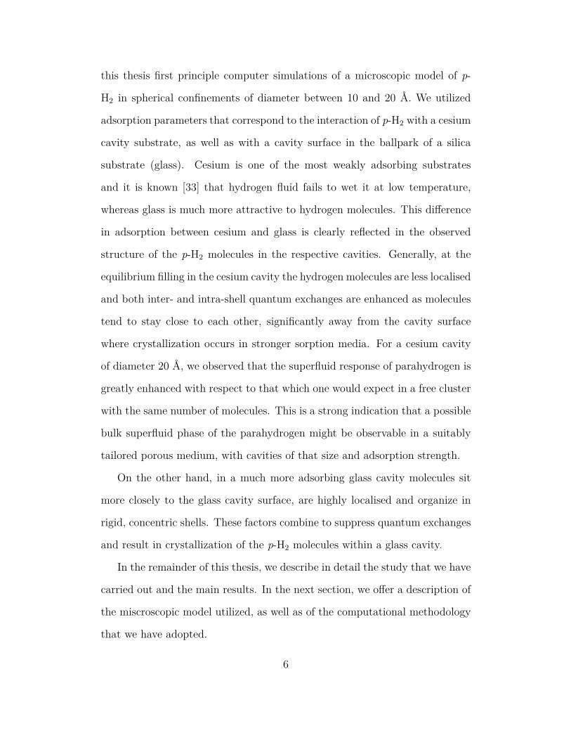
this thesis first principle computer simulations of a microscopic model of p-
H2 in spherical confinements of diameter between 10 and 20 Å. We utilized
adsorption parameters that correspond to the interaction of p-H2 with a cesium
cavity substrate, as well as with a cavity surface in the ballpark of a silica
substrate (glass). Cesium is one of the most weakly adsorbing substrates
and it is known [33] that hydrogen fluid fails to wet it at low temperature,
whereas glass is much more attractive to hydrogen molecules. This difference
in adsorption between cesium and glass is clearly reflected in the observed
structure of the p-H2 molecules in the respective cavities. Generally, at the
equilibrium filling in the cesium cavity the hydrogen molecules are less localised
and both inter- and intra-shell quantum exchanges are enhanced as molecules
tend to stay close to each other, significantly away from the cavity surface
where crystallization occurs in stronger sorption media. For a cesium cavity
of diameter 20 Å, we observed that the superfluid response of parahydrogen is
greatly enhanced with respect to that which one would expect in a free cluster
with the same number of molecules. This is a strong indication that a possible
bulk superfluid phase of the parahydrogen might be observable in a suitably
tailored porous medium, with cavities of that size and adsorption strength.
On the other hand, in a much more adsorbing glass cavity molecules sit
more closely to the glass cavity surface, are highly localised and organize in
rigid, concentric shells. These factors combine to suppress quantum exchanges
and result in crystallization of the p-H2 molecules within a glass cavity.
In the remainder of this thesis, we describe in detail the study that we have
carried out and the main results. In the next section, we offer a description of
the miscroscopic model utilized, as well as of the computational methodology
that we have adopted.
6

In Chapter 3 of this thesis, we present results of a study that is propaedeu-
tic to that of hydrogen in a cavity, and which we undertook before turning
our attention to the main problem of our interest. Specifically, the reliability
of a theoretical prediction on the behaviour of confined parahydrogen cru-
cially hinges on an accurate description of the interaction between hydrogen
molecules, over a wide range of pressures. This is because in confinement,
hydrogen molecules experience varying degrees of compaction throughout the
cavity, as the overall system is not homogeneous; thus, it is desirable to utilize
a pair potential capable of reproducing accurately the equation of state of p-H2
to high pressure. To this end, we considered a recently introduced pair poten-
tial, modified its repulsive core at short distance, and computed with it the
low temperature equation of state of solid parahydrogen. We found excellent
agreement of the experimentally measured equation of state for this system,
up to megabar pressure.
The results of our simulations of p-H2 in confinement as well as our ob-
servation of the enhancement of the superfluid response of these clusters in
cesium cavity are detailed in Chapter 4. This thesis concludes with a discus-
sion of the promising implications of our study for the realization of a stable
bulk superfluid phase of p-H2 in purposefully designed porous media.
7

Chapter 2
PHYSICAL MODEL AND
RESEARCH METHODOLOGY
In this chapter, we present details of the physical model and computa-
tional approach adopted in our study of the superfluidity of para-hydrogen in
nanoscale confinement.
2.A The Many-body Hamiltonian
Our system of interest consists of N p-H2 molecules, represented as point
particles of spin zero, enclosed in a spherical cavity of radius R, and is described
by the following quantum-mechanical many-body Hamiltonian:
H = −λ∑
i
∇2i +
∑
i<j
v(rij) +∑
i
V (ri). (2.1)
Here, the ri are positions of all p-H2 molecules, measured with respect to
the centre of the cavity (made the origin), rij ≡ |ri − rj| is the distance
8

between two p-H2 molecules; λ= ~2
2m=12.031 KÅ2, m being the mass of a p-H2
molecule; v describes the interaction between any pair of p-H2 molecules, while
V describes the interaction of a p-H2 molecule with the cavity. For v, which
we regard as spherically symmetric, we use a modification of the well-known
pair potential of Silvera and Goldman [34], which has been shown to afford an
accurate reproduction of the experimental equation of state of solid p-H2 up to
megabar pressure [35]. Such accuracy for the equation of state is crucial for an
inhomogeneous system like the one we are dealing with, as hydrogen molecules
at different parts of the cavity certainly experience varying pressures, which
could be very high close to the cavity surface; we discuss this in greater detail
in Chapter 3. For V , assumed to be a function of only the distance of a
molecule from the centre of the cavity, we take the following model potential
[36]:
V (r) = 2D
b9F (x)(1 − x2)9
− 6b3
(1 − x2)3
, (2.2)
where x ≡ r/R, F (x) = 5 + 45x2 + 63x4 + 15x6, b ≡ (a/R), r is the distance
of a p-H2 molecule from the centre of the cavity, R is the fixed radius of the
cavity, and a, D are two parameters that are adjusted to reproduce, as closely
as allowed by such a relatively crude model, a specific particle-substrate in-
teraction. Eq. (2.2) is the generalization to the case of a spherical cavity
of the so called “3-9” potential, which describes the interaction of a particle
with an infinite, planar substrate [36]. It is derived by considering the cavity
enclosure as a uniform outward extension of the substrate, extending from the
surface of the spherical cavity (enclosing the p-H2 molecules) to infinity. An
infinitesimal element of volume of the medium is then considered to interact
with a molecule in the enclosed cavity via Lennard-Jones potential, also de-
9

scribed in Chapter 3. The three dimensional integral of such interactions with
the particle (a p-H2 molecule) located at a position ri relative to the cavity’s
centre, results in V (ri) evaluated at ri = |ri| as presented in Eq. (2.2). The
parameter D in Eq. (2.2) has the dimensions of an energy, and is essentially
the depth of the attractive well of the potential experienced by the particle in
the neighbourhood of the substrate, whereas a is a characteristic length, cor-
responding approximately to the distance of closest approach to the substrate,
where the molecule begins to experience a strong repulsion.
It is worthwhile to clarify at this point that the model of the system that
we employ here does contain some simplifications, primarily the assumption
that the interaction between hydrogen molecules can be sufficiently accurately
represented by a spherically symmetric pair potential, as well as the fact that
a cavity is regarded as perfectly spherical and smooth. Even though one might
expect significant alterations to the interaction between two p-H2 molecules
inside a nanoscale cavity, the weakness of the substrate seems to justify the
continued use of a central pair potential as if the molecules interacted in vac-
uum. This is based on the expected minimum distance from the surface (over
3 Å) at which molecules will be sitting, as confirmed by our simulation re-
sults [37]. On the whole, regardless of its simplicity, such a model allows us
to address the physical question we are exploring in this thesis, which is the
effect of confinement on the superfluid response of p-H2. Actually, equivalent
or even simpler models (e.g., cavities with hard walls) have been adopted to
investigate structure of 4He and classical fluids in confinement [38, 39].
We have thus carried out a theoretical investigation of the low temperature
(T → 0) physical properties of the system described by Eqs. (2.1) and (2.2),
by means of first principle computer simulations. We specifically utilized the
10

Worm Algorithm in the continuous space path integral representation. This
well-established computational methodology enables one to compute thermo-
dynamic properties of Bose systems at finite temperature, directly from the
microscopic Hamiltonian, and it gives direct access to the energetic, structural
and superfluid properties of the confined p-H2 fluid, in practice with no uncon-
trolled approximations. It is therefore a well suited computational approach
to address directly the physical issues of interest here.
2.B The Continuous-space Worm Algorithm
The Path Integral Monte Carlo (PIMC) technique is the most reliable com-
putational method for studying superfluidity and Bose-Einstein condensation,
as well as the connection between the two phenomena [40]. Our calculations
exclusively utilize Path Integral Monte Carlo (PIMC) simulations based on
the Continuous Space Worm Algorithm [41, 42]. The PIMC approach involves
implementing the Feynman’s Path Integral [43] formalism through a suitable
Monte Carlo strategy. The PIMC scheme is accurate and has no adjustable
parameter, taking the microscopic Hamiltonian as its only input. It also does
not have any inherent bias, since no a priori assumption, e.g., a trial wave
function, is needed. The methodology is numerically exact for Bose systems.
For Fermi systems, not considered in this work, it is only approximate.
2.B.1 Thermal Averages and Path Integration
The thermal average of a physical observable, for an N -particle system
described by Eq. (2.1) at temperature T , represented by an operator O, is
11

given by
〈O〉 =Tr (Oρ)
Tr ρ=∫
dR O(R)ρ(R, R, β)∫
dR ρ(R, R, β)(2.3)
where R ≡ r1 r2 . . . rN , i.e, the positions of all the N particles in the N -
particle configuration and β = 1/(kBT ). Henceforth, we shall set kB = 1. The
many-body density matrix, ρ(R, R, β), is given by
ρ(R, R, β) = 〈R|e−βH |R〉 (2.4)
with H being the quantum-mechanical many-body Hamiltonian of Eq. (2.1)
while the partition function is given by
Z =∫
dR ρ(R, R, β) .
The many-body density matrix is not usually known and Eq. (2.3) is
evaluated through the path integration procedure prescribed by R. P. Feynman
in 1948. Accordingly, the partition function,
Z ∝∫
DR(u) exp −S[R(u)] . (2.5)
The integration in Eq. (2.5) is performed over all possible continuous, β-
periodic N -particle configuration paths R(u).
S[R(u)] is the Euclidean action expressed as
S[R(u)] =∫ β
0du
N∑
i=1
m
2~2
(
dri
du
)2
+ V(R(u))
, (2.6)
having defined u~ as the “imaginary time”. V =∑
i<j v(rij)+∑
i V (ri) as given
12

in Eq. (2.1). The Euclidean action is related to path balance between kinetic
(path curvature) and potential energy, which depends on interactions, along
the various paths. Generally, smooth, straight paths have higher probability
while paths of high potential energy have lower probability.
2.B.2 Path Integral Monte Carlo and Quantum Statis-
tics
The evaluation of the many-body density matrix, Eq. (2.4), the parti-
tion function, (2.5), and the thermal average, (2.1), is most suitably achieved
through a well implemented Monte Carlo strategy. This involves employing the
Metropolis Algorithm [44] to sample many-particle paths R(u) through config-
uration space, based on a probability distribution proportional to exp[−S(R(u))].
Thermal expectation values, such as (2.1), are then calculated as statistical av-
erages of the physical observable of interest along paths.
In the continuum, the action integral must be discretized. This leads in-
evitably to a time-step error that can however be made arbitrarily small. The
discretization procedure is such that in place of the continuous many-particle
path R(u), one considers a discrete path R(u) ≡ R0, R1, . . . , RM−1 for a
finite number of time slices M . The β-periodicity of the paths requires that
RM = PR0, where P denotes permutations of particle labels. Any choice of a
finite M defines a corresponding time step, τ , such that Mτ = β. The simplest
approximate action (due to path discretization) is given by
S[R(u)] ≈N∑
i
M−1∑
l=0
m(ril − ril+1)2
2τ~2+ τ
M−1∑
l=0
V(Rl) . (2.7)
13

(Indeed, were V = 0 (no interaction between particles), any discretized form
becomes exact as M → ∞). The probability with which a discrete path R(u)
is sampled is then given by
P ∝ exp −S[R(u)]
=N∏
i=1
M−1∏
l=0
ρ(ril, ril+1, τ) ×M−1∏
l=0
e−U(Rl,τ) ,(2.8)
where
ρ(r, r′, τ) =(
2π~2τ/m)−d/2
exp
[
−m(r − r′)2
2~2τ
]
(d is the dimensionality of the configuration space)
(2.9)
is the density matrix of a free particle, and in the simplest approximation, Eq.
(2.7),
U(R, τ) = τV(R) . (2.10)
U(R, τ) will change in other approximations of the action, S, so that the
discrete action becomes exact in the limit M → ∞.
Quantum statistics, i.e, particle indistinguishability, is effected in the above
formalism by allowing R(β=Mτ) = PR(0), the permutation P implying that,
while actual positions occupied by particles in R(β) and R(0) are the same,
particles are allowed to trade place. This is a crucial ingredient, in Bose
systems, to allow for the capturing of the physics of the system, such as su-
perfluidity and Bose-Einstein condensation, underlain by quantum exchanges
and particle indistinguishability [45].
Finally, the thermal expectation of a physical observable O, given by Eq.
14

(2.3), is then evaluated as
〈O〉 ∼∑
paths ηPO(Rpath)∑
paths ηP(2.11)
where P is the parity of the permutation associated with particle relabelling
(exchange), O(Rpath) is the average value of O along a path and η = +1 for
Bose , -1 for Fermi statistics.
The direct averaging over paths as expressed in Eq. (2.11) becomes ex-
ponentially intractable with increasing N for Fermi systems as the sum over
paths comprises “an alternating series of terms of opposite signs”, which very
nearly cancel each other out, as is well communicated in Ref. [46]. This results
in a very low “signal-to-noise” ratio, rendering the calculation not feasible in
practice at low temperature.
For Bose systems, on the other hand, η = +1, and therefore no such prob-
lem arises. Because in this work we are only concerned with Bose systems, we
shall make no further mention of the above difficulty, referred in the literature
as “sign problem of quantum Monte Carlo”.
2.B.3 Thermal Wavelength and Particle Permutations
Although in principle permutations of identical particles must be included,
one can come up with a simple physical criteria to determine their importance
in a given system at temperature T .
The characteristic “size” of a single particle path is measured by the ther-
mal wavelength
λT =~√mT
15


world lines of individual particles in pairs and attempting to reconnect them
together to achieve exchange cycles, while remaining in the diagonal sector of
the configuration space. However, in the presence of any realistic interaction
potential, typically possessing a repulsive and hard core, any such sampling
of permutations is bound to have high likelihood of rejection and therefore
becomes inefficient. Rejection occurs because the constructed trial path will
almost always bring two particles within near vicinity of each other, i.e, the
trial configuration will have high potential energy. In practice, efforts required
to sample macroscopic permutation cycles scales exponentially with the sys-
tem size. This challenge limits the number of particles for which the low
temperature thermodynamics of a system can be effectively studied, making
accurate extrapolation of results to the thermodynamic limit highly problem-
atic, using the conventional PIMC implementation. The conventional PIMC
implementation also does not allow for the simultaneous evaluation of diagonal
and off-diagonal correlations, as its configuration space is locked in a canonical
ensemble.
2.B.5 Effective Permutation Sampling: The Worm Al-
gorithm
The Worm Algorithm completely resolves the issues mentioned above. A
fundamental feature of the continuous-space worm algorithm is that it func-
tions in an extended configurational space, including both closed world line
configurations, referred to as the Z-sector, as well as configurations having
one open world line (worm), known as the G-sector. A schematic view of the
G-sector of the configuration space of the worm algorithm is seen in Fig. (2.2)
17

Green function reduces to the one-particle density matrix, n(r2, r1), from which
the momentum distribution is computed [50] directly in the continuous-space
Worm Algorithm.
The Worm Algorithm accurately calculates various thermodynamic quan-
tities of interest for large Bose systems in easily accessible computation time.
These quantities include the energetics, structure, superfluid density, conden-
sate fraction, one-body density matrix and momentum distribution. Another
elegant feature of the Worm Algorithm is that it can be implemented in ei-
ther a canonical or a grand-canonical ensemble (resulting from fluctuations of
particle number through annihilation and creation of worms).
In our current application of the Worm Algorithm, the Z-sector configura-
tions have a fixed number N of particles, while configurations in the G-sector
are constrained to having N − 1 particle world lines and a single worm.
Path Sampling In The Worm Algorithm
The Worm Algorithm automatically affords extensive sampling of intri-
cate and non-trivial permutation cycles in both the Z- and G- sectors, while
maintaining ergodicity regardless of the strongly repulsive core of microscopic
interactions. This is readily achieved by its use of ergodic local path updates,
in complementary pairs, that efficiently sample paths in its extended configu-
ration space. For details, the reader is referred to Refs. [41, 42].
2.B.6 Thermodynamic Estimators
Having utilized the Worm Algorithm to obtain space-time configurations,
of any quantum-mechanical system of interest, which are drawn from the ap-
19

propriate probability distribution (Eq. (2.8)), one becomes fully equipped to
accurately compute the thermodynamic properties of the system, using ap-
propriate thermodynamic estimators. For our study of superfluid hydrogen
in nanoscale confinement, we computed the equilibrium total energy per p-
H2 molecule, e(N), superfluid fraction, ρS(T ), radial density profile, ρ(r) and
the momentum distribution, n(k). The total energy per particle, useful for
calculating the equation of state of the system, is obtained by summing its
kinetic, 〈K〉 and potential, 〈V〉, parts. These are calculated as described in
Refs. [47, 51] as follows:
〈K〉 ≈ 32τ
− 14λτ 2
⟨
(rl − rl+1)2⟩
+λτ 2
9
⟨
(
∇V(R2l))2⟩
, (2.13)
where 〈· · · 〉 indicates the statistical average of the enclosed quantity, (rl − rl+1)2
is the square of the spatial separation of adjacent beads along a world line, while
the gradient of the potential energy V is obtained with respect to the coordi-
nate of one of the particles at an even time slice. For the potential energy per
particle, the expression is
〈V〉 ≈ 1N
〈V(R2l−1)〉 . (2.14)
Eqs. (2.13) and (2.14) both approach the exact results in the limit M → ∞,
τ → 0.
The superfluid fraction (ρS(T )), i.e., the fraction of a finite system that
uncouples from a rotation that is induced externally, is obtained in the PIMC
formalism as
ρS(T ) =4m2T
~2Ic
〈A2〉 , (2.15)
20

where A is the projection of the total area covered by the many-particle paths
unto a perpendicular plane to one of the three symmetric rotation axes, Ic is
the classical moment of inertia of the finite system (e.g p-H2 cluster) and Eq.
(2.15) is known as the area estimator [52].
As explained in Ref. [50], the momentum distribution is obtained from the
one body density matrix n(r, r′) which is the τ → 0 limit of the Matsubara
Green function, G(r, r′). For a system that is traslationally invariant, n(r, r′) ≡
n(r − r′), and n(k) is given by the inverse transform
n(k) =∫
d3r n(r)e−ık·r , (2.16)
which for a system with spherically symmetric momentum distribution, i.e.,
n(k) ≡ n(k), becomes
n(k) =4π
k
∫
∞
0dr r sin kr n(r) , (2.17)
having fixed the value of the one-body density matrix to unity at r = 0, hence
the normalization1
(2π)3
∫
d3k n(k) = 1. (2.18)
One then obtain the one body density matrix (OBDM) as described in Ref.
[48].
We also estimate the standard error on our calculated expectation values.
This is necessary as the expectation values are obtained as statistical averages
using finite number (M) of configurations (X) and the mean of a physical
observable over sample configurations will neccessary deviate from, and flunc-
tuate around, the true mean of the normal distribution that is reached in the
21

limit M → ∞. However, a straightforward estimate of the standard error on
the mean using
〈O〉σ =
√
√
√
√
∑
M
k=1(O(Xk) − 〈O〉)2
M(M − 1), (2.19)
would underestimate the error, since the elements of our Markov chain are
not completely independent and there exist an autocorrelation between the
various O(Xk) given by [53]
〈OkOk+1〉 − 〈Ok〉2
〈O2k〉 − 〈Ok〉2 . (2.20)
A reliable estimate of the standard error is obtained by reducing the autocor-
relation between the quantities over which the average is sought. One way
to do this would be to bin the entire M configurations into smaller configu-
rations, average over each of the smaller configurations (thereby obtaining a
set of averages that are less correlated than the initial set of averages over the
original configurations set), and then finding the standard error on these new
set of averages. We carry out a more rigorous estimation of the standard error
using the blocking/bunching method (See Refs. [49, 54]).
22

Chapter 3
PAIR POTENTIALS AND
EQUATION OF STATE OF
SOLID PARA-HYDROGEN TO
MEGABAR PRESSURE
An accurate T = 0 Path Integral Monte Carlo (PIMC) study of the system
which we consider in this thesis, i.e., para-hydrogen clusters confined in spher-
ical cavities, requires that one be able to reliably predict the equation of state
of p-H2 at non-trivial densities corresponding to very high pressures in the Gpa
range. This is because the system is not homogeneous as in the hexagonally
packed bulk structure, but the pressure exerted on a p-H2 molecule may vary
significantly throughout the cavity. Consequently, we carried out a detailed
study of the accuracy of three different pair potentials in predicting the equa-
tion of state of solid p-H2 to megabar pressure, covering the entire pressure
range for which there is experimental data.
23

We compute by means of Quantum Monte Carlo simulations the equation
of state of bulk solid p-H2 extrapolated to zero temperature, up to a pressure
of ∼2 Mbar. A comparison is made of the equation of state obtained by us-
ing the Silvera-Goldman (SG) and Buck [55] potentials, as well as a potential
recently proposed by Moraldi [56], modified at short distances to include a
repulsive core, missing in the originally proposed one. The Moraldi pair po-
tential yields an equation of state in excellent agreement with experiment at
megabar pressures, owing to its softer core, and is at least as accurate as the
Buck at saturated vapor pressure.1 This provides, to non-trivial pressures, a
highly dependable description of the interaction between hydrogen molecules
in a wide variety of configurations.
3.A Introduction
Hydrogen is known to be the simplest and most abundant element in the
universe. Achieving predictive knowledge of its equation of state in a wide
range of thermodynamic conditions has always been a worthwhile theoretical
goal, owing to its relevance in a broad variety of physical systems, usually with
possible technological applications [57, 58, 59], and also because it provides a
cogent assessment of the most advanced computational many-body techniques.
The equation of state (EOS) of hydrogen, in essentially all phases of in-
terest, is a fully quantum-mechanical problem. This is due to the fact the
thermal wavelength of hydrogen is of the order of its mean inter-particle dis-
tance, causing the probability cloud (due to zero point motion) of individual
1A version of this chapter has been published as:Tokunbo Omiyinka and Massimo Boninsegni. Physical Review B 88, 024112 (2013).
24

molecules to significantly overlap with their neighbour’s. Theoretical calcula-
tions broadly fall into two different categories; in ab initio studies, the mathe-
matical model explicitly takes into account the ionic and electronic degrees of
freedom, and their interaction via electrostatic Coulomb potential. Calcula-
tions are carried out within the framework of density functional theory (DFT)
[60, 61, 62, 63, 64, 65] or Quantum Monte Carlo (QMC) [66, 67, 68, 69, 70, 71].
On the other hand, in molecular condensed phases, one often adopts the
Born-Oppenheimer approximation, allowing one to regard individual hydro-
gen molecules as elementary particles, thus ignoring the electronic degrees of
freedom. This approximation is mostly justified on the ground that the energy
change pertaining to the first electronic excited state is of the order of 1 eV
or ∼11588 K, which is order of magnitudes greater than the temperatures at
which our studies are made (≤ 4 K), allowing us to consider the p-H2 molecules
as being effectively in their electronic ground state. Thus, one is able to de-
scribe the interaction between the molecules by means of a static potential,
the simplest choice being that of a central pair potential.
In Fig. 3.1, we show the simplest example of a central pair potential, the
Lennard-Jones potential, given by
V (r) = 4ǫ
[
(
σ
r
)12
−(
σ
r
)6]
. (3.1)
It shows the strong repulsion at short distances, characteristic of all micro-
scopic pair potentials, due to Pauli exclusion principle preventing electrons
of different molecules from spatially overlapping. Also evident are the weak
attraction at long intermolecular distances (r ≫ σ) owing to mutually induced
electric dipoles, as well as a maximum well depth ǫ ∼ 30 K and core σ ∼ 3 Å,
25

0
2
4
6
1.2 1.6 2 2.4
V(∈
)
r(σ)
V(r)
Figure 3.1: Lennard-Jones Potential
[V (σ) = 0]. More elaborate potentials are constructed in an attempt to pro-
vide better description of both the repulsive core and attractive tail. Notable
examples for hydrogen are the Silvera-Goldman and Buck pair potentials.
Obviously, an approach based on a pair potential only dependent on the
spatial separation between two molecules cannot describe any process involv-
ing electronic transfer, nor the energy contribution of interactions involving,
say, triplets of molecules, nor any effect arising from the non-spherical fea-
tures of the intermolecular interaction; the importance of all of these physical
mechanisms generally increases with the thermodynamic pressure of the con-
densed phase under study. There are, however, distinct advantages to the
use of static pairwise potentials, mainly, that it is typically computationally
much faster and conceptually simpler than ab initio methods. Furthermore,
if pair potentials are used, thermodynamic properties of molecular hydrogen
26

in condensed phase, and certainly in confinement, can be typically computed
essentially without any uncontrolled approximation, e.g., by means of QMC
simulations. Thus, it is desirable to develop pair potentials that afford reason-
ably accurate, quantitative description of the condensed phase of hydrogen in
broad ranges of thermodynamic conditions. The Silvera-Goldman model pair
potential is arguably the most commonly adopted, and has been shown [72]
to afford a quantitative description of the low temperature equilibrium solid
phase of p-H2, whose superfluidity in nanoscale confinement we set out to ex-
amine. Another well known pair potential is the Buck [73, 74], which is very
similar to the Silvera-Goldman, albeit with a slightly deeper attractive well.
Both potentials yield an equation of state in reasonable agreement with ex-
periment at moderate pressure (.25 kPa). At higher pressure, however, they
become increasingly inaccurate, leading to an overestimation of the pressure
due to the excessive “stiffness” of their repulsive core at short intermolecular
separation (below ∼2.8 Å). This challenge is also present in the theoretical cal-
culation of the equation of state of condensed helium at high pressure, based
on pair potentials; in that context it is known that including three-body terms
gives better agreement with the experimental equation of state, the overall
effect being that of softening the repulsive core of the pairwise interaction
[75, 76, 77].
Still, given the significant computational overhead involved in the inclusion
of three-body terms, there remains the question of whether a modified effective
pair potential could offer more satisfactory agreement of theory with experi-
ment at high (e.g., megabar) pressure. To this aim Moraldi recently proposed
a modified effective pair potential, with a softened repulsive core, designed to
afford greater agreement between experiment and the theoretically predicted
27

values of the pressure as a function of the density in the low temperature limit
(T → 0). Results of perturbative calculations carried out in Ref. [56] show
remarkable agreement with experimental data of the pressure computed with
the new pair potential, in an extended range of density (up to 0.24 Å−3, which
corresponds to a pressure in the megabar range).
In this work, the T = 0 equation of state of solid p-H2 is computed by
means of first principle QMC simulations in a wider density range with re-
spect to Ref. [56], namely, up to a density of 0.273 Å−3, for a model of
condensed p-H2 based on three different pair potentials; our slightly modified
version of the Moraldi potential (as shown in Fig. 3.2), the Silvera-Goldman,
and the Buck. We provided a numerically accurate, non-perturbative check
of the pressure computed in Ref. [56], and we offered a cogent comparison
of the performance of the three potentials. We also compute the total and
kinetic energy per molecule; the latter is experimentally measurable by means
of neutron scattering, and is particularly sensitive to the detailed features of
the repulsive core of the interaction [75].
We find that the recently proposed pair potential does indeed yield pressure
estimates in much better agreement with experiment than the Silvera-Goldman
and Buck potential, especially above 0.14 Å−3. In fact, the agreement between
the values of the pressure computed with the modified Moraldi potential and
the ones measured experimentally remains excellent up to ∼180 GPa, the
highest pressure for which experimental data are available for solid H2. At the
equilibrium density, i.e., zero pressure at T = 0, the Moraldi potential yields
energy estimates comparable to those of the Silvera-Goldman. Kinetic energy
estimates at high density computed with the Moraldi potential are significantly
lower than those furnished by the Silvera-Goldman and Buck potentials, a fact
28
ascribable to the softer repulsive core of the Moraldi pair interaction. An ex-
perimental measurement of the kinetic energy will therefore provide additional
important insights on whether the Moraldi potential not only yields an equa-
tion of state in quantitatively close agreement with experiment, but also affords
a generally more accurate, quantitatively physical description of the system
than the Silvera-Goldman or Buck model interactions.
We continue this chapter by presenting the particular microscopic model
we adopt therein. We also illustrate the pair potentials we utilized, briefly
highlighting the basic methodology underlying the calculation and offering
relevant computational details in Sec. 3.C. In Sec. 3.D a thorough illustration
of the results obtained in this work is provided. We finally provide a general
discussion and conclusion to this chapter in Sec. 3.E.
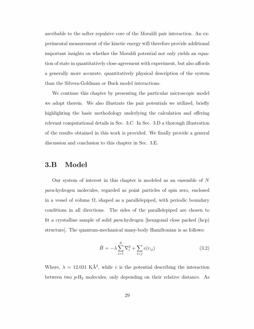
3.B Model
Our system of interest in this chapter is modeled as an ensemble of N
para-hydrogen molecules, regarded as point particles of spin zero, enclosed
in a vessel of volume Ω, shaped as a parallelepiped, with periodic boundary
conditions in all directions. The sides of the parallelepiped are chosen to
fit a crystalline sample of solid para-hydrogen [hexagonal close packed (hcp)
structure]. The quantum-mechanical many-body Hamiltonian is as follows:
H = −λN∑
i=1
∇2i +
∑
i<j
v(rij) (3.2)
Where, λ = 12.031 KÅ2, while v is the potential describing the interaction
between two p-H2 molecules, only depending on their relative distance. As
29

we do make comparison between results from different pair-potentials in this
work, we also provide here some basic details of all potentials used. The
Silvera-Goldman (VSG) and Buck (VB) have the form
V (r) = Vrep(r) − Vatt(r)fC(r), (3.3)
where Vrep(r) describes the repulsion of two molecules at short distances, aris-
ing mainly from the Pauli exclusion principle, preventing the electronic clouds
of different molecules from spatially overlapping, whereas Vatt(r) represents
the long-range van der Waals attraction of mutually induced molecular elec-
tric dipoles. The purpose of the function fC(r) is to remove the divergence of
Vatt(r) as r → 0. For the Silvera-Goldman potential, Vrep is given by
Vrep(r) = e−α−βr−λr2
, (3.4)
while Vatt is given by
Vatt =C1
r6+
C2
r8− C3
r9+
C4
r10. (3.5)
Finally, fC(r) is given by
fC(r) =
e−( r0
r−1)2
if r < r0,
1 otherwise. (3.6)
The value of the constant parameters in the Silvera-Goldman expression are
provided in Ref. [34]. In Vatt, the term proportional to r−9 is the Axilrod-
Teller estimate of the effective contribution of three-body interactions to the
30

potential, expected to be increasingly significant at high pressure and very low
temperature (T → 0). The expression for the Buck potential is similar to that
of Silvera-Goldman, save the absence of the three-body term and the different
values of its corresponding constants. As proposed in Ref. [56], the Moraldi
potential is expressed as follows:
VM(r) = Vrep(r)frep(r) − Vatt(r)fC(r), (3.7)
where the functions Vrep, Vatt, and fC are the same as in the Silvera-Goldman
potential; whereas frep, being of the same form as fC , softens the repulsion at
short distances contained in Vrep. It is given by
frep =
exp(
−a(
r0
r− 1
)n)
if r < r0,
1 otherwise. (3.8)
where a = 0.95, r0 = 5.2 a.u (1 a.u = 0.529 Å), and n = 1.5. The potential
VM(r), as shown in Ref. [56], displays a much slower growth as r → 0 than
the Silvera-Goldman. In fact, the function VM(r) stops growing altogether
at r ∼ r0 (see Fig. 3.2 below). This unphysical feature of VM(r) is of little
consequences in calculations at low density, but must be corrected in order to
prevent particles from “tunnelling” across the potential barrier and piling on
top of one another, something we observed in computer simulations making
use of VM(r) at densities for which the intermolecular distance is .2 Å. Thus,
in this work we made use of the modified potential U(r), defined as follows:
U(r) = VM(r)Θ(r − d) + VrepΘ(d − r), (3.9)
31

0
1
2
3
4
0.5 1.5 2.5 3.5
V (
10 K
)4
r (A)o
OriginalModified
Figure 3.2: The Moraldi pair potential VM(r) as proposed in Ref. [56](solid line) and the modified one U(r) used in the present work (dashedline) [35]
.
where d = 4 a.u (i.e. 2.1167 Å), Θ(x) is the Heaviside function, and Vrep(r) has
the same form of Vrep, but the two parameters (usually referred to as α and β)
upon which it depends are adjusted to match VM(r) and its first derivative at
r = d. This modified potential, utilized in our simulations, is shown alongside
VM(r) in Fig. 3.2. It lacks the unphysical feature of VM(r) at short distances
discussed above; indeed, it increases monotonically as r → 0.
3.C Calculation
The T = 0 (ground state) equation of state of solid para-hydrogen, mod-
elled by the many-body Hamiltonian (3.2) with the three different potentials
32

VSG, VB and U described above, was computed by means of numerical QMC
simulations based on the Continuous-Space Worm Algorithm. Specifically,
we computed the pressure P as a function of the density ρ, in the interval
0.0763 Å−3 ≤ ρ ≤ 0.273 Å−3, for a finite system comprising N = 216 molecules.
In order to provide ground state estimates, we perform simulations at different
low temperatures and extrapolate the results to T = 0. We generally find that
results obtained at T = 4 K are indistinguishable from the extrapolated ones,
within our quoted statistical uncertainties. We employ the standard virial es-
timator [78] for pressure, and estimate the contribution from particles lying
outside the main simulation cell by radially integrating the quantity r(dV/dr),
approximating the pair correlation function g(r) to 1 (we do the same for the
potential energy) [79].
Density Time step Energy Pressure0.076 39 × 10−4 1.40 × 10³ 5.75 × 10⁴
0.076 20 × 10−4 1.50 × 10³ 5.79 × 10⁴
0.076 10 × 10−4 1.53 × 10³ 5.92 × 10⁴
0.076 5.0 × 10⁻⁴ 1.53 × 10³ 5.92 × 10⁴
Table 3.1: Time step extrapolation (τ → 0) for Pressure (in bars)and Energy in (K) calculated at 0.076 Å−3) in the T → 0 limit, usingSilvera-Goldman potential. Combined statistical and systematic errorsaffecting our QMC simulations are estimated to be of the order of 0.1%or less of the quoted values.
We obtain our QMC results, as presented herein, with a time step τ =
5×10⁻⁴ K−1. Indeed, we observed that the estimates yielded by such a choice
of time step coincide with those extrapolated to τ = 0, within statistical uncer-
tainties, as illustrated in Table 3.1. It is worth emphasizing that, in principle,
para-hydrogen molecules must be regarded as indistinguishable particles of spin
33

zero, and thus obeying Bose statistics. The Worm Algorithm explicitly allows
for permutation of identical particles, and quantum-mechanical exchanges can
be important in p-H2, in specific situations. They are in fact known to un-
derlie superfluidity at low temperature in small clusters (< 30 molecules) [80],
and their effect is measurable in the momentum distribution of liquid para-
hydrogen near melting [81]. However, in the solid phase, in the range of density
explored here, exchanges are practically absent, i.e., particles can be regarded
for practical purposes as distinguishable.
3.D Results
While our work in this chapter is mainly aimed at the equation of state
of solid p-H2 at relatively high (megabar) pressure, we start the discussion of
our results by illustrating the results of QMC simulations at the saturation
density ρ = 0.0261 Å−3. Specifically, we compare the pressure and energy es-
timates yielded by the Moraldi potential (modified as explained above), which
was not purposefully designed to describe the low-density equilibrium phase,
to those yielded by the Silvera-Goldman and Buck potentials, as well as to
experimental data. We make such a comparison in order to ascertain whether
the softening of the Silvera-Goldman repulsive core, which is at the basis of
the Moraldi potential, might worsen the agreement with experiment at low
density while possibly improving it in the megabar pressure range. Table 3.2
shows numerical estimates of the ground state energy per molecule for solid
para-hydrogen at saturation density. The estimates here, obtained by extrap-
olating all the way down to T = 0 results obtained in the range 1 K ≤ T ≤ 4
K, are in agreement with those given in Ref. [72] using ground state diffusion
34

This work Ref. [72]Moraldi -88.5(2)
Silvera-Goldman -88.1(1) -87.90(2)Buck -93.8(1) -93.87(2)
Table 3.2: Ground state energy per molecule (in K) for solid parahy-drogen in the hcp phase at the saturation density ρ = 0.0261 Å−3,computed in this work and in Ref. [72] for various intermolecular po-tentials. Statistical errors, in parentheses, are on the last digit.
Monte Carlo (DMC) simulations. Experimentally, the ground state energy per
molecule has been inferred by various methods, and the agreement between
the various predictions [82, 83, 84, 85] is not perfect; quoted values range from
-89.9 K of Ref. [84] to -93.5 K of Refs. [83] and [85]. It is obvious from
the data reported in Table 3.2 that the Moraldi potential affords an accuracy
comparable to that of the other two potentials.
We make a comparison in Fig. 3.3 of our computed values of the pressure
(with the three pair-potentials) for hcp para-hydrogen in the T → 0 limit, in
a density range up to 0.273 Å−3, which corresponds to a pressure of about 1.8
Mbar. Also included for comparison is a fit to the most recent [86] compilation
of experimental (x-ray) measurements [87, 88, 89] of the equation of state
obtained with the Vinet equation of state [90],
P =3K(1 − d)
d2exp
[32
(K ′
− 1)(1 − d)]
, (3.10)
where d ≡ (ρ/ρ)1/3, with parameters K = 0.20(1) GPa and K ′ = 6.84(7).
We also report the computed values of the pressure in Table 3.3.
The agreement between the experimental values of the pressure and those
obtained by simulation using the Moraldi potential is excellent, considering the
35

0
100
200
300
400
0.08 0.12 0.16 0.20 0.24 0.28
Pre
ssure
(G
Pa)
Density (A )o-3
BuckSGMoraldiExperiment
Figure 3.3: Equation of state of solid parahydrogen at T=0, computedby Quantum Monte Carlo simulations using the Silvera-Goldman (di-amonds), Buck (circles) and Moraldi (boxes) pair potentials. Dashedline represents a fit to experimental data from Ref. [86] obtained withthe Vinet equation of state (see text). Combined statistical and sys-tematic errors affecting our computed pressures are at the most of theorder of 0.1% of the pressure.
relatively simple form of the pair potential itself. At the highest compaction
examined here, i.e., 0.273 Å−3, the Silvera-Goldman potential overestimate
the pressure by over a factor of 2. The Buck potential does only slightly
better than the Silvera-Goldman. The lower values of pressure yielded by
the Moraldi potential are a direct consequence of its softer repulsive core. It
is noteworthy that the values in Table 3.3 agree quantitatively with those
obtained by Moraldi in Ref. [56], using a perturbative calculation. Perhaps
a more significant fact is the excellent agreement with experiment obtained
using the modified Moraldi potential even above 110 GPa, i.e., a compression
at which solid hydrogen undergoes an orientational phase transition [91]. One
36

Density Moraldi Buck SG0.076 5.11 × 10⁴ 6.09 × 10⁴ 5.92 × 10⁴
0.098 1.17 × 10⁵ 1.54 × 10⁵ 1.52 × 10⁵
0.129 2.61 × 10⁵ 3.87 × 10⁵ 3.93 × 10⁵
0.174 5.93 × 10⁵ 9.74 × 10⁵ 1.04 × 10⁶
0.243 1.34 × 10⁶ 2.47 × 10⁶ 2.79 × 10⁶
0.273 1.80 × 10⁶ 3.40 × 10⁶ 3.94 × 10⁶
Table 3.3: Pressure (in bars) calculated for different densities (in Å−3)in the T → 0 limit, using Buck, Silvera-Goldman and Moraldi poten-tials. Combined statistical and systematic errors affecting our QMCsimulations are estimated to be of the order of 0.1% or less of thequoted values.
would anticipate that the approximation of a spherically symmetric potential,
for the interaction between two p-H2 molecules, would break down quickly as
the system assumes the orientationally ordered phase.
The fact that the Moraldi potential is not as stiff as the Silvera-Goldman or
Buck potentials at short distances is also reflected on the predicted structural
properties of the crystal. Specifically, the local environment experienced by a
single molecule is captured by the static structure factor, which of course can
be probed by x-ray diffraction. Its Fourier inverse, the pair correlation function
g(r), is easily accessible by simulation. Results for two different densities are
shown in Fig. 3.4, where the pair correlation functions computed for the Buck
and Moraldi potentials are juxtaposed. The SG and Buck potentials yield
similar results for this quantity [the main peak of the g(r) being ∼10% higher
with the SG potential, at the higher density]. While at the lower density,
which corresponds to a pressure around 5 kbar, the pair correlation functions
yielded by the two potentials are comparable, at the higher density (which
corresponds to a pressure close to 1 Mbar), there is a clear difference between
37

0
1
2
3
4
5
2 3 4 5 6
r(A)
BuckMoraldi
“ = 0.0763 A
o
o -3
ρ = 0.0763 Å-3
r (Å)2 3 4 5 6
2
4
0
BuckMoraldi
1 2 3 4
r (A)
BuckMoraldi
“ = 0.2428 A
o
o -3
BuckMoraldi
ρ = 0.2428 Å-3
r (Å)2 4 6
Figure 3.4: Pair correlation function g(r) for hcp para-hydrogen atT=4 K, computed by simulation at the two densities ρ=0.0763 Å−3
and ρ=0.2428 Å−3, with the Moraldi and Buck potentials. The resultsfor the Silvera-Goldman potential are similar to those for the Buck.
the two results. In particular, the pair correlation function computed with
the Buck potential has considerably higher peaks and generally much sharper
features and an altogether more classical structure compared to that obtained
with the softer Moraldi potential, which is smoother, and displays a markedly
more quantum-mechanical character.
While the improvement afforded by the Moraldi potential on the calculation
of the equation of state of p-H2 is remarkably peculiar, especially putting the
relatively wide spectrum of pressure for which it is observed into consideration,
some care should be applied if a holistic evaluation is desired of the microscopic
physical description yielded by a given pair potential. Quite possibly, one could
obtain (by means of an effective pair potential) an equation of state in close
concordance with experiment, but at the cost of worsening the reliability for
other quantities.
More so, the kinetic energy per particle is especially sensitive to the detailed
shape of the repulsive core of the intermolecular potential at short distances
(see, for instance, the discussion in Ref. [75]), and it can be measured exper-
38

0
400
800
1200
1600
2000
0 0.05 0.10 0.15 0.20 0.25 0.30
Kin
etic
Ener
gy (
K)
Density (A )o-3
BuckSGMoraldi
Figure 3.5: Kinetic energies per molecule at T=0, computed by simu-lations at different densities for the three potentials considered here.
imentally by neutron scattering, as the second moment of the single-particle
momentum distribution [92]. Thus a cogent test of the relative accuracy of
this potential could be offered by the measurements of the kinetic energy per
particle, for which we provide ground state estimates as well, for all three po-
tentials we examined here. The results are displayed in Fig. 3.5 and elaborated
in Table 3.4.
At the saturation density, ρ = 0.0261 Å−3, all potentials yield practically
the same kinetic energy per molecule, whereas at higher density the softer
core of the Moraldi potential leads to a considerably lower kinetic energy,
especially at the highest compression. It is interesting to note however, that
the contribution of the kinetic energy to pressure is minimal in comparison
to that arising from intermolecular interactions. A close comparison of the
estimates obtained herein with those reported in Ref. [56] shows that the
39

Density Moraldi SG Buck Ref. [56]0.0261 69 70 710.0763 341 406 411 4050.0980 440 576 570 5310.1288 558 817 786 6780.1739 701 1170 1060 8340.2428 872 1650 1390 9140.2730 927 1855 1523
Table 3.4: Kinetic energy per molecule (in K) in the T → 0 limit,at various densities (in Å−3), obtained using each of the three pairpotentials considered in this work in the QMC simulation. Combinedstatistical and systematic errors affecting our results are estimated atone percent or less of the quoted values. Also reported are the estimatesfrom Ref. [56], in the rightmost column.
perturbative approach slightly overestimates, but otherwise provide reasonably
accurate results for the problem of interest.
3.E Conclusion
In this chapter, we have carried out a numerical analysis of an intermolec-
ular potential proposed by Moraldi, intended to reproduce the experimental
equation of state of solid para-hydrogen at low temperature, up to a pres-
sure of ∼2 Mbar. The potential utilized here is a modification of the one
proposed in Ref. [56], to which a repulsive core has been added at short dis-
tances, to prevent unphysical behaviour at the highest densities considered.
This potential possesses an appreciably softer core than the Silvera-Goldman
and Buck potentials, leading to improved quantum effects and reduced values
of the pressure. We have performed Quantum Monte Carlo simulations of hcp
para-hydrogen at different densities and compared the estimates yielded by
40

this potential with those of the Silvera-Goldman and Buck potentials, for the
pressure and for the kinetic energy per molecule. We have also compared the
numerical results to the most recent experimental equation of state, and found
that this potential yields excellent agreement with experiment, agreement that
we found extend all the way down to low density (saturation). We also provide
estimates for the kinetic energy per molecule which is experimentally obtain-
able by neutron diffraction. Thus, we set out for our study of para-hydrogen
in nanoscale confinement, equipped with a pair potential, whose description
of the microscopic interaction between p-H2 molecules is more reliably accu-
rate, from zero to megabar pressures, than other well known potentials based
on the excellent agreement with experimental data of the equation of state it
furnishes.
41

Chapter 4
ENHANCEMENT OF
SUPERFLUID RESPONSE OF
PARAHYDROGEN IN
NANOSCALE
CONFINEMENT
4.A Introduction
In this chapter, we expound the results of our simulation of p-H2 clusters
in nanoscale cavities, especially our observation of the significant enhancement
of the superfluidity of these clusters with respect to their free counterparts 1.
We illustrate below two sets of simulation results, both obtained by setting
1A version of this chapter has been published as:Tokunbo Omiyinka and Massimo Boninsegni, Physical Review B 90, 064511 (2014).
42
the cavity radius R to 10 Å, but with two distinct choices of parameters D and
a (as in Chapter 2), corresponding to very different adsorption strengths. The
first choice, which we label hereafter with Cs, has D = 37.82 K and a =3.88
Å; these are the recommended [93] values to describe the interaction of a p-H2
molecule with a Cs substrate, one of the most weakly attractive known. Its
weakness is such that, as experiment shows, a hydrogen fluid does not wet
it at low temperature [94], as simulation also show [12]. The second choice
namely D =100 K and a =2.05 Å, is roughly in the scope of what one would
expect for p-H2 molecules close to a silica substrate [95]; we thus, henceforth,
refer to the scenerio described by this set of parameters as Glass. It should be
stressed, however, that in neither case do we aim to accurately reproduce the
exact physical interactions (which requires more elaborate functional forms), as
that turns out not to matter much in the end, as we show below. Instead, our
primary aim is that of investigating opposite ends of the adsorption continuum.
The considerably greater well depth and shorter range of its repulsive core,
render the “Glass” cavity much more attractive to p-H2 molecules than the Cs
cavity.
4.B Results
4.B.1 Energetics
We set about the illustration of the simulation results by discussing the
computed energetics. Fig. 4.1 displays the ground state [96] (i.e., T = 0)
energy per p-H2 molecule (in K) as a function of the number of molecules in
the cavity. Both curves feature minima at specific number of molecules, which
43

(120
(100
(80
(60
0 20 40 60 80
e (
K)
N
Glass
Cs
Figure 4.1: Energy per hydrogen molecule e (in K) versus number Nin the T → 0 limit, inside a Cs (filled circles) and Glass (diamonds)cavities of radius 10 Å. Dashed lines are fits to the data. Statisticalerrors are at the most equal to symbol size.
correspond to the minimum number of molecules that fills the cavity, at ther-
modynamic equilibrium. The curve for glass is shifted some 30 K downward
with respect to that for Cs, and its minimum is attained for a value of N close
to seventy molecules, over twice as much as the corresponding one for a Cs
cavity. This is certainly consistent with the greater adsorption exerted by the
Glass cavity, and gives us an idea of the range within which N can vary inside
a cavity of this size. An interesting thing to note is that for a Cs cavity, the
minimum occurs at an energy close to -88.5 K, identical to the ground state
chemical potential (Chapter 2) for solid p-H2. This implies that a cavity of
this size is barely at the wetting threshold for a weakly adsorbing substrate
such as Cs.
44


these peaks is less than 1 Å, i.e., shells are rigid, molecular excursions in the
radial direction being fairly limited. This is true even within the shells, as
molecules are scarcely mobile, held in place by the hard core repulsion of the
intermolecular potential, which dominates the physics of the system at such
dense parking. Consequently, quantum mechanical exchanges of molecules,
which underlie the superfluid response in a quantum many-body system of
indistinguishable particles, are strongly suppressed, and no appreciable super-
fluid response is obtained in this case.
Cesium cavity
A very different physical scenario, than in the Glass cavity, takes place in
the Cs enclosure, as shown in Fig. 4.3. Solid line shows the density profile
for a cluster of 32 molecules, i.e., the minimum of the energy curve in Fig.
4.1, at T = 1 K. Also shown (dashed line) is the density profile for the same
number of molecules in a Glass cavity. There is a clear difference between the
arrangements of the p-H2 molecules in the various cases; in the Glass cavity,
all the molecules are close to the surface, whereas in the Cs one they form
two concentric shells, the outer sitting considerably closer to the centre of the
cavity, and further away from its surface. This is, obviously, a consequence
of the weakness of the Cs substrate compared to the Glass one, and of the
consequent greater importance of the role played by the repulsive core of the
intermolecular potential at short distances.
Another important feature is that, unlike in the case shown in Fig. 4.2,
the demarcation between the two shells present in the Cs cavity is not nearly
as sharp as in the glass one, as the density dips but does not go all the way
to zero between the two peaks, as in Fig. 4.2. This is indicative of molecular
46

0.01
0.03
0.05
0 2 4 6 8 10
n(r
) (A
-3)
r (A)
CsGlassFree
o
o
Figure 4.3: Radial density profile n(r) in (Å−3) for 32 p-H2 moleculesinside a Cs cavity (solid line) at T = 1 K, modeled as explained inthe text. Also shown are the profiles for the same number of moleculesinside a Glass cavity (dashed line) and in a free standing p-H2 cluster(dotted line). Statistical errors are small on the scale of the figure.
delocalization, as well as of the possibility of significant quantum mechanical
exchanges and ensuing superfluidity. In this respect, the density profile of 32 p-
H2 molecules in the Cs cavity is closer to that of a free p-H2 cluster comprising
the same number of molecules (also shown in Fig. 4.3, dotted line, computed
separately in this work), than to that predicted in the stronger Glass enclosure.
The profile of a free standing cluster extends further out as no repulsive cavity
wall is present.
47

0.01
0.03
0.05
0 2 4 6 8 10
n(r
) (A
-3)
r (A)
CsGlassFree
o
o
Figure 4.4: Radial density profile n(r) in (Å−3) for 30 p-H2 moleculesinside a Cs cavity (solid line) at T = 0.5 K, modeled as explained inthe text. Also shown are the profiles for the same number of moleculesinside a Glass cavity (dashed line) and in a free standing p-H2 cluster(dotted line). Statistical errors are not visible on the scale of the figure.
4.B.3 Enhanced superfluid response in cesium cavity
The most important results of this study, however, is that the superfluid
response of the cluster which is enclosed in the Cs cavity is greatly enhanced
compared to the free ones. For example, in the case of the minimum filling
in the Cesium cavity, at T = 1 K, corresponding to 32 p-H2 molecules, the
superfluidity of the cluster in the Cs cavity is close to 50%, whereas that of
the free cluster at the same temperature is essentially zero (statistical noise
level) [97]. In other words, confinement has the effect of greatly enhancing the
48

-7
-6
-5
-4
-3
-2
-1
0
0 5 10 15 20 25 30
Log
10[P
(n)]
n
CsFree
Figure 4.5: Logarithm of the probability of occurrence of permutationcycles of length n (i.e., comprising n p-H2 molecules) in a cluster ofthirty molecules enclosed in a Cs cavity (see text), and in a free cluster,at T = 0.5 K. Values lower than ∼ 10−4 should be regarded as statisticalnoise.
superfluid response of the p-H2 cluster. This is confirmed by the occurence of
exchange cycles including as many as 25 of the 32 molecules in the Cs cavity
enclosed cluster, whereas no cycles comprising more than six molecules are
observed in a free cluster. The radial density profile of the free cluster displays
considerably more structure in the inner shell, suggesting that molecules are
more localized than inside the cavity. Indeed, in the case of 30 p-H2 molecules,
the cluster is 100% superfluid when enclosed in a Cs cavity of radius 10 Å, while
the free standing cluster is only 30% superfluid, both at T = 0.5 K. Alongside
our direct computation of the superfluidity of these clusters in both cases, the
radial density profile, Fig. 4.4, and observation of the exchange cycles do lend
49

further evidence to the enhancement of the superfluid response. Fig. 4.5 is a
quantitative comparison of the probability of occurrence of permutation cycles
including n molecules (1 ≤ n ≤ 30) in a cluster of 30 p-H2 molecules enclosed
in the Cs cavity, versus in one that is free standing. Indeed, the occurrence
of cycles including as many as twenty-five of the thirty molecules is orders
of magnitudes more likely in a cluster that is enclosed in the Cs cavity [98].
If the cavity is made much more attractive, as is the case for the Glass one,
exchanges are strongly suppressed, as molecules arrange orderly, to form a
thin shell near the surface; on the other hand, in a weakly attractive cavity,
confinement renders the cluster more compact than in free space, increasing
the tendency of molecules to exchange. Thus, the environment experienced
by molecules inside the weak Cs cavity is such that the formation of a solid-
like cluster, which takes place in free space, is frustrated; the cluster remains
liquid-like, as the substrate is not attractive enough to promote crystallization
near the surface, which is what happens in strong adsorbents like silica or
carbon.
50

CONCLUSIONS
In this thesis, we presented our simulation results showing that it is possible
to dramatically enhance the superfluid response of a system of p-H2 clusters
in nanoscale confinement, if the medium is weakly attractive. Our method
has been Path Integral Monte Carlo, implemented using the Continuous-space
Worm Algorithm which affords accurate calculation of the low temperature
thermodynamics of our system of interest, including (but not limited to) the
energetics, structure, momentum distribution and superfluid response.
The size of the cavity for which we presented our results, i.e., 20 Å diameter,
seems to offer the right interplay of surface and bulk properties to lead to a
novel phase; we also carried out simulations for Cs cavities of diameter 15
and 10 Å, and found equilibrium superfluid clusters of around 17 molecules
in the first case, no adsorption in the latter. If the diameter is made greater,
bulk physics (i.e., the equilibrium crystalline phase of p-H2) quickly becomes
dominant and the superfluid response is consequently suppressed.
Our study also has massive implications on the possible observation of
the yet elusive bulk superfluid phase of p-H2. The first thing that we need
to assess, is the dependence of our results on the specific choice of geometry
adopted in this study, namely that of a spherical cavity. With respect to this, it
is important to note that the main physical effects observed in this work, that
51

0
5
10
15
20
25
0 1 2 3
n(q
) [a
rb. unit
s]
q (A-1
)
T=1 KT=4 K
o
Figure 4.6: Momentum distribution for a system of 32 p-H2 moleculesinside a Cs cavity of radius 10 Å at T=4 K and T=1 K.
leads to the enhancement of intermolecular quantum exchanges, hinges on the
weakness of the substrate and on the characteristic size of the confining region.
Thus, we predict that it should also take place in different geometries (e.g.,
cylindrical), with a comparable confining length (e.g., diameter). Hence, the
issue of experimentally observing this predicted superfluid response of p-H2 is
centred on creating an adsorbing porous matrix, whose microscopic structure
consists of interconnected nanoscale size pores, through which superflow could
be established, at a temperature of the order of a fraction of a K.
While coating the walls of a porous glass with relatively thick (a few layers)
film of Cs or Rb, for example, may not be experimentally feasible at this time,
perhaps techniques such as those utilized to fabricate nanoholes semiconductor
membranes, presently utilized to investigate the hydrodynamics of superfluid
helium in quasi-one-dimension [99] could be adopted. As a final remark, we
52
mention that one might also think of detecting a superfluid transition of the
embedded p-H2 fluid by measuring the momentum distribution, typically by
neutron scattering [25], and looking for the appearance at low temperature
of a peak at zero momentum [25], which signals the onset of Bose-Einstein
condensation, intimately connected to superfluidity. This requires no actual
bulk superflow, nor the use of molecular probes, which renders the unambigu-
ous detection of superfluidity problematic in free standing clusters [30]. While
the peak is not sharp as it would be in bulk superfluid, but rather broadened
by the fact that the system is confined over a length of ∼1 nm, its detection
should still be possible, as is well depicted in Fig. 4.6.
53

Bibliography
[1] D. R. Tilley & J. Tilley, John Wiley & Sons Inc, New York, 1974.
[2] van Delft D 2007 (Amsterdam: Edita KNAW).
[3] P. Kapitza, Nature 74, 141 (1938).
[4] J. F. Allen and A. D. Misener, Nature 75, 141 (1938).
[5] L. Tisza, Nature 141, 913 (1938).
[6] See, for instance, A. Leggett, Quantum Liquids, (Oxford UniversityPress, New York, 2006).
[7] See, for instance, R. P. Feynman, Statistical Mechanics (Addison-Wesley,New York, 1972).
[8] D. M. Ceperley, Rev. Mod. Phys. 67, 279 (1995).
[9] See, for instance, M. Boninsegni and N. Prokof’ev, Rev. Mod. Phys. 84,759 (2012).
[10] Ginzburg, V. L. & Sobyanin, A. A. JETP Lett. 15, 242 (1972).
[11] Boninsegni, M. Phys. Rev. Lett. 111, 235303 (2013).
[12] M. Boninsegni, Phys. Rev. B 70, 125405 (2004).
[13] M. Wagner & D.M. Ceperly, J. Low Temp. Phys. 102, 275 (1996).
[14] K. Nho & E. Manousakis, Phys. Rev. B 65, 115409 (2002).
[15] Joseph Turnbull, Doctoral Thesis, University of Alberta (2008).
[16] M. C. Gordillo & D.M. Ceperly, Phys. Rev. Lett. 79, 3010 (1997).
[17] M. Boninsegni, New J. Phys. 7, 78 (2005).
[18] G. M. Seidel, H. J. Maris, F. I. B. Williams, and J. G. Cardon. Phys.Rev. Lett. 56, 2380 (1986).
54

[19] H. J. Maris, G. M. Seidel, and F. I. B. Williams. Phys. Rev. B 36, 6799(1987).
[20] Tell, J. L. & Maris, H. J. Phys. Rev. B 28, 5122 (1983).
[21] Molz, E., Wong, A., Chan, M. H. W., & Beamish, J. R. Phys. Rev. B48, 5741 (1993).
[22] Mason, G. Proceedings of the Royal Society A: Mathematical, Physicaland Engineering Sciences 415, 453 (1988).
[23] Bretz, M. & Thomson, A. L. Phys. Rev. B 24, 467 (1981).
[24] M. Schindler, A. Dertinger, Y. Kondo, and F. Pobell Phys. Rev. B 53,11451 (1996).
[25] Sokol, P. E., Azuah, R. T., Gibbs, M. R., & Bennington, S. M. J. LowTemp. Phys. 103, 23 (1996).
[26] Chan, M. H. W., Blum, K. I., Murphy, S. Q., Wong, G. K. S., & Reppy,J. D. Phys. Rev. Lett. 61, 1950 (1988).
[27] Mezzacapo, F., & Boninsegni, M. Phys. Rev. A 75, 033201 (2007).
[28] P. Sindzingre, D.M. Ceperly, and M.L. Klein, Phys. Rev. Lett. 67, 1871(1991).
[29] Kwon, Y., & Whaley, K. B. Phys. Rev. Lett. 89, 273401 (2002).
[30] S.Grebenev, B. Sartakov, J.P. Toennies, & A.F. Vilesov, Science 289,1532 (2000).
[31] See, for instance, Callegari, C., Lehmann, K. K., Schmied, R., & Scoles,G. J. Chem. Phys. 115, 10090 (2001).
[32] Mezzacapo, F., & Boninsegni, M. Phys. Rev. E 97, 045301 (2006).
[33] Ross, D., Taborek, P., & Rutledge, J. Phys. Rev. B 58, 4274 (1998).
[34] I. F. Sivera & V. V. Goldman, J. Chem. Phys. 69, 4209 (1978).
[35] Omiyinka, T., & Boninsegni, M. Phys. Rev. B 88, 024112 (2013).
[36] Kim, H.-Y., Gatica, S. M., & Cole, M. W. J. Phys. Chem. A 111, 12439(2007).
[37] The same argument justifies the neglect of surface defects and corruga-tion, an assumption routinely made in numerical studies of adsorptionof He or p-H2 on alkali substrates. See, for instance, Ref. [12].
55

[38] Del Maestro, A., Boninsegni, M., & Affleck, I. Phys. Rev. Lett. 106,105303 (2011).
[39] Chui, S. Phys. Rev. B 43, 11523 (1991).
[40] Jain, P., Cinti, F., & Boninsegni, M. Phys. Rev. B 84, 014534 (2011).
[41] Boninsegni, M., Prokof’ev N., & Svistunov, B. Phys. Rev. Lett. 96,070601 (2006).
[42] Boninsegni, M., Prokof’ev N., & Svistunov, B. Phys. Rev. E 74, 036701(2006).
[43] R. P. Feynman. Rev. Mod. Phys 20, 348 (1948).
[44] N. Metropolis, N. Rosenbluth, A. W. Rosenbluth, A. H. Teller and E.Teller, J. Chem. Phys. 21, (1953) 1087-1092.
[45] See Ref. [48]
[46] Feynman & Hibbs, Quantum Mechanics and path integrals, McGraw-Hills, 1967
[47] Boninsegni M. Journal of Low Temperature Physics 141, 112 (2005).
[48] D.M. Ceperly, Rev. Mod. Phys. 67, 279 (1995).
[49] Fabio Mezzacapo, Structure, Superfluidity and Quantum Melting of Hy-drogen Clusters: A Quantum Monte Carlo Study, Doctoral Thesis, Uni-versity of Alberta (2008).
[50] M. Boninsegni, Phys. Rev. B 79, 174203 (2009).
[51] S. Jang, S. Jang, and G. A. Voth, J. Chem Phys. 115, 7832 (2001).
[52] P. Sindzingre, M. L. Klein, and D. M. Ceperly, Phys. Rev. Lett. 63, 1601(1989).
[53] Colin Morningstar, The Monte Carlo Method in Quantum Mechanics,Carnegie Mellon University.
[54] H. Flyvbjerg & H. G. Petersen, Error estimates on averages of correlateddata, J. Chem. Phys. 91, 461 (1989).
[55] M. J. Norman, R. O. Watts and U. Buck, J. Chem. Phys. 81, 3500(1984).
[56] M. Moraldi, J. Low Temp. Phys. 168, 275 (2012).
56
[57] R. J. Hemley and H.-K. Mao, J. Low Temp. Phys. 122, 331 (2001).
[58] J. Kohanoff, J. Low Temp. Phys. 122, 297 (2001), and references therein.
[59] N. W. Ashcroft in Proceedings of the International School of Physics“Enrico Fermi," Course CXLVII, High pressure Phenomena, edited byR. J. Hemley, G. L. Chiarotti, M. Bernasconi, and L. Ulivi (IOS, Ams-terdam, 2002), p. 151.
[60] M. W. C. Dharma-wardana and F. Perrot, Phys. Rev. A 26, 2096 (1982).
[61] T. W. Barbee, M. L. Coehn and J. L. Martins, Phys. Rev. Lett. 62, 1150(1989).
[62] D. Hohl, V. Natoli, D. M. Ceperley and R. M. Martin, Phys. Rev. Lett.71, 541 (1993).
[63] J. Kohanoff, S. Scandolo, G. L. Chiarotti and E. Tosatti, Phys. Rev.Lett. 78, 2783 (1997).
[64] H. Kitamura, S. Tsuneyuki, T. Ogitsu and T. Miyake, Nature Physics404, 259 (2000).
[65] C. J. Pickard and R. J. Needs, Nature Physics 3, 473 (2007).
[66] D. M. Ceperley and B. J. Alder, Phys. Rev. B 36, 2092 (1987).
[67] V. Natoli, R. M. Martin and D. M. Ceperley, Phys. Rev. Lett. 70, 1952(1993).
[68] C. Pierleoni, D. M. Ceperley, B. Bernu, W. R. Magro, Phys. Rev. Lett.73, 2145 (1994).
[69] W. R. Magro, D. M. Ceperley, C. Pierleoni and B. Bernu, Phys. Rev.Lett. 76, 1240 (1996).
[70] C. Pierleoni, D. M. Ceperley and M. Holzmann, Phys. Rev. Lett. 93,146402 (2004).
[71] K. T. Delaney, C. Pierleoni and D. M. Ceperley, Phys. Rev. Lett. 97,235702 (2006).
[72] F. Operetto & F. Pederiva, Phys. Rev. B 73, 184124 (2006).
[73] U. Buck, F. Huisken, A. Kohlhase, D. Otten, and J. Schaeffer, J. Chem.Phys. 78, 4439 (1983).
57

[74] For a comparison of the Silvera-Goldman and Buck potentials, see, forinstance, E. Cheng and K. B. Whaley, J. Chem. Phys. 104, 3155 (1996).
[75] M. Boninsegni, C. Pierleoni and D. M. Ceperley, Phys. Rev. Lett. 72,1854 (1994).
[76] S. Moroni, F. Pederiva, S. Fantoni and M. Boninsegni, Phys. Rev. Lett.84, 2650 (2000).
[77] S.-Y. Chang and M. Boninsegni, J. Chem. Phys. 115, 2629 (2001).
[78] M. Takahashi and M. Imada, J. Phys. Soc. Jpn. 53, 3871 (1984).
[79] At the highest density considered here, the estimated correction to thecomputed pressure arising from the tail of the intermolecular potentialhas a magnitude worth approximately 3% of the total pressure.
[80] See Ref. [32]
[81] See Ref. [50]
[82] F. Simon, Z. Phys. 15, 307 (1923).
[83] J. Stewart, J. Chem. Phys. Solids 1, 146 (1956).
[84] O. Schnepp, Phys. Rev. A 2, 2574 (1970).
[85] A. Driessen, J. A. de Waal and I. F. Silvera, J. Low Temp. Phys. 34,255 (1979).
[86] Y. A. Freiman, A. Grechnev, S. M. Tretyak, A. F. Goncharov and R. J.Hemley, Phys. Rev. B 86, 014111 (2012).
[87] P. Loubeyre, R. LeToullec, D. Hausermann, M. Hanfland, R. J. Hemley,H.-K. Mao, & L. W. Finger, Nature (London) 383, 702 (1996).
[88] Y. Akahama, M. Nishimura, H. Kawamura, N. Hirao, Y. Ohishi and K.Takemura, Phys. Rev. B 82, 060101(R) (2010).
[89] H.-K. Mao and R. J. Hemley, Rev. Mod. Phys. 66, 671 (1994).
[90] P. Vinet, J. Ferrante, J. H. Rose and J. R. Smith, J. Geophys. Res. 92,9319 (1987).
[91] H. E. Lorenzana, I. F. Silvera and K. A. Goettel, Phys. Rev. Lett. 64,1939 (1990).
58

[92] See, for instance, R. T. Azuah, W. G. Stirling, H. R. Glyde, M. Bonin-segni, P. E. Sokol and S. M. Bennington, Phys. Rev. B 56, 14620 (1997).
[93] Chizmeshya, A., Cole, M. W., & Zaremba, E. J. Low Temp. Phys. 110,677 (1998).
[94] See Ref. [33].
[95] The values D=100 K and a=2.05 Å have been utilized in some studies tocharacterize the interaction of a helium atom with a Glass substrate. See,for instance, L. Pricaupenko and J. Treiner, Phys. Rev. Lett. 74, 430(1995). For p-H2 one might expect D to be as much as twice as large,while a could be greater by approximately 10%, based on the simpleLoretz-Berthelot mixing rule.
[96] We obtain ground state estimates by extrapolating to T = 0 low tem-perature results. In pratice, we find that energy values, as well as radialdensity profiles, remain unchanged, on the scales of the figures shownhere, below T . 4 K.
[97] The value of the superfluid fraction is directly computed by simulationusing the well-known “area" estimator. See, P. Sindzingre, M. L. Kleinand D. M. Ceperley, Phys. Rev. Lett. 63, 1601 (1989).
[98] The probability distributions shown in Fig. 4.5 have only illustrativepurpose. There is no known way of extracting from them the value ofthe superfluid fraction, which is directly computed by simulation usingthe “area" estimator, as mentioned above.
[99] See, for instance, M. Savard, G. Dauphinais, and G. Gervais, Phys. Rev.Lett. 107, 254501 (2011).
59
Recommended