Super Returns to Super Bowl Ads?∗
Seth [email protected]
Michael D. [email protected]
December 10, 2016
Abstract1
This paper uses a natural experiment—the Super Bowl—to study the2
causal effect of advertising on demand for movies. Identification of3
the causal effect rests on two points: 1) Super Bowl ads are purchased4
before advertisers know which teams will play; 2) home cities of the5
teams that are playing will have proportionally more viewers than6
viewers in other cities. We find that the movies in our sample expe-7
rience on average incremental opening weekend ticket sales of about8
$8.4 million from a $3 million Super Bowl advertisement.9
∗This paper benefited greatly from discussions with Randall Lewis, David Reiley, BoCowgill, Lawrence Katz, and Lawrence Summers. The referees and editors were particu-larly helpful. We also thank participants at IO Fest at Berkeley and the NBER SummerInstitute for helpful comments.
1
1 Introduction10
The United States spends roughly 2 percent of its GDP on advertising (Galbi11
[2008]). Not surprisingly, whether, when, and why advertising increases prod-12
uct demand is of considerable interest to economists and marketers. However,13
empirically measuring the impact of advertising is notoriously difficult. Prod-14
ucts that are heavily advertised tend to sell more, but this in itself does not15
prove causation (Sherman and Tollison [1971], Comanor and Wilson [1971]).16
A particular product often sees an increase in sales after increasing its ad ex-17
penditures, but here too the causation could run the other way (Heyse and18
Wei [1985], Ackerberg [2003]). For example, flower companies increase ad ex-19
penditures in the weeks leading up to Valentine’s Day and see increased sales20
around Valentine’s Day. But it is not easy to determine the causal impact21
of that ad expenditure since many of the same factors that affect consumer22
demand may also affect advertising purchase decisions (Schmalensee [1978],23
Lee et al. [1996]).24
Testing for causal effects requires an exogenous shock to ad exposures.25
The gold standard, as usual, is a randomized experiment. For this reason,26
field experiments have become increasingly popular among economists and27
marketers studying advertising (Simester et al. [2009], Bertrand et al. [2010],28
Lewis and Rao [2012]). However, these experiments tend to be expensive29
and require access to proprietary data. Moreover, they tend to have low30
power, often do not produce statistically significant effects, and have not led31
2
to consensus on advertising effectiveness (Hu et al. [2007], Lewis and Reiley32
[2008], Lewis and Rao [2012]).33
Further, field experiments tend to involve a particular subset of ads: those34
that a firm is uncertain enough about to agree to conduct an experiment.35
These ads may be quite different from ads that are routinely purchased by36
firms. By contrast the differential viewership associated with the the Super37
Bowl and other sports events yields natural experiments that can be used to38
estimate advertising effectiveness.39
Two weeks prior to the Super Bowl, the NFC and AFC Championship40
games are played. Controlling for the point spread, the winners of these41
games are essentially random. On average, the Super Bowl will be watched42
by an additional eight percentage points, or roughly 20 percent, more house-43
holds, in the home cities of the teams that play in the game compared to44
other cities. There is a similar increase in viewership for the host city of the45
Super Bowl. We refer to these boosts in viewership as the “home-city” and46
“host-city” effects respectively.47
Super Bowl ads are typically sold out several weeks or months before48
these Championship games, so firms have to decide whether to purchase ads49
before knowing who will be featured in the Super Bowl. Hence the outcomes50
of the Championship Games are essentially random shocks to the number51
of viewers of Super Bowl ads in the home cities of the winning teams. The52
increased sales of advertised products in cities of qualifying teams, compared53
to sales in home cities of near-qualifying teams, can thus be attributed to54
3
advertisements.55
There are three attractive features to studying movies advertised in the56
Super Bowl. First, movie advertisements are common for Super Bowls, with57
an average of about 7 per game in our sample. Second, different movies58
advertise each year. Third, Super Bowl ad expenditure represents a large59
fraction of a movie’s expected revenue. For a Pepsi ad to be profitable, it60
only needs to move sales by a very small amount. As Lewis and Rao [2012]61
show, in their Super Bowl Impossibility Theorem, for products like Pepsi,62
it can be virtually impossible to detect even profitable effects. The cost of63
Super Bowl ads, on the other hand, can represent a meaningful fraction of a64
movie’s revenue.65
There are however, two notable disadvantages to studying movies. First,66
city-specific, movie sales data are costly to obtain. Nonetheless, we were67
able to acquire this data for a limited sample of movies and cities. However,68
we also have an additional proxy for movie demand—Google searches after69
the Super Bowl. Miao and Ma [2015] and Panaligan and Chen [2013] have70
illustrated that Google searches are predictive of opening week revenue, and71
Google searches have the advantage of being available for the full sample of72
cities.73
The second disadvantage of studying movies is that movies do not have74
a standard measure of expected demand prior to the broadcast of the Super75
Bowl ads. Here too Google searches can be helpful in that they can serve as76
a proxy for pre-existing interest in the movie and help improve the prediction77
4
of the outcome (box office or searches) when the movie opens.78
Wesley Hartmann and Daniel Kapper proposed the idea of using the79
Super Bowl as a natural experiment at a presentation at the June 7-9, 201280
Marketing Science conference. They subsequently circulated a June 201281
working paper examining the impact of the Super Bowl ads on beer and soft82
drink sales. The most recent version of their working paper is Hartmann and83
Klapper [2015].84
We independently came up with a similar idea in February of 2013. We85
focused on Super Bowl movie ads and thought of “fans” as an instrumental86
variable for ad exposures. Our initial analysis used Google queries for movie87
titles as the response variable, but eventually we were able to acquire movie88
revenue data by DMA. Earlier versions of Hartmann and Klapper [2015] and89
this paper were presented at the same session at the 2014 summer NBER90
meeting in Cambridge.91
Both papers find a substantial effect of advertising on purchases in quite92
different markets. Beer and soft drinks involve substantial repeat purchases93
and have familiar brands. Movies are typically purchased only once and94
each is unique. Given these quite different characteristics, it is comforting95
that both papers find an economically and statistically significant impact of96
advertising on sales.97
In a related paper, Ho et al. [2009] build an econometric model of ex-98
hibitors’ decisions to show a movie, and consumers’ decisions to view a movie99
during its opening weekend. The first stage equation models the probability100
5
of placing a Super Bowl ad for a movie as a function of the movie’s budget,101
genre, rating, and distributor, whether the movie is released on a holiday102
week, and the timing of the ad relative to the movies release. Using this103
estimate, the authors construct expected expenditure on the Super Bowl104
ad. In the second stage regressions, they use the predicted expenditure as105
an explanatory variable for exhibitor decisions to show the movie, and for106
consumers’ decisions to view the movies during the opening weekend.107
Our model differs from the approach in Ho et al. [2009] in that we do not108
model the studios’ decisions to purchase ads. It is possible (though in our109
opinion not likely) that astute theater chains recognize that the home cities110
of the Super Bowl teams will be exposed to more ads and thus be more likely111
to want to see the advertised movies. If this is so, then our model is about112
the joint impact of advertising on both consumer and exhibitor decisions.113
However, in our view the primary response is likely consumer decisions since114
exhibitors typically have to construct their distribution schedules months in115
advance. We expand on this point in Section 5.116
Our work is also related to Yelkur et al. [2004] who analyze the effective-117
ness of Super Bowl advertising by comparing box office revenue for movies118
that were advertised on the Super Bowl to a set of popular movies that did119
not have Super Bowl advertisements. The authors find that, controlling for120
budget size and release date, movies with Super Bowl advertisements had121
nearly 40 percent higher gross theatrical revenue than other non-promoted122
movies. Of course, the movies that were selected to be advertised were likely123
6

chosen for some reason, so there could potentially be bias in this estimate124
due to confounding variables.125
Overall, with our method we find strong evidence of large effects of ad-126
vertising on movie demand. Our results suggest that a 100 ratings point127
increase due to additional Super Bowl ad impressions increases opening week-128
end movie revenue by 50–70 percent. For the average movie in our sample,129
this translates into an incremental return of at least $8.4 million in opening130
weekend ticket sales associated with a $3 million Super Bowl advertisement.131
We believe that researchers can use this methodology for other types of132
advertising. Sports events such as the World Series, basketball playoffs, col-133
lege bowls, the Olympics, and the World Cup create many large, essentially134
random shocks to viewership of ads shown during these events that can serve135
as natural experiments to measure ad impact.136
2 Empirical specification137
We use the following notation.
t = date where outcome is measured (opening week) (1)
s = date when ads are seen (Super Bowl) (2)
ymct = outcome for movie m in city c at time t (3)
xcms = adviews for movie m in city c at time s (4)
zcms = fans of team from city c exposed to ad for movie m at time s (5)
7
The variable outcome is the measure of ad performance, which in the ini-138
tial specification is Google searches immediately prior to the opening week-139
end. Later we use opening weekend revenue for a subset of the movies ad-140
vertised as our ad performance measure.141
The adviews are the Nielsen ratings for the relevant Super Bowl. Nielsen142
ratings correspond to the percent of households watching the Super Bowl in143
an average half hour.144
The fans variable in the initial specification consists of 3 dummy variables145
indicating whether the home team of the city in question is the AFC partici-146
pant in the Super Bowl, whether the home team of the city in question is the147
NFC participant in the Super Bowl, and whether the city in question hosts148
the Super Bowl. Later on we investigate some refinements to this measure.149
Our model specification is then a classic instrumental variable model.1150
ycmt = α0 + α1xcms + εcmt (6)
xcms = β0 + β1zcms + δcms (7)
Equation (6) says that the outcome, ycmt, depends on prior ad exposure,151
xcms. We would not expect that estimating this single equation by ordinary152
least squares would produce a good estimate of the causal effect of advertis-153
ing, since xcms could be correlated with εcmt.154
1We also include city and movie fixed effects along with an index of Google searchesprior to the Super Bowl as control variables in our regressions.
8
There are a variety of ways that xcms could be correlated with εcmt. For155
example, suppose that in some years, some cities are particularly interested156
in entertainment. These cities might watch the Super Bowl more than usual157
and attend movies more than usual. Or suppose different types of movies158
appealed to different geographic audiences. In this case, the teams that159
compete in the Super Bowl could affect the choice of movie advertised.160
Another potential issue is measurement error. The city-level Nielsen rat-161
ings are based on a relatively small number of households. We would expect162
measurement error associated with the ratings numbers would attenuate the163
estimated effect of ad viewership on outcomes toward zero.164
In order to estimate the causal impact of ad views on outcomes, we need165
an instrument—a variable that perturbs ad views exogenously.166
Equation (7) contains such instruments, namely the home-city and the167
host-city effects we described earlier. We know from prior experience, and168
will verify in Section 4.1, that this instrument is a strong predictor of ad169
views. Furthermore, this instrument should be independent of εcmt since170
advertising expenditures typically are chosen well before it is known which171
teams will play in the Super Bowl. We present additional arguments for172
identification in Section 5.173
9

3 Data174
3.1 Ad views175
We measured ad views using Nielsen ratings for the 2004-2014 Super Bowls,176
for 56 designated media markets (cities) from Street & Smith’s Sports Busi-177
ness Daily Global Journal. Total local ad spend, which we use in Section 5.4,178
is taken from Kantar Media. This data is only available starting in 2009.179
3.2 Movies180
We looked at a sample of 70 movies that were advertised in the Super Bowl181
and were released within 6 months after the game date. The average gap182
between the Super Bowl and the movie release was about 66 days and the183
median was 54 days. The gap varied quite a bit, with a standard deviation of184
about 50 days. Roughly speaking, the median date of release was mid-March,185
but there is substantial variation in the release date.186
We obtained the list of movies that advertised for the Super Bowl from187
the USA Today’s AdMeter, which lists commercials and viewer ratings for188
all commercials after every Super Bowl. Release dates, distributor, budget,189
and national sales by week for every movie were found at the-numbers.com.190
Data on movie opening weekend sales is from Rentrak.191
10

3.3 Fans and Host City192
As indicated above, the simplest proxy for fans of a team in a city is just193
a dummy variable that equals 1 if the team plays in the home city and 0194
otherwise. We split the fans into AFC fans and NFC fans. We also add the195
host city in some specifications. Though the host city is known in advance,196
we argue in Section 5 that it represents such a small part of the total boost197
in viewership that it is unlikely to have a meaningful impact on advertiser198
choices. The advantage of including the host city is we get more power.199
However, the quantitative results are similar with and without host city,200
suggesting advertisers do not select ads considering which city is hosting the201
game.202
To test the sensitivity of our results to alternate specifications, in Sec-203
tion 6.1 we refine the definition of fans using Google searches, and in Sec-204
tion 5.3 we adjusted the fans measure using Vegas odds in the playoffs so as205
to reflect the estimated fans at the time of the playoffs.206
3.4 Searches207
Movie titles frequently contain common words, making it difficult to use208
simple text matching to identify queries related to movies. For example, the209
word [wolverine] could refer to an animal, a university mascot, a brand of210
boots, or a Marvel comics character.211
We address this problem by using the Google entity identifier associated212
11
with the movies in our sample. Google’s entity identifier attempts to disam-213
biguate different uses of a word by using contextual information associated214
with the search. So if a user searched for other animals in the session where215
a search for [wolverine] occurred, that user is likely looking for information216
about the animal. On the other hand, if a user included movie related terms217
along with a search for [wolverine] it is likely that they were using the word218
as short-hand for the movie X-Men Origins: Wolverine.219
With the Google entity identifier, we generate a control variable in our220
regressions based on the Google Trends index prior to the Super Bowl for221
each city and movie in our data. The Google Trends index for the week222
preceding the opening weekend was used as an outcome variable in the initial223
specification. We interpret this index as a measure of “interest” in a movie.224
The Google Trends data has the advantage of being complete—available for225
all movies in the sample—and non-proprietary.2 By contrast, the Rentrak226
data on opening weekend revenue is available only for a subset of movies and227
is proprietary and cannot be freely redistributed.228
In addition to the Google Trends index of searches on the movie prior to229
the Super Bowl, we also use city and movie fixed effects.230
We also confirm that a movie’s opening weekend box office sales can be231
well-predicted by a few key features. In particular, we regress box office sales232
per capita on searches prior to the Super Bowl, the type of movie (comedy,233
2The number of queries in a given city must be larger than an unspecified privacythreshold to show up in the index, so there are a few smaller cities that report zerosearches on movie entities prior to the Super Bowl. We drop these cities from the analysis.
12
●
●
●
●
●
●
●
●
●
●
●
●
● ●
●
●
●
●
●
●●
●
●
●
●
●
●●
●
●
●
●
●
●
●
●
●
●
●
●
●
●
●
●
●
●
●
●
●
●
●
●
●
●
●
●
●
●
●
●
●
●
●
●
● ●
●
●
●
●
●
●●
●
●●
●
●
●
●
●
●
●
●
●
●
●
●
●
●
●
●
●
●
● ●●
●
●
●
●
●
●
●
●
●
●
●
●
●
●
●
●
●
●
●
●
●
●
●
●
●
●
●
●
●
●
●●
●
●
●
●
●
●
●●●
●
●
●
●
●
●
●
●
●●
●
●
●
●
●●
●
●
●
●
●
●
●●
●
●
●
●
●
●
●
●
●
●
●
●
●
●
●
●●
●●
●
●
●
●
●
●
●
●●
●●●
●
●
●
●●
●
●
●
●
●
●●
●
●
●
●
●
●
●
●
●
●
●
●
●
●
●●
●
●
●
●
●
●
●●
●
●
●
●● ●
●
●
●
●
●●
●
●
●
●
●
●
●
●
●
●
●
●
●
●
●
●
●
●
●
●
●
●
●
●
●
●
●
●
●
●
●
●
●●
●
●
●
●●
●
●
●
●
●
●
●
●
●
●
●
●
●
●
●●
●
●
●
●
●
●
●
●
●
●
●
●●
●●
●
●
●
●
●
●
●
●●
●
●
●
●
●
●
●
●
● ●
●
●
●
●
●
●
●●
●
●
●
●
●
●
●
●
●
●
●
●
●
●
●
●
●
●
●
● ●
●
●
●
●
●
●
●
●
●
●
●
● ●
●●
●
●
●
●
●
●
●
●
●
●
●
●
●
●
●●
●
●
●
●
●●
●
●
●
●●
●
●
●
●
●
●
●
●
●
●
●
●
●
●
●
●
●
●
●
●
●
●
●
●
●
●
●
●●
●
●
●
●
●
●
●
●
●
●
●
●
●
●
●
● ●
●
●
●
●
●
●
●●
●●
●
●
●
●●
●
●
●
●
●
●
●
●
●
●●
●
●
●
●
●
●
●
●
●
●
●
●
●
●
●
●
●
●
●
●
●
●
●
●
●
●●
●
●
●
●
●
●
●
●
●
●
●
●
●●
●
●
●
●●
●
●
●
●
●●
●
●
●
●
●●
●
●
● ●
●
●
●
●
●
●
●
●
●
●●
●
●
●
●
●
●
●
●
●
●
●
●
●
●
●
●
●
●
●
●
●
●
●
●
●
●
●
●
●
●
●
●
●●
●
●
●
●●
●
●
●
●
●
●
●●
●
●
●●
●●
●
●
●
●
●
●
●
●
●
●
●
●●
●
●
●
●
●
●
●
●
●
●
●
●
●
●
●
●
●
●
●
●
●
●
●
●●
●
● ●
●
●
●
●
●
●●
●
●
●
●
●
●●
● ●
●
●
●
●
●
●
●
●
●
●
●
●
●
●
●
●
●
●
●
●
●
●
●
●
●
●
●
● ●
●
●
●●
●
●
●
●●
●
●●
● ●
●
●
● ●●
●
●
● ●
●
●
●
●
●
●
●
●
●
●
●
●
●
●
●
●
●
●
●
●
●
●
●
● ●
●
●
●
●
●
●
●
●
●
●
●
●
●
●
●
●
●●
●
●
●
●
●
●
●
●
●
●
●●
●
●
●
●
●
●
●
●
●
●
●
●
●●
●
●
●
●
●
●
●
●●
●
●
●
●●
●
●
●
●
●
●
●
●
●
●
●
●
●
●
●
●
●
●
●●
●
●
●
●
●
●●
●
●
●
●
●
●
●
●
●
●●
●
●
●
●
●
●
●
●●
●
●
●
●
●
●
●
●
●
●
●
●
●
●
●
●
●
●
●
●
●
●
●
●
●●
●
●
●
● ●
●
●
●
●
●
●
●
●
●
●
●
●
●
●
●
●
●
●
●
●
●
●
●
●
●
●
●
●
●
●
●●
●
●
●
●
●
●
●
●
●
●
●
●
●
●
●
●
●
●
●
●●
●
●
●
●
●
●
●
●
●
●
●
●
●
●
●
●
●
●
●
●
●
●
●
●
●
●
−4 −3 −2 −1 0
−5
−4
−3
−2
−1
01
Linear regression
box.office.reg
box.
offic
e.ac
tual
●
●
●
●
●
●
●
●
●
●
●
●
●●
●
●
●
●
●
●●
●
●
●
●
●
●●
●
●
●
●
●
●
●
●
●
●
●
●
●
●
●
●
●
●
●
●
●
●
●
●
●
●
●
●
●
●
●
●
●
●
●
●
● ●
●
●
●
●
●
●●
●
●●
●
●
●
●
●
●
●
●
●
●
●
●
●
●
●
●
●
●
● ●●
●
●
●
●
●
●
●
●
●
●
●
●
●
●
●
●
●
●
●
●
●
●
●
●
●
●
●
●
●
●
●●
●
●
●
●
●
●
●●●
●
●
●
●
●
●
●
●
●●
●
●
●
●
●●
●
●
●
●
●
●
●●
●
●
●
●
●
●
●
●
●
●
●
●
●
●
●
●●
●●
●
●
●
●
●
●
●
●●
●●●
●
●
●
●●
●
●
●
●
●
●●
●
●
●
●
●
●
●
●
●
●
●
●
●
●
●●
●
●
●
●
●
●
●●
●
●
●
●●●
●
●
●
●
●●
●
●
●
●
●
●
●
●
●
●
●
●
●
●
●
●
●
●
●
●
●
●
●
●
●
●
●
●
●
●
●
●
●●
●
●
●
●●
●
●
●
●
●
●
●
●
●
●
●
●
●
●
●●
●
●
●
●
●
●
●
●
●
●
●
●●
●●
●
●
●
●
●
●
●
●●
●
●
●
●
●
●
●
●
● ●
●
●
●
●
●
●
●●
●
●
●
●
●
●
●
●
●
●
●
●
●
●
●
●
●
●
●
● ●
●
●
●
●
●
●
●
●
●
●
●
● ●
●●
●
●
●
●
●
●
●
●
●
●
●
●
●
●
●●
●
●
●
●
●●
●
●
●
●●
●
●
●
●
●
●
●
●
●
●
●
●
●
●
●
●
●
●
●
●
●
●
●
●
●
●
●
●●
●
●
●
●
●
●
●
●
●
●
●
●
●
●
●
●●
●
●
●
●
●
●
● ●
●●
●
●
●
●●
●
●
●
●
●
●
●
●
●
●●
●
●
●
●
●
●
●
●
●
●
●
●
●
●
●
●
●
●
●
●
●
●
●
●
●
●●
●
●
●
●
●
●
●
●
●
●
●
●
●●
●
●
●
●●
●
●
●
●
●●
●
●
●
●
●●
●
●
●●
●
●
●
●
●
●
●
●
●
●●
●
●
●
●
●
●
●
●
●
●
●
●
●
●
●
●
●
●
●
●
●
●
●
●
●
●
●
●
●
●
●
●
●●
●
●
●
●●
●
●
●
●
●
●
●●
●
●
●●
●●
●
●
●
●
●
●
●
●
●
●
●
●●
●
●
●
●
●
●
●
●
●
●
●
●
●
●
●
●
●
●
●
●
●
●
●
●●
●
●●
●
●
●
●
●
●●
●
●
●
●
●
●●
●●
●
●
●
●
●
●
●
●
●
●
●
●
●
●
●
●
●
●
●
●
●
●
●
●
●
●
●
●●
●
●
●●
●
●
●
●●
●
●●
●●
●
●
● ●●
●
●
●●
●
●
●
●
●
●
●
●
●
●
●
●
●
●
●
●
●
●
●
●
●
●
●
● ●
●
●
●
●
●
●
●
●
●
●
●
●
●
●
●
●
●●
●
●
●
●
●
●
●
●
●
●
●●
●
●
●
●
●
●
●
●
●
●
●
●
●●
●
●
●
●
●
●
●
●●
●
●
●
●●
●
●
●
●
●
●
●
●
●
●
●
●
●
●
●
●
●
●
●●
●
●
●
●
●
●●
●
●
●
●
●
●
●
●
●
● ●
●
●
●
●
●
●
●
●●
●
●
●
●
●
●
●
●
●
●
●
●
●
●
●
●
●
●
●
●
●
●
●
●
●●
●
●
●
● ●
●
●
●
●
●
●
●
●
●
●
●
●
●
●
●
●
●
●
●
●
●
●
●
●
●
●
●
●
●
●
●●
●
●
●
●
●
●
●
●
●
●
●
●
●
●
●
●
●
●
●
●●
●
●
●
●
●
●
●
●
●
●
●
●
●
●
●
●
●
●
●
●
●
●
●
●
●
●
−4 −3 −2 −1 0
−5
−4
−3
−2
−1
01
Random forest
box.office.rf
box.
offic
e.ac
tual
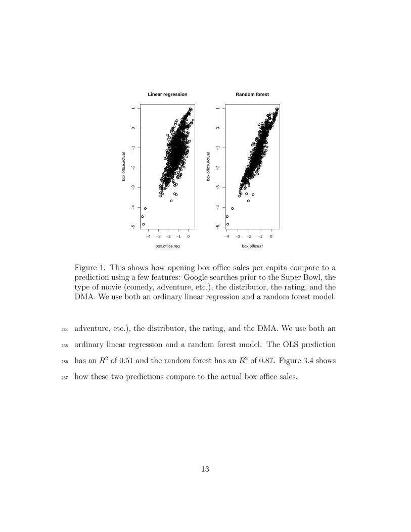
Figure 1: This shows how opening box office sales per capita compare to aprediction using a few features: Google searches prior to the Super Bowl, thetype of movie (comedy, adventure, etc.), the distributor, the rating, and theDMA. We use both an ordinary linear regression and a random forest model.
adventure, etc.), the distributor, the rating, and the DMA. We use both an234
ordinary linear regression and a random forest model. The OLS prediction235
has an R2 of 0.51 and the random forest has an R2 of 0.87. Figure 3.4 shows236
how these two predictions compare to the actual box office sales.237
13
4 Results for Google Searches238
4.1 First stage239
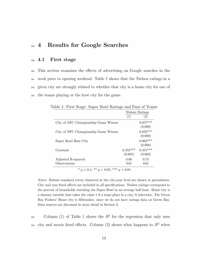
This section examines the effects of advertising on Google searches in the240
week prior to opening weekend. Table 1 shows that the Nielsen ratings in a241
given city are strongly related to whether that city is a home city for one of242
the teams playing or the host city for the game.243
Table 1: First Stage: Super Bowl Ratings and Fans of Teams
Nielsen Ratings(1) (2)
City of AFC Championship Game Winner 0.077***(0.009)
City of NFC Championship Game Winner 0.076***(0.008)
Super Bowl Host City 0.063***(0.008)
Constant 0.455*** 0.451***(0.004) (0.003)
Adjusted R-squared 0.66 0.75Observations 616 616
* p < 0.1; ** p < 0.05; *** p < 0.01
Notes: Robust standard errors clustered at the city-year level are shown in parentheses.
City and year fixed effects are included in all specifications. Nielsen ratings correspond to
the percent of households watching the Super Bowl in an average half hour. Home city is
a dummy variable that takes the value 1 if a team plays in a city; 0 otherwise. The Green
Bay Packers’ Home city is Milwaukee, since we do not have ratings data on Green Bay.
Data sources are discussed in more detail in Section 3.
Column (1) of Table 1 shows the R2 for the regression that only uses244
city and movie fixed effects. Column (2) shows what happens to R2 when245
14
Search index
Time
0 5 10 15 20 25 30
200
400
600
800
1000 Advertised
Not advertised
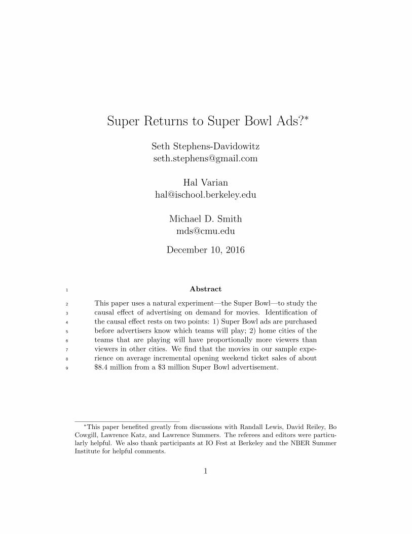
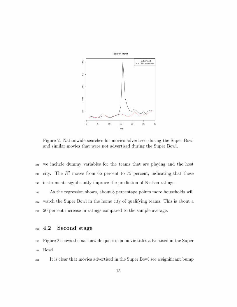
Figure 2: Nationwide searches for movies advertised during the Super Bowland similar movies that were not advertised during the Super Bowl.
we include dummy variables for the teams that are playing and the host246
city. The R2 moves from 66 percent to 75 percent, indicating that these247
instruments significantly improve the prediction of Nielsen ratings.248
As the regression shows, about 8 percentage points more households will249
watch the Super Bowl in the home city of qualifying teams. This is about a250
20 percent increase in ratings compared to the sample average.251
4.2 Second stage252
Figure 2 shows the nationwide queries on movie titles advertised in the Super253
Bowl.254
It is clear that movies advertised in the Super Bowl see a significant bump255
15
in searches. We also contrast these searches with national search volume for256
a set of placebo movies that had similar qualities to the advertising movies257
but did not advertise in the Super Bowl. We discuss how we select these258
movies in Section 6.3.259
While it is clear there is an increase in interest in advertising movies260
immediately after the ads are shown, it is not apparent how much of that261
initial interest translates into box office revenue. That question is what our262
model is designed to answer.263
The regression results in Table 2 use an ordinary least squares regression264
in Column (1) to show that, for movies that advertised in the Super Bowl,265
Google searches on release week are notably higher in cities with higher Super266
Bowl ratings than in other cities. Note that Google Trends numbers for the267
search volume in a particular geo are measured relative to the total number268
of searches in that geo. Hence the Trends numbers are already normalized269
for population size.270
Column (2) uses both home and host cities as instruments and finds about271
twice as large an effect as the OLS estimate. Our baseline model uses host272
cities as an instrument but Table 5 shows the estimated effect is similar if273
we use only home cities.274
16
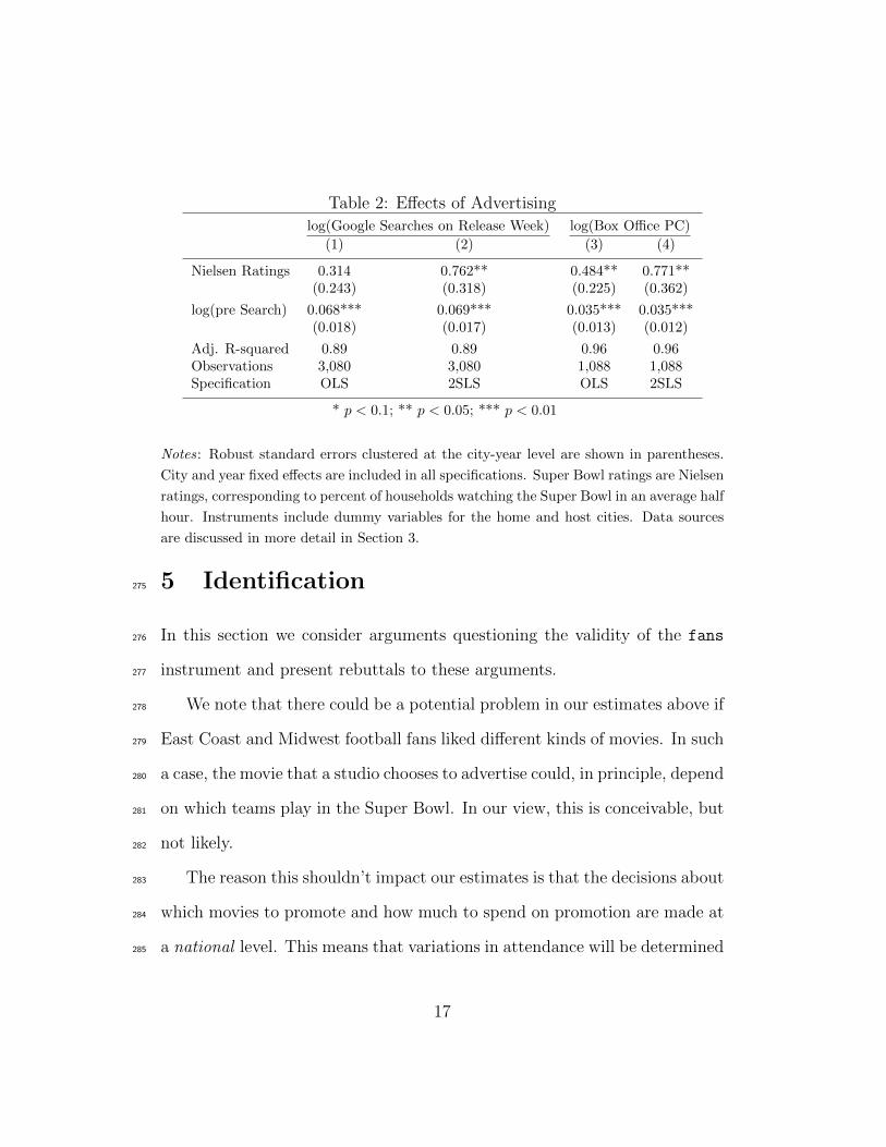
Table 2: Effects of Advertising
log(Google Searches on Release Week) log(Box Office PC)
(1) (2) (3) (4)
Nielsen Ratings 0.314 0.762** 0.484** 0.771**(0.243) (0.318) (0.225) (0.362)
log(pre Search) 0.068*** 0.069*** 0.035*** 0.035***(0.018) (0.017) (0.013) (0.012)
Adj. R-squared 0.89 0.89 0.96 0.96Observations 3,080 3,080 1,088 1,088Specification OLS 2SLS OLS 2SLS
* p < 0.1; ** p < 0.05; *** p < 0.01
Notes: Robust standard errors clustered at the city-year level are shown in parentheses.
City and year fixed effects are included in all specifications. Super Bowl ratings are Nielsen
ratings, corresponding to percent of households watching the Super Bowl in an average half
hour. Instruments include dummy variables for the home and host cities. Data sources
are discussed in more detail in Section 3.
5 Identification275
In this section we consider arguments questioning the validity of the fans276
instrument and present rebuttals to these arguments.277
We note that there could be a potential problem in our estimates above if278
East Coast and Midwest football fans liked different kinds of movies. In such279
a case, the movie that a studio chooses to advertise could, in principle, depend280
on which teams play in the Super Bowl. In our view, this is conceivable, but281
not likely.282
The reason this shouldn’t impact our estimates is that the decisions about283
which movies to promote and how much to spend on promotion are made at284
a national level. This means that variations in attendance will be determined285
17

primarily by local tastes. The only role that advertiser decisions might make286
is in determining which movies to advertise nationwide. This will typically287
not depend on which teams end up playing since the choice of which movies288
to advertise 1) is made well in advance and 2) has a tiny impact on the total289
size of the audience, as we establish below.290
5.1 Ad decisions are made in advance291
The decision to show an ad in the Super Bowl is typically made far in advance292
of the actual game, when advertisers would have little idea which teams would293
play. (They would know the host city, which we deal with shortly.) Table 3294
presents a list of press reports about the status of Super Bowl ad sales.295
(We report short URLs for reasons of space; complete URLs are provided296
in a spreadsheet in the Appendix.) Of course most advertisers do not wait297
until the last minute to purchase ads. According to our discussions with298
film industry executives, the decision about which movies to advertise in the299
Super Bowl are decided well in advance of the game. Generally studios only300
have a few choices of movies that will be released in an appropriate time301
frame, and a great deal of care goes into planning and executing marketing302
for the hoped-for blockbusters.303
18

Table 3: Ad sales for Super Bowl.
Year Snippet Date Source
2003 fewer than 10 spots available Jan 06 2003 superbowl.ads.com2004 –NA– –NA– –NA–2005 said Thursday all 59 slots had been sold Feb 02 2005 money.cnn.com2006 80% sold Dec 18 2005 www.mediapost.com2007 first half sold out Jan 03 2007 money.cnn.com2008 90% sold out by first week in Nov Nov 07 2007 money.cnn.com2009 much was sold out by September Jan 09 2008 money.cnn.com2010 had finished selling commercial time Feb 01 2010 articles.latimes.com2011 3 months before Oct 29 2010 adage.com2012 has sold out Jan 02 2012 www.bloomberg.com2013 advertisers need to announce 5 months out Sep 03 2013 www.usatoday.com
Notes: The columns show the Super Bowl year and extracts from news articles that
appeared on the indicated date from the indicated source. The full URL for these snippets
is available in the online Appendix.
5.2 Home-city and host-city effects are small304
It may well be that studios would advertise different movies in different ge-305
ographies if they were able to do so, but in this case there is a single nation-306
wide audience and advertisers must choose one movie for the entire audience.307
This restriction makes it implausible that the host cities and home cities of308
the teams playing in the Super Bowl would have any impact on advertising309
decisions since the aggregate audience for the ad is not very sensitive to which310
teams actually play and where they play.311
To see this, we constructed an estimate of what would have happened to312
viewership if the teams that lost the championship games instead won those313
games and competed in the Super Bowl.314
Consider for example, Pittsburgh’s 2005 loss. This meant that 161,000315
19
fewer households watched the ad in Pittsburgh than would have watched had316
Pittsburgh won. However, compared to the total viewership for the Super317
Bowl that year of 86 million this is only 0.2 percent, a tiny factor in an318
advertiser’s decision.319
The largest city in our sample is New York, but even in this case, the320
impact of the counterfactual is only 1.2 percent. Nationwide the average321
absolute difference in viewers across all DMAs and years was 0.4 percent of322
national viewership. Would the choice of ad to be shown in the Super Bowl323
depend on a 20 percent boost in viewership for 0.4 percent of the population?324
We believe that this effect is insignificant from an economic viewpoint and325
unlikely to affect studio decisions.326
A similar argument applies to the host cities which are known in advance.327
However, the population of the host cities comprise only 1.6 percent on av-328
erage of the DMAs in our sample. It seems implausible that choosing which329
movie ad to show nationwide in the Super Bowl would be influenced by a 0.2330
percent boost in viewership (1.6 percent of the population times a 15 percent331
boost).332
5.3 Expected fans333
Even though advertisers do not know with certainty who will play in the Su-334
per Bowl game, they can form judgments about who will play. Our contacts335
in the movie business tell us that decisions on which movies to advertise are336
made far in advance of the playoffs, and they would be highly unlikely to337
20
substitute at the last minute based on which teams were playing due to the338
major investments they have made in planning, publicity, and production of339
the movie ad. Furthermore, as we have seen, the effect on viewership of the340
movie ad is tiny.341
Nevertheless, let us take this critique seriously and see how plausible it is.342
Consider the Vegas odds for the AFC and NFC Championship games.3 We343
converted these odds to probabilities using the method described in Stern344
[1986] and calculated the expected fans for each city, where the expectation345
is made using the Vegas odds just prior to the championship game. We346
then used the expected fans as control variables in the regressions described347
earlier.348
We did not use the host city as an instrument since we thought that if349
advertisers were so sophisticated that they considered expected fans in their350
decisions, they would certainly take into account the host city in those deci-351
sions, which would make the host city an invalid instrument. The expected352
fans specification made no essential difference in the results.353
Let us summarize the argument. In our baseline specification, the instru-354
ment is whether a city’s team qualified for the Super Bowl. If advertisers355
were highly sophisticated and picked advertisements based on which teams356
were performing well up to the point they chose to advertise this could be357
a biased instrument. By controlling for the probability a team makes it to358
3These are available at http://www.vegasinsider.com/nfl/afc-championship/
history/.
21
the Super Bowl at the time of the Championship games, we ensure that our359
instrument is “as good as random.”360
5.4 Impact of outcome on subsequent ad spend361
If advertisers choose their subsequent ad spend on a movie based on the362
associated Super Bowl ratings, our instrument would not be valid. To check363
this possibility we ran a regression to see if local ad spend was associated364
with home and host cities. Our data on local ad spend is from Kantar Media,365
and these data were only available to us starting in 2009.366
The results of this regression are shown in Column 2 of Table 4. These367
estimates should be compared to those in Column 1 which is the first-stage368
regression from Table 1 but restricted to data from 2009 onward. Both de-369
pendent variables, the Nielsen ratings and ad spend per capita, are expressed370
in logs. Hence, the regression coefficients can be interpreted as percentage371
response. The impact of host and home cities on Nielsen ratings is large and372
statistically significant while the corresponding coefficients for local ad spend373
are small and statistically insignificant.374
6 Variations on the baseline model375
Here we consider a few variations on the baseline model.376
22
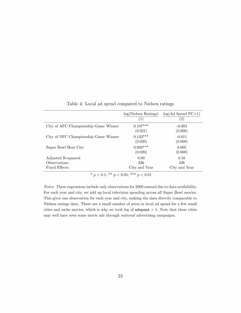
Table 4: Local ad spend compared to Nielsen ratings
log(Nielsen Ratings) log(Ad Spend PC+1)
(1) (2)
City of AFC Championship Game Winner 0.107*** -0.003(0.021) (0.008)
City of NFC Championship Game Winner 0.133*** -0.011(0.020) (0.008)
Super Bowl Host City 0.093*** 0.005(0.020) (0.008)
Adjusted R-squared 0.80 0.58Observations 336 336Fixed Effects City and Year City and Year
* p < 0.1; ** p < 0.05; *** p < 0.01
Notes: These regressions include only observations for 2009 onward due to data availability.
For each year and city, we add up local television spending across all Super Bowl movies.
This gives one observation for each year and city, making the data directly comparable to
Nielsen ratings data. There are a small number of zeros in local ad spend for a few small
cities and niche movies, which is why we took log of adspend + 1. Note that these cities
may well have seen some movie ads through national advertising campaigns.
23
4
8
12
16value
New.York.Giants
10
20
30value
San.Francisco.49ers
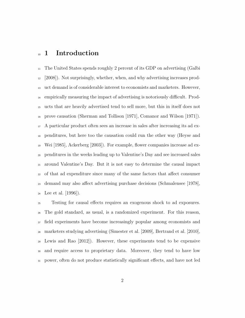
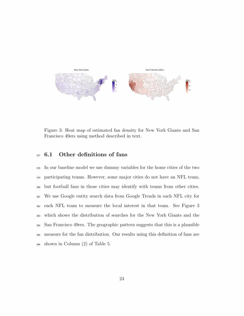
Figure 3: Heat map of estimated fan density for New York Giants and SanFrancisco 49ers using method described in text.
6.1 Other definitions of fans377
In our baseline model we use dummy variables for the home cities of the two378
participating teams. However, some major cities do not have an NFL team,379
but football fans in those cities may identify with teams from other cities.380
We use Google entity search data from Google Trends in each NFL city for381
each NFL team to measure the local interest in that team. See Figure 3382
which shows the distribution of searches for the New York Giants and the383
San Francisco 49ers. The geographic pattern suggests that this is a plausible384
measure for the fan distribution. Our results using this definition of fans are385
shown in Column (2) of Table 5.386
24
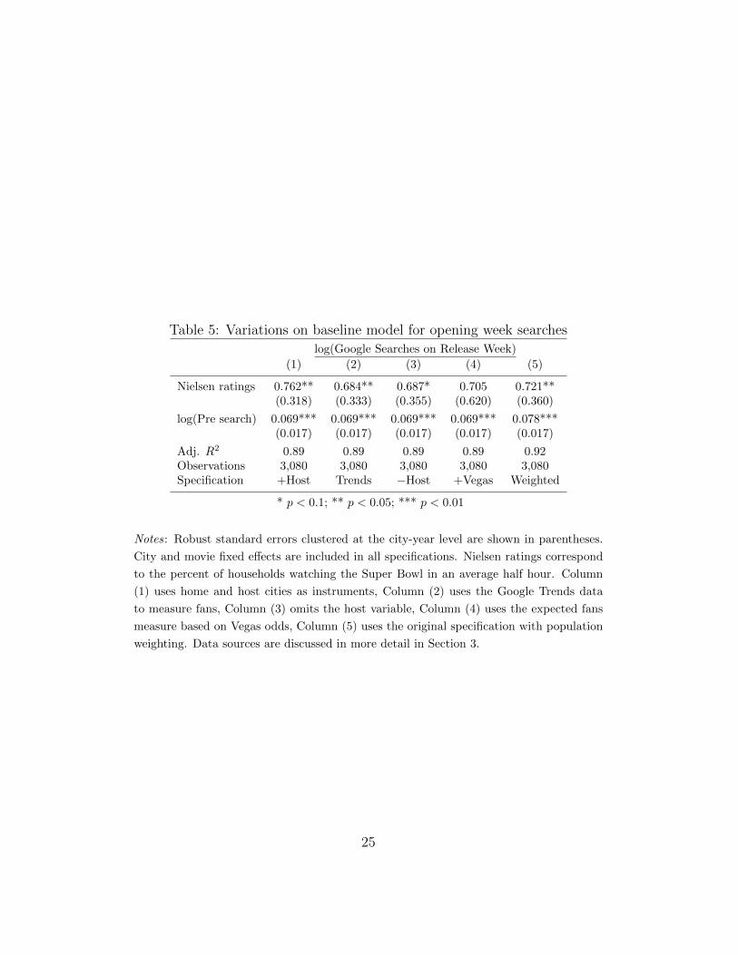
Table 5: Variations on baseline model for opening week searches
log(Google Searches on Release Week)
(1) (2) (3) (4) (5)
Nielsen ratings 0.762** 0.684** 0.687* 0.705 0.721**(0.318) (0.333) (0.355) (0.620) (0.360)
log(Pre search) 0.069*** 0.069*** 0.069*** 0.069*** 0.078***(0.017) (0.017) (0.017) (0.017) (0.017)
Adj. R2 0.89 0.89 0.89 0.89 0.92Observations 3,080 3,080 3,080 3,080 3,080Specification +Host Trends −Host +Vegas Weighted
* p < 0.1; ** p < 0.05; *** p < 0.01
Notes: Robust standard errors clustered at the city-year level are shown in parentheses.
City and movie fixed effects are included in all specifications. Nielsen ratings correspond
to the percent of households watching the Super Bowl in an average half hour. Column
(1) uses home and host cities as instruments, Column (2) uses the Google Trends data
to measure fans, Column (3) omits the host variable, Column (4) uses the expected fans
measure based on Vegas odds, Column (5) uses the original specification with population
weighting. Data sources are discussed in more detail in Section 3.
25
6.2 Opening weekend box office revenue387
As mentioned above, we have two measures of outcome: Google searches on388
the movie title and opening weekend revenue.389
The movie sales data we have is only available for a subset of cities. In390
particular, we only have data for movies that advertised in the Super Bowl391
and cities that were the home cities for teams that qualified for a Super Bowl392
or were the runners-up.393
Despite the smaller sample, there is evidence of a significant positive effect394
of Super Bowl ratings on movie sales as shown in Table 2, Columns (3) and395
(4). Note, though, that the effect on ticket sales is smaller than the effect on396
Google searches. This is true even if we use only the sub-sample of cities for397
which we have box office data. Table 6 reports regressions using the alternate398
definition of fans.399
6.3 Placebo analysis400
It is conceivable that Super Bowl ratings could influence subsequent movie401
attendance for all movies. We consider this possibility highly implausible,402
but decided to check it anyway.403
One could look at city-by-city movie attendance following the Super Bowl,404
but a better test is to look at movies that were similar to those advertised405
in the Super Bowl. Accordingly, we constructed a placebo set of movies. If406
watching the Super Bowl is correlated with subsequent overall movie atten-407
26
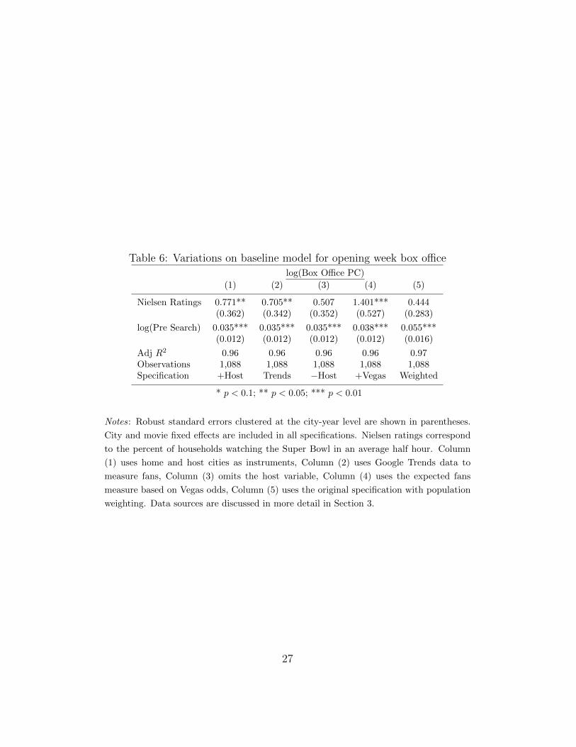
Table 6: Variations on baseline model for opening week box office
log(Box Office PC)
(1) (2) (3) (4) (5)
Nielsen Ratings 0.771** 0.705** 0.507 1.401*** 0.444(0.362) (0.342) (0.352) (0.527) (0.283)
log(Pre Search) 0.035*** 0.035*** 0.035*** 0.038*** 0.055***(0.012) (0.012) (0.012) (0.012) (0.016)
Adj R2 0.96 0.96 0.96 0.96 0.97Observations 1,088 1,088 1,088 1,088 1,088Specification +Host Trends −Host +Vegas Weighted
* p < 0.1; ** p < 0.05; *** p < 0.01
Notes: Robust standard errors clustered at the city-year level are shown in parentheses.
City and movie fixed effects are included in all specifications. Nielsen ratings correspond
to the percent of households watching the Super Bowl in an average half hour. Column
(1) uses home and host cities as instruments, Column (2) uses Google Trends data to
measure fans, Column (3) omits the host variable, Column (4) uses the expected fans
measure based on Vegas odds, Column (5) uses the original specification with population
weighting. Data sources are discussed in more detail in Section 3.
27

dance, we would expect to see it affect both those movies that were advertised408
and similar movies that weren’t advertised.409
Specifically, we used nearest-neighbor matching based on the movie bud-410
get, movie category (comedy, action, etc.), distributor, critic ratings, and411
year and month of release. We used the matchit R package which is specifi-412
cally designed for this purpose and described in detail in Ho et al. [2007a,b].413
We provide lists of the advertised and matched movies in the online appendix.414
In our view, these two lists appear to be similar.415
The results are shown in Table 7 for our baseline specification and a few of416
the variations considered above. What is noteworthy is that the coefficient417
on Nielsen ratings is insignificant for all specifications. Of course, the418
movies advertised in the Super Bowl were chosen for that distinction and our419
matching is far from perfect, so this analysis cannot be considered definitive420
evidence. Nevertheless, it is suggestive.421
We can test to see whether the estimated coefficient on ad views (Nielsen422
ratings) is different for the advertised and placebo movies. To do this we423
combine the two datasets and add an interaction term for Nielsen ratings424
and the advertised movies. This is denoted by Nielsen × Super Ad in425
Table 8. The interaction effect is significant at the 10 percent level in our426
baseline specification (Column 2) and at the 5 percent level when we use the427
Google Trends measure for fans (Column 3).4428
4Another question is whether placebo movies do worse than they would have if theSuper Bowl ads had not run. That is, does advertising for Super Bowl movies causesubstitution away from placebo movies? The relevant coefficient to test this is the firstone in Table 8, Nielsen Super Bowl Ratings. Unfortunately, we get different answers
28
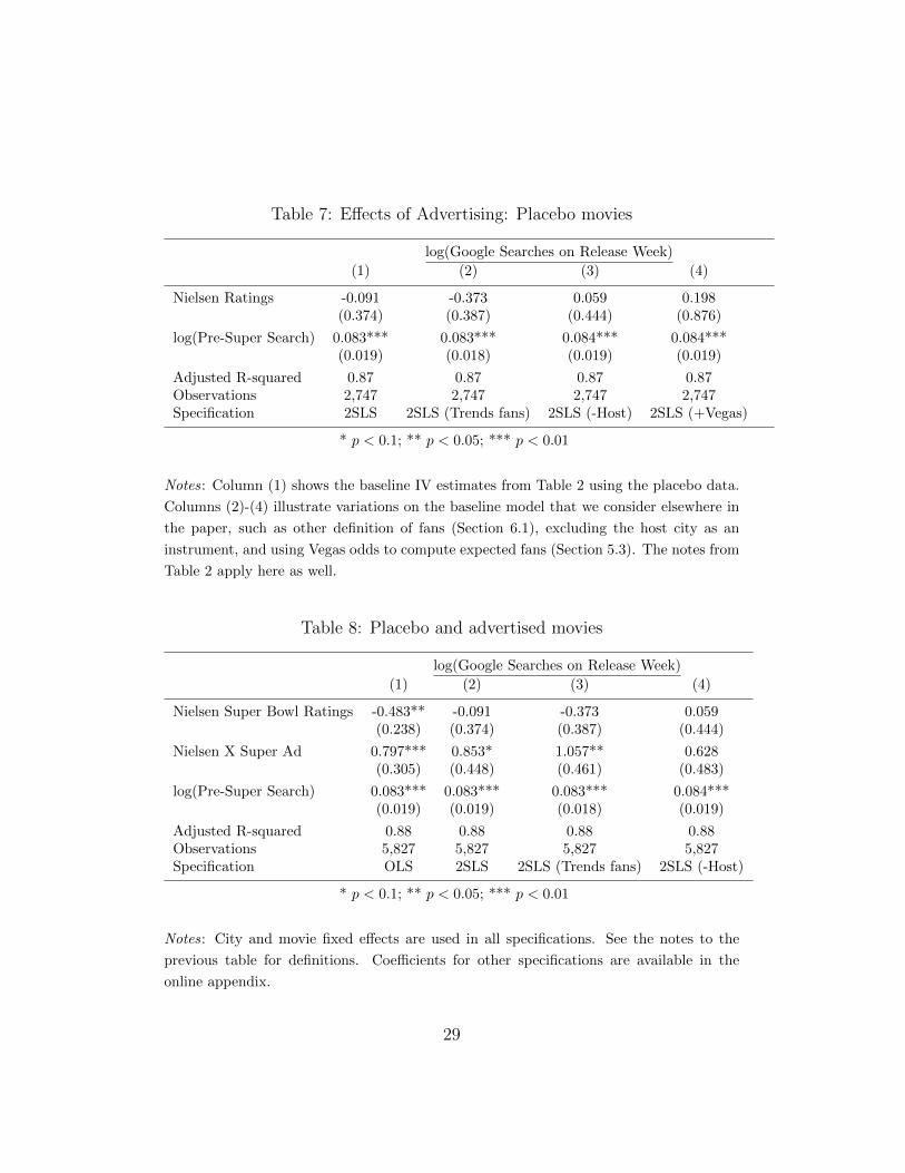
Table 7: Effects of Advertising: Placebo movies
log(Google Searches on Release Week)
(1) (2) (3) (4)
Nielsen Ratings -0.091 -0.373 0.059 0.198(0.374) (0.387) (0.444) (0.876)
log(Pre-Super Search) 0.083*** 0.083*** 0.084*** 0.084***(0.019) (0.018) (0.019) (0.019)
Adjusted R-squared 0.87 0.87 0.87 0.87Observations 2,747 2,747 2,747 2,747Specification 2SLS 2SLS (Trends fans) 2SLS (-Host) 2SLS (+Vegas)
* p < 0.1; ** p < 0.05; *** p < 0.01
Notes: Column (1) shows the baseline IV estimates from Table 2 using the placebo data.
Columns (2)-(4) illustrate variations on the baseline model that we consider elsewhere in
the paper, such as other definition of fans (Section 6.1), excluding the host city as an
instrument, and using Vegas odds to compute expected fans (Section 5.3). The notes from
Table 2 apply here as well.
Table 8: Placebo and advertised movies
log(Google Searches on Release Week)
(1) (2) (3) (4)
Nielsen Super Bowl Ratings -0.483** -0.091 -0.373 0.059(0.238) (0.374) (0.387) (0.444)
Nielsen X Super Ad 0.797*** 0.853* 1.057** 0.628(0.305) (0.448) (0.461) (0.483)
log(Pre-Super Search) 0.083*** 0.083*** 0.083*** 0.084***(0.019) (0.019) (0.018) (0.019)
Adjusted R-squared 0.88 0.88 0.88 0.88Observations 5,827 5,827 5,827 5,827Specification OLS 2SLS 2SLS (Trends fans) 2SLS (-Host)
* p < 0.1; ** p < 0.05; *** p < 0.01
Notes: City and movie fixed effects are used in all specifications. See the notes to the
previous table for definitions. Coefficients for other specifications are available in the
online appendix.
29
6.4 Interpretation429
The results suggest that an increase of 100 ratings points raises weekend430
ticket sales for a movie advertised on the Super Bowl by at least 50 per-431
cent. Note that 100 ratings points means a switch from 0 percent of people432
watching to 100 percent of people watching. In other words, it measures the433
difference from a hypothetical situation in which everybody watched the ad434
to a hypothetical situation in which nobody watched the ad.435
Since the Super Bowl averages about 42 ratings points overall, this implies436
that a Super Bowl ad increases release-week ticket sales by about 21 percent.437
In other words, the coefficient suggests there are 21 percent more ticket sales438
when 42 percent of the country watched the Super Bowl than there would439
have been if nobody watched the Super Bowl. The average movie in our440
sample took in $40 million on the opening weekend. Thus the incremental441
ticket revenue from the Super Bowl ad were roughly $8.4 million on average.442
Since a Super Bowl ad cost is about $3 million, this means an overall return443
of 2.8 to 1.444
According to industry practice, the studio typically pays for the entire445
marketing costs and receives 40-50 percent of the domestic box office revenue.446
(The exact numbers are closely guarded secrets, but see Danzig and Hughes447
[2014] for some estimates.) Hence the return to the studio from the Super448
Bowl ad is about 1.4 to 1, or a 40 percent ROI. 5449
depending on the specification. It is usually negative – suggesting there is substitution –but only statistically significant in one out of four main specifications.
5Hartmann and Klapper [2015] estimate a 153 percent ROI for Super Bowl beer ads,
30
We want to emphasize four caveats in interpreting these results.450
First, this back of the envelope calculation ignores future revenue streams451
such as ticket sales after the opening weekend and other revenue through452
home movie purchases, TV licensing, and so on. Some of this additional453
revenue may be attributable to the Super Bowl ad impressions, though we454
have no easy way to measure this.455
However, a causal relationship between increased movie attendance and456
increased home entertainment sales is consistent with Choi et al. [2015] who457
use opening-weekend snowstorms as an instrument and find that a 10 percent458
rise in theatrical attendance causes an 8 percent increase in DVDs/Blu-ray459
sales when they are released. Cable licensing deals are also directly tied to460
box office success so that any increase in box office revenue will positively461
impact revenue from this channel.462
We also do not know how the incremental revenue is divided among the463
various parties—how much goes to the studios, producers, writers, stars,464
and so on. Similarly, we don’t know exactly how the costs of the Super Bowl465
ad are divided among the various parties. However, as indicated above, it466
appears that studios are the primary decision makers with respect to Super467
Bowl ads and bear most of the marketing costs.468
Second, in calculating the return to advertising, we are assuming that the469
incremental viewers of the Super Bowl have the same response to ads as those470
who would watch the Super Bowl anyway. It is possible that the committed471
but caution that this is a likely an overestimate.
31

fans pay more attention to the game and less to ads. Or perhaps they are472
much more engaged with the entire experience and so pay more attention473
to ads than the incremental viewers. It is also possible that the incremental474
fans have substantially different tastes in movies than the fans you would get475
simply by purchasing more ad slots. We provide some evidence on this in476
Section 7.477
Third, we don’t know how these results extend to other settings, as the478
Super Bowl has unique qualities. There are other similar events such as the479
World Series, basketball playoffs, the Summer and Winter Olympics, and so480
on. These natural experiments are not quite as clean-cut as the Super Bowl,481
but are certainly worthy of future study.482
Fourth, one might ask why the estimated return is so high. First, it483
is important to understand that our results pertain to returns on movies484
that the studio has chosen to advertise on the Super Bowl. The return on485
advertising movies with mediocre prospects could be much lower. Second,486
once the network has set a market-clearing price, we would expect that the487
marginal ad would earn a normal, risk-adjusted rate of return. However,488
the average ad would typically earn a return higher than the marginal ad.489
One might then ask “if the return to the movie ad is so high, why don’t the490
studios advertise more movies?” The answer to this question may be that491
they only have a few movies for which a Super Bowl ad makes economic492
sense. Movie theaters can only show a limited number of movies at any one493
time, and the conventional wisdom in the industry is that if two blockbusters494
32
are released on the same weekend, the revenues of both movies will suffer.495
As a result, studios typically try to stagger the release of blockbusters, so at496
any one time there are only a few movies that would warrant Super Bowl497
treatment. Whatever the explanation, we typically see only 6-8 movie ads498
per Super Bowl and this number does not vary much from year to year.499
Finally, we want to clarify how these results fit with the Super Bowl500
Impossibility Theorem (Lewis and Rao [2012]). They argue that it is nearly501
impossible for a firm to test the effects of an individual ad campaign, even if it502
randomly assigned DMAs during a Super Bowl. How, then, can we find such503
highly statistically significant results? The answer is that the Super Bowl504
Impossibility Theorem refers to the question of measuring the effectiveness505
of a single campaign. But here, we study the average effect of 70 campaigns.506
The noise level is too high to say anything about the effects of a particular507
advertisement, but the average performance of all movies in our sample can508
be estimated reasonably precisely.509
7 Heterogeneous treatment effects510
We have shown that the incremental ad exposures due to the home-team511
effect have a causal impact on both Google queries and opening weekend512
revenue. This suggest that increased ad expenditure would also have an513
incremental impact on these outcomes. However, the incremental ad views514
from the home-team effect may well be different than the incremental ad515
33

views from simply spending more money on advertising.516
We can offer some suggestive evidence on this point. We ran a Google517
Consumer Survey and asked the 2,568 respondents whether they watched518
the Super Bowl on TV in 2013, 2014 or both years. The question of interest519
was whether those who watched both years were different than those who520
watched only one year. The dimensions on which the respondents could differ521
were inferred age, gender, and income.6522
We found that those who watched the Super Bowl in both years, rather523
than a single year, tended to be older, more male, and live in wealthier areas.524
However, most of these effects tended to be statistically insignificant, with525
the exception of gender. We suspect that there is some difference between the526
incremental viewers from the home-city effect and the incremental viewers527
that would be reached by increased ad spend.528
Nevertheless, we believe that our estimates can be useful in estimating529
the response to ad spend. Suppose that a movie advertiser targeted its ads to530
reflect the audience composition of the incremental Super Bowl viewers. This531
targeting could be informed by a more sophisticated version of our survey.532
That advertiser might well expect a response to its ad spend along the lines533
of that described in Section 6.2. So those estimates of the impact of spend534
on box office should be a lower bound on what ad effectiveness would be if535
ad targeting could be fully optimized.536
6Inferred age and gender are based on web site visits and inferred income is based onthe IP address of the respondent and Census data.
34

We also can test whether there are differential effects based on when a537
movie is released. Are ads less effective for movies released well after the538
Super Bowl? We divided our sample into movies with release dates more539
than 70 days out and those with release dates less than 70 days out. We540
recreated the regressions in Table 2. Somewhat surprisingly, we did not see541
a difference in the effects of ads on box office sales in these two groups.7542
8 Discussion543
We use a natural experiment—the Super Bowl—to study the causal effect544
of advertising on movie demand. Our identification strategy relies on the545
fact that Super Bowl ads are purchased before advertisers know which teams546
will play in the Super Bowl and that cities where there are many fans of the547
qualifying teams have substantially larger viewership than other cities do.548
Within this setting we study 70 movies that were advertised during the549
2004-2014 Super Bowls. We compare product purchase patterns for adver-550
tised movies in cities with fans from the qualifying teams to cities with fans551
of near-qualifying teams. We find a substantial increase in opening weekend552
revenue due to Super Bowl advertisements. On average, the movies in our553
sample experience an incremental increase of $8.4 million in opening weekend554
7In general, we don’t have sufficient power to break down the treatment effects. Thereare several other interesting questions, such as whether there are differential effects formovies with more competition, but we have to leave these questions for further research.It may be possible to investigate such issues after we accumulate a few more years of SuperBowl data.
35
box office revenue from a $3 million Super Bowl advertisement.555
We suggest that our methodology can be generalized to a variety of sports556
settings where the nature of qualifying creates a large random shock to ad557
viewership in a particular area, and that this methodology has notable ad-558
vantages compared to the more common approach of using field experiments559
to determine the causal impact of advertising. The best identification comes560
from sporting events such as the Super Bowl in which the teams that will play561
are unknown at the time companies purchase advertising spot. However, even562
if the home cities are known it seems to us unlikely that advertisers would563
take this information into account when choosing its ad expenditure. So the564
methodology could well be applicable for a broader set of media broadcasts565
with differential appeal across geographies.566
36
References567
Daniel A. Ackerberg. Advertising, Learning, and Consumer Choice in Ex-568
perience Good Markets: an Empirical Examination. International Eco-569
nomic Review, 44(3):1007–1040, August 2003. ISSN 0020-6598. doi:570
10.1111/1468-2354.t01-2-00098. URL http://doi.wiley.com/10.1111/571
1468-2354.t01-2-00098.572
Marianne Bertrand, Dean Karlan, Sendhil Mullainathan, Eldar Shafir,573
and Jonathan Zinman. What’s Advertising Content Worth? Ev-574
idence from a Consumer Credit Marketing Field Experiment.575
The Quarterly Journal of Economics, 125(1):44, 2010. URL576
http://www.ingentaconnect.com.ezp-prod1.hul.harvard.edu/577
content/oup/qje/2010/00000125/00000001/art00007.578
Patrick Choi, Peter Boatwright, and Michael D. Smith. The perfect storm:579
Using snowstorms to analyze the effect of theatrical attendance on de-580
mand for subsequently released DVDs. Technical report, Carnegie Mellon581
University, 2015. URL http://ssrn.com/abstract=2639303.582
William S Comanor and Thomas A Wilson. On Advertising and583
Profitability. The Review of Economics and Statistics, 53(4):408–10,584
1971. URL http://econpapers.repec.org/RePEc:tpr:restat:v:53:585
y:1971:i:4:p:408-10.586
Scott Danzig and Mark Hughes. Breakdown of587
movie costs, 2014. URL http://www.quora.com/588
What-is-the-breakdown-of-costs-associated-with-making-a-high-budget-Hollywood-film.589
Douglas Galbi. U.S. Annual Advertising Spending Since 1919, 2008. URL590
http://www.galbithink.org/ad-spending.htm.591
Wesley R. Hartmann and Daniel Klapper. Super Bowl ads. Technical report,592
Stanford Graduate School of Business, 2015. URL http://faculty-gsb.593
stanford.edu/hartmann/SuperBowl.pdf. First version presented at IN-594
FORMS Marketing Science, June 7-9, 2012.595
Joseph F. Heyse and William W. S. Wei. Modelling the Advertising-Sales596
Relationship through Use of Multiple Time Series Techniques. Journal597
of Forecasting, 4(2):165–181, 1985. ISSN 02776693. doi: 10.1002/for.598
3980040206. URL http://doi.wiley.com/10.1002/for.3980040206.599
37
Daniel Ho, Kosuke Imai, Gary King, and Elizabeth Stuart. Matching as600
nonparametric preprocessing for reducing model dependence in parametric601
causal inference. Political Analysis, 2007a. URL http://gking.harvard.602
edu/files/abs/matchp-abs.shtml.603
Daniel Ho, Kosuke Imai, Gary King, and Elizabeth Stuart. Matchit: Non-604
parametric preprocessing for parametric causal inference. Journal of Statis-605
tical Software, 15(3):199–236, 2007b. URL http://gking.harvard.edu/606
matchit/.607
Jason Ho, Tirtha Dhar, and Charles Weinberg. Playoff payoff: Super Bowl608
advertising for movies. International Journal of Research in Marketing,609
26:168–179, 2009. URL www.elsevier.com/locate/ijresmar.610
Ye Hu, Leonard M. Lodish, and Abba A. Krieger. An Analysis of Real World611
TV Advertising Tests: a 15-Year Update. Journal of Advertising Research,612
47(3):341–353, 2007.613
Junsoo Lee, B. S. Shin, and In Chung. Causality Between Advertising and614
Sales: New Evidence from Cointegration. Applied Economics Letters, 3(5):615
299–301, 1996. ISSN 1350-4851. URL http://econpapers.repec.org/616
RePEc:taf:apeclt:v:3:y:1996:i:5:p:299-301.617
Randall A. Lewis and Justin M. Rao. On the Near Impossibility of Measuring618
Advertising Effectiveness. Working Paper, 2012.619
Randall Aaron Lewis and David H. Reiley. Does Retail Advertising Work?620
Measuring the Effects of Advertising on Sales Via a Controlled Experiment621
on Yahoo! SSRN Electronic Journal, June 2008. ISSN 1556-5068. doi:622
10.2139/ssrn.1865943. URL http://papers.ssrn.com.ezp-prod1.hul.623
harvard.edu/abstract=1865943.624
Rui Miao and Yueyue Ma. The dynamic impact of websearch volume on625
product — an empirical study based on box office revenues. WHICEB 2015626
Proceedings, 2015. URL http://aisel.aisnet.org/whiceb2015/14.627
Reggie Panaligan and Andrea Chen. Quantifying movie magic with google628
search. Google Think Insights, 2013. URL http://ssl.gstatic.com/629
think/docs/quantifying-movie-magic_research-studies.pdf.630
38
Richard Schmalensee. A Model of Advertising and Product Quality. Journal631
of Political Economy, 86(3):485–503, 1978. URL http://ideas.repec.632
org/a/ucp/jpolec/v86y1978i3p485-503.html.633
Roger Sherman and Robert D. Tollison. Advertising and Prof-634
itability. The Review of Economics and Statistics, 53(4):397–407,635
1971. URL http://econpapers.repec.org/RePEc:tpr:restat:v:53:636
y:1971:i:4:p:397-407.637
Duncan Simester, Yu Hu, Erik Brynjolfsson, and Eric T. Anderson. Dynam-638
ics of Retail Advertising: Evidence from a Field Experiment. Economic639
Inquiry, 47(3):482–499, 2009. ISSN 0095-2583. URL http://econpapers.640
repec.org/RePEc:bla:ecinqu:v:47:y:2009:i:3:p:482-499.641
Hal Stern. The probability of winning a football game as a function of the642
pointspread. Technical report, Department of Statistics, Stanford Univer-643
sity, 1986.644
Rama Yelkur, CHuck Tomkovick, and Patty Traczyk. Super Bowl advertising645
effectiveness: Hollywood finds the games golden. Journal of Advertising646
Research, 44(1):143–159, 2004. URL http://journals.cambridge.org/647
abstract_S0021849904040085.648
39
Recommended