Quarterly Reviews of Biophysics , (), pp. – Printed in the United Kingdom
# Cambridge University Press
Structure calculation of biological
macromolecules from NMR data
PETER GU> NTERT
Institut fuX r Molekularbiologie und Biophysik, EidgenoX ssische Technische Hochschule, CH-���� ZuX rich,
Switzerland
.
.
.
.
. Nuclear Overhauser effects
. Scalar coupling constants
. Hydrogen bonds
. Chemical shifts
. Residual dipolar couplings
. Other sources of conformational restraints
.
. Systematic analysis of local conformation
. Stereospecific assignments
. Treatment of distance restraints to diastereotopic protons
. Removal of irrelevant restraints
.
. Metric matrix distance geometry
. Variable target function method
. Molecular dynamics in Cartesian space
. Torsion angle dynamics
.. Tree structure of the molecule
.. Potential energy
.. Kinetic energy
.. Torsional accelerations
.. Integration of the equations of motion
.. Energy conservation and time step length
.. Simulated annealing schedule
.. Computation times
.. Application to biological macromolecules
. Other algorithms

Peter GuX ntert
.
. Restraint violations
. Atomic root-mean-square deviations
. Torsion angle distributions
. Hydrogen bonds
. Molecular graphics
. Check programs
. A single, representative conformer
.
. Ensemble size
. Different NOE calibrations
. Completeness of the data set
. Wrong restraints and their elimination
.
. Chemical shift tolerance range
. Semiautomatic methods
. Ambiguous distance restraints
. Iterative combination of NOE assignment and structure calculation
.
. Restrained energy minimization
. Molecular dynamics simulation
. Time- or ensemble averaged restraints
. Relaxation matrix refinement
.
.
.
The relationship between amino acid sequence, three-dimensional structure and
biological function of proteins is one of the most intensely pursued areas of
molecular biology and biochemistry. In this context, the three-dimensional
structure has a pivotal role, its knowledge being essential to understand the
physical, chemical and biological properties of a protein (Branden & Tooze, ;
Creighton, ). Until structural information at atomic resolution could
only be determined by X-ray diffraction techniques with protein single crystals
(Drenth, ). The introduction of nuclear magnetic resonance (NMR)
spectroscopy (Abragam, ) as a technique for protein structure determination
(Wu$ thrich, ) has made it possible to obtain structures with comparable
accuracy also in a solution environment that is much closer to the natural situation
in a living being than the single crystals required for protein crystallography.
The NMR method for the study of molecular structures depends on the
sensitive variation of the resonance frequency of a nuclear spin in an external
magnetic field with the chemical structure, the conformation of the molecule, and
the solvent environment (Ernst et al. ). The dispersion of these chemical
Structure calculation of biological macromolecules
shifts ensures the necessary spectral resolution, although it usually does not
provide direct structural information. Different chemical shifts arise because
nuclei are shielded from the externally applied magnetic field to differing extent
depending on their local environment. Three of the four most abundant elements
in biological materials, hydrogen, carbon and nitrogen, have naturally occurring
isotopes with nuclear spin "
#, and are therefore suitable for high-resolution NMR
experiments in solution. The proton ("H) has the highest natural abundance
(±%) and the highest sensitivity (due to its large gyromagnetic ratio) among
these isotopes, and hence plays a central role in NMR experiments with
biopolymers. Because of the low natural abundance and low relative sensitivity of
"$C and "&N (±% and ±%, respectively) NMR spectroscopy with these
nuclei normally requires isotope enrichment. This is routinely achieved by
overexpression of proteins in isotope-labelled media. Structures of small proteins
with molecular weight up to kDa can be determined by homonuclear "H NMR.
Heteronuclear NMR experiments with "H, "$C and "&N (Cavanagh et al. ) are
indispensable for the structure determination of larger systems (e.g. Clore &
Gronenborn, ; Edison et al. ).
Today many, if not most, NMR measurements with proteins are performed
with the ultimate aim of determining their three-dimensional structure. However,
NMR is not a ‘microscope with atomic resolution’ that would directly produce an
image of a protein. Rather, it is able to yield a wealth of indirect structural
information from which the three-dimensional structure can only be uncovered by
extensive calculations. The pioneering first structure determinations of peptides
and proteins in solution (e.g. Arseniev et al. ; Braun et al. ; Clore et al.
b ; Williamson et al. ; Zuiderweg et al. ) were year-long struggles,
both fascinating and tedious because of the lack of established NMR techniques
and numerical methods for structure calculation, and hampered by limitations of
the spectrometers and computers of the time. Recent experimental, theoretical
and technological advances – and the dissemination of the methodological
knowledge – have changed this situation decisively: Given a sufficient amount of
a purified, water-soluble, monomeric protein with less than about amino acid
residues, its three-dimensional structure in solution can be determined routinely
by the NMR method, following the procedure described in the classical textbook
of Wu$ thrich () and outlined in Fig. .
There is a close mutual interdependence, indicated by circular arrows in Fig. ,
between the collection of conformational restraints and the structure calculation,
which forms the subject of this work. In its framework, structure calculation is the
de novo computation of three-dimensional molecular structures on the basis of
conformational restraints derived from NMR. Structure calculation is
distinguished from structure refinement by the fact that no well-defined start
conformation is used, whereas structure refinement aims at improving a given,
well-defined structure with respect to certain features, for example its
conformational energy.
After a historical outline of the development of NMR structure calculation
methods in Section , and an overview of NMR structures deposited in the Protein

Peter GuX ntert
Protein sample
NMR spectroscopy
Processing of NMR data
Sequential resonance assignment
Collection of conformational restraints
Structure calculation
Structure refinement
Structure analysis
Fig. . Outline of the procedure for protein structure determination by NMR.
Data Bank in Section , the core part of the presentation starts in Section with
a discussion of various types of structurally relevant NMR data and their
conversion into conformational restraints. Section explains preliminary steps
that precede a structure calculation. The central Section is devoted to algorithms
used for structure calculation. Special emphasis is given to molecular dynamics in
torsion angle space, the currently most efficient method for biomolecular structure
calculation. Measures to analyse the outcome of a structure calculation are
introduced in Section . The relation between the conformational restraints in the
input of a structure calculation and the quality of the resulting structure is
discussed in Section . The combination of NOE assignment and structure
calculation in automated procedures is introduced in Section . The text concludes
with a glance at various structure refinement methods in Section .
.
The aim of this section is to give a brief overview of the history of NMR structure
calculation in the period from its beginning in the early s until now. No
attempt is made to cover the history of NMR spectroscopy in general, or of other
aspects of the NMR method for biomolecular structure determination besides
structure calculation, since a lavish account of this exciting story has been
published recently in the opening volume of the Encyclopedia of NMR (Grant &
Harris, ), together with an entertaining collection of personal reminiscences
from the pioneers in the field. The new method was confronted initially with much
scepticism and also utter disbelief, partly because the early solution structure
determinations were done for systems for which the three-dimensional structure
had already been known, or could be inferred from that of a homologous protein.
Structure calculation of biological macromolecules
Suspicions could be allayed only when simultaneous but completely independent
determinations of the three-dimensional structure of the protein tendamistat, for
which no structural information was available before the project was started, by
X-ray crystallography (Pflugrath et al. ) and by NMR (Kline et al. ,
) yielded virtually identical results (Billeter et al. ).
In the early development of the NMR method for protein structure
determination it became clear that computer algorithms for structure calculation
would be an indispensable prerequisite for solving the three-dimensional
structures of objects as complex as a protein. It emerged that the key data
measured by NMR would consist of a network of distance restraints between
spatially proximate hydrogen atoms (Dubs et al. ; Kumar et al. ), for
which existing techniques for structure determination from X-ray diffraction data
would be inappropriate. Manual model building or interactive computer graphics
could not provide solutions either because the intricacies of the distance restraint
network precluded a manual analysis at atomic level, virtually restricting manual
approaches to strongly simplified, cartoon-like representations of a protein
(Zuiderweg et al. ). Hence new ways had to be developed.
The mathematical theory of distance geometry (Blumenthal, ) was the first
method to be used for protein structure calculation. (Since distance geometry was
first, NMR structure calculations were and are often termed ‘distance geometry
calculations’, regardless of the principles underlying the algorithm used. Here,
this practice is not followed, and the term is used only for algorithms based on
distance space and the metric matrix.) The basic idea of distance geometry is to
formulate the problem not in the Cartesian space of the atom positions but in the
much higher dimensional space of all interatomic distances where it is
straightforward to find configurations that satisfy a network of distance
measurements. The crucial step is then the embedding of a solution found in
distance space into Cartesian space. Algorithms for this purpose had been devised
(Crippen, ; Crippen & Havel, ; Havel et al. ; Kuntz et al. )
already before their use in NMR protein structure determination could be
envisioned, but the advent of NMR as a – however imprecise – microscopic ruler
with which a large number of interatomic distances could be measured in a
biological macromolecule spurred vigorous research in the field of distance
geometry. For the first time a computer program was used to calculate the solution
structure of a biological macromolecule on the basis of NOE measurements
(Braun et al. ). The program, based on metric matrix distance geometry, was
applied to a nonapeptide of atoms. distance restraints had been determined
by NMR. Later, the same program was used for the first calculation of the NMR
solution structure of a globular protein, a scorpion insectotoxin of amino acid
residues comprising both α-helical and β-sheet secondary structure (Arseniev et
al. ). Presumably because of memory limitations, not all atoms of the protein
could be treated explicitly. Instead, a simplified representation with two
pseudoatoms per residue was used. Havel, Kuntz & Crippen () provided an
improved version of the original embedding algorithm, which was implemented
in (Havel & Wu$ thrich, ), the first complete program package for NMR

Peter GuX ntert
protein structure calculation. Calculations with simulated NMR data sets (Havel
& Wu$ thrich, ), and a structure calculation of a protein on the basis of
experimental NMR data (Williamson et al. ), both performed with ,
made it clear that even very imprecise measurements of distances that are short
compared with the size of a protein were sufficient to define the three-dimensional
structure of a protein, provided that a sufficient number of such distance restraints
was available. At the time this finding convincingly refuted a widespread
argument against NMR protein structure determination, namely that short
distance restraints could never consistently determine the relative orientation of
parts of a molecule that are much further apart than the longest upper distance
bound.
For a molecular system with N atoms, metric matrix distance geometry calls for
storage of a matrix with N# elements, and the computation time is proportional to
N$. Both requirements posed formidable challenges to the computer hardware in
these early years of protein structure calculation. Even for a small protein like the
basic pancreatic trypsin inhibitor (BPTI), with amino acid residues and about
atoms, special devices had to be introduced to cut down the number of atoms
in the embedding step such as performing the embedding on only a substructure.
Nevertheless, the computation time for a single BPTI conformer was of the order
of hours on a DEC , then a state-of-the-art computer (Havel & Wu$ thrich,
). The program was in use for several years, and it could have been
expected that such practical problems would be alleviated by the steady
advancement of computer technology. However, other, more fundamental
problems were looming.
In the meantime algorithms based on very different ideas came into being. The
problem of finding molecular conformations that are in agreement with certain
geometrical restraints can always be formulated as one of minimization of a
suitable objective or target function. The global minimum of the target function,
or a close enough approximation of it, is sought, whereas local minima are to be
avoided. The target function can be defined on different spaces. Metric matrix
distance geometry took refuge from the local minimum problem in a very high-
dimensional space, from which it could be difficult at times to come back to our
three-dimensional world, not least because the notions of chirality or mirror
images are unknown in distance space. Another approach went the opposite way
by reducing the dimensionality of conformation space as far as possible.
Recognizing that fluctuations of the covalent bond lengths and bond angles
around their equilibrium values are small and fast, and cannot be measured by
NMR, Braun & Go () retained only the essential degrees of freedom of a
macromolecule, namely the torsion angles. In this way, the number of degrees of
freedom was reduced by about an order of magnitude compared with Cartesian
coordinate space. Their variable target function method in torsion angle space
(Braun & Go, ) used the method of conjugate gradients (Powell, ), a
standard algorithm for the minimization of a multidimensional function. In the
times of severely limited computer memories this algorithm had the advantage
that no large matrices had to be stored. However, two problems had to be

Structure calculation of biological macromolecules
overcome to enable its use in protein structure calculation. For efficient
minimization it is essential to know not only the value of the target function but
also its gradient, that is the partial derivatives with respect to the coordinates, the
torsion angles in this case. At first the calculation of the gradient appeared to be
very computation intensive. However, Abe et al. () had removed this obstacle
with their discovery of a fast recursive method to accomplish this task. The other,
more daunting difficulty was the local minimum problem. Being a minimizer that
takes exclusively downhill steps, the conjugate gradient algorithm is effective in
locating a local minimum in the vicinity of the current conformation, but not as
a method to search conformation space for the global minimum of the target
function. Therefore, straightforward conjugate gradient minimization of a target
function representing the complete network of NMR-derived restraints and the
steric repulsion among all pairs of atoms in a protein was found to get stuck
virtually always in local minima very far from the correct solution. The variable
target function method, devised by Braun & Go (), and implemented in their
program , offered a partial answer to this question by going through a
series of minimizations of different target functions that gradually included
restraints between atoms further and further separated along the polypeptide
chain, thereby increasing step-by-step the complexity of the target function. This
was a natural idea for helical proteins, where first, under the influence of short-
and medium-range distance restraints, the helical segments are formed and
subsequently, when the long-range restraints gradually come into play, positioned
relative to each other. Not surprisingly, the variable target function method
performed well for helical peptides but much less so for β-sheet proteins like
tendamistat, where the fraction of acceptable conformers dropped to % (Kline
et al. ) ; a situation that was calling for enhancements of the original variable
target function idea. Reassuring, on the other hand, was the result obtained in the
course of the solution structure determination of BPTI, where both algorithms,
and , yielded essentially equivalent structure bundles, both in close
agreement with the X-ray structures (Wagner et al. ).
In parallel with these developments, another powerful computing technique
was recruited for protein structure calculation: molecular dynamics simulation.
The method is based on classical mechanics and proceeds by numerically solving
Newton’s equation of motion in order to obtain a trajectory for the molecular
system. The Cartesian coordinates of the atoms are the degrees of freedom. In the
context of protein structure calculation the basic advantage of molecular dynamics
simulation over minimization techniques is the presence of kinetic energy. It
allows the system to escape from local minima that would be traps for minimizers
bound to take exclusively downhill steps. By , molecular dynamics simulation
had existed already for more than two decades. Initially it had been used to
simulate simple gases (Alder & Wainwright, ; Rahman, ; Verlet, ),
but calculations with proteins had become feasible as well, starting with the first
simulation of BPTI by McCammon et al. (). The first calculation of protein
tertiary structure on the basis of NMR distance measurements by molecular
dynamics simulation was performed by Kaptein et al. () for the lac repressor

Peter GuX ntert
headpiece, using the program that was to become (van Gunsteren &
Berendsen, ). This was, however, not really a de novo structure calculation by
molecular dynamics simulation because first ‘a molecular model was built using
the three helices as building blocks […] which, after measurement of the atomic
co-ordinates, was subjected to refinement’ (Kaptein et al. ). Clore et al.
() used the molecular dynamics program (Brooks et al. ) to
compute the solution structure of a single helix of amino acid residues, starting
from three different initial conformations, an α-helix, a β-strand, and a "!
-helix.
The viability of restrained molecular dynamics simulation as a method for de novo
structure calculation of complete globular proteins was demonstrated by Bru$ nger
et al. (), using simulated data for crambin, a small protein of amino acid
residues. Shortly thereafter, a method that has been in use for NMR structure
calculation ever since was introduced and employed to calculate the globular
structure of a protein with amino acids (Clore et al. b) : the combination
of metric matrix distance geometry to obtain a rough but correctly folded
structure followed by restrained energy minimization and molecular dynamics
refinement.
So far, these molecular dynamics approaches had relied on a full empirical force
field (Brooks et al. ) to ensure proper stereochemistry, and were generally
run at a constant temperature, close to room temperature. Substantial amounts of
computation time were required because the empirical energy function included
long-range pair interactions that were time-consuming to evaluate, and because
conformation space was explored slowly at room temperature. Both features had
been inherited from molecular dynamics programs created with the aim of
simulating the time evolution of a molecular system as realistically as possible in
order to extract from the complete trajectories molecular quantities of interest.
When these algorithms are used for structure calculations, however, the objective
is quite different. Here, they simply provide a means to efficiently optimize a
target function that takes the role of the potential energy. The course of the
trajectory is unimportant, as long as its end point comes close to the global
minimum of the target function. Therefore, the efficiency of a structure calculation
by molecular dynamics can be enhanced by modifications of the force field or the
algorithm that do not significantly alter the location of the global minimum (the
correctly folded structure) but shorten (in terms of the number of integration steps
needed) the trajectory by which it can be reached from the start conformation.
Based on this observation new ingredients to the method made the folding process
much more efficient (Nilges et al. a, ) : a simplified ‘geometric ’ energy
function, a modified potential for NOE restraints with asymptotically linear slope
for large violations, and simulated annealing. The geometric force field retained
only the most important part of the non-bonded interaction by a simple repulsive
potential that replaced the Lennard-Jones and electrostatic interactions in the full
empirical energy function. This short-range repulsive function could be calculated
much faster, and it significantly facilitated the large-scale conformational changes
required during the folding process by lowering energy barriers induced by the
overlap of atoms. A similar effect could be expected from replacing the originally

Structure calculation of biological macromolecules
quadratic distance restraining potential by a function that was dominated less by
the most strongly violated restraints. The most decisive new concept was,
however, the amalgamation of molecular dynamics with simulated annealing, an
optimization method derived from concepts in statistical mechanics (Kirkpatrick
et al. ). Simulated annealing mimics on the computer the annealing process
by which a solid attains its minimum energy configuration through slow cooling
after having been heated up to high temperature at the outset. Simulated
annealing uses a target function, the ‘energy’, and requires a mechanism to
generate Boltzmann ensembles at each temperature T""T
#"I"T
nof the
annealing schedule. In the case of protein structure calculation, molecular
dynamics is the method of choice to generate the Boltzmann ensemble because it
restricts conformational changes to physically reasonable pathways, while the
inertia of the system enables transitions over barriers up to a height that is
controlled by the temperature. Monte Carlo (Metropolis et al. ), the other
familiar technique to create a Boltzmann distribution, relies on random
conformational changes that are accepted or rejected randomly with a probability
that depends on the energy change incurred by the move. Monte Carlo has never
become popular in the field of protein structure calculation because it is extremely
difficult to devise schemes for choosing ‘random’ moves that are not either
physically unreasonable (i.e. leading to a large increase of the energy and, hence,
almost certain rejection) or too small for efficient exploration of conformation
space. Three different protocols for simulated annealing by molecular dynamics,
each using a different way to produce the start structure for the molecular
dynamics run, were established: ‘Hybrid distance geometry-dynamical simulated
annealing’ (Nilges et al. a) used a start conformation obtained from metric
matrix distance geometry, the second method started from an extended
polypeptide chain (Nilges et al. c), and the third from a random array of
atoms (Nilges et al. b). Obviously, from the first to the third method the
simulated annealing protocols had to cope with progressively less realistic start
conformations. From a theoretical point of view it was an impressive
demonstration of the power of simulated annealing by molecular dynamics that a
correctly folded protein could result starting from a cloud of randomly placed
atoms. In practice, however, the combination of substructure embedding by
distance geometry and simulated annealing by molecular dynamics became most
popular because its – still considerable – demand on computation time was much
lower than for the other protocols. Together with these protocols, a new molecular
dynamics program entered the stage. (Bru$ nger, ) drew on the
molecular dynamics simulation package (Brooks et al. ), but was
written especially with the aim of structure calculation and refinement in mind.
Being a versatile tool for biomolecular structure determination by NMR and X-
ray diffraction, it soon gained, and maintained ever since, high popularity. The
original protocols by Nilges et al. (a–c) were improved (Bru$ nger, ), and
a metric matrix distance geometry module was incorporated into
(Kuszewski et al. ).
The success of the hybrid distance geometry-simulated annealing technique
Peter GuX ntert
brought about a gradual change in the way metric matrix distance geometry was
used. Rather than being employed as a self-contained method for complete
structure calculation, it became more and more a device to efficiently build a
crude, but globally correctly folded start conformation for subsequent simulated
annealing. Times were troubled for metric matrix distance geometry temporarily
by a problem that had been noticed already in the first comparison with another
structure calculation method (Wagner et al. ) : the possibility of insufficient
sampling of conformation space. Since the beginning of the NMR method for
biomolecular structure determination, the precision with which the experimental
data defined the structure had been estimated by the spread among a group of
conformers calculated from the same input data by the same computational
protocol but starting from different, randomly chosen initial conditions. The
NMR solution structure of a protein was hence represented by a bundle of
equivalent conformers, each of which proffering an equally good fit to the data,
rather than by a single set of coordinates. This approach was in line with the fact
that the experimental measurements were not interpreted as yielding a single best
value for, say, an interatomic distance but an allowed range within that no
particular value should be favoured a priori over another. Obviously, this method
would picture faithfully the real situation only if the algorithm used performed a
uniform sampling of the conformation space that is accessible to the molecule
subjected to a set of experimental restraints, yielding at least a coarse
approximation to a Boltzmann ensemble. There had been early indications that
this was not the case for certain implementations of metric matrix distance
geometry (Wagner et al. ), especially in regions not or hardly restrained by
experimental data, where structures tended to be clustered and artificially
expanded as if a mysterious force was to drive them away from the centre of the
molecule. This problem was most clearly exposed by calculations made without
any experimental distance restraints (Metzler et al. ; Havel, ), and
vigorous and ultimately successful research set in to discover the cause of the
problem and to offer possible solutions to it. Distance geometry algorithms
compute the metric matrix, with elements Gij¯ r
i[r
j, from the complete distance
matrix, with elements Dij¯ r r
i®r
jr. But only a tiny fraction of these distances are
given by the covalent structure or restrained by experimental data. Distances for
which the exact value is not known, have to be selected ‘randomly’ between their
lower and upper bound. It was discovered soon (Havel, ) that details of how
the missing distances were chosen had paramount influence on the sampling
properties, and that the commonly used, straightforward strategy for selecting
distances (Havel & Wu$ thrich, ) was responsible for the artificial expansion
and spurious clustering of structures because it tended to produce distance values
that were too long. A ‘metrization’ procedure had been proposed (Havel &
Wu$ thrich, ) to cull them in accord, such that the triangle inequality Dik
%D
ijD
jkwas fulfilled for all triples (i, j, k) of atoms, albeit at the cost of
considerably increased computation time. However, the implementation in the
program still induced a bias, and a solution to the sampling problem came
with improved ‘random metrization’ procedures (Havel, ) that were

Structure calculation of biological macromolecules
implemented in a new program package, - (Havel, ). The inconvenience
of long computation times could be alleviated by the partial metrization algorithm
of Kuszewski et al. () without deteriorating the sampling properties.
In contrast to the early implementations of metric matrix distance geometry, the
variable target function method, into which randomness entered through
completely randomized start conformations in torsion angle space, was not beset
by sampling problems but had the drawback that for all but the most simple
molecular topologies only a small percentage of the calculations converged to
solutions with small restraint violations. A new implementation of the variable
target function method in the program (Gu$ ntert et al., a) initially
offered a symptomatic therapy to the problem by dramatically reducing the
computation time needed to carry out the variable target function minimization
for a conformer, but later also a cure of the causes of the problem by the usage of
redundant torsion angle restraints (Gu$ ntert & Wu$ thrich, ). In this iterative
procedure redundant restraints were generated on the basis of the torsion angle
values found in a previous round of structure calculations.
It had been obvious for a long time that a method working in torsion angle space
and using simulated annealing by molecular dynamics could benefit from the
advantages of both approaches but it seemed very difficult to implement an
algorithm for molecular dynamics with torsion angles as degrees of freedom.
Provided that an efficient implementation could have been found, such a ‘torsion
angle dynamics’ algorithm would have been more efficient than conventional
molecular dynamics in Cartesian coordinate space, simply because the absence of
high-frequency bond length and bond angle vibrations would have allowed for
much longer integration time steps or higher temperatures during the simulated
annealing schedule. An algorithm for Langevin-type dynamics (neglecting inertial
terms) of biopolymers in torsion angle space had been presented already by Katz
et al. (), and the authors stated laconically without further elaborating on the
point that for the full equations of motion including inertial terms ‘all constituents
[…] and its derivatives are calculated when the matrix elements of the Hessian [i.e.
the second derivatives of the potential energy with respect to torsion angles] are
evaluated. Thus it is a trivial matter to assemble these. ’ More than a decade later,
Mazur & Abagyan () derived explicit formulas for Lagrange’s equations of
motion of a polymer, using internal coordinates as degrees of freedom.
Calculations for a poly-alanine peptide of nine residues using the force
field demonstrated that time steps of fs – an order of magnitude longer than in
standard molecular dynamics simulation based on Newton’s equations of motion
in Cartesian space – were feasible when torsion angles were the only degrees of
freedom (Mazur et al. ). Nevertheless, in practical applications with larger
proteins the algorithm would have been much slower than a standard molecular
dynamics simulation in Cartesian space because in every integration time step a
system of linear equations had to be solved with a computational effort
proportional to the third power of the number of torsion angles. Solutions to this
problem were found in other branches of science where questions of simulating
the dynamics of complex multibody systems such as robots, spacecraft and

Peter GuX ntert
vehicles were pondered. Independently, Bae & Haug () and Jain et al. ()
found torsion angle dynamics algorithms whose computational effort scaled
linearly with the system size, as in Cartesian space molecular dynamics. The
advantage of longer integration time steps in torsion angle dynamics could be
exploited for systems of any size with these algorithms. Both algorithms have been
used for protein structure calculation on the basis of NMR data, one (Bae & Haug,
) in the program (Stein et al. ), the other (Jain et al. ) in the
program (Gu$ ntert et al. ). Experience with both programs indeed
confirmed expectations that torsion angle dynamics constituted the most efficient
way to calculate NMR structures of biomacromolecules, but showed as well that
the computation time with is about one order of magnitude shorter than
with (Gu$ ntert et al. ).
With this, the history of NMR structure calculation has reached the present but
certainly not its end. Inevitably, writing a succinct account of this story solicited
many subjective decisions, to skip important contributions, and not to follow
numerous original side lines. The impulse to solve ever larger biomolecular
structures, the strive for automation of NMR structure determination, and the
advent, for the first time since the method was introduced, of a new class of
generally applicable conformational restraints (Tjandra & Bax, ), will
confront structure calculation with new challenges and offer renewed chances for
success.
.
The increasing importance of NMR as a method for structure determination of
biological macromolecules is manifested in the steadily rising number of NMR
structures that are deposited in the Protein Data Bank (PDB; Bernstein et al.
). In December , there were a total of (or , if duplicate entries
for the same protein are excluded) files available from the PDB with Cartesian
coordinates of proteins, nucleic acids and macromolecular complexes that have
been obtained by NMR techniques.
The development of NMR structure determination since , when the first
two NMR structures entered the PDB, is summarized in Fig. . The number of
NMR structures in the PDB has increased at a faster rate than the total number
of coordinate files in the PDB, resulting in a continuous increase of the percentage
of NMR structures among all PDB structures. In December NMR
structures comprised % of all coordinate files in the PDB. The average size of
unique NMR structures in the PDB has also increased, albeit at a slow rate,
reaching ± kDa in December . The size distribution of unique NMR
structures in the PDB, shown in Fig. , indicates that structures of small proteins
with a molecular weight below kDa are solved routinely, whereas structure
determinations for systems above kDa are still rare.
Since , it was possible also to submit files to the PDB containing
experimental data that was used in the structure calculation. Typically, these files
include the distance and torsion angle restraints used in the final round of

Structure calculation of biological macromolecules
(a) NMR structures in the Protein Data Bank
(b) Percentage of structures in the PDB from NMR
(c) Average size of NMR structures
(d) NMR structures with deposition of experimental data
1000
800
600
400
200
161284
108642
5040302010
1990 1992 1994 1996
Accession date
Num
ber
Perc
enta
geM
olec
ular
wei
ght (
kDa)
Perc
enta
ge
Fig. . NMR structures in the Protein Data Bank (PDB; Bernstein et al. ) until
December . (a) Number of coordinate entries in the PDB that were derived from NMR
data plotted versus the accession date. White bars show all NMR structures, and shaded
bars indicate all unique NMR structures that have been deposited with the PDB until a
given date. (b) Percentage of all coordinate files in the PDB that represent NMR structures
until a given date. (c) Average molecular weight of all unique NMR structures that have
been deposited until a given date. (d ) Percentage of NMR structures for which experimental
NMR data have been submitted until a given date. Labels on the horizontal axis indicate
the beginning of a year. Definitions: NMR structure : Coordinate file with the word ‘NMR’
in the EXPDTA record. Accession date : The date given in the HEADER record. Unique
NMR structure : If there are several NMR structures with PDB codes that differ only in the
first digit, only one of them is retained. (This happens, for example, if a bundle of
conformers and a minimized mean structure were submitted for the same protein.)
Molecular weight : Sum of atomic masses of all atoms listed in ATOM records and for which
coordinates are available.
structure calculations. Although these data can be essential to judge the quality of
a structure determination by NMR, only a minority of the PDB coordinate files
derived from NMR measurements are accompanied by a file with experimental
data. There was no clear trend towards a higher percentage of NMR structures
with corresponding experimental data files during the period –. In
December experimental data were available for only % of the NMR
structures in the PDB, a lower percentage than in .
The large majority (%) of NMR structures for which data have been

Peter GuX ntert
120
100
80
60
40
20
00 10 20 30
Molecular weight (kDa)
Num
ber
of N
MR
str
uctu
res
in P
DB
Fig. . Size distribution of the unique NMR structures in the Protein Data Bank in
December . The molecular weight is the sum of atomic masses of all atoms in the
protein or nucleic acid for which coordinates are available.
Table . Journals that have published NMR structures available from the Protein
Data Banka
Journal Structures
Biochemistry Journal of Molecular Biology Nature Structural Biology Structure Science Protein Science European Journal of Biochemistry Nature Other journals
a The information was taken from the JRNL REF records of all unique coordinate
files with NMR structures that were available from the Protein Data Bank in December
. About one third of these PDB coordinate files could not be considered because no
precise reference is given (e.g. ‘ to be published’).
deposited in the PDB, and for which a precise reference is given in the PDB
coordinate file, have been published in only eight journals with or more
structures in each of them (Table ). Biochemistry and the Journal of Molecular
Biology with and structures, respectively, are the most popular places for
the publication of NMR structures that are available from the PDB. This statistics
may of course also reflect different coordinate deposition policies, and the extent
to which these are enforced. Anyway, since not the text or figures of a paper but
the Cartesian coordinates of the atoms constitute the main result of a structure
determination, the value of structures that are not freely available to the scientific
community is limited.
The wide-spread dissemination of the methodology of macromolecular

Structure calculation of biological macromolecules
Table . Structure calculation programs
Programa Structuresb Reference
Metric matrix distance geometry
- Havel ()
Havel & Wu$ thrich ()
Biosym, Inc.
Nakai et al. ()
Hodsdon et al. ()
Variable target function method
Gu$ ntert et al. (a)
Braun & Go ()
Cartesian space molecular dynamics
Pearlman et al. ()
Brooks et al. ()
Molecular Simulations, Inc.
van Gunsteren et al. ()
Tripos, Inc.
Bru$ nger ()
Torsion angle dynamics
Gu$ ntert et al. ()
a Programs that are specified in the ‘PROGRAM’ entry of more than one unique
NMR structure coordinate file available from the Protein Data Bank in December ,
excluding those used exclusively for relaxation matrix refinement or energy refinement
of structures that have been calculated with another program. Also excluded are
programs that have been used only for peptides of less than amino acids. Each
program is listed only once; if a program offers different structure calculation algorithms
(e.g. or ), it is listed under the method for which it is most commonly used.
Some of the programs, e.g. , and , are virtually out of use today.b Number of unique NMR structure coordinate files available from the Protein Data
Bank in December that mention the name of the program anywhere in their text.
According to this simple criterion many structures are counted for which the molecular
dynamics simulation programs , , , and have been
used not for the actual structure calculation but only for refinement purposes, or that
contain merely a reference to the corresponding force field. Note also that for many
structure determinations hybrid methods employing more than one program have been
used.
structure determination by NMR within about a dozen years is probably best
illustrated by the fact that by December a total of different persons have
become co-authors of an NMR structure in the PDB, of which have
contributed to ten or more unique NMR structures in the PDB. The field is thus
no longer exclusively ‘ in the hands’ of the limited number of specialists who have
developed the technique.
An attempt to classify the NMR structures in the PDB according to the
program used in the structure calculation has been made in Table , although this
statistics is beset with many uncertainties because the Protein Data Bank does not
use a consistent format for information about the structure calculation. In

Peter GuX ntert
particular, it is in general not possible to determine in an automatic search whether
a program has been used for the actual structure calculation or only for a
subsequent energy refinement. With very few exceptions, structure calculation
programs can be assigned to just four different types of algorithms (some
programs offer several of these simultaneously) : metric matrix distance geometry,
variable target function method in torsion angle space, molecular dynamics
simulation in Cartesian space, and molecular dynamics simulation in torsion angle
space.
.
For use in a structure calculation, geometric conformational restraints have to be
derived from suitable, conformation-dependent NMR parameters. These
geometric restraints should, on the one hand, convey to the structure calculation
as much as possible of the structural information inherent in the NMR data, and,
on the other hand, be simple enough to be used efficiently by the structure
calculation algorithms. NMR parameters with a clearly understood physical
relation to a corresponding geometric parameter generally yield more trustworthy
conformational restraints than NMR data for which the conformation dependence
was deduced merely from statistical analyses of known structures. Advances in the
theoretical treatment of biological systems can lead to better physical
understanding and predictability of an NMR parameter such as the chemical shift
that allows to put its structural interpretation – formerly deduced from empirical
statistics (Spera & Bax, ) – on a firmer physical basis (de Dios et al. ).
NMR data alone would not be sufficient to determine the positions of all atoms
in a biological macromolecule. It has to be supplemented by information about the
covalent structure of the protein – the amino acid sequence, bond lengths, bond
angles, chiralities, and planar groups – as well as by the steric repulsion between
non-bonded atom pairs. Depending on the degrees of freedom used in the
structure calculation, the covalent parameters are maintained by different
methods: in Cartesian space, where in principle each atom moves independently,
the covalent structure has to be enforced by potentials in the force field, whereas
in torsion angle space the covalent geometry is fixed at the ideal values because
there are no degrees of freedom that affect covalent structure parameters. Usually
a simple geometric force field is used for the structure calculation that retains only
the most dominant part of the non-bonded interaction, namely the steric repulsion
in the form of lower bounds for all interatomic distances between pairs of atoms
separated by three or more covalent bonds from each other. Steric lower bounds
are generated internally by the structure calculation programs by assigning a
repulsive core radius to each atom type and imposing lower distance bounds given
by the sum of the two corresponding repulsive core radii. For instance, the
following repulsive core radii are used in the program (Gu$ ntert et al. ) :
± AI ( AI ¯ ± nm) for amide hydrogen, ± AI for other hydrogen, ± AI for
aromatic carbon, ± AI for other carbon, ± AI for nitrogen, ± AI for oxygen,
± AI for sulphur and phosphorus atoms (Braun & Go, ). To allow the
Structure calculation of biological macromolecules
formation of hydrogen bonds, potential hydrogen bond contacts are treated with
lower bounds that are smaller than the sum of the corresponding repulsive core
radii. Depending on the structure calculation program used, special covalent
bonds such as disulphide bridges or cyclic peptide bonds have to be enforced by
distance restraints. Disulphide bridges may be fixed by restraining the distance
between the two sulphur atoms to ±–± AI and the two distances between the Cβ
and the sulphur atoms of different residues to ±–± AI (Williamson et al. ).
. Nuclear Overhauser effects
The NMR method for protein structure determination relies on a dense network
of distance restraints derived from nuclear Overhauser effects (NOEs) between
nearby hydrogen atoms in the protein (Wu$ thrich, ). NOEs are the essential
NMR data to define the secondary and tertiary structure of a protein because they
connect pairs of hydrogen atoms separated by less than about AI in amino acid
residues that may be far away along the protein sequence but close together in
space.
The NOE reflects the transfer of magnetization between spins coupled by the
dipole–dipole interaction in a molecule that undergoes Brownian motion in a
liquid (Solomon, ; Macura & Ernst, ; Neuhaus & Williamson, ).
The intensity of a NOE, i.e. the volume V of the corresponding cross peak in a
NOESY spectrum (Jeener et al. ; Kumar et al. ; Macura & Ernst, ),
is related to the distance r between the two interacting spins by
V¯©r−'ª f (τc). ()
The averaging indicates that in molecules with inherent flexibility the distance
r may vary and thus has to be averaged appropriately. The remaining dependence
of the magnetization transfer on the motion enters through the function f (τc) that
includes effects of global and internal motions of the molecule. Since, with the
exceptions of the protein surface and disordered segments of the polypeptide
chain, globular proteins are relatively rigid, it is generally assumed that there
exists a single rigid conformation that is compatible with all NOE data
simultaneously, provided that the NOE data are interpreted in a conservative,
semi-quantitative manner (Wu$ thrich, ). More sophisticated treatments that
take into account that the result of a NOESY experiment represents an average
over time and space are usually deferred to the structure refinement stage (Torda
et al. , ).
In principle, all hydrogen atoms of a protein form a single network of spins,
coupled by the dipole–dipole interaction. Magnetization can be transferred from
one spin to another not only directly but also by ‘spin diffusion’, i.e. indirectly via
other spins in the vicinity (Kalk & Berendsen, ; Macura & Ernst, ). The
approximation of isolated spin pairs is valid only for very short mixing times in the
NOESY experiment. However, the mixing time cannot be made arbitrarily short
because (in the limit of short mixing times) the intensity of a NOE is proportional
to the mixing time (Kumar et al. ). In practice, a compromise has to be made
Peter GuX ntert
10 20 30 40 50 60
φ
wv1
dNN(i, i + 1)dαN(i, i + 1)
dbN(i, i + 1)
dNN(i, i + 2)
dαN(i, i + 2)
dαN(i, i + 3)
dαb(i, i + 3)
dαN(i, i + 4)
70 80 90 100 110 120
130 140 150 160
φ
wv1
dNN(i, i + 1)dαN(i, i + 1)
dbN(i, i + 1)
dNN(i, i + 2)
dαN(i, i + 2)
dαN(i, i + 3)
dαb(i, i + 3)
dαN(i, i + 4)
φ
wv1
dNN(i, i + 1)dαN(i, i + 1)
dbN(i, i + 1)
dNN(i, i + 2)
dαN(i, i + 2)
dαN(i, i + 3)
dαb(i, i + 3)
dαN(i, i + 4)
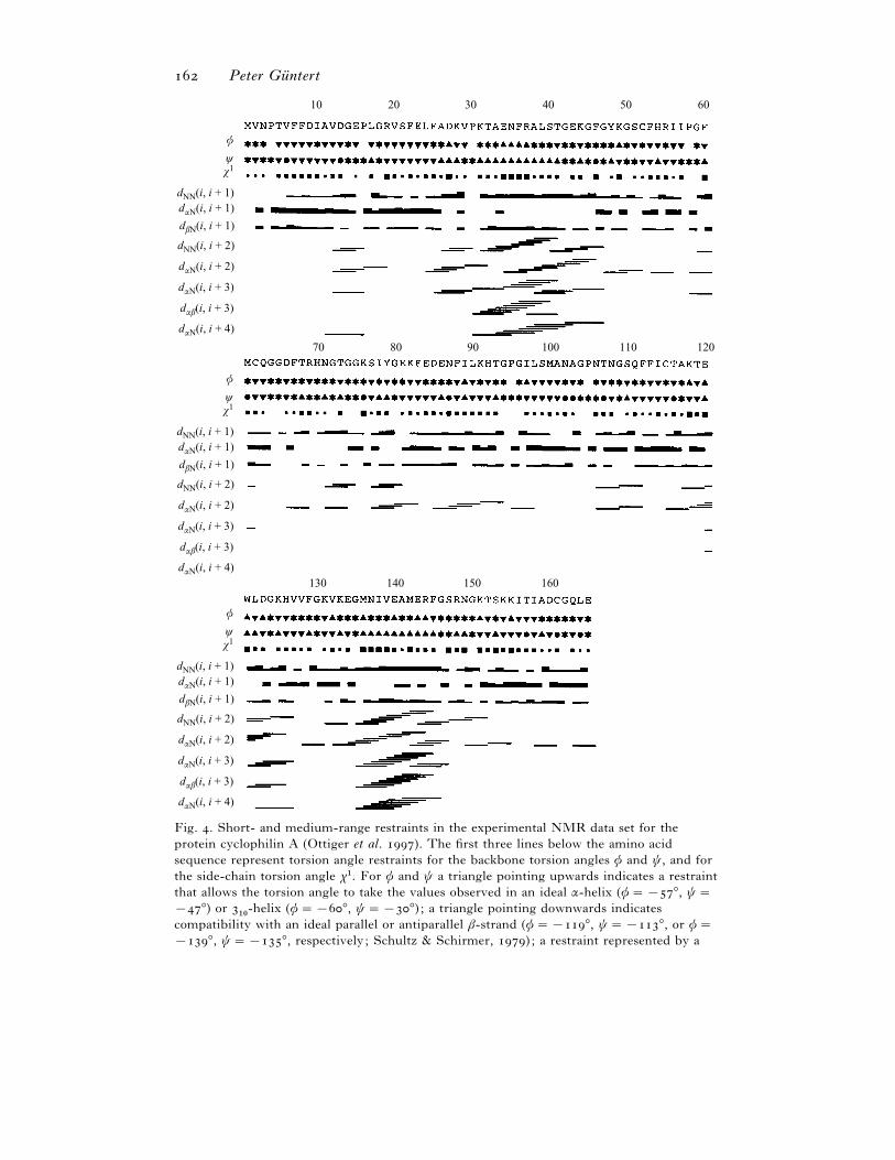
Fig. . Short- and medium-range restraints in the experimental NMR data set for the
protein cyclophilin A (Ottiger et al. ). The first three lines below the amino acid
sequence represent torsion angle restraints for the backbone torsion angles φ and ψ, and for
the side-chain torsion angle χ". For φ and ψ a triangle pointing upwards indicates a restraint
that allows the torsion angle to take the values observed in an ideal α-helix (φ¯®°, ψ¯®°) or
"!-helix (φ¯®°, ψ¯®°) ; a triangle pointing downwards indicates
compatibility with an ideal parallel or antiparallel β-strand (φ¯®°, ψ¯®°, or φ¯®°, ψ¯®°, respectively; Schultz & Schirmer, ) ; a restraint represented by a
Structure calculation of biological macromolecules
between the suppression of spin diffusion and sufficient cross peak intensities,
usually with mixing times in the range of – ms for high-quality structures.
Spin diffusion effects can be included in the structure calculation by complete
relaxation matrix refinement (Keepers & James, ; Yip & Case, ; Mertz
et al. ). Because also parameters about internal and overall motions that are
difficult to measure experimentally enter into the relaxation matrix refinement,
care has to be taken not to bias the structure determination by overinterpretation
of the data. Relaxation matrix refinement has been used mostly in situations where
the conservative and robust interpretation of NOEs as upper distance limits would
not be sufficient to define the three-dimensional structure, especially in the case of
nucleic acids (Wijmenga et al. ; Pardi, ; Varani et al. ).
The quantification of an NOE amounts to determining the volume of the
corresponding cross peak in the NOESY spectrum (Ernst et al. ). Since the
line-widths can vary appreciably for different resonances, cross peak volumes
should be determined by integration over the peak area rather than by measuring
peak heights, for example by counting contour lines. Integration is straightforward
for isolated cross peaks. For clusters of overlapping cross peaks deconvolution
methods have been proposed to distribute the total volume among the individual
signals (e.g. Denk et al. ; Koradi et al. ). While the reliable quantification
of NOEs is important to obtain a high-quality protein structure, one should also
keep in mind that, according to equation (), the relative error of the distance
estimate is only one sixth of the relative error of the volume determination.
On the basis of equation (), NOEs are usually treated as upper bounds on
interatomic distances rather than as precise distance restraints because the
presence of internal motions and, possibly, chemical exchange may diminish the
strength of an NOE (Ernst et al. ). In fact, much of the robustness of the
NMR structure determination method is due to the use of upper distance bounds
instead of exact distance restraints in conjunction with the observation that
internal motions and exchange effects usually reduce rather than increase the
NOEs (Wu$ thrich, ). For the same reason, the absence of a NOE is in general
not interpreted as a lower bound on the distance between the two interacting
spins. Certain NOEs, however, may also be enhanced by internal motions or
chemical exchange and then be incompatible with the assumption of a rigid
structure that fulfils all NMR data simultaneously (Torda et al. ;
Bru$ schweiler et al. ).
star encloses conformations of both α and β secondary structure types; and a filled circle
marks a restraint that excludes the torsion angle values of these regular secondary structure
elements. Torsion angle restraints for χ" are depicted by filled squares of three different
decreasing sizes, depending on whether they allow for none, one, two or all three of the
staggered rotamer positions χ"¯®, , °. Torsion angle restraints for χ" that exclude
all three staggered rotamer positions are shown as filled circles. Upper distance limits for
sequential and medium-range distances are shown by horizontal lines connecting the
positions of the two residues involved. The thickness of the lines for the sequential distances
dNN
(i, i), dαN(i, i) and dβN
(i, i) is inversely proportional to the squared upper
distance bound. The plot was produced with the program (Gu$ ntert et al. ).

Peter GuX ntert
Upper bounds u on the distance between two hydrogen atoms are derived from
the corresponding NOESY cross peak volumes V according to ‘calibration
curves’, V¯ f (u). Assuming a rigid molecule, the calibration curve is
V¯k
u'
()
with a constant k that depends on the arbitrary scaling of the NOESY spectrum.
The value u obtained from equation () may either be used directly as an upper
distance bound, or NOEs may be calibrated into different classes according to
their volume, using the same upper bound u for all NOEs in a given class. In this
case, it is customary to set the upper bound to ± AI for ‘strong’ NOEs, ± AI for
‘medium’ NOEs, and ± AI for ‘weak’ NOEs (Williamson et al. ; Clore et al.
b).
The constant k in equation can be determined on the basis of known distances,
for example the sequential distances d(Hα
i, HN
i+") and d(HN
i, HN
i+") in regular
secondary structure elements (Billeter et al. ), or by reference to a preliminary
structure (Gu$ ntert et al. b). Sometimes, especially in the course of an
automatic NOESY assignment procedure, it is convenient to get an estimate of k
independent from the knowledge of certain distances or preliminary structures.
This can be obtained, based on the observation that the average value ua of the
upper distance bounds u for NOEs among the backbone and β protons is similar
in all globular proteins, by setting k such that the average upper distance bound
becomes ua ¯ ± AI (Mumenthaler et al. ).
In practice, it has been observed that more conservative calibration curves, for
example of the type V¯ k}un, with n¯ or , may be advantageous for NOEs
with peripheral side-chain protons (Gu$ ntert et al. b). The uniform average
model (Braun et al. ) provides another, very conservative, calibration curve
by making the assumption that, due to internal motions, the interatomic distance,
r, assumes all values between the steric lower limit, l, and an upper limit, u, with
equal probability:
V¯k
u®l &u
l
dr
r'¯
k«u®l 0
l&®
u&1. ()
NOEs that involve groups of protons with degenerate chemical shifts, in
particular methyl groups, are commonly referred to pseudoatoms located in the
centre of the protons that they represent, and the upper bound is increased by a
pseudoatom correction equal to the proton–pseudoatom distance (Wu$ thrich et al.
).
Sometimes, especially in the case of nucleic acid structure determination, where
the standard, conservative interpretation of NOEs might not be sufficient to
obtain a well-defined structure, also lower distance limits have been attributed to
NOEs, either based on the intensity of the NOE or to reflect the absence of a
corresponding cross peak in the NOESY spectrum (Pardi, ; Varani et al.
). Such practices should be exercised with care because they may carry the
danger of overinterpretation of the experimental data and potentially jeopardize
the robustness of the NMR approach to structure determination.

Structure calculation of biological macromolecules
Fig. . Long-range distance restraints in the experimental NMR data set for the protein
cyclophilin A (Ottiger et al. ). Restraints between atoms five or more residues apart in
the sequence are represented by lines going from upper left to lower right (restraints
between side-chain atoms), or from lower left to upper right (restraints involving backbone
atoms). On the left and right hand sides the amino acid sequence of cyclophilin A is given.
Distance restraints can be visualized in a number of different ways. Short- and
medium-range restraints are best plotted against the sequence, as in Fig. which
was produced automatically by the program on the basis of the experimental
Peter GuX ntert
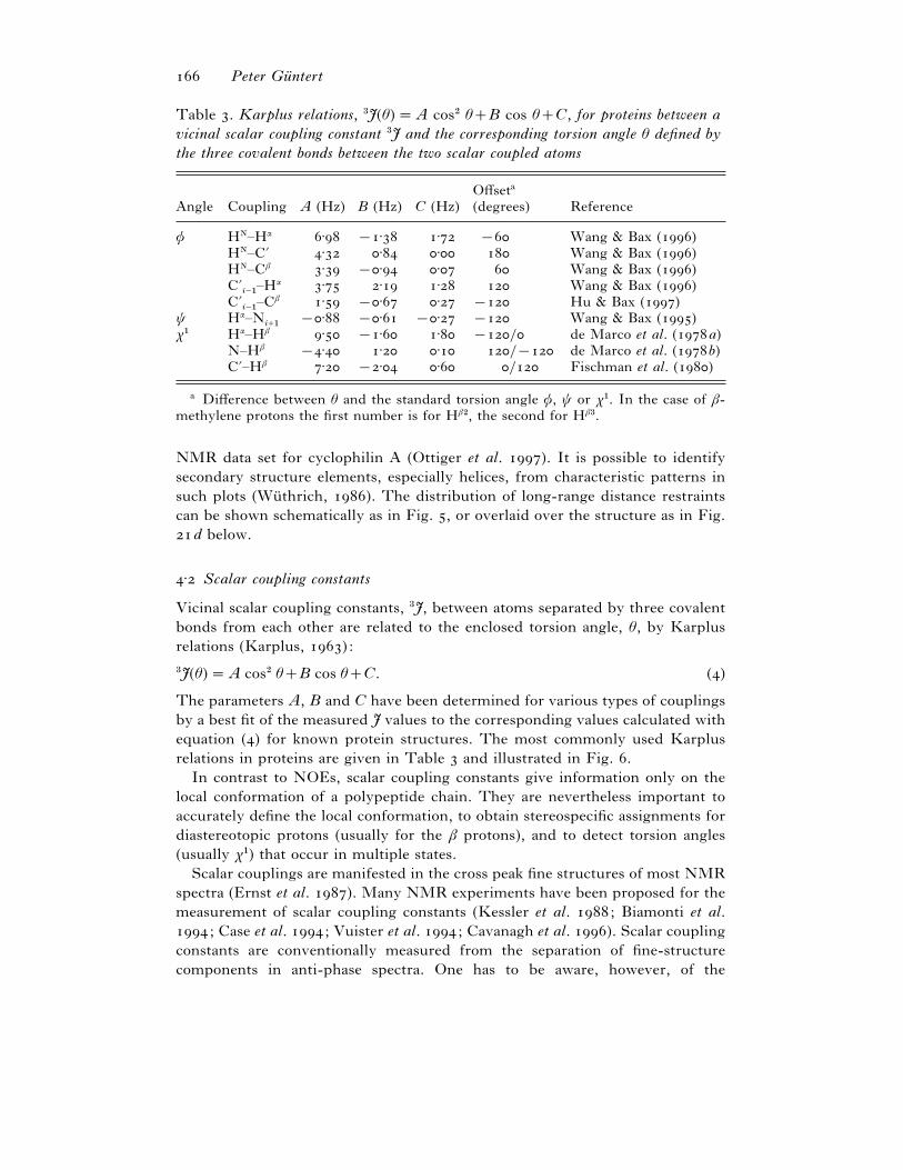
Table . Karplus relations, $J(θ)¯A cos# θB cos θC, for proteins between a
vicinal scalar coupling constant $J and the corresponding torsion angle θ defined by
the three covalent bonds between the two scalar coupled atoms
Angle Coupling A (Hz) B (Hz) C (Hz)
Offseta
(degrees) Reference
φ HN–Hα ± ®± ± ® Wang & Bax ()
HN–C« ± ± ± Wang & Bax ()
HN–Cβ ± ®± ± Wang & Bax ()
C«i−"
–Hα ± ± ± Wang & Bax ()
C«i−"
–Cβ ± ®± ± ® Hu & Bax ()
ψ Hα–Ni+"
®± ®± ®± ® Wang & Bax ()
χ" Hα–Hβ ± ®± ± ®} de Marco et al. (a)
N–Hβ ®± ± ± }® de Marco et al. (b)
C«–Hβ ± ®± ± } Fischman et al. ()
a Difference between θ and the standard torsion angle φ, ψ or χ". In the case of β-
methylene protons the first number is for Hβ#, the second for Hβ
$.
NMR data set for cyclophilin A (Ottiger et al. ). It is possible to identify
secondary structure elements, especially helices, from characteristic patterns in
such plots (Wu$ thrich, ). The distribution of long-range distance restraints
can be shown schematically as in Fig. , or overlaid over the structure as in Fig.
d below.
± Scalar coupling constants
Vicinal scalar coupling constants, $J, between atoms separated by three covalent
bonds from each other are related to the enclosed torsion angle, θ, by Karplus
relations (Karplus, ) :
$J(θ)¯A cos# θB cos θC. ()
The parameters A, B and C have been determined for various types of couplings
by a best fit of the measured J values to the corresponding values calculated with
equation () for known protein structures. The most commonly used Karplus
relations in proteins are given in Table and illustrated in Fig. .
In contrast to NOEs, scalar coupling constants give information only on the
local conformation of a polypeptide chain. They are nevertheless important to
accurately define the local conformation, to obtain stereospecific assignments for
diastereotopic protons (usually for the β protons), and to detect torsion angles
(usually χ") that occur in multiple states.
Scalar couplings are manifested in the cross peak fine structures of most NMR
spectra (Ernst et al. ). Many NMR experiments have been proposed for the
measurement of scalar coupling constants (Kessler et al. ; Biamonti et al.
; Case et al. ; Vuister et al. ; Cavanagh et al. ). Scalar coupling
constants are conventionally measured from the separation of fine-structure
components in anti-phase spectra. One has to be aware, however, of the

Structure calculation of biological macromolecules
JHN
Hα
JC′Hα
JHN
C′
JC′Cb
JHN
Cb
JHαN
JHαH
b2
JHαH
b3 JC′Hb3
JC′Hb2
JNHb3
JNHb2
8
4
0
0
2
12
8
4
0
–4
–180 –120 –60 0 60 120 180φ (°)
–180 –120 –60 0 60 120 180ψ (°)
–180 –120 –60 0 60 120 180χ1 (°)
3 J (
Hz)
3 J (
Hz)
3 J (
Hz)
Fig. . Karplus relations between vicinal scalar coupling constants and the torsion angles φ,
ψ and χ" in proteins. Karplus curves are drawn as solid lines for couplings between two
hydrogen atoms, as dotted lines for couplings between a carbon and a hydrogen atom, as
dot-dashed lines for couplings between two carbon atoms, and as dashed lines for couplings
between a nitrogen and a hydrogen atom. See also Table .
cancellation effects between positive and negative fine-structure elements that lead
both to an overestimation of the coupling constant and to a decrease of the overall
cross peak intensity (Neuhaus et al. ; Cavanagh et al. , pp. –).
These effects inhibit the determination of coupling constant values that are much
smaller than the line-width from anti-phase cross-peaks. The cancellation effects
can be reduced in E. COSY type spectra (Griesinger et al. ) where the cross
peak fine-structure is simplified by suppression of certain components of the
fine-structure. Other methods to determine coupling constants rely on the
measurement of cross peak intensity ratios (Vuister et al. ), on a series of
spectra with cross peak volumes modulated by the coupling constant (Neri et al.
), or on in-phase spectra (Szyperski et al. a). When interpreting scalar
coupling constants using equation () one has to take into account not only the
measurement error but also that there may be averaging due to internal mobility
and that both the functional form and the parameters of the Karplus curves are
approximations.

Peter GuX ntert
12
8
4
0
–4
–4 0 4 8 12
t
3JHαHb
g–
t
g+
g+
g–
3JC′Hb
3JNHb
g+t
3 J XH
b3 (
Hz)
3JXHb2 (Hz)
g–
Fig. . Relations between vicinal scalar coupling constants for β-methylene protons in
proteins. Solid and dotted lines correspond to the Karplus curves given in Table . Values
in the shaded areas result from additional mobility leading to χ" torsion angles that are
uniformly distributed within up to ³° around a given value. Ticks on the curves are set
in intervals of °, and the rotamer positions gauche (χ"¯°), gauche® (χ"¯®°) and
trans (χ"¯°) are labelled.
Motions that lead to fluctuations of θ about an average value reduce the
amplitude of the Karplus curve but do not strongly change the functional form.
For instance, if the torsion angle values are distributed uniformly in an interval
[θ®∆θ}, θ∆θ}] of width ∆θ centred at θ, the resulting Karplus curve
maintains the shape of equation () but with parameters A, B, C replaced by
A«¯Asin ∆θ
∆θ, B«¯B
sin∆θ
∆θ, C«¯C
A
0®sin ∆θ
∆θ 1. ()
In the case of uniform fluctuations of, say, the φ torsion angle of ³° around a
central value, this amounts to a maximal deviation of the Karplus curve given by
equations () from the corresponding one for a rigid molecule of ± Hz for
$JH
NH
α (Table ).
A different situation arises if the torsion angle fluctuates between distinctively
different conformations, for example if several rotamers of the χ" torsion angle are
populated. Under such conditions a direct interpretation of the measured J value
with equations () and () becomes meaningless. However, if several scalar
coupling constant values can be measured for a given torsion angle, the set of
values provides a method to detect whether the torsion angle is significantly
disordered because only certain combinations of the J values for different atom
pairs are compatible with a rigid structure (Fig. ).

Structure calculation of biological macromolecules
Sca
lar
coup
ling
con
stan
t
Torsion angle
Fig. . Conversion of scalar coupling constants to torsion angle restraints. Top: The shaded
range for the measured value of a scalar coupling constant leads, according to a Karplus
curve, to three separate allowed intervals of the corresponding torsion angle. Bottom: The
same allowed angle ranges, shown as sectors of a circle, and three torsion angle restraints,
represented by the inner concentric circles. Each restraint restricts the torsion angle to one
allowed interval. Applied simultaneously, the three restraints confine the torsion angle to
values that are in agreement with the measured coupling constant.
Torsion angle restraints in the form of an allowed interval are used to
incorporate scalar coupling information into the structure calculation. Using
equation (), an allowed range for a scalar coupling constant value in general leads
to several (up to four) allowed intervals for the enclosed torsion angle (Fig. ).
Restraining the torsion angle to a single interval that encloses all torsion angle
values compatible with the scalar coupling constant then often results in a loss of
structural information because the torsion angle restraint may encompass large
regions that are forbidden by the measured coupling constant. It is therefore often
advantageous to combine local data – for example all distance restraints and scalar
coupling constants within the molecular fragment defined by the torsion angles φ,
ψ, and χ" – in a systematic analysis of the local conformation and to derive torsion
angle restraints from the results of this grid search rather than from the individual
NMR parameters (see Section . below; Gu$ ntert et al. ).
Alternatively, scalar coupling constants can be introduced into the structure
calculation as direct restraints by adding a term of the type
VJ¯ k
J3i
($Jexpi
®$Jcalci
)# ()
to the target function of the structure calculation program (Kim & Prestegard,
; Torda et al. ). The sum in equation () extends over all measured

Peter GuX ntert
1·8 < dOH < 2·0 Å(a)
2·7 < dON < 3·0 Å
H
N
dOH < 2·4 Å(b)
α < 35°
ON
O
H
Fig. . (a) Hydrogen bond restraints used during a structure calculation (Williamson et al.
). (b) Criterion used to detect hydrogen bonds when analyzing a structure (Billeter et al.
; Koradi et al. ).
couplings, kJ
is a weighting factor, and $Jexpi
and $Jcalci
denote the experimental
and calculated value of the coupling constant, respectively. The latter is obtained
from the value of the corresponding torsion angle by virtue of equation ().
. Hydrogen bonds
Slow hydrogen exchange indicates that an amide proton is involved in a hydrogen
bond (Wagner & Wu$ thrich, ). Unfortunately, the acceptor oxygen or
nitrogen atom cannot be identified directly by NMR, and one has to rely on NOEs
in the vicinity of the postulated hydrogen bond or on assumptions about regular
secondary structure to define the acceptor. The standard backbone-backbone
hydrogen bonds in regular secondary structure can be identified with much higher
certainty than hydrogen bonds with side-chains. Hydrogen bond restraints are
thus either largely redundant with the NOE network or involve structural
assumptions, and should be used with care, or not at all. They can, however, be
useful during preliminary structure calculations of larger proteins when not
enough NOE data are available yet. Hydrogen bond restraints are introduced into
the structure calculation as distance restraints, typically by confining the acceptor-
hydrogen distance to the range ±–± AI and the distance between the acceptor
and the atom to which the hydrogen atom is covalently bound to ±–± AI (Fig.
a). The second distance restraint restricts the angle of the hydrogen bond. Being
tight medium- or long-range distance restraints, their impact on the resulting
structure is considerable. Restraints for architectural hydrogen bonds in secondary
structures enhance the regularity of the secondary structure elements. In fact,
helices and, to a lesser extent, β-sheets can be defined by hydrogen bond restraints
alone without the use of NOE restraints (Fig. ). On the other hand, hydrogen
bond restraints may lead, if assigned mechanically without clear-cut evidence, to
overly regular structures in which subtle features such as a "!
-helix-like final turn
of an α-helix may be missed.
. Chemical shifts
Chemical shifts are very sensitive probes of the molecular environment of a spin.
However, in many cases their dependence on the structure is complicated and
either not fully understood or too intricate to allow the derivation of reliable
conformational restraints (Oldfield, ; Williamson & Asakura, ). An
Structure calculation of biological macromolecules
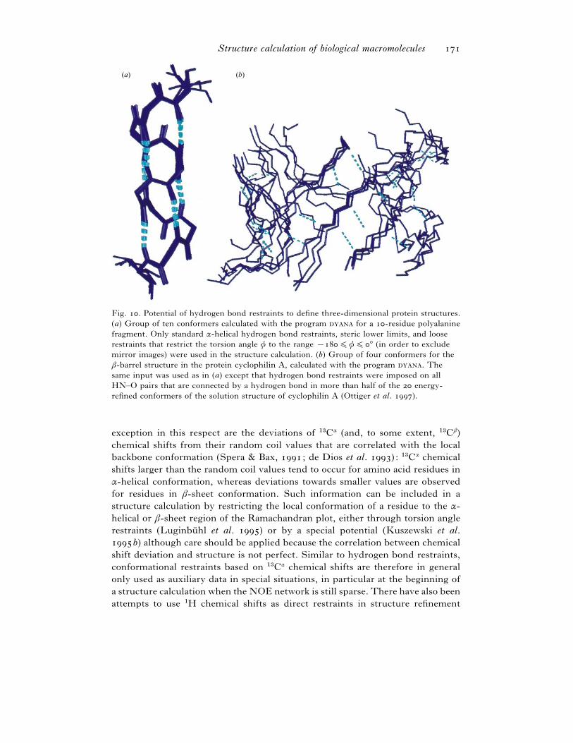
(a) (b)
Fig. . Potential of hydrogen bond restraints to define three-dimensional protein structures.
(a) Group of ten conformers calculated with the program for a -residue polyalanine
fragment. Only standard α-helical hydrogen bond restraints, steric lower limits, and loose
restraints that restrict the torsion angle φ to the range ®%φ%° (in order to exclude
mirror images) were used in the structure calculation. (b) Group of four conformers for the
β-barrel structure in the protein cyclophilin A, calculated with the program . The
same input was used as in (a) except that hydrogen bond restraints were imposed on all
HN–O pairs that are connected by a hydrogen bond in more than half of the energy-
refined conformers of the solution structure of cyclophilin A (Ottiger et al. ).
exception in this respect are the deviations of "$Cα (and, to some extent, "$Cβ)
chemical shifts from their random coil values that are correlated with the local
backbone conformation (Spera & Bax, ; de Dios et al. ) : "$Cα chemical
shifts larger than the random coil values tend to occur for amino acid residues in
α-helical conformation, whereas deviations towards smaller values are observed
for residues in β-sheet conformation. Such information can be included in a
structure calculation by restricting the local conformation of a residue to the α-
helical or β-sheet region of the Ramachandran plot, either through torsion angle
restraints (Luginbu$ hl et al. ) or by a special potential (Kuszewski et al.
b) although care should be applied because the correlation between chemical
shift deviation and structure is not perfect. Similar to hydrogen bond restraints,
conformational restraints based on "$Cα chemical shifts are therefore in general
only used as auxiliary data in special situations, in particular at the beginning of
a structure calculation when the NOE network is still sparse. There have also been
attempts to use "H chemical shifts as direct restraints in structure refinement

Peter GuX ntert
(O> sapay et al. ; Kuszewski et al. a). More often, however, they are used
to delineate secondary structure elements by virtue of the ‘chemical shift index’
(Wishart et al. ) or to assess the quality of a structure (Williamson et al. ).
. Residual dipolar couplings
Recently, a new class of conformational restraints has been introduced that
originates from residual dipolar couplings in partially aligned molecules and gives
information on angles between covalent bonds and globally defined axes in the
molecule, namely those of the magnetic susceptibility tensor (Tolman et al. ;
Tjandra et al. ). In contrast to vicinal scalar couplings or "$C secondary
chemical shifts that probe exclusively local features of the conformation, residual
dipolar couplings can provide information on long-range order which is not
directly accessible from other commonly used NMR parameters.
Residual dipolar couplings arise because the strong internuclear dipolar
couplings are no longer completely averaged out – as it is the case in a solution of
isotropically oriented molecules – if there is a small degree of molecular alignment
with the static magnetic field due to an anisotropy of the magnetic susceptibility.
The degree of alignment depends on the strength of the external magnetic field
and results in residual dipolar couplings that are proportional to the square of the
magnetic field strength (Gayathri et al. ). They are manifested in small, field-
dependent changes of the splitting normally caused by one-bond scalar couplings
between directly bound nuclei and can thus be obtained from accurate
measurements of "J couplings at different magnetic field strengths (Tolman et al.
; Tjandra et al. ). The magnetic susceptibility anisotropy is relatively
large in paramagnetic proteins (Tolman et al. ) but in general very small for
diamagnetic globular proteins. It can, however, be enhanced strongly if the
protein is brought into a liquid-crystalline environment (Losonczi & Prestegard,
; Tjandra & Bax, ).
Assuming an axially symmetric magnetic susceptibility tensor and neglecting
the very small contribution from ‘dynamic frequency shifts ’, the difference ∆Jobs
between the apparent J-values at two different magnetic field strengths, B(")
!and
B(#)
!, is given by (Tjandra et al. )
∆Jobs¯hγαγβχa
S
π#d$αβkB
T(B(#)
!®B(")
!)# ( cos# θ®), ()
where h is Planck’s constant, γα and γβ are the gyromagnetic ratios of the two spins
α and β, dαβ the distance between them, kB
the Boltzmann constant, T the
temperature, χa
the axial component of the magnetic susceptibility tensor, and S
the order parameter for internal motions (Lipari & Szabo, ). The structural
information is contained in the angle θ between the covalent bond connecting the
two scalar coupled atoms α and β and the main axis of the magnetic susceptibility
tensor; given all other constants, equation () yields an experimental value for
cos#θ. It is then straightforward to add an orientation restraint term to the target

Structure calculation of biological macromolecules
function of a structure calculation program that measures the deviation between
the value of cos#θobs obtained from equation () and the corresponding value
cos#θcalc calculated from the structure. Provided that the structure calculation
program allows free global reorientation of the molecule in space, the angle θcalc
can be measured simply with respect to an arbitrary fixed axis, for instance the z-
axis of the global coordinate system. The molecule will then rotate during the
structure calculation such as to align, under the simultaneous influence of all
orientation restraints, the main axis of the magnetic susceptibility tensor with the
z-axis. Tjandra et al. () have shown that such orientation restraints can be
used in conjunction with conventional distance and angle restraints during the
structure calculation, and that they can have a beneficial effect on the quality of the
resulting structure. Being in an early stage of their application, the potential of
orientation restraints in biomolecular structure calculation remains to be assessed
by further research. A particularly interesting, as yet unanswered question is
whether they will open an avenue towards non-NOE-based NMR structure
determination.
. Other sources of conformational restraints
Additional types of conformational restraints have been used occasionally in
NMR structure determination. These included, for example, ad hoc restraints to
enforce certain conformations that were believed to be present but could not be
found unambiguously on the basis of the ‘normal’ conformational restraints,
conformational database potentials to confine the structure to those regions of the
Ramachandran plot or side-chain conformation space that are populated in high-
resolution X-ray structures (Kuszewski et al. ), and restraints that are
available only for special systems. The latter include, for example, restraints
derived from pseudocontact shifts in paramagnetic proteins (Banci et al. ).
.
. Systematic analysis of local conformation
Due to the size and complexity of the conformation space of a biological
macromolecule, it is not possible to perform an exhaustive search that would yield
a complete description of the accessible regions in conformation space. However,
for limited fragments of the macromolecule exhaustive searches are feasible if
conformation space is discretized in the form of a multidimensional grid in which
each dimension corresponds to a torsion angle or to a group of dependent torsion
angles. The basic advantage of such ‘grid searches’ over statistical sampling
methods is that no conformations (on the grid) will be missed and that therefore
definite answers to questions like: ‘Are the local experimental data consistent with
a single rigid structure?’ can be given.
The role of grid searches in NMR structure calculation is three-fold: First,
inconsistencies among the experimental data can be detected. In general, a

Peter GuX ntert
significant fraction of the experimental restraints are short-range in nature and can
therefore be checked by considering limited fragments of the complete molecule.
Second, stereospecific assignments of diastereotopic protons or isopropyl groups
can be obtained by performing separate grid searches for both possible
stereospecific assignments (Gu$ ntert et al. ; Nilges et al. ; Polshakov et al.
). Third, experimental data such as scalar coupling constants and NOEs can
be converted into direct restraints on torsion angles that can be used by structure
calculation programs in order to improve both the precision of the resulting
structure and the success rate of the calculation.
Grid searches have been used most commonly to analyze the local conformation
of protein fragments involving the three torsion angles φ, ψ and χ" of an amino
acid residue, for example employing the programs (Gu$ ntert et al. ) or
(Nilges et al. ), with the aims of determining the stereospecific
assignment of the β-protons and obtaining restraints for the torsion angles φ, ψ
and χ" on the basis of intramolecular and sequential NOEs, and scalar coupling
constants within the fragment. Torsion angle restraints can be generated
regardless of whether or not an unambiguous stereospecific assignment for the β-
protons is obtained, simply by merging the results of the two grid searches for
both possible stereospecific assignments. Compared to manual, qualitative
conversions of scalar coupling constants into angle restraints (Wu$ thrich, )
and manually derived stereospecific assignments based on the assumption that the
χ" angle adopts only the three staggered rotamer positions, the automatic grid
search approach is more convenient and more objective. Grid search methods are
expected to be especially useful also in DNA}RNA structure determination,
because long-range NOEs are relatively scarce in nucleic acids and hence short-
range restraints become more important (Wijmenga et al. ; Pardi, ;
Varani et al. ).
A new grid search algorithm, implemented as a module of the D structure
calculation program (Gu$ ntert et al. ), extends the previous approach in
various directions (P. Gu$ ntert, M. Billeter, O. Ohlenschla$ ger, unpublished). It
can be applied in a straightforward manner as an automated step of a structure
calculation and is described here as an example of a versatile grid search algorithm.
In contrast to that was specific for φ, ψ and χ" fragments in proteins,
arbitrary fragments, defined as connected subsets of torsion angles in the
molecule, can be investigated. Covalent geometry parameters (bond lengths, bond
angles etc.) and Karplus curve relations (Table ) are stored in the standard
residue library. This allows the treatment of any type of molecule, in particular
proteins and nucleic acids. The fragment size is limited in practice only by the
computing power available. All upper and lower limit distance restraints, scalar
couplings and angle restraints available within the fragment are used. Criteria to
accept or reject conformations can be based either on the maximal restraint
violation in the fragment or on the local target function value (see below),
calculated for all restraints within the fragment. Stereospecific assignments can be
determined also for other groups than βCH#
and even if the fragment contains
more than one pair of diastereotopic substituents. Sets of dependent torsion angles

Structure calculation of biological macromolecules
are treated as a single degree of freedom. For example, the dependencies of the
ribose ring torsion angles ν!, ν
", ν
#, ν
$, ν
%on the pseudorotation angle P are given
by (Saenger, ) :
νk¯ ν
maxcos 0P
π
(k®)1 (P ` [,π] ; ν
max¯ °). ()
The parameter P is used as a single degree of freedom in the grid search. This
ensures that the relations among the dependent torsion angles are always fulfilled
and significantly increases the efficiency of the algorithm. Output torsion angle
restraints may comprise more than one allowed interval for one torsion angle (Fig.
). Results from different grid searches for overlapping fragments can be
combined, both in order to reduce the computational effort required for higher-
dimensional grid searches and in order to generate the narrowest possible output
torsion angle restraints.
The molecular fragment to be analysed in the grid search is defined by selecting
a connected subset of torsion angles (Fig. a). The program then extracts from
the data for the complete molecule the subset of conformational restraints within
the chosen fragment and evaluates them in a multidimensional grid search. The
grid search is implemented by n nested loops, each of which corresponds to a
degree of freedom. In routine applications the results of the grid search comprise
the number of allowed conformations, N, and the sets of allowed values for each
torsion angle in the fragment (Fig. b), i.e. information about correlations
between torsion angles is discarded. It is, however, possible to save all allowed
conformations for further analysis. The number of allowed conformations yields
the important information whether the set of restraints for a fragment is
compatible, within the given limits on the target function value or the sizes of
violations, with a rigid conformation (N" ) or not (N¯ ). Inconsistencies
among the local restraints can be detected in this way at the beginning of an NMR
structure determination. If the fragment under investigation contains M pairs of
diastereotopic substituents for which the stereospecific assignment is not known,
M grid searches will be performed, one for each combination of possible
stereospecific assignments, and their results will be combined. Alternatively, the
algorithm can be used also to find stereospecific assignments on the basis of local
restraints by checking whether the restraints are compatible with only one of the
two possible stereospecific assignment of a diastereotopic pair. In practice, a
complete local conformation analysis of a macromolecule includes many grid
searches for (possibly overlapping) fragments, and finally restraints are generated
for all torsion angles that formed part of at least one of the fragments.
. Stereospecific assignments
The standard method for obtaining resonance assignments in proteins (Wider et
al. ; Wu$ thrich et al. ) cannot provide stereospecific assignments, i.e.
individual assignments for the two diastereotopic substituents of a prochiral
centre, for example in methylene groups and in the isopropyl groups of valine and

Peter GuX ntert
(a)
(b)
Ser
Glu
Pro
–180 –150 –120 –90 –60 –30 0 30 60 90 120 150 180
28 ASN φv1
v2
w29 LEU φ
v1
v2
w
Fig. . (a) Ball-and-stick representation of a molecular fragment defined by the four torsion
angles φ, ψ, χ" and χ# (indicated by thick bonds) of the central Glu amino acid residue.
Atoms not included in the fragment are marked with ‘X’. (b) Allowed torsion angle ranges
(horizontal bars) obtained with the grid search module of the program for two φ-ψ-
χ"-χ#-fragments of the protein Pa, using the experimental NMR data set of Ferna!ndez et
al. ().
leucine. In the absence of stereospecific assignments restraints involving
diastereotopic substituents have to be referred to pseudoatoms (Wu$ thrich et al.
), or otherwise treated such that they are invariant under exchange of the two
diastereotopic substituents (see next section), which inevitably results in a loss of
information and less well defined structures (Gu$ ntert et al. ; Table below).
It is therefore important for obtaining a high-quality structure that as many
stereospecific assignments as possible are determined. Stereospecific assignments
of valine and leucine isopropyl groups can be determined experimentally by
biosynthetical fractional "$C-labelling (Senn et al. ; Neri et al. ).
Stereospecific assignments for methylene protons have to be determined in the
course of the structure calculation, either manually (Hyberts et al. ), by
systematic analysis of the local conformation around a methylene group, or by
reference to preliminary three-dimensional structures.

Structure calculation of biological macromolecules
The local method, introduced by Gu$ ntert et al. (), consists of two separate
grid searches, one for each of the two assignment possibilities. An unambiguous
stereospecific assignment results if allowed conformations occur only for one of
the two possible assignments. It relies exclusively on scalar coupling constants and
local distance restraints. Assuming realistic error ranges for experimental data it
will not be possible to obtain unambiguous stereospecific assignments by the local
method in all cases. Using complete simulated sets of local distance restraints and
homonuclear coupling constants with an accuracy of ³ Hz, it was estimated that
the program can yield unambiguous stereospecific assignments for about
% of the β-methylene protons (Gu$ ntert et al. ).
In contrast to the local method, global methods aim at the determination of
stereospecific assignments either during the calculation of a three-dimensional
structure or by reference to preliminary three-dimensional structures. They have
the potential advantage over the local method that all conformational restraints,
not only local ones, can be exploited, but, on the other hand, a systematic search
of allowed conformations is no longer feasible, and the stereospecific assignments
have to be based on a statistical analysis of a limited number of conformers. In
conjunction with structure calculation programs working in Cartesian coordinate
space, the so-called method of ‘floating stereospecific assignments’ (Weber et al.
) can be used: At the beginning of a structure calculation a strong reduction
of the corresponding potential energy terms allows the two diastereotopic
substituents to interchange freely under the influence of the restraints before they
later become fixed when the potential energy terms are slowly restored to their
normal values (which inhibit an interchange of the diastereotopic substituents). A
stereospecific assignment is considered to be unambiguous if it is found
consistently in all conformers that were calculated. Another simple method for
obtaining stereospecific assignments is implemented in the program of the
package (Gu$ ntert et al. a) and consists of an analysis of preliminary
three-dimensional structures: If there are two NOEs of significantly different
strength from a given proton to both diastereotopic substituents of a prochiral
centre and if the distances from the given proton to the two diastereotopic
substituents differ consistently in the structures, the stronger NOE can be
identified with the diastereotopic substituent that is closer to the given proton.
. Treatment of distance restraints to diastereotopic protons
Distance restraints involving diastereotopic substituents that could not be assigned
stereospecifically have to be modified such that they are invariant under exchange
of the two diastereotopic substituents. Traditionally, this is achieved by referring
the restraints to a pseudoatom located centrally with respect to the two
diastereotopic substituents and a concomitant increase of the upper distance
bound, bQ, by a pseudoatom correction, c
Q, equal to the distance from the
pseudoatom to the individual protons, i.e. bQ
¯min(b", b
#)c
Q, where b
"and b
#
are two individual upper bounds (Wu$ thrich et al. ). This approach, however,
completely discards the weaker of the two possible NOEs from a given proton to

Peter GuX ntert
the two diastereotopic substituents. Another straightforward method symmetrizes
the two restraints by imposing the less restrictive of the two upper bounds,
max (b", b
#), simultaneously on both distances to the individual diastereotopic
substituents. The pseudoatom and symmetrization treatments are not equivalent
and a combination of the two treatments, implemented in the programs
(Gu$ ntert et al. a) and (Gu$ ntert et al. ), can give improved results.
In addition, it makes use of the information from both upper bounds, b"
and b#,
also by assigning a more restrictive upper limit, bQ, to the restraint to the
pseudoatom,
bQ
¯b#"b#
#
®c#
Q. ()
Yet another approach, used for example in the program (Bru$ nger, ),
does not introduce a pseudoatom explicitly but assumes that the NOE originates
from both diastereotopic substituents simultaneously and imposes a distance
restraint on a ‘sum-averaged’ distance,
©dª¯ (d−'"
d−'#
)−"', ()
rather than on the individual distances to the two diastereotopic substituents, d"
and d#. Such sum-averaged distance restraints can be used for all groups of non-
stereoassigned or degenerate protons without the need for multiplicity or
pseudoatom corrections (Fletcher et al. ).
Fig. illustrates and compares the various methods in the two cases of
significantly different or similar upper bounds on the distances from the two
diastereotopic substituents to a third proton. Obviously, none of the methods can
completely make up for the loss of information that results from the absence of a
stereospecific assignment but there are significant differences between the various
procedures. In general, the loss of information is largest with the original
pseudoatom concept and smallest with the } treatment, which leads to
more precise structures (Gu$ ntert et al. a).
. Removal of irrelevant restraints
The number of experimental distance restraints used in a structure calculation is
an important parameter that determines the precision of the resulting structure.
To allow for meaningful comparisons it is therefore important to report the
number of relevant distance restraints, i.e. of those that actually restrict the
allowed conformation space, rather than the total number of NOESY cross peaks
that have been assigned. In addition, the removal of irrelevant distance restraints
increases slightly the efficiency of the structure calculation by obviating
unnecessary computations. In practice, often more than half of the intraresidual
and many sequential restraints are irrelevant. Those include restraints for fixed
distances, for example between geminal protons among the protons attached to an
aromatic ring, and distance bounds that cannot be reached by any conformation,
for example an upper bound of ± AI for the intraresidual distance between the

Structure calculation of biological macromolecules
2·8 Å4·2 Å
(a)
2·8 Å3·2 Å
2 Å2 ÅStereospecific
assignment
3·8 Å
(b)
3·8 Å
Pseudoatom
4·2 Å 4·2 Å(c)
3·2 Å3·2 Å
Symmetrization:Longer restraint
applied twice
3·43 Å (d)2·84 Å
Combination ofpseudoatom andsymmetrization
(e)
r–6 summation
Fig. . Treatment of distance restraints with diastereotopic protons. The situation of two
distance restraints of ± AI and ± AI (left column), or ± AI and ± AI (right column) from
two geminal methylene protons with a separation of AI to a common third atom is shown.
The methylene protons are shown as black dots, surrounded by white spheres with a radius
of AI that represent the sterically forbidden area around them. Dark shading indicates the
area of allowed positions for the third atom if the methylene protons are stereospecifically
assigned. Additionally allowed areas in the absence of a stereospecific assignment are shaded
in medium grey, and the individual distance restraints are shown as lightly shaded thin
circles. (a) Stereospecific assignment is available. (b) Conventional pseudoatom treatment
(Wu$ thrich et al. ). (c) The larger of the two upper distance bounds is applied to both
methylene protons. (d ) Combination of a pseudoatom treatment with minimal pseudoatom
correction and the method of two identical upper bounds as implemented in the programs
and . (e) The smaller of the two distance bounds is applied to the r−' sum of
the distances to the two methylene protons.

Peter GuX ntert
backbone amide- and the α-proton. Assuming rigid bond lengths and bond angles,
the latter condition can be checked readily for distances that depend on one or two
torsion angles (Gu$ ntert et al. a).
.
The calculation of the three-dimensional structure forms a cornerstone of the
NMR method for protein structure determination. Due to the complexity of the
problem – a protein typically consists of more than a thousand atoms which are
restrained by a similar number of experimentally determined restraints in
conjunction with stereochemical and steric conditions – it is in general neither
feasible to do an exhaustive search of allowed conformations nor to find solutions
by interactive model building. In practice, the calculation of the three-dimensional
structure is therefore usually formulated as a minimization problem for a target
function which measures the agreement between a conformation and the given set
of restraints. In the following, the four most widely used types of algorithms
(Table ) are discussed. Because the earlier methods have been reviewed
extensively already (Braun, ; Bru$ nger & Nilges, ; Sutcliffe, ; James,
; Nilges, ), special emphasis is given to the new structure calculation
method based on torsion angle dynamics which is currently the most efficient way
to calculate NMR structures of biological macromolecules.
± Metric matrix distance geometry
Distance geometry based on the metric matrix was the first approach used for the
structure calculation of proteins on the basis of NMR data (Braun et al. ;
Havel & Wu$ thrich, ). It relies on the fact that the NOE data and most of the
stereochemical data can be represented as distance restraints. Metric matrix
distance geometry is based on the theorem (Blumenthal, ; Crippen, ;
Crippen & Havel, ) that, given exact values for all distances among a set of
points in three-dimensional Euclidean space, it is possible to determine Cartesian
coordinates for these points uniquely except for a global inversion, translation and
rotation.
To see this, assume that all n¬n distances Dij¯ r r
i®r
jr are known among
n points in three-dimensional Euclidean space with (unknown) coordinates
r",… , r
nthat can be assumed, without loss of generality, to fulfill the relation
3iri¯ . Then, the n¬n metric matrix G, with elements
Gij¯ r
i[r
j¯
1
2
3
4
n3n
k="
D#ik®
n#3n
k, l="
D#kl, i¯ j
D#ij®G
ii®G
jj
, i1 j
()

Structure calculation of biological macromolecules
can be calculated. G has at most three positive eigenvalues λα with corresponding
n-dimensional eigenvectors eα that are related to the Cartesian coordinates
r",… , r
nof the n points by
rα
i¯oλα eα
i(α¯ , , ). ()
Equations () and () provide a straightforward way to embed a distance
matrix in three-dimensional space, i.e. to obtain Cartesian coordinates for a set of
points if all distances are known exactly. To make use of this theorem in a
structure calculation one has to account for the fact that in practice neither
complete nor exact distance information is available. Only for a small subset of all
distances dij, restraints in the form of lower and upper bounds, l
ij! d
ij! u
ij, can
be determined. Upper bounds result from NOEs, lower bounds from the steric
repulsion, and there are some exact distance constraints from known bond lengths
and bond angles of the covalent structure. To apply equations () and (),
unknown upper bounds are first initialized to a large value, and unknown lower
bounds to zero. Subsequently they are reduced by ‘bounds smoothing’ (Crippen,
), i.e. repeated application of the triangle inequality until all lower and upper
bounds are consistent with the triangle inequality. Then a complete set of
distances is produced by ‘randomly’ selecting for each distance a value between
the corresponding lower and upper bounds, and the embedding procedure
equations () and () is used to obtain Cartesian coordinates. Because the
assumptions of the embedding theorem are not met exactly, the resulting structure
will in general have the correct three-dimensional fold (or its mirror image) but
will be severely distorted. It needs to be regularized extensively, for example by
conjugate gradient minimization of an appropriate target function in Cartesian
coordinate space (Havel & Wu$ thrich, ). Nowadays a crudely regularized
structure is usually passed as start structure to simulated annealing by molecular
dynamics (Nilges et al. a ; Bru$ nger, ). Starting from the smoothed
distance bound matrix, the calculation is repeated with different ‘random’
selections of distances, in order to obtain a group of conformers whose spread
should give an indication of the allowed conformation space.
Despite the elegance of embedding method given by equations () and ()
there are a number of problems that have to be dealt with. Since all conformational
data has to be encoded into the distance matrix, it is not possible to introduce any
handedness or chirality. A structure and its mirror image are always equivalent for
metric matrix distance geometry. The correct handedness is only enforced during
regularization. For the same reason, torsion angle restraints cannot be used
directly in the embedding; they have to be represented by distance bounds,
thereby loosing part of their information.
The sampling of conformation space by a group of conformers resulting from
metric matrix distance geometry is decisively determined by the ‘random’
selection of distance values between corresponding lower and upper bounds. The
most straightforward method, namely selecting the distances as independent,
uniformly distributed random variables between the two limits, leads, because
meaningful upper bounds exist only for a small subset of all distances, on the

Peter GuX ntert
average to an overestimation of the true distances with the consequence of
artificially expanded structures (Metzler et al. ; Havel, ). This effect is
most pronounced in regions of the polypeptide chain for which only few restraints
are available. For example, chain ends that are unstructured in solution tend to be
forced into an extended conformation. A method to reduce – at the expense of
considerably increased computation time – such biased sampling of the allowed
conformation space is metrization (Havel & Wu$ thrich, ) : instead of selecting
the individual distances independently from each other, the bounds smoothing is
repeated each time after a distance value has been chosen, thereby resulting in a
more consistent set of distances for the embedding. This introduces, however, a
strong dependence of the sampling properties on the order in which the distances
are chosen (Havel, ). Good sampling can be achieved if the distances are
chosen in random order (Havel, , ). The computational efficiency of
metrization can be enhanced by partial metrization, i.e. by repeating the bounds
smoothing only after the selection of the first few percent of the randomly chosen
distances (Kuszewski et al. ).
. Variable target function method
The basic idea of the variable target function algorithm (Braun & Go, ) is to
gradually fit an initially randomized starting structure to the conformational
restraints collected with the use of NMR experiments, starting with intraresidual
restraints only, and increasing the ‘target size’ step-wise up to the length of the
complete polypeptide chain. Advantages of the method are its conceptual
simplicity and the fact that it works in torsion angle space, strictly preserving the
covalent geometry during the entire calculation. The variable target function
algorithm was implemented first in the program (Braun & Go, ) and
most commonly used in its implementation in the program (Gu$ ntert et al.
a), which is discussed here. Today, however, the variable target function
method has been superseded largely by the more efficient torsion angle dynamics
algorithm. Since both algorithms work in torsion angle space, they have many
features in common. These are described in detail in the section about torsion
angle dynamics below (see Section .).
The variable target function algorithm is based on the minimization of a target
function that includes terms for experimental and steric restraints. To reduce the
danger of becoming trapped in a local minimum with a function value much
higher than the global minimum, the target function is varied during a structure
calculation. At the outset only local restraints with respect to the polypeptide
sequence are considered. Subsequently, restraints between atoms further apart
with respect to the primary structure are included in a step-wise fashion (Fig. ).
Consequently, in the first stages of a structure calculation the local features of the
conformation will be established, and the global fold of the protein will be
obtained only towards the end of the calculation. The minimization algorithm
used in the program is the well-known method of conjugate gradients
(Powell, ) that tries to find the minimum by taking exclusively downhill steps.

Structure calculation of biological macromolecules
N Cα CCC′– – ––
–
Ri
N Cα CCC′– – –
–
Ri + 1
N Cα CCC′– – ––
–
N Cα CCC′– – –
–
Ri + 1Ri
N Cα CCC′– – –
Ri + 2
–
N Cα CCC′– – –
–
Ri
– N Cα CCC′– – ––
Ri – 1
NCαCCC′– ––
Rj
– NCαCCC′ – – –
–
Rj + 1
L = 0
L = 1
L = j – i
Fig. . Active restraints at various minimization levels L of the variable target function
algorithm. At a given minimization level L, all distance restraints between residues i and j
with r j®i r%L are considered.
As an alternative, a Newton–Raphson minimization algorithm that uses the matrix
of second derivatives (Abe et al. ) has been used in the program
(Endo et al. ).
A drawback of the basic implementation of the variable target function
algorithm (Braun & Go, ) is that for all but the simplest molecular topologies
only a small percentage of the calculations converge with small residual restraint
violations, which is a typical local minimum problem. Because of the low yield of
acceptable conformers, calculations had to be started with a large number of
randomized start conformers in order to obtain a group of good solutions,
sometimes compromising between the requirements of small restraint violations
and the available computing time (Kline et al. ). The introduction of the
optimized program (Gu$ ntert et al. a) reduced significantly the
computation time needed for the calculation of a single conformer, and a workable
situation was achieved for α-helical proteins (Gu$ ntert et al. b). Nonetheless,
the situation for β-proteins with more complex topology remained unsatisfactory
and was improved decisively only with the use of redundant dihedral angle
restraints ( ; Gu$ ntert & Wu$ thrich, ).
When using , the structure calculation is performed in iterative cycles that
provide a partial feedback of structural information gathered from the conformers
of the preceding cycle. To this end, an amino acid residue in a given conformer
is considered to have an acceptable conformation if the target function value due
to violations of restraints involving atoms or torsion angles of this residue is below
a predefined value, and if the same condition holds for the two sequentially
neighbouring residues, too. Redundant torsion angle restraints are then generated
and added to the input for the next cycle of structure calculations for all
Peter GuX ntert
residues that were found to be acceptable in a sufficient number of conformers by
taking the two extreme torsion angle values in the group of acceptable conformers
as upper and lower bounds. This method is able to reduce the computational effort
required to obtain a set of converged conformers by a factor of already in the
case of a small protein like BPTI. This improvement is achieved without
detectable reduction in the sampling of conformation space (Gu$ ntert & Wu$ thrich,
). To rationalize the empirically found higher yield of good conformers with
the use of it is important to note that in many regions of a protein structure,
in particular in β-strands, the local conformation is determined not only by the
local conformational restraints, but also by long-range restraints, such as
interstrand distance restraints in β-sheets. The local restraints alone may allow for
multiple local conformations at low target levels in a variable target function
calculation, of which some may be incompatible with the long-range restraints
taken into account later during the calculation. Obviously, incorrect local
conformations that satisfy the experimentally available local restraints are potential
local minima that could only be ruled out from the beginning if the information
contained in the long-range restraints were already available at low levels of the
minimization. The use of achieves this : information contained in the
complete data set is translated into (by definition intraresidual) torsion angle
restraints. It further makes clear why the yield of good solutions with the original
variable target function method (Braun & Go, ) was in general higher for α-
proteins than for β-proteins, since the conformation of an α-helix is particularly
well-determined by sequential and medium-range restraints.
. Molecular dynamics in Cartesian space
This third major method for NMR structure calculation is based on numerically
solving Newton’s equation of motion in order to obtain a trajectory for the
molecular system (Allen & Tildesley, ). The degrees of freedom are the
Cartesian coordinates of the atoms. In contrast to ‘standard’ molecular dynamics
simulations (McCammon & Harvey, ; Brooks et al. ; van Gunsteren &
Berendsen, ) that try to simulate the behaviour of a real physical system as
closely as possible (and do not include restraints derived from NMR), the purpose
of a molecular dynamics calculation in an NMR structure determination is simply
to search the conformation space of the protein for structures that fulfil the
restraints, i.e. that minimize a target function which is taken as the potential
energy of the system. Therefore, simulated annealing (Kirkpatrick et al. ;
Nilges et al. a ; Scheek et al. ; Bru$ nger & Nilges, , Bru$ nger et al.
) is performed at high temperature using a simplified force field that treats the
atoms as soft spheres without attractive or long-range (i.e. electrostatic) non-
bonded interactions, and that does not include explicit consideration of the
solvent. The distinctive feature of molecular dynamics simulation when compared
to the straightforward minimization of a target function is the presence of kinetic
energy that allows to cross barriers of the potential surface, thereby reducing
greatly the problem of becoming trapped in local minima. Since molecular

Structure calculation of biological macromolecules
dynamics simulation cannot generate conformations from scratch, a start structure
is needed, that can be generated either by metric matrix distance geometry (Nilges
et al. a) or by the variable target function method, but – at the expense of
increased computation time – it is also possible to start from an extended structure
(Nilges et al. c) or even from a set of atoms randomly distributed in space
(Nilges et al. b). Any general molecular dynamics program, such as
(Brooks et al. ), (Pearlman et al. ), or (van Gunsteren et
al. ), can be used for the simulated annealing of NMR structures, provided
that pseudoenergy terms for distance and torsion angle restraints have been
incorporated. In practice, the program best adapted and most widely used for this
purpose is (Bru$ nger, ).
The classical dynamics of a system of n particles with masses miand positions
riis governed by Newton’s equation of motion,
mi
d#ri
dt#¯F
i(i¯ ,… , n), ()
where the forces Fi
are given by the negative gradient of the potential energy
function Epot
with respect to the Cartesian coordinates: Fi¯®~
iE
pot. For
simulated annealing a simplified potential energy function is used that includes
terms to maintain the covalent geometry of the structure by means of harmonic
bond length and bond angle potentials, torsion angle potentials, terms to enforce
the proper chiralities and planarities, a simple repulsive potential instead of the
Lennard-Jones and electrostatic non-bonded interactions, as well as terms for
distance and torsion angle restraints. For example, in the program
(Bru$ nger, ),
E¯ 3bonds
kb(r®r
!)# 3
angles
kθ(θ®θ!)# 3
dihedrals
kφ(cos (nφδ))
3impropers
kφ(φ®δ)# 3nonbonded
pairs
krepel
(max (, (sRmin
)#®R#))#
3distancerestraints
kd∆#
d 3
anglerestraints
ka∆#
a()
kb, kθ, kφ, k
repel, k
dand k
adenote the various force constants, r the actual and r
!
the correct bond length, respectively, θ the actual and θ!and correct bond angle,
φ the actual torsion angle or improper angle value, n the number of minima of the
torsion angle potential, δ an offset of the torsion angle and improper potentials,
Rmin
the distance where the van der Waals potential has its minimum, R the actual
distance between a non-bonded atom pair, s a scaling factor, and ∆dand ∆
athe size
of the distance or torsion angle restraint violation. As an alternative to the square-
well potential of equation (), distance restraints are often represented by a
potential with linear asymptote for large violations (Bru$ nger, ). To obtain a
trajectory, the equations of motion are numerically integrated by advancing the
coordinates riand velocities v
i¯ rd
iof the particles by a small but finite time step
Peter GuX ntert
∆t, for example according to the ‘ leap-frog’ integration scheme (Hockney, ;
Allen & Tildesley, ) :
vi(t∆t})¯ v
i(t®∆t})∆t F
i(t)}m
iO(∆t$), ()
ri(t∆t)¯ r
i(t)∆t v
i(t∆t})O(∆t$). ()
The O(∆t$) terms indicate that the errors with respect to the exact solution
incurred by the use of a finite time step ∆t are proportional to ∆t$. The time step
∆t must be small enough to sample adequately the fastest motions, i.e. of the order
of −"& s. In general the highest frequency motions are bond length oscillations.
Therefore, the time step can be increased if the bond lengths are constrained to
their correct values by the method (Ryckaert et al. ). The temperature
may be controlled by coupling the system loosely to a heat bath (Berendsen et al.
). For the simulated annealing of a (possibly distorted) start structure, certain
measures have to be taken in order to achieve sampling of the conformation space
within reasonable time (Nilges et al. a). In a typical simulated annealing
protocol (Bru$ nger, ), the simulated annealing is performed for a few
picoseconds at high temperature, say T¯ K, starting with a very small
weight for the steric repulsion that allows atoms to penetrate each other, and
gradually increasing the strength of the steric repulsion during the calculation.
Subsequently, the system is cooled down slowly for another few picoseconds and
finally energy-minimized. This process is repeated for each of the start conformers.
The alternative of selecting conformers that represent the solution structure at
regular intervals from a single trajectory is used rarely because it is difficult to
judge whether the spacing between the ‘snapshots ’ is sufficient for good sampling
of conformation space. In general, simulated annealing by molecular dynamics
requires substantially more computation time per conformer (Bru$ nger, )
than, for example, the variable target function method but this effect may be
compensated by a higher success rate of –% of the start conformers which
is due to the ability of the algorithm to escape from local minima.
. Torsion angle dynamics
Torsion angle dynamics, i.e. molecular dynamics simulation using torsion angles
instead of Cartesian coordinates as degrees of freedom (Bae & Haug, ;
Gu$ ntert et al. ; Jain et al. ; Katz et al. ; Kneller & Hinsen, ;
Mathiowetz et al. ; Mazur & Abagyan, ; Mazur et al. ; Rice &
Bru$ nger, ; Stein et al. ), provides at present the most efficient way to
calculate NMR structures of biomacromolecules. In this section the torsion angle
dynamics algorithm implemented in the program (Gu$ ntert et al. ) is
described in some detail. This seems warranted in light of the wide-spread but
incorrect belief that dynamics in generalized coordinates is hopelessly complicated
and cannot be done efficiently. employs the torsion angle dynamics
algorithm of Jain et al. () that requires a computational effort proportional to
the system size, as it is the case for molecular dynamics simulation in Cartesian

Structure calculation of biological macromolecules
Table . Comparison of molecular dynamics simulation in Cartesian and torsion
angle space
Quantity Cartesian space Torsion angle space
Degrees of
freedom
N coordinates:
x", … , x
N
n torsion angles:
θ", … , θ
n
Equations Newton’s equations: Lagrange equations:
of motionm
ixXi¯®
¥Epot
¥xi
d
dt 0¥L
¥θdk
1®¥L
¥θk
¯ (L¯Ekin
®Epot
)
Kinetic energy Ekin
¯
3N
i="
mixd #i
Ekin
¯
3n
k, l="
M(θ)klθdkθdl
Mass matrix M Diagonal, elements mi
n¬n, non-diagonal, non-constant
Accelerations xXi¯®
mi
¥Epot
¥xi
θX ¯M(θ)−" C(θ, θd ) (n linear equations)
Computational
complexity of
acceleration
calculation
Proportional to N If solving system of linear equations:
proportional to n$
If exploiting tree structure of molecule:
proportional to n
space, too. The advantages of torsion angle dynamics, especially the much longer
integration time steps that can be used, are therefore effective for molecules of all
sizes, and in particular for large biological macromolecules. A comparison of
molecular dynamics simulation in Cartesian and torsion angle space in Table
shows the close analogy between the two methods.
.. Tree structure of the molecule
For torsion angle dynamics calculations with the molecule is represented
as a tree structure consisting of a base rigid body that is fixed in space and n rigid
bodies, which are connected by n rotatable bonds (Fig. a ; Katz et al. ; Abe
et al. ). The degrees of freedom are exclusively torsion angles, i.e. rotations
about single bonds. Each rigid body is made up of one or several mass points
(atoms) with invariable relative positions. The tree structure starts from a ‘base’,
typically at the N-terminus of the polypeptide chain, and terminates with ‘ leaves’
at the ends of the side-chains and at the C-terminus. The rigid bodies are
numbered from to n. The base has the number . Each other rigid body, with
a number k& , has a single nearest neighbour in the direction toward the base,
which has a number p(k)! k (Fig. ). The torsion angle between the rigid bodies
p(k) and k is denoted by θk. The conformation of the molecule is uniquely
specified by the values of all torsion angles, θ¯ (θ",… , θ
n). For each rotatable
bond, ek
denotes a unit vector in the direction of the bond, and rk
is the position
vector of its end point, which is subsequently used as the ‘reference point ’ of the
rigid body k. In the following description these and all other three-dimensional
vectors are referred to an inertial frame of reference that is fixed in space. Covalent

Peter GuX ntert
(a)
(b)
φ w φ w φ w
v1 v1 v1
v21 v22 v2 v21 v22
v3
Angular velocity xk
Linear velocity vkRigid body k(mass mk, inertia tensor lk)
Centre of massYk
Referencepoint rk
hkTorsionangle
ek
Rigid body p(k)
Fig. . (a) Tree structure of torsion angles for the tripeptide Val–Ser–Ile. Circles represent
rigid units. Rotatable bonds are indicated by arrows that point towards the part of the
structure that is rotated if the corresponding dihedral angle is changed. (b) Excerpt from the
tree structure formed by the torsion angles of a molecule, and various quantities required by
the torsion angle dynamics algorithm of Jain et al. ().
bonds that are incompatible with a tree structure because they would introduce
closed flexible rings, for example disulphide bridges, are treated, as in Cartesian
space dynamics, by distance constraints.
.. Potential energy
The target function V takes the role of the potential energy Epot
, i.e. Epot
¯w!V,
with an overall weighting factor w!¯ kJ mol−"AI −#. The target function V&
is defined such that V¯ if and only if all experimental distance restraints and
torsion angle restraints are fulfilled and all non-bonded atom pairs satisfy a
check for the absence of steric overlap. It measures restraint violations such that
V(θ)!V(θ«) whenever a conformation θ satisfies the restraints more closely than
another conformation θ«. The exact definition of the target function is :
V¯ 3c=u, l,v
wc
3(α,β) `Ic
fc(dαβ, bαβ)w
a3
i `Ia
0®
0∆
i
Γi
1#1∆#
"()

Structure calculation of biological macromolecules
Upper and lower bounds, bαβ, on distances between two atoms α and β, dαβ, and
restraints on individual torsion angles θi
in the form of allowed intervals,
[θmini
, θmaxi
], are considered. Iu, I
land I
vare the sets of atom pairs (α, β) with
upper, lower or van der Waals distance bounds, respectively, and Ia
is the set of
restrained torsion angles. wu, w
l, w
vand w
aare weighting factors for the different
types of restraints. Γi¯π®(θmax
i®θmin
i)} denotes the half-width of the forbidden
range of torsion angle values, and ∆i
is the size of the torsion angle restraint
violation. The target function of equation () is continuously differentiable over
the entire conformation space, and is chosen such that the contribution of a single
small violation δcis given by w
cδ#cfor all types of restraints. The sets I
u, I
land I
v
of distance restraints that contribute to the target function can include all distance
restraints or only those between residues with sequence numbers that differ by not
more than a given target level L (Fig. ).
The function fc(d, b) that measures the contribution of a violated distance
restraint to the target function can be a simple square potential,
fc(d, b)¯ (d®b)#, ()
or have the form used in the program (Gu$ ntert et al. a),
fc(d, b)¯ 0d#®b#
b 1#, ()
or be a function with a linear asymptote for large restraint violations
fc(d, b)¯ β#b# 9 0d®b
βb 1#
®:, ()
where β is a dimensionless parameter that weighs large violations relative to small
ones. For small restraint violations equations ()–() all yield the same
contribution, which is always equal to the square of the restraint violation, but
there is a pronounced difference for large violations, where the contributions are
proportional to the second, fourth and first power of the restraint violation,
respectively (Fig. ).
The torques about the rotatable bonds, i.e. the negative gradients of the
potential energy with respect to torsion angles, ®~Epot
, are calculated by the fast
recursive algorithm of Abe et al. (). The partial derivative of the function V
of equation () with respect to a torsion angle θk
is given by
¦V
¦θk
¯®ek[g
k®(e
kgr
k)[h
kw
a3
i `Ia
0®0∆i
Γi
1#1∆iδik, ()
where
gk¯ 3
c=u, l,v
wc
3(α,β) `Icα `Mk
¦fc(dαβ, bαβ)
¦dαβ
rαgrβ
dαβ
,
hk¯ 3
c=u, l,v
wc
3(α,β) `Icα `Mk
¦fc(dαβ, bαβ)
¦dαβ
rα®rβ
dαβ
.
5
6
7
8
()
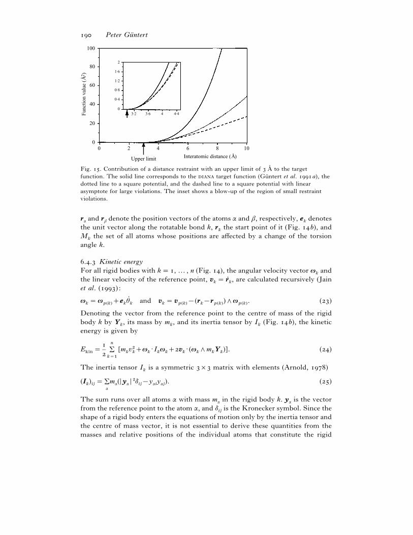
Peter GuX ntert
100
80
60
40
20
00 2 4 6 8 10
Upper limit Interatomic distance (Å)
Fun
ctio
n va
lue
(Å2 )
2
1·6
1·2
0·8
0·4
03·2 3·6 4 4·4
Fig. . Contribution of a distance restraint with an upper limit of AI to the target
function. The solid line corresponds to the target function (Gu$ ntert et al. a), the
dotted line to a square potential, and the dashed line to a square potential with linear
asymptote for large violations. The inset shows a blow-up of the region of small restraint
violations.
rα and rβ denote the position vectors of the atoms α and β, respectively, ekdenotes
the unit vector along the rotatable bond k, rk
the start point of it (Fig. b), and
Mk
the set of all atoms whose positions are affected by a change of the torsion
angle k.
.. Kinetic energy
For all rigid bodies with k¯ , … , n (Fig. ), the angular velocity vector ωk
and
the linear velocity of the reference point, vk¯ rd
k, are calculated recursively (Jain
et al. () :
ωk¯ω
p(k)e
kθdk
and vk¯ v
p(k)®(r
k®r
p(k))gω
p(k). ()
Denoting the vector from the reference point to the centre of mass of the rigid
body k by Yk, its mass by m
k, and its inertia tensor by I
k(Fig. b), the kinetic
energy is given by
Ekin
¯
3n
k="
[mkv#kω
k[I
kω
kv
k[(ω
kgm
kY
k)]. ()
The inertia tensor Ik
is a symmetric ¬ matrix with elements (Arnold, )
(Ik)ij¯3
α
mα(ryα r #δij®yαi
yαj). ()
The sum runs over all atoms α with mass mα in the rigid body k. yα is the vector
from the reference point to the atom α, and δij
is the Kronecker symbol. Since the
shape of a rigid body enters the equations of motion only by the inertia tensor and
the centre of mass vector, it is not essential to derive these quantities from the
masses and relative positions of the individual atoms that constitute the rigid

Structure calculation of biological macromolecules
body, as in equation (). In fact, the efficiency of the torsion angle dynamics
algorithm can be improved by treating the rigid bodies as solid spheres of mass mk
and radius ρ centred at the reference points rk:
Yk¯ and I
k¯ #
&m
kρ#
$, ()
where $is the ¬ unit matrix. In ρ¯ AI and m
k¯ on
km
!are used,
where nk
denotes the number of atoms in the rigid body k (not counting
pseudoatoms), and m!¯ ±¬−#( kg is the atomic mass unit. In this way, fast
motions of light rigid bodies, for example hydroxyl protons, are slowed down,
thereby permitting longer integration time steps. Equation () does not imply an
approximation of the van der Waals interaction: the steric repulsion is still
calculated for each individual atom pair.
.. Torsional accelerations
The calculation of the torsional accelerations, i.e. the second time derivatives of
the torsion angles, is the crucial point of a torsion angle dynamics algorithm. The
equations of motion for a classical mechanical system with generalized coordinates
are the Lagrange equations
d
dt 0¦L
¦θdk
1®¦L
¦θk
¯ (k¯ , … , n), ()
with the Lagrange function L¯Ekin
®Epot
(Arnold, ). They lead to
equations of motion of the form
M(θ)θX C(θ, θd )¯ . ()
In the case of torsion angles as degrees of freedom, the n¬n mass matrix M(θ) and
the n-dimensional vector C(θ, θd ) can be calculated explicitly (Mazur & Abagyan,
; Mazur et al. ). However, to integrate the equations of motion, equation
() would have to be solved in each time step for the torsional accelerations, θX .This requires the solution of a system of n linear equations and hence entails a
computational effort proportional to n$ that would become prohibitively expensive
for larger systems. Therefore, in the fast recursive algorithm of Jain et al.
() is implemented to compute the torsional accelerations, which makes
explicit use of the aforementioned tree structure of the molecule in order to obtain
θ$ with a computational effort that is only proportional to n.
The algorithm of Jain et al. () is initialized by calculating for all rigid
bodies, k¯ , … , n, the six-dimensional vectors
ak¯ 9 (ω
kge
k)θd
k
ωp(k)
g(vk®v
p(k)):, e
k¯ 9ek
: and zk¯ 9 ω
kgI
kω
k
(ωk\m
kY
k)ω
k®ω#
km
kY
k
:, ()
and the ¬ matrices
Pk¯ 9 I
k
®mkA(Y
k)
mkA(Y
k)
mk$
: and φk¯ 9$
$
A(rk®r
p(k))
$
:. ()
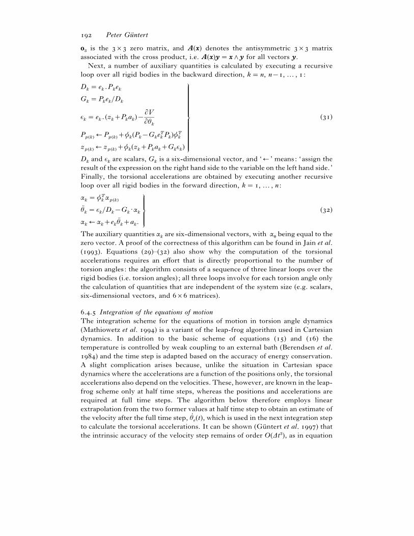
Peter GuX ntert
$
is the ¬ zero matrix, and A(x) denotes the antisymmetric ¬ matrix
associated with the cross product, i.e. A(x)y¯ xgy for all vectors y.
Next, a number of auxiliary quantities is calculated by executing a recursive
loop over all rigid bodies in the backward direction, k¯ n, n®, … , :
Dk¯ e
k\P
kek
Gk¯P
kek}D
k
εk¯ e
k\(z
kP
kak)®
¦V
¦θk
Pp(k)
"Pp(k)
φk(P
k®G
keTkPk)φT
k
zp(k)
" zp(k)
φk(z
kP
kakG
kεk)
5
6
7
8
()
Dk
and εk
are scalars, Gk
is a six-dimensional vector, and ‘" ’ means: ‘assign the
result of the expression on the right hand side to the variable on the left hand side. ’
Finally, the torsional accelerations are obtained by executing another recursive
loop over all rigid bodies in the forward direction, k¯ , … , n :
αk¯φT
kαp(k)
θXk¯ ε
k}D
k®G
k[α
k
αk"α
ke
kθXka
k.
5
6
7
8
()
The auxiliary quantities αkare six-dimensional vectors, with α
!being equal to the
zero vector. A proof of the correctness of this algorithm can be found in Jain et al.
(). Equations ()–() also show why the computation of the torsional
accelerations requires an effort that is directly proportional to the number of
torsion angles: the algorithm consists of a sequence of three linear loops over the
rigid bodies (i.e. torsion angles) ; all three loops involve for each torsion angle only
the calculation of quantities that are independent of the system size (e.g. scalars,
six-dimensional vectors, and ¬ matrices).
.. Integration of the equations of motion
The integration scheme for the equations of motion in torsion angle dynamics
(Mathiowetz et al. ) is a variant of the leap-frog algorithm used in Cartesian
dynamics. In addition to the basic scheme of equations () and () the
temperature is controlled by weak coupling to an external bath (Berendsen et al.
) and the time step is adapted based on the accuracy of energy conservation.
A slight complication arises because, unlike the situation in Cartesian space
dynamics where the accelerations are a function of the positions only, the torsional
accelerations also depend on the velocities. These, however, are known in the leap-
frog scheme only at half time steps, whereas the positions and accelerations are
required at full time steps. The algorithm below therefore employs linear
extrapolation from the two former values at half time step to obtain an estimate of
the velocity after the full time step, θde(t), which is used in the next integration step
to calculate the torsional accelerations. It can be shown (Gu$ ntert et al. ) that
the intrinsic accuracy of the velocity step remains of order O(∆t$), as in equation

Structure calculation of biological macromolecules
(). A time step t! t∆t that follows a preceding time step t®∆t«! t is executed
as follows:
. On the basis of the torsional positions θ(t), calculate the Cartesian coordinates
of all atoms (Katz et al. ; Gu$ ntert, ), the potential energy Epot
(t)¯E
pot(θ(t)), and the torques ®~E
pot(t).
. Adapt the torsional velocities θd (both θd (t®∆t«}) and θde(t)) to maintain the
temperature T ref (Berendsen et al. ) and adjust the time step to attain a
desired relative accuracy of energy conservation εref :
θd ¯ θd « T ref®T(t)
τT(t)and ∆t¯∆t«
εref®ε(t)
τε(t), ()
where
T(t)¯E
kin(t)
nkB
and ε(t)¯ )E(t)®E(t®∆t«)E(t) ), ()
respectively, are the instantaneous temperature and the relative change of the total
energy, E¯Ekin
Epot
, in the preceding time step. The time constant, τ( , is a
user-defined parameter, measured in units of the time step, with a typical value of
τ¯ ; n denotes the number of torsion angles and kB
¯ ±¬−#$J K−" is the
Boltzmann constant. Temperature and time step control can be turned off by
setting τ¯¢. To calculate ε(t) in equation (), E(t) is evaluated before velocity
scaling is applied, whereas for E(t®∆t«) the value after velocity scaling in the
preceding time step is used. Thus, the measurement of the accuracy of energy
conservation is not affected by the scaling of velocities. An exact algorithm would
yield E(t)¯E(t®∆t«) and consequently ε(t)¯ .
. Calculate the torsional accelerations, θX (t)¯ θX (θ(t),θde(t)), using equations
()–().
. Using the leap-frog scheme of equations () and () (with r replaced by θ),
calculate the new velocities at half time step, θd (t∆t}), and the new torsional
positions θ(t∆t).
The algorithm is initialized by setting t¯ , ∆t«¯∆t, and the initial torsional
velocities are chosen randomly corresponding to a given initial temperature.
Since for optimal efficiency in structure calculations with torsion angle dynamics
the time steps are made as long as possible a safeguard against occasional strong
violations of energy conservation by more than % in a single time step replaces
such time steps by two time steps of half length.
.. Energy conservation and time step length
Energy conservation is a key feature of proper functioning of any molecular
dynamics algorithm (Allen & Tildesley, ). The accuracy of energy
conservation can be monitored by the standard deviation σE
¯o©(E®©Eª)#ª,
or by the RMS change of the total energy between successive integration steps,
δE
¯o©∆E#ª, where ©…ª denotes the average over all time steps of a molecular
dynamics run (Beeman, ; van Gunsteren & Berendsen, ). The parameter
δE
is closely related to ε(t) in equation () and probes the local error in one time

Peter GuX ntert
step of the integration algorithm, whereas the standard deviation δE
is sensitive
both to local errors and to slow drifts of the total energy over many time steps and
is thus dependent on the length of molecular dynamics run. The dependence of
σE
and δE
on the length of the integration time step ∆t is plotted in Fig. for a
series of torsion angle dynamics runs performed with the experimental NMR data
set for cyclophilin A (Ottiger et al. ) at temperatures of , and ± K
under conditions where the total energy should be conserved, i.e. with τ¯¢ in
equation () (Gu$ ntert et al. ). Fig. shows that long time steps of up to
fs are tolerated by the algorithm, that σE
is proportional to ∆t#, as expected for
Verlet-type integration algorithms (Verlet, ; Allen & Tildesley, ), and
that δE
is proportional ∆t$. The most relevant result for practical applications is
that long time steps – about , and fs at low, medium and high
temperatures, respectively – can be used in torsion angle dynamics calculations
with . The concomitant fast exploration of conformation space provides the
basis for efficient structure calculation protocols. These time steps should,
however, not be compared directly with those of – fs used in conventional
Cartesian space molecular dynamics (Allen & Tildesley, ) because uses
more uniform masses (equation ()) and the much simpler potential energy
function of equations ()–() than standard molecular dynamics programs
(Brooks et al. ; Cornell et al. ; van Gunsteren et al. ).
.. Simulated annealing schedule
The potential energy landscape of a protein is complex and studded with many
local minima, even in the presence of experimental restraints in a simplified target
function of the type of equation (). Because the temperature, i.e. kinetic energy,
determines the maximal height of energy barriers that can be overcome in a
molecular dynamics simulation, the temperature schedule is important for the
success and efficiency of a simulated annealing calculation. Consequently, quite
elaborated protocols have been devised for structure calculations using molecular
dynamics in Cartesian space (Nilges et al. a ; Bru$ nger, ). In addition to
the temperature, other parameters such as force constants and repulsive core radii
are varied in these schedules that may involve several stages of heating and
cooling. The faster exploration of conformation space with torsion angle dynamics
allows for simpler schedules. The standard simulated annealing protocol used by
the program (Gu$ ntert et al. ) will serve as an example here.
The structure calculation is started from a conformation with all torsion angles
treated as independent, uniformly distributed random variables and consists of
four parts:
. A short minimization to reduce high energy interactions that could otherwise
disturb the torsion angle dynamics algorithm: conjugate gradient
minimization steps are performed at target level , i.e. including only distance
restraints between atoms up to residues apart along the sequence, followed by
a further minimization steps including all restraints. For efficiency, until step
below all hydrogen atoms are excluded from the check for steric overlap, and the
repulsive core radii of heavy atoms with covalently bound hydrogens are increased

Structure calculation of biological macromolecules
10–2
10–4
10–6
10–8
0·5 1 2 5 10 20 50 100
0·5 1 2 5 10 20 50 100
10–2
10–4
10–6
10–8
T = 390 K
T = 1·18 K
T = 10600 K
d E/<
E>
T = 10600 K
T = 390 K
T = 1·8 K
Time step Dt (fs)
σE
/<E
>
Fig. . Dependence of the standard deviation of the total energy, σE¯o©(E®©Eª)#ª, on
the length of the integration time step ∆t in torsion angle dynamics calculations with the
program using the experimental NMR data set for cyclophilin A (Gu$ ntert et al.
). Each run had a duration of ± ps, and the initial temperatures were , , and
± K, respectively. The inset shows the RMS change of the total energy between
successive integration steps, δE¯o©∆E#ª, for the same trajectories.
by ± AI with respect to their standard values. The weights in the target function
of equation () are set to for user-defined upper and lower distance bounds, to
± for steric lower distance bounds, and to AI # for torsion angle restraints.
. A torsion angle dynamics calculation at constant high temperature: One fifth
of all N torsion angle dynamics steps are performed at a constant high reference
temperature Thigh
, typically Thigh
E K. The time step is initialized to
∆t¯ fs, and the reference value for the relative accuracy of energy conservation
to εref!
¯ ±.
. A torsion angle dynamics calculation with slow cooling close to zero
temperature: The remaining N} torsion angle dynamics steps are performed
with reference values for the temperature and the relative accuracy of energy
conservation of
T ref(s)¯ (®s)%Thigh
and εref(s)¯ εref!
±s. ()
The parameter s varies linearly from in the first to in the last time-step.
. The incorporation of all hydrogen atoms into the check for steric overlap:
After resetting the repulsive core radii to their standard values, and increasing the
weighting factor for steric restraints to , conjugate gradient minimization
steps are performed, followed by torsion angle dynamics steps at zero
reference temperature.
. A final minimization consisting of conjugate gradient steps.
Throughout the torsion angle dynamics calculation the list of van der Waals
lower distance bounds is updated every steps using a cutoff of ± AI for the
interatomic distance. The temperature schedule, the effect of automatic time step
adaptation according to equation (), and the average structural change per time
step of the simulated annealing protocol are illustrated in Fig. .

Peter GuX ntert
100008000600040002000
120100
80604020043
2
1
00 1000 2000 3000 4000
Torsion angle dynamic steps
r h (°
)D
t (fs
)T
ref (
K)
Fig. . Plots versus the number of torsion angle dynamics steps for a structure calculation
using the standard simulated annealing protocol (see Section ..) with the
experimental NMR data set for cyclophilin A. (a) Temperature of the heat bath to which
the system is weakly coupled. (b) Integration time-step ∆t which is adapted according to
equation () in order to achieve a certain accuracy of energy conservation. Values of ∆t are
averaged over time steps and independently calculated conformers. (c) RMS torsion
angle change between successive torsion angle dynamics steps, δθ ¯o©∆θ#ª, averaged over
time steps and all rotatable torsion angles of conformers.
Table . Computation times (seconds) for DYANA structure calculations of the
proteins BPTI and cyclophilin A on different computersa
Computer BPTI Cyclophilin A
NEC SX- DEC Alpha } SGI Indigo R ( MHz) IBM RS}- Cray J- Convex Exemplar Hewlett–Packard
a CPU times are for the calculation of one conformer, using the experimental NMR
data sets (Berndt et al. ; Ottiger et al. ) and the standard simulated
annealing protocol with torsion angle dynamics steps.
.. Computation times
With the torsion angle dynamics algorithm of equations ()–() it is possible to
efficiently calculate protein structures on the basis of NMR data. Even for a
system as complex as a protein the program can execute several thousand
torsion angle dynamics steps within minutes of computation time. Computation
times are below min for a small protein like BPTI and less than ± min for
cyclophilin A on a wide array of generally available computers (Table ). These

Structure calculation of biological macromolecules
figures are much lower than those for the variable target function method using
redundant torsion angle restraints, or for the torsion angle dynamics and Cartesian
space molecular dynamics protocols implemented in the program (Stein et
al. ), and show that an improvement of the efficiency of structure calculation
by more than an order of magnitude can be achieved.
Since an NMR structure calculation always involves the computation of a group
of conformers, it is highly efficient to run calculations of multiple conformers in
parallel. Nearly ideal speedup, i.e. a reduction of the computation time by a factor
close to the number of processors used, can be achieved (Gu$ ntert et al. ).
.. Application to biological macromolecules
Table summarizes structure calculations performed with the torsion angle
dynamics algorithm implemented in the program for six different proteins
and a RNA molecule (Gu$ ntert et al. ). For five proteins the experimental
NMR data sets were used. These proteins, with sizes ranging from to
amino acid residues, represent different topologies and different qualities of input
data sets that can be obtained by presently used homo- and heteronuclear NMR
measurements. They are complemented by two calculations based on data sets
that were simulated from the three-dimensional structures of a large protein of
residues and of an RNA structure with nucleotides in order to demonstrate the
potential of torsion angle dynamics for structure calculations of larger molecules,
for which experimental NMR data sets may become available in the future, and
for nucleic acids. NOE distance restraints with an upper bound ± AI larger than
the actual distance were generated for all proton–proton pairs (excluding OH and
SH) closer than ± AI . Restraints with methyl groups were referred to pseudo
atoms, and stereospecific assignments were assumed only for the methyl groups of
Val and Leu. Torsion angle restraints of ³° about the value in the structure
were simulated for φ, ψ and χ" in PGK, and for all angles in APK, where the
tolerance for torsion angles in sugar rings was reduced to ³° (Gu$ ntert et al.
). Flexibility of the sugar rings was achieved by ‘cutting’ the bond between
C« and O« and imposing distance constraints to fix the length of the C«–O«bond and the corresponding bond angles.
Structure calculations were performed using the standard simulated annealing
schedule of the program (see Section ..) with N¯ torsion angle
dynamics steps. For each system acceptable conformers were computed. The
results in Table show that this calculation protocol was appropriate for all seven
systems, yielding efficiently structures with small restraint violations.
Two factors determine the overall efficiency of an NMR structure calculation:
the time needed to calculate one conformer (see Section ..), and, equally
important, the ‘success rate’, i.e. the percentage of conformers that reach small
restraint violations as manifested by low target function values. The success rates
for the structures in Table are between and %, and the relevant
computation times per accepted conformer range from s for the smallest to less
than min for the largest system on a commonly available computer.
The structure calculation with a simulated NMR data set for the -residue

Peter GuX ntert
Table
.S
truct
ure
calc
ula
tions
using
the
tors
ion
angle
dynam
ics
alg
ori
thm
of
the
pro
gra
mD
YA
NAa
Quantity
bB
PT
IA
ntp
AD
BPrP
Cyp
PG
KA
PK
Siz
eand
experi
menta
lin
put
data
Resi
dues
Tors
ion
angle
s
Upper
dis
tance
bounds
Tors
ion
angle
rest
rain
ts
Rest
rain
ts}t
ors
ion
angle
±
±
±
±
±
±
±
Str
uctu
recalc
ula
tion
Accepte
dconfo
rmers
(%)
Com
puta
tion
tim
e(s
)c
Targ
et
function
(AI#
)±
±
±
±
±
±
±
Backbone
RM
SD
(AI )
d±
±
±
±
±
±
±
Avera
ge
or
sum
eof
rest
rain
tvio
lations
Upper
bounds
(AI )
±
±
±
±
±
±
±
Ste
ric
low
er
bounds
(AI )
±
±
±
±
±
±
±
Tors
ion
angle
rest
rain
ts(°
)±
±
±
±
±
±
±
Maxim
alre
stra
int
vio
lations
Upper
bounds
(AI )
±
±
±
±
±
±
±
Ste
ric
low
er
bounds
(AI )
±
±
±
±
±
±
±
Tors
ion
angle
rest
rain
ts(°
)±
±
±
±
±
±
±
aStr
uctu
recalc
ula
tions
were
perf
orm
ed
usi
ng
the
standard
sim
ula
ted
annealing
pro
tocolof
the
pro
gra
m
(Gu $n
tert
etal.
)w
ith
tors
ion
angle
dynam
icsst
epsand
the
experi
menta
lN
MR
data
sets
forth
efo
llow
ing
pro
tein
s:B
PT
I:basi
cpancre
atic
trypsi
nin
hib
itor
(Bern
dtet
al.
);A
ntp
:A
ntp
(CS)hom
eodom
ain
(Gu $n
tert
etal.
b);A
DB
:activation
dom
ain
ofporc
ine
pro
carb
oxypeptidase
B(V
endre
llet
al.
);
PrP
:m
ouse
pri
on
pro
tein
dom
ain
PrP
(–)
(Rie
ket
al.
);
Cyp
:hum
an
cyclo
philin
A(O
ttig
er
etal.
).
Additio
nalst
ructu
recalc
ula
tions
were
perf
orm
ed
with
sim
ula
ted
NM
Rdata
sets
for
the
pro
tein
-p
hosp
hogly
cera
tekin
ase
(PG
K,D
avie
set
al.
)
and
for
the
RN
Apse
udoknot
APK
(Kang
etal.
).
For
each
pro
tein
accepta
ble
confo
rmers
were
calc
ula
ted.C
onfo
rmers
were
accepte
dif
their
targ
et
function
valu
ew
as
belo
wa
cuto
ffof
±
AI
#fo
r
BPT
I,±
AI
#fo
rA
ntp
,±
AI
#fo
rA
DB
,±
AI
#fo
rPrP
,±
AI
#fo
rC
yp,±
AI
#fo
rPG
K,and
±
AI
#fo
rA
PK
(Gu $n
tert
etal.
).
bA
vera
ged
over
all
accepte
dconfo
rmers
,w
hen
applicable
.c
CPU
tim
es
per
acc
epte
dconfo
rmer,
measu
red
on
DE
CA
lpha
}
com
pute
rs.
dF
orth
ebackbone
ato
msofth
efo
llow
ing
resi
dues:B
PT
I,–;A
ntp
,–;A
DB
,–;PrP
,–
and
–;C
yp,PG
K
and
APK
,all
resi
dues.
eA
vera
ge
vio
lation
isgiv
en
forexperi
menta
lre
stra
ints
,su
mfo
rst
eri
cre
stra
ints
.T
he
avera
ge
vio
lation
equals
the
sum
ofvio
lations
div
ided
by
the
num
ber
of
rest
rain
ts.
Structure calculation of biological macromolecules
protein PGK was included in Table as an example of a larger molecule, for
which experimental NMR data sets may become available in the future. The
results show that the same simulated annealing schedule as for smaller proteins
could be used, and that the yield of acceptable conformers did not differ
significantly from that of the smaller molecules (Table ). A comparison of the
PGK structure calculated using with the X-ray structure from which the
simulated NMR data set was derived (Davies et al. ) shows that the two
structures coincide closely, with an RMSD bias of the structure bundle
from the X-ray structure of ± AI for all backbone atoms N, Cα and C«, which is
significantly smaller than the RMSD radius of ± AI for the bundle of accepted
conformers. In light of these results, the structure calculation is not
expected to become a bottleneck for future NMR structure determinations of
proteins with up to residues.
NMR structure determination of DNA or RNA molecules is notoriously
difficult because the network of NOE distance restraints in nucleic acids is
intrinsically less dense than in proteins (Wu$ thrich, ; Wijmenga et al. ;
Pardi, ; Varani et al. ). For instance, the number of simulated distance
restraints per degree of freedom is ± times lower for the pseudoknot RNA APK
than for the protein PGK in the data sets of Table , even though the same criteria
were applied to derive NOE distance restraints from the structures. For this
reason, structure calculation programs based on Cartesian space molecular
dynamics and metric-matrix distance geometry may have difficulties to find
nucleic acid conformers that satisfy the experimental data (Stein et al. ) unless
ad hoc assumptions about the three-dimensional structure are made, usually by
starting the calculations from standard A- or B-type duplex conformations. Stein
et al. () showed for a -base pair DNA duplex that torsion angle dynamics
was successful in finding structures that satisfy the experimental restraints in a
situation where metric matrix distance geometry and Cartesian space molecular
dynamics did not lead to acceptable results.
A structure calculation for the -nucleotide pseudoknot RNA (Kang et al.
) was included in Table to demonstrate that torsion angle dynamics as
implemented in is able to calculate RNA structures starting from
conformers with random torsion angle values. The results of the structure
calculations show that the standard simulated annealing protocol for
proteins is also adequate for nucleic acid structure calculations, indicating that
there is no fundamental difference between the two classes of molecules from the
point of view of structure calculation using torsion angle dynamics. In particular,
the calculations do not need to start from well-defined structures, which
could introduce a bias into the final result of the structure calculation.
These calculations underline that torsion angle dynamics in its implementation
in the program is a powerful method for the calculation of protein and
nucleic acid structures from NMR data that represents a significant advance over
the other commonly used methods (see Sections .–.), and – as judged by
comparison with the available literature data (Table of Stein et al. ) – other
presently available implementations of torsion angle dynamics algorithms for

Peter GuX ntert
structure calculation of biological macromolecules from NMR data. Considering
its high efficiency for exploring the conformation space of biological
macromolecules, future applications of might well also include problems in
molecular modeling, tertiary structure prediction and protein folding.
. Other algorithms
Biomolecular structure calculation has been approached by a number of other
methods that have, however, not gained wide-spread use, be it because they
employ an algorithm that turned out to be unsuitable to solve the problem,
because they were designed for special situations, or because their further
development has been stopped for some reason. Examples include a ‘heuristic
method’ (Altman & Jardetzky, , ), the ellipsoid algorithm (Billeter et al.
), Monte Carlo methods (Levy et al. ; Ulyanov et al. ; Abagyan &
Totrov, ), a multiconformational search algorithm for peptides with inherent
flexibility (Bru$ schweiler et al. ), an algorithm based on ‘optimal filtering’
(Koehl et al. ), and the combination of metric matrix distance geometry with
a genetic algorithm (van Kampen et al. ).
.
. Restraint violations
At the end of a structure calculation, the immediate question arises whether the
structure calculation was successful, i.e. whether the algorithm was able to find
structures that fulfil the given restraints, and, if not, which are the restraints that
could not be satisfied. Therefore an analysis of the residual restraint violations
seen in the final conformers is performed, which is usually summarized in a table
(Table ). In addition, a list of residual restraint violations that indicates, for each
violation separately, the individual conformers where the violation occurs can
reveal consistent violations, and distinguish them from insignificant violations
resulting from the occurrence of different local minima in different conformers.
Consistent violations most likely point to an inconsistency of the input data rather
than to a convergence problem of the structure calculation algorithm.
As an example, Fig. shows the overview output file of the program
from a structure calculation with the experimental NMR data set of cyclophilin A.
Restraint violations are analysed in the conformers with lowest final target
function value that were chosen to represent the solution structure of the protein.
The small size and small number of residual restraint violations show that the
input data represents a self-consistent set, and that the restraints are well satisfied
in all conformers. The table of violated restraints in the lower part of Fig.
is typical for the situation of a self-consistent input data set. There are mostly
isolated violations that occur in one or very few conformers; only three distance
restraints are violated in more than a third of the conformers. This situation
indicates the absence of any detectable serious problems in the input data set. If
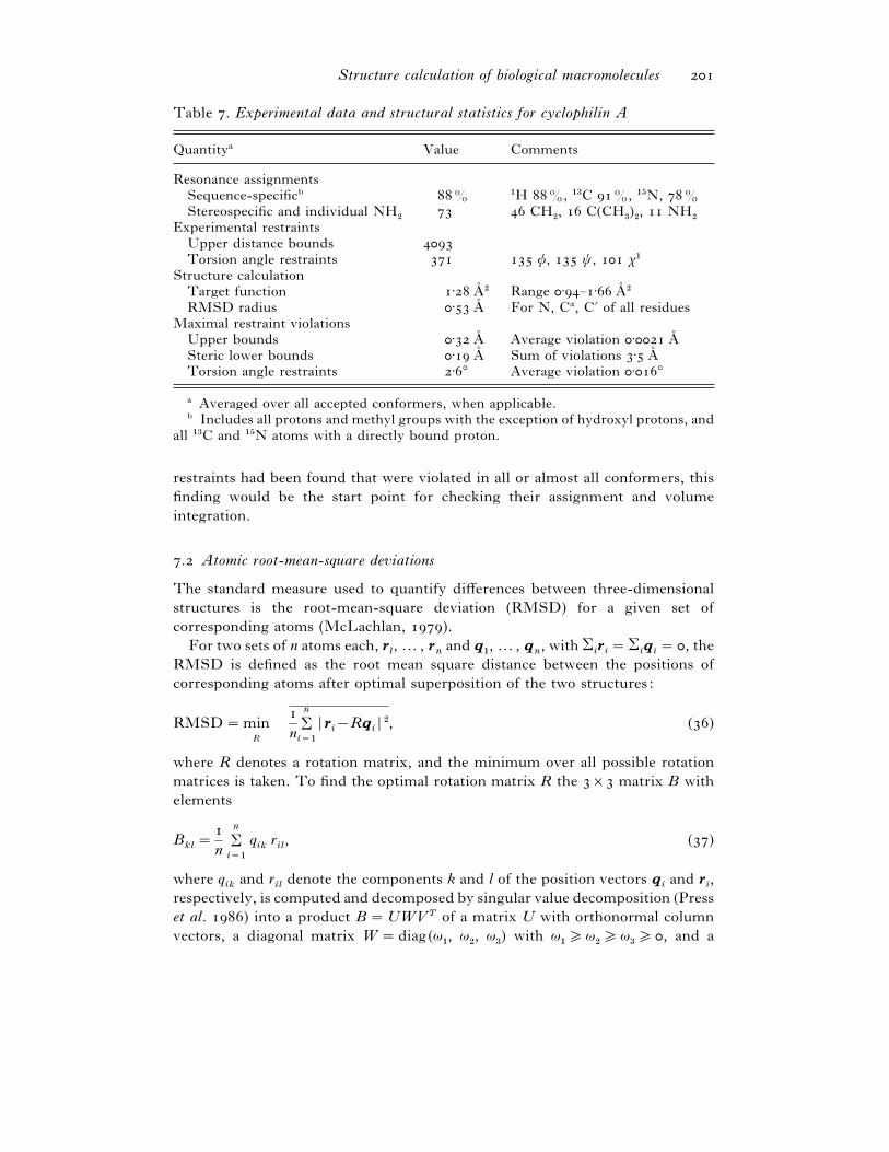
Structure calculation of biological macromolecules
Table . Experimental data and structural statistics for cyclophilin A
Quantitya Value Comments
Resonance assignments
Sequence-specificb % "H %, "$C %, "&N, %
Stereospecific and individual NH#
CH#, C(CH
$)#, NH
#Experimental restraints
Upper distance bounds Torsion angle restraints φ, ψ, χ"
Structure calculation
Target function ± AI # Range ±–± AI #RMSD radius ± AI For N, Cα, C« of all residues
Maximal restraint violations
Upper bounds ± AI Average violation ± AISteric lower bounds ± AI Sum of violations ± AITorsion angle restraints ±° Average violation ±°
a Averaged over all accepted conformers, when applicable.b Includes all protons and methyl groups with the exception of hydroxyl protons, and
all "$C and "&N atoms with a directly bound proton.
restraints had been found that were violated in all or almost all conformers, this
finding would be the start point for checking their assignment and volume
integration.
. Atomic root-mean-square deviations
The standard measure used to quantify differences between three-dimensional
structures is the root-mean-square deviation (RMSD) for a given set of
corresponding atoms (McLachlan, ).
For two sets of n atoms each, rl, … , r
nand q
", … , q
n, with 3
iri¯3
iq
i¯ , the
RMSD is defined as the root mean square distance between the positions of
corresponding atoms after optimal superposition of the two structures:
RMSD¯min
R
n3n
i="
r ri®Rq
ir #, ()
where R denotes a rotation matrix, and the minimum over all possible rotation
matrices is taken. To find the optimal rotation matrix R the ¬ matrix B with
elements
Bkl
¯
n3n
i="
qik
ril, ()
where qik
and ril
denote the components k and l of the position vectors qiand r
i,
respectively, is computed and decomposed by singular value decomposition (Press
et al. ) into a product B¯UWVT of a matrix U with orthonormal column
vectors, a diagonal matrix W¯diag(ω", ω
#, ω
$) with ω
"&ω
#&ω
$& , and a

Peter GuX ntert
Fig. . Overview output file of the program produced at the end of a structure
calculation using the experimental NMR data set for the protein cyclophilin A (Ottiger et al.
). The out of conformers with lowest final target function values were analysed.
The upper table shows, with one row for each conformer, the target function value,
followed by three restraint violation measures – the number of violations that exceed the
corresponding cutoff given at the top, the sum of violations, and the maximal violation – for
each of the four types of restraints : upper distance bounds, lower distance bounds (not used
in this calculation), steric lower distance bounds, and torsion angle restraints. Average
values, standard deviations, minima and maxima of these quantities are given below. The
second part of the file lists all restraint violations larger than the cutoffs and identifies the
conformer(s) in which they occur (‘ ’ and ‘n ’ signs in the columns on the right).

Structure calculation of biological macromolecules
Reference structure
BiasRadius
Individualconformers
Mean
Fig. . RMSD radius of a bundle of conformers, and RMSD bias of a bundle of
conformers with respect to a reference structure. The RMSD radius is the average of the
RMSD values between each individual conformer of the bundle and its mean coordinates.
The RMSD bias is the RMSD value between the mean coordinates of the bundle and a
reference structure. The mean coordinates of a bundle of n conformers are obtained by
superimposing for minimal RMSD the conformers , … , n onto the first conformer and
then averaging the Cartesian coordinates.
transposed orthogonal matrix V. The rotation matrix R that minimizes the
expression in equation () is then given by
R¯U diag(, , s)VT, ()
where s¯³ denotes the sign of the determinant of the matrix B and ensures that
R is a pure rotation with determinant (McLachlan, ). Without this
precaution incorrect (too small) RMSD values result if the mirror image of a
structure yields a better superposition than the structure itself.
The optimal superposition according to equation () is also used for the
simultaneous display of several conformers on a molecular graphics system
(Koradi et al. ). In practice, RMSD values are usually calculated for the
backbone atoms N, Cα and C«, or for all heavy (i.e. non-hydrogen) atoms of the
residues with well-defined conformation, excluding, for instance, chain termini
and loops that are unstructured in solution.
When RMSD values are used to measure the spread among the m conformers
in a structure bundle, the quantity with the most intuitive meaning is the ‘RMSD
radius’ (Fig. ), defined as the average of the m pairwise RMSD values between
the individual conformers and their mean structure. To compute the mean

Peter GuX ntert
180
90
0
–90
–180
–180 –90 0 90 180
w
φ
Fig. . Ramachandran plot for a bundle of conformers of the protein cyclophilin A. The
structures were calculated on the basis of the experimental NMR data set for cyclophilin A
(Ottiger et al. ) with the torsion angle dynamics algorithm of the program
(Gu$ ntert et al. ), which was also used to create the Ramachandran plot. Each circle
corresponds to the φ}ψ values of a non-glycine residue in one of the conformers. The
most favourable, additionally allowed, generously allowed, and disallowed regions according
to the program (Laskowski et al. ) are represented by dark, medium, light
and no shading, respectively.
structure, the conformers are superimposed for minimal RMSD onto the first
conformer, and the arithmetic mean of the corresponding Cartesian coordinates is
taken. As an alternative to the RMSD radius, the average of the m(m®)}
pairwise RMSD values among the individual conformers can be reported. This
quantity is in general about ± times larger than the corresponding RMSD radius.
The deviation of a structure bundle from a given ‘external ’ reference structure is
most easily described by the RMSD value between the mean coordinates of the
bundle and the reference structure, the ‘RMSD bias’ (Fig. ). RMSD radius and
RMSD bias have the intuitive geometric meaning of the radius of a tube
containing the structure bundle and the distance between the centre of the tube
and the reference structure, respectively (Fig. ).
It cannot be overemphasized that a small RMSD value is not by itself indicative
of a high-quality structure. It neither conveys any information about the
consistency with the experimental data nor does it necessarily correspond to the
conformation space that is really allowed by the conformational restraints because
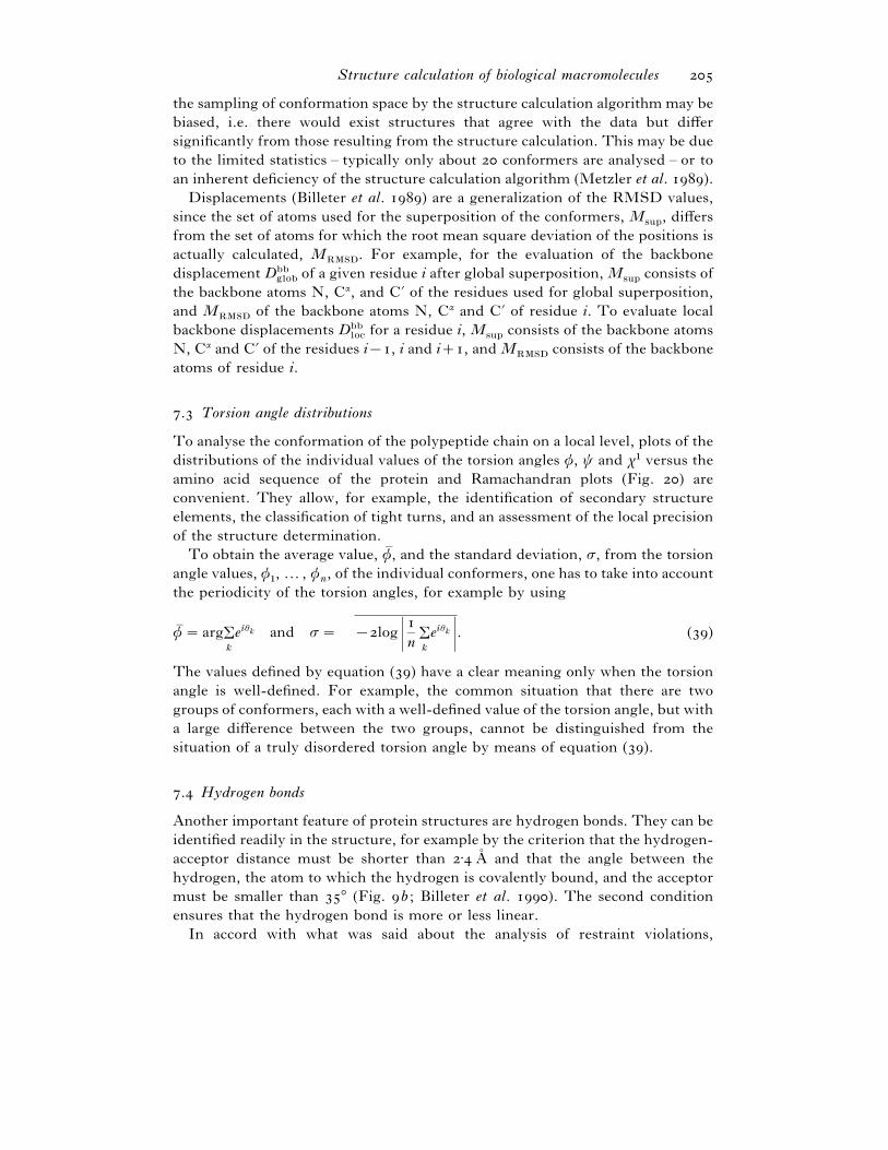
Structure calculation of biological macromolecules
the sampling of conformation space by the structure calculation algorithm may be
biased, i.e. there would exist structures that agree with the data but differ
significantly from those resulting from the structure calculation. This may be due
to the limited statistics – typically only about conformers are analysed – or to
an inherent deficiency of the structure calculation algorithm (Metzler et al. ).
Displacements (Billeter et al. ) are a generalization of the RMSD values,
since the set of atoms used for the superposition of the conformers, Msup
, differs
from the set of atoms for which the root mean square deviation of the positions is
actually calculated, MRMSD
. For example, for the evaluation of the backbone
displacement Dbbglob
of a given residue i after global superposition, Msup
consists of
the backbone atoms N, Cα, and C« of the residues used for global superposition,
and MRMSD
of the backbone atoms N, Cα and C« of residue i. To evaluate local
backbone displacements Dbbloc
for a residue i, Msup
consists of the backbone atoms
N, Cα and C« of the residues i®, i and i, and MRMSD
consists of the backbone
atoms of residue i.
. Torsion angle distributions
To analyse the conformation of the polypeptide chain on a local level, plots of the
distributions of the individual values of the torsion angles φ, ψ and χ" versus the
amino acid sequence of the protein and Ramachandran plots (Fig. ) are
convenient. They allow, for example, the identification of secondary structure
elements, the classification of tight turns, and an assessment of the local precision
of the structure determination.
To obtain the average value, φ- , and the standard deviation, σ, from the torsion
angle values, φ", … , φ
n, of the individual conformers, one has to take into account
the periodicity of the torsion angles, for example by using
φa ¯ arg3k
eiθk and σ¯ ®log ) n 3k
eiθk ). ()
The values defined by equation () have a clear meaning only when the torsion
angle is well-defined. For example, the common situation that there are two
groups of conformers, each with a well-defined value of the torsion angle, but with
a large difference between the two groups, cannot be distinguished from the
situation of a truly disordered torsion angle by means of equation ().
. Hydrogen bonds
Another important feature of protein structures are hydrogen bonds. They can be
identified readily in the structure, for example by the criterion that the hydrogen-
acceptor distance must be shorter than ± AI and that the angle between the
hydrogen, the atom to which the hydrogen is covalently bound, and the acceptor
must be smaller than ° (Fig. b ; Billeter et al. ). The second condition
ensures that the hydrogen bond is more or less linear.
In accord with what was said about the analysis of restraint violations,

Peter GuX ntert
significance should only be attributed to hydrogen bonds that occur consistently
in a sizeable number of conformers in a structure bundle. Since the geometric
force fields generally used for the structure calculation do not contain potentials
that favour the formation of hydrogen bonds, their abundance, counted according
to the criterion of Fig. , often increases considerably during a subsequent energy
refinement. On the other hand, the use of electrostatic potentials in vacuo tends to
yield spurious intra-protein hydrogen bonds (and salt bridges) on the surface of
the macromolecule (Guenot & Kollman, ; Luginbu$ hl et al. ), and should
be avoided.
. Molecular graphics
Molecular graphics programs are an indispensable tool to visualize and analyse
NMR structures. Thanks to real-time transformations, stereo displays and ray-
tracing techniques, three-dimensional impressions close to those of real, physically
built models can be produced routinely nowadays. Many molecular graphics
programs are available, for example the academic packages (Ferrin et al.
), (Nicholls et al. ), (Kraulis, ), (Sayle &
Milner-White, ), (Koradi et al. ), and the commercial products
(Molecular Simulations, Inc.) and (, Inc.).
The program (Koradi et al. ) is unique in the sense that it has been
designed especially for work with NMR structures that are represented by
bundles of conformers, which are often handled awkwardly by other programs. In
addition to high-quality molecular graphics, a wide array of structure analyses can
be performed with , including the calculation and display of mean
structures, restraint violations, hydrogen bonds, RMSDs, torsion angle
distributions, Ramachandran plots, and electrostatic surfaces. Fig. presents
four different representations of the solution structure of cyclophilin A that were
produced with the program : A schematic view (Fig. a) that emphasizes
the secondary structure elements: an eight-stranded antiparallel β-barrel that is
closed by two amphipathic α-helices, and a short "!
-helix of residues –
(Ottiger et al. ) ; a bundle of ten conformers (Fig. b) ; another schematic
view that illustrates the local precision of the structure by virtue of a tube with
variable diameter (Fig. c) ; and an all-heavy-atom representation of one
conformer overlaid with the dense network of distance restraints (Fig. d).
. Check programs
Programs have been developed to perform a ‘quality check’ of a structure
determined by X-ray crystallography or NMR spectroscopy. The best known
examples of such programs are (Laskowski et al. ), including its
NMR-specific extension - (Laskowski et al. ) and
(Vriend & Sander, ). These software packages try to assess the quality of a
structure primarily by checking whether a number of different parameters are in
agreement with their values in databases derived from high-resolution X-ray

Structure calculation of biological macromolecules
(a)
(c)
(b)
(d)
Fig. . Solution structure of the protein cyclophilin A, calculated using the torsion angle
dynamics algorithm of the program on the basis of the experimental NMR data set
collected by Ottiger et al. (). Displays produced with the program (Koradi et
al. ) : (a) Schematic representation highlighting α-helices and β-strands. (b)
Superposition of the ten conformers with lowest target function values. Only bonds between
the backbone atoms N, Cα and C« are drawn. (c) Another representation that affords an
impression of the variable precision of different parts of the polypeptide backbone. The
diameter of the hose-shaped object reflects the positional spread in the structure bundle
among the corresponding backbone atoms. (d ) One of the cyclophilin A conformers and the
network of distance restraints used in the structure calculation. The structure is represented
by dark cylinders for covalent bonds between heavy atoms; distance restraints are visualized
by thin lines. Intraresidual and sequential distance restraints have been omitted for clarity.
structures. Examples of such parameters include: correct values for covalent bond
lengths and bond angles (Engh & Huber, ), the percentage of residues with
φ}ψ-values in the most favoured regions of the Ramachandran plot, the clustering
of χ"-angles at the staggered rotamer positions, the overall quality of packing, the

Peter GuX ntert
absence of bad non-bonded contacts, the completeness of the hydrogen bonding
network (i.e. a minimal number of atoms with unsatisfied hydrogen bonding
capabilities in the core of the molecule), etc. Outliers of these quantities do not
necessarily point to errors in the structure – they occur, albeit rarely, also in X-ray
structures solved to very high resolution – but should be checked meticulously to
rule out a possible misinterpretation of the experimental data. In addition, check
programs like - (Laskowski et al. ) can read experimental
restraints in a variety of formats and provide measures for the agreement of the
experimental restraints with the structure calculated from them in a way that is
independent from the structure calculation program. Programs like also
look out for straightforward mistakes of the covalent structure, such as wrong
chiralities, which seem to occur disquietingly often in protein (Hooft et al. )
and nucleic acid structures (Schultze & Feigon, ). Of course, that a structure
fulfils the criteria of a check program does not guarantee it to be correct ; most
checks probe only local features of the conformation.
. A single, representative conformer
The usual representation of an NMR structure as a bundle of conformers, each of
which being an equally good fit to the data, provides a wealth of information about
the conformational uncertainty, which may be correlated to true flexibility of the
molecule. For example, alternative conformations of side-chains and complete
loops may be realized in different conformers, a feature that is difficult, if not
impossible, to represent in a single structure. Nevertheless, it is often desirable to
provide, in addition to the bundle of conformers, a single representative structure
that may be used in the same way as an X-ray structure, avoiding the bewildering
amount of detail in the bundle, for example in pictures or in comparisons of the
structures of different proteins.
Clearly, the Cartesian coordinates averaged over the conformers in the bundle
(after suitable superposition) are no good choice: they lie exactly in the centre of
the bundle, of course, but the averaging entails unacceptable distortions of the
covalent geometry. The average coordinates are thus only used as a reference for
the calculation of RMSD values, namely the RMSD radius of Fig. . Selecting
just one of the conformers in the bundle is another straightforward possibility. In
this case, the representative conformer has, by definition, the same quality as the
bundle. The selection can be random or based on different criteria, for instance,
smallest RMSD to the mean, smallest restraint violations, lowest conformational
energy, highest coincidence with the network of consistent hydrogen bonds in the
bundle, etc. Since all conformers in the bundle are essentially equivalent, the
choice should not be crucial. In general, there will exist structures (not members
of the bundle) that fulfil the restraints as well as those in the bundle but that lie
closer to its centre than any of its individual members, and hence the representative
conformer chosen from among them.
A procedure that can yield such a structure has been introduced by Clore et al.
(a) and is used routinely when structures are determined by simulated

Structure calculation of biological macromolecules
annealing in Cartesian space: From a bundle of conformers the mean structure is
computed and subsequently regularized by restrained energy minimization. This
results in general in a structure with good stereochemistry and in agreement with
the experimental data that is significantly closer to the mean coordinates of the
bundle than any of the individual conformers.
.
This chapter discusses a number of general aspects of NMR structure calculation
on the basis of the experimental NMR data set for cyclophilin A (Ottiger et al.
) for which structure calculations by torsion angle dynamics were performed
with the program (Gu$ ntert et al. ). An especially rich set of
experimental restraints is available for cyclophilin A (Table ) which affords a
particularly suitable platform for these investigations.
Table and Figs , and also show the results of a structure calculation
with the complete data set that will serve as a reference for various investigations
in this chapter. Fifty random start conformers were subjected to simulated
annealing according to the standard schedule of (see Section ..), and the
conformers with lowest final target function value were chosen to represent the
solution structure of the protein.
. Ensemble size
NMR structure calculations are always performed by computing, using the same
algorithm, many different conformers, each starting from another random initial
conformation. Provided that the input data set is self-consistent (as will be
assumed in the following), some of the conformers will be good solutions to the
problem, i.e. exhibit small restraint violations, whereas others might be trapped
in local minima. For this reason it is customary to compute an ensemble consisting
of more conformers than needed, and to select among them the ‘best ’ ones that
will represent the solution structure of the molecule and be analysed further.
Obviously, three choices have to be made in this process: How many conformers
should be computed in the first place? How many conformers should be used to
represent the solution structure? And how should these be selected from the
ensemble of all conformers? The answer to the second question is simple: , or
any other number that offers a reasonable compromise between sufficient statistics
and manageability in graphics and analysis programs. With regard to the third
question, it is clear that the selection of acceptable conformers should never rely
on a measure of conformational spread, for instance the RMSD value, but be
based on how well the experimental and steric restraints are fulfilled and, if the
structure calculation program worked in Cartesian space, how close the covalent
structure parameters are to their optimal values. Since the target function
measures exactly these parameters, the most obvious selection and almost
universally applied criterion is therefore to choose the N conformers with lowest
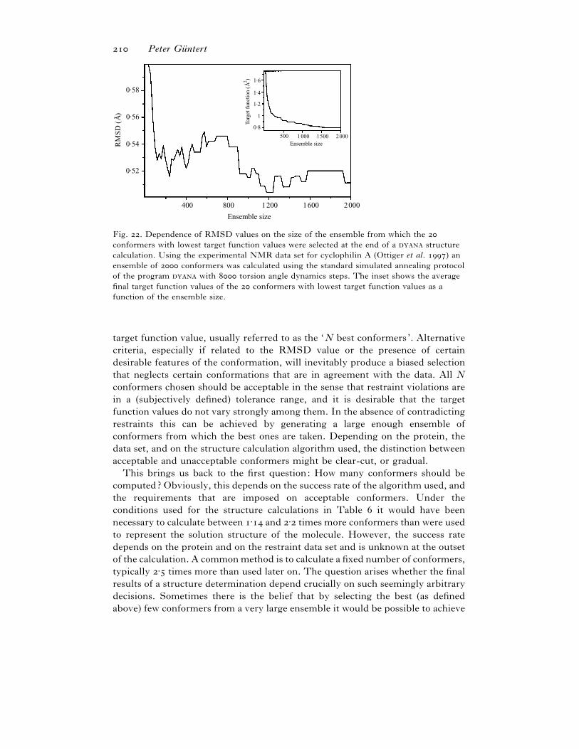
Peter GuX ntert
1·6
1·4
1·2
1
0·8
500 1000 1500 2000Ensemble size
Targ
et f
unct
ion
(Å2 )
0·58
0·56
0·54
0·52
400 800 1200 1600 2000
Ensemble size
RM
SD
(Å
)
Fig. . Dependence of RMSD values on the size of the ensemble from which the
conformers with lowest target function values were selected at the end of a structure
calculation. Using the experimental NMR data set for cyclophilin A (Ottiger et al. ) an
ensemble of conformers was calculated using the standard simulated annealing protocol
of the program with torsion angle dynamics steps. The inset shows the average
final target function values of the conformers with lowest target function values as a
function of the ensemble size.
target function value, usually referred to as the ‘N best conformers’. Alternative
criteria, especially if related to the RMSD value or the presence of certain
desirable features of the conformation, will inevitably produce a biased selection
that neglects certain conformations that are in agreement with the data. All N
conformers chosen should be acceptable in the sense that restraint violations are
in a (subjectively defined) tolerance range, and it is desirable that the target
function values do not vary strongly among them. In the absence of contradicting
restraints this can be achieved by generating a large enough ensemble of
conformers from which the best ones are taken. Depending on the protein, the
data set, and on the structure calculation algorithm used, the distinction between
acceptable and unacceptable conformers might be clear-cut, or gradual.
This brings us back to the first question: How many conformers should be
computed? Obviously, this depends on the success rate of the algorithm used, and
the requirements that are imposed on acceptable conformers. Under the
conditions used for the structure calculations in Table it would have been
necessary to calculate between ± and ± times more conformers than were used
to represent the solution structure of the molecule. However, the success rate
depends on the protein and on the restraint data set and is unknown at the outset
of the calculation. A common method is to calculate a fixed number of conformers,
typically ± times more than used later on. The question arises whether the final
results of a structure determination depend crucially on such seemingly arbitrary
decisions. Sometimes there is the belief that by selecting the best (as defined
above) few conformers from a very large ensemble it would be possible to achieve
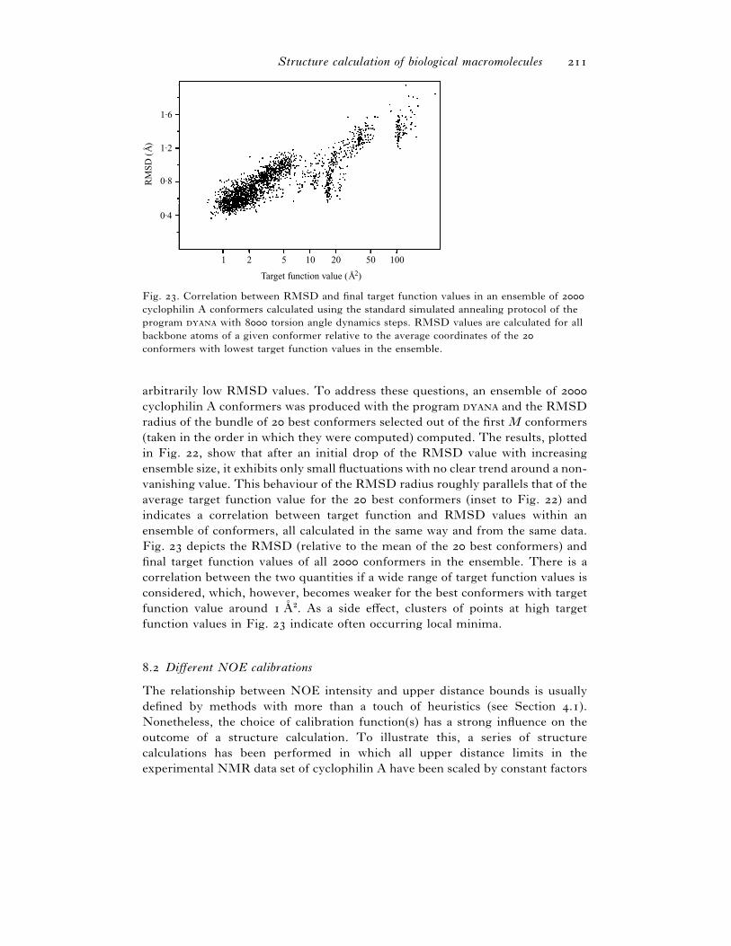
Structure calculation of biological macromolecules
1·6
1·2
0·8
0·4
1 2 5 10 20 50 100
Target function value (Å2)
RM
SD
(Å
)
Fig. . Correlation between RMSD and final target function values in an ensemble of
cyclophilin A conformers calculated using the standard simulated annealing protocol of the
program with torsion angle dynamics steps. RMSD values are calculated for all
backbone atoms of a given conformer relative to the average coordinates of the
conformers with lowest target function values in the ensemble.
arbitrarily low RMSD values. To address these questions, an ensemble of
cyclophilin A conformers was produced with the program and the RMSD
radius of the bundle of best conformers selected out of the first M conformers
(taken in the order in which they were computed) computed. The results, plotted
in Fig. , show that after an initial drop of the RMSD value with increasing
ensemble size, it exhibits only small fluctuations with no clear trend around a non-
vanishing value. This behaviour of the RMSD radius roughly parallels that of the
average target function value for the best conformers (inset to Fig. ) and
indicates a correlation between target function and RMSD values within an
ensemble of conformers, all calculated in the same way and from the same data.
Fig. depicts the RMSD (relative to the mean of the best conformers) and
final target function values of all conformers in the ensemble. There is a
correlation between the two quantities if a wide range of target function values is
considered, which, however, becomes weaker for the best conformers with target
function value around AI #. As a side effect, clusters of points at high target
function values in Fig. indicate often occurring local minima.
. Different NOE calibrations
The relationship between NOE intensity and upper distance bounds is usually
defined by methods with more than a touch of heuristics (see Section .).
Nonetheless, the choice of calibration function(s) has a strong influence on the
outcome of a structure calculation. To illustrate this, a series of structure
calculations has been performed in which all upper distance limits in the
experimental NMR data set of cyclophilin A have been scaled by constant factors

Peter GuX ntert
100
10
1
0·1
1·0
0·5
(a)
(b)
RM
SD
(Å
)Ta
rget
fun
ctio
n (Å
2 )
0·8 0·9 1 1·1 1·2 1·3
Distance limit scaling factor
RadiusBias
Fig. . Influence of scaling of the distance restraints on the outcome of structure
calculations with the experimental NMR data set for cyclophilin A (Ottiger et al. ). All
upper distance limits were scaled by the factor given on the horizontal axis. Ensembles of
conformers were calculated using the standard simulated annealing protocol of the program
with torsion angle dynamics steps, and the conformers with lowest target
function values were analysed. (a) Average final target function values. (b) RMSD radius
(solid), i.e. the average backbone RMSD values of the conformers relative to their mean
coordinates, and RMSD bias (dotted), i.e. the backbone RMSD value between the mean
coordinates of the bundles obtained with a given scaling factor and without scaling.
in the range of ± to ± in order to mimic equivalent changes of the calibration
constants k in equations () and (). A scaling factor of one corresponds to the
original experimental data set. The results, plotted in Fig. , show a strong
increase of the target function values with decreasing distance bounds (note the
logarithmic scale in Fig. a), and a less pronounced but clear increase of the
RMSD radius with increasing scaling factor (Fig. b). The RMSD bias of the
structure bundle obtained from scaled distance bounds relative to the mean
coordinates of the original bundle monotonically increases from a minimum at
scaling factor one in both directions (Fig. b). These findings indicate that target
function and RMSD values have no absolute meaning but depend strongly on the
NOE calibration used.
. Completeness of the data set
The collection of an extensive set of NOE distance restraints constitutes a major
part of the work involved in solving an NMR structure of a protein, and
progressively more effort is required (and increasingly difficult decisions have to
be taken) to assign additional NOEs, the more complete the data set becomes. In
the case of cyclophilin A, the NOESY spectra were analysed as exhaustively as
possible, resulting in a data set of about relevant distance restraints per residue
(Ottiger et al. ). Sometimes, however, such an effort might not be warranted,

Structure calculation of biological macromolecules
Table . DYANA structure calculations for the protein Cyclophilin A using the
complete experimental NMR data set and different subsets thereofa
Distance
Success
rate
Target
function
Backbone RMSD (AI )d
Data setb restraints (%)c (AI #) Radius Bias
All experimental
restraints
± ± ±
No stereospecific
assignments
e ± ± ±
No angle restraints ± ± ±% of all NOEsf
% ± ± ±% ± ± ±% ± ± ±% ± ± ±% ± ± ±
Only backbone
and Hβ NOEs
± ± ±
Only HN–HN NOEs ± ± ±
a For each data set conformers were calculated using the standard simulated
annealing protocol of the program with torsion angle dynamics steps and a
target function with linear asymptote for large violations. The conformers with the
lowest final target function values were analysed.b The different data sets were derived from the complete experimental NMR data set
for Cyclophilin A (Ottiger et al. ) that comprises meaningful upper distance
limits obtained from NOE measurements and restraints for the torsion angles φ, ψand χ". The same torsion angle restraints were included in all data sets except the one
without any torsion angle restraints.c Percentage of conformers with final target function values below f
min± AI #, where
fmin
is the lowest target function within the bundle (Gu$ ntert et al. ).d Radius: Average of the RMSD values between each individual conformer and
the mean coordinates of the bundle. Bias: RMSD value between the mean coordinates
of the bundle and the mean coordinates of the bundle obtained with the complete
experimental data set. The bias for the complete experimental data set was obtained by
performing two structure calculations with different initial structures.e This number exceeds that for the complete experimental data set because in the
absence of stereospecific assignments pairs of distance restraints to a diastereotopic pair
might be replaced by three restraints, two identical ones to the diastereotopic atoms and
one to the centrally located pseudoatom (see Section . ; Gu$ ntert et al. a).f Each individual distance restraint is retained with the given probability. Results are
averages over five different random selections.
and one might ask what quality of structure could be attained on the basis of a less
complete but more readily collected data set. To address this question, a number
of structure calculations were performed with subsets of the complete
experimental data set for cyclophilin A (Table ). The subsets were created
alternatively by retaining randomly only a certain percentage of all distance

Peter GuX ntert
restraints, by neglecting stereospecific assignments or torsion angle restraints, or
by restricting the data set to only backbone and Hβ NOEs or to only HN–HN
NOEs. As expected, the precision of the structure decreases with decreasing
information content of the data set (Table ). In parallel it becomes more difficult
for the structure calculation algorithm to find good solutions, i.e. the success rates
sink. However, the absence of stereospecific assignments, torsion angle restraints,
or up to % of the NOE distance restraints has only a moderate effect and does
not preclude the determination of a well-defined structure. Low resolution
structures can still be calculated from as little as % of the distance restraints,
or without any experimental restraints for the side-chain conformation beyond Cβ.
Not astonishingly, however, the success rate of the structure calculation was only
% in the absence of side-chain restraints, an unusually low value for the torsion
angle dynamics algorithm that presumably resulted from the difficulty to pack the
side-chains in the protein core. With only % of the NOEs it is no longer possible
to unambiguously determine the three-dimensional structure, and even less so if
only restraints among backbone amide protons are considered (Table ). The
latter result is in line with the findings of Venters et al. () and Smith et al.
() who have investigated the possibility of global fold determination using
deuterated protein samples and found that it would be necessary to measure
HN–HN distances up to AI to enable an unambiguous global fold determination.
. Wrong restraints and their elimination
In the course of a protein structure determination by NMR it is always possible
that NOEs with incorrect assignments enter the data set. The normal way to
detect and correct such mistakes is a careful analysis of restraint violations in the
structure calculated from the experimental data. Consistent violations, i.e. those
that occur in all or in a large majority of the conformers, are most likely not due
to imperfections of the structure calculation program but the result of restraints
that contradict each other. An ideal structure calculation method from the point
of view of error detection would pinpoint all mistakes by reporting consistent
violations for all wrong restraints, but not for any other (correct) restraints. In
practice, this is not the case because the structure calculation programs minimize
a target function that is a sum of contributions from all restraints, and to which
the largest violations contribute most. Hence, there is a tendency to ‘smear out’
the problem caused by a wrong restraint over other restraints in the vicinity to the
effect that either additional, correct restraints become consistently violated, or that
the problem is no longer recognized because it was distributed over many, only
slightly violated restraints. The latter problem is normally less severe in torsion
angle space than in Cartesian space, where slight, diffuse distortions of the
covalent geometry offer additional possibilities to disperse violations.
The ability of the torsion angle dynamics algorithm of to detect and
automatically eliminate erroneous restraints is illustrated in Table using data
sets from Table to which % of distance restraints with arbitrary, wrong

Structure calculation of biological macromolecules
Table . Structure calculations for Cyclophilin A with data sets to which first �%
distance restraints with wrong assignments were added and from which subsequently
consistently violated distance restraints were eliminateda
Restraints eliminated (%)b Target
function
Backbone RMSD (AI )c
Data set Wrong Correct (AI #) Radius Bias
All experimental
restraints
± ± ± ±
No stereospecific
assignments
± ± ± ±
No angle restraints ± ± ± ±% of all NOEs
% ± ± ± ±% ± ± ± ±% ± ± ± ±% ± ± ± ±% ± ± ± ±
Only backbone
and Hβ NOEs
± ± ± ±
a Wrong distance restraints were generated by selecting distance restraints arbitrarily
from the complete experimental data set and replacing one of the two atoms by an
arbitrarily chosen different atom for which the "H chemical shift was available. The
second atom and the upper distance limit of the restraint remained unchanged. With
these wrong restraints added to each data set bundles of conformers were calculated
using the same protocol as in Table . Consistently violated distance restraints, i.e. those
that are violated by more than ± AI in or more of the conformers, were then
eliminated in two steps. In the first round, the % consistently violated distance
restraints with the largest average violations were deleted, and the structure calculation
was repeated. In the second round, all remaining consistently violated distance restraints
were eliminated, and the structure calculation was repeated again. The resulting conformers for each data set were analysed.
b Number of wrong distance restraints eliminated, given as a percentage of the total
number of wrong distance restraints that were added to the data set, and number of
correct distance restraints eliminated, given as a percentage of the total number of
distance restraints in the original data set without wrong restraints.c RMSD radius and bias are defined as in Table .
assignments have been added. Incorrect restraints were detected and eliminated in
three rounds of structure calculations where consistent violations found at the end
of the first and second round were removed from the data set that became the
input for the following structure calculation. The results (Table ) show that with
good data sets around % of the erroneous restraints could be detected by this
straightforward automatic method, and that significantly less than % of the
correct restraints were falsely eliminated. The resulting structures are of similar
quality as those obtained from correct restraints only, and there is close agreement
between them. In the case of sparse data sets, however, the discriminatory power

Peter GuX ntert
of the procedure deteriorates to the point that only % of the wrong restraints
can be found and removed from the data sets comprising one tenth of all NOEs.
The many wrong NOEs remaining in the data set lead to significantly higher
target function values than the calculations with exclusively correct restraints.
.
The assignment of cross peaks in NOESY spectra for the collection of NOE upper
distance limits on "H–"H distances is an essential part of the determination of
three-dimensional protein structures in solution by NMR. Obtaining NOESY
cross peak assignments is usually a laborious endeavour, particularly in spectral
regions where chemical shift degeneracies result in excessive cross peak overlap.
Were it not for these inevitable chemical shift degeneracies and the usually
somewhat imprecise cross peak positional information, all assignments could of
course be made in a straightforward manner based on the knowledge of the
chemical shifts resulting from the sequence-specific resonance assignments. In
practice, however, only a fraction of the NOESY cross peaks can be assigned in
this direct way and subsequently used to generate a preliminary, ‘ low resolution’
structure of the protein under investigation. Subsequently, these preliminary
conformers may be used to reduce the number of previously ambiguous
assignments by eliminating pairs of protons which have the chemical shift
coordinates of the cross peak considered but, on the basis of the preliminary
solution structure, are further apart than a predetermined maximum distance
cutoff for the observation of NOEs. The collection of an extensive set of distance
restraints and the calculation of a high-quality structure are thus not separate,
subsequent steps of an NMR structure determination but intertwined in an
iterative process (Fig. a), regardless of whether exclusively manual,
semiautomatic (Gu$ ntert et al. ; Meadows et al. ) or automatic methods
(Mumenthaler & Braun, ; Mumenthaler et al. ; Nilges, ; Nilges et
al. ) are employed.
. Chemical shift tolerance range
The two fundamental requirements for a valid NOE assignment are agreement
between chemical shifts and the peak position, and spatial proximity in a
(preliminary) structure (Fig. b). Typically only a minority of the NOESY cross
peaks can be assigned unambiguously based on chemical shift agreement alone
because of inevitable small uncertainties in the determination of chemical shifts
and peak positions. Such inaccuracies require the introduction of a non-vanishing
chemical shift tolerance ∆tol
for the agreement between a "H chemical shift and a
peak position. The size of ∆tol
, that is the accuracy of chemical shift and peak
position determination, has a very pronounced influence on the number of
possible assignments for an NOE cross peak. This can be rationalized as follows
(Mumenthaler et al. ).

Structure calculation of biological macromolecules
(a) (b) Conditions for valid NOESY assignmentsAmino acid sequenceSequence-specificassignmentPositions and volumesof NOESY cross peaks
Find NOEassignments
Structurecalculation
Evaluate NOEassignments
NOE assignments
3D structure
Atom A
Atom B
dAB < dmax
xA
xB
Dtol
Peak at(x1, x2)
|x1 – xA| < Dtol,|x2 – xB| < Dtol
Fig. . (a) Flowchart of the iterative process of NOESY cross peak assignment and
structure calculation. (b) The two conditions that must be fulfilled by valid NOESY cross
peak assignments: Agreement between chemical shifts and the peak position, and spatial
proximity in a (preliminary) structure.
In a two-dimensional NOESY spectrum with N cross peaks for a protein
containing n hydrogen atoms with chemical shifts distributed evenly over a region
of width ∆ω, the probability of finding a "H shift in an interval [ω®∆tol
, ω∆tol
]
about any selected position ω is
p¯∆
tol
∆ω. ()
In the absence of structural information, the number of peaks that can be assigned
unambiguously based on the agreement of chemical shifts within the tolerance is
expected to be
N(")¯N(®p)#n−#ENe−#np. ()
Equation () predicts that the percentage of peaks that can be assigned
unambiguously without knowledge of a preliminary structure decreases
exponentially with increasing size of the protein and increasing tolerance range.
The number of peaks with exactly two assignment possibilities is expected to be
N(#)¯Np(n®) (®p)#n−$E npN("). ()
N(#) vanishes for very small ∆tol
values, but increases linearly as a function of
N(") with a coefficient that is proportional to the protein size and the ∆tol
value. At
∆tol
¯ ± ppm, N(#) is usually – times larger than N("). Fig. shows that the
simple model of equations ()–() provides a remarkably good description of the
situation in a real protein.
For peak lists obtained from "$C- or "&N-resolved D ["H,"H]-NOESY spectra,

Peter GuX ntert
1600
1200
800
400
0
N (1) N (2)
1600
1200
800
400
00 0·01 0·02 0 0·01 0·02
(a) Peaks with one assignment possibility
(b) Peaks with two assignment possibility
Chemical shift tolerance Dtol (ppm)
Fig. . Numbers of cross peaks with exactly one (N("), shown in (a)) or exactly two (N(#),
shown in (b)) possible assignments on the basis of agreement between "H chemical shifts
and the peak positions within a tolerance ∆tol
in a two-dimensional NOESY spectrum of the
protein WmKT (Antuch et al. ). No structural information has been used to resolve
ambiguities. The NOESY peak list was simulated on the basis of the experimental chemical
shift list by postulating a cross peak between any pair of protons separated by less than AIin the best NMR conformer (Antuch et al. ). In both (a) and (b) the curved lines
represent the corresponding values predicted by equations () and () for N¯ peaks,
n¯ protons, and a spectral width of ∆ω¯ ppm.
the ambiguity in the proton dimension correlated to the hetero-spin is normally
resolved. Equation () then adopts the form
N(")ENe−np. ()
The expected percentage of unambiguously assigned peaks is thus the same as in
a two-dimensional NOESY spectrum for a protein of half the size, or for half the
chemical shift tolerance.
In order to assign the majority of the NOESY cross peaks, the ambiguity of
assignments based exclusively on chemical shifts must be resolved by reference to
a preliminary structure. The ambiguity is resolved completely if all but one of the
potential assignments correspond to pairs of hydrogen atoms separated by more
than a maximal distance dmax
for which a NOE may be observed. Assuming that
the hydrogen atoms are evenly distributed within a sphere of radius R that
represents the protein, the probability q to find two randomly selected hydrogen
atoms closer to each other than dmax
is given approximately by the ratio between
the volumes of two spheres with radii dmax
and R, respectively:
q¯ 0dmax
R 1$. ()
For a nearly spherical protein with radius R¯ AI and dmax
¯ AI this
probability becomes approximately %, indicating that only % of the peaks
with two assignment possibilities can be assigned uniquely by reference to the
protein structure. The total number of uniquely assigned peaks, Nunique
, can be
increased optimally to
Nunique
¯N(")(®q)N(#)(®q)#N($)… ()

Structure calculation of biological macromolecules
Even by reference to a perfectly refined structure it is therefore impossible, on
fundamental grounds, to resolve all assignment ambiguities because q will never
vanish and hence Nunique
!N.
. Semiautomatic methods
Semiautomatic NOE assignment methods provide for each NOESY cross peak a
list of the assignment possibilities according to the criteria of Fig. b. These are
analysed by the spectroscopist who may be able to further reduce their number by
visual inspection of the corresponding cross peaks and line shapes in the NOESY
spectrum. Peaks that can be assigned unambiguously by this method are added to
the input data set for the next round of structure calculation. The program
(Gu$ ntert et al. ) that is normally used in conjunction with the interactive
spectrum analysis program (Bartels et al. ) uses this principle for
automated removal of ambiguities arising from chemical shift degeneracies and
thus supports the collection of an extensive set of NOE distance restraints in
several rounds of NOESY cross peak assignments and structure calculations.
. Ambiguous distance restraints
An elegant approach to the NOE assignment problem was introduced by Nilges
(, ) who accounted for the ambiguity in the purely chemical-shift-based
NOE assignments by ‘ambiguous distance restraints ’, i.e. by interpreting the peak
volumes as r−'-weighted sums of contributions from all possible peak assignments
in the NOE target function. Ambiguous distance restraints are thus a
generalization of the r−'-summation method of equation () that can be applied
to restraints with diastereotopic protons in the absence of stereospecific
assignments. An optimization procedure based on simulated annealing by
molecular dynamics was described that is capable of using highly ambiguous input
data for ab initio structure calculations, where it is possible to specify the restraint
list directly in terms of the proton chemical shift assignment and the NOESY
cross peak positions (Nilges, ). This procedure was applied in structure
calculations of the basic pancreatic trypsin inhibitor (BPTI) from simulated
NOESY spectra (Nilges, ), and has been used also for the calculation of
symmetric oligomeric structures from NMR data, where all peaks are a
superposition of at least two NOE signals (Nilges, ; Donoghue et al. ).
In contrast to the normal manual approach, in which unambiguous assignments
are sought and peaks that cannot be assigned unambiguously are not used in the
structure calculation, the notion of ambiguous distance restraints allows one to
exploit the information carried by all NOESY cross peaks, regardless of whether
a peak has a unique assignment possibility or not. There are always some NOESY
cross peaks that reflect contributions from more than one spatially proximate
proton pair; these can be treated more realistically by ambiguous distance
restraints than by uniquely assigned NOEs.
Recently, Nilges et al. () have proposed a novel structure calculation
Peter GuX ntert
(a) Cycle 12 (b) Cycle 16 (c) Final structure
Fig. . Structures of the SH domain of human p Lck tyrosine kinase (Hiroaki et al.
; M. Salzmann, unpublished) at various stages of the automated combined NOESY
assignment and structure calculation method of Mumenthaler et al. (). The calculation
is based on the experimental NMR data set. Shown are backbone superpositions of ten
conformers at the end of the intermediate cycles (a) and (b), as well as the final
structure (c).
method that combines ambiguous distance restraints with an iterative assignment
strategy (see next section), whereby unambiguous assignments can be derived for
many NOE cross peaks that were entered into the calculation initially as
ambiguous restraints.
. Iterative combination of NOE assignment and structure calculation
An alternative approach for automatic NOESY assignment was proposed
(Mumenthaler & Braun, ; Mumenthaler et al. ) that uses as input only
the chemical shift lists obtained from the sequence-specific resonance assignment
and a list of NOESY cross peak positions. Ambiguous peak assignments are
treated as separate distance restraints in the structure calculations, and erroneous
assignments are eliminated in iterative cycles. An error-tolerant target function
reduces the impact of erroneous restraints on the calculated structures. In contrast
to the approach of Nilges (), noise and artifact peaks can be removed
automatically during the procedure, and peaks are ultimately assigned to single
proton pairs. This allows a critical comparison of the NOE assignments obtained
automatically with those from manual procedures not only on the level of the final
structures but also on the level of individual NOE assignments.
The method of Mumenthaler et al. () performs normally cycles of
automatic assignment and structure calculation (Fig. ), each with the three main
steps given in Fig. a. For the NOE assignment step in Fig. a, a list of the
assignment possibilities based on a given chemical shift tolerance ∆tol
is prepared.
In the first cycle, when no structural information is available, this list is used
directly. Otherwise, i.e. from the second cycle onwards, the preliminary structure
available from the preceding cycle is used to eliminate assignment possibilities
that correspond to proton pairs further apart than a limiting distance dmax
which
Structure calculation of biological macromolecules
is decreased linearly from ± AI in the first to ± AI in the last cycle. Using the
automatic calibration method described in Section ., new distance restraints are
then added as ‘test assignments’ to the input for the structure calculation for all
so far unassigned NOESY cross peak with less than M assignment possibilities,
where M¯ for the first cycles, M¯ for cycles –, and M¯ for cycles
–. It is necessary to use M" because otherwise the low number of
unambiguous assignments at the outset would preclude convergence to a well-
defined structure. In the structure calculation step of Fig. a an ensemble of
conformers is calculated using the standard protocol of the program
(Gu$ ntert et al. ). Because for a given peak up to M different restraints, of
which normally only one will turn out to be correct, are included in the input data
for the structure calculation it is important to use a functional form of the target
function that will not be dominated too much by strongly violated restraints
(Mumenthaler & Braun, ). In the NOE evaluation step of Fig. a the ten
conformers with lowest target function values are analysed. Each peak for which
test assignments have been added to the input is transferred either to the list of
unambiguous assignments, or returned to the list of unassigned peaks, which will
be analysed again in the next cycle. Peaks that have been classified as unambiguous
in previous cycles can be reclassified if the corresponding distance restraint is
violated in most conformers.
Applications of this procedure to the experimental data sets for six proteins are
summarized in Table (Mumenthaler et al. ). For all six proteins nearly
complete sequence-specific resonance assignments were available, and their
solution structure had been calculated on the basis of manually assigned NOE
cross peaks. The start point for the automatic procedure were the original peak
lists from which all assignments were deleted. Tolerance ranges ∆tol
of ±, ±
and ± ppm were used for protons in two-dimensional NOESY spectra, three-
dimensional NOESY spectra of Pa, and three-dimensional NOESY spectra of
DnaJ, respectively. The NOE assignments and the structures obtained from the
automatic procedure closely resemble those obtained from manually made
assignments. On average, the extent of assignments is somewhat lower from the
automatic method, and different assignments by the two approaches were
obtained for less than % of the peaks. The target functions and RMSD radii of
the final structures were comparable, and the automatically determined structures
show little bias from the original structures (Table ).
Further calculations conducted by Mumenthaler et al. () showed that the
automatic assignment method was remarkably robust with respect to imperfect
NOE peak lists and could produce acceptable structures from incomplete NOE
input. In contrast, the method was quite susceptible to incomplete "H chemical
shift lists. In spite of the progress made with the automatic method,
spectroscopists working interactively with NOESY spectra still have several
advantages because they can exclude assignment possibilities by line shape
considerations and often intuitively use smaller tolerance ranges between peak
positions and chemical shifts. This contributes in general to a more complete
NOESY assignment by the interactive method than by the automated approach.

Peter GuX ntert
Table
.S
truct
ure
calc
ula
tions
using
manually
and
auto
matica
lly
ass
igned
NO
ES
Ypea
klist
sa
Quantity
Er-
H
irudin
Wm
KT
DnaJ
Pa
Siz
eand
experi
menta
lin
put
data
Resi
dues
NO
ESY
spectr
ab
HD
HD
HH
NC
HD
NC
NO
ESY
cro
sspeaksc
Perc
enta
ge
of
peaks
(%)d
Manually
ass
igned
Auto
matically
ass
igned
Identically
ass
igned
Diff
ere
ntly
ass
igned
±
±
±
±
±
±
Inconsi
stente
±
±
±
±
±
±
Str
uctu
res
obta
ined
from
manualass
ignm
ent
Targ
et
function
valu
e(A
I#)
±
–±
±
–±
±
–±
±
–±
±
–±
±
–±
RM
SD
radiu
s(AI
)f±
±
±
±
±
±
Str
uctu
res
obta
ined
from
auto
matic
ass
ignm
ent
Targ
et
function
valu
e(A
I#)
±
–±
±
–±
±
–±
±
–±
±
–±
±
–±
RM
SD
radiu
s(A
I )f
±
±
±
±
±
±
RM
SD
bia
s(A
I )g
±
±
±
±
±
±
aE
xperi
menta
lN
OE
SY
peak
list
sets
for
the
follow
ing
pro
tein
sw
ere
use
d:
Er-
:
phero
mone
Er-
fr
om
Euplo
tes
raik
ovi
(Ott
iger
etal.
);
Hir
udin
:
hir
udin
(–)
(Szypers
ki
etal.
);
:
-r
epre
ssor(
–)
with
muta
tion
RM
(Perv
ush
inet
al.
);
Wm
KT
:yeast
kille
rto
xin
Wm
KT
(Antu
ch
etal.
);D
naJ:m
ole
cula
rchapero
ne
DnaJ(
–)(P
ellecchia
etal.
);Pa:path
ogenesi
s-re
late
dpro
tein
Pa
from
tom
ato
(Fern
a !ndez
etal.
).
Data
for
stru
ctu
res
obta
ined
by
manualass
ignm
entare
from
the
ori
gin
alpublications.
Auto
matic
ass
ignm
entw
as
perf
orm
ed
in
itera
tive
cycle
sofN
OE
ass
ignm
ent
and
stru
ctu
recalc
ula
tion
(Mum
enth
ale
ret
al.
).
Str
uctu
recalc
ula
tions
were
perf
orm
ed
with
the
pro
gra
ms
or
usi
ng
the
vari
able
targ
etfu
nction
meth
od
with
redundant
tors
ion
angle
rest
rain
ts(G
u $nte
rt&
Wu $th
rich,
).
bH
:tw
o-d
imensi
onal["
H,"H
]-N
OE
SY
inH
#
O;D
:tw
o-d
imensi
onal["
H,"H
]-N
OE
SY
inD
#
O;N
:"&N
-reso
lved
thre
e-d
imensi
onal["
H,"H
]-N
OE
SY
;C
:"$C
-reso
lved
thre
e-d
imensi
onal
["H
,"H
]-N
OE
SY
.c
Tota
lnum
ber
of
cro
sspeaks
inall
NO
ESY
spectr
ause
d.
dA
llperc
enta
ges
are
rela
tive
toth
eto
tal
num
ber
of
NO
ESY
cro
sspeaks.
ePerc
enta
ge
of
peaks
that
are
inconsi
stent
with
the
finalst
ructu
reobta
ined
by
auto
matic
ass
ignm
ent.
For
these
peaks
every
poss
ible
ass
ignm
ent
within
the
chem
ical
shift
tole
rance
range
isvio
late
dby
more
than
AI
inall
confo
rmers
.f
RM
SD
radii
of
the
confo
rmers
use
dto
repre
sent
the
solu
tion
stru
ctu
re,
com
pute
dfo
rth
ebackbone
ato
ms
N,
Cα,
C«
of
the
follow
ing
resi
dues:
Er-
,
–;
Hir
udin
,–
and
–;
,
–;
Wm
KT
,–
and
–;
DnaJ,
–;
Pa,
–.
gR
MSD
bia
sto
the
mean
coord
inate
sof
the
stru
ctu
rebundle
obta
ined
from
manual
ass
ignm
ent.
Structure calculation of biological macromolecules
.
There exist many possibilities for the refinement of NMR structures of proteins.
The following brief overview can only mention a few often used refinement
methods.
. Restrained energy minimization
The structure calculation algorithms for NMR structures usually use a simplified
force field that contains only the most dominant parts of the conformational
energy. Therefore, the resulting structures may be unfavourable with respect to a
full, ‘physical ’ energy function (Momany et al. ; Brooks et al. ; Cornell
et al. ; van Gunsteren et al. ) that includes, in addition to the terms used
by the structure calculation algorithms of Section , also a Lennard-Jones
potential and electrostatic interactions for non-bonded atom pairs, torsion angle
potentials, and possibly other terms. The conformational energy of a conformation
obtained from a structure calculation program can be reduced significantly by
restrained energy minimization, i.e. by locating a local minimum of the
conformational energy function in the near vicinity of the input structure.
Restrained energy minimization of a correct structure results in only small
changes of the conformation (Billeter et al. ). Because no large-scale
conformational changes are necessary, the restraining potentials for distance and
angle restraints may be chosen steeper than in the preceding structure calculation,
thereby reducing the maximal restraint violations. Potentials proportional to the
sixth (instead of second) power of the distance restraint violation have been used
frequently (Billeter et al. ). Generally the extent and regularity of hydrogen
bonds shows a marked improvement upon energy minimization because the
geometric force fields used for the structure calculation normally do not contain
a driving force for hydrogen bond formation (unless explicit hydrogen bond
restraints were used, of course). Since the solvent surrounding the macromolecule
is very important for a realistic representation of electrostatic interactions,
restrained energy minimizations should be performed in a box or shell of explicit
water molecules. Energy minimization in vacuo exaggerates electrostatic
interactions and can lead to artifacts such as charged and polar side-chains on the
protein surface that bend back to the protein, forming spurious salt-bridges and
hydrogen bonds (Luginbu$ hl et al. ).
. Molecular dynamics simulation
An unrestrained or restrained molecular dynamics simulation under physiological
conditions using the full physical force field and explicit water to represent the
solvent can often give new insights into a protein structure, in particular for the
generally disordered protein surface (McCammon & Harvey, ; Brooks et al.
; van Gunsteren & Berendsen, ). Such molecular dynamics simulations
try to represent the solvated molecular system as faithfully as possible and are
Peter GuX ntert
fundamentally different from simulated annealing, where artificial conditions such
as high temperature are chosen in order to enhance the sampling of conformation
space. A limiting factor in molecular dynamics simulations are the relatively short
simulation times of up to a few nanoseconds that are feasible with present
computers, because many motions in proteins occur on longer time scales.
. Time- or ensemble averaged restraints
The commonly used structure calculation algorithms try to find rigid
conformations that fulfill all distance and torsion angle restraints simultaneously,
and the effects of internal mobility of the polypeptide chain are taken into account
implicitly by interpreting the NOE data as conservative upper distance bounds
instead of exact distance restraints (Wu$ thrich, ). In reality, the NOEs and
scalar coupling constants measured by NMR constitute an average over time and
space. Methods have been devised to include distance and torsion angle restraints
as time-averaged rather than instantaneous restraints into a molecular dynamics
simulation (Kessler et al. ; Pearlman & Kollman, ; Torda et al. ,
, ; van Gunsteren et al. ). In another approach, a molecular
dynamics simulation is performed simultaneously for an ensemble of conformers,
such that the restraints are not required to be fulfilled by each individual
conformer but only by the ensemble as a whole (Scheek et al. ; Bonvin &
Bru$ nger, , ).
. Relaxation matrix refinement
Both spin diffusion and internal mobility influence the NOE intensities from
which distance restraints are derived for the structure calculation. Complete
relaxation matrix refinement (Keepers & James, ; Boelens et al. ; Yip &
Case, ) can, in principle, take these factors into account and thus may make
it possible to make more quantitative use of the NOE data as with the initial rate
approximation (Kumar et al. ) and the semi-quantitative calibration of
distance restraints (Wu$ thrich, ). However, there can be a danger of
overinterpreting the data because many of the parameters entering the relaxation
matrix cannot be measured experimentally. In particular, assumptions are needed
about internal and overall motions of the protein (Macura & Ernst, ). Two
different methods of complete relaxation matrix refinement are in use: Either the
relaxation matrix treatment is used to derive a more precise set of distance
restraints, which is then used in a conventional structure calculation (Keepers &
James, ; Boelens et al. ), or the three-dimensional structure may be
refined directly against the observed NOE intensities (Borgias & James, ; Yip
& Case, ; Mertz et al. ). The second approach is conceptually more
attractive but also more time-consuming. In analogy to the practice in X-ray
crystallography, it is possible to define R-factors that measure the agreement
between the NOESY spectrum and the three-dimensional structure (Gonzales et
al. ; Thomas et al. ; Withka et al. ).

Structure calculation of biological macromolecules
.
I thank Prof. Kurt Wu$ thrich for generous support, Mr Michael Salzmann for
providing Fig. , and Prof. Martin Billeter for helpful discussions. The use of the
computing facilities of the Competence Centre for Computational Chemistry of
ETH Zu$ rich is gratefully acknowledged.
.
A, R. & T, M. (). Biased probability Monte Carlo conformational
searches and electrostatic calculations for peptides and proteins. J. Mol. Biol. ,
–.
A, H., B, W., N, T. & G, N. (). Rapid calculation of first and second
derivatives of conformational energy with respect to dihedral angles in proteins.
General recurrent equations. Computers & Chemistry , –.
A, A. (). Principles of Nuclear Magnetism. Oxford: Clarendon Press.
A, B. J. & W, T. E. (). Studies of molecular dynamics. I. General
method. J. Chem. Phys. , –.
A, M. P. & T, D. J. (). Computer Simulation of Liquids. Oxford:
Clarendon Press.
A, R. B. & J, O. (). New strategies for the determination of
macromolecular structure in solution. J. Biochem. , –.
A, R. B. & J, O. (). Heuristic refinement method for determination
of solution structure of proteins from nuclear magnetic resonance data. Meth.
Enzymol. , –.
A, W., G$ , P. & W$ , K. (). Ancestral βγ-crystallin precursor
structure in a yeast killer toxin. Nature Struct. Biol. , –.
A, V. I. (). Mathematical Methods of Classical Mechanics. New York:
Springer.
A, A. S., K, V. I., M, V. N. & B, V. F. (). NMR
solution spatial structure of ‘short ’ scorpion insectotoxin I&A. FEBS Lett. , –.
B, D. S. & H, E. J. (). A recursive formulation for constrained mechanical
system dynamics: Part I. Open loop systems. Mech. Struct. Mech. , –.
B, L., B, I., B, K. L., C, M. A., G, H. B., L, C. &
T, P. (). The use of pseudocontact shifts to refine solution structures of
paramagnetic metalloproteins: MetAla cyano-cytochrome c as an example. J. Biol.
Inorg. Chem. , –.
B, C., X, T., B, M., G$ , P. & W$ , K. (). The
program for computer-supported NMR spectral analysis of biological
macromolecules. J. Biomol. NMR , –.
B, D. (). Some multistep methods for use in molecular dynamics calculations.
J. Comput. Phys. , –.
B, H. J. C., P, J. P. M., G, W. F., DN, A. & H,
J. R. (). Molecular dynamics with coupling to an external bath. J. Chem. Phys. ,
–.
B, K. D., G$ , P., O, L. P. M. & W$ , K. (). Determination
of a high-quality NMR solution structure of the bovine pancreatic trypsin inhibitor
(BPTI) and comparison with three crystal structures. J. Mol. Biol. , –.
Peter GuX ntert
B, F. C., K, T. F., W, G. J. B., M, E. F., J., B, M. D.,
R, J. R., K, O., S, T. & T, M. (). The Protein
Data Bank: a computer-based archival file for macromolecular structures. J. Mol.
Biol. , –.
B, C., R, C. B., L, B. A. & M, G. T. (). Multi-
dimensional NMR experiments and analysis techniques for determining homo- and
heteronuclear scalar coupling constants in proteins and nucleic acids. Adv. Biophys.
Chem. , –.
B, M., B, W. & W$ , K. (). Sequential resonance assignments in
protein "H nuclear magnetic resonance spectra. Computation of sterically allowed
proton-proton distances and statistical analysis of proton-proton distances in single
crystal protein conformations. J. Mol. Biol. , –.
B, M., H, M. & W$ , K. (). The ellipsoid algorithm as a method
for the determination of polypeptide conformations from experimental distance
constraints and energy minimization. J. Comp. Chem. , –.
B, M., K, A. D., B, W., H, R. & W$ , K. ().
Comparison of the high-resolution structures of the α-amylase inhibitor tendamistat
determined by nuclear magnetic resonance in solution and by X-ray diffraction in
single crystals. J. Mol. Biol. , –.
B, M., S, T., B, W. & W$ , K. (). Restrained energy
refinement with two different algorithms and force fields of the structure of the α-
amylase inhibitor tendamistat determined by NMR in solution. Biopolymers ,
–.
B, L. M. (). Theory and Applications of Distance Geometry. Cambridge,
UK: Cambridge University Press.
B, R., K, T. M. G., M, G. A., B, J. H. & K,
R. (). Iterative procedure for structure determination from proton–proton NOEs
using a full relaxation matrix approach. Application to a DNA octamer. J. Magn.
Reson. , –.
B A. M. & B$ , A. T. (). Conformational variability of solution nuclear
magnetic resonance structures. J. Mol. Biol. , –.
B A. M. & B$ , A. T. (). Do NOE distances contain enough information
to assess the relative populations of multi-conformer structures? J. Biomol. NMR ,
–.
B, B. A. & J, T. L. (). , a method for constrained refinements
of macromolecular structure based on two-dimensional nuclear Overhauser spectra. J.
Magn. Reson. , –.
B, C. & T, J. (). Introduction to Protein Structure. New York &
London: Garland Publishing.
B W. (). Distance geometry and related methods for protein structure
determination from NMR data. Q. Rev. Biophys. , –.
B, W. & G, N. (). Calculation of protein conformations by proton–proton
distance constraints. A new efficient algorithm. J. Mol. Biol. , –.
B, W., B$ , C., B, L. R., G, N. & W$ , K. (). Combined use
of proton-proton overhauser enhancements and a distance geometry algorithm for
determination of polypeptide conformations. Application to micelle-bound glucagon.
Biochim. Biophys. Acta , –.
B, B. R., B, R. E., O, B. D., S, D. J., S, S. &
Structure calculation of biological macromolecules
K, M. (). : a program for macromolecular energy minimization
and dynamics calculations. J. Comp. Chem. , –.
B III, C. L., K, M. & P, B. M. (). Proteins. A Theoretical
Perspective of Dynamics, Structure, and Thermodynamics. New York: Wiley.
B$ , A. T. (). X-PLOR, Version �.�. A System for X-ray Crystallography and
NMR. New Haven: Yale University Press.
B$ , A. T. & N, M. (). Computational challenges for macromolecular
structure determination by X-ray crystallography and solution NMR-spectroscopy.
Q. Rev. Biophys. , –.
B$ , A. T., C, G. M., G, A. M. & K, M. (). Three-
dimensional structure of proteins determined by molecular dynamics with interproton
distance restraints: application to crambin. Proc. Natl. Acad. Sci. USA , –.
B$ , A. T., A, P. D. & R, L. M. (). New applications of simulated
annealing in X-ray crystallography and solution NMR. Structure , –.
B$ , R., B, M. & E, R. R. (). Multi-conformational
peptide dynamics derived from NMR data: a new search algorithm and its application
to antamanide. J. Biomol. NMR , –.
C, D. A., D, H. J. & W, P. (). Use of chemical shifts and coupling
constants in nuclear magnetic resonance structural studies on peptides and proteins.
Meth. Enzymol. , –.
C, J., F, W. J., P III, A. G. & S, N. (). Protein
NMR spectroscopy. Principles and Practice. San Diego: Academic Press.
C, G. M. & G, A. M. (). Applications of three- and four-
dimensional heteronuclear NMR spectroscopy to protein structure determination.
Prog. NMR Spectrosc. , –.
C, G. M., G, A. M., B$ , A. T. & K, M. (). Solution
conformation of a heptadecapeptide comprising the DNA binding helix F of the cyclic
AMP receptor protein of Escherichia coli. Combined use of "H nuclear magnetic
resonance and restrained molecular dynamics. J. Mol. Biol. , –.
C, G. M., B$ , A. T., K, M. & G, A. M. (a).
Application of molecular dynamics with interproton distance restraints to three-
dimensional protein structure determination: a model study of crambin. J. Mol. Biol.
, –.
C, G. M., N, M., S, D. K., B$ , A. T., K, M. &
G, A. M. (b). The three-dimensional structure of a-purothionin in
solution: combined use of nuclear magnetic resonance, distance geometry and
restrained molecular dynamics. EMBO J. , –.
C, W. D., C, P., B, C. I., G, I. R., M J., K. M., F,
D. M., S, D. C., F, T., C, J. W. & K, P. A. (). A
second generation force field for the simulation of proteins, nucleic acids, and organic
molecules. J. Amer. Chem. Soc. , –.
C, T. (). Proteins. Structures and Molecular Properties. nd ed. New
York: Freeman.
C, G. M. (). A novel approach to the calculation of conformation: Distance
geometry. J. Comp. Phys. , –.
C, G. M. & H, T. F. (). Stable calculation of coordinates from distance
information. Acta Cryst. A, –.
C, G. M. & H, T. F. (). Distance Geometry and Molecular Conformation.
Taunton, UK: Research Studies Press.
Peter GuX ntert
D, G. J., G, S. J., L, J. A., D, Z., W, K. S. &
W, H. C. (). Structure of the ADP complex of the -phosphoglycerate
kinase from Bacillus sterothermophilus at ± AI . Acta Cryst. D, –.
D, A. C., P, J. G. & O, E. (). Secondary and tertiary structural
effects on protein NMR chemical shifts : an ab initio approach. Science , –.
M, A., L! , M. & W$ , K. (a). Analysis of the "H-NMR spectra
of ferrichrome peptides. I. The non-amide protons. Biopolymers , –.
M, A., L! , M. & W$ , K. (b). "H-N spin–spin couplings in
alumichrome. Biopolymers , –.
D, W., B, R. & W, G. (). Quantitative evaluation of cross-peak
intensities by projection of two-dimensional NOE spectra on a linear space spanned
by a set of reference resonance lines. J. Magn. Reson. , –.
D, S. I., K, G. F. & N, M. (). Calculation of symmetric multimer
structures from NMR data using a priori knowledge of the monomer structure, co-
monomer restraints, and interface mapping: the case of leucine zippers. J. Biomol.
NMR , –.
D, J. (). Principles of Protein X-ray Crystallography. New York: Springer.
D, A., W, G. & W$ , K. (). Individual assignments of amide proton
resonances in the proton NMR spectrum of the basic pancreatic trypsin inhibitor.
Biochem. Biophys. Acta , –.
E, A. S., A, F., W, W. M., M, E. S. & M, J. L.
(). Practical introduction to theory and implementation of multinuclear,
multidimensional nuclear magnetic resonance experiments. Meth. Enzymol. ,
–.
E, S., W, H., N, K. & G, N. (). A new version of (Distance
Analysis in Dihedral Angle Space) and its performance. In Computational Aspects of
the Study of Biological Macromolecules by Nuclear Magnetic Resonance Spectroscopy
(ed. J. C. Hoch, F. M. Poulsen & C. Redfield), pp. –, New York & London:
Plenum Press.
E, R. A. & H, R. (). Accurate bond and angle parameters for X-ray protein
structure refinement. Acta Crystallogr. A, –.
E, R. R., B, G. & W, A. (). The Principles of Nuclear
Magnetic Resonance in One and Two Dimensions. Oxford: Clarendon Press.
F! , C., S, T., B' , T., R, P., M$ , E. & W$ ,
K. (). NMR solution structure of the pathogenesis-related protein Pa. J. Mol.
Biol. , –.
F, T. E., H, C. C., J, L. E. & L, R. (). The display
system. J. Mol. Graph. , –.
F, A. J., L, D. H., W, H. R., A, W. C. & C, D.
(). Torsion angles in the cystine bridge of oxytocin in aqueous solution.
Measurements of circumjacent vicinal couplings between "H, "$C, and "&N. J. Amer.
Chem. Soc. , –.
F, C. M., J, D. N. M., D, R. & N, D. (). Treatment of
NOE constraints involving equivalent or nonstereoassigned protons in calculations of
biomacromolecular structures. J. Biomol. NMR , –.
G, C., B-B, A. A., Z, P. C. & ML, C. (). Dipolar
magnetic field effects in NMR spectra of liquids. Chem. Phys. Lett. , –.
G, C., R, J. A. C., B, A. M. J. J., B, R. & K, R.
(). Toward an NMR R factor. J. Magn. Reson. , –.

Structure calculation of biological macromolecules
G, D. M. & H, R. K. (eds.) (). Encyclopedia of NMR. Vol. �: Historical
Perspectives. Chichester, UK: Wiley.
G, C., S, O. W. & E, R. R. (). Two-dimensional correlation
of connected NMR transitions. J. Amer. Chem. Soc. , –.
G, J. & K, P. (). Molecular dynamics studies of a DNA-binding
protein: . An evaluation of implicit and explicit solvent models for the molecular
dynamics simulation of the Escherichia coli trp repressor. Prot. Sci. , –.
G$ , P. (). Neue Rechenverfahren fuX r die Proteinstrukturbestimmung mit Hilfe
der magnetischen Kernspinresonanz. Zu$ rich: Ph.D. thesis ETH .
G$ , P. & W$ , K. (). Improved efficiency of protein structure
calculations from NMR data using the program with redundant dihedral angle
constraints. J. Biomol. NMR, , –.
G$ , P., B, W., B, M. & W$ , K. (). Automated
stereospecific "H NMR assignments and their impact on the precision of protein
structure determinations in solution. J. Amer. Chem. Soc. , –.
G$ , P., B, W. & W$ , K. (a). Efficient computation of three-
dimensional protein structures in solution from nuclear magnetic resonance data using
the program and the supporting programs , and . J. Mol.
Biol. , –.
G$ , P., Q, Y. Q., O, G., M$ , M., G, W. J. & W$ K.
(b). Structure determination of the Antp(C��!S) homeodomain from nuclear
magnetic resonance data in solution using a novel strategy for the structure calculation
with the programs , , and . J. Mol. Biol. , –.
G$ , P., B, K. D. & W$ , K. (). The program for computer-
supported collection of NOE upper distance constraints as input for protein structure
determination. J. Biomol. NMR , –.
G$ , P., M, C. & W$ , K. (). Torsion angle dynamics for
NMR structure calculation with the new program . J. Mol. Biol. , –.
H, T. F. (). The sampling properties of some distance geometry algorithms
applied to unconstrained polypeptide chains: a study of independently computed
conformations. Biopolymers , –.
H, T. F. (). An evaluation of computational strategies for use in the
determination of protein structure from distance constraints obtained by nuclear
magnetic resonance. Prog. Biophys. Mol. Biol. , –.
H, T. F. & W$ , K. (). A distance geometry program for determining
the structures of small proteins and other macromolecules from nuclear magnetic
resonance measurements of intramolecular "H–"H proximities in solution. Bull. Math.
Biol. , –.
H, T. F. & W$ , K. (). An evaluation of the combined use of nuclear
magnetic resonance and distance geometry for the determination of protein
conformations in solution. J. Mol. Biol. , –.
H, T. F., C, G. M. & K, I. D. (). The effect of distance constraints
on macromolecular conformation. II. Simulation of experimental results and
theoretical predictions. Biopolymers , –.
H, T. F., K, I. D. & C, G. M. (). Theory and practice of distance
geometry. Bull. Math. Biol. , –.
H, H., K, W. & S, H. (). Determination of the SH domain of
human p Lck tyrosine kinase. J. Biomol. NMR , –.

Peter GuX ntert
H, R. W. (). The potential calculation and some applications. Meth. comput.
Phys. , –.
H, M. E., P, J. W. & C, D. P. (). The NMR solution structure
of intestinal fatty acid-binding protein complexed with palmitate: application of a
novel distance geometry algorithm. J. Mol. Biol. , –.
H, R. W., V, G., S, C. & A, E. E. (). Errors in protein
structures. Nature , –.
H, J. S. & B, A. (). Determination of φ and χ" angles in proteins from "$C–"$C
three-bond J couplings measured by three-dimensional heteronuclear NMR. How
planar is the peptide bond? J. Amer. Chem. Soc. , –.
H, S. G., M$ , W. & W, G. (). Stereospecific assignments of side-
chain protons and characterization of torsion angles in eglin c. Eur. J. Biochem. ,
–.
J, A., V, N. & R, G. (). A fast recursive algorithm for molecular
dynamics simulation. J. Comp. Phys. , –.
J, T. L. (). Strategies pertinent to NMR solution structure determination.
Curr. Opin. Struct. Biol. , –.
J, J., M, B. H., B, P. & E, R. R. (). Investigation of
exchange processes by two-dimensional NMR spectroscopy. J. Chem. Phys. ,
–.
K, A. & B, H. J. C. (). Proton magnetic relaxation and spin diffusion
in proteins. J. Magn. Reson. , –.
K, H., H, J. V. & T J., I. (). Conformation of a non-frameshifting
RNA pseudoknot from mouse mammary tumor virus. J. Mol. Biol. , –.
K, R., Z, E. R. P., S, R. M., B, R. & G,
W. F. (). A protein structure from nuclear magnetic resonance data. lac repressor
headpiece. J. Mol. Biol. , –.
K, M. (). Vicinal proton coupling in nuclear magnetic resonance. J. Amer.
Chem. Soc. , –.
K, H., W, R., S, R. L. (). Rotational dynamics of large molecules.
Computers & Chemistry , –.
K, J. W. & J, T. L. (). A theoretical study of distance determinations
from NMR. Two-dimensional nuclear Overhauser effect spectra. J. Magn. Reson. ,
–.
K, H., G, M. & G, C. (). Two-dimensional NMR
spectroscopy: background and overview of the experiments. Angew. Chem. Int. Ed.
, –.
K, H., G, C., L, J., M$ , A., G, W. F. &
B, H. J. C. (). Conformational dynamics detected by nuclear magnetic
resonance NOE values and J coupling constants. J. Amer. Chem. Soc. ,
–.
K, Y. & P, J. H. (). Refinement of the NMR structures for acyl carrier
protein with scalar coupling data. Proteins , –.
K, S., G J., C. D. & V, M. P. (). Optimization by simulated
annealing. Science , –.
K, A. D., B, W. & W$ , K. (). Studies by "H nuclear magnetic
resonance and distance geometry of the solution conformation of the α-amylase
inhibitor Tendamistat. J. Mol. Biol. , –.

Structure calculation of biological macromolecules
K, A. D., B, W. & W$ , K. (). Determination of the complete
three-dimensional structure of the α-amylase inhibitor tendamistat in aqueous
solution by nuclear magnetic resonance and distance geometry. J. Mol. Biol. ,
–.
K, G. R. & H, K. (). Generalized Euler equations for linked rigid
bodies. Phys. Rev. E , –.
K, P., L' , J.-F. & J, O. (). Computing the geometry of a
molecule in dihedral angle space using n.m.r.-derived constraints. A new algorithm
based on optimal filtering. J. Mol. Biol. , –.
K, R., B, M. & W$ , K. (). : a program for display and
analysis of macromolecular structures. J. Mol. Graph. , –.
K, R., B, M., E, M., G$ , P. & W$ , K. (). Towards
fully automatic peak picking and integration of biomolecular NMR spectra. J. Magn.
Reson., submitted.
K, P. J. (). : a program to produce both detailed and schematic
plots of protein structures. J. Appl. Cryst. , –.
K, A., E, R. R. & W$ , K. (). A two-dimensional nuclear
Overhauser enhancement (D NOE) experiment for the elucidation of complete
proton-proton cross-relaxation networks in biological macromolecules. Biochem.
Biophys. Res. Comm. , –.
K, I. D., C, G. M. & K, P. A. (). Application of distance
geometry to protein tertiary structure calculations. Biopolymers , –.
K, J., N, M. & B$ , A. T. (). Sampling and efficiency of metric
matrix distance geometry: a novel partial metrization algorithm. J. Biomol. NMR, ,
–.
K, J., G, A. M. & C, G. M. (a). The impact of direct
refinement against proton chemical shifts on protein structure determination by
NMR. J. Magn. Reson. B, –.
K, J., Q, J., G, A. M. & C, G. M. (b). The impact of
direct refinement against "$Cα and "$Cβ chemical shifts on protein structure
determination by NMR. J. Magn. Reson. B, –.
K, J., G, A. M. & C, G. M. (). Improving the quality of
NMR and crystallographic protein structures by means of a conformational database
potential derived from structure databases. Protein Sci. , –.
L, R. A., MA, M. W., H, E. G. & T, J. M.
(). : a program to check stereochemical quality of protein structures. J.
Appl. Cryst. , –.
L, R. A., R, J. A. C., MA, M. W., K, R. &
T, J. M. (). and - : programs for checking the
quality of protein structures solved by NMR. J. Biomol. NMR , –.
L, R. M., B, D. A., K, D. B. & P, A. (). Solution structures
of proteins from NMR data and modeling: alternative folds for neutrophil peptide .
Biochemistry , –.
L, G. & S, A. (). Model-free approach to the interpretation of nuclear
magnetic resonance in macromolecules. . Theory and range of validity. J. Amer.
Chem. Soc. , –.
L, J. A. & P, J. H. (). Nuclear magnetic resonance charac-
terization of the myristoylated, N-terminal fragment of ADP-ribosylation factor in
a magnetically oriented membrane array. Biochemistry , –.
Peter GuX ntert
L$ , P., S, T. & W$ , K. (). Statistical basis for the use of
"$Cα chemical shifts in protein structure determination. J. Magn. Reson. B,
–.
L$ , P., G$ , P., B, M. & W$ , K. (). The new program
for molecular dynamics simulation of biological macromolecules. J. Biomol.
NMR , –.
M, S. & E, R. R. (). Elucidation of cross relaxation in liquids by D
NMR spectroscopy. Mol. Phys. , –.
M, A. M., J, A., K, N. & G III, W. A. (). Protein
simulations using techniques suitable for large systems: the cell multipole method for
nonbond interactions and the Newton–Euler inverse mass operator method for
internal coordinate dynamics. Proteins , –.
M, A. K. & A, R. A. (). New methodology for computer-aided
modelling of biomolecular structure and dynamics. I. Non-cyclic structures. J.
Biomol. Struct. Dynam. , –.
M, A. K., D, V. E. & A, R. A. (). Derivation and testing of
explicit equations of motion for polymers described by internal coordinates. J. Comp.
Phys. , –.
MC, J. A., G, B. R. & K, M. (). Dynamics of folded proteins.
Nature , –.
MC, J. A. & H, S. C. (). Dynamics of Proteins and Nucleic Acids.
Cambridge, UK: Cambridge University Press.
ML, A. D. (). Gene duplication in the structural evolution of chymo-
trypsin. J. Mol. Biol. , –.
M, R. P., O, E. T. & F, S. W. (). A computer-based protocol
for semiautomated assignments and D structure determination of proteins. J.
Biomol. NMR , –.
M, J. E., G$ , P., W$ , K. & B, W. (). Complete relaxation
matrix refinement of NMR structures of proteins using analytically calculated
dihedral angle derivatives of NOE intensities. J. Biomol. NMR. , –.
M, N., R, M., R, A., T, A. & T, E. ().
Equation of state calculations by fast computing machines. J. chem. Phys. ,
–.
M, W. J., H, D. R. & P, A. (). Limited sampling of conformational
space by the distance geometry algorithm: implications for structures generated from
NMR data, Biochemistry , –.
M, F. A., MG, R. F., B, A. W. & S, H. A. (). Energy
parameters in polypeptides. VII. Geometric parameters, partial atomic charges,
nonbonded interactions, hydrogen bond interactions, and intrinsic torsional potentials
for the naturally occurring amino acids. J. phys. Chem. , –.
M, C. & B, W. (). Automated assignment of simulated and
experimental Noesy spectra of proteins by feedback filtering and self-correcting
distance geometry. J. Mol. Biol. , –.
M, C., G$ , P., B, W. & W$ , K. (). Automated
procedure for combined assignment of Noesy spectra and three-dimensional protein
structure determination. J. Biomol. NMR , –.
N, T., K, A. & N, H. (). Intrinsic nature of the three-
dimensional structure of proteins as determined by distance geometry with good
sampling properties. J. Biomol. NMR , –.

Structure calculation of biological macromolecules
N, D., S, T., O, G., S, H. & W$ , K. (). Stereospecific
nuclear magnetic resonance assignments of the methyl groups of valine and leucine in
the DNA-binding domain of the repressor by biosynthetically directed fractional
C labelling. Biochemistry , –.
N, D., O, G. & W$ , K. (). New nuclear magnetic resonance
experiment for measurements of the vicinal coupling constants $JHNα in proteins. J.
Amer. Chem. Soc. , –.
N, D. & W, M. P. (). The nuclear Overhauser effect in structural
and conformational analysis. New York: VCH.
N, A. J., S, K. A. & H, B. (). Protein folding and association:
insights from the interfacial and thermodynamic properties of hydrocarbons. Proteins
, –.
N, M. (). A calculation strategy for the structure determination of symmetric
dimers by "H NMR. Proteins , –.
N, M. (). Calculation of protein structures with ambiguous distance restraints.
Automated assignment of ambiguous NOE crosspeaks and disulphide connectivities.
J. Mol. Biol. , –.
N, M. (). Structure calculation from NMR data. Curr. Opin. Struct. Biol. ,
–.
N, M., C, G. M. & G, A. M. (a). Determination of three-
dimensional structures of proteins from interproton distance data by hybrid distance
geometry–dynamical simulated annealing calculations. FEBS Lett. , –.
N, M., C, G. M. & G, A. M. (b). Determination of three-
dimensional structures of proteins from interproton distance data by dynamical
simulated annealing from a random array of atoms. FEBS Lett. , –.
N, M., G, A. M., B$ , A. T. & C, G. M. (c).
Determination of three-dimensional structures of proteins by simulated annealing
with interproton distance restraints. Application to crambin, potato carboxypeptidase
inhibitor and barley serine protease inhibitor . Protein Eng. , –.
N, M., C, G. M. & G, A. M. (). "H-NMR stereospecific
assignments by conformational data-base searches. Biopolymers , –.
N, M., K, J. & B$ , A. T. (). Sampling properties of simulated
annealing and distance geometry. In Computational Aspects of the Study of Biological
Macromolecules by Nuclear Magnetic Resonance Spectroscopy (ed. J. C. Hoch, F. M.
Poulsen & C. Redfield), pp. –, New York & London: Plenum Press.
N, M., M, M., O’D, S. I. & O, H. (). Automated
NOESY interpretation with ambiguous distance restraints: the refined NMR solution
structure of the pleckstrin homology domain from β-spectrin. J. Mol. Biol. ,
–.
O, E. (). Chemical shifts and three-dimensional protein structures. Protein
Sci. , –.
O> , K., T, Y., W, P. E. & C, D. A. (). Solution structure of
carbonmonoxy myoglobin determined from nuclear magnetic resonance distance and
chemical shift constraints. J. Mol. Biol. , –.
O, M., S, T., L$ , P., O, C., L, P., B,
R. A. & W$ , K. (). The NMR solution structure of the pheromone Er-
from the ciliated protozoan Euplotes raikovi. Protein Science , –.
O, M., Z, O., G$ , P. & W$ , K. (). The NMR solution
conformation of unligated human Cyclophilin A. J. Mol. Biol. , –.

Peter GuX ntert
P, A. (). Multidimensional heteronuclear NMR experiments for structure
determination of isotopically labeled RNA. Meth. Enzymol. , –.
P, D. A., C, D. A., C, J. C., S, G. L., C S, U.,
W, P. & K, P. A. (). ., University of California, San
Francisco.
P, D. A. & K, P. A. (). Are time-averaged restraints necessary for
nuclear magnetic resonance refinement? J. Mol. Biol. , –.
P, M., S, T., W, D., G, C. & W$ , K. ().
NMR structure of the J-domain and the Gly}Phe-rich region of the Escherichia coli
DnaJ chaperone. J. Mol. Biol., , –.
P, K., B, M., S, G. & W$ , K. (). Structural role of the
buried salt bridge in the repressor DNA-binding domain. J. Mol. Biol., ,
–.
P, J., W, E., H, R. & V!, L. (). Crystal structure
determination, refinement and the molecular model of the α-amylase inhibitor Hoe-
A. J. Mol. Biol. , –.
P, V. I., F, T. A., B, B., S, A. & F, J. ().
Determination of stereospecific assignments, torsion-angle constraints, and rotamer
populations in proteins using the program . J. Magn. Reson. B, –.
P, M. J. D. (). Restart procedures for the conjugate gradient method. Math.
Programming , –.
P, W. H., F, B. P., T, S. A. & V, W. T. ().
Numerical Recipes. The Art of Scientific Computing. Cambridge, UK: Cambridge
University Press.
R, A. (). Correlations in the motion of atoms in liquid argon. Phys. Rev.
A, –.
R, L. M. & B$ , A. T. (). Torsion angle dynamics: Reduced variable
conformational sampling enhances crystallographic structure refinement. Proteins ,
–.
R, R., H, S., W, G., B, M., G, R. & W$ ,
K. (). NMR structure of the mouse prion protein domain PrP(–). Nature
, –.
R, J.-P., C, G. & B, H. J. C. (). Numerical integration of
the Cartesian equations of motion of a system with constraints: molecular dynamics
of n-alkanes. J. Comput. Phys. , –.
S, W. (). Principles of Nucleic Acid Structure. New York: Springer.
S, R. A. & M-W, E. J. (). : Biomolecular graphics for all.
Trends. Biochem. Sci. , –.
S, R. M., G, W. F. & K, R. (). Molecular dynamics
simulation techniques for determination of molecular structures from nuclear
magnetic resonance data. Methods Enzymol. , –.
S, R. M., T, A. E., K, J. & G, W. F. (). Structure
determination by NMR: The modeling of NMR parameters as ensemble averages. In
Computational Aspects of the Study of Biological Macromolecules by Nuclear Magnetic
Resonance Spectroscopy (ed. J. C. Hoch, F. M. Poulsen & C. Redfield), pp. –,
New York & London: Plenum Press.
S, P. & F, J. (). Chirality errors in nucleic acid structures. Nature
, .

Structure calculation of biological macromolecules
S, G. E. & S, R. H. (). Principles of Protein Structure. New York:
Springer.
S, H., W, B., M, B. A., W, C., T, R. & W$ , K.
(). Stereospecific assignment of the methyl "H NMR lines of valine and leucine
in polypeptides by non-random "$C labelling. FEBS Lett. , –.
S, B. O., I, Y., R, A., T, S., B-T, L., N, D.,
B, R. W., T, T., K, M., O, H., S, T.,
Y, S. & L, E. D. (). An approach to global fold determination using
limited NMR data from larger proteins selectively protonated at specific residue
types. J. Biomol. NMR, , –.
S, I. (). Relaxation processes in a system of two spins. Phys. Rev. ,
–.
S, S. & B, A. (). Empirical correlation between protein backbone
conformation and Cα and Cβ "$C nuclear magnetic resonance chemical shifts. J. Amer.
Chem. Soc., , –.
S, E. G., R, L. M. & B$ , A. T. (). Torsion-angle molecular dynamics
as a new efficient tool for NMR structure calculation. J. Magn. Reson. , –.
S, M. J. (). Structure determination from NMR data. II. Computational
approaches. In NMR of Macromolecules. A Practical Approach (ed. G. C. K. Roberts),
pp. –, Oxford: Oxford University Press.
S, T., G$ , P., O, G. & W$ , K. (a). Determination of
scalar coupling constants by inverse Fourier transformation of in-phase multiplets. J.
Magn. Reson. , –.
S, T., G$ , P., S, S. R. & W$ , K. (b). The NMR
solution structure of hirudin(–) and comparison with corresponding three-
dimensional structures determined using the complete -residue hirudin polypeptide
chain. J. Mol. Biol. , –.
T, P. D., B, V. J. & J, T. L. (). Protein solution structure
determination using distances from D NOE experiments: effect of approximations
on the accuracy of derived structures. Proc. Natl. Acad. Sci. U.S.A. , –.
T, N. & B, A. (). Direct measurements of distances and angles in
biomolecules by NMR in a dilute liquid crystalline medium. Science , –.
T, N., G, S. & B, A. (). Magnetic field dependence of nitrogen-
proton J-splittings in "&N-enriched human ubiquitin resulting from relaxation
interference and residual dipolar couplings. J. Amer. Chem. Soc. , –.
T, N., O, J. G., G, A. M., C, G. M. & B, A. ().
Use of dipolar "H–"&N and "H–"$C couplings in the structure determination of
magnetically oriented macromolecules in solution. Nature Struct. Biol. , –.
T, J. R., F, J. M., K, M. A. & P, J. H. (). Nuclear
magnetic dipole interactions in field-oriented proteins: information for structure
determination in solution. Proc. Natl. Acad. Sci. U.S.A. , –.
T, A. E., S, R. M. & G, W. F. (). Time-dependent
distance restraints in molecular dynamics simulations. Chem. Phys. Lett. ,
–.
T, A. E., S, R. M. & G, W. F. (). Time-averaged nuclear
Overhauser effect distance restraints applied to tendamistat. J. Mol. Biol. ,
–.
T, A. E., B, R. M., H, T., K, H. & G, W. F.

Peter GuX ntert
(). Structure refinement using time-averaged J-coupling constant constraints. J.
Biomol. NMR , –.
U, N. B., S, U. & J, T. L. (). Metropolis Monte Carlo
calculations of DNA structure using internal coordinates and NMR distance
restraints: an alternative method for generating a high-resolution solution structure.
J. Biomol. NMR , –.
G, W. F. & B, H. J. C. (). Algorithms for macromolecular
dynamics and constraint dynamics. Mol. Phys. , –.
G, W. F. & B, H. J. C. (). Molecular dynamics: Perspective
for complex systems. Biochem. Soc. Trans. , –.
G, W. F. & B, H. J. C. (). Computer simulation of molecular
dynamics: methodology, applications and perspectives in chemistry. Angew. Chem.
Int. Ed. , –.
G, W. F., B, R. M., G, P., S, R. C., S, C. A.
& T, A. E. (). Accounting for molecular mobility in structure determination
based on nuclear magnetic resonance spectroscopic and X-ray diffraction data. Meth.
Enzymol. , –.
G, W. F., B, S. R., E, A. A., H$ , P. H., K$ ,
P., M, A. E., S, W. R. P. & T, I. G. (). Biomolecular Simulation:
the GROMOS�� Manual and User Guide. Zu$ rich: vdf Hochschulverlag.
K, A. H., B, L. M., L, C. B. & B, M. J. ().
Optimisation of metric matrix embedding by genetic algorithms. J. Biomol. NMR ,
–.
V, G., A-, F. & A, F. H. T. (). NMR investigation of RNA
structure. Prog. NMR Spectrosc. , –.
V, J., B, M., W, G., A! , F. X. & W$ , K. (). The
NMR structure of the activation domain isolated from porcine procarboxypeptidase
B. EMBO J. , –.
V, R. A., M, W. J., S, L. D., M, L. & F II, B. T.
(). Use of "HN–"H
NNOEs to determine protein global folds in perdeuterated
proteins. J. Amer. Chem. Soc. , –.
V, L. (). Computer ‘experiments’ on classical fluids. I. Thermodynamical
properties of Lennard-Jones molecules. Phys. Rev. , –.
V, G. & S, C. (). Quality control of protein models: directional atomic
contact analysis. J. Appl. Crystallogr. , –.
V, G. W., G, S., D, F., W, A. C., T, R., Z, G. &
B, A. (). Measurement of homo- and heteronuclear J couplings from
quantitative J correlation. Meth. Enzymol. , –.
W, G. & W$ , K. (). Amide proton exchange and surface conformation
of the basic pancreatic trypsin inhibitor in solution. J. Mol. Biol. , –.
W, G., B, W., H, T. F., S, T., G, N. & W$ , K.
(). Protein structures in solution by nuclear magnetic resonance and distance
geometry. The polypeptide fold of the basic pancreatic trypsin inhibitor determined
using two different algorithms, and . J. Mol. Biol. , –.
W, A. C. & B, A. (). Reparametrization of the Karplus relation for $J(Hα–N)
in peptides from uniformly "$C}"&N enriched human ubiquitin. J. Amer. Chem. Soc.
, –.
W, A. C. & B, A. (). Determination of the backbone dihedral angles φ in

Structure calculation of biological macromolecules
human ubiquitin from reparametrized empirical Karplus equations. J. Amer. Chem.
Soc. , –.
W, P. L., M, R. & H, D. (). Determining stereo-specific "H nuclear
magnetic resonance assignments from distance geometry calculations. J. Mol. Biol.
, –.
W, G., L, K. H. & W$ , K. (). Sequential resonance assignments in
protein "H nuclear magnetic resonance spectra. Glucagon bound to perdeuterated
dodecylphosphocholine micelles. J. Mol. Biol. , –.
W, S. S., M, M. M. W. & H, C. W. (). NMR of nucleic acids;
from spectrum to structure. In NMR of Macromolecules. A Practical Approach (ed.
G. C. K. Roberts), pp. –, Oxford: Oxford University Press.
W, M. P. & A, T. (). Protein chemical shifts. In Protein NMR
techniques (ed. D. G. Reid), pp. –, Totowa, NJ: Humana Press.
W, M. P., H, T. F. & W$ , K. (). Solution conformation of
proteinase inhibitor IIa from bull seminal plasma by "H nuclear magnetic resonance
and distance geometry. J. Mol. Biol. , –.
W, M. P., K, J. & A, T. (). Application of "H NMR
chemical shifts to measure the quality of protein structures. J. Magn. Reson. B,
–.
W, D. S., S, B. D. & R, F. M. (). The chemical shift index: A
fast and simple method for the assignment of protein secondary structure through
NMR spectroscopy. Biochemistry , –.
W, J. M., S, J. & B, P. H. (). Problems with, and alternatives
to, the NMR R factor. J. Magn. Reson. , –.
W$ , K. (). NMR of Proteins and Nucleic Acids. New York: Wiley.
W$ , K., W, G., W, G. & B, W. (). Sequential resonance
assignments as a basis for determination of spatial protein structures by high
resolution proton nuclear magnetic resonance. J. Mol. Biol. , –.
W$ , K., B, M. & B, W. (). Pseudo-structures for the
common amino acids for use in studies of protein conformations by measurements of
intramolecular proton–proton distance constraints with nuclear magnetic resonance.
J. Mol. Biol. , –.
Y, P. & C, D. A. (). A new method for refinement of macromolecular
structures based on nuclear Overhauser effect spectra. J. Magn. Reson. , –.
Z, E. R. P., B, M., B, R., S, R. M., W$ , K. &
K, R. (). Spatial arrangement of the three α helices in the solution
structure of E. coli lac repressor DNA-binding domain. FEBS Lett. , –.
Recommended


![International Journal of Biological Macromolecules...Ashrafi et al. / International Journal of Biological Macromolecules 62 (2013) 180–187 181 inulin [13], silk fibroin and sericine](https://img.dokumen.tips/doc/110x75/5f28fcb7a20c5c1a7b7ac923/international-journal-of-biological-macromolecules-ashrai-et-al-international.jpg)