Strapdown System Performance Analysis
Paul G. SavageStrapdown Associates, Inc.
Maple Plain, Minnesota 55359 USA
ABSTRACT
This paper provides an overview of assorted analysis techniques associated with strapdown inertial
navigation systems. The process of strapdown system algorithm validation is discussed. Closed-form
analytical simulator drivers are described that can be used to exercise/validate various strapdown algorithm
groups. Analytical methods are presented for analyzing the accuracy of strapdown coning, sculling and
position integration algorithms (including position algorithm folding effects) as a function of algorithm
repetition rate and system vibration inputs. Included is a description of a simplified analytical model that
can be used to translate system vibrations into inertial sensor inputs as a function of sensor assembly
mounting imbalances. Strapdown system static drift and rotation test procedures/equations are described for
determining strapdown sensor calibration coefficients. The paper overviews Kalman filter design and
covariance analysis techniques and describes a general procedure for validating aided strapdown system
Kalman filter configurations. Finally, the paper discusses the general process of system integration testing
to verify that system functional operations are performed properly and accurately by all hardware, software
and interface elements.
COORDINATE FRAMES
As used in this paper, a coordinate frame is an analytical abstraction defined by three mutually
perpendicular unit vectors. A coordinate frame can be visualized as a set of three perpendicular lines (axes)
passing through a common point (origin) with the unit vectors emanating from the origin along the axes. In
this paper, the physical position of each coordinate frame’s origin is arbitrary. The principal coordinate
frames utilized are the following:
B Frame = "Body" coordinate frame parallel to strapdown inertial sensor axes.
N Frame = "Navigation" coordinate frame having Z axis parallel to the upward vertical at the local
position location. A "wander azimuth" N Frame has the horizontal X, Y axes rotating
relative to non-rotating inertial space at the local vertical component of earth's rate
about the Z axis. A "free azimuth" N Frame would have zero inertial rotation rate of
the X, Y axes around the Z axis. A "geographic" N Frame would have the X, Y axes
rotated around Z to maintain the Y axis parallel to local true north.
E Frame = "Earth" referenced coordinate frame with fixed angular geometry relative to the earth.
I Frame = "Inertial" non-rotating coordinate frame.
NOTATION
V = Vector without specific coordinate frame designation. A vector is a parameter that has length
and direction. The vectors used in the paper are classified as “free vectors”, hence, have no
preferred location in coordinate frames in which they are analytically described.
VA = Column matrix with elements equal to the projection of V on Coordinate Frame A axes. The
projection of V on each Frame A axis equals the dot product of V with the coordinate Frame
A axis unit vector.
RTO-EN-SET-064 4 - 1

Strapdown System Performance Analysis
VA × = Skew symmetric (or cross-product) form of VA represented by the square matrix
0 - VZA VYA
VZA 0 - VXA
- VYA VXA 0
in which VXA , VYA , VZA are the components of VA. The
matrix product of VA × with another A Frame vector equals the cross-product of VA
with the vector in the A Frame.
CA2
A1 = Direction cosine matrix that transforms a vector from its Coordinate Frame A2 projection
form to its Coordinate Frame A1 projection form.
ωA1A2 = Angular rate of Coordinate Frame A2 relative to Coordinate Frame A1. When A1 is non-
rotating, ωA1A2 is the angular rate that would be measured by angular rate sensors
mounted on Frame A2.
= d dt
= Derivative with respect to time.
t = Time.
1. INTRODUCTION
An important part of strapdown inertial navigation system (INS) analysis deals with performance
assessment of particular technology elements. One of the most common is covariance simulation analysis
which determines the expected system errors based on statistical estimation. This paper discusses
performance analysis methods which, although infrequently reported, are a fundamental part of the design
and accuracy assessment of aided and unaided inertial systems: inertial computation algorithm validation,
system vibration effects analysis, system testing for inertial sensor calibration error, and Kalman filter
validation.
The primary computational elements in a strapdown inertial navigation system consist of integration
operations for calculating attitude, velocity and position navigation parameters using strapdown angular rate
and specific force acceleration for input. These operations are resident in the system computer and are
comprised of computational algorithms designed to perform the required digital integration operations. An
important part of the algorithm design is the validation process used to assure that the digital integration
operations accurately create an attitude, velocity, position history corresponding to a continuous integration
of time rate differential equations for the navigation parameters. Structuring the algorithms such that they
are primarily based on exact closed-form solutions to the differential equations significantly simplifies the
validation process, allowing it to be executed using simple closed-form exact solution reference truth
models that are application independent. This paper provides examples of such truth models describing
there use in validating representative strapdown algorithms.
The accuracy of well-structured strapdown computational algorithms is ultimately limited by their ability
to perform their designated functions in the presence of sensor vibrations. The algorithm repetition rate is a
determining factor in this regard which must be selected small enough to meet specified software accuracy
requirements. This paper describes some simple analytical techniques for predicting strapdown inertial
sensor dynamic motion and resulting algorithm error in the presence of angular/linear inertial sensor
vibrations. Included is a description of a simplified sensor-assembly/mount structural dynamic analytical
model for translating INS input vibration into strapdown sensor inputs.
Following inertial sensor calibration and strapdown inertial system final assembly, the system must be
tested to verify proper performance and in the process, assess the residual calibration errors remaining in the
inertial sensor compensation coefficients. The paper describes two commonly used system level tests, the
Strapdown Drift Test (for measuring angular rate sensor bias residuals), and the Strapdown Rotation Test
4 - 2 RTO-EN-SET-064

Strapdown System Performance Analysis
(for measuring angular-rate-sensor/accelerometer misalignment/scale-factor-error and accelerometer bias).
Both tests are structured based on measurements from a stabilized "platform" created by software operations
on the strapdown sensor signals. This method considerably reduces the accuracy requirements for rotation
test fixtures used in the tests.
Kalman filtering has become the standard method for updating inertial system navigation parameters (and
sensor compensation coefficients) during operation (i.e., the "aided" inertial navigation system
configuration). A Kalman filter is a sophisticated set of software operations processed in parallel with the
normal strapdown inertial navigation integration algorithms. Proper operation of an aided inertial system
depends on thorough validation of the Kalman filter software. Such a validation process is described in the
paper based on a generic model of a real time Kalman filter. Included is an overview of covariance analysis
techniques for assessing aided (and unaided) system performance on a statistical basis.
The paper concludes with a general discussion of system integration procedures to assure that all system
hardware, software and associated interface elements function properly and accurately.
This paper is a condensed version of material originally published in the two volume textbook StrapdownAnalytics (Reference 6) which provides a broad detailed exposition of the analytical aspects of strapdown
inertial navigation technology. Equations in the paper are presented without proof. Their derivations are
provided in Reference 6 as delineated throughout the paper by Reference 6 section number (or by Reference
7 Equation number which, in Reference 7, are also referenced to sections in Reference 6 for their derivation
source).
2. STRAPDOWN ALGORITHM VALIDATION
A key aspect of the strapdown inertial navigation software design process is validation of the digital
integration algorithms. In general this consists of operating the integration algorithms in a test computer at
their specified repetition rate with inertial sensor inputs provided by a "truth model" having a corresponding
navigation parameter profile (e.g., attitude, velocity, position). The navigation parameter solution generated
with the strapdown algorithms under test is compared numerically against the equivalent truth model profile
parameters to validate the algorithms.
The success of the validation depends on the accuracy of the truth model navigation reference solution
profile accompanying the truth model sensor data. Ideally, the reference solution should be completely
error free with the attitude, velocity, position parameters representing an error free integration of the truth
model inertial sensor signals. In addition, the reference solution profile(s) should be designed to exercise
all elements of the computational algorithms under test. In general, this dictates reference profile(s) that do
not represent realistic conditions encountered in normal navigation system use. It also generally involves
several simulation profiles, each designed to exercise different groupings of the computational algorithms
under test.
In general, two methods can be considered for the truth model; 1. A digital integration approach in
which the truth model integration algorithms are more accurate than the INS integration algorithms being
validated, and 2. Closed-form analytical equations representing exact integral solutions of the inertial sensor
angular-rate/linear-acceleration inputs to the INS integration algorithms. The problem with the Method 1
approach is the dilemma it presents in demonstrating the accuracy of a truth model that also contains digital
integration algorithm error. This section addresses the Method 2 approach, and provides two examples
from Reference 6 of closed-form analytically exact truth models for evaluating classical groupings of INS
algorithms used to execute basic integration operations; 1. Attitude updating under dynamic coning
conditions, 2. Attitude updating, acceleration transformation, velocity/position updating under
sculling/scrolling dynamic conditions (including accelerometer size effect separation) - See Reference 6
Sections 7.1.1.1, 7.2.2.2, 7.3.3 for coning, sculling, scrolling definitions. These truth models (described in
the Sections 2.1 and 2.2 to follow) are denoted as SPIN-CONE and SPIN-ROCK-SIZE.
RTO-EN-SET-064 4 - 3

Strapdown System Performance Analysis
Additional closed-form analytically exact truth models developed in Reference 6 are SPIN-ACCEL
(Sect. 11.2.2) for evaluating strapdown attitude update, acceleration transformation, velocity update
algorithms under constant B Frame inertial angular-rate, constant B Frame specific-force-acceleration,
constant N Frame inertial angular rate; and GEN NAV (Sect. 11.2.4) for evaluating strapdown attitude
update, acceleration transformation, velocity/position update algorithms during long term navigation over
an ellipsoidal earth surface shape model. The SPIN-ACCEL model can be easily expanded to also provide
an analytically exact position solution.
Reference 6 Section 11.2 shows how the previous defined analytical routines can be used to validate all
subroutines typically utilized in a strapdown INS for attitude, velocity, position updating and associated
system outputs.
Reference 6 Section 11.1 also illustrates how specialized simulators can be designed for validating high
speed strapdown integration algorithms that have been designed to identically match the equivalent true
continuous integrals under particular angular-rate/specific-force-acceleration input conditions. This
methodology is applied in Section 2.3 to follow for the Reference 6 coning, sculling, scrolling algorithms.
2.1 SPIN-CONE Truth Model
The SPIN-CONE truth model provides exact closed-form attitude and corresponding continuous
integrated body frame angular rates for a spinning body with coning motion. The difference between
integrated body rates at successive strapdown software sensor sampling cycles simulate the inputs from
strapdown angular rate sensors used in the attitude update routines for the software under test. The SPIN-
CONE and strapdown software computed attitude solutions are compared to establish strapdown software
attitude algorithm accuracy.
The SPIN-CONE truth model is based on a closed-form solution to the attitude motion described by a
body spinning at a fixed magnitude rotation rate and whose spin axis is rotating at a fixed precessional rate.
The geometry of the motion is described in Figure 1 which shows the spin-axis and precessional-axis to be
separated by an angle β. The spin axis rotates about the precessional axis which is defined to be
perpendicular to a non-rotating inertial plane. A set of body reference axes is implied in Figure 1 that
rotates relative to a defined set of non-rotating coordinates. In Figure 1,
N = Non-rotating coordinate frame that is fixed to the non-rotating plane with XN, YN axes in the
plane and the ZN axis perpendicular to the plane in the direction opposite the precessional rate
vector.
R = Body “reference” coordinate axes fixed to the body with the X axis (XR) along the spin axis.
The R Frame is at a fixed orientation relative to B Frame sensor axes. A distinction is made
between the B and R Frames so that the angular rate generated by the Figure 1 motion can
have selected projections on B Frame sensor axes to test the general response of the strapdown
attitude algorithms.
β = Angle between the precessional axis and the R-Frame XR spin axis (the “cone angle”) -
considered constant.
ωs = Inertial rotation rate of the body about XR (“spin rate”) - considered constant.
ωc = Inertial precessional rate of the body XR axis about the precessional axis which corresponds to
a coning condition.
φ, θ, ψ = Roll, pitch, heading Euler angles of the R Frame axes relative to the N Frame.
4 - 4 RTO-EN-SET-064

Strapdown System Performance Analysis
PrecessionalAxis
Spin Axis
θ
φ
β
ψ
(XR)
ωs
ωc
YR - Z
R Plane
XRR Frame
B Frame
XN - YN Plane
N Frame
ZN
Figure 1 - SPIN-CONE Geometry
The analytical solution corresponding to the Figure 1 motion is (Ref. 6 Sects. 11.2.1.1 and 11.2.1.2):
φ = ωs - ωc cos β t + φ0 θ = π / 2 - β ψ = - ωc t (1)
IωIBR
(t) ≡ ωIBR
0
t
dt =
ωs t
ωc sin β
ωs - ωc cos β cos φ - cos φ0
- ωc sin β
ωs - ωc cos β sin φ - φ0
(2)
IωIBB
(t) ≡ ωIBB
0
t
dt = CRB
IωIBR
(t) ∆αl ≡ ωIBB
tl-1
tl
dt = IωIBB
(tl) - IωIBB
(tl-1) (3)
CRN11 = cos θ cos ψCRN12 = - cos φ sin ψ + sin φ sin θ cos ψCRN13 = sin φ sin ψ + cos φ sin θ cos ψ
(4)
CRN21 = cos θ sin ψCRN22 = cos φ cos ψ + sin φ sin θ sin ψCRN23 = - sin φ cos ψ + cos φ sin θ sin ψ
(Continued)
RTO-EN-SET-064 4 - 5

Strapdown System Performance Analysis
CRN31 = - sin θ
CRN32 = sin φ cos θ (4)(Continued)
CRN33 = cos φ cos θ
CBN
= CRN
CBR
(5)
where
φ0 = Initial value for φ. The initial value for ψ is assumed to be zero.
t = Time from simulation start.
l = Truth model output cycle time index corresponding to the highest speed computation repetition
rate for the algorithms under test.
∆αl = Integrated B Frame ωIB inertial angular rate vector from cycle l-1 to l.
CRN(i,j) = Element in row i column j of CRN
.
CBR
= Constant direction cosine matrix relating the B and R Frames.
The ∆α l output vector would be used as the simulated angular rate sensor input to the attitude algorithms
under test (e.g., Reference 7 Equations (8), (12) and (24) with zero setting for the N Frame rotation rate and
l corresponding to the high speed coning algorithm computation cycle index). The CBN
matrix represents the
truth solution corresponding to the ∆α l history for comparison with the equivalent CBN
generated by the
algorithms under test. Comparison is performed by multiplying the algorithm computed CBN
(on the left) by
the transpose of the truth model CBN
(on the right) and comparing the result with the identity matrix (the
correct value of the product when the algorithm computed CBN
is error free) - See Reference 6 Section
11.2.1.4 for details and how results can be equated to equivalent normality, orthogonality and misalignment
errors.
If the algorithms being tested are exact and properly programmed, the comparison described previously
with the SPIN-CONE truth solution should show identically zero error. The attitude algorithms in
Reference 7 Equations (8) and (12) are exact under zero coning motion and zero N Frame rotation rate.
Hence, an exact comparison with SPIN-CONE should be obtained when using zero coning rate (i.e., setting
ωc to zero). With non-zero ωc, the comparison with SPIN-CONE measures the error in the coning
computation portion of the algorithms being tested (a function of the l cycle rate). If the coning
computation algorithm is an analytically exact solution to an assumed form of the angular rate input profile
(e.g., Ref. 7 Eqs. (24)), Section 2.3 to follow shows how the associated coning algorithm software can be
exactly validated (i.e., with zero error).
2.2 SPIN-ROCK-SIZE Truth Model
The SPIN-ROCK-SIZE truth model provides exact closed form integrated angular rates, integrated linear
accelerations, attitude, velocity and position simulating a strapdown sensor assembly undergoing
spinning/sculling/scrolling dynamic motion with the individual accelerometers mounted at specified lever
arm locations within the sensor assembly (i.e., simulating size effect separation). The integrated rates and
accelerations are used as inputs to strapdown software algorithms under test to compute body attitude,
accelerometer size effect lever arm compensation to the body navigation reference center, transformation of
compensated specific force acceleration to navigation coordinates, and transformed acceleration integration
to velocity and position. The strapdown software algorithm accuracy is evaluated by comparing the SPIN-
4 - 6 RTO-EN-SET-064

Strapdown System Performance Analysis
ROCK-SIZE truth model computed position, velocity and attitude with the equivalent data generated by the
strapdown software algorithms under test.
The SPIN-ROCK-SIZE truth model generates navigation and inertial sensor outputs under dynamic
motion around an arbitrarily specified and fixed rotation axis (Figure 2). The rotation axis is defined to be
non-rotating and non-accelerating. The dynamic motion is characterized as rigid body motion around the
specified axis with the specified axis located within the rotating rigid body. The strapdown sensor assembly
being simulated is located in the rigid body and has its navigation reference center at a specified lever arm
location from the rotation axis. Each accelerometer within the sensor assembly is located at an arbitrarily
selected lever arm position. The accelerations measured by the accelerometers are created by centripetal
and tangential acceleration effects produced by their lever arm displacement from the rotation axis under
rigid body dynamic angular motion around the rotation axis. For this truth model, the N Frame is inertially
non-rotating and gravity is zero.
•
•
ACCEL 1
ACCEL 3
ACCEL 2l1 l2
l3
l0
γ = A t + B sin Ω t
uγ NAVIGATIONCENTER
u1
u2
u3
B FRAME
ROTATION AXIS
Figure 2 - SPIN-ROCK-SIZE Parameters
In Figure 2,
l0 = Position vector from the rotation axis to the navigation center.
li = Position vector from the navigation center to the accelerometer i (Accel i) center of seismic
mass.
ui = Accelerometer i input axis.
uγ = Unit vector along the angular rotation axis.
γ = Angle of rotation about uγ .
A, B, Ω = Constants.
The analytical solution corresponding to the Figure 2 motion is (Ref. 6 Sects. 11.2.3.1 - 11.2.3.3):
γ = A t + B sin Ω t γ = A + B Ω cos Ω t (6)
∆αl = ωIBB
tl-1
tl
dt = γ (tl) - γ (tl-1) uγB
(7)
RTO-EN-SET-064 4 - 7

Strapdown System Performance Analysis
∆υil = uiB
⋅ aSFi
B dt
tl-1
tl
= uiB ⋅ fa(tl) - fa(tl-1) uγ
B× + fb(tl) - fb(tl-1) uγB×
2 l 0
B + l i
B (8)
fa(t) = B Ω cos Ω t fb(t) = A2 + 12
B2 Ω2 t + 2 A B sin Ω t +
12
B2 Ω sin Ω t cos Ω t (9)
CBN
= CB0
N CB
B0 CBB 0 = I + sin γ uγ
B× + 1 - cos γ uγB×
2(10)
vN = γ CBN
uγB × l 0
BRN = CB
N l 0
B(11)
where
I = Identity matrix.
CB0
N = Initial value of CB
N.
aSFi = Specific force acceleration vector at the accelerometer i location. Specific force acceleration
is defined as the instantaneous time rate of change of velocity imparted to a body relative to
the velocity it would have sustained without disturbances in local gravitational vacuum
space. Sometimes defined as total velocity change rate minus gravity. Accelerometers
measure aSF .
∆υil = Integrated specific force acceleration along the accelerometer i input axis over the
computation algorithm high speed l cycle time interval from l-1 to l.
The ∆α l, ∆υil output vectors would be used as the simulated angular rate sensor and accelerometer inputs
to the attitude update, acceleration transformation, velocity update, position update, size effect
compensation algorithms under test (e.g., Reference 7 Equations (8), (12), (14), (15), (24), (26), (28), (37)
and (39) with zero setting for the N Frame inertial rotation rate and l corresponding to the high speed
coning/sculling/scrolling algorithm computation cycle index) The CBN
matrix represents the attitude truth
solution corresponding to the ∆α l history for comparison with the equivalent CBN
generated by the
algorithms under test. Comparison is performed as described in Section 2.1. The vN vector is the velocity
truth solution used for comparison against the equivalent vN generated by integration using the algorithms
under test. The RN vector is the truth model position solution used for comparison against the equivalent
RN generated by integration using the algorithms under test (e.g., summation of the ∆RmN
increments in
Equations (15) of Reference 7).
If the algorithms being tested are exact and properly programmed, the comparison described previously
with the SPIN-ROCK-SIZE truth solution should show identically zero error. The attitude algorithms in
Reference 7 Equations (8), (12) and (24) are exact under zero N Frame rotation rate and zero coning (coning
is zero when the angular rate vector is non rotating - Ref. 6 Sect. 7.1.1.1) Hence, since SPIN-ROCK-SIZE
is based on constant angular rate vector direction, an exact comparison with the SPIN-ROCK-SIZE solution
should be obtained. The acceleration-transformation/velocity-update/position-update algorithms in
Reference 7 Equations (14), (15), (26) and (28) are exact under zero N Frame rotation rate and zero
sculling/scrolling motion (sculling and scrolling are zero under constant B Frame angular rate and specific
force acceleration - Ref. 6 Sects. 7.2.2.2.1 and 7.3.3.1). Constant B Frame angular rate and specific force
acceleration can be generated with SPIN-ROCK-SIZE by setting the B coefficient to zero. Under this
condition and zero accelerometer lever arms, an exact comparison with the SPIN-ROCK-SIZE
attitude/velocity/position solution should be obtained. With non-zero B coefficient and simulated
accelerometer lever arms, the comparison with SPIN-ROCK-SIZE measures the error in the
4 - 8 RTO-EN-SET-064

Strapdown System Performance Analysis
sculling/scrolling and accelerometer size effect compensation portion of the algorithms being tested. If the
sculling and scrolling computation algorithms are analytically exact solutions to an assumed form of the
angular-rate/specific-force-acceleration input profile (e.g., Ref. 7 Eqs. (26) and (28)), Section 2.3 to follow
shows how the associated sculling/scrolling algorithm software can be exactly validated (i.e., with zero
error).
2.3 Specialized Simulators For High Speed Algorithm Validation
High speed strapdown inertial digital integration algorithms designed to be exact under assumed analytic
forms of their inertial sensor inputs can be validated numerically using specialized simulators. The general
methodology is described in Reference 6 Section 11.1. For example, consider the strapdown inertial high
speed coning, sculling, scrolling integration functions derived in Reference 6, Sections 7.1.1.1, 7.2.2.2, 7.3.3
and summarized in Section 3.4 of Reference 7:
α(t) = ωIBB
dτtm-1
t
υ(t) = aSFB
dτtm-1
t
Integrated inertial sensor signals
Sα(t) = tm-1
t
ωIBB
dτ1 dτtm-1
τ
Sυ(t) = tm-1
t
aSFB
dτ1 dτtm-1
τDoubly integrated
inertial sensor signals
βm = 12
α t × ωIBB
dttm-1
tm
(12)
∆vScul (t) = 12
α(τ) × aSFB
+ υ(τ) × ωIBB
dτtm-1
t
∆vSculm = ∆vScul(tm)
∆RScrlm = 16
6 ∆vScul(t) - Sα(t) × aSFB
+ Sυ(t) × ωIBB
+ α(t) × υ(t) dttm-1
tm
where
m = Navigation parameter (i.e., attitude, velocity, position) update cycle time index.
aSF = Specific force acceleration vector that would be measured by the strapdown accelerometers.
βm = Coning contribution to attitude motion from cycle time m-1 to m.
∆vSculm = Sculling contribution to velocity motion from cycle time m-1 to m.
∆RScrlm = Sculling contribution to position motion from cycle time m-1 to m.
In Reference 6 Sections 7.1.1.1.1, 7.2.2.2.2 and 7.3.3.2, digital integration algorithms are designed to
implement the previous operations using a high speed l cycle computation rate between attitude, velocity,
position m cycle updates. The algorithms (summarized in Reference 7 Equations (24), (26) and (28)) are
designed to provide exact solutions to the above operations under linearly ramping angular rate and specific
force acceleration profiles between l cycles. Algorithm inputs are integrated angular rate and specific force
acceleration increments between l cycles, representing the input signals from strapdown angular rate sensors
and accelerometers. A simple method for numerically validating that the algorithms perform as designed is
to build a specialized simulator that generates integrated inertial sensor increment inputs to the algorithms
based on a linear ramping angular-rate/specific-force-acceleration profile. The algorithms to be validated
would then be operated in the simulation at their l cycle rate using the simulated sensor incremental inputs,
and evaluated at the m cycle times. For correctly derived and software implemented algorithms, results
RTO-EN-SET-064 4 - 9

Strapdown System Performance Analysis
should exactly match the true analytic integral of Equations (12) under linear ramping angular-rate/specific-
force-acceleration conditions:
ωIBB
= A0 + A1 (t - tm-1) aSFB = B0 + B1 (t - tm-1) (13)
where
A0, A1, B0, B1 = Selected simulation constants.
Substituting Equations (13) into (12) and carrying out the integral operations analytically yields the true
analytic solutions corresponding to the assumed linear ramping profiles:
βm = 1
12 A0 × A1 Tm
3 ∆vSculm = 1
12 A0 × B1 + B0 × A1 Tm
3
∆RScrlm = 172
A0 × B1 - 2 A1 × B0 Tm4 -
1360
A1 × B1 Tm5
(14)
where
Tm = Time interval between computation m cycles.
The l cycle incremental inputs to the algorithms being validated are the integrals of Equations (13)
between l cycles:
∆αl = ωIBB
dttl-1
tl
= A0 Tl + 12
A1 (tl - tm-1)2 - (tl-1 - tm-1)2
∆υl = aSFB
dttl-1
tl
= B0 Tl + 12
B1 (tl - tm-1)2 - (tl-1 - tm-1)2
(15)
where
l = High speed algorithm computation cycle index (within the m update cycle).
Tl = Time interval between l cycles.
∆αl = Summation of integrated angular rate sensor output increments from cycle time l-1 to l.
∆υl = Summation of integrated accelerometer output increments from cycle time l-1 to l.
Operating the Reference 6 Chapter 7 high speed digital integration algorithms with Equation (15) inputs
should provide results at the m cycle times that identically match Equations (14) for any values selected for
the A0, A1, B0, B1 constants.
3. VIBRATION EFFECTS ANALYSIS
Strapdown inertial navigation integration algorithms are designed to accurately account for three-
dimensional high frequency angular and linear vibration of the sensor assembly. If not properly accounted
for, such motion can lead to systematic attitude/velocity/position error build-up. The high speed algorithms
described in Reference 7 Equations (24), (26), and (28) to measure these effects (i.e., coning, sculling,
scrolling, doubly integrated sensor input) are based on approximations to the form of the angular-
rate/specific-force profiles during the high speed update interval. An important part of the algorithm design
is their accuracy evaluation under hypothesized vibration exposure of the strapdown INS in the user
vehicle, the subject of this section. Algorithm performance evaluation results, used in design/synthesis
iterative fashion, eventually set the order of the algorithm selected and its required repetition rate in the INS
computer.
4 - 10 RTO-EN-SET-064

Strapdown System Performance Analysis
Since the sensor assembly is dynamically coupled to the INS mount through the INS structure (in many
cases including mechanical isolators and their imbalances), vibrations input to the INS mount become
dynamically distorted as they translate into inertial sensor outputs provided to the navigation algorithms.
Included in this section is a description of a simplified analytical model for characterizing the dynamic
response of an INS sensor assembly to input vibration and its use in system performance evaluation.
All equations in this section are written in B Frame coordinates whose explicit designation has been
deleted for analytical simplicity.
3.1 System Response Under Sinusoidal Vibration
In this section we describe the effect of sensor assembly linear and angular sinusoidal vibration on
system navigational performance. The section is divided into two major subsections covering true attitude,
velocity, position motion vibration response, and the vibration response of particular algorithms used in the
system attitude, velocity, position digital integration routines. The material is selected from Section 10.1
(and its subsections) of Reference 6 which also covers other vibration induced effects.
The attitude response discussion is based on the following B Frame input angular vibration designed to
produce coning motion:
θ(t) = ux θ0x sin Ω t - ϕθx + uy θ0y sin Ω t - ϕθy (16)
where
θ(t) = B Frame vibration “angle” vector defined as the integrated B Frame inertial angular rate.
Since we are addressing angular vibration effects that are by nature, small in amplitude, θ(t)is approximately the rotation vector associated with the vibration motion, hence, represents
an actual physical angle vector (See Reference 6 Section. 3.2.2 for rotation vector
definition).
ux, uy = Unit vectors along the B Frame X, Y axes.
Ω = Vibration frequency.
θ0x, θ0y = Sinusoidal vibration “angle” vector amplitude around B Frame axes X and Y.
ϕθx, ϕθy = Phase angle associated with each B Frame X, Y axis angular vibration.
The velocity response discussion is based on the following B Frame input linear and angular vibration
designed to produce sculling motion:
θ(t) = ux θ0x sin Ω t - ϕθx aSF(t) = uy aSF0y sin Ω t - ϕaSFy (17)
where
aSF0y = Sinusoidal vibration amplitude of the B Frame Y axis specific force acceleration vibration.
ϕaSFy = Phase angle associated with the B Frame Y axis linear vibration.
Note that because the angular motion is about a fixed axis, there is no coning motion in the previous
vibration profile.
The position response discussion is based on B Frame linear vibration which can produce folding effect
amplification in the position update algorithms. Such effects are generally not present in the
attitude/velocity algorithms because the inertial sensors are typically of the integrating type, providing their
inputs to the navigation computer in the form of pre-integrated angular rate and specific force acceleration
increments. The B Frame input vibration is as follows:
RTO-EN-SET-064 4 - 11

Strapdown System Performance Analysis
aSF(t) = uVib aSF0 sin (Ω t - ϕaSF) θ(t) = 0 (18)
where
uVib = Linear vibration input axis.
Note that because there is no angular motion in the previous vibration profile, there is no coning, sculling or
scrolling effect on the resulting position response.
3.1.1 True System Response
Under the Equation (16) vibration profile, the following true attitude motion is generated (Ref. 6 Sect.
10.1.1.1):
Φ(t) = ux θ0x sin Ω t - ϕθx - sin Ω t0 - ϕθx + uy θ0y sin Ω t - ϕθy - sin Ω t0 - ϕθy
+ uz 12
Ω θ0x θ0y sin ϕθy - ϕθx t - t0 - sin Ω (t - t0)
Ω
(19)
where
t0 = Initial time t.
Φ(t) = Rotation vector describing the B Frame attitude at time t due to the Equation (16) vibration,
relative to the B Frame attitude at t0.
The attitude response has first order constant and oscillatory terms around the angular vibration input
axes, a second order angular vibration around uz (the axis perpendicular to the angular vibration input axes),
and a linear time build-up term around axis uz representing the coning effect. The average slope of the
attitude response is the linear term coefficient denoted as the coning rate (previous reference):
ΦAvg = uz 12
Ω θ0x θ0y sin ϕθy - ϕθx = Coning rate (20)
Under the Equation (17) vibration profile, the following true velocity motion is generated (Ref. 6 Sect.
10.1.2.1):
v(t) = uy aSF0y 1
Ω cos Ω t0 - ϕaSFy - cos Ω t - ϕaSFy
+ uz 12
θ0x aSF0y 1
Ω sin Ω t - ϕθx - sin Ω t0 - ϕθx cos Ω t0 - ϕaSFy
- cos Ω t - ϕaSFy + cos ϕaSFy - ϕθx (t - t0) - sin Ω (t - t0)
Ω
(21)
where
v(t) = Velocity at time t in the time t0 oriented B Frame due to the Equation (17) angular/linear
vibration since time t0.
The velocity response has first order constant and oscillatory terms along the linear vibration input axis,
second order constant and oscillatory terms along uz (the axis perpendicular to the linear/angular vibration
input axes), and a linear time build-up term along axis uz representing the sculling effect. The average slope
of the velocity response is the linear term coefficient denoted as the sculling rate (previous reference):
vAvg = uz 12
θ0x aSF0y cos ϕaSFy - ϕθx = Sculling Rate (22)
Under the Equation (18) vibration profile, the following true velocity, position motion is generated (Ref.
6 Sect. 10.1.3.2.1):
4 - 12 RTO-EN-SET-064

Strapdown System Performance Analysis
v(t) = aSF(τ) dτt0
t
= - uVib aSF0 1
Ω cos (Ω t0 - ϕaSF) - cos (Ω t - ϕaSF) (23)
R(t) = v(τ) dτt0
t
= - uVib aSF0 1
Ω (t - t0) cos (Ω t0 - ϕaSF) -
1
Ω sin (Ω t - ϕaSF) - sin (Ω t0 - ϕaSF) (24)
where
R(t) = Position at time t in the time t0 oriented B Frame due to Equation (18) vibration since time t0.
3.1.2 System Algorithm Response
The response of the system attitude, velocity, position computational algorithms to the Section 3.1 input
vibrations depends on the particular algorithms utilized. An important part of algorithm design is an
analytical assessment of their response in comparison with the true kinematic response under hypothesized
input motion. For the two-speed algorithms described in Reference 7, the low speed portions have been
designed to be analytically exact such that algorithm errors are generated only by the high speed algorithms
(except for minor small trapezoidal integration algorithm errors associated with Coriolis, gravity, N Frame
rotation rate terms). The result is that under the Section 3.1 input profiles, the Reference 7 algorithm
response should match the Section 3.1 truth solution plus an added high speed algorithm error.
For the Reference 7 (and 4) attitude computation, a high speed algorithm computes the coning
contribution to attitude motion (Ref. 7 Eqs. (24)) based on a second order truncated Taylor series expansion
as:
βm = 12
αl-1 + 16
∆αl-1 × ∆αl∑l
From tm-1 to tm
αl = ∆αl∑l
From tm-1 to tl(25)
For the previous coning algorithm operating with an exact attitude updating algorithm (Ref. 4 and Ref. 7
Eqs. (8)), the average algorithm error response under the Equations (16) vibration profile is (Ref. 6 Sect.
10.1.1.2.2):
δΦAlgo = δβAlgo = uz 12
Ω θ0x θ0y sin ϕθy - ϕθx 1 + 13
1 - cos Ω Tl sin Ω Tl
Ω Tl
- 1 (26)
where
δΦAlgo, δβAlgo = Average attitude and coning algorithm error rate.
For the Reference 7 (and 5) velocity computation, a high speed algorithm computes the sculling
contribution to velocity motion (Ref. 7 Eqs. (26)) based on a second order truncated Taylor series expansion
as:
∆vSculm = 12
α l-1 + 16
∆αl-1 × ∆υ l + υ l-1 + 16
∆υl-1 × ∆α l∑l
From tm-1 to tm
υl = ∆υl∑l
From tm-1 to tl(27)
For the previous sculling algorithm operating with an exact velocity updating algorithm (Ref. 5 and Ref.
7 Eqs. (14)), the average algorithm error response under the Equations (17) vibration profile is (Ref. 6 Sect.
10.1.2.2.2):
RTO-EN-SET-064 4 - 13

Strapdown System Performance Analysis
δvAlgo = δvScullAlgo = uz 12
θ0x aSF0y cos ϕaSFy - ϕθx 1 + 13
1 - cos Ω Tl sin Ω Tl
Ω Tl
- 1 (28)
where
δvAlgo, δvScullAlgo = Average velocity update and sculling algorithm error rate.
Because there is no coning motion in the Equations (17) vibration profile, the accompanying Reference 7
attitude algorithm response would be error free.
The Reference 7 (and 5) high resolution position computation uses a high speed algorithm to compute
doubly integrated acceleration (Ref. 7 Eqs. (28)) based on a second order truncated Taylor series expansion
as:
Sυm = tm-1
tm
aSFB
dτ1 dτtm-1
τ
≈ υl-1Tl + Tl
12 5 ∆υl + ∆υl-1∑
l
From tm-1 to tm (29)
where
υl = As defined previously in Equations (27).
For the previous doubly integrated acceleration algorithm operating with an exact position updating
algorithm (Ref. 5 and Ref. 7 Eqs. (15)), the position error response under the Equations (18) vibration
profile is (Ref. 6 Sects. 10.1.3.2.3):
δRAlgo(t) = δSυm∑m
= - uVib 1
Ω2 aSF0
Ω Tl sin Ω′ Tl
2 (1 - cos Ω′ Tl) - 1
+ 1
12 Ω Tl sin Ω′ Tl sin Ω′(t - t0) + Ω t0 - ϕaSF - sin (Ω t0 - ϕaSF)
- 1
12 Ω Tl cos Ω′(t - t0) + Ω t0 - ϕaSF - cos (Ω t0 - ϕaSF) (1 - cos Ω′ Tl)
(30)
Ω′ Tl
2 π =
Ω Tl
2 π -
Ω Tl
2 π Intgr
k = Ω Tl
2 π Intgr
Ω′ ≡ Ω - 2 π k
Tl
where
δRAlgo(t) = Position algorithm error.
δSυm = Error in the Sυm acceleration double integration algorithm.
k = Nearest integer value of the ratio of Ω to 2 π / Tl.
( )Intg = ( ) rounded to the nearest integer value (e.g., (0.3) Intgr = 0, (0.5) Intgr = 1, (0.7) Intgr = 1,
(1.3) Intgr = 1, (1.5) Intgr = 2, (1.7) Intgr = 2, etc.).
Ω′ = Folded frequency.
Because there is no coning or sculling motion in the Equations (18) vibration profile, the accompanying
Reference 7 attitude and velocity algorithm response would be error free.
Equations (30) show that the algorithm computed position error can be sizable when the folded frequency
Ω′ approaches zero (i.e., when Ω is close to an integer multiple of 2 π / Tl for which (1 - cos Ω′ Tl)
approaches zero). Reference 6 Section 10.1.3.2.3 shows that for k = 0, the term of concern Ω Tl sin Ω′ Tl
2 (1 - cos Ω′ Tl)
4 - 14 RTO-EN-SET-064

Strapdown System Performance Analysis
= 1 but for k > 0, Ω Tl sin Ω′ Tl
2 (1 - cos Ω′ Tl) equals
2 π k
Ω′ Tl
which is infinite for zero folding frequency Ω′. The latter
effect on position error is actually a build-up in time that only becomes infinite at infinite time (previous
reference). To assess the effect for finite time, the equivalent to Equations (30) is (Ref. 6 Sect. 10.1.3.2.4):
δRAlgo(t) = - uVib 1
Ω2 aSF0 Ω(t - t0)
f1 (Ω′ Tl)
2 f2 (Ω′ Tl) -
Ω′
Ω
+ 112
(Ω′ Tl)2 f1 (Ω′ Tl) cos ( Ω t0 - ϕaSF) f1 Ω′(t - t 0) (31)
- sin ( Ω t0 - ϕaSF) Ω′(t - t 0) f2 Ω′(t - t 0)
- 1
12 Ω Tl cos Ω′(t - t 0) + Ω t0 - ϕaSF - cos ( Ω t0 - ϕaSF) (1 - cos Ω′ Tl)
in which the f1, f2 functions are defined as:
f1(x) ≡ sin x
x = 1 -
x2
3 ! +
x4
5 ! - f2(x) ≡
(1 - cos x)
x2 =
12 !
- x2
4 ! +
x4
6 ! - (32)
Equation (31) for the position algorithm error is singularity free for finite values of time t and for all values
of Ω′ (i.e., including k > 0 values).
3.2 System Vibration Analysis Model
The results of Section 3.1 are based on having knowledge of the INS sensor assembly B Frame vibration
input amplitudes and phasing that are representative of expected system usage. Finding values for these
terms can be a time consuming computer aided software design process involving complex mechanical
modeling of the INS structure and how it mechanically couples to a user vehicle. Due to its complexity, the
process is inherently prone to data input error that distorts results obtained. To provide a reasonableness
check on the results, simplified dynamic models are frequently employed for comparison that lend
themselves to closed-form analytical solutions. Once the detailed modeling results match the simplified
model within its approximation uncertainty, the detailed model is deemed valid for use in estimating B
Frame response.
From a broader perspective, it must be recognized that it is virtually impossible to develop an accurate
mechanical dynamic model for an INS in a user vehicle due to variations in mechanical structural properties
between INS’s of a particular design (e.g., variations in stiffness/damping characteristics of electronic
circuit boards in their respective card guides, variations in mechanical housings, variations in mounting
interfaces, etc.), as well as variations in the characteristics for a particular INS over temperature and time.
On the other hand, for performance analysis purposes, only “ball-park” accuracy is generally required for B
Frame vibration characteristics. All things considered, it becomes reasonable to use the simplified
analytical models for B Frame vibration, thereby eliminating the need for cumbersome computerized
modeling.
Figure 3 illustrates such a simplified analytical model depicting the INS sensor assembly linear and
angular response to linear INS input vibration exposure.
RTO-EN-SET-064 4 - 15

Strapdown System Performance Analysis
k1
k2
c2
c1
xxF
θ
δl
#
#
#
l
l
SENSORASSEMBLY
MOUNTINTERFACE
ACTUALCENTER OF
MASS
NOMINALCENTER OF
MASS
L
Figure 3 - Simplified Sensor Assembly Dynamic Response Model
In Figure 3
XF, X = Vibration forcing function input position displacement and sensor assembly position
response.
θ = Sensor assembly angular response to XF input vibration.
ki, ci = Spring constants and damping coefficients for structure connecting the sensor assembly to
the INS vibration input source.
δl = Variation of the actual sensor assembly center of mass from its nominal location.
Figure 3 depicts a sensor assembly that would be nominally mounted with a symmetrical attachment to
the vibration source such that k1, c1 and k2, c2 are nominally equal with the actual sensor assembly center of
mass collocated with the nominal center of mass (zero δl). Under such nominal "CG Mount" conditions, the
input vibration XF produces sensor assembly motion with zero angular response θ and with a linear Xresponse of (Ref. 6 Sect. 10.5.1):
A(S) = 2 c S + 2 k
m S2 + 2 c S + 2 k AF(S) (33)
where
AF(S), A(S) = Laplace transforms of the input vibration and sensor assembly response
accelerations (the second derivatives of XF, X).
S = Laplace transform variable.
k, c = Nominal values for ki, ci.
m = Sensor assembly mass.
Under off-nominal conditions, the same linear response is produced but an angular response is also
generated given by (previous reference):
4 - 16 RTO-EN-SET-064

Strapdown System Performance Analysis
ϑ (S) = - m l δc + 2 c δl S + l δk + 2 k δl
J S2 + 2 c l2 S + 2 k l2 m S2 + 2 c S + 2 k AF(S)
(34)
in which δk ≡ k2 - k1 δc ≡ c2 - c1
where
ϑ(S) = Laplace transform of the sensor assembly θ angular vibration response.
For AF(S) as an input sinusoid, the amplitudes of the previous acceleration and angular response transfer
functions (i.e., the polynomials multiplying AF(S)) are (Ref. 6 Sect. 10.6.1):
BA(Ω) = ωy
4 + 4 ζy
2 ωy
2 Ω2
ωy2 - Ω2 2
+ 4 ζy2 ωy
2 Ω2
Bϑ (Ω) = 1L
ωθ
4 εk + 4 εl
2 + 4 ζθ
2 ωθ
2 εc + 4 εl
2 Ω2
ωθ2 - Ω2 2
+ 4 ζθ2 ωθ
2 Ω2
ωy2 - Ω2 2
+ 4 ζy2 ωy
2 Ω2
(35)
in which
ωx ≡ 2 km
ζx ≡ c
m ωx
ωθ ≡ 2 k l2
J ζθ ≡
c l2
J ωθ
εk ≡ δk
k εc ≡
δc
c L ≡ 2 l εl ≡
δl
L
(36)
where
Ω = AF(S) sinusoidal input vibration frequency.
BA(Ω), Bϑ(Ω) = Magnitudes of the polynomials multiplying AF(S) in the A(S), ϑ(S) equations.
Under sinusoidal AF(S) excitation at frequency Ω, the A(S), ϑ (S) responses would be sinusoidal at
frequency Ω with amplitudes equal to BA(Ω), Bϑ(Ω) multiplied by the AF(S) sinusoid input amplitude, and
with generally non-zero phasing relative to the AF(S) sinusoid (Ref. 6 Sect. 10.5.1 also provides the A(S),
ϑ(S) phase angle response as a function of Ω).
Although Equations (35) were derived based on the simplified Figure 3 model, they can be applied as
universal simplified formulas in which the coefficients and error terms are selected to represent actual
sensor-assembly/mount parameters, e.g.,
ωx, ζx = Undamped natural frequency and damping ratio for the actual sensor-assembly/mount
linear vibration motion dynamic response characteristic.
ωθ, ζθ = Undamped natural frequency and damping ratio for the actual sensor-assembly/mount
rotary vibration motion dynamic response characteristic.
L = Distance between actual sensor assembly mounting points.
εk, εc = Actual sensor assembly mounting structure spring, damping cross-coupling error
coefficients.
εl = Distance from the sensor assembly mount center of force to the sensor assembly center of
mass, divided by L.
RTO-EN-SET-064 4 - 17
Strapdown System Performance Analysis
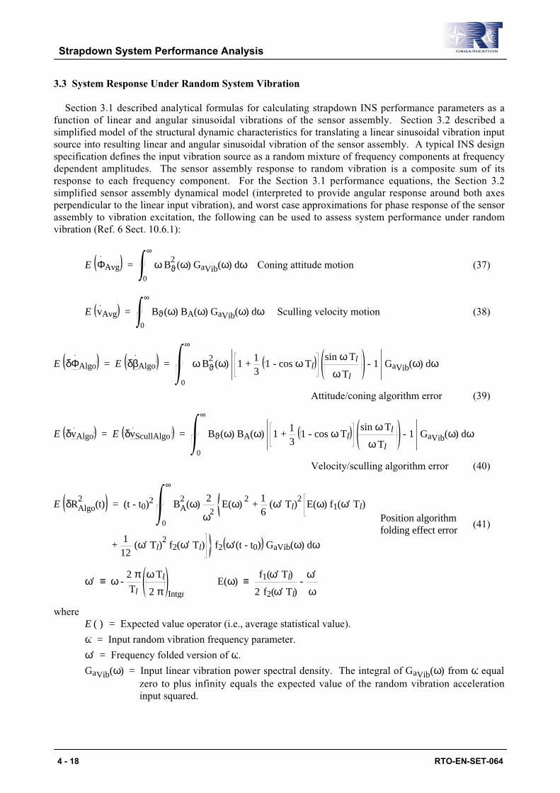
3.3 System Response Under Random System Vibration
Section 3.1 described analytical formulas for calculating strapdown INS performance parameters as a
function of linear and angular sinusoidal vibrations of the sensor assembly. Section 3.2 described a
simplified model of the structural dynamic characteristics for translating a linear sinusoidal vibration input
source into resulting linear and angular sinusoidal vibration of the sensor assembly. A typical INS design
specification defines the input vibration source as a random mixture of frequency components at frequency
dependent amplitudes. The sensor assembly response to random vibration is a composite sum of its
response to each frequency component. For the Section 3.1 performance equations, the Section 3.2
simplified sensor assembly dynamical model (interpreted to provide angular response around both axes
perpendicular to the linear input vibration), and worst case approximations for phase response of the sensor
assembly to vibration excitation, the following can be used to assess system performance under random
vibration (Ref. 6 Sect. 10.6.1):
E ΦAvg = ω Bϑ2
(ω) GaVib(ω) dω0
∞
Coning attitude motion (37)
E vAvg = Bϑ(ω) BA(ω) GaVib(ω) dω0
∞
Sculling velocity motion (38)
E δΦAlgo = E δβAlgo = ω Bϑ2
(ω) 1 + 13
1 - cos ω Tl sin ω Tl
ω Tl
- 1 GaVib(ω) dω
0
∞
Attitude/coning algorithm error (39)
E δvAlgo = E δvScullAlgo = Bϑ(ω) BA(ω) 1 + 13
1 - cos ω Tl sin ω Tl
ω Tl
- 1 GaVib(ω) dω
0
∞
Velocity/sculling algorithm error (40)
E δRAlgo2
(t) = (t - t0)2 BA2
(ω) 2
ω2 E(ω)
2 +
16
(ω′ Tl)2 E(ω) f1(ω′ Tl)
0
∞
+ 1
12 (ω′ Tl)
2 f2(ω′ Tl) f2 ω′(t - t0) GaVib(ω) dω
Position algorithmfolding effect error
(41)
ω′ ≡ ω - 2 πTl
ω Tl
2 π Intgr
E(ω) ≡ f1 (ω′ Tl)
2 f2 (ω′ Tl) -
ω′
ω
where
E ( ) = Expected value operator (i.e., average statistical value).
ω = Input random vibration frequency parameter.
ω′ = Frequency folded version of ω.
GaVib(ω) = Input linear vibration power spectral density. The integral of GaVib(ω) from ω equal
zero to plus infinity equals the expected value of the random vibration acceleration
input squared.
4 - 18 RTO-EN-SET-064

Strapdown System Performance Analysis
The f1, f2 functions, BA(ω) and Bϑ(ω) are defined in Equations (32) and (35). Note that E δRAlgo2
(t) for
the position error is based on the Equation (31) form to avoid singularities when the folded frequency ω′ iszero.
The previous methodology for evaluating particular INS error characteristics under random (and
sinusoidal) vibration can be applied to other INS error effects as well. Reference 6 Sections 10.6.1-10.6.3
provide several examples in addition to those discussed previously.
4. SYSTEM TESTING FOR INERTIAL SENSOR CALIBRATION ERRORS
After an INS (or its sensor assembly) is assembled and sensor compensation software coefficients have
been installed (typically based on sensor calibration measurements), it is frequently required that residual
sensor error parameters be measured to assess system level performance. For compensatable effects, the
results can be used to update the sensor calibration coefficients. This section describes two INS system
level tests that are typically conducted in the laboratory for measuring residual bias, scale-factor and
misalignment errors: the Strapdown Drift Test and the Strapdown Rotation Test. The Strapdown Drift test
is a static test performed on high performance sensor assemblies in which the attitude integration software
in the INS computer is configured to constrain the average horizontal transformed specific force
acceleration to zero. For a test of several hours duration, the averages of the constraining signals become
accurate measures of horizontal angular rate sensor bias error. The Strapdown Rotation Test can be used on
sensor assemblies of all accuracy grades. It consists of exposing the INS to a series of rotations, and
recording its average transformed specific force acceleration output at static dwell times between rotations.
By processing the recorded data, very accurate measurements can be made of the scale factor error and
relative misalignment between all inertial sensors in the sensor assembly, the accelerometer bias errors, and
misalignment of the sensor assembly relative to the INS mounting fixture. The details of these tests and
others are described in Reference 6 Chapter 18.
4.1 Strapdown Drift Test
The Strapdown Drift test is designed to evaluate angular rate sensor error by processing data generated
during extended self-alignment operations. The test is performed on a strapdown analytic platform during
an extension of the normal self-alignment initialization mode. The principal measurement of the Strapdown
Drift Test is the composite north horizontal angular rate sensor output, determined from the north
component of angular rate bias applied to the strapdown analytic platform to render it stationary in tilt
around North. Subtracting the known true value of north earth rate from the measurement evaluates the
north component of angular rate sensor composite error. East and vertical angular rate sensor errors are
ascertained by repeating the test with the previously east and vertical angular rate sensors in the horizontal
north orientation.
The self-alignment process utilized in the Strapdown Drift Test creates a locally level rotation rate
stabilized analytic "platform" (the N Frame) whose level orientation (relative to the earth) is sustained based
on horizontal platform acceleration measurements (i.e., perpendicular to the accelerometer derived local
gravity vertical). The test measurement is the biasing rate to the analytically stable platform to maintain it
level in the presence of earth's rotation. As configured, the analytic platform remains angularly stable in the
presence of B Frame angular rate, hence, angular rate sensor bias determined from stabilized platform
measurements becomes insensitive to small physical angular movements of the sensor assembly during the
test (caused for example by test-fixture/laboratory micro-motion relative to the earth or rotation of the
sensor assembly internal mount (within the INS) due to thermal expansion under thermal exposure testing).
Angular rate sensor bias determined by the previous method is corrupted by angular rate sensor scale
factor and misalignment compensation error residuals which are generally negligible in the Strapdown Drift
RTO-EN-SET-064 4 - 19

Strapdown System Performance Analysis
Test environment compared with typical high accuracy bias accuracy requirements. Also contained in the
bias measurements are the effects of angular rate sensor random output noise which is reduced to an
acceptable level by allowing a long enough extended self-alignment measurement period. If test accuracy
requirements permit, a simpler version of the Strapdown Drift Test can be utilized in which the test
measurement is the direct integral of the compensated angular rate from each sensor minus its earth rate
component input. To reduce earth rate input misalignment error effects using the latter approach, the
angular rate sensor can be oriented with its input axis aligned with earth's polar rotation axis. The simpler
approach is directly susceptible to angular motion of the sensor assembly relative to the earth during the test
measurement.
For situations when the biasing rate to the strapdown analytic platform is not an available INS output, an
alternative procedure can be utilized based on INS computed true heading outputs (Ref. 6 Sect. 18.2.2). In
this case the east angular rate sensor error is determined from the test based on the heading error it generates
at the end of an extended self-alignment run. In order to discriminate east angular rate sensor error from
North earth rate coupling (under test heading misalignment), the INS heading output is measured for two
individual alignment runs. The second alignment run is performed at a heading orientation that is rotated
180 degrees from the first. The difference between the average heading measurements so obtained cancels
the North earth rate coupling input, thereby becoming the measurement for east angular rate sensor error
determination. North and vertical angular rate sensor errors are ascertained by repeating the test with the
previously north and vertical angular rate sensors in the horizontal east orientation.
The following operations are integrated to implement the strapdown analytic platform function during the
Strapdown Drift Test extended alignment computational process (Ref. 6 Sect. 6.1.2):
CBN
= CBN
ωIBB
× - ωINN
× CBN
ωINN
= ωIEN
+ ωTiltN
ωTiltN
= K2 uUpN
× ∆RHN
ωIEN
= ωIEH
N + uUp
N ωe sin l (42)
ωIEH
N = K1 uUp
N × ∆RH
N
vHN
= CBN
H aSF
B - K3 ∆RH
N
∆RHN
= vHN
- K4 ∆RHN
where
ωIBB
, aSFB
= Angular rate sensor and accelerometer compensated input vectors.
H = Subscript indicating horizontal components (or rows)of the associated vector (or matrix).
Ki = Extended alignment analytical platform level maintenance coefficients.
ωe = Earth inertial rotation rate magnitude.
l = Geodetic latitude.
uUp = Unit vector upward along the geodetic vertical (i.e., along the N Frame Z axis).
v, ∆R = Velocity and position displacement during extended alignment.
The North angular rate sensor bias is calculated as an adjunct to the previous operations as (Ref. 6 Sect.
18.2.1):
φHN
≡ ωINH
N dt
tStart
tEnd
δωARS/CnstNorth ≈ 1
tEnd - tStart φH - ωe cos l (43)
4 - 20 RTO-EN-SET-064

Strapdown System Performance Analysis
where
tStart, tEnd = Time at the start and end of the Strapdown Drift Test measurement period.
δωARS/CnstNorth = North component of angular rate sensor constant bias residual error.
ωe = Earth rotation rate magnitude.
l = Test site latitude.
φH = Magnitude of φH.
4.2 Strapdown Rotation Test
The basic concept for the Strapdown Rotation Test was originally published by the author in 1977
(Reference 3). Since then, variations of the concept have formed the basis in most strapdown inertial
navigation system manufacturing organizations for system level calibration of accelerometer/angular-rate-
sensor scale-factors/misalignments and accelerometer biases.
The Strapdown Rotation test consists of a series of rotations of the strapdown sensor assembly using a
rotation test fixture for execution. During the test, special software operates on the strapdown angular rate
sensor outputs from the sensor assembly to form an analytic angular rate stabilized wander azimuth
"platform" (L Frame - See definition to follow) that nominally maintains a constant orientation relative to
the earth. The analytic platform is implemented by processing strapdown attitude-integration/acceleration-
transformation algorithms (e.g., Reference 7 Equations (8), (12), (14), (24) and (26) including inertial sensor
compensation Equations (38)) with the platform horizontal inertial rotation rate components held constant.
Platform horizontal rotation rates are calculated prior to rotation test initiation using special test software
that implements strapdown initial alignment algorithms (e.g., Equations (42) using Kalman filter formulated
Ki gains). Measurements during the Strapdown Rotation test are taken at stationary positions and computed
from the averaged transformed accelerometer outputs plus gravity (i.e., the average computed total
acceleration vector):
∆vmL
≡ aSFL
+ gL dttm-1
tm
= ∆vSFm
L - gTst uUp
L Tm
∆vSFm
L ≡ CB
L aSF
B dt
tm-1
tm
(44)
aL = abc
≈ 1
Tm ∆vAvg
LTest measurements
where
L Frame = "Attitude Reference" coordinate frame aligned with the N Frame but having Z axis
parallel to the downward (rather than upward) vertical and with X, Y axes interchanged
(the L Frame X, Y axes are parallel to the N Frame Y, X axes). Reference 6 uses the L
Frame for "attitude reference" outputs as an intermediate frame between the B and N
Frames.
g = Plumb-bob gravity vector at the test site (mass attraction "gravitation" plus earth rotation effect
centripetal acceleration).
gTst = Vertical component of g.
∆vAvgL
= Output from an averaging process performed on successive ∆vSFm
L's (See Reference 6
Section 18.4.7.3 for process designed to attenuate accelerometer quantization noise).
a = Average total acceleration.
a, b, c = Components of a in the L Frame.
RTO-EN-SET-064 4 - 21

Strapdown System Performance Analysis
The fundamental theory behind the Strapdown Rotation test is based on the principle that for a perfectly
calibrated sensor assembly, following a perfect initial alignment, the computed L Frame acceleration should
be zero at any time the sensor assembly is stationary. Moreover, this should also be the case if the sensor
assembly undergoes arbitrary rotations between the time periods that it is set stationary. Therefore, any
deviation from zero stationary acceleration can be attributed to imperfections in the sensor assembly (i.e.,
sensor calibration errors) or in the initial alignment process. Initial alignment process errors create initial L
Frame tilt which is removed from the Strapdown Rotation Test measurements by structuring the horizontal
measurements as the difference between average horizontal L Frame acceleration readings taken before and
after completing each of the test rotation sequences. As an aside, it is to be noted that in the original
Reference 3 paper, the measurement for the rotation test was the average acceleration taken at the end of
each rotation sequence, with a self-alignment performed before the start of each rotation sequence. The
purpose of the realignment was to eliminate attitude error build-up caused by angular rate sensor error
during previous rotation sequences. By taking the measurement as the difference between average
accelerations before and after rotation sequence execution (as indicated above), the need for realignment is
eliminated. The before/after measurement approach was introduced by Downs in Reference 1 forcompatibility with an existing Kalman filter used to extract the acceleration measurements.
The principal advantage for this particular method of error determination derives from the combined use
of the angular rate sensors and accelerometers to establish an angular rate stabilized reference for measuring
accelerations. This implicitly enables the inertial sensors to measure the attitude of the rotation test fixture
settings as the rotations are executed. Consequently, precision rotation test table readout or controls are not
required (nor a stable test fixture base), hence, a significant savings can be made in test fixture cost.
Inaccuracies in rotation fixture settings manifest themselves as second order errors in sensor error
determination, which can be made negligibly small if desired through a repeated test sequence. It has been
demonstrated, for example, with precision ring laser gyro strapdown inertial navigation systems, that the
test method can measure and calibrate gyro misalignments to better than 1 arc sec accuracy with 0.1 deg
rotation fixture orientation inaccuracies. In addition, because the orientation of the sensor assembly is being
measured by the sensor assembly itself, it is not necessary that the sensor assembly be rigidly connected to
the rotation test fixture. This is an important advantage for high accuracy applications in which the sensor
assembly is attached to its chassis and mounting bracket through elastomeric isolators of marginal attitude
stability.
While most of the sensor calibration errors evaluated by the Strapdown Rotation test can be measured
on an individual sensor basis, the rotation test is the only direct method for measuring relative
misalignments between the sensor input axes. It should also be noted that determination of sensor-
assembly-to-mount misalignment is not an intrinsic part of the Strapdown Rotation Test, however, because
the data taken during the test allows for this determination, it is easily included as part of test data
processing (Ref. 6 Sect. 18.4.5).
Reference 6 Section 18.4 (and subsections) provides a detailed description of the Strapdown Rotation
Test, its analytical theory, processing routines, and structure based on two sets of rotation sequences (a 16
rotation sequence set and a 21 rotation sequence set). The rotation sequences for the 16 set are summarized
in Table 1.
4 - 22 RTO-EN-SET-064

Strapdown System Performance Analysis
Table 1 - 16 Set Rotation Test Sequences
SEQUENCE
NUMBER
ROTATION SEQUENCE
(Degrees, B Frame Axis)
STARTING ATTITUDE
(+Z Down, Axis Indicated
Along Outer Rotation
Fixture Axis)
1 +360 Y +Y
2 +360 X +X
3 + 90 Y, +360 Z, - 90 Y +Y
4 +180 Y, + 90 Z, +180 X, - 90 Z +Y
5 +180 X, + 90 Z, +180 Y, - 90 Z +X
6 + 90 Y, + 90 Z, - 90 X, - 90 Z +Y
7 + 90 Y +Y
8 - 90 Y +Y
9 + 90 Y, + 90 Z +Y
10 + 90 Y, - 90 Z +Y
11 - 90 Y, - 90 Z +Y
12 + 90 X, + 90 Z +X
13 + 90 X, - 90 Z +X
14 +180 Z +Y
15 +180 Y +Y
16 +180 X +X
RTO-EN-SET-064 4 - 23

Strapdown System Performance Analysis
Based on the Table 1 rotation sequences, Reference 6 Section 18.4.3 develops the relationship between
the test measurements and the sensor errors excited by the test; e.g., for Table 1 rotation sequences 1 and 9:
∆a1 = - 2 π g κyy
∆b1 = 0
c11 = c1
2 = - g λzz - λzzz + αz
∆a9 = - g 12
υzx + 12
υyz + µzy - µxz + π2
κyy
- αx + αz
∆b9 = g 12
υxy + 12
υyz + µyz - µxy + π2
κzz
+ αx - αy
c91 = - g λzz - λzzz + αz
c92 = - g λyy - λyyy + αy
(45)
where
∆ai, ∆bi = Difference between a, b horizontal acceleration measurements taken at the start and endof rotation sequence i.
ci1, ci
2 = Vertical acceleration measurements taken immediately before (superscript 1) and after
(superscript 2) rotation sequence i.
α i = i axis accelerometer bias calibration error.
λ ii = i axis accelerometer symmetrical scale factor calibration error.
λ iii = i axis accelerometer scale factor asymmetry calibration error.
κ ii = i axis angular rate sensor scale factor calibration error.
υij = Orthogonality compensation error between the i and j angular rate sensor input axes, defined
as π/2 radians minus the angle between the compensated i and j sensor input axes.
µij = i axis accelerometer misalignment calibration error, coupling specific force from the j axis ofthe mean angular rate sensor axes into the i axis accelerometer input axis.
The mean angular rate sensor (MARS) axis frame in the previous µij definition refers to a B Frame definedas the orthogonal triad that best fits symmetrically within the actual compensated angular rate sensor inputaxes. The “best fit” condition is specified as the condition (measured around angular rate sensor axis k) forwhich the angle between angular rate sensor input axis i and MARS axis i equals the angle between angularrate sensor input axis j and MARS axis j (Ref. 6 Sect. 18.4.3). As such, the overall angular misalignment ofthe actual angular rate sensor triad is defined to be zero relative to the MARS frame, and individual angularrate sensor misalignments affecting the Strapdown Rotation Test measurements are only due toorthogonality errors between the angular rate sensor axes.
Once the ∆ai, ∆bi, ci1, ci
2 measurements are obtained, the individual sensor residual errors can be
calculated deterministically as summarized in Figure 4 (Ref. 6 Sect. 18.4.4). The results so obtained can
then be used to update the INS sensor calibration coefficients (Ref. 6 Sect. 18.4.6). If the B Frame is
chosen to be the MARS Frame as described previously, the µij accelerometer misalignments calculated
from Figure 4 would be used directly to update the accelerometer misalignment calibration coefficients
relative to the B Frame. For the angular rate sensors, selecting the B Frame as the MARS Frame equates to
the following for individual angular rate sensor misalignments relative to the B Frame as:
κxy = κyx = 12
υxy κyz = κzy = 12
υyz κzx = κxz = 12
υzx (46)
where
κ ij = Angular rate sensor misalignment calibration error coupling B Frame j axis angular rate intothe i angular rate sensor input axis.
4 - 24 RTO-EN-SET-064

Strapdown System Performance Analysis
ANGULAR RATE SENSOR CALIBRATION ERRORS
Scale Factor Errors Orthogonality Errors
κxx = - 1
2 π g ∆a2
κyy = - 1
2 π g ∆a1
κzz =1
2 π g ∆b3
υxy =1g
∆b6 - 12
∆b4 - 14
∆b3
υyz =1
4 g ∆b5 + ∆b4
υzx =1
4 g ∆b5 - ∆b4
ACCELEROMETER CALIBRATION ERRORS
Bias Errors Scale Factor Errors
αx = 14
∆a1 - 12
∆a15
αy = 12
∆a16 - 14
∆a2
αz = 12
∆a7 - ∆a8 - 14
∆a1
λxx = - 1
2 g c12
2 + c13
2
λyy = - 1
2 g c9
2 + c10
2
λzz = - 1
2 g c14
2 + c15
2
Misalignment Errors Relative To
Scale Factor Asymmetry Mean Angular Rate Sensor Axes
λxxx =1
2 g c12
2 - c13
2 + ∆a15 -
12
∆a1
λyyy =1
2 g c9
2 - c10
2 - ∆a16 +
12
∆a2
λzzz =1
2 g c14
2 - c15
2 - ∆a7 + ∆a8 +
12
∆a1
µxy =1
2 g ∆b11 - ∆b10 + ∆b6 -
34
∆b3 - 12
∆b4
µyx =1
2 g ∆b7 - ∆b8 - ∆b6 +
12
∆b4 + 14
∆b3
µyz =1
2 g ∆b14 + ∆a16 -
12
∆a2 + 14
∆b4 + 14
∆b5
µzy =1
2 g ∆a10 - ∆a9 -
14
∆b4 - 14
∆b5
µzx =1
2 g ∆a13 - ∆a12 -
14
∆b5 + 14
∆b4
µxz =1
2 g ∆a14 - ∆a15 +
12
∆a1 + 14
∆b5 - 14
∆b4
Figure 4 - Sensor Errors In Terms Of MeasurementsFor The 16 Rotation Sequence Test
RTO-EN-SET-064 4 - 25

Strapdown System Performance Analysis
5. SYSTEM PERFORMANCE ANALYSIS
To assess the accuracy of inertial navigation systems, error analysis techniques are traditionally
employed in which error equations are used to describe the propagation of system navigation error
parameters in response to system error sources. The error equations also form the basis for performance
improvement techniques in which the inertial system errors are estimated and controlled in real time based
on navigation measurements taken from other navigation devices (e.g., GPS satellite range measurements).
Such "aided" inertial navigation systems are structured using a Kalman filter in which system error
estimates are based on a running statistical determination of the expected instantaneous errors (e.g.,
typically in the form of a "covariance matrix"). The covariance matrix computational structure used in the
Kalman filter is also applied in "covariance analysis" simulators to statistically analyze both aided and
unaided ("free inertial") system performance. Validation of the Kalman filter software is an important
element in the aided inertial navigation system software design process.
5.1 Free Inertial Performance Analysis
The accuracy of all inertial navigation systems is fundamentally limited by instabilities in the inertial
component error characteristics following calibration. Resulting residual inertial sensor errors produce INS
navigation errors that are unacceptable in many applications. To predict Strapdown INS performance,
linear time rate differential error propagation equations can be analyzed depicting the growth in INS
computed attitude, velocity, position error as a function of residual inertial sensor and gravity modeling
error (e.g., Ref. 7 Eqs. (50)). Modern formulations of such error propagation equations cast them in a
standard error state dynamic equation format as follows (Ref. 2 Sect. 3.1 and Ref. 6 Sect. 15.1):
x(t) = A(t) x(t) + GP(t) nP(t) (47)
where
x(t) = Error state vector treated analytically as a column matrix.
A(t) = Error state dynamic matrix.
nP(t) = Vector of independent white “process” spectral noise density sources driving x(t) (treated
analytically as a column matrix).
GP(t) = Process noise dynamic coupling matrix that couples individual nP(t) components into x(t) .
In general, A(t) and GP(t) are time varying functions of the angular rate, acceleration, attitude, velocity
and position parameters within the INS computer. To evaluate the solution to Equation (47) at discrete time
instants, the following equivalent integrated form is utilized (Ref. 2 Sect. 3.4 and Ref. 6 Sect. 15.1.1):
xn = Φn xn-1 + wn (48)
in which
Φ(t, tn-1) = I + A(τ) Φ(τ, tn-1) dτtn-1
t
Φn ≡ Φ(tn, tn-1) (49)
wn = Φ(tn,τ) GP(τ) nP(τ) dτtn-1
tn
(50)
where
n = Performance evaluation cycle time index.
xn = Error state vector evaluated at cycle time n.
Φn = Error state transition matrix that propagates the error state vector from the n-1th to the nth
time instant.
4 - 26 RTO-EN-SET-064

Strapdown System Performance Analysis
wn = Change in xn due to process noise input from the n-1th to the nth time instant.
For a strapdown INS, the elements of the x error state vector would include INS attitude, velocity, position
error parameters, inertial sensor error parameters (e.g., bias, scale factor, misalignment) and gravity
modeling error. Elements of the nP process noise vector would include inertial sensor random output noise,
noise source input to randomly varying inertial sensor error states, and noise source inputs to randomly
varying gravity error modeling error states. Equations (50) of Reference 7 are an example of strapdown
INS error propagation equations that are in the Equation (47) form. The sensor error terms in these
equations are typically modeled as random constants (with random walk input white noise), first order
Markov processes, or the sum of both (Ref. 6 Sect. 12.5.6). Reference 6 Section 16.2.3.3 provides an
example of how the gravity error term in these equations can be modeled.
5.2 Kalman Filters For INS Aiding
To overcome the performance deficiencies in a free inertial navigation system, “inertial aiding” is
commonly utilized in which the INS navigation parameters (and in some cases, the sensor calibration
coefficients) are updated based on inputs from an alternate source of navigation information available in the
user vehicle. The modern method for applying the inertial aiding measurement to the INS data is through a
Kalman filter, a set of software that is typically resident in the INS computer. The Kalman filter is designed
based on the Equation (48) x error state vector propagation model, to generate estimates for x and provide
updates to the INS computer parameters to control x (ideally to zero). For an aided INS, the x error state
vector would also include error terms associated with the aiding device. The basic structure of a real-time
Kalman filter based on "delayed control resets" (to allow for finite computation time delay - Ref. 6 Sect.
15.1.2) is:
ξINS n(+c) = ξINS n(-) + gINS ξINS n(-), uc n
ξAid n(+c) = ξAid n(-) + gAid ξINS n(-), uc n
(51)
ZObs n = f ξINSn(+c), ξAidn(+c) (52)
xn(-) = Φn xn-1(+e) (53)
xn(+c) = xn(-) + uc n (54)
zn = Hn xn(+c) (55)
xn(+e) = xn(+c) + Kn ZObsn - zn (56)
uc n+1 = function of xn(+e) (57)
x0 = 0 Initial Conditions (58)
where
ξINS = INS navigation parameters.
ξAid = Aiding device navigation parameters.
gINS( ), gAid( ) = Non-linear functional operators used to apply uc n to the ξINS, ξAid navigation
parameters at time tn such that the error in these parameters is controlled
(typically to zero).
RTO-EN-SET-064 4 - 27

Strapdown System Performance Analysis
f ( ) = Functional operator that compares designated equivalent elements of ξ INS and ξAid . The
f( ) operator is designed so that for an error free INS, an error free aiding device, and a
perfect (error free) f ( ) software implementation, f ( ) will be zero.
ZObs = Observation vector formed from the comparison between comparable INS and aiding
device navigation parameters.
uc n+1 = Control vector derived from the Kalman filter estimate of the time tn value of x and applied
at time tn+1 to constrain the actual value of x.
= Value for parameter estimated (or predicted) by the Kalman filter.
(+e) = Designation for parameter value at its designated time stamp (tn in this case) immediately
after (“a posteriori”) the application of estimation resets (e subscript) at the same designated
time.
(+c) = Designation for parameter value at its designated time stamp (tn in this case) immediately
after (“a posteriori”) the application of control resets (c subscript) at the same designated
time.
(-) = Designation for parameter value at its designated time stamp (tn in this case) immediately
prior to (“a priori”) the application of any resets (estimation or control) at the same designated
time.
Kn = Errors state estimation gain matrix.
n = Kalman filter software cycle time index.
n = at the nth Kalman filter cycle time.
z = Estimated "measurement vector" analytically represented as a column matrix. The z equation
implemented in the Kalman filter represents a linearized version of the ZObs observation
equation based on the expected (projected) value of the error state vector x when ZObs is
measured.
H = The "measurement matrix". Generally a time varying function of the navigation parameters
calculated in the INS computer. See further description in the paragraph following Equation
(59) parameter definitions.
The previous Latin notation “a priori” and “a posteriori” has been adopted in Kalman filter terminology to
add an element of “mysterioso”. Identification of individual (+e) and (+c) “a posteriori” updates provides
flexibility to allow for different Kalman filter estimation/control time points (e.g., for timing and
synchronization of observation/measurement/control operations - Ref. 6 Sect. 15.1.2.4).
The estimation process described by Equation (56) is general and becomes a Kalman filter operation
when the gain matrix Kn matrix is computed based on “optimally” estimating the error state vector as
follows (Ref. 2 Sect. 4.2 and Ref. 6 Sect. 15.1.2.1):
K n = Pn(-) HnT
Hn Pn(-) HnT
+ GM n Rn GM n
T -1 (59)
in which
P ≡ E ∆x ∆xT ∆x ≡ x - x Rn ≡ E nMn nMn
T
where
∆x = Error state vector estimation uncertainty.
P = Error state vector uncertainty covariance matrix.
nM = Vector of independent white measurement noise sources (represented analytically as a
column matrix). The nM vector represents noise type error effects that may be introduced in
the process of making the ZObs observation.
4 - 28 RTO-EN-SET-064

Strapdown System Performance Analysis
GM = Measurement noise dynamic coupling matrix that couples nM into the ZObs observation.
Generally a time varying function of the navigation parameters calculated in the INS
computer.
From an analytical standpoint, GM and nM in Equation (59) (and H in Equation (55)) are defined as part of
z , the linearized analytical form of the ZObs observation, which is denoted as the "measurement equation":
zn = Hn xn + GMn nMn (Ref. 6 Sect. 15.1 and Ref. 2 Sect. 3.5). The covariance matrix P in Equation (59)
is calculated by an integration operation based on the statistical uncertainty in the Equation (56) estimation
process (using the previous zn approximation for ZObs n) and the Equation (53) approximation for the actual
Equation (48) error state vector propagation between estimation cycles (Ref. 2 Sect. 4.2 and Ref. 6 Sects.
15.1.2.1 and 15.1.2.1.1):
Pn(-) = Φn Pn-1(+e) ΦnT
+ Qn (60)
Pn(+e) = I - K n Hn Pn(-) I - K n HnT + K n GM n Rn GM n
T K n
T (61)
in which
Qn ≡ E wn wnT
5.2.1 Covariance Simulation Analysis
The computational structure used in computing the Kalman filter covariance matrix (Eqs. (59) - (61)) can
also be used in performance analysis time domain simulation programs for statistically estimating aided
INS accuracy (or unaided performance by setting the Kn gain matrix to zero). Such covariance simulation
programs (Ref. 6 Chpt. 16) are commonly used to provide numerical time histories depicting the accuracy
of a given system configuration in terms of the covariance of its associated linearized error state vector. For
a Kalman filter aided system, the covariance simulation is also utilized as a basic design tool during the
synthesis and test of the "suboptimal" Kalman filter configuration used in the actual system. The
suboptimal Kalman filter configuration is typically based on a simplified error state dynamic/measurement
model (compared to the “real world” error state dynamics/measurements) with numerical values for its
defining matrix elements that may differ from real world values. The covariance simulation is used to
evaluate the performance of the suboptimal filter operating in a real world environment, and to provide the
design engineer with useful sensitivities for identifying sources of undesirable performance characteristics
during the design process.
5.3 Kalman Filter Validation
Although a Kalman filter is generally a complex software package, its validation process can be fairly
straight-forward because of its fundamental underlying structure. The Kalman filter elements are well
defined analytically and can be validated individually based on their intrinsic properties. Once the elements
are validated, the proper operation of the filter is assured through its theoretical structure.
As an example, Reference 6 Section 15.1.4 discusses the following operations that can be performed
using specialized test simulators for validating the Equations (51) - (58) and (59) - (61) Kalman filter
algorithms:
• The state transition matrix Φn, estimated measurement zn, and observation ZObsn algorithms can be
validated by operating Equations (51) - (58) “open loop” (i.e., setting the Kalman gain Kn and
RTO-EN-SET-064 4 - 29

Strapdown System Performance Analysis
control vector u c to zero) using simulators for ξ INSn and ξAidn
. The ξ INSn simulator would consist
of the strapdown inertial navigation algorithms upon which Φn is based. The ξAidn simulator would
be built onto a previously validated trajectory generator; the trajectory generator would also provide
the strapdown inertial sensor inputs to ξ INSn . The Kalman filter error state vector xn components
would be initialized to some arbitrary non-zero value; the same error values would be inserted into
the ξ INSn , ξAidn
parameters. Under these conditions, the Kalman filter estimated measurement zn
calculated with (55) should track the observation vector ZObsn computed with (52), resulting in a
zero value for the measurement residual ZObsn - zn (within the fundamental linearization error in zn).
A zero measurement residual validates the Φn, zn and ZObsn algorithms and associated timing
structure in the simulation implementation.
• The covariance propagation algorithm (with process noise set to zero) can be validated as part of the
previous process by initially setting the covariance matrix equal to the arbitrarily defined xn error
state vector times its transpose. The covariance matrix would then be propagated without resets
using the Equation (60) algorithm or a Reference 6 Section 15.1.2.1.1.3 equivalent (several
propagation cycles between estimation cycles). The propagated covariance matrix should then equal
the propagated error state vector times its transpose.
• The algorithms for calculating the Kalman gain matrix Kn and resetting the covariance matrix can be
validated by comparing the covariance reset algorithm output with the output from an equivalent
alternative algorithm based on the analytical form of Kn (e.g., the Equation (61) "Joseph’s" form
compared with the Reference 6 Equation (15.1.2.1.1-4) optimal form). The results should be
identical.
• The basic estimation capability of the Kalman filter can be validated by disabling the control vector
(setting uc to zero) and allowing the Kalman filter to estimate xn in the presence of selected values
for the error state components initially imbedded in ξ INSn and ξAidn . For this test, the process and
measurement noise matrices in the Kalman filter covariance propagation/reset routines would be set
to zero to heighten sensitivity (and better account for the error condition being simulated).
• Kalman filter estimation capability in the presence of process and measurement noise can be
validated by repeating the previous test, but with random noise (from a software noise generator at
the Kalman filter specified white noise source amplitudes) applied appropriately to the ξ INSn , ξAidn
models (for process noise) and to the ZObsn routine (for measurement noise). The Kalman filter
process and measurement noise matrices would also be active for this test. In parallel, a “truth
model” error state vector history would be generated using the same noise and initial conditions
applied to a simulated version of error state dynamic Equation (47). The uncertainty in the Kalman
filter estimated error state vector is evaluated by comparing the filter error state vector estimate with
the “truth model” error state vector. Repeated runs with different random noise generator initial
“seeds” provides an ensemble history of the error state uncertainty. The ensemble average of the
uncertainty times its transpose (at common time points) should match the corresponding filter
covariance matrix history.
• The control vector uc interface in control reset Equations (51) and (54) can be validated by assigning
an arbitrary value to uc and applying it to the previous equations. If the control reset equations and
the measurement/observation algorithms are consistent, the measurement residual ZObsn - zn should
be unaffected by the control reset application.
4 - 30 RTO-EN-SET-064

Strapdown System Performance Analysis
A previously validated trajectory generator is an important supporting software element in the Kalman
filter validation process to provide truth model navigation parameter data over a user shaped trajectory
profile. A trajectory generator is also required in covariance analysis programs to provide navigational
parameters for computing the error-state-transition, measurement and noise matrices. Reference 6 Chapter
17 describes a trajectory generator based on exact strapdown inertial navigation integration algorithms that
can be validated using the steps outlined in Section 2 (and subsections) of this paper.
6. SYSTEM INTEGRATION TESTING
System performance testing is conducted to verify that the system meets accuracy requirements under
anticipated user environments (e.g., temperature, vibration, altitude, etc.). Prior to performance testing,
system integration testing must be conducted to verify that functional operations are performed properly and
accurately by all hardware, software, and interface elements. Based on direct experience, it is the author's
firm contention that all software operations should be (and can be) completely validated prior to
hardware/software integration of a strapdown INS. Otherwise, problems that will inevitably be encountered
during final system integration (e.g., software errors due to programming flaws or algorithm error) may
never be completely resolved (e.g., hardware designers may fault the software, software designers may fault
the hardware - particularly the inertial components, thus discouraging meaningful problem resolution). For
an aided strapdown INS, the software validation procedures discussed in Sections 2 and 5.3 can be utilized.
Hardware/software integration begins with software/system-computer integration. The purpose should
be to verify identical performance in the system computer (within minuscule round-off error) as achieved in
the computer used for software validation. Toward this end, the same simulators/truth-models used for the
software validation process would be installed with the system software being integrated as the
computer/software integration test driver/evaluator. The driver/evaluator should be designed/validated (as
part of the software validation process) to fully exercise/verify all system software under simulated system
inputs. In this regard, the driver/evaluator should be considered to be an integral part of the validated
system software. For today's computer technology with associated high speed floating point architecture,
long word-length, large memory capabilities and abundant software compiler/translator tools,
computer/software integration should be a fairly straightforward task.
Hardware integration precedes hardware/software integration based on traditional methods in which
functional elements are first individually tested, then interfaced/tested in functional groups until a fully
integrated hardware assembly is verified. A critical part of hardware integration is the individual testing (by
applied stimulus) of all functional element input/output interfaces to verify that proper signals are being
transmitted to assigned locations with proper phasing. Analog signal inputs to the system computer must be
individually tested to assure proper error free analog-to-digital conversion. Digital computer interfaces
should be individually checked to assure immunity to system self-generated electrical noise and externally
applied electro-magnetic interference (EMI). For a strapdown INS, common internal computer interfaces to
be tested are for inertial sensor inputs, for individual temperature probe inputs (used for temperature
sensitive sensor compensation software), and for special computer input/output signals used to control
individual internal sensor operations (e.g., path length control resets for ring laser gyros). Successful
interface testing requires pre-planning in the hardware design process for the ability to stimulate all
interfaces to be tested. For an aided INS, interfaces with the aiding device must also be verified (e.g., GPS
data).
A powerful technique for demonstrating satisfactory completion of the strapdown INS hardware/software
integration process is to execute a system level laboratory calibration procedure (e.g., using the Section 4.1
and 4.2 Strapdown Rotation Test and Strapdown Drift Test). The system should perform accurately after
re-calibration based on the test results. For a GPS aided INS, a successful GPS data interface can be
demonstrated by a correct GPS data based position solution generated independently within the integrated
system computer (compared with the same solution generated externally using an independent GPS receiver
system).
RTO-EN-SET-064 4 - 31

Strapdown System Performance Analysis
For recent GPS aided INS micro-electronic "deeply integrated" architectures designed around MEMS
(micro-machined electro-mechanical systems) inertial sensors, application of the previous integration test
techniques poses new challenges.
7. CONCLUDING REMARKS
Strapdown inertial navigation computation algorithms can be accurately validated using simple closed-
form exact solution truth models for reference. Algorithm validation can be greatly facilitated by
structuring the algorithms based on exact integral solutions between update cycles of the continuous form
navigation parameter time rate differential equations. This permits the algorithms to be validated using
simple generic application independent truth models designed to exercise all algorithm elements. The truth
models generally do not have to simulate realistic trajectory profiles.
Vibration induced inertial system error effects are easily analyzed using simplified analytical INS
structural dynamic models. Simplified simulators based on these models can quickly generate numerical
system performance measurements (e.g., coning/sculling motion, coning/sculling algorithm error, position
integration algorithm folding effect error, vibration induced sensor error) as a function of system vibration
power spectrum input, sensor assembly mounting dynamics/imbalance, and algorithm update frequency.
Several methods are available for INS system level performance analysis in the test laboratory to evaluate
residual sensor errors remaining after system calibration. The Strapdown Drift Test and Strapdown
Rotation Test provide simple methods for accurately measuring residual strapdown inertial sensor
calibration errors without requiring elaborate precision test fixturing.
Kalman filters for strapdown INS aiding should be validated based on their natural internal structure
using a simulated version of the INS being aided (interfaced to the Kalman filter) and a simulated aiding
device. The software in the simulated INS should be validated prior to Kalman filter testing. Inputs to the
INS and aiding device simulators would be provided by a previously validated trajectory generator. A
trajectory generator is also required for covariance simulation analysis performance assessment of aided and
unaided inertial navigation systems. Trajectory generator validation can be performed using the same
methods used to validate the INS software.
System software should be thoroughly validated prior to system integration testing.
REFERENCES
1. Downs, H. B., “A Lab Test To Find The Major Error Sources In A Laser Strapdown Inertial Navigator”,38th Annual Meeting of the ION, Colorado Springs, CO, June 15-17, 1982.
2. Gelb, A., Applied Optimal Estimation, The MIT Press, Cambridge Mass., London, England, 1978.
3. Savage, P. G., “Calibration Procedures For Laser Gyro Strapdown Inertial Navigation Systems”, 9th
Annual Electro-Optics / Laser Conference and Exhibition, Anaheim, California, October 25-27,1977.
4. Savage, P. G., “Strapdown Inertial Navigation System Integration Algorithm Design Part 1 - AttitudeAlgorithms”, AIAA Journal Of Guidance, Control, And Dynamics, Vol. 21, No. 1, January-February1998, pp. 19-28.
5. Savage, P. G., “Strapdown Inertial Navigation System Integration Algorithm Design Part 2 - Velocityand Position Algorithms”, AIAA Journal Of Guidance, Control, And Dynamics, Vol. 21, No. 2,March-April 1998, pp. 208-221.
4 - 32 RTO-EN-SET-064

Strapdown System Performance Analysis
6. Savage, P. G., Strapdown Analytics, Strapdown Associates, Inc., Maple Plain, Minnesota, 2000
7. Savage, P. G., "Strapdown System Computational Elements", Advances In Navigation Sensors andIntegration Technology, NATO RTO Lecture Series No. 232, October 2003, Section 3.
RTO-EN-SET-064 4 - 33

Strapdown System Performance Analysis
4 - 34 RTO-EN-SET-064
Recommended