ECE4520/5520: Multivariable Control Systems I. 2–1
STATE-SPACE DYNAMIC SYSTEMS
(CONTINUOUS-TIME)
2.1: Introduction to LTI state-space models
1. What are they?
2. Why use them?
3. How are they related to the transfer
functions we have used already?
4. How do we formulate them?
What are they?
■ Representation of dynamics of an
nth-order system as a first-order
differential equation in an n-vector called
the state ➠ n first-order equations.
“Nice artwork kiddo. I have a feeling
that a great many people will make
a living off that third line someday!”
(Out of Control , IEEE Control Sys-
tems Magazine)
■ Classic example: 2nd-order equation of motion (EOM).
m u.t/
y.t/
k
b
m Ry.t/ D u.t/ ! b Py.t/ ! ky.t/
➠ Ry.t/ Du.t/ ! b Py.t/ ! ky.t/
m:
■ Define a state vector:
x.t/ D
"
y.t/
Py.t/
#
then; Px.t/ D
"
Py.t/
Ry.t/
#
D
2
4
Py.t/
!k
my.t/ !
b
mPy.t/ C
1
mu.t/
3
5 :
Lecture notes prepared by Dr. Gregory L. Plett. Copyright c" 2015, 2011, 2009, 2007, 2005, 2003, 2001, 2000, Gregory L. Plett

ECE4520/5520, STATE-SPACE DYNAMIC SYSTEMS—CONTINUOUS-TIME 2–2
■ We can write this in the form Px.t/ D Ax.t/ C Bu.t/, where A and B
are constant matrices:
Px.t/ D
"
Py.t/
Ry.t/
#
D
2
4
3
5
„ ƒ‚ …
A
"
y.t/
Py.t/
#
C
2
4
3
5
„ ƒ‚ …
B
u.t/:
■ Complete picture by finding y.t/ as function of x.t/: General form is
y.t/ D Cx.t/ C Du.t/;
where C and D are constant matrices:
C Dh i
; D Dh i
:
■ Fundamental form for LTI state-space model:
Px.t/ D Ax.t/ C Bu.t/
y.t/ D Cx.t/ C Du.t/;
where u.t/ is the input, x.t/ is the “state”, A, B, C , D are constant
matrices.
DEFINITION: The state of a system at time t0 is the minimum amount of
information at t0 that, together with the input u.t/, t # t0, uniquely
determines the behavior of the system for all t # t0.
■ Contrast with impulse-response (convolution) representation which
requires all past history of u.t/
y.t/ DZ t
0
h.!/u.t ! !/ d!:
Why use them?
■ Transfer functions provide input-output mapping: u ! G.s/ ! y.
State variables provide access to what is going on inside the system.
Lecture notes prepared by Dr. Gregory L. Plett. Copyright c" 2015, 2011, 2009, 2007, 2005, 2003, 2001, 2000, Gregory L. Plett
ECE4520/5520, STATE-SPACE DYNAMIC SYSTEMS—CONTINUOUS-TIME 2–3
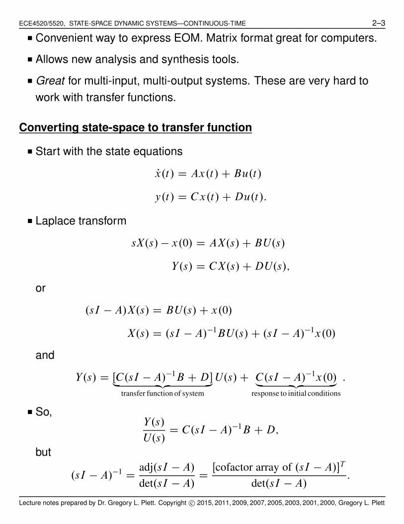
■ Convenient way to express EOM. Matrix format great for computers.
■ Allows new analysis and synthesis tools.
■ Great for multi-input, multi-output systems. These are very hard to
work with transfer functions.
Converting state-space to transfer function
■ Start with the state equations
Px.t/ D Ax.t/ C Bu.t/
y.t/ D Cx.t/ C Du.t/:
■ Laplace transform
sX.s/ ! x.0/ D AX.s/ C BU.s/
Y.s/ D CX.s/ C DU.s/;
or
.sI ! A/X.s/ D BU.s/ C x.0/
X.s/ D .sI ! A/!1BU.s/ C .sI ! A/!1x.0/
and
Y.s/ D ŒC.sI ! A/!1B C D"„ ƒ‚ …
transfer function of system
U.s/ C C.sI ! A/!1x.0/„ ƒ‚ …
response to initial conditions
:
■ So,Y.s/
U.s/D C.sI ! A/!1B C D;
but
.sI ! A/!1 Dadj.sI ! A/
det.sI ! A/D
Œcofactor array of .sI ! A/"T
det.sI ! A/:
Lecture notes prepared by Dr. Gregory L. Plett. Copyright c" 2015, 2011, 2009, 2007, 2005, 2003, 2001, 2000, Gregory L. Plett

ECE4520/5520, STATE-SPACE DYNAMIC SYSTEMS—CONTINUOUS-TIME 2–4
■ Slightly easier to compute (for SISO systems)
Y.s/
U.s/D C.sI ! A/!1B C D D
det
"
sI ! A B
!C D
#
det.sI ! A/:
$ We will develop this result later in this chapter when defining
transmission zeros of a state-space system.
EXAMPLE: Our mass-spring-damper example:
A D
2
4
0 1
!k
m!
b
m
3
5 B D
2
4
01
m
3
5 C Dh
1 0i
■ The transfer function is:
G.s/ D C.sI ! A/!1B C 0 Dh
1 0i
2
4
s !1k
ms C
b
m
3
5
!12
4
01
m
3
5
D
h
1 0i
2
64
s Cb
m1
!k
ms
3
75
2
4
01
m
3
5
s2 C .b=m/s C .k=m/D
1m
s2 C bm
s C km
D1
ms2 C bs C k:
■ This is exactly what we expect from the first example in this section.
EXAMPLE: Using the special SISO formula,
G.s/ D
det
2
6664
s !1 0k
ms C
b
m
1
m!1 0 0
3
7775
det
2
64
s !1
k
ms C
b
m
3
75
D1=m
s2 C .b=m/s C .k=m/D
1
ms2 C bs C k:
Lecture notes prepared by Dr. Gregory L. Plett. Copyright c" 2015, 2011, 2009, 2007, 2005, 2003, 2001, 2000, Gregory L. Plett
ECE4520/5520, STATE-SPACE DYNAMIC SYSTEMS—CONTINUOUS-TIME 2–5
■ Same result.
■ Example shows that the characteristic equation for the system is
#.s/ D det.sI ! A/ D 0:
■ Poles of system are roots of det.sI ! A/ D 0 (eigenvalues).
■ In transfer function matrix form, G.s/ D C.sI ! A/!1B C D, a pole of
any entry in G.s/ is a pole of the system.
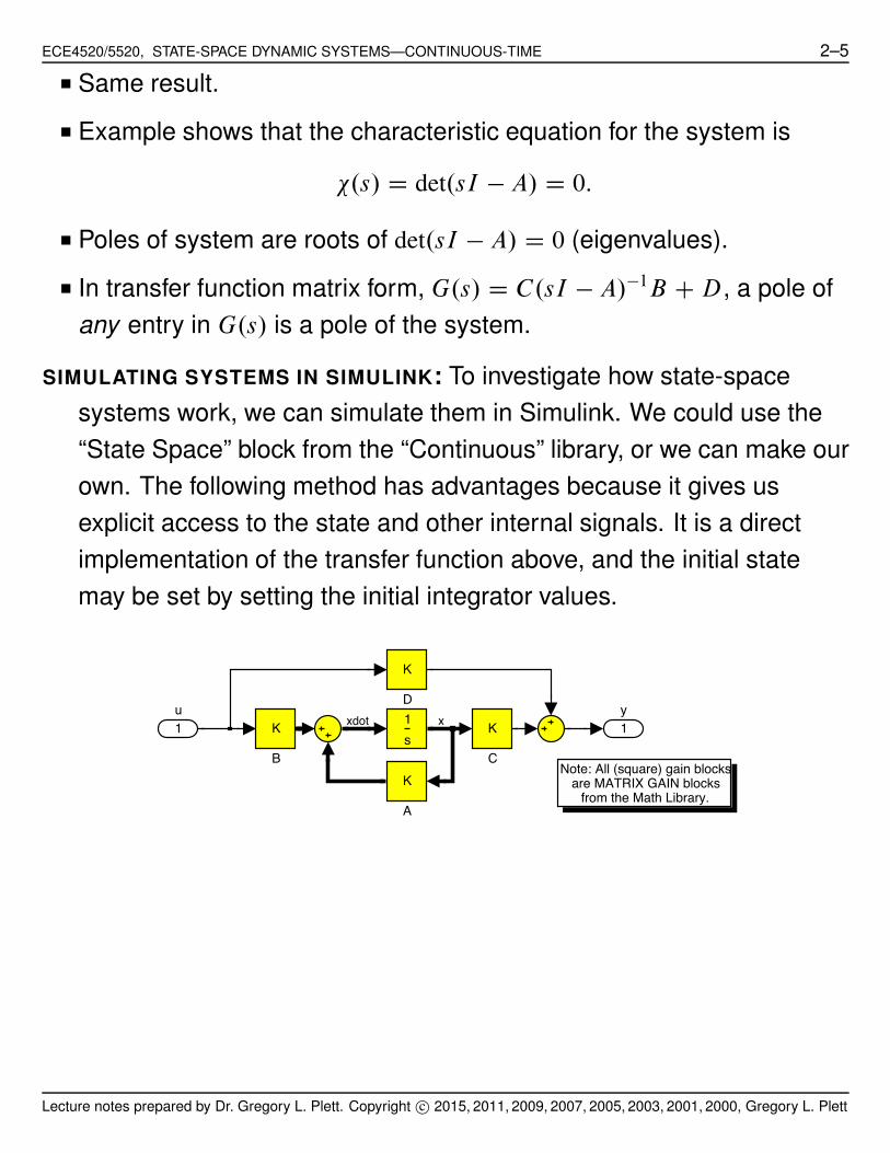
SIMULATING SYSTEMS IN SIMULINK: To investigate how state-space
systems work, we can simulate them in Simulink. We could use the
“State Space” block from the “Continuous” library, or we can make our
own. The following method has advantages because it gives us
explicit access to the state and other internal signals. It is a direct
implementation of the transfer function above, and the initial state
may be set by setting the initial integrator values.
Note: All (square) gain blocks are MATRIX GAIN blocks
from the Math Library.
1y
s1
K
D
K
C
K
BK
A
1u
xdot x
Lecture notes prepared by Dr. Gregory L. Plett. Copyright c" 2015, 2011, 2009, 2007, 2005, 2003, 2001, 2000, Gregory L. Plett
ECE4520/5520, STATE-SPACE DYNAMIC SYSTEMS—CONTINUOUS-TIME 2–6
2.2: Four canonical forms for LTI state-space models
■ We can make state-space forms from EOM, as we have seen.
■ Also from transfer functions: there are four main standardized forms,
plus a couple of other forms we will look at later.
Controller canonical form
■ Three cases:
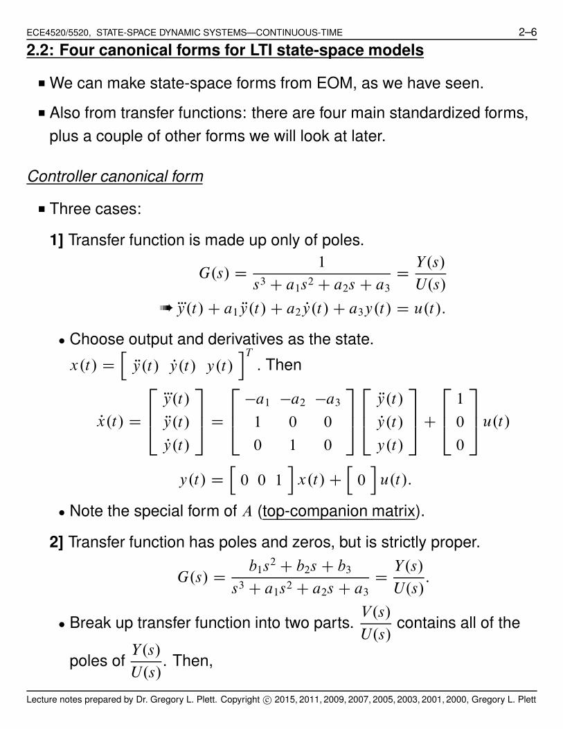
1] Transfer function is made up only of poles.
G.s/ D1
s3 C a1s2 C a2s C a3
DY.s/
U.s/
➠ «y.t/ C a1 Ry.t/ C a2 Py.t/ C a3y.t/ D u.t/:
$ Choose output and derivatives as the state.
x.t/ Dh
Ry.t/ Py.t/ y.t/iT
: Then
Px.t/ D
2
64
«y.t/
Ry.t/
Py.t/
3
75 D
2
64
!a1 !a2 !a3
1 0 0
0 1 0
3
75
2
64
Ry.t/
Py.t/
y.t/
3
75C
2
64
1
0
0
3
75u.t/
y.t/ Dh
0 0 1i
x.t/ Ch
0i
u.t/:
$ Note the special form of A (top-companion matrix).
2] Transfer function has poles and zeros, but is strictly proper.
G.s/ Db1s
2 C b2s C b3
s3 C a1s2 C a2s C a3D
Y.s/
U.s/:
$ Break up transfer function into two parts.V.s/
U.s/contains all of the
poles ofY.s/
U.s/. Then,
Lecture notes prepared by Dr. Gregory L. Plett. Copyright c" 2015, 2011, 2009, 2007, 2005, 2003, 2001, 2000, Gregory L. Plett
ECE4520/5520, STATE-SPACE DYNAMIC SYSTEMS—CONTINUOUS-TIME 2–7
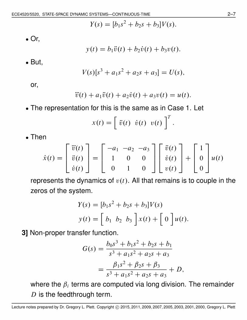
Y.s/ D Œb1s2 C b2s C b3"V.s/:
$ Or,
y.t/ D b1 Rv.t/ C b2 Pv.t/ C b3v.t/:
$ But,
V.s/Œs3 C a1s2 C a2s C a3" D U.s/;
or,
«v.t/ C a1 Rv.t/ C a2 Pv.t/ C a3v.t/ D u.t/:
$ The representation for this is the same as in Case 1. Let
x.t/ Dh
Rv.t/ Pv.t/ v.t/iT
:
$ Then
Px.t/ D
2
64
«v.t/
Rv.t/
Pv.t/
3
75 D
2
64
!a1 !a2 !a3
1 0 0
0 1 0
3
75
2
64
Rv.t/
Pv.t/
v.t/
3
75C
2
64
1
0
0
3
75u.t/
represents the dynamics of v.t/. All that remains is to couple in the
zeros of the system.
Y.s/ D Œb1s2 C b2s C b3"V.s/
y.t/ Dh
b1 b2 b3
i
x.t/ Ch
0i
u.t/:
3] Non-proper transfer function.
G.s/ Db0s
3 C b1s2 C b2s C b1
s3 C a1s2 C a2s C a3
Dˇ1s
2 C ˇ2s C ˇ3
s3 C a1s2 C a2s C a3C D;
where the ˇi terms are computed via long division. The remainder
D is the feedthrough term.
Lecture notes prepared by Dr. Gregory L. Plett. Copyright c" 2015, 2011, 2009, 2007, 2005, 2003, 2001, 2000, Gregory L. Plett
ECE4520/5520, STATE-SPACE DYNAMIC SYSTEMS—CONTINUOUS-TIME 2–8
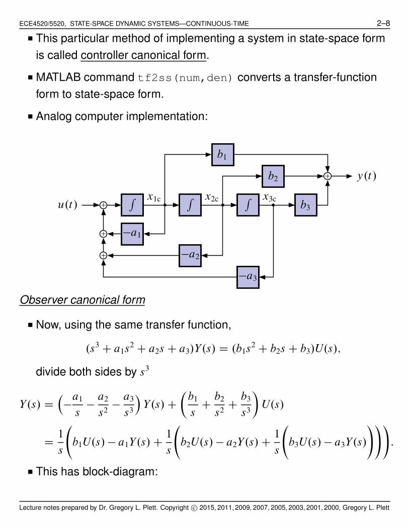
■ This particular method of implementing a system in state-space form
is called controller canonical form.
■ MATLAB command tf2ss(num,den) converts a transfer-function
form to state-space form.
■ Analog computer implementation:
y.t/
u.t/x1c x2c x3cR R R
b1
b2
b3
!a1
!a2
!a3
Observer canonical form
■ Now, using the same transfer function,
.s3 C a1s2 C a2s C a3/Y.s/ D .b1s
2 C b2s C b3/U.s/;
divide both sides by s3
Y.s/ D!
!a1
s!
a2
s2!
a3
s3
"
Y.s/ C#
b1
sC
b2
s2C
b3
s3
$
U.s/
D1
s
b1U.s/ ! a1Y.s/ C1
s
b2U.s/ ! a2Y.s/ C1
s
b3U.s/ ! a3Y.s/
!!!
:
■ This has block-diagram:
Lecture notes prepared by Dr. Gregory L. Plett. Copyright c" 2015, 2011, 2009, 2007, 2005, 2003, 2001, 2000, Gregory L. Plett

ECE4520/5520, STATE-SPACE DYNAMIC SYSTEMS—CONTINUOUS-TIME 2–9
y.t/
u.t/
x1ox2ox3o R RR
b1b2b3
!a1!a2!a3
■ This is called observer canonical form:
Px.t/ D
2
64
!a1 1 0
!a2 0 1
!a3 0 0
3
75x.t/ C
2
64
b1
b2
b3
3
75u.t/
y.t/ Dh
1 0 0i
x.t/:
■ A is a left-companion matrix.
Controllability canonical form
■ Third, consider the block diagram:
y.t/
u.t/
x1co x2cox3coRR R
ˇ1
ˇ2
ˇ3
!a1!a2!a3
Lecture notes prepared by Dr. Gregory L. Plett. Copyright c" 2015, 2011, 2009, 2007, 2005, 2003, 2001, 2000, Gregory L. Plett
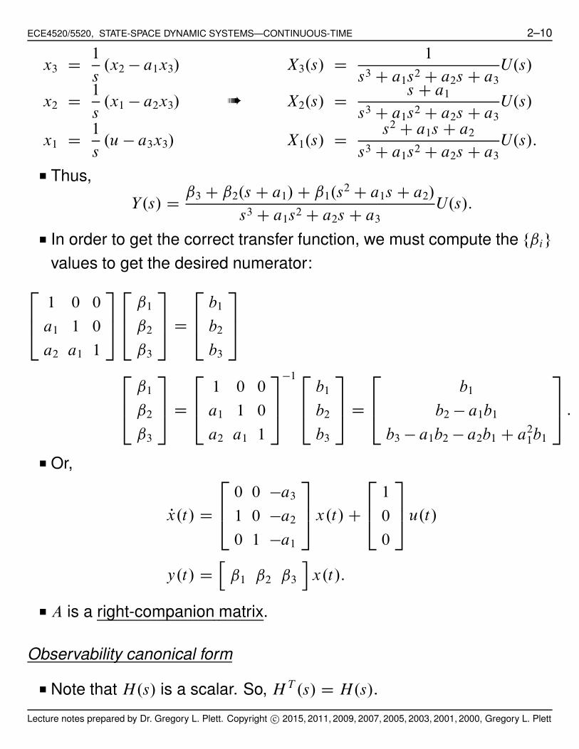
ECE4520/5520, STATE-SPACE DYNAMIC SYSTEMS—CONTINUOUS-TIME 2–10
x3 D1
s.x2 ! a1x3/ X3.s/ D
1
s3 C a1s2 C a2s C a3
U.s/
x2 D1
s.x1 ! a2x3/ ➠ X2.s/ D
s C a1
s3 C a1s2 C a2s C a3
U.s/
x1 D1
s.u ! a3x3/ X1.s/ D
s2 C a1s C a2
s3 C a1s2 C a2s C a3
U.s/:
■ Thus,
Y.s/ Dˇ3 C ˇ2.s C a1/ C ˇ1.s
2 C a1s C a2/
s3 C a1s2 C a2s C a3
U.s/:
■ In order to get the correct transfer function, we must compute the fˇigvalues to get the desired numerator:
2
64
1 0 0
a1 1 0
a2 a1 1
3
75
2
64
ˇ1
ˇ2
ˇ3
3
75 D
2
64
b1
b2
b3
3
75
2
64
ˇ1
ˇ2
ˇ3
3
75 D
2
64
1 0 0
a1 1 0
a2 a1 1
3
75
!12
64
b1
b2
b3
3
75 D
2
64
b1
b2 ! a1b1
b3 ! a1b2 ! a2b1 C a21b1
3
75 :
■ Or,
Px.t/ D
2
64
0 0 !a3
1 0 !a2
0 1 !a1
3
75x.t/ C
2
64
1
0
0
3
75u.t/
y.t/ Dh
ˇ1 ˇ2 ˇ3
i
x.t/:
■ A is a right-companion matrix.
Observability canonical form
■ Note that H.s/ is a scalar. So, H T .s/ D H.s/.
Lecture notes prepared by Dr. Gregory L. Plett. Copyright c" 2015, 2011, 2009, 2007, 2005, 2003, 2001, 2000, Gregory L. Plett

ECE4520/5520, STATE-SPACE DYNAMIC SYSTEMS—CONTINUOUS-TIME 2–11
H.s/ D C.sI ! A/!1B C D
D BT .sI ! A/!T C T C DT
D BT .sI ! AT /!1C T C DT :
■ So, C $ BT , A $ AT , B $ C T and D $ DT are dual forms.
■ We have already seen this(!). Controller and observer are dual forms.
Likewise, we can come up with
Px.t/ D
2
64
0 1 0
0 0 1
!a3 !a2 !a1
3
75 x.t/ C
2
64
ˇ1
ˇ2
ˇ3
3
75u.t/
y.t/ Dh
1 0 0i
x.t/
as a dual form with the controllability form.
y.t/
u.t/
x1obx2obx3ob RRR
ˇ1ˇ2ˇ3
!a1
!a2
!a3
■ A is a bottom-companion matrix.
■ We will see that we have a lot of freedom when making our
state-space models (i.e., in choosing the components of x.t/).
Lecture notes prepared by Dr. Gregory L. Plett. Copyright c" 2015, 2011, 2009, 2007, 2005, 2003, 2001, 2000, Gregory L. Plett

ECE4520/5520, STATE-SPACE DYNAMIC SYSTEMS—CONTINUOUS-TIME 2–12
2.3: One more canonical form, transformations
Modal (diagonal) form
■ Yet another “canonical” form. Very useful. . .
■ Assume G.s/ DN.s/
D.s/; D.s/ has distinct roots pi (real).
G.s/ DN.s/
.s ! p1/.s ! p2/ % % % .s ! pn/
Dr1
s ! p1
Cr2
s ! p2
C % % % Crn
s ! pn
:
■ Now, let
X1.s/
U.s/D
r1
s ! p1
➠ Px1.t/ D p1x1.t/ C r1u.t/
:::
Xn.s/
U.s/D
rn
s ! pn
➠ Pxn.t/ D pnxn.t/ C rnu.t/:
■ Or,
Px.t/ D Ax.t/ C Bu.t/
y.t/ D Cx.t/ C Du.t/
A D
2
66664
p1 0
p2
: : :
0 pn
3
77775
; B D
2
66664
r1
r2:::
rn
3
77775
C Dh
1 1 % % % 1i
; D Dh
0i
:
■ Easily extends to handle complex poles $i D %i C j!i .
Lecture notes prepared by Dr. Gregory L. Plett. Copyright c" 2015, 2011, 2009, 2007, 2005, 2003, 2001, 2000, Gregory L. Plett

ECE4520/5520, STATE-SPACE DYNAMIC SYSTEMS—CONTINUOUS-TIME 2–13
$ If A and B may have complex elements, no change is necessary.
$ Otherwise, use “real modal form” which is made via partial-fraction
expansion where complex pole-pairs are represented as
Gi.s/ D˛is C ˇi
.s ! %i /2 C !2i
:
$ The real-modal form has an A matrix which is block diagonal, and
of the form
A D diag
ƒr;
"
%rC1 !rC1
!!rC1 %rC1
#
; : : : ;
"
%n !n
!!n %n
#!
where ƒr is a diagonal matrix containing the real poles, and
$i D %i C j!i; i D r C 1; : : : ; n
are the complex poles.
$ The B matrix has corresponding entries:"
bi;1
bi;2
#
D
"
1 1
!!i ! %i !i ! %i
#!1 "
˛i
ˇi
#
:
■ Modal form is convenient for keeping track of system poles: : : they
are right on the diagonal!
■ Good representation to use: : : numerical robustness.
■ All canonical forms related by linear algebra—change of basis.
■ Diagonal is very useful, but we cannot always put a system in
diagonal form. (What was our assumption above?)
■ We will see one more canonical (Jordan) form in a little while that is
very similar to diagonal. All systems can be put in Jordan form.
Lecture notes prepared by Dr. Gregory L. Plett. Copyright c" 2015, 2011, 2009, 2007, 2005, 2003, 2001, 2000, Gregory L. Plett
ECE4520/5520, STATE-SPACE DYNAMIC SYSTEMS—CONTINUOUS-TIME 2–14
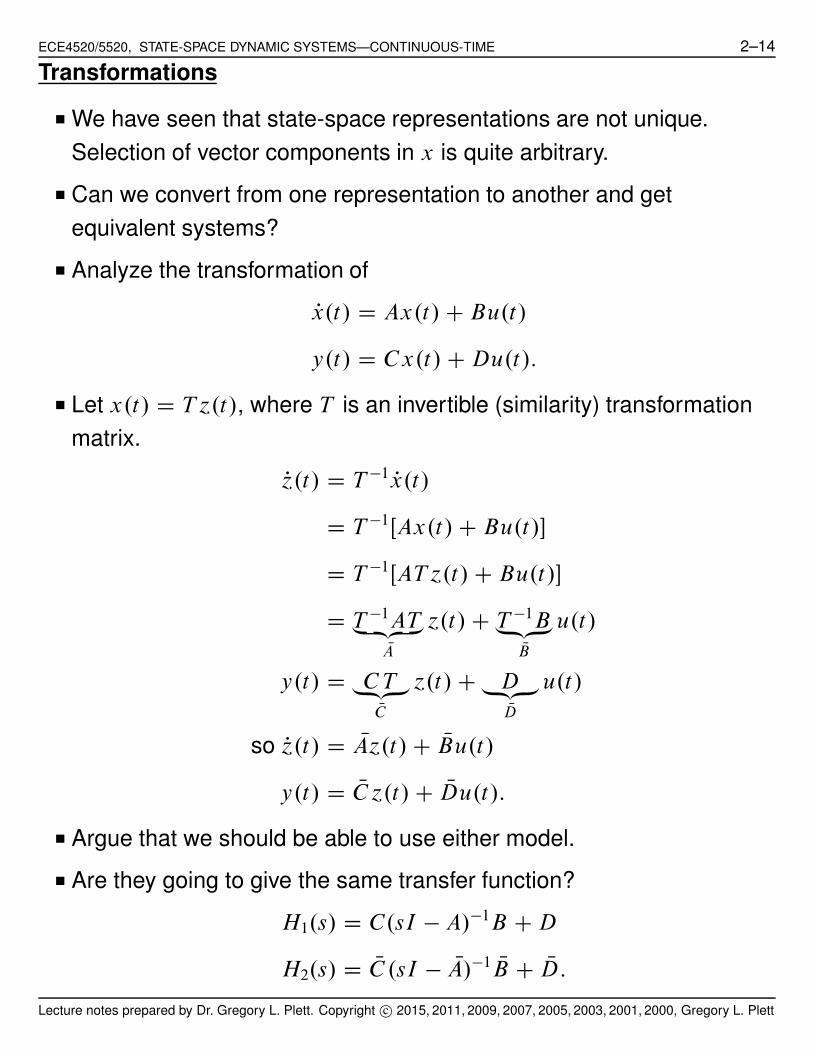
Transformations
■ We have seen that state-space representations are not unique.
Selection of vector components in x is quite arbitrary.
■ Can we convert from one representation to another and get
equivalent systems?
■ Analyze the transformation of
Px.t/ D Ax.t/ C Bu.t/
y.t/ D Cx.t/ C Du.t/:
■ Let x.t/ D T ´.t/, where T is an invertible (similarity) transformation
matrix.
P.t/ D T !1 Px.t/
D T !1ŒAx.t/ C Bu.t/"
D T !1ŒAT ´.t/ C Bu.t/"
D T !1AT„ ƒ‚ …
NA
´.t/ C T !1B„ƒ‚…
NB
u.t/
y.t/ D C T„ƒ‚…
NC
´.t/ C D„ƒ‚…
ND
u.t/
so P.t/ D NA´.t/ C NBu.t/
y.t/ D NC ´.t/ C NDu.t/:
■ Argue that we should be able to use either model.
■ Are they going to give the same transfer function?
H1.s/ D C.sI ! A/!1B C D
H2.s/ D NC .sI ! NA/!1 NB C ND:
Lecture notes prepared by Dr. Gregory L. Plett. Copyright c" 2015, 2011, 2009, 2007, 2005, 2003, 2001, 2000, Gregory L. Plett
ECE4520/5520, STATE-SPACE DYNAMIC SYSTEMS—CONTINUOUS-TIME 2–15
■ Need H1.s/ D H2.s/.
H1.s/ D C.sI ! A/!1B C D
D C T T !1.sI ! A/!1T T !1B C D
D .C T /ŒT !1.sI ! A/T "!1.T !1B/ C D
D NC .sI ! NA/!1 NB C ND D H2.s/:
Transfer function not changed by similarity transform.
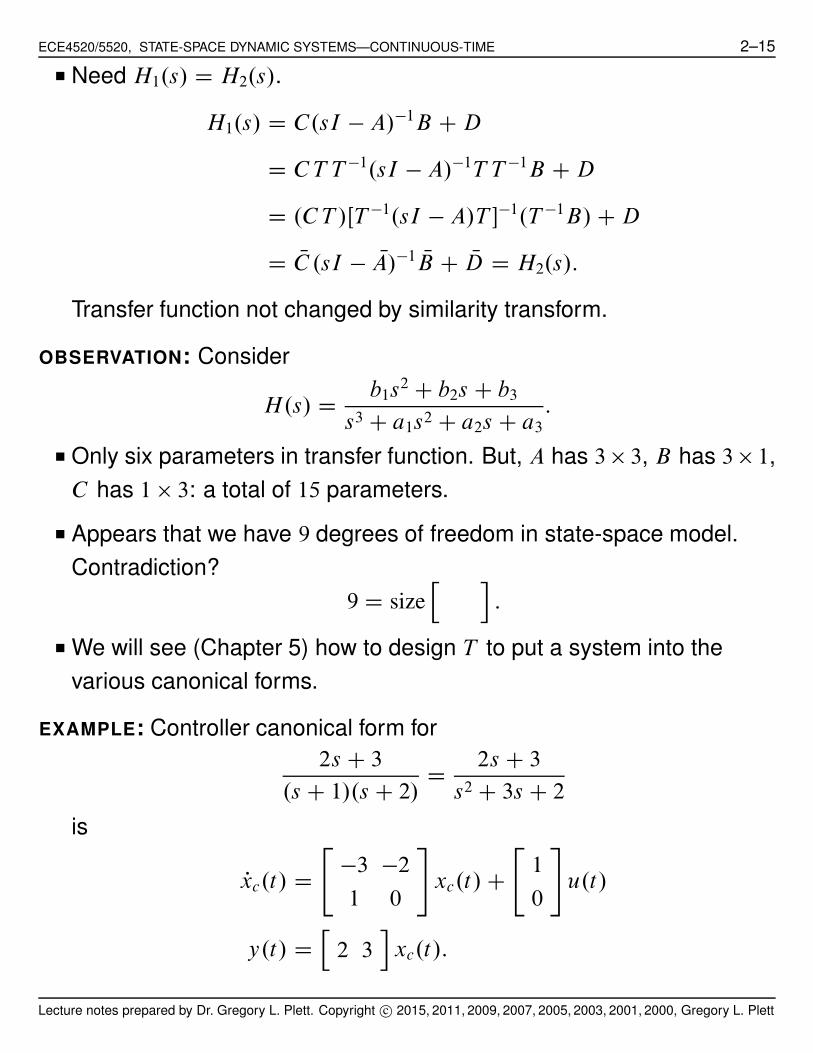
OBSERVATION: Consider
H.s/ Db1s
2 C b2s C b3
s3 C a1s2 C a2s C a3:
■ Only six parameters in transfer function. But, A has 3 & 3, B has 3 & 1,
C has 1 & 3: a total of 15 parameters.
■ Appears that we have 9 degrees of freedom in state-space model.
Contradiction?
9 D sizeh i
:
■ We will see (Chapter 5) how to design T to put a system into the
various canonical forms.
EXAMPLE: Controller canonical form for
2s C 3
.s C 1/.s C 2/D
2s C 3
s2 C 3s C 2
is
Pxc.t/ D
"
!3 !2
1 0
#
xc.t/ C
"
1
0
#
u.t/
y.t/ Dh
2 3i
xc.t/:
Lecture notes prepared by Dr. Gregory L. Plett. Copyright c" 2015, 2011, 2009, 2007, 2005, 2003, 2001, 2000, Gregory L. Plett

ECE4520/5520, STATE-SPACE DYNAMIC SYSTEMS—CONTINUOUS-TIME 2–16
■ Suppose we have the transformation matrix (note: det.T / D 1 so T is
invertible).
T D
"
2 !1
!1 1
#
:
■ Let xc D T Nx, where Nx is a new state. Then,
PNx.t/ D .T !1AT / Nx.t/ C .T !1B/u.t/
y.t/ D .C T / Nx.t/:
■ Plugging in A, B, C and T :
PNx.t/ D
"
!2 0
0 !1
#
Nx.t/ C
"
1
1
#
u.t/
y.t/ Dh
1 1i
Nx.t/;
which gives the diagonal realization of the transfer function!
■ We’ll often change coordinates in a system, for example to solve a
particular problem more easily.
EXAMPLE: Consider the system in the above example, implemented in
the four main canonical forms. Let the initial state for each form be
x.0/ D Œ1 1"T . Simulate response of each system.
■ The systems have the same
transfer function, but different
responses to initial states since
the states have different
interpretations.
0 1 2 3 4 5 6−1
0
1
2
3
4
5
Time
Am
plit
ude
Initial responses for same initial state
Lecture notes prepared by Dr. Gregory L. Plett. Copyright c" 2015, 2011, 2009, 2007, 2005, 2003, 2001, 2000, Gregory L. Plett

ECE4520/5520, STATE-SPACE DYNAMIC SYSTEMS—CONTINUOUS-TIME 2–17
2.4: Time (dynamic) response
■ Develop more insight into the system response by looking at
time-domain solution for x.t/.
■ Scalar case first, then many states and MIMO.
Homogeneous part (scalar)
■ Px.t/ D ax.t/; x.0/.
■ Take Laplace. X.s/ D .s ! a/!1x.0/.
■ Inverse Laplace. x.t/ D eatx.0/.
Homogeneous part (full solution)
■ Px.t/ D Ax.t/; x.0/.
■ Take Laplace. X.s/ D .sI ! A/!1x.0/.
■ x.t/ D L!1Œ.sI ! A/!1"x.0/.
■ But,
.sI ! A/!1 DI
sC
A
s2C
A2
s3C % % %
so,
L!1Œ.sI ! A/!1" D I C At CA2t2
2ŠC
A3t3
3ŠC % % %
4D eAt matrix exponential
x.t/ D eAtx.0/:
■ eAt is called the transition matrix or state-transition matrix.
■ Matrix exponential expm.m
Lecture notes prepared by Dr. Gregory L. Plett. Copyright c" 2015, 2011, 2009, 2007, 2005, 2003, 2001, 2000, Gregory L. Plett

ECE4520/5520, STATE-SPACE DYNAMIC SYSTEMS—CONTINUOUS-TIME 2–18
■ e.ACB/t D eAteBt iff AB D BA: (i.e., not in general).
■ Will say more about eAt when we discuss the structure of A.
■ Computation of eAt D L!1Œ.sI ! A/!1" straightforward for 2 & 2.
EXAMPLE:
Px D Ax; A D
"
0 1
!2 !3
#
.sI ! A/!1 D
"
s !1
2 s C 3
#!1
D
"
s C 3 1
!2 s
#
1
.s C 2/.s C 1/
D
2
664
2
s C 1!
1
s C 2
1
s C 1!
1
s C 2!2
s C 1C
2
s C 2
!1
s C 1C
2
s C 2
3
775
eAt D
"
2e!t ! e!2t e!t ! e!2t
!2e!t C 2e!2t !e!t C 2e!2t
#
1.t/
■ This is the best way to find eAt if A 2 & 2.
Forced solution (scalar)
Px.t/ D ax.t/ C bu.t/; x.0/
x.t/ D eatx.0/ CZ t
0
ea.t!!/bu.!/ d!„ ƒ‚ …
convolution
:
■ Where did this come from?
1. Px.t/ ! ax.t/ D bu.t/
2. e!at ΠPx.t/ ! ax.t/" Dd
dtŒe!atx.t/" D e!atbu.t/:
Lecture notes prepared by Dr. Gregory L. Plett. Copyright c" 2015, 2011, 2009, 2007, 2005, 2003, 2001, 2000, Gregory L. Plett
ECE4520/5520, STATE-SPACE DYNAMIC SYSTEMS—CONTINUOUS-TIME 2–19
3.
Z t
0
d
d!Œe!a!x.!/" d! D e!atx.t/ ! x.0/ D
Z t
0
e!a!bu.!/ d!:
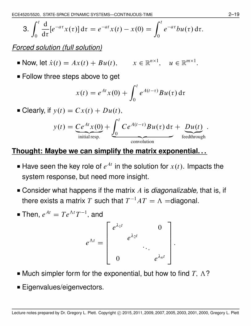
Forced solution (full solution)
■ Now, let Px.t/ D Ax.t/ C Bu.t/; x 2 Rn&1; u 2 R
m&1:
■ Follow three steps above to get
x.t/ D eAtx.0/ CZ t
0
eA.t!!/Bu.!/ d!
■ Clearly, if y.t/ D Cx.t/ C Du.t/;
y.t/ D CeAtx.0/„ ƒ‚ …
initial resp:
CZ t
0
CeA.t!!/Bu.!/ d!„ ƒ‚ …
convolution
C Du.t/„ƒ‚…
feedthrough
:
Thought: Maybe we can simplify the matrix exponential. . .
■ Have seen the key role of eAt in the solution for x.t/. Impacts the
system response, but need more insight.
■ Consider what happens if the matrix A is diagonalizable, that is, if
there exists a matrix T such that T !1AT D ƒ Ddiagonal.
■ Then, eAt D TeƒtT !1; and
eƒt D
2
66664
e$1t 0
e$2t
: : :
0 e$nt
3
77775
:
■ Much simpler form for the exponential, but how to find T; ƒ?
■ Eigenvalues/eigenvectors.
Lecture notes prepared by Dr. Gregory L. Plett. Copyright c" 2015, 2011, 2009, 2007, 2005, 2003, 2001, 2000, Gregory L. Plett
ECE4520/5520, STATE-SPACE DYNAMIC SYSTEMS—CONTINUOUS-TIME 2–20
2.5: Diagonalizing the A matrix
■ “Eigen” is a German word meaning “self” or “characteristic”.
■ The eigenvectors and eigenvalues of A characterize its behavior.
■ An eigenvector is a vector satisfying
Av D $v;
where $ is a (possibly complex) constant, and v ¤ 0.
■ Multiplying by A does nothing to the vector except change its length!
■ This is a very unusual vector. There are usually only n of them if A
has size n & n.
$ Note that if v is an eigenvector, kv is also an eigenvector—so
eigenvectors are often normalized to have unit length: kvk2 D 1.
■ The constant $ is an eigenvalue. Specifically, it is the eigenvalue
associated with eigenvector v.
■ Since there are (usually) n eigenvectors with n corresponding
eigenvalues, we label the eigenvectors and eigenvalues vi and $i
where 1 ' i ' n.
■ To find eigenvalues, consider that .$I ! A/v D 0.
■ Since v ¤ 0, $I ! A must drop rank for some value of $ associated
with v. A matrix which is not full rank has zero determinant. So, we
can solve for the eigenvalues by solving
det.$I ! A/ D 0:
■ We have seen already that this is how we solve for the poles of a
state-space system, so the eigenvalues of the A matrix are the poles
of the dynamic system.
Lecture notes prepared by Dr. Gregory L. Plett. Copyright c" 2015, 2011, 2009, 2007, 2005, 2003, 2001, 2000, Gregory L. Plett

ECE4520/5520, STATE-SPACE DYNAMIC SYSTEMS—CONTINUOUS-TIME 2–21
■ There are very efficient and numerically robust methods of finding
eigenvectors/values. These methods do not use the determinant rule,
above. The determinant rule is useful for mathematical analysis.
■ In MATLAB, [V,Lambda]=eig(A);
Example: Finding eigenvalues/eigenvectors of 2 & 2 matrix
■ Let
A D
"
3 3
!5 !5
#
:
■ To find eigenvalues, we solve:
det.$I ! A/ D 0
det
"
$ 0
0 $
#
!
"
3 3
!5 !5
#!
D 0
det
"
$ ! 3 !3
5 $ C 5
#!
D 0
.$ ! 3/.$ C 5/ C 15 D 0
$2 C 2$ D 0:
■ We see that there are eigenvalues at $1 D 0 and $2 D !2.
■ To find eigenvector corresponding to $1 D 0, we solve
Av1 D $1v1"
3 3
!5 !5
#"
v1a
v1b
#
D 0
"
v1a
v1b
#
:
■ This gives us the equation that v1a D !v1b. We can arbitrarily choose
one component, so let v1a D 1 giving v1 Dh
1 !1iT
.
Lecture notes prepared by Dr. Gregory L. Plett. Copyright c" 2015, 2011, 2009, 2007, 2005, 2003, 2001, 2000, Gregory L. Plett

ECE4520/5520, STATE-SPACE DYNAMIC SYSTEMS—CONTINUOUS-TIME 2–22
■ We should further normalize this to have unit length by dividing byp
.1/2 C .!1/2. This gives
vnormalized1 D
"
1=p
2
!1=p
2
#
:
■ We find the second eigenvector similarly:"
3 3
!5 !5
#"
v2a
v2b
#
D !2
"
v2a
v2b
#
:
■ Again, arbitrarily choose v2a D 1. Then, we find that v2b D !5=3.
■ We can normalize by dividing byp
.1/2 C .!5=3/2. We get the answer
vnormalized2 D
"
0:5145
0:8575
#
:
The diagonal form
■ Assume that eigenvectors v1; v2; : : : vn are linearly independent.
Stack together in a matrix equation:
Avi D $ivi i D 1; 2; : : : ; n
Ah
v1 v2 : : : vn
i
„ ƒ‚ …
T
Dh
v1 v2 : : : vn
i
2
64
$1 0: : :
0 $n
3
75
„ ƒ‚ …
ƒ
■ AT D Tƒ ➠ T !1AT D V !1AV D ƒ.
■ We have found the transformation matrix T that diagonalizes A!
■ However, not all matrices are diagonalizable. For example,
A D
"
0 1
0 0
#
det.$I ! A/ D $2:
Lecture notes prepared by Dr. Gregory L. Plett. Copyright c" 2015, 2011, 2009, 2007, 2005, 2003, 2001, 2000, Gregory L. Plett

ECE4520/5520, STATE-SPACE DYNAMIC SYSTEMS—CONTINUOUS-TIME 2–23
■ One eigenvalue $ D 0. Solve for the eigenvectors"
0 1
0 0
#"
va
vb
#
D 0 ➠ all vectors of the form
"
va
0
#
¤ 0:
Dynamic interpretation using diagonal form
■ Diagonal form makes it easier to understand what is happening in a
state-space dynamic system.
$ Assume A is diagonalizable by T D V .
$ Define new coordinates by x.t/ D T Qx.t/ so
PQx.t/ D T !1Ax.t/ D T !1AT Qx.t/ D ƒ Qx.t/:
$ In new coordinate system, system is diagonal (decoupled).
■ Trajectories consist of n independent modes; that is,
Qxi.t/ D e$i t Qxi.0/
hence the name, modal form.
■ To understand in original coordinate system, write T !1AT D ƒ as
T !1A D ƒT !1 with
T !1 D
2
66664
wT1
wT2:::
wTn
3
77775
; i:e:; rows of T !1:
wTi A D $iw
Ti ; so wi is a left eigenvector of A and note that
wTi vj D ıi;j .
■ How does this help?
eAt D TeƒtT !1
Lecture notes prepared by Dr. Gregory L. Plett. Copyright c" 2015, 2011, 2009, 2007, 2005, 2003, 2001, 2000, Gregory L. Plett
ECE4520/5520, STATE-SPACE DYNAMIC SYSTEMS—CONTINUOUS-TIME 2–24
Dh
v1 v2 : : : vn
i
2
66664
e$1t 0
e$2t
: : :
0 e$nt
3
77775
2
66664
wT1
wT2:::
wnT
3
77775
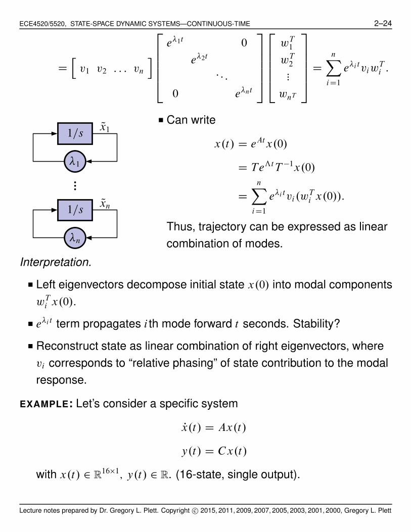
DnX
iD1
e$i t viwTi :
1=s
1=s
$1
$n
Qx1
Qxn
■ Can write
x.t/ D eAtx.0/
D TeƒtT !1x.0/
DnX
iD1
e$i tvi .wTi x.0//:
Thus, trajectory can be expressed as linear
combination of modes.
Interpretation.
■ Left eigenvectors decompose initial state x.0/ into modal components
wTi x.0/:
■ e$i t term propagates i th mode forward t seconds. Stability?
■ Reconstruct state as linear combination of right eigenvectors, where
vi corresponds to “relative phasing” of state contribution to the modal
response.
EXAMPLE: Let’s consider a specific system
Px.t/ D Ax.t/
y.t/ D Cx.t/
with x.t/ 2 R16&1; y.t/ 2 R. (16-state, single output).
Lecture notes prepared by Dr. Gregory L. Plett. Copyright c" 2015, 2011, 2009, 2007, 2005, 2003, 2001, 2000, Gregory L. Plett

ECE4520/5520, STATE-SPACE DYNAMIC SYSTEMS—CONTINUOUS-TIME 2–25
■ A lightly damped system.
■ Typical output to initial
conditions shown.
■ Output waveform is very
complicated. Looks almost
random.0 50 100 150 200 250 300
−2
−1.5
−1
−0.5
0
0.5
1
1.5
2
Impulse Response
Am
plit
ude
Time (sec.)
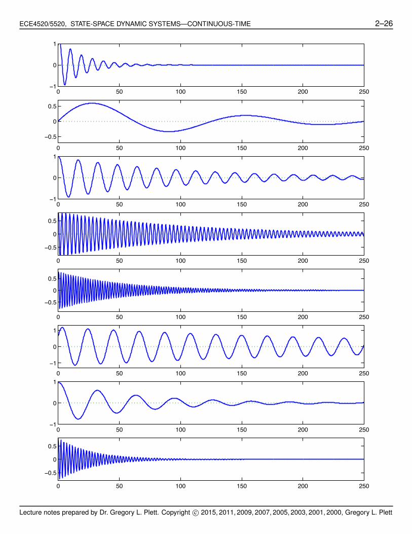
■ However, such a solution can be decomposed into much simpler
modal components (see next page).
BOTTOM LINE: While responses of state-space systems can appear very
complicated, they are fundamentally simply summations of very
simple responses. Poles (eigenvalues of) A determine character of
the response.
Lecture notes prepared by Dr. Gregory L. Plett. Copyright c" 2015, 2011, 2009, 2007, 2005, 2003, 2001, 2000, Gregory L. Plett
ECE4520/5520, STATE-SPACE DYNAMIC SYSTEMS—CONTINUOUS-TIME 2–26
0 50 100 150 200 250−1
0
1
0 50 100 150 200 250
−0.5
0
0.5
0 50 100 150 200 250−1
0
1
0 50 100 150 200 250
−0.5
0
0.5
0 50 100 150 200 250
−0.5
0
0.5
0 50 100 150 200 250−1
0
1
0 50 100 150 200 250−1
0
1
0 50 100 150 200 250
−0.5
0
0.5
Lecture notes prepared by Dr. Gregory L. Plett. Copyright c" 2015, 2011, 2009, 2007, 2005, 2003, 2001, 2000, Gregory L. Plett
ECE4520/5520, STATE-SPACE DYNAMIC SYSTEMS—CONTINUOUS-TIME 2–27
2.6: The Jordan canonical form; MIMO canonical forms
■ What if A cannot be diagonalized?
■ Any matrix A 2 Rn&n can be put in Jordan canonical form by a
similarity transformation.
■ That is, we can find a transformation matrix T such that T !1AT D J ,
where J is a matrix in Jordan form.
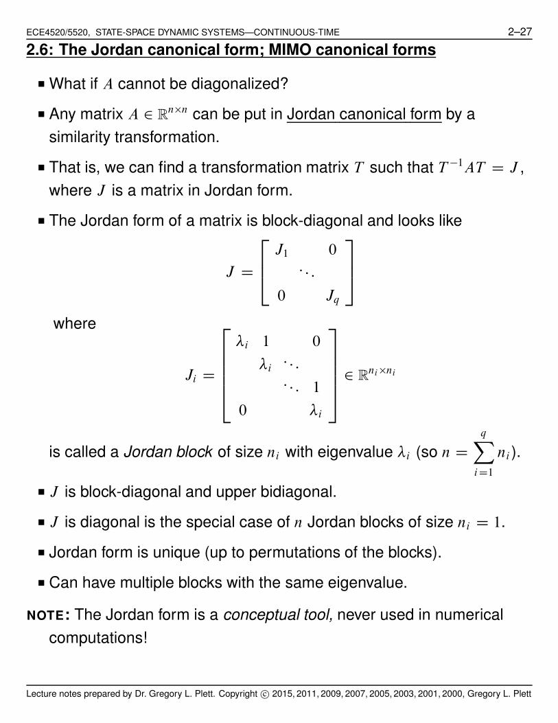
■ The Jordan form of a matrix is block-diagonal and looks like
J D
2
64
J1 0: : :
0 Jq
3
75
where
Ji D
2
66664
$i 1 0
$i: : :: : : 1
0 $i
3
77775
2 Rni&ni
is called a Jordan block of size ni with eigenvalue $i (so n DqX
iD1
ni).
■ J is block-diagonal and upper bidiagonal.
■ J is diagonal is the special case of n Jordan blocks of size ni D 1.
■ Jordan form is unique (up to permutations of the blocks).
■ Can have multiple blocks with the same eigenvalue.
NOTE: The Jordan form is a conceptual tool, never used in numerical
computations!
Lecture notes prepared by Dr. Gregory L. Plett. Copyright c" 2015, 2011, 2009, 2007, 2005, 2003, 2001, 2000, Gregory L. Plett

ECE4520/5520, STATE-SPACE DYNAMIC SYSTEMS—CONTINUOUS-TIME 2–28
■ #.$/ D det.$I ! A/ D det.$I ! J / D .$ ! $1/n1 % % % .$ ! $q/nq D 0 hence
distinct eigenvalues ➠ ni D 1 ➠ A diagonalizable.
■ dimN .$iI ! A/ D dimN .$iI ! J / is the number of Jordan blocks with
eigenvalue $i .
■ The sizes of each Jordan block may also be computed, but this is
complicated. i.e., leave it to MATLAB! ➠ jordan(A)
EXAMPLE: Consider
A D
2
6666666664
3 !1 1 1 0 0
1 1 !1 !1 0 0
0 0 2 0 1 1
0 0 0 2 !1 !1
0 0 0 0 1 1
0 0 0 0 1 1
3
7777777775
:
■ From MATLAB, we find that A has eigenvalue 2 with multiplicity 5 and
eigenvalue 0 with multiplicity 1:
det.$I ! A/ D .$ ! 2/5$:
■ rank.2I ! A/ D 4, so dim.N .2I ! A// D 6 ! 4 D 2 so there are two
Jordan blocks with eigenvalue 2.
■ We can check this in MATLAB: jordan(A)
J D
2
6666666664
0 0 0 0 0 0
0 2 1 0 0 0
0 0 2 1 0 0
0 0 0 2 0 0
0 0 0 0 2 1
0 0 0 0 0 2
3
7777777775
Lecture notes prepared by Dr. Gregory L. Plett. Copyright c" 2015, 2011, 2009, 2007, 2005, 2003, 2001, 2000, Gregory L. Plett

ECE4520/5520, STATE-SPACE DYNAMIC SYSTEMS—CONTINUOUS-TIME 2–29
■ Note that without further information (computation) the following form
might also be the Jordan form for A (but it isn’t)
J D
2
6666666664
0 0 0 0 0 0
0 2 0 0 0 0
0 0 2 1 0 0
0 0 0 2 1 0
0 0 0 0 2 1
0 0 0 0 0 2
3
7777777775
■ System written in Jordan form is decomposed into independent
Jordan block systems PQxi.t/ D Ji Qxi.t/
y.t/u.t/1
s ! $
1
s ! $
1
s ! $
c1
c2
cn
■ Jordan blocks sometimes called Jordan chains (diagram shows why).
■ What does this mean in the time domain?
.sI ! J$/!1 D
2
66664
s ! $ !1 0
s ! $ : : :: : : !1
0 s ! $
3
77775
!1
D
2
66664
.s ! $/!1 .s ! $/!2 % % % .s ! $/!k
.s ! $/!1 % % % .s ! $/!kC1
: : : :::
0 .s ! $/!1
3
77775
Lecture notes prepared by Dr. Gregory L. Plett. Copyright c" 2015, 2011, 2009, 2007, 2005, 2003, 2001, 2000, Gregory L. Plett
ECE4520/5520, STATE-SPACE DYNAMIC SYSTEMS—CONTINUOUS-TIME 2–30
D .s ! $/!1I C .s ! $/!2F1 C % % % C .s ! $/!kFk
where Fk is the matrix with ones on the kth upper diagonal.
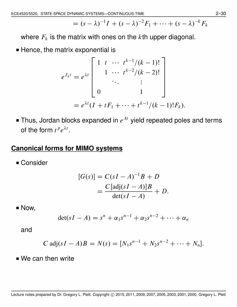
■ Hence, the matrix exponential is
eJ$t D e$t
2
66664
1 t % % % t k!1=.k ! 1/Š
1 % % % t k!2=.k ! 2/Š: : : :::
0 1
3
77775
D e$t .I C tF1 C % % % C t k!1=.k ! 1/ŠFk/:
■ Thus, Jordan blocks expanded in eAt yield repeated poles and terms
of the form tpe$t .
Canonical forms for MIMO systems
■ Consider
ŒG.s/" D C.sI ! A/!1B C D
DC Œadj.sI ! A/"B
det.sI ! A/C D:
■ Now,
det.sI ! A/ D sn C ˛1sn!1 C ˛2s
n!2 C % % % C ˛n
and
C adj.sI ! A/B D N.s/ D ŒN1sn!1 C N2s
n!2 C % % % C Nn":
■ We can then write
Lecture notes prepared by Dr. Gregory L. Plett. Copyright c" 2015, 2011, 2009, 2007, 2005, 2003, 2001, 2000, Gregory L. Plett
ECE4520/5520, STATE-SPACE DYNAMIC SYSTEMS—CONTINUOUS-TIME 2–31
Px.t/ D
2
6666664
!˛1I !˛2I % % % !˛n!1I !˛nI
I 0 0 0
0 I 0 0::: ::: ::: :::
0 0 % % % I 0
3
7777775
x.t/ C
2
6666664
I
0
0:::
0
3
7777775
u.t/
y.t/ Dh
N1 N2 % % % Nn!1 Nn
i
x.t/ C G.1/u.t/;
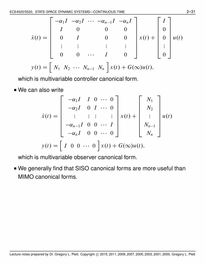
which is multivariable controller canonical form.
■ We can also write
Px.t/ D
2
6666664
!˛1I I 0 % % % 0
!˛2I 0 I % % % 0::: ::: ::: :::
!˛n!1I 0 0 % % % I
!˛nI 0 0 % % % 0
3
7777775
x.t/ C
2
6666664
N1
N2:::
Nn!1
Nn
3
7777775
u.t/
y.t/ Dh
I 0 0 % % % 0i
x.t/ C G.1/u.t/;
which is multivariable observer canonical form.
■ We generally find that SISO canonical forms are more useful than
MIMO canonical forms.
Lecture notes prepared by Dr. Gregory L. Plett. Copyright c" 2015, 2011, 2009, 2007, 2005, 2003, 2001, 2000, Gregory L. Plett
ECE4520/5520, STATE-SPACE DYNAMIC SYSTEMS—CONTINUOUS-TIME 2–32
2.7: Zeros of a state-space system
■ Have seen eigenvalues of A, or poles of the entries of G.s/ are the
poles. Zeros of transfer function?
■ What is a zero? Two types of zero in a MIMO system: Blocking zeros
and transmission zeros.
■ Consider a system with input U.s/ DK
s ! $, K ¤ 0 a constant vector.
■ If $ is a blocking zero, e$t will not appear at the output for any K, x.0/.
(Not considered a very useful definition for MIMO zero).
■ If $ is a transmission zero, e$t will not appear at the output for some
specific K, x.0/.
fblocking zerosg ( ftransmission zerosg:
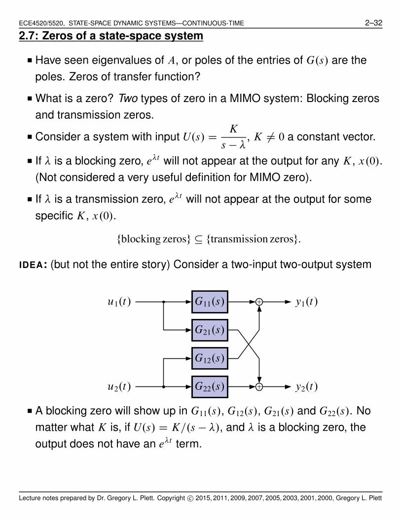
IDEA: (but not the entire story) Consider a two-input two-output system
u1.t/
u2.t/
y1.t/
y2.t/
G11.s/
G12.s/
G21.s/
G22.s/
■ A blocking zero will show up in G11.s/, G12.s/, G21.s/ and G22.s/. No
matter what K is, if U.s/ D K=.s ! $/, and $ is a blocking zero, the
output does not have an e$t term.
Lecture notes prepared by Dr. Gregory L. Plett. Copyright c" 2015, 2011, 2009, 2007, 2005, 2003, 2001, 2000, Gregory L. Plett
ECE4520/5520, STATE-SPACE DYNAMIC SYSTEMS—CONTINUOUS-TIME 2–33
■ A transmission zero may not show up as a zero in any of the
individual transfer functions, but will in combinations thereof (with
specific initial states).
■ To find transmission zeros, put in u.t/ D u0e´i t and you get a zero
output at “frequency” e´i t .
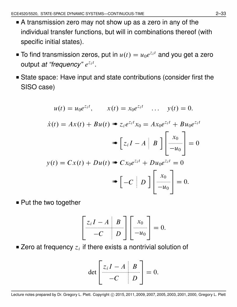
■ State space: Have input and state contributions (consider first the
SISO case)
u.t/ D u0e´i t ; x.t/ D x0e
´i t : : : y.t/ D 0:
Px.t/ D Ax.t/ C Bu.t/ ➠ ´ie´i tx0 D Ax0e
´i t C Bu0e´i t
➠
h
´iI ! A Bi
2
4
x0
!u0
3
5 D 0
y.t/ D Cx.t/ C Du.t/ ➠ Cx0e´i t C Du0e
´i t D 0
➠
h
!C Di
2
4
x0
!u0
3
5 D 0:
■ Put the two together
2
4´iI ! A B
!C D
3
5
2
4
x0
!u0
3
5 D 0:
■ Zero at frequency ´i if there exists a nontrivial solution of
det
2
4´iI ! A B
!C D
3
5 D 0:
Lecture notes prepared by Dr. Gregory L. Plett. Copyright c" 2015, 2011, 2009, 2007, 2005, 2003, 2001, 2000, Gregory L. Plett

ECE4520/5520, STATE-SPACE DYNAMIC SYSTEMS—CONTINUOUS-TIME 2–34
■ Recall
G.s/ D
det
2
4sI ! A B
!C D
3
5
det.sI ! A/:
Ahah! (The !u0 before gave us the correct sign in G.s/).
■ In the MIMO case, with n state variables, p inputs and q outputs, a
transmission zero is any value ´i for which
rank
2
4´iI ! A B
!C D
3
5 < n C minfp; qg
EXAMPLE:
G.s/ D
2
64
s.s C 1/
s2 C 1
s C 1
s C 2
0.s C 2/.s C 1/
s2 C 2s C 2
3
75 :
■ We can find that G.s/ has a blocking zero at s D !1 and has
transmission zeros at s D 0, s D !1 and s D !2.
Y1.s/ Ds.s C 1/
s2 C 1U1.s/ C
s C 1
s C 2U2.s/
Y2.s/ D.s C 2/.s C 1/
s2 C 2s C 2U2.s/:
Let U D K=.s ! $/
Y1.s/ Ds C 1
s ! $
%
s.s C 2/k1 C .s2 C 1/k2
.s2 C 1/.s C 2/
&
Y2.s/ Ds C 1
s ! $
%
.s C 2/k2
s2 C 2s C 2
&
:
Lecture notes prepared by Dr. Gregory L. Plett. Copyright c" 2015, 2011, 2009, 2007, 2005, 2003, 2001, 2000, Gregory L. Plett

ECE4520/5520, STATE-SPACE DYNAMIC SYSTEMS—CONTINUOUS-TIME 2–35
■ For all k1, k2, s D !1 is a zero. Therefore, both blocking and
transmission.
■ For k2 D 0, k1 2 R, s D 0 is a zero. Therefore, transmission.
■ Not so obvious, but s D !2 is also a zero. Therefore, transmission. [In
a MIMO system, we can have a zero and pole at the same frequency!]
■ Recall from before,2
4´iI ! A B
!C D
3
5
2
4
x0
!u0
3
5 D 0:
gives the initial state x0 and K D u0 if ´i is a transmission zero.
■ In MATLAB: tzero(sys)
Lecture notes prepared by Dr. Gregory L. Plett. Copyright c" 2015, 2011, 2009, 2007, 2005, 2003, 2001, 2000, Gregory L. Plett
ECE4520/5520, STATE-SPACE DYNAMIC SYSTEMS—CONTINUOUS-TIME 2–36
2.8: Linear time-varying systems
■ With relatively small changes in what we’ve seen, we can also model
linear time-varying (LTV) systems
Px.t/ D A.t/x.t/ C B.t/u.t/
y.t/ D C.t/x.t/ C D.t/u.t/:
■ LTV systems do not have transfer functions (so we cannot analyze in
the Laplace domain).
■ However, they do have (time varying) impulse responses.
■ Let g.t; !/ be the output signal from the system corresponding to an
input signal ı.t ! !/.
■ Then, the general output from a causal LTV system can be written as
y.t/ DZ 1
0
g.t; !/u.!/ d!:
Homogeneous response
■ To see responses of LTV state-space systems, consider first the
homogeneous case
Px.t/ D A.t/x.t/; x.t0/ D x0; t # 0:
FACT: The unique solution to this equation can be given by
x.t/ D ˆ.t; t0/x0; t # 0;
where the n & n state-transition matrix ˆ.t; t0/ is given by
ˆ.t; t0/ D I CZ t
t0
A.s1/ ds1 CZ t
t0
A.s1/
Z s1
t0
A.s2/ ds2 ds1
CZ t
t0
A.s1/
Z s1
t0
A.s2/
Z s2
t0
A.s3/ ds3 ds2 ds1 C % % %
Lecture notes prepared by Dr. Gregory L. Plett. Copyright c" 2015, 2011, 2009, 2007, 2005, 2003, 2001, 2000, Gregory L. Plett
ECE4520/5520, STATE-SPACE DYNAMIC SYSTEMS—CONTINUOUS-TIME 2–37
■ Some important properties of the state-transition matrix are:
1. P .t; t0/ D A.t/ˆ.t; t0/; ˆ.t0; t0/ D I; t # 0.
2. ˆ.t; s/ˆ.s; !/ D ˆ.t; !/.
3. ˆ.t; !/!1 D ˆ.!; t /.
■ To prove the first property, we start with
x.t/ D ˆ.t; t0/x0
Px.t/ D P .t; t0/x0 C ˆ.t; t0/ Px0„ ƒ‚ …
0
D A.t/x.t/:
■ So, we have
A.t/x.t/ D P .t; t0/x0
A.t/ˆ.t; t0/x0 D P .t; t0/x0:
■ Since this must be true for arbitrary x0, we have shown that
P .t; t0/ D A.t/ˆ.t; t0/:
■ The second property is easily shown by breaking up the time line into
the intervals from ! to s, and then from s to t .
x.s/ D ˆ.s; !/x.!/
x.t/ D ˆ.t; s/x.s/
x.t/ D ˆ.t; s/ˆ.s; !/„ ƒ‚ …
ˆ.t;!/
x.!/:
■ The third property relates to going backward in time from a final state
to an initial state.
x.t/ D ˆ.t; t0/x.t0/
x.t0/ D ˆ!1.t; t0/x.t/:
Lecture notes prepared by Dr. Gregory L. Plett. Copyright c" 2015, 2011, 2009, 2007, 2005, 2003, 2001, 2000, Gregory L. Plett
ECE4520/5520, STATE-SPACE DYNAMIC SYSTEMS—CONTINUOUS-TIME 2–38
■ For an LTI system, we have ˆ.t; t0/ D eA.t!t0/. So, this new
state-transition matrix is simply a generalization of what we have
already seen.
Forced response
■ Generalizing the prior result, we can find that the nonhomogeneous
state solution is
x.t/ D ˆ.t; t0/x0 CZ t
t0
ˆ.t; !/B.!/u.!/ d!:
■ To show this, start with the assumed answer and differentiate with
respect to time t
Px.t/ D P .t; t0/x0 CZ t
t0
P .t; !/B.!/u.!/ d! C ˆ.t; t/B.t/u.t/;
where we have needed Liebnitz’ rule for differentiating an integral,
which is
d
d'
Z b.'/
a.'/
f .x; '/ dx DZ b.'/
a.'/
@f .x; '/
@'dx C f .b.'/; '/
@b.'/
@'
! f .a.'/; '/@a.'/
@';
assuming that f .x; '/ is continuous and that the integral exists.
■ Using our known result for P .t; t0/ and the fact that ˆ.t; t/ D I ,
Px.t/ D A.t/ˆ.t; t0/x0 CZ t
t0
A.t/ˆ.t; !/B.!/u.!/ d! C B.t/u.t/:
■ Since the integral is with respect to !; we can factor out A.t/
Px.t/ D A.t/
#
ˆ.t; t0/x0 CZ t
t0
ˆ.t; !/B.!/u.!/ d!
$
C B.t/u.t/
D A.t/x.t/ C B.t/u.t/:
Lecture notes prepared by Dr. Gregory L. Plett. Copyright c" 2015, 2011, 2009, 2007, 2005, 2003, 2001, 2000, Gregory L. Plett
ECE4520/5520, STATE-SPACE DYNAMIC SYSTEMS—CONTINUOUS-TIME 2–39
■ Substituting into y.t/ D C.t/x.t/ C D.t/u.t/, we get
y.t/ D C.t/ˆ.t; t0/x0 CZ t
t0
C.t/ˆ.t; !/B.!/u.!/ d! C D.t/u.t/:
■ We can rewrite this as
y.t/ D C.t/ˆ.t; t0/x0 CZ t
t0
ŒC.t/ˆ.t; !/B.!/ C D.!/ı.t ! !/" u.!/ d!
D C.t/ˆ.t; t0/x0 CZ t
t0
h.t; !/u.!/ d!
which allows us to recognize the impulse response of a LTV system
to be
h.t; !/ D C.t/ˆ.t; !/B.!/ C D.!/ı.t ! !/:
Equivalent transformations for LTV systems
■ Transformations of LTV systems are usually time-varying.
■ Let T .t/ be nonsingular for all t and define
x.t/ D T .t/´.t/
such that
Px.t/ D PT .t/´.t/ C T .t/ P.t/ D A.t/T .t/´.t/ C B.t/u.t/:
■ Then, we have
T .t/ P.t/ D'
A.t/T .t/ ! PT .t/(
´.t/ C B.t/u.t/;
which gives the equivalent LTV system
P.t/ D T !1.t/'
A.t/T .t/ ! PT .t/(
´.t/ C T !1.t/B.t/u.t/
y.t/ D C.t/T .t/´.t/ C D.t/u.t/:
Lecture notes prepared by Dr. Gregory L. Plett. Copyright c" 2015, 2011, 2009, 2007, 2005, 2003, 2001, 2000, Gregory L. Plett
ECE4520/5520, STATE-SPACE DYNAMIC SYSTEMS—CONTINUOUS-TIME 2–40
■ A transformation matrix is called a fundamental matrix when it
annihilates the term in square brackets
PT .t/ D A.t/T .t/; T .t0/ ¤ 0:
■ In this case, then
P.t/ D T !1.t/B.t/u.t/
or
´.t/ D ´.t0/ CZ t
t0
T !1.!/B.!/u.!/ d!
and
x.t/ D T .t/´.t0/ CZ t
t0
T .t/T !1.!/B.!/u.!/ d!
D T .t/T !1.t0/x0 CZ t
t0
T .t/T !1.!/B.!/u.!/ d!
D ˆ.t; t0/x0 CZ t
t0
ˆ.t; !/B.!/u.!/ d!:
■ This gives us a practical way to compute the state-transition matrix
ˆ.t; !/ D T .t/T !1.!/:
EXAMPLE: Consider the LTV system
Px.t/ D
"
0 0
t 0
#
x:
■ This is equivalent to stating
Px1.t/ D 0
Px2.t/ D tx1.t/
orx1.t/ D x1.t0/
x2.t/ D x2.t0/ C1
2.t2 ! t 2
0 /x1.t0/:
Lecture notes prepared by Dr. Gregory L. Plett. Copyright c" 2015, 2011, 2009, 2007, 2005, 2003, 2001, 2000, Gregory L. Plett

ECE4520/5520, STATE-SPACE DYNAMIC SYSTEMS—CONTINUOUS-TIME 2–41
■ We wish to find a valid fundamental matrix T .t/, and from it find the
state-transition matrix ˆ.t; t0/.
■ So, we need to find any matrix T .t/ that satisfies
PT .t/ D A.t/T .t/; T .t0/ ¤ 0:
■ We choose to initialize the fundamental matrix T .0/ D I . This then
implies that if"
T11.0/
T21.0/
#
D
"
1
0
#
; then
"
T11.t/
T21.t/
#
D
2
4
11
2t2
3
5
and if"
T12.0/
T22.0/
#
D
"
0
1
#
; then
"
T12.t/
T22.t/
#
D
"
0
1
#
:
■ Combining these results as columns of T , we have
T .t/ D
2
4
1 01
2t2 1
3
5 :
■ You can verify that this matrix satisfies PT .t/ D A.t/T .t/.
■ Using this to find the state-transition matrix,
ˆ.t; t0/ D T .t/T !1.t0/
D
2
4
1 01
2t2 1
3
5
2
4
1 01
2t20 1
3
5
!1
D
2
4
1 01
2t2 1
3
5
2
4
1 0
!1
2t20 1
3
5 D
2
4
1 0
!1
2.t2 ! t 2
0 / 1
3
5 :
Lecture notes prepared by Dr. Gregory L. Plett. Copyright c" 2015, 2011, 2009, 2007, 2005, 2003, 2001, 2000, Gregory L. Plett

ECE4520/5520, STATE-SPACE DYNAMIC SYSTEMS—CONTINUOUS-TIME 2–42
2.9: What about nonlinear systems?
■ Nonlinear continuous-time state-space systems are modeled as
Px.t/ D f .x.t/; u.t//
y.t/ D g.x.t/; u.t//:
Linearizing around an equilibrium point
■ To work with nonlinear systems, using small input signals, we can
linearize these equations.
■ Suppose that there is an equilibrium constant solution
u.t/ D ueq; x.t/ D xeq; and y.t/ D yeq D g.xeq; ueq/;
that satisfies the nonlinear form.
■ Then, let the actual input signal and initial state be written as
u.t/ D ueq C ıu.t/; x.t0/ D xeq C ıxeq.t0/
for small ıu.t/.
■ Then, we can write actual state and output as
x.t/ D xeq C ıx.t/; y.t/ D yeq C ıy.t/:
■ Using the known form for y.t/, we have
ıy.t/ D g.x.t/; u.t// ! yeq
D g.xeq C ıx.t/; ueq C ıu.t// ! g.xeq; ueq/:
■ We expand the function g.%/ using Taylor-series around the
equilibrium point .xeq; ueq/
Lecture notes prepared by Dr. Gregory L. Plett. Copyright c" 2015, 2011, 2009, 2007, 2005, 2003, 2001, 2000, Gregory L. Plett
ECE4520/5520, STATE-SPACE DYNAMIC SYSTEMS—CONTINUOUS-TIME 2–43
g.xeq C ıx.t/; ueq C ıu.t// D g.xeq; ueq/ C#
dg.xeq; ueq/
dx
$
ıx.t/
C#
dg.xeq; ueq/
du
$
ıu.t/ C h:o:t:
■ Substituting into our result for ıy.t/,
ıy.t/ )#
dg.xeq; ueq/
dx
$
„ ƒ‚ …
C
ıx.t/ C#
dg.xeq; ueq/
du
$
„ ƒ‚ …
D
ıu.t/:
■ To determine the evolution of ıx, we first take its derivative
ı Px.t/ D Px.t/ D f .xeq C ıx; ueq C ıu/:
■ By Taylor series,
ı Px.t/ D#
df .xeq; ueq/
dx
$
„ ƒ‚ …
A
ıx.t/ C#
df .xeq; ueq/
du
$
„ ƒ‚ …
B
ıu.t/:
■ To summarize, the linearized perturbation system is
ı Px.t/ D Aıx.t/ C Bıu.t/
ıy.t/ D Cıx.t/ C Dıu.t/
and the overall state and output can be computed as
x.t/ D xeq C ıx.t/ and y.t/ D yeq C ıy.t/:
Linearizing around a trajectory
■ Instead of linearizing around an equilibrium point, which requires
small ıu.t/, we can also choose to linearize around a known solution
trajectory.
Lecture notes prepared by Dr. Gregory L. Plett. Copyright c" 2015, 2011, 2009, 2007, 2005, 2003, 2001, 2000, Gregory L. Plett

ECE4520/5520, STATE-SPACE DYNAMIC SYSTEMS—CONTINUOUS-TIME 2–44
■ Suppose it is known that
usol.t/; xsol.t/; ysol.t/
form a time-varying solution to the nonlinear dynamics of the system.
■ This means that
Pxsol.t/ D f .xsol.t/; usol.t//
ysol.t/ D g.xsol.t/; usol.t//:
■ Then, let general input, state, and output be
u.t/ D usol.t/ C ıu.t/
x.t/ D xsol.t/ C ıx.t/
y.t/ D ysol.t/ C ıy.t/:
■ Proceeding as before,
Px.t/ D Pxsol.t/ C ı Px.t/
ı Px.t/ D Px.t/ ! Pxsol.t/
D f .xsol.t/ C ıx.t/; usol.t/ C ıu.t// ! f .xsol.t/; usol.t//:
■ Using Taylor series,
ı Px.t/ )#
df .xsol; usol/
dx.t/
$
„ ƒ‚ …
A.t/
ıx.t/ C#
df .xsol; usol/
du.t/
$
„ ƒ‚ …
B.t/
ıu.t/
ıy.t/ )#
dg.xsol; usol/
dx.t/
$
„ ƒ‚ …
C.t/
ıx.t/ C#
dg.xsol; usol/
du.t/
$
„ ƒ‚ …
D.t/
ıu.t/:
Lecture notes prepared by Dr. Gregory L. Plett. Copyright c" 2015, 2011, 2009, 2007, 2005, 2003, 2001, 2000, Gregory L. Plett
ECE4520/5520, STATE-SPACE DYNAMIC SYSTEMS—CONTINUOUS-TIME 2–45
■ To summarize, the linearized perturbation system is
ı Px.t/ D A.t/ıx.t/ C B.t/ıu.t/
ıy.t/ D C.t/ıx.t/ C D.t/ıu.t/
and the overall state and output can be computed as
x.t/ D xsol C ıx.t/ and y.t/ D ysol C ıy.t/:
■ Notice that even if the nonlinear system is time-invariant, the
linearized system will be time-varying, in general.
Where to from here?
■ We have now seen how to model continuous-time LTI, LTV, and
nonlinear systems in state-space form.
■ We have seen some ways to analyze and predict system behaviors.
■ Our next step is to repeat this approach with discrete-time systems.
■ We will see that the results are very similar, which will allow us to use
common frameworks to develop deeper insights into state-space
systems and to synthesize controllers.
Lecture notes prepared by Dr. Gregory L. Plett. Copyright c" 2015, 2011, 2009, 2007, 2005, 2003, 2001, 2000, Gregory L. Plett
Recommended