
Staff Development Staff Development DazeDazeJune 27 & 28June 27 & 28
Tony GauvinTony Gauvin

ScheduleSchedule
Monday June 27 Monday June 27 9:00 – 12:00 9:00 – 12:00 Basic ExcelBasic Excel 12:00 – 1:00 Lunch for all workshop participants12:00 – 1:00 Lunch for all workshop participants 1:00 – 4:00 Advanced Excel1:00 – 4:00 Advanced Excel
Tuesday June 28Tuesday June 28 9:00 – 12:00 Basic Access9:00 – 12:00 Basic Access 12:00 – 1:00 Lunch for all workshop participants12:00 – 1:00 Lunch for all workshop participants 1:00 – 4:00 Advanced Access1:00 – 4:00 Advanced Access
Thursday June 30 Thursday June 30 Time TBA (2hrs.) Outlook HighlightsTime TBA (2hrs.) Outlook Highlights
All materials available at All materials available at http://perleybrook.umfk.maine.eduhttp://perleybrook.umfk.maine.edu

Working with computersWorking with computers
Some basic rulesSome basic rules1.1. Computers are stupid!Computers are stupid!2.2. Computers do exactly what you tell them to do Computers do exactly what you tell them to do
because of rule 1because of rule 13.3. If you get a wrong answer or result it is because If you get a wrong answer or result it is because
you gave the computer bad data or bad you gave the computer bad data or bad instructions (GIGO)instructions (GIGO)
4.4. Most applications have self-help features, use Most applications have self-help features, use themthem
1.1. Hit F1Hit F12.2. Look for “?”Look for “?”3.3. Top–right corner of application or toolbarTop–right corner of application or toolbar

Difference between Difference between Spreadsheets and Spreadsheets and DatabasesDatabases Spreadsheets (Excel) are electronic Spreadsheets (Excel) are electronic
ledgersledgers Store, manipulate and present numbersStore, manipulate and present numbers
Databases (Access) are electronic file Databases (Access) are electronic file cabinetscabinets Receive, store, organize and present dataReceive, store, organize and present data
Use the right applicationUse the right application Save time and effortSave time and effort Decrease frustrationDecrease frustration

Quick history of Quick history of spreadsheetsspreadsheets
1978 – 1978 – Robert Frankston & Dan Bricklin invented VisiCalc, the first spreadsheet. It came Robert Frankston & Dan Bricklin invented VisiCalc, the first spreadsheet. It came
out with the Apple II computer. VisiCalc did very well in its first year because it out with the Apple II computer. VisiCalc did very well in its first year because it could run. On personal computers, could perform simple math formulas, and gave could run. On personal computers, could perform simple math formulas, and gave immediate results.immediate results.
1983 1983 Lotus 123 was introduced. It allowed people to chart information and identify cells. Lotus 123 was introduced. It allowed people to chart information and identify cells.
For example cell A1.For example cell A1. 19851985
Lotus 123 number 2.Lotus 123 number 2. 1987 1987
New spreadsheet programs such as Excel and Corel Quattro Pro were introduced. New spreadsheet programs such as Excel and Corel Quattro Pro were introduced. This allowed people to add graphics. They are different because they include This allowed people to add graphics. They are different because they include graphic capabilities.graphic capabilities.
20012001 Spreadsheet programs in use today are Excel, Appleworks, Filemaker, and Corel Spreadsheet programs in use today are Excel, Appleworks, Filemaker, and Corel
Quattro Pro.Quattro Pro.
Source: http://library.thinkquest.org/J0110054/History.html

The Spreadsheet The Spreadsheet abstractionabstraction
An (near) infinite series of rows and columns An (near) infinite series of rows and columns called called CellsCells that that Store numbers (and other stuff)Store numbers (and other stuff) Store formulas that use other information in other Store formulas that use other information in other
cells and produce a results to be displayedcells and produce a results to be displayed A bunch of other neat stuffA bunch of other neat stuff
FormattingFormatting Charting Charting What-if scenariosWhat-if scenarios

Basic ExcelBasic Excel
To learn Excel we will build a simple To learn Excel we will build a simple worksheet (Microsoft’s name for spread worksheet (Microsoft’s name for spread sheet) sheet)
Advanced Excel Advanced Excel (afternoon)(afternoon)
TopicsTopics Formulas and FunctionsFormulas and Functions FormattingFormatting Importing and exporting dataImporting and exporting data Working with Large Spread SheetsWorking with Large Spread Sheets Anything else anyone wants to coverAnything else anyone wants to cover

Excel Project 1Excel Project 1
Creating a Worksheet Creating a Worksheet and an Embedded Chartand an Embedded Chart

ObjectivesObjectives
Start and Quit ExcelStart and Quit Excel Describe the Excel worksheetDescribe the Excel worksheet Enter text and numbersEnter text and numbers Use the AutoSum button to sum a range Use the AutoSum button to sum a range
of cellsof cells

ObjectivesObjectives
Copy a cell to a range of cells using the Copy a cell to a range of cells using the fill handlefill handle
Format a worksheetFormat a worksheet Create a 3-D Clustered column chartCreate a 3-D Clustered column chart Save a workbook and print a worksheetSave a workbook and print a worksheet

ObjectivesObjectives
Open a workbookOpen a workbook Use the AutoCalculate area to determine Use the AutoCalculate area to determine
statisticsstatistics Correct errors on a worksheetCorrect errors on a worksheet Use the Excel Help system to answer Use the Excel Help system to answer
questionsquestions

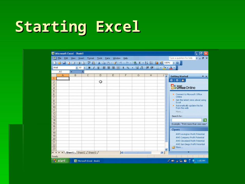
Starting ExcelStarting Excel
Click the Start button on the Windows Click the Start button on the Windows taskbar, point to All Programs on the taskbar, point to All Programs on the Start menu, point to Microsoft Office on Start menu, point to Microsoft Office on the All Programs submenu, and then the All Programs submenu, and then point to Microsoft Office Excel 2003 on point to Microsoft Office Excel 2003 on the Microsoft Office submenuthe Microsoft Office submenu
Click Microsoft Office Excel 2003Click Microsoft Office Excel 2003 If the Excel window is not maximized, If the Excel window is not maximized,
double-click its title bar to maximize itdouble-click its title bar to maximize it
Starting ExcelStarting Excel
Customizing the Excel Customizing the Excel WindowWindow
Right-click the Language barRight-click the Language bar Click Close the Language barClick Close the Language bar Click the Getting Started task pane Close Click the Getting Started task pane Close
button in the upper-right corner of the task button in the upper-right corner of the task panepane
If the toolbars are positioned on the same If the toolbars are positioned on the same row, click the Toolbar Options buttonrow, click the Toolbar Options button
Click Show Buttons on Two RowsClick Show Buttons on Two Rows
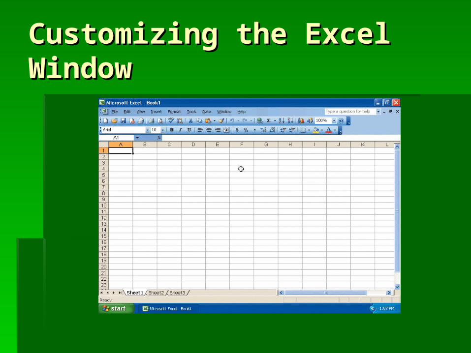
Customizing the Excel Customizing the Excel WindowWindow

Entering the Worksheet Entering the Worksheet TitlesTitles
Click cell A1Click cell A1 Type Type Extreme BladingExtreme Blading in cell A1 and in cell A1 and
then point to the Enter box in the formula barthen point to the Enter box in the formula bar Click the Enter button to complete the entryClick the Enter button to complete the entry Click cell A2 to select it. Type Click cell A2 to select it. Type Second Second Quarter SalesQuarter Sales as the cell entry. Click the as the cell entry. Click the Enter box to complete the entryEnter box to complete the entry

Entering the Worksheet Entering the Worksheet TitlesTitles

Entering Column TitlesEntering Column Titles
Click cell B3Click cell B3 Type Type Direct MailDirect Mail in cell B3 in cell B3 Press the RIGHT ARROW keyPress the RIGHT ARROW key Repeat the last two steps for the Repeat the last two steps for the
remaining column titles in row 3, as remaining column titles in row 3, as shown on the following slideshown on the following slide

Entering Column TitlesEntering Column Titles

Entering Row TitlesEntering Row Titles
Click cell A4. Type Click cell A4. Type Inline SkatesInline Skates and then press the DOWN ARROW keyand then press the DOWN ARROW key
Repeat the previous step for the Repeat the previous step for the remaining row titles in column A, as remaining row titles in column A, as shown on the following slideshown on the following slide

Entering Row TitlesEntering Row Titles

Entering NumbersEntering Numbers
Click cell B4Click cell B4 Type Type 58835.3558835.35 and then press the RIGHT and then press the RIGHT
ARROW keyARROW key Enter Enter 97762.5097762.50 in cell C4, in cell C4, 71913.7371913.73 in cell in cell
D4, and D4, and 85367.3785367.37 in cell E4 in cell E4 Click cell B5Click cell B5 Enter the remaining fourth quarter sales Enter the remaining fourth quarter sales
provided on the next slide for each of the three provided on the next slide for each of the three remaining product groups in rows 5, 6, and 7remaining product groups in rows 5, 6, and 7

Entering NumbersEntering Numbers
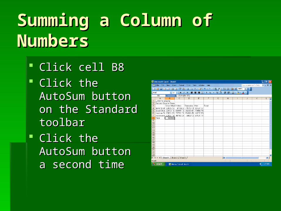
Summing a Column of Summing a Column of NumbersNumbers
Click cell B8Click cell B8 Click the AutoSum Click the AutoSum
button on the button on the Standard toolbarStandard toolbar
Click the AutoSum Click the AutoSum button a second timebutton a second time
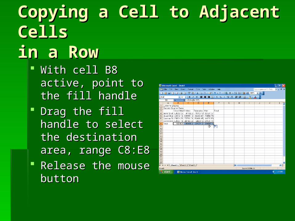
Copying a Cell to Adjacent Copying a Cell to Adjacent Cells Cells in a Rowin a Row
With cell B8 active, With cell B8 active, point to the fill handlepoint to the fill handle
Drag the fill handle to Drag the fill handle to select the destination select the destination area, range C8:E8area, range C8:E8
Release the mouse Release the mouse buttonbutton

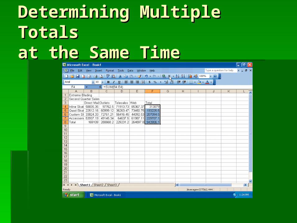
Determining Multiple Determining Multiple Totals Totals at the Same Timeat the Same Time
Click cell F4Click cell F4 With the mouse pointer in cell F4 and in With the mouse pointer in cell F4 and in
the shape of a block plus sign, drag the the shape of a block plus sign, drag the mouse pointer down to cell F8mouse pointer down to cell F8
Click the AutoSum button on the Click the AutoSum button on the Standard toolbarStandard toolbar
Select cell A9 to deselect the range Select cell A9 to deselect the range F4:F8F4:F8
Determining Multiple Determining Multiple Totals Totals at the Same Timeat the Same Time

Changing the Font TypeChanging the Font Type
Click cell A1 and then point to the Font Click cell A1 and then point to the Font box arrow on the Formatting toolbarbox arrow on the Formatting toolbar
Click the Font box arrow and then point Click the Font box arrow and then point to Arial Rounded MT Boldto Arial Rounded MT Bold
Click Arial Rounded MT BoldClick Arial Rounded MT Bold

Changing the Font TypeChanging the Font Type

Bolding a CellBolding a Cell
With cell A1 active, click the Bold button With cell A1 active, click the Bold button on the Formatting toolbaron the Formatting toolbar

Increasing the Font Size Increasing the Font Size of a Cell Entryof a Cell Entry
With cell A1 selected, With cell A1 selected, click the Font Size click the Font Size box arrow on the box arrow on the Formatting toolbar Formatting toolbar
Click 24 in the Font Click 24 in the Font Size listSize list

Changing the Font Color Changing the Font Color of a Cell Entryof a Cell Entry
With cell A1 selected, With cell A1 selected, click the Font Color click the Font Color button arrow on the button arrow on the Formatting toolbarFormatting toolbar
Click Violet (column Click Violet (column 7, row 3) on the Font 7, row 3) on the Font Color paletteColor palette
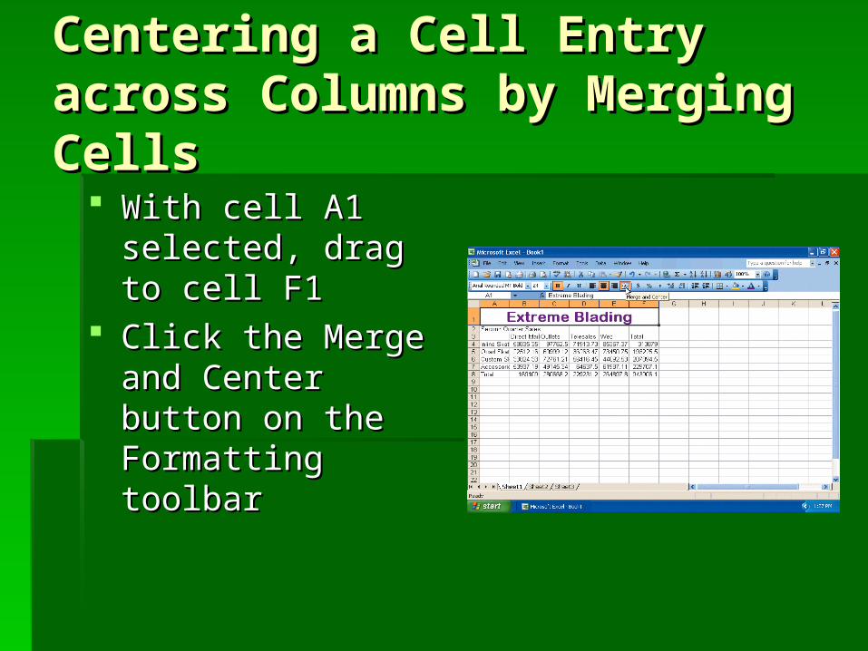
Centering a Cell Entry Centering a Cell Entry across Columns by Merging across Columns by Merging CellsCells
With cell A1 selected, With cell A1 selected, drag to cell F1drag to cell F1
Click the Merge and Click the Merge and Center button on the Center button on the Formatting toolbarFormatting toolbar

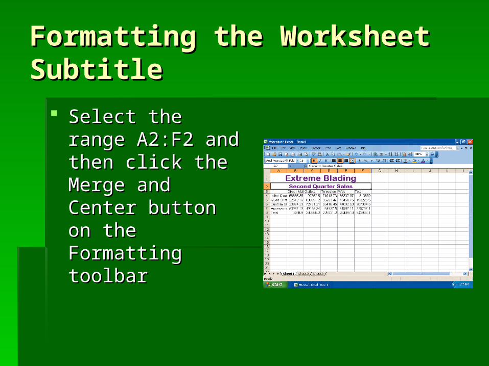
Formatting the Worksheet Formatting the Worksheet SubtitleSubtitle
Select cell A2Select cell A2 Click the Font box arrow on the Formatting Click the Font box arrow on the Formatting
toolbar and then click Arial Rounded MT Boldtoolbar and then click Arial Rounded MT Bold Click the Bold button on the Formatting toolbarClick the Bold button on the Formatting toolbar Click the Font Size box arrow on the Click the Font Size box arrow on the
Formatting toolbar and then click 16Formatting toolbar and then click 16 Click the Font Color button on the Formatting Click the Font Color button on the Formatting
toolbartoolbar
Formatting the Worksheet Formatting the Worksheet SubtitleSubtitle
Select the range Select the range A2:F2 and then click A2:F2 and then click the Merge and the Merge and Center button on the Center button on the Formatting toolbarFormatting toolbar

Using AutoFormat to Using AutoFormat to Format Format the Body of a Worksheetthe Body of a Worksheet
Select cell A3, the upper-left corner cell of Select cell A3, the upper-left corner cell of the rectangular range to formatthe rectangular range to format
Drag the mouse pointer to cell F8, the Drag the mouse pointer to cell F8, the lower-right corner cell of the range to lower-right corner cell of the range to formatformat
Click Format on the menu barClick Format on the menu bar Click AutoFormat on the Format menuClick AutoFormat on the Format menu When Excel displays the AutoFormat When Excel displays the AutoFormat
dialog box, click the Accounting 2 formatdialog box, click the Accounting 2 format

Using AutoFormat to Using AutoFormat to Format Format the Body of a Worksheetthe Body of a Worksheet
Click the OK buttonClick the OK button Select cell A10 to Select cell A10 to
deselect the range deselect the range A3:F8A3:F8
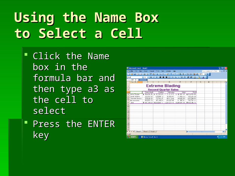
Using the Name Box Using the Name Box to Select a Cellto Select a Cell
Click the Name box Click the Name box in the formula bar in the formula bar and then type and then type a3a3 as as the cell to selectthe cell to select
Press the ENTER Press the ENTER keykey


Adding a 3-D Clustered Adding a 3-D Clustered Column Chart to the Column Chart to the WorksheetWorksheet
With cell A3 selected, position the block plus sign With cell A3 selected, position the block plus sign mouse pointer within the cell’s border and drag the mouse pointer within the cell’s border and drag the mouse pointer to the lower-right corner cell (cell E7) of mouse pointer to the lower-right corner cell (cell E7) of the range to chart (A3:E7the range to chart (A3:E7
Click the Chart Wizard button on the Standard toolbarClick the Chart Wizard button on the Standard toolbar When Excel displays the Chart Wizard – Step 1 of 4 – When Excel displays the Chart Wizard – Step 1 of 4 –
Chart Type dialog box and with Column selected in the Chart Type dialog box and with Column selected in the Chart style list, click Clustered column with a 3-D visual Chart style list, click Clustered column with a 3-D visual effect (column 1, row 2) in the Chart sub-type areaeffect (column 1, row 2) in the Chart sub-type area
Click the Finish buttonClick the Finish button If the Chart toolbar appears, click its Close buttonIf the Chart toolbar appears, click its Close button

Adding a 3-D Clustered Adding a 3-D Clustered Column Chart to the Column Chart to the WorksheetWorksheet
When Excel displays the chart, point to an When Excel displays the chart, point to an open area in the lower-right section of the chart open area in the lower-right section of the chart area so the ScreenTip, Chart Area, appears area so the ScreenTip, Chart Area, appears next to the mouse pointernext to the mouse pointer
Drag the chart down and to the left to position Drag the chart down and to the left to position the upper-left corner of the dotted line the upper-left corner of the dotted line rectangle over the upper-left corner of cell A10rectangle over the upper-left corner of cell A10
Release the mouse buttonRelease the mouse button Point to the middle sizing handle on the right Point to the middle sizing handle on the right
edge of the selection rectangleedge of the selection rectangle
Adding a 3-D Clustered Adding a 3-D Clustered Column Chart to the Column Chart to the WorksheetWorksheet
While holding down the ALT key, drag While holding down the ALT key, drag the sizing handle to the right edge of the sizing handle to the right edge of column Fcolumn F
If necessary, hold down the ALT key and If necessary, hold down the ALT key and drag the lower-middle sizing handle down drag the lower-middle sizing handle down to the bottom border of row 20to the bottom border of row 20
Click cell H20 to deselect the chartClick cell H20 to deselect the chart

Adding a 3-D Clustered Adding a 3-D Clustered Column Chart to the Column Chart to the WorksheetWorksheet

Saving a WorkbookSaving a Workbook
With a floppy disk in drive A, click the With a floppy disk in drive A, click the Save button on the Standard toolbarSave button on the Standard toolbar
Type Type Extreme Blading 2nd Quarter Extreme Blading 2nd Quarter SalesSales in the File name box in the File name box
Click the Save in box arrowClick the Save in box arrow Click 3½ Floppy (A:) in the Save in listClick 3½ Floppy (A:) in the Save in list Click the Save button in the Save As Click the Save button in the Save As
dialog boxdialog box

Saving a WorkbookSaving a Workbook

Printing a WorksheetPrinting a Worksheet
Ready the printer Ready the printer according to the according to the printer instructions printer instructions and then click the and then click the Print button on the Print button on the Standard toolbarStandard toolbar
When the printer When the printer stops printing the stops printing the worksheet and the worksheet and the chart, retrieve the chart, retrieve the printoutprintout

Quitting ExcelQuitting Excel
Point to the Close Point to the Close button on the right button on the right side of the title barside of the title bar
Click the Close Click the Close buttonbutton
Click the No buttonClick the No button

Starting Excel Starting Excel and Opening a Workbookand Opening a Workbook
With your floppy disk in drive A, click the Start With your floppy disk in drive A, click the Start button on the Windows taskbar, point to All button on the Windows taskbar, point to All Programs on the Start menu, point to Microsoft Programs on the Start menu, point to Microsoft Office on the All Programs submenu, and then Office on the All Programs submenu, and then click Microsoft Office Excel 2003 on the click Microsoft Office Excel 2003 on the Microsoft Office submenuMicrosoft Office submenu
Click Extreme Blading 2nd Quarter Sales in the Click Extreme Blading 2nd Quarter Sales in the Open area in the Getting Started task paneOpen area in the Getting Started task pane

Starting Excel Starting Excel and Opening a Workbookand Opening a Workbook

Using the AutoCalculate Using the AutoCalculate Area to Determine an Area to Determine an AverageAverage
Select the range B6:E6 and then right-Select the range B6:E6 and then right-click the AutoCalculate area on the status click the AutoCalculate area on the status barbar
Click Average on the shortcut menuClick Average on the shortcut menu Right-click the AutoCalculate area and Right-click the AutoCalculate area and
then click Sum on the shortcut menuthen click Sum on the shortcut menu

Using the AutoCalculate Using the AutoCalculate Area to Determine an Area to Determine an AverageAverage
Clearing Cell ContentsClearing Cell Contents
Fill HandleFill Handle Select the cell or range of cells and point to the fill Select the cell or range of cells and point to the fill
handle so the mouse pointer changes to a cross hairhandle so the mouse pointer changes to a cross hair Drag the fill handle back into the selected cell or Drag the fill handle back into the selected cell or
range until a shadow covers the cell or cells you range until a shadow covers the cell or cells you want to erase. Release the mouse buttonwant to erase. Release the mouse button
Shortcut MenuShortcut Menu Select the cell or range of cells to be clearedSelect the cell or range of cells to be cleared Right-click the selectionRight-click the selection Click Clear Contents on the shortcut menuClick Clear Contents on the shortcut menu

Clearing Cell ContentsClearing Cell Contents
Delete KeyDelete Key Select the cell or range of cells to be clearedSelect the cell or range of cells to be cleared Press the DELETE keyPress the DELETE key
Clear CommandClear Command Select the cell or range of cells to be clearedSelect the cell or range of cells to be cleared Click Edit on the menu bar and then point to Click Edit on the menu bar and then point to
ClearClear Click All on the Clear submenuClick All on the Clear submenu
Clearing the Entire Clearing the Entire WorksheetWorksheet
Click the Select All button on the Click the Select All button on the worksheetworksheet
Press the DELETE key or click Edit on Press the DELETE key or click Edit on the menu bar, point to Clear and then the menu bar, point to Clear and then click All on the Clear submenuclick All on the Clear submenu
Deleting an Embedded Deleting an Embedded ChartChart
Click the chart to select itClick the chart to select it Press the DELETE keyPress the DELETE key
Obtaining Help Obtaining Help Using the Type a Question for Using the Type a Question for Help BoxHelp Box
Type Type save a workbooksave a workbook in the Type a Question for in the Type a Question for help box on the right side of the menu barhelp box on the right side of the menu bar
Press the ENTER keyPress the ENTER key When Excel displays the Search Results task pane, When Excel displays the Search Results task pane,
scroll down and then click the link Save a filescroll down and then click the link Save a file If necessary, click the AutoTile button to tile the If necessary, click the AutoTile button to tile the
windowswindows Click the Show All link on the right side of the Click the Show All link on the right side of the
Microsoft Excel Help window to expand the links in Microsoft Excel Help window to expand the links in the windowthe window

Obtaining Help Obtaining Help Using the Type a Question for Using the Type a Question for Help BoxHelp Box
Double-click the Microsoft Excel Help title Double-click the Microsoft Excel Help title bar to maximize itbar to maximize it
Click the Close button on the Microsoft Click the Close button on the Microsoft Excel Help window title barExcel Help window title bar

Obtaining Help Obtaining Help Using the Type a Question for Using the Type a Question for Help BoxHelp Box

Quitting ExcelQuitting Excel
Click the Close button on the right side of Click the Close button on the right side of the title bar, and if necessary, click the the title bar, and if necessary, click the No button in the Microsoft Excel dialog No button in the Microsoft Excel dialog boxbox

SummarySummary
Start and Quit ExcelStart and Quit Excel Describe the Excel worksheetDescribe the Excel worksheet Enter text and numbersEnter text and numbers Use the AutoSum button to sum a range Use the AutoSum button to sum a range
of cellsof cells Copy a cell to a range of cells using the Copy a cell to a range of cells using the
fill handlefill handle
SummarySummary
Copy a cell to a range of cells using the Copy a cell to a range of cells using the fill handlefill handle
Format a worksheetFormat a worksheet Create a 3-D Clustered column chartCreate a 3-D Clustered column chart Save a workbook and print a worksheetSave a workbook and print a worksheet

SummarySummary
Open a workbookOpen a workbook Use the AutoCalculate area to determine Use the AutoCalculate area to determine
statisticsstatistics Correct errors on a worksheetCorrect errors on a worksheet Use the Excel Help system to answer Use the Excel Help system to answer
questionsquestions

Questions??Questions??
Recommended


![Super! drama TV June 2020 · Super! drama TV June 2020 Note: #=serial number [J]=in Japanese 27:30 28:00 28:30 29:00 21:30 22:00 22:30 23:00 Programs are subject to change without](https://img.dokumen.tips/doc/110x75/5f8946a95bc32f7e016563d8/super-drama-tv-june-super-drama-tv-june-2020-note-serial-number-jin-japanese.jpg)

