Spherical Harmonic Lighting
Nivedita Goswami
Master of Science
Computer Animation and Visual Effects
Bournemouth University, Poole, Dorset, United Kingdom. August, 2013

Contents
Table of contents . . . . . . . . . . . . . . . . . . . . . . . . . . . . . . . . . . . .i
Abstract . . . . . . . . . . . . . . . . . . . . . . . . . . . . . . . . . . . . . . . . . iii
1 Introduction 1
1.1 Objective . . . . . . . . . . . . . . . . . . . . . . . . . . . . . . . . . . . . . 1
1.2 Motivation . . . . . . . . . . . . . . . . . . . . . . . . . . . . . . . . . . . . . 1
1.3 Structure . . . . . . . . . . . . . . . . . . . . . . . . . . . . . . . . . . . . . . 3
2 Background and Related Work 4
2.1 Illumination . . . . . . . . . . . . . . . . . . . . . . . . . . . . . . . . . . . . 4
2.1.1 Direct Light or Local Illumination . . . . . . . . . . . . . . . .. . . . 4
2.1.2 Indirect Light or Global Illumination . . . . . . . . . . . . .. . . . . 5
2.1.3 The Rendering Equation and Radiosity . . . . . . . . . . . . . .. . . 6
2.2 RenderMan . . . . . . . . . . . . . . . . . . . . . . . . . . . . . . . . . . . . 8
3 Spherical Harmonics 10
3.1 Orthogonal basis functions . . . . . . . . . . . . . . . . . . . . . . . .. . . . 10
3.2 Spherical Harmonics . . . . . . . . . . . . . . . . . . . . . . . . . . . . . .. 13
3.3 Spherical Harmonic Projection . . . . . . . . . . . . . . . . . . . . .. . . . . 14
3.4 Properties of SH functions . . . . . . . . . . . . . . . . . . . . . . . . .. . . 15
4 Implementation 17
4.1 C++ Test Bench . . . . . . . . . . . . . . . . . . . . . . . . . . . . . . . . . . 17
4.2 Dynamic Shared Object . . . . . . . . . . . . . . . . . . . . . . . . . . . . .. 17
4.3 RenderMan Workflow . . . . . . . . . . . . . . . . . . . . . . . . . . . . . . . 19
4.4 simpleBake.sl . . . . . . . . . . . . . . . . . . . . . . . . . . . . . . . . . . .19
i

4.5 shBasis.sl . . . . . . . . . . . . . . . . . . . . . . . . . . . . . . . . . . . . . 20
4.6 shProjection.sl . . . . . . . . . . . . . . . . . . . . . . . . . . . . . . . . .. . 21
4.7 shLight.sl . . . . . . . . . . . . . . . . . . . . . . . . . . . . . . . . . . . . . 23
4.7.1 Types of Light . . . . . . . . . . . . . . . . . . . . . . . . . . . . . . 23
5 Results and Analysis 25
5.1 Efficiency . . . . . . . . . . . . . . . . . . . . . . . . . . . . . . . . . . . . . 25
5.2 Quality . . . . . . . . . . . . . . . . . . . . . . . . . . . . . . . . . . . . . . 26
5.3 Examples and Comparisons . . . . . . . . . . . . . . . . . . . . . . . . . .. . 28
5.3.1 SH Direct . . . . . . . . . . . . . . . . . . . . . . . . . . . . . . . . . 28
5.3.2 SH Indirect . . . . . . . . . . . . . . . . . . . . . . . . . . . . . . . . 30
6 Conclusion 34
6.1 Summary . . . . . . . . . . . . . . . . . . . . . . . . . . . . . . . . . . . . . 34
6.2 Discussion . . . . . . . . . . . . . . . . . . . . . . . . . . . . . . . . . . . . . 34
6.3 Future work . . . . . . . . . . . . . . . . . . . . . . . . . . . . . . . . . . . . 35
References 35
ii
Abstract
The rendering of objects under distant diffuse illumination has been considered. The illumi-
nation has been projected into spherical harmonic space andthe coefficients are stored in the
geometry to reconstruct the lighting. RenderMan has been the choice of platform for the im-
plementation. Using a plugin, the existing functionality of RenderMan has been extended to
make it capable of spherical harmonic lighting.
iii

Chapter 1
Introduction
1.1 Objective
The objective of this project is to use Spherical Harmonics (SH) for illumination calculations.
Using comparative examples, the thesis will demonstrate the advantages of this precomputation
technique over standard ray trace lighting in terms of both efficiency and quality.
Photo Realistic RenderMan (PRMan), the well established renderer from Pixar, has been
used for the project. The functionality of the renderer has been extended to make it capable
of computing spherical harmonic data and some of the standard lights have been extended to
make them capable of spherical harmonic lighting.
1.2 Motivation
The general drive in computer graphics is to achieve better and more believable imagery and to
achieve them within feasible time frames. An obvious solution is better hardware but a more
beneficial solution would be to have software that uses efficient calculations and can also be
incorporated as an artist-friendly tool within the production pipeline.
PantaRay, the novel system for precomputing directional occlusion caches developed by
Weta Digital and Nvidia for the production of the feature filmAvatar, is an influential example
1
of accelerating cinematic lighting in the domain of spherical harmonics.
The movie Avatar featured unprecedented geometric complexity, with production shots con-
taining anywhere from ten million to over one billion polygons (Pantaleoni et al. 2010). Re-
lighting methods based on spherical harmonics (Ramamoorthi & Hanrahan 2001a) and image-
based lighting made it possible to render such complex scenes and to provide artists with fast
iterations for lighting.
The key feature of PantaRay is to make the expensive precomputation of spherical harmon-
ics practical by implementing ray tracing calculations on the GPU and generating directional
occlusion caches. A GPU implementation is beyond the scope of this thesis, but the idea of
precomputed caches has been used for this project.
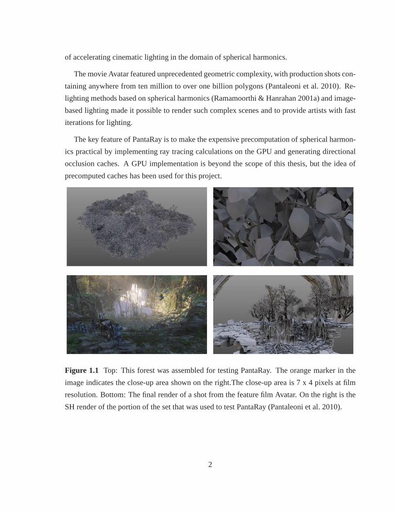
Figure 1.1 Top: This forest was assembled for testing PantaRay. The orange marker in the
image indicates the close-up area shown on the right.The close-up area is 7 x 4 pixels at film
resolution. Bottom: The final render of a shot from the feature film Avatar. On the right is the
SH render of the portion of the set that was used to test PantaRay (Pantaleoni et al. 2010).
2
1.3 Structure
The structure of this thesis follows the sequence of steps undertaken to understand the concepts
behind the topic and then to implement them as a test bench in C++. It then moves on to PRMan
shaders followed by examples.
Chapter 2 introduces the background knowledge that is vitalbefore progressing to the partic-
ular topic of Spherical Harmonics. The principles of illumination in CG have been described.
The general principles of rendering and the working conceptbehind Prman has been discussed.
The project requires a thorough understanding of the mathematics behind Spherical Har-
monics and hence Chapter 3 deals with the fundamentals of SH.It defines SH functions, their
properties and the application of SH functions in lighting.
The implementation is described in Chapter 4. The evaluation of spherical harmonic func-
tions is tested in stand alone C++ using known light equations coefficients. The tested and
verified C++ code is then modified to a RenderMan Shading Language (RSL) Plugin that can
be called by a shader as a Dynamic Shared Object (DSO). The shaders that execute the neces-
sary task of pre-baking data are discussed and then a light shader that reads in the pre-processed
data is described. The extended SH versions of some of the standard lights in PRMan have also
been demonstrated.
The results obtained from using SH lighting are compared with standard techniques in Chap-
ter 5. Statistical demonstrations along with the renders are shown to illustrate the advantages
of Spherical Harmonic Ligting. To further demonstrate the robustness of the extended SH light
shaders a couple of examples dealing with complex geometry and different lighting conditions
have been used.
Finally, Chapter 6 presents a summary of the project and discusses its shortcomings. It also
presents several suggestions for further improvement of the tool and a better integration of it in
the production pipeline.
3
Chapter 2
Background and Related Work
2.1 Illumination
Light propagation and interaction with surface materials is a complex process and several light-
ing model have been developed in CG to represent the behaviour of light and the way it interacts
with different surfaces.
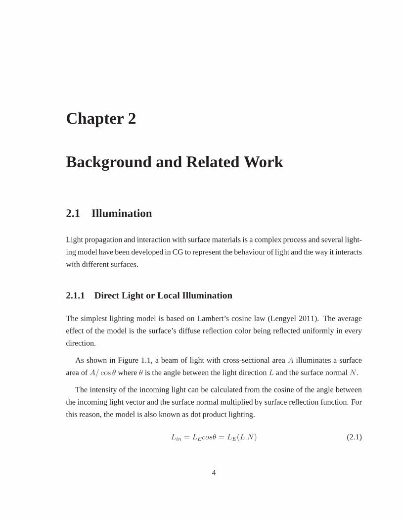
2.1.1 Direct Light or Local Illumination
The simplest lighting model is based on Lambert’s cosine law(Lengyel 2011). The average
effect of the model is the surface’s diffuse reflection colorbeing reflected uniformly in every
direction.
As shown in Figure 1.1, a beam of light with cross-sectional areaA illuminates a surface
area ofA/ cos θ whereθ is the angle between the light directionL and the surface normalN .
The intensity of the incoming light can be calculated from the cosine of the angle between
the incoming light vector and the surface normal multipliedby surface reflection function. For
this reason, the model is also known as dot product lighting.
Lin = LEcosθ = LE(L.N) (2.1)
4

where
Lin is the light intensity received by the surface
LE the light intensity emitted by the light source
θ the angle between the incoming light vector and the surface normal
L the normalized light vector of the incoming light
N the surface normal
Figure 2.1 The surface area illuminated by a beam of light increases as the angleθ between
the surface normal and direction to the light increases, decreasing the intensity of light per unit
area (Lengyel 2011).
2.1.2 Indirect Light or Global Illumination
Greater realism in image synthesis requires global illumination models which can account for
interreflection of light between surfaces (Cohen & Wallace 1993). The first global illumination
model introduced was with the recursive application of ray tracing to account for reflection,
refraction and shadows. It was recognized then, that the evaluation of global illumination
required determining the surface visibility in various direction from the point to be shaded.
Eventually more accurate physically based local reflectionmodels were developed using results
from the field of radiating heat transfer and illumination energy.
In contrast to earlier empirical techniques, the radiositymethod begins with an energy bal-
ance equation which is approximated and solved numerically. While ray tracing evaluates the
illumination equation for directions and locations determined by the view and the pixels of the
5
image, radiosity solves the illumination equation at locations distributed over the surfaces of
the environment.
Radiance and irradiance are basic optical quantities used to characterize emmission from
diffuse sources and reflection from diffuse surfaces respectively. A Lambertian surface reflects
light proportional to the incoming irradiance, so analysisof this physical system is equivalent
to a mathematical analysis of the relationship between incoming radiance and irradiance (Ra-
mamoorthi & Hanrahan 2001b). In other words, the radiosity method is an inverse rendering
approach that estimates the incoming light from the observations of a Lambertian surface.
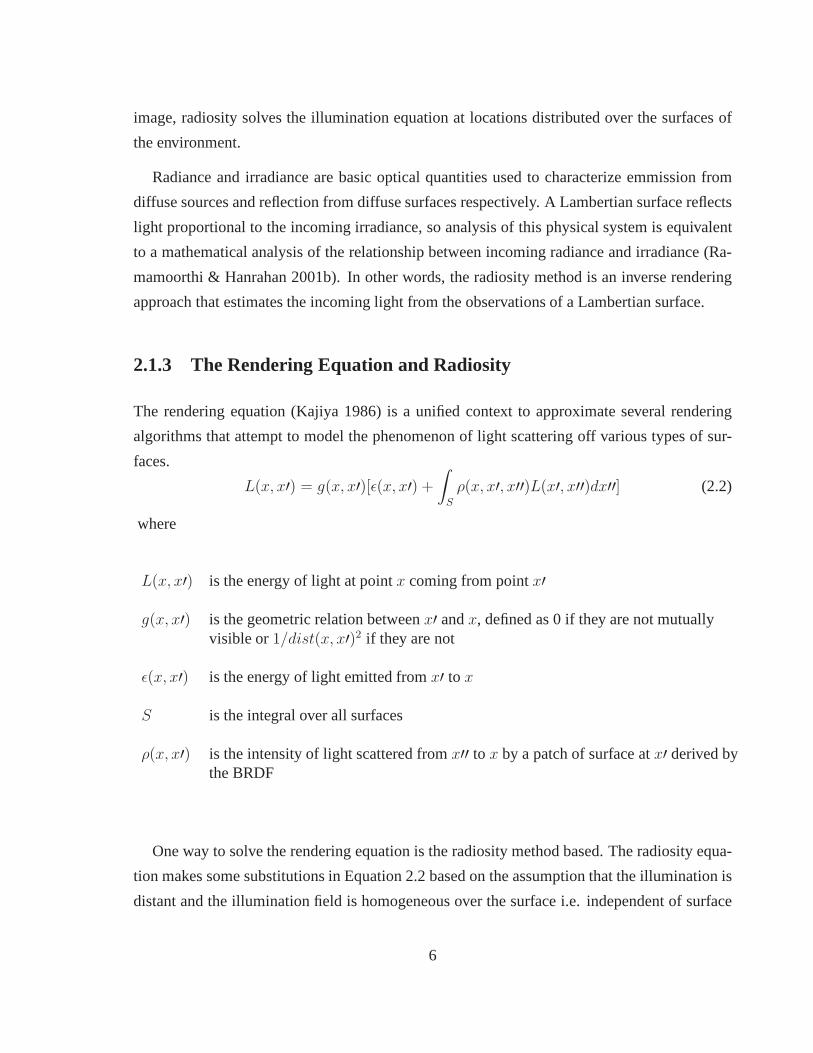
2.1.3 The Rendering Equation and Radiosity
The rendering equation (Kajiya 1986) is a unified context to approximate several rendering
algorithms that attempt to model the phenomenon of light scattering off various types of sur-
faces.
L(x, x′) = g(x, x′)[ǫ(x, x′) +
∫
S
ρ(x, x′, x′′)L(x′, x′′)dx′′] (2.2)
where
L(x, x′) is the energy of light at pointx coming from pointx′
g(x, x′) is the geometric relation betweenx′ andx, defined as 0 if they are not mutuallyvisible or1/dist(x, x′)2 if they are not
ǫ(x, x′) is the energy of light emitted fromx′ to x
S is the integral over all surfaces
ρ(x, x′) is the intensity of light scattered fromx′′ to x by a patch of surface atx′ derived bythe BRDF
One way to solve the rendering equation is the radiosity method based. The radiosity equa-
tion makes some substitutions in Equation 2.2 based on the assumption that the illumination is
distant and the illumination field is homogeneous over the surface i.e. independent of surface
6

positionx and depends only on global incident angle(θi, φi). This allows us to represent the il-
lumination field asL(θi, φi). Since the illumination field is distant we may also reparameterize
the surface by the surface normaln (Ramamoorthi & Hanrahan 2001b).
E(n) =
∫
Ω
′L(θi, φi)cosθi′dΩ′ (2.3)
where
E(n) is the irradiance independent of the surface positionx
L(θi, θi) is the radiance of the light field.
primes denote quantities in local coordinates
With an appropriate rotation on the lighting, we can convertit to the local coordinates(θi′, φi′)
L(θi, φi) = L(Rα,β,γ(θi′, φi′)) (2.4)
whereRα,β,γ is the rotation operator expressed in terms of standard Euler-angle representations.
Figure 2.2Diagram showing how the rotation corresponding toR(α, β, γ) transforms between
local (primed) and global (unprimed) coordinates (Ramamoorthi & Hanrahan 2001b).
7
Finally, we plug Equation (2.4) into Equation (2.3) to derive
E(α, β, γ) =
∫
Ω
′L(Rα,β,γ(θi′, φi′))A(θi′)dΩ′ (2.5)
where for convenience, we define a transfer functionA(θi′) = cos θi′
Ramamoorthi points out that this equation is essentially a convolution, although we have a
rotation operator rather than a translation.The irradiance can be viewed as a convolution of the
incident illuminationL and the transfer functionA = cos θi′. Different observations of the
irradianceE, at points on the object surface with different orientations, correspond to different
rotations of the transfer function, which can also be thought of as different rotations of the
incident light field.
This analogy of the radiosity model with convolution is whatwe will use to transform the
light field into Spherical Harmonics. We will deconvolve theirradiance to recover the inci-
dent illumination. The next chapter will deal Spherical Harmonic functions and their use for
lighting.
2.2 RenderMan
The first release of the RendeMan API was defined as a set of C functions which could be
called by modelling programs to pass instructions to a renderer. A modelling program makes
calls to the C API internally to create a RenderMan standard file. The RenderMan Interface
Byte (RIB) file format stream is the format that RenderMan compliant renderers read. RIB
files define the geometry and RenderMan distinguishes betwenthe shape of a geometry and its
surface detail (Stephenson 2007).
Each piece of geometry is bounded by a bounding box andsplit andbounded recursively
until the primitives reach a setbucket size. Thebucket sized polygons arediced into smaller
rectangularmicropolygons. Each of thesemicropolygons cover the same amount of screen
space.
The vertices of thesemicropolygons is what the shading engine runs on. After displacing
and shading, RenerMan determines which of themicropolygons are to beculled depending
8

on a visibility test and frustrum. The final image is calculated with a user-defined number of
samples. A number ofsamplesare fired to collect the color values. This is normally done on
a sub-pixel base to avoid aliasing. The user-defined reconstructionfilter then determines the
final colour from the transition between neighboring pixels(Upstill 1989).
9
Chapter 3
Spherical Harmonics
We have established in Section 2.1.3 the analogy of the radiosity method with convolutions.
Just as the Fourier basis is used to evaluate convolutions over the unit circle for one-dimensional
functions, spherical harmonics can do the same over the unitsphere for two-dimensional func-
tions (Sloan 2008).
3.1 Orthogonal basis functions
Similar to basis vectors that form a vector space, basis functions combine with other basis
functions to form afunction space. A function space defines a set of possible functions. For
example, the radiosity function is in the space ofL2 functions over some finite domainS (e.g.
the surfaces) Cohen & Wallace (1993)
Basis functions are small pieces of signal that can be scaledand combined to produce an
approximation to an original function. The process of working out how much of each basis
function to sum is called projection (Green 2003).
Figure 3.1 shows an example of a set of linear basis functions, giving us a piece-wise linear
appropriation to the input function. We can use many basis functions, but we are interested
here in a family of functions calledorthogonal polynomials.
10

Figure 3.1Approximation of a function using linear basis functions (Cohen & Wallace 1993).
11
Orthogonal polynomials exhibit an interesting property when the product of any two such
polynomials is integrated. The integral is a constant if they are the same and zero if they are
different.∫
1
−1
Fm(x)Fn(x)dx =
0 for, n 6= m
c for, n = m(3.1)
If the rule is made more rigorous such that integration must return either0 or 1, then this would
make a sub-family of functions called theorthonormal basis functions.
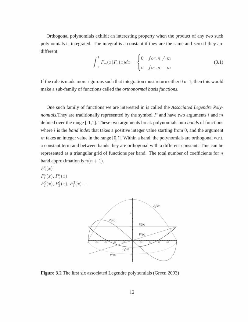
One such family of functions we are interested in is called the Associated Legendre Poly-
nomials.They are traditionally represented by the symbolP and have two argumentsl andm
defined over the range [-1,1]. These two arguments break polynomials intobands of functions
wherel is theband index that takes a positive integer value starting from0, and the argument
m takes an integer value in the range [0,l]. Within a band, the polynomials are orthogonal w.r.t.
a constant term and between bands they are orthogonal with a different constant. This can be
represented as a triangular grid of functions per band. The total number of coefficients forn
band approximation isn(n + 1).
P 00 (x)
P 01 (x), P 1
1 (x)
P 02 (x), P 1
2 (x), P 22 (x) ...
Figure 3.2The first six associated Legendre polynomials (Green 2003)
12

For an efficient computation of the Associated Legendre Polynomials, we use a set recur-
rence relations that generate the current polynomial from earlier results in the series (Green
2003).
This is the first identity to begin with as it takes no previousvalues
P mm = (−1)m(2m − 1)!!(1 − x2)m/2 (3.2)
The next equation is used to find a higher band polynomial.
P mm+1 = x(2m + 1)P m
m (3.3)
The third equation is the recursive calculation where we canfind thenth Legendre polynomial
using two previous bandsl − 1 andl − 2
(l − m)P ml = x(2l − 1)P m
l−1 − (l + m − 1)P ml−2 (3.4)
3.2 Spherical Harmonics
Spherical Harmonics define anorthonormal basis over the sphere,s.Using the standard param-
eterization
s = (x, y, z) = (sin θ cos φ, sin θ sin φ, cos θ) (3.5)
wheres are simply locations on the unit sphere. The basis functionsare defined as
Y ml (θ, φ) = Km
l eimφP|m|l (cos θ), l ∈ N,−l ≤ m ≤ l (3.6)
whereP mm are the associated Legendre polynomials andKm
l are the normalization constants
Kml =
√(2l + 1)(l− | m |)!
4π(l+ | m |)! (3.7)
13

The above definition is for the complex form (most commonly used in the non-graphics litera-
ture), a real valued basis is given the transformation (Sloan 2008)
yml = x =
√2Re(Y m
l ) m > 0√
2Im(Y ml ) m < 0
Y 0l m = 0
=
√2Km
l cos mφP ml (cos θ) m > 0
√2Km
l sin | m | φP|m|l (cos θ) m < 0
K0l P 0
l (cos θ) m = 0
(3.8)
Figure 3.3 The first 5 SH bands plotted as unsigned spherical functions by distance from the
origin and by colour on a unit sphere. Green (light ray) are positive values and red (dark gray)
are negative. (Green 2003).
3.3 Spherical Harmonic Projection
Projecting a function into basis functions is in effect working out how much of the function is
like the basis function. To calculate a single a single coefficient for a specific band we integrate
the product of the functionf and the SH functiony.
14

Since the SH Basis is orthonormal the projectin of a scalar functionf defined overs is done
by simply integrating the function you want to project,f(s), against the basis functions
fml =
∫f(s)ym
l (s)ds (3.9)
These coefficients can be used to reconstruct an approximation of the functionf
f(s) =
n∑
l=0
l∑
m=−l
fml ym
l (s) (3.10)
which is increasingly accurate as the number of bandsn increases.Projection ton-th order
generatesn2 coefficients. For convenience a single index for both the projection coefficients
and the basis coefficients is used.
f(s) =
n2∑
i=0
fiyi(s) (3.11)
wherei = l(l + 1) + m.
This formulation makes it clear that approximating the function at directions is simply a dot
product betweenn2 coefficient vactorfi and the vector of evaluated basis functionsyi(s) (Sloan
2008)
3.4 Properties of SH functions
Orthonormality
One of the properties of SH functions that makes them desirable as basis functions is that they
are not just orthogonal but also orthonormal. This means if we integrateyiyj for any pair ofi
andj, the calculation will return 1 ifi = j and 0 ifi 6= j (Refer to Equation(3.1)). This makes
it easy to recontruct the approximation function.
Rotational invariance
SH functions are rotationally invariant.This means if a function g is a rotated copy of function
15
f , then after SH projectiong(s) = f(R(s)). This rotational invariance is similar to the transla-
tional invariance in the Fourier transform. This means thatthere would be no aliasing artifacts
or fluctuation in the light sources when CG scenes have animated lights and models.
Efficient Integration
In the context of lighting, the incoming illumination wouldhave to be multiplied by the surface
reflectance to get the resulting reflected light.This integration is done over the entire incoming
sphere∫
SL(s)t(s)ds
whereL is the incoming light andt is the surface reflectance. If both these functions are pro-
jected into SH coefficients then orthogonality reduces the integral of the functions’ products to
just the dot product of their coefficients.
∫
S
L(s)t(s)ds =
n2∑
i=0
Liti (3.12)
For further reading, the articles by (Sloan 2008) and (Green2003) provide a deeper insight
into spherical harmonic lighting.
16
Chapter 4
Implementation
The preceding chapters described general CG principles in the context of lighting and the
solution spherical harmonics can provide to solve the problem more efficiently. This chapter
deals with the actual implementation of it first as a test bench in C++ to verify the computations
and then goes on to describe the shaders that have been implemented in RenderMan.
4.1 C++ Test Bench
Based on the sample codes in Green’s paper a simple computational prototype was imple-
mented in C++. The paper provides a sample light equation andthe SH coefficients for it.
Once the basis functions were calculated, this known light equation was projected and the
values were compared.
Implementing this basic computation gave an idea of the subroutines that the program would
need to be broken into to provide extended functionality to RenderMan.
4.2 Dynamic Shared Object
It is possible to write arbitrary functions in RenderMan Shading Language (RSL) but it has
certain limitations. The RSL compiler inlines a function every time the function is called and
17

thus the function code is not shared among its invocations. It is not possible for different
shaders to call the same function without additional redundant definition.
C++ functions that are linked as plugins to RSL can overcome this limitation. Once the C++
function is compiled and linked to RSL as a plugin, the resulting object code from it is shared
among all its invocation. The C++ function can call functions from the standard C/C++ library
or even third party libraries. Another advantage is that theC++ function is not limited to RSL
datatypes unlike RSL functions. One can create complex datastructures or read external files
or do anything that one might do in a compiled program (Pixar 2006).
Plugins do have some limitations that should be borne in mind. Plugins have access to only
the information passed to them as parameters and they cannotcall any RSL built-in functions.
They do not support Objective C and have no knowledge of the topology. The new interface
supersedes the oldershadeop which is something to be aware of as a developer (Pixar 2006).
The C++ file includes the header,RslPlugin.h which contains the class definitions and
macros that will be used. RSL requires plugins to use C-stylelinkage for the plugin loading
system. To ensure this,extern "C" was used around tables and functions.
The RslPublicFunctions Table describes two functions contained in the plugin.
shadeop_sh(float, float, float, float)
shOcclusion(float[], vector)
The functionshadeop_sh calculates the SH basis functions. It takes as parameters the
bandl, m in the range [0,l] and the spherical coordinatestheta, phi. The function is
called for every shading point and the shader is given back the basis coefficients for that point.
The functionshOcclusion reads in the array of basis coefficients from a shading point
and projects the light vector passed to it as a parameter. From the directional visibility deter-
mined by the basis coefficients and given the light vector thefunction calculates how illumi-
nated or unoccluded that point is.
The following sections will describe how these functions are used in the shader.
18

4.3 RenderMan Workflow
Given the geometry and the lights in a scene RenderMan will configure the lights to make them
capable of Spherical Harmonic Lighting in three passes. Theapproach is to read in the RIB
file, generate a point cloud of it and thenbake data into the point cloud file. The SH-configured
light will then read in the information in the point cloud fileto determine the light and shade
of the point.
A point cloud is just a cloud of points in 3d space that contains one or more channels of data
(lighting, occlusion, area, etc) at each point. They are theimmediate precursor to abrickmap,
which is a useful structure for caching data as a3d texture.
RenderMan generates point clouds very efficiently because of the way the REYES algo-
rithm dices geometry. For every micropolygon, it can simplywrite a point to the point cloud
(or optionally a point for each corner of the micropolygon),that contains the point’s location
in space, its normal, and any data that the user specifies (Pixar 2013).
Figure 4.1Shows an example of point cloud data (Pixar 2013)
4.4 simpleBake.sl
The first shader to be invoked is thesimpleBake. It is an extended version of the bake˙areas
surface shader (Pixar 2013). It generates a point cloud of the scene geometry that the subse-
19
quent shaders can bake data into. The shader writes out the standard shader output variable
float _area to the point cloud.
Figure 4.2Shows a point cloud snapshot of a simple test scene
4.5 shBasis.sl
This shader is at the heart of the pipeline. The shader reads in the previous point cloud file and
for eachmicropolygon it generates the basis coefficients. It is a time consuming pre-process as
we will see in the statics shown in the next chapter.
Using thegather function, the shader collects visibility information. Foreachmicropoly-
gon a number of rays are cast across the hemisphere. The rays thatintersect are not of interest
to us. The ones that are missed are the visiblemicropolygons. These missed ray directions
accessed from the output variable"ray:direction", are converted into spherical coordi-
nates and stored in an array.
20

The shader then computes the coefficients by looping coefficient times (i.e.(l+1)∗ (l +1))
over the samples and calling theshadeop_sh plugin function with the appropriate band value
l, m, and the array the spherical coordinates as parameters. Thecoefficents are then multipied
by a weighting factor4π/samples i.e the area of a unit sphere divided by the number of sam-
ples.
The coefficients are then baked into the point cloud as channels using thebake3d function.
Figure 4.3Shows coeff ˙00 channel in the point cloud. All the coefficients baked in the point
cloud and store directional visibility
4.6 shProjection.sl
The projection shader reads in the previous point cloud withthe basis coefficients and projects
the light vector into it. The shader generates another pointcloud file with the channels
"unoccluded" and"lightCol". The"unoccluded" channel represents how illumi-
nated the surface is at that point and"lightCol" is the colour of incoming light at that
21

point.
Theilluminance statement integrates the incoming light over a cone angle. Inside the
illuminance block, we can access the light colour and the light directionfrom the prede-
fined variablesCl andL respectively.
The basis point cloud is read inside theilluminance block and the coefficients are stored
in an array. This array and the light vector are passed as parameters to theshOcclusion plu-
gin function. TheshOcclusion function converts the light vector into spherical coordinates
and projects it into SH space. The integration then is reduced to a single dot product over the
SH coefficients (Refer to Section(3.4)).
The result of the integration is a single scalar value that isbaked into the point cloud in the
"unoccluded" channel. The colour of the light from that direction is also baked into the
"lightCol" channel. This is done so that we can call the same shader to project monochro-
matic as well as coloured lights. Projecting an environmentlight then becomes just a special
case of coloured light.
Figure 4.4Shows the unoccluded channel in the point cloud after the projection of the light.]
22
4.7 shLight.sl
The shlight is a light shader that can now use the projection point cloud to create shadows.
There is an intermediate step to convert the point clouds to brickmaps for the sake of effi-
ciency but it is not a necessity. Apart from efficiency, brickmaps also provide certain filtering
parameters that can be used to tweak the output.
The light shaders used for demonstration are extensions of the standard RenderMan lights.
The illuminate statement casts light into the scene in different directions depending on
the parameters specified. But unlike the standard lights that would usually call theshadow
function or therayinfo function to compute shadows, the shLight can just use themix
function to blend the light and shadow colours using the"unoccluded" channel as the
blend value.
4.7.1 Types of Light
Once the pre-process is done it is fairly simple to supply thelight shader the brickmap to use
for shadowing using thetexture3d function. One of the benefits of reading the SH data
using thetexture3d function is that it can be used as just a texture or surface color. This
would make the data available in a surface shader which is a typical production practice with
ambient-occlusion passes and light passes.
Shown below are renders of a simple scene using the differentshLight shaders that have
been developed. The same projection has also been used as a surface shader to demonstrate the
results. The decision between surface or light shader is largely a matter of choice and workflow
on the part of the user.
23

Figure 4.5Shows a simple scene with the different types of light that have been implemented
across rows. Along the columns are the different shaders that call in the baked brickmaps
24
Chapter 5
Results and Analysis
The PRMan shaders described in the previous chapter will be tested against standard methods
in this chapter. The tests are conducted to analyze the efficiency of the pre-computed SH
method and the quality of the result.
5.1 Efficiency
The simple scene used earlier for light demonstrations has been used as an example in this
section. Similar differences in performance have been seenwith the other examples that will
be illustrated in this chapter.
The scene was rendered with a raytraced ambient occlusion surface shader and compared
with the render time of the SH directional occlusion also applied as a shader to the surface.
The following graph compares the performace of the two methods. The scene contains 210
micropolygons and was rendered with 256 samples in both cases.
The SH data is computed for 16 coefficients i.el = 3, which is considered a fairly sufficient
approximation for production lighting. The precomputation time for the SH method is 1260
seconds and then it can reuse the baked data to render a frame in about 2 seconds. The standard
ray-tracing method takes about 24 seconds per frame.
25
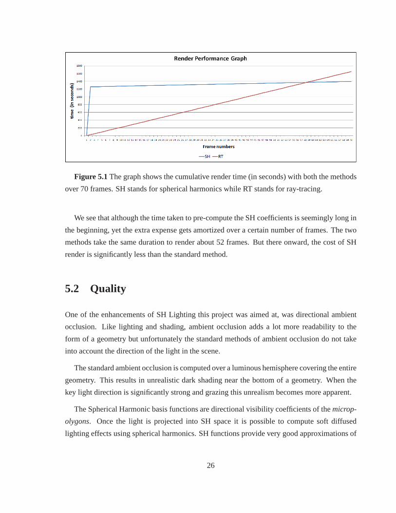
Figure 5.1The graph shows the cumulative render time (in seconds) withboth the methods
over 70 frames. SH stands for spherical harmonics while RT stands for ray-tracing.
We see that although the time taken to pre-compute the SH coefficients is seemingly long in
the beginning, yet the extra expense gets amortized over a certain number of frames. The two
methods take the same duration to render about 52 frames. Butthere onward, the cost of SH
render is significantly less than the standard method.
5.2 Quality
One of the enhancements of SH Lighting this project was aimedat, was directional ambient
occlusion. Like lighting and shading, ambient occlusion adds a lot more readability to the
form of a geometry but unfortunately the standard methods ofambient occlusion do not take
into account the direction of the light in the scene.
The standard ambient occlusion is computed over a luminous hemisphere covering the entire
geometry. This results in unrealistic dark shading near thebottom of a geometry. When the
key light direction is significantly strong and grazing thisunrealism becomes more apparent.
The Spherical Harmonic basis functions are directional visibility coefficients of themicrop-
olygons. Once the light is projected into SH space it is possible to compute soft diffused
lighting effects using spherical harmonics. SH functions provide very good approximations of
26
low frequency lights and are thus preferred for rendering ambient occlusion and environment
lights.
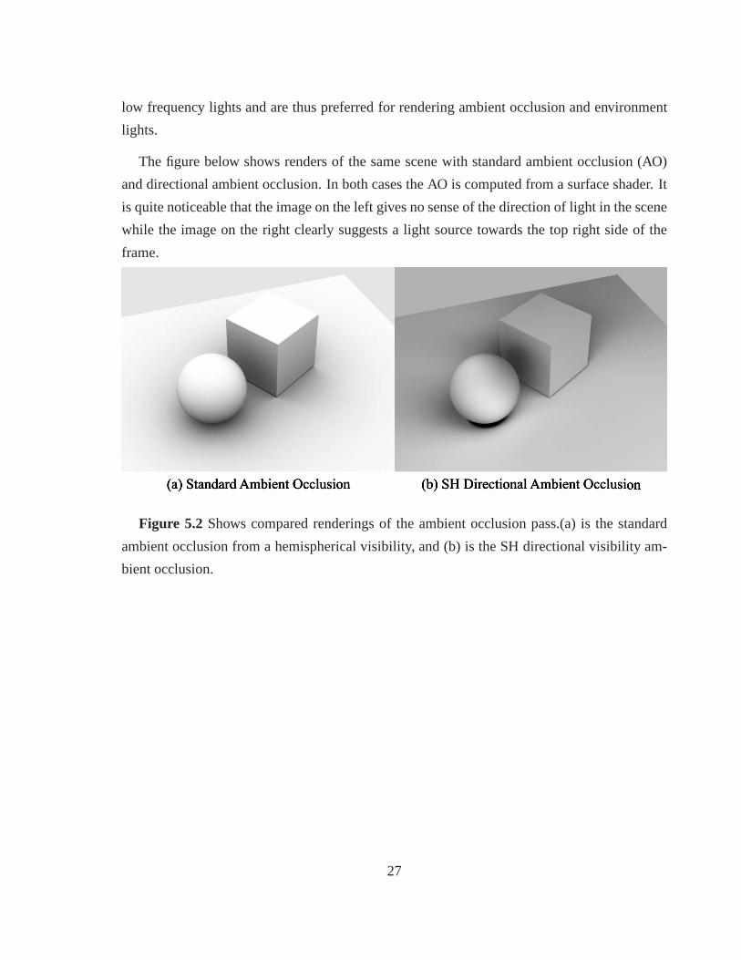
The figure below shows renders of the same scene with standardambient occlusion (AO)
and directional ambient occlusion. In both cases the AO is computed from a surface shader. It
is quite noticeable that the image on the left gives no sense of the direction of light in the scene
while the image on the right clearly suggests a light source towards the top right side of the
frame.
Figure 5.2 Shows compared renderings of the ambient occlusion pass.(a) is the standard
ambient occlusion from a hemispherical visibility, and (b)is the SH directional visibility am-
bient occlusion.
27
5.3 Examples and Comparisons
This section will use SH lighting on more complex scenes and lighting scenarios to demonstrate
the robustness of the shaders developed and stress on the believability of the images rendered
using SH lighting.
5.3.1 SH Direct
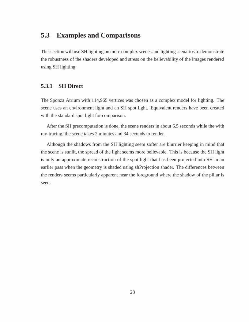
The Sponza Atrium with 114,965 vertices was chosen as a complex model for lighting. The
scene uses an environment light and an SH spot light. Equivalent renders have been created
with the standard spot light for comparison.
After the SH precomputation is done, the scene renders in about 6.5 seconds while the with
ray-tracing, the scene takes 2 minutes and 34 seconds to render.
Although the shadows from the SH lighting seem softer are blurrier keeping in mind that
the scene is sunlit, the spread of the light seems more believable. This is because the SH light
is only an approximate reconstruction of the spot light thathas been projected into SH in an
earlier pass when the geometry is shaded using shProjectionshader. The differences between
the renders seems particularly apparent near the foreground where the shadow of the pillar is
seen.
28
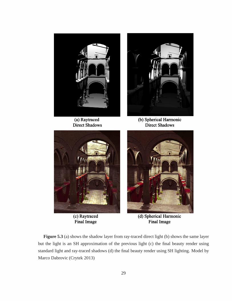
Figure 5.3(a) shows the shadow layer from ray-traced direct light (b) shows the same layer
but the light is an SH approximation of the previous light (c)the final beauty render using
standard light and ray-traced shadows (d) the final beauty render using SH lighting. Model by
Marco Dabrovic (Crytek 2013)
29

5.3.2 SH Indirect
The next example uses SH for indirect lighting. This dressing table image was chosen as a
reference because it had a soft diffuse lighting. The stool in the image was replaced with a CG
one and the lighting was matched as an exercise to see how SH lighting could integrate better
with the image.
We can see two significant directions of light in the image. Using the directional ambient
occlusion shader, a separate occlusion pass was rendered for both the lights. The results were
combined to produce the final image.
The same CG setup and lighting was used to create a comparative image using standard
ambient occlusion. The environment light in both cases is the same.
Shown below are the actual photograph used as reference, theCG setup and the two dif-
ferent occlusion renders. In the standard occlusion image the stool looks as if it were lit by
a diffuse light from top.The creases and crevices in the carving on the leg of the stool seem
unusually dark as they are occluded from the uniform luminous hemisphere of light. The SH
occlusion on the other hand seems more believable when compared to the standard occlusion
as the directional occlusion is computed from the particular directions of the two lights used to
illuminate the scene.
30
Figure 5.4 (a) Shows the original photograph (NEST Furniture 2013) (b)shows the CG
setup (c) is the final image with standard ambient occlusion (d) is the final image with direc-
tional ambient occlusion
31

Figure 5.5Shows the raw ambient occlusion renders in the first column and their respective
close-ups in the second column. The third column shows the render statistics. (Render time is
32

in hh:mm:ss)
33
Chapter 6
Conclusion
6.1 Summary
A set of shaders have been presented that can extend the functionality of RenderMan to perform
spherical harmonic lighting and all the necessary precomputations. This has been achieved by
writing an RSL Plugin for RenderMan that is compiled as a Dynamic Shared Object(DSO).
A good part of the project has been dedicated to understanding the theoretical concepts
behind spherical harmonics. General CG principles for lighting and rendering have also been
discussed.
The efficiency of the results have been demonstrated throughcomputational times and the
quality of the renders, through the use of examples that spanacross different lighting condi-
tions.
6.2 Discussion
The implementation discussed in this thesis bakes point clouds from the camera view. If the
bake happened over a larger area from an orthographic top camera, then the data would be
more useful.
34
Only a limited set of lights have currently been implementedwhich is a bit restrictive when
trying to light a scene believably. A few more types of light implementations are needed to
make this a complete set of SH lights.
6.3 Future work
The shaders are currently not integrated well into a production pipeline. They could be inter-
faced neatly with RenderMan for Maya and made available to the user like a pass, much like
the standard globalillumin pass. The SH shaders can be extended to be used with lightshaders
from stdrsl. Getting these SH shaders to work with plausibleshaders would be an important
area of work.
This implementation does not calculate caustics or color bleeding. It would be beneficial to
incorporate such light effects. Subsurface scattering is another effect that is suitable for being
projected into spherical harmonics and hence another area for venturing.
On the lines of PantaRay’s implementation, the calculations handled by the plugin can be
outsourced to the Graphics Processing Unit to further enhance efficiency.
35
Bibliography
M. F. Cohen & J. R. Wallace (1993).Radiosity and Realistic Image Synthesis. Academic Press
Professional, USA.
Crytek (2013). ‘CryENGINE’. Available from: http://www.crytek.com/cryengine/cryengine3/downloads
[Accessed 15.08.2013].
R. Green (2003). ‘Spherical Harmonic Lighting:The Gritty Details’. Archives of the Game
Developers Conference .
J. T. Kajiya (1986). ‘The rendering equation’. InProceedings of the 13th annual conference on
Computer graphics and interactive techniques, SIGGRAPH ’86, pp. 143–150, New York,
NY, USA. ACM.
E. Lengyel (2011).Mathematics for 3D Game Programming and Computer Graphics. Course
Technology / Cengage Learning, USA.
NEST Furniture (2013). ‘Nest Designed for Kids’. Availablefrom:
http://www.nestdesigns.co.za/product/all-bedroom/darcy-dressing-table-stool-set-white/
[Accessed 15.08.2013].
J. Pantaleoni, et al. (2010). ‘PantaRay: fast ray-traced occlusion caching of massive scenes’.
vol. 29, pp. 37:1–37:10, New York, NY, USA. ACM.
Pixar (2006). ‘SIMD RenderMan Shading Language Plugins’. Available from:
http://webstaff.itn.liu.se/stegu/TNM022-2006/Pixar ˙RPS ˙13.0 ˙docs/prman ˙technical ˙ren-
dering/AppNotes/ [Accessed 15.08.2013].
Pixar (2013). ‘Pixar RenderMan’. Available from:
http://renderman.pixar.com/view/renderman [Accessed 15.08.2013].
36
R. Ramamoorthi & P. Hanrahan (2001a). ‘An efficient representation for irradiance environ-
ment maps’. InProceedings of the 28th annual conference on Computer graphics and inter-
active techniques, SIGGRAPH ’01, pp. 497–500, New York, NY, USA. ACM.
R. Ramamoorthi & P. Hanrahan (2001b). ‘On the relationship between radiance and irradiance:
determining the illumination from images of a convex Lambertian object’. J. Opt. Soc. Am.
A 18(10):2448–2459.
P.-P. Sloan (2008). ‘Stupid Spherical Harmonics (SH) Tricks’. Archives of the Game Develop-
ers Conference .
I. Stephenson (2007).Essential RenderMan. Springer-Verlag, London.
S. Upstill (1989). RenderMan Companion: A programmer’s Guide to Realistic Computer
Graphics. Addison-Wesley Longman Publishing Co., USA.
37
Recommended