Spatio-temporal modelling for airpollution

Sujit SahuSouthampton Statistical Sciences Research Institute,

University of Southampton

SAMSI, March 2013

Collaborators: Lee, Mitchell, Rushworth (Glasgow)Mukhopadhay, Bakar, Bass, Yip (PhD Students) and theUK Met Office.

1 A rigorous statistical framework for estimating thelong-term health effects of air pollution

2 Forecasting next day ozone levels in the eastern US

Spatio-temporal modelling for airpollution

Sujit SahuSouthampton Statistical Sciences Research Institute,

University of Southampton

SAMSI, March 2013

Collaborators: Lee, Mitchell, Rushworth (Glasgow)Mukhopadhay, Bakar, Bass, Yip (PhD Students) and theUK Met Office.

1 A rigorous statistical framework for estimating thelong-term health effects of air pollution

2 Forecasting next day ozone levels in the eastern US

Motivation

Air pollution has many detrimental effects to humanhealth: primarily respiratory, lung function, coughing,throat irritation, congestion, bronchitis, asthma.

According to the website of the Department forEnvironment Food and Rural Affairs (DEFRA):

“In 2008 air pollution in the form of anthropogenicparticulate matter (PM) alone was estimated toreduce average life expectancy in the UK by aroundsix months.

Thereby imposing an estimated equivalent healthcost of 19 billion GBP in 2008.”

Traffic pollution kills 5,000 a year in UK, says study: BBCNews, April 17, 2012.

Sujit Sahu 2

Three main aims of our project

A Development of a model that provides an accuraterepresentation of the spatio-temporal structure insmall-area health data.

B Development of a model that produces estimates andmeasures of uncertainty in the levels of overall airpollution at relevant spatial and temporal resolutions(as required to align with the health data).

C Development of a single integrated framework forcombining the health and pollution models describedin A and B, thus allowing the chronic effects of airpollution to be estimated.

Sujit Sahu 3

Specific Research Objectives (SRO)

(i) To develop a Bayesian spatio-temporal Markovrandom field (MRF) model that can representlocalised spatial structure and identify boundaries inhealth data.

(ii) To apply the model to real and simulated data sets, toquantify the impact that mis-specifying the spatialstructure of the unmeasured confounders has on theestimated pollution-health relationship.

Sujit Sahu 4

Specific Research Objectives...

(iii) To develop a Bayesian multiple pollutant space-timegeostatistical model that can predict levels of overallpollution at unmonitored locations with theirassociated uncertainties.

(iv) To validate the model in SRO (iii) using air pollutiondata in study regions.

(v) To combine the MRF model in (i) and geostatisticalmodel (iii) to estimate the effects of air pollution onhuman health in three case studies: London,Southampton and Glasgow.

Sujit Sahu 5

Specific Research Objectives...

(vi) To study the effect of future climate on health and airpollution, by using UK specific regional climate modelprojections to 2050 that will be used in the integratedhealth-pollution model.

(vii) To develop a user-friendly software package enablingothers to implement the methods that we develop.

Sujit Sahu 6

Health outcome model

Let Yt (Ai) and Et(Ai) denote the observed andexpected numbers of health events that occur in arealunit Ai (i = 1, . . . , n) and time period t (t = 1, . . . ,T ),such as respiratory admissions to hospital.

The overall risk Rt(Ai) is modelled by covariatesx′t(Ai) and a random effect φt(Ai).

Yt(Ai) ∼ Poisson(Et(Ai)Rt(Ai)),log(Rt(Ai)) = x′t(Ai)β+ φt(Ai).

Sujit Sahu 7

Modelling the random effects

Denote the random effects by φ = (φ1, . . . ,φT ), whereφt = (φt(A1), . . . , φt(An)),we propose a class of MRF priors which decomposef (φ1, . . . ,φT ) :

p∏

t=1

N(φt |0, τ2t Q−1

t )

andT∏

t=p+1

N(φt |F1tφt−1 + · · ·+ Fptφt−p, τ2t Q−1

t ).

Fjt are the temporal transition matrices,p denotes the lag of the temporal correlation and istypically chosen to be one or two.

Sujit Sahu 8

Modelling the random effects...

Temporal correlation induced via the mean structure.

Spatial correlation is induced via the variancestructure.

The latter is parameterised by the precision matrixQt , whose jk th element controls the spatialcorrelation structure between φt(Aj) and φt(Ak ).

Qt constant is a possibility.

Sujit Sahu 9

Air pollution model

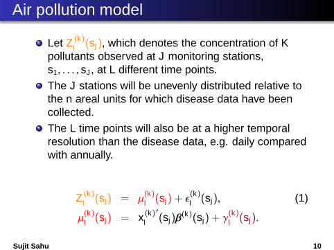
Let Z (k)

l (sj), which denotes the concentration of Kpollutants observed at J monitoring stations,s1, . . . , sJ , at L different time points.

The J stations will be unevenly distributed relative tothe n areal units for which disease data have beencollected.

The L time points will also be at a higher temporalresolution than the disease data, e.g. daily comparedwith annually.

Z (k)

l (sj) = µ(k)

l (sj) + ǫ(k)

l (sj), (1)

µ(k)

l (sj) = x (k)

l

′

(sj)β(k)(sj) + γ

(k)

l (sj).

Sujit Sahu 10

Air pollution model...

The error term ǫ(k)

l (sj) is assumed to be a pollutantspecific white noise process.

The true concentration of pollution will be modelledby a combination of covariates x (k)

l (sj),

and a spatio-temporal processγl(sj) = (γ

(1)

l (sj), . . . , γ(K )

l (sj)).

We propose representing the space-time processγl(sj) with the linear model of co-regionalisation,γl(sj) = Dlηl(sj), which uses the correlations betweenthe pollutants to improve the fit of the model.

Sujit Sahu 11

Estimating overall air quality index (AQI)

θl(sj) =1K

K∑

k=1

µ(k)

l (sj) − µ(k)

sd(µ(k)),

where µ(k) and sd(µ(k)) are the sample mean andstandard deviation of µ(k)

l (sj).

A Bayesian approach will enable us to produceposterior distributions for θl(sj), which in turn allowsus to quantify the uncertainty in the AQI.

Sujit Sahu 12

The link model...

θt(A) = |A|−1∫

Aθt(s)ds, (2)

where |A| denotes the area of block A

log(Rt(Ai)) = β0θt−1(Ai) + x ′t (Ai)β+ φt(Ai). (3)

Here β0 is the effects of air pollution on health.The AQI is lagged by one year compared with thehealth data to ensure that the ‘exposure’ occursbefore the response.A Measurement error model links θt(Ai) and θl(sj) by

θt(Ai) ∼ N(θt(Ai), σ2θ),

where θt(Ai) is the average of all θl(sj) where sj is withinareal unit i and l is within the aggregate time t .

Sujit Sahu 13

Discussion

The models are under currently construction: twopost-docs: Mukhopadhyay (Southampton) andRushworth (Glasgow).

Software packages implementing the models will bedeveloped.

Three year EPSRC, like NSF, project worth 635K.Launch meeting in Southampton on April 15, 2013.

We would like to learn more from data from India.

We need pollution and health data.

A post-doc/PhD student, preferably from India, whocan harass the government for releasing the data!

A collaborator, like many Indian colleagues, as well.

Sujit Sahu 14

2: Forecasting next day ozone levels in theeastern United States

1 Three Gaussian process models.2 Forecast calibration with a small example.3 Illustration with a large data set.4 Discussion.

Sujit Sahu 15

Preliminaries in modelling

Apply transformation to stabilize variance and toencourage symmetry etc.

We use the square root, but it is possible to use thelog.

Observed data = Zl(s, t), s = (long, lat)′, at n sites.

Denote time by two indices: t for hours (days) within lfor days (years).

Data are observed at n sites s1, . . . , sn.

As a covariate in a downscaler model (Sahu et al2009, Berrocal et al 2010) we use the grid CMAQ(computer model) output, x l(s, t).We can use other covariates, e.g. temperature,windspeed and relative humidity, but those do notremain significant after including CMAQ output.

Sujit Sahu 16

Model 1: Gaussian Process (GP)

Measurement error model:

Zl(s, t) = Ol(s, t) + ǫl(s, t), ǫl(s, t) ∼ N(0, σ2ǫ ).

Ol(s, t) = true value, underlying space-time process.

ǫl(s, t) are independent.

σ2ǫ is called the ‘nugget’ effect.

Model for true ozone

Ol(s, t) = x l(s, t)′β+ ηl(s, t)

x l(s, t)′β: adjustment for local meteorology and/orother covariates, e.g. CMAQ output.

ηl(s, t): space-time intercept, assumed to beindependent in time.

Assume ηlt ∼ N(0, Ση), Ση = σ2η× Matern correlation.

Sujit Sahu 17

Model 2: AR models

Measurement error model:

Zl(s, t) = Ol(s, t) + ǫl(s, t), ǫl(s, t) ∼ N(0, σ2ǫ ).

Details as before.

Model for true ozone

Ol(s, t) = ρOl(s, t − 1) + x l(s, t)′β+ ηl(s, t)

ρOl(s, t − 1): auto-regressive.

x l(s, t)′β: adjustment for local meteorology and/orother covariates, e.g. CMAQ output.

ηl(s, t): space-time intercept, independent in time.

Assume ηlt ∼ N(0, Ση), Ση = σ2η× Matern correlation.

Need an initial condition when t = 1. Details omitted.Sujit Sahu 18

Model 3: GPP approximations: Banerjee et al2008

Ideally, in addition to the nugget effect, would like tofit:

Ol(s i , t) = x l(s i , t)′β+ ηl(s i , t). (4)

The problem is that then we will have nrT space-timerandom variables ηl(s i , t), the same number as data.GPP approximations, reduce this number byconsidering a smaller number, m << n, of knotlocations, denoted by s∗1, . . . , s

∗m.

Consider a spatial Gaussian processη∗lt = (ηl(s∗1, t), . . . , ηl(s∗m, t)) at the knots.Based on the above process, obtain a kriged valueηl(s i , t) at each of the observation sites.Now, instead of (4), we fit the model:

Ol(s i , t) = x l(s i , t)′β+ ηl(s i , t).Sujit Sahu 19

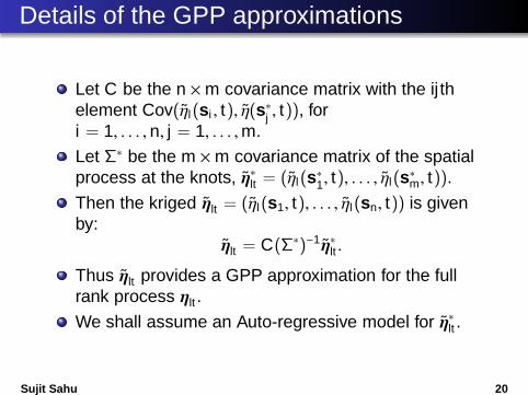
Details of the GPP approximations

Let C be the n ×m covariance matrix with the ij thelement Cov(ηl(s i , t), η(s∗j , t)), fori = 1, . . . , n, j = 1, . . . ,m.

Let Σ∗ be the m ×m covariance matrix of the spatialprocess at the knots, η∗lt = (ηl(s∗1, t), . . . , ηl(s∗m, t)).Then the kriged ηlt = (ηl(s1, t), . . . , ηl(sn, t)) is givenby:

ηlt = C(Σ∗)−1η∗lt .

Thus ηlt provides a GPP approximation for the fullrank process ηlt .

We shall assume an Auto-regressive model for η∗lt .

Sujit Sahu 20

Dynamic η∗lt .

Auto-regressive model

η∗lt = ρη∗lt−1 + ωlt

ρ is the auto-regressive parameter.

ωlt ∼ N(0,Σ∗) independently in time l and t .

CommentsThe spatial knot locations do not change in time.

Hence, this can handle cross sectional data wheredifferent locations are sampled at each time point.

It is possible to consider knots in time as well.

Knots do not need to be regularly spaced.

A sensitivity study may be conducted for the knotselections, Sahu and Bakar (2012).

Sujit Sahu 21

Setting up the GPP approximations

Figure: 691 ozone monitoring sites in the eastern US. The12 × 12 knot locations are superimposed.

Sujit Sahu 22

Forecast calibration

Bayesian forecasts are given by posterior predictivedistributions of Yl(s0, t) at any location s0 and timedenoted by two indices l and t .

Simplify notation Yl(s0, t) to Yi where i denotes theparticular combination value of s0, l and t .

Assume that the forecast at i has the cumulativedistribution function (CDF), Fi(y).

The calibration problem is to compare Fi(y) withGi(y) where Gi(y) is the true unknown forecast CDF.

Fi(y) is not available in closed form, but we haveMCMC samples y (j)

i , j = 1, . . . , J for a large J.

We shall try to assess how close is F to G on thebasis of m validation observations yi , i = 1, . . . ,m andthe MCMC samples y (j)

i .Sujit Sahu 23

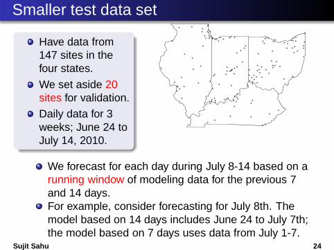
Smaller test data set

Have data from147 sites in thefour states.

We set aside 20sites for validation.

Daily data for 3weeks; June 24 toJuly 14, 2010.

*

*

*

*

*

*

*

****

***

**

*

*

*

*

****

**

*

* *

**

*

*

*

*

** *

***

*

*

**

*

*

**

*

****

*

*

**

*

*

*

**

*

*

**

*

*

*

**

*

* *

*

**

*

*

*

**

*

**

**

*

*

*

*

*

**

**

*

*

*

**

**

*

*

*

*

*

* *

***

* *

*

*

*

*

*

*

*

*

*

*

*

**

*

*

**

**

*

*

We forecast for each day during July 8-14 based on arunning window of modeling data for the previous 7and 14 days.For example, consider forecasting for July 8th. Themodel based on 14 days includes June 24 to July 7th;the model based on 7 days uses data from July 1-7.

Sujit Sahu 24

Hit and false alarm rates

Let y0 be a given threshold value (usually a highregulatory criterion value).

Hit(y0) =1m

m∑

i=1

{

1 (yi > y0 & yi > y0) + 1 (yi < y0 & yi < y0)}

False alarm(y0) =1m

m∑

i=1

1(yi < y0 & yi > y0).

Model 14 days dataOzone levels Model False alarm Hit rate

65 ppbGP 0.92 91.67AR 1.83 92.50GPP 2.75 91.67

75 ppbGP 0.0 95.83AR 0.0 95.83GPP 0.0 97.50

Table: False alarm and hit rates for ozone threshold values of65 and 75 for the four states data set.

Sujit Sahu 25

Continuous ranked probability score

Let Y and Y ′ independently follow F . Define

crps(F , y) = EF |Y − y | −12

EF |Y − Y ′|

CRPS =1m

m∑

i=1

crps(Fi , yi) for hold-outs y1, . . . , ym.

Values from modeling 7 days dataModels 7/8 7/9 7/10 7/11 7/12 7/13 7/14 7/(8-14)GP 6.12 10.22 5.04 5.05 4.78 5.70 6.95 6.27AR 6.19 10.12 4.95 5.31 4.85 4.38 4.31 5.73GPP 4.95 10.02 4.89 5.33 4.87 4.33 4.13 5.52

Values from modeling 14 days dataGP 6.14 9.82 5.33 5.42 5.21 5.64 6.29 6.27AR 5.91 9.83 4.56 5.27 5.19 4.43 5.90 5.87GPP 5.32 9.56 4.37 5.30 5.15 4.28 5.26 5.60

Table: CRPS for holdout data during July 8-14.Sujit Sahu 26

Sharpness diagrams and coverages

− −−

−−−

−

−−

−

GP50 AR50 GPP50 GP90 AR90 GPP90

1015

2025

3035

40

(a)

−

−−−

−−−−

−−−

−

− −−

−

−

−

−

−−

GP50 AR50 GPP50 GP90 AR90 GPP90

1015

2025

3035

40

(b)

Figure: Width of the forecast intervals based on modeling with(a) 7 and (b) 14 days data.

Model 7 days data Model 14 days data50% 95% 50% 95%

GP 51.43 95.71 55.00 95.71AR 50.71 94.29 50.71 93.43GPP 50.71 94.95 49.71 94.00

Table: Nominal coverages of the 50% and 95% intervals.Sujit Sahu 27

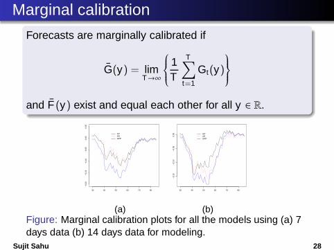
Marginal calibration

Forecasts are marginally calibrated if

G(y) = limT→∞

1T

T∑

t=1

Gt(y)

and F (y) exist and equal each other for all y ∈ R.

30 40 50 60 70 80

−0.

20−

0.15

−0.

10−

0.05

0.00

0.05

GPARGPP

(a)

30 40 50 60 70 80

−0.

15−

0.10

−0.

050.

00 GPARGPP

(b)Figure: Marginal calibration plots for all the models using (a) 7days data (b) 14 days data for modeling.

Sujit Sahu 28

Results from a large test data set

*

***

**

**** *

*

**

*

*

**

*

*

*

*

*

**

*

*

*

**

*

*

*

**

**

*

**

*

*

*

**

*

*

**

**

****

*

*

*

*

**

*

**

*

*

*

***

*

*****

*

*

*

*

***

*

**

*

**

*

*

*

*

*

*

*

*

*

*

**

*

*

*

*

****

*

*

**

***

*

***

**

*

*

**

*

*

*

*

*

*

***

*

****

*

*

*

*

*

*

*

*

*

*

*

*

*

**

**

*

*

***

*

*

*

*

*

*

**

***

**

*

**

*

*

*

*

*

****

*

*

*

**

*

*

**

**

*

*

*

*

**

**

*

*

**

*

***

*

*

*

*

**

*

*

*

**

*

**

*

*

*

*

*

*

*

*

**

*

*

*

*

*

*

*

*****

*

*

*

*

*

*

**

*

**

*

*

*

**

*

*

*

*

*

*

*

*

*

***

*

**

*

**

*

**

*

*

*

*

*

*

*

*

*

*

*

*

*

**

**

*

*

**

*

*

*

*

*

*

*

*

**

*

*

*

*

*

*

*

*

*

*

*

*

*

**

**

*

*

*

**

*

*

*

*

*

*

*

*

**

**

*

*

*

*

*

*

*

**

*

*

*

*

*

*

*

*

*

**

*

**

*

****

*

*

*

*

*

*

**

*

*

*

*

**

*

*

*

*

*

***

*

*

*

**

*

*

*

****

*

*

*

*

*

*

*

*

*

*

**

**

*

*

*

**

*

**

*

*

**

*

**

*

*

*

*

*

**

**

*

**

*

*

*

**

*

*

*

*

*

*

*

*

**

*

*

*

*

*

*

*

*

*

*

*

**

**

**

*

*

*

*

*

*

*

*

****

*

*

*

*

*

*

*

**

*

*

*

*

*

***

***

*

*

**

*

*

*

*

***

**

*

*

*

**

*

*

*

*

*

*

**

*******

**

**

*

*

***

**

****

**

** ******

+

+

+

++

+

++

+

++

+++

++

++

+

+

+

+

+

+

+

+

+

+

+

+ +

+

+

+

+

+

+

++

+

++

+

++

+

++++

+

+

++

+

+

+

+

+

++

+

*+

Fitted locationsValidation locations

Have data from639 sites in theeastern US.

We set aside 62sites for validation.

Daily data for 3weeks; June 24 toJuly 14, 2010.

We only use the GPP based approximation method.

But we will compare with the Eta-CMAQ forecasts.

Sujit Sahu 29

Validation results

Forecast 7/8 7/9 7/10 7/11 7/12 7/13 7/14 7/(8-14)Nominal coverage of the 95% forecast intervals using the linear model

7 Days 99.94 99.80 99.44 100.00 100.00 99.07 98.15 99.1114 Days 99.94 98.50 97.59 100.00 100.00 97.50 98.15 98.64

Nominal coverage of the 95% forecast intervals using the GPP model7 Days 93.55 93.75 94.96 95.16 94.96 93.75 95.56 94.5314 Days 94.62 94.30 94.84 95.05 94.62 94.84 94.84 94.74

CRPS values7 Days 10.05 7.98 6.52 6.79 7.12 7.18 7.11 7.5414 Days 9.43 7.25 5.89 6.80 6.93 6.94 6.74 7.15

Table: Nominal coverages of the 95% forecast intervals usingthe linear and GPP models and the CRPS values for the holdout data for the GPP model for the whole eastern US data set.

Sujit Sahu 30

Illustrative forecast maps

30

40

50

60

70

38.1

3836

43.8

42.7

40.7

38.5

32

38.8

54

38.5

35.9

42.8

51.5

43.7

21.6

39.3

44.6

35.6

17.9

24

25.1

41.4

2431.2

44

48

35.8

46

49.3

34

35.9

33.4

30.4

32.6

23.7

66.8

49

28.9

17.3

75.4

36.1

30.9

42

74.9

65.2

58.9

40.5

71.1

80.1

62.6

68.2

60.4

59.3

83.4

80.5

64.4

67.4

57

64.9

52.3

77.5

39.2

71.4

68.5

55.2

43.5

43.1

80.2

71.1

36.3

49.6

74.4

37.8

60.2

67.5

47.6

45.6

53.8

46.1

33.6

8 July

(a) Forecast

6.0

6.5

7.0

7.5

8.0

8.5

9.0

8 July

(b) sd

35

40

45

50

55

60

43

4446.9

49.8

45.8

45

43.3

45.5

45.5

46.1

41.5

44.5

43.8

48.2

45.3

46

44.2

41.8

55.6

49.3

41.2

23.5

50.8

20.230.9

44.2

43.1

30.6

47.5

48.4

53.1

59.2

22.4

37.6

64.7

38.5

51.9

55.4

41.5

38.7

51.3

37

44

50.1

50.4

47.8

31.4

26.2

45.5

39.6

42.8

46.5

37.7

32

51.8

46.6

41.3

44.7

44.7

44.3

41.9

49.6

12.8

46.6

46.3

53.6

44.1

35.6

44.3

62.1

33.6

38.1

58

26

52.9

48.7

41.6

41.1

58.6

52.7

52.9

10 July

6.5

7.0

7.5

8.0

8.5

10 July

Sujit Sahu 31

Benchmarking forecasts for hourly data

++ +

++

+

+

+

+

++

++ + + +

+

+

+

++ +

++ + +

++

+

+

+

++

++ +

++

+

+

+

+

+ +

++ + + + + +

++

+ +

+ + + + + + + ++

+ +

+ + + + ++

+

++

++

6 8 10 12 14 16

510

1520

25

Hour of Day (EDT)

RMSE

*

*

*

** *

* * * **

*

*

** * * * * * * **

**

* * * * * * * *

*

*

*

* * * * * ** *

*

**

** *

* * **

*

**

** *

* * ** * *

**

** *

* *

*

* *

*

aa a

a

a

a

a

a

a aa

aa a

aa

a

aa

a a a

aa a

aa

aa

aa a a

aa a

a

a

a

a

a

a aa

a

aa

a

aa

aa a

aa

aa

aa

a a aa a a

a

a a a a a a a

a

aa a

+a

*

CMAQRegressionBayes

Forecasted 11 8−h averages in 694 sites during July 8−14, 2010.

Used data from the last 7−days upto 3−hours before the forecasted hour

Root Mean Square Errors (RMSE) of real timeforecasts for 8-hr averages.

Sujit Sahu 32

Discussion

The R package spTimer implementing the methodsare now available from CRAN.

Need high resolution spatio-temporal models for awide range of data analysis problems.

Automatic non-statistical models are not likely to workunless validated by empirical data!

There is huge potential for developing methods formultivariate space-time modeling and forecasting,

These multivariate methods can be used to learnabout uncertainty of composite measures, such asany combined air quality index.

Sujit Sahu 33