Spatial Smoothing in fMRI using Prolate Spheroidal Wave Functions
Martin A. Lindquist1 and Tor D. Wager2
1 Department of Statistics, Columbia University, New York, NY, 10027
2 Department of Psychology, Columbia University, New York, NY, 10027
ADDRESS:
Martin Lindquist
1255 Amsterdam Ave, 10th Floor, MC 4409
New York, NY 10027
Phone: (212) 851-2148
Fax: (212) 851-2164
E-Mail: [email protected]
RUNNING TITLE: Spatial Smoothing using Prolate Spheroidal Wave Functions
2
ABSTRACT
The acquisition of functional magnetic resonance imaging (fMRI) data in a finite subset of k-space
produces ring-artifacts and ‘side lobes’ that distort the image. In this paper, we explore the consequences of
this problem for functional imaging studies, which can be considerable, and propose a solution. The
truncation of k-space is mathematically equivalent to convolving the underlying “true” image with a
sinc function whose width is inversely related to the amount of truncation. Spatial smoothing with a
large enough kernel can eliminate these artifacts, but at a cost in image resolution. However, too
little spatial smoothing leaves the ringing artifacts and side lobes caused by k-space truncation intact,
leading to a decrease in signal-to-noise ratio and statistical power. Thus, to make use of the high-resolution
afforded by MRI without introducing artifacts, new smoothing filters are needed that are optimized to
correct k-space truncation-related artifacts. We develop a prolate spheroidal wave function (PSWF) filter
designed to eliminate truncation artifacts and compare its performance to the standard Gaussian filter in
simulations and analysis of fMRI data on a visual-motor task. The PSWF filter effectively corrected
truncation artifacts and resulted in more sensitive detection of visual-motor activity in expected brain
regions, demonstrating its efficacy.
Key Words: fMRI, spatial smoothing, prolate spheroidal wave function, Gaussian smoothing,
preprocessing, spatial filtering
3
Introduction
In functional magnetic resonance imaging (fMRI) studies it is common practice to spatially
smooth the acquired data prior to performing statistical analysis. Spatial smoothing involves blurring the
functional MRI images by convolving the image data with a filter kernel, most frequently a Gaussian,
though other types of kernels (e.g. sinc kernel) may also be used. Gaussian smoothing is implemented in
major software packages such as SPM (Statistical Parametric Mapping, Wellcome Institute of Cognitive
Neurology, University College London), AFNI (Analysis of Functional Imaging Data), and FSL (FMRIB
software library, Oxford). It is used primarily to minimize the errors in group analysis introduced in the
spatial normalization of brains into a common space and to make data conform to the assumptions of
Gaussian Random Field Theory if it is used for correction for multiple comparisons (Worsley and Friston,
1995). In addition, if the spatial extent of a region of interest (ROI) is larger than the spatial resolution,
smoothing may reduce random noise in individual voxels and increase the signal-to-noise ratio (SNR)
within the ROI (Rosenfeld and Kak, 1982; Smith, 2003). Although it is advantageous to smooth data for
these reasons, there are also obvious costs in spatial resolution. With larger sample sizes, higher field
strengths, and other advances in imaging technology, many groups may wish to take advantage of the
high potential spatial resolution of fMRI data and minimize the amount of smoothing.
However, there is a cost to not smoothing images that is perhaps under-appreciated. The cost
comes from the fact that data are acquired in a finite portion of k-space, which is often quite limited in
functional (T2*) acquisition schemes. In order to obtain a “perfect” reconstruction of an image, an infinite
number of k-space measurements need to be made. The restriction of sampling to a finite space introduces
blurring in the image: this truncation is mathematically equivalent to convolving the image with a sinc
function whose width is inversely related to the amount of k-space that is sampled. The result is ringing
artifacts and side lobes—aliased portions of the image that extend beyond the actual location of the
imaged object—that distort the images (Fig. 1B). Such artifacts, if significantly large, may at best reduce
signal to noise ratio, and at worst result in mis-localization of functional activation.
4
Spatial smoothing of images (e.g., with a Gaussian filter) can ameliorate these problems. The
process of spatial smoothing is equivalent to applying a low-pass filter to the sampled k-space data. It has
the effect of altering the spatial resolution in the image, as it reduces the intensity of high-frequency
points in k-space, as well as changing the image’s resulting point-spread function. If the frequencies
sampled in the images are higher than the filter cutoff, the high frequency information (i.e., fine spatial
resolution) will be lost, though the side lobes will be eliminated (Fig. 1D). Alternatively, if the
frequencies sampled are lower than those in the filter, direct application of the filter will not be able to
completely eliminate the side lobes. In this case, k-space is insufficiently sampled to support the applied
filter and significant truncation artifacts will remain (Fig. 1C). The effective smoothing applied to the
images will therefore be wider than intended. Thus, when image data are rather coarsely sampled (e.g.
64×64 3.75 mm voxels in a 240 mm field of view) special care needs to be taken to minimize truncation
artifacts. In this paper we show that in certain situations a Gaussian filter will not allow for control for
these serious effects and should not be used when applying a narrow filter (e.g. with FWHM < 8 mm) to a
low resolution (e.g. 64×64) image. We show in a series of simulations that failure to take proper care of
these issues will lead to a decrease in signal-to-noise ratio and to decreased power in the resulting
statistical tests.
In principal, one can make a distinction between two separate, but related, preprocessing steps.
The first is the need to correct artifacts due to the reconstruction of finite k-space data, and the second is
smoothing as a means of increasing signal-to-noise and validating certain statistical techniques. While,
most smoothing kernels are designed primarily to deal with the latter issue, they can if properly designed
also be used to handle the former. One method that is well-suited to controlling truncation artifacts is the
0th order prolate spheroidal wave function (PSWF) (Slepian and Pollak, 1961; Landau and Pollak, 1961,
1962). The PSWF is the function, with compact support on a fixed subset of k-space, which maximizes
the signal over a certain predefined subset of image-space. Computationally, this function is the largest
eigenfunction of the finite, or truncated, Fourier transform. It should be noted that discrete prolate
5
spheroidal sequences (Slepian and Pollak, 1961) have previously appeared in the fMRI literature as
part of the multitaper technique for temporal smoothing (Mitra et. al., 1997; Mitra and Pesaran,
1999). The attractive features of the PSWF spatial smoothing filter are discussed in this paper.
Simulations show that the power to detect activation is significantly increased when using the PSWF filter
instead of a Gaussian filter if the FWHM is below 8 mm. Further data from a visual task is used to
illustrate its efficiency when applied to fMRI data.
In this work we will focus on comparing the PSWF filter with its Gaussian counterpart. However,
it is important to note that a number of other studies have been concerned with finding alternatives to
smoothing with a fixed Gaussian filter. For example, statistical analysis frameworks using Gaussians of
varying width (Poline and Mazoyer, 1994; Worsley et. al., 1996) and rotations (Shafie et. al., 2003) have
been proposed. As an alternative to using a Gaussian kernel, a number of papers have suggested the use of
wavelets (see Van De Ville et al. (2006) for an excellent overview of the literature). In addition, data-
dependent smoothing methods have also been suggested. One promising example is the use of anisotropic
diffusion (Kim et. al., 2005). It should be noted that while the approach we are suggesting is data-
independent, as are both the Gaussian and wavelet techniques, it does depend on the acquisition
parameters.
Methods
Theory
Spatial smoothing. Spatial smoothing involves blurring the functional MRI images by applying a moving
average filter to the images. When smoothing an image, each voxel is effectively transformed into the
weighted sum over a region of interest (ROI), which consists of the voxels lying under the kernel of the
filter. The size of the kernel is determined by the full width at half maximum (FWHM), which measures
the width of the kernel at 50 percent of its peak value. Hence, voxels that lie within the range defined by
the FWHM are weighted higher than voxels lying outside of this range.

6
To carry out spatial smoothing in MRI, a smoothing matrix, representing the filter, is constructed
which has the same size as the image. The image matrix is convolved with the smoothing matrix by first
Fourier transforming both the image and the smoothing matrix, and then calculating the inverse Fourier
transform of the product of these two matrices. The process of convolving the image using a smoothing
kernel can be written as
∫∫ΩΩ
=−=*
)(ˆ)(ˆ)()()(~ kkkuuxux xk deKFdKFF i , [1]
where )(xK is the smoothing matrix, )(ˆ kK its Fourier transform, )(ˆ kF is the experimental sampling
function in k-space and F(x) is its corresponding inverse Fourier transform (the image). Here )(~ xF
represents the value of the smoothed data at the coordinate point, x , of the image.
Typically when performing spatial smoothing in fMRI one uses a Gaussian kernel, though other
choices are also possible. However, due to the popularity of the Gaussian we will concentrate on studying
its properties in this particular paper. It can be expressed on the form:
⎭⎬⎫
⎩⎨⎧−∝Φ 2
2
2exp)(
σxxK . [2]
Convolving the image using the Gaussian kernel is equivalent to multiplying the k-space data by the
Fourier transform of the kernel function, which in turn can be written as:
( )⎭⎬⎫
⎩⎨⎧−∝Φ
22221exp)(ˆ kk πσK . [3]
Studying the Fourier transform of the Gaussian in Eq. [3], it is clear that it also follows a Gaussian
distribution, in this case with a standard deviation equal to 1)2( −πσ .
The width of the smoothing kernel is determined by the amount of spatial smoothing required and
is written in terms of the FWHM. It is important to note that the relationship between the FWHM and the
standard deviation of the Gaussian can be written as
)2ln(22
FWHM=σ . [4]

7
Fig. 2A (first and second row - right column) shows an example of )(xΦK and )(ˆ kΦK in one dimension.
By studying the shape of )(ˆ kΦK it is clear that application of this filter devalues points in the outer
regions of k-space and is therefore equivalent to low-pass filtering.
A well known fact about the Gaussian distribution states that 99.7% of its mass is contained in a
region lying within 3 standard deviations of its mean. Due to the symmetric nature of the Gaussian, this
region will make up a circular shape in two dimensions (spherical in three dimensions). Hence, 99.7% of
the mass of ˆ K Φ(k) will lie within a circular region with radius ( ) 123 −πσ . Using this property, we can
define an alternative measure for the extent of a filter. Let the width of the kernel in k-space be defined as
W, if 99.7% of the kernels mass lies in the range ]5.0,5.0[ WW− . Though the support of the Gaussian is
infinite, the width of ˆ K Φ(k) is related to the FWHM by Eq. [4] and can be expressed as
FWHM
W 1)2ln(26π
= . [5]
Similarly, we can define the width of the filter, )(xΦK , in image-space as T, if 99.7% of the kernels mass
in image-space lies in the range ]5.0,5.0[ TT− . Hence, the width can be expressed using Eq. [4] as
)2ln(2
3FWHMT = . [6]
Effective Smoothing. As mentioned above, there is an additional source of blurring inherent in the
reconstruction of MR images. This blurring is due to the fact that sampling is performed over a
finite subset of k-space. In order to obtain a “perfect” reconstruction of the underlying image one
would need to sample an infinitely large region of k-space. Unfortunately, this is not possible and
k-space is by necessity truncated. This truncation results in a ringing artifact in the image which is
due to the under-sampling of high spatial frequency components of k-space (Fig. 1B). By
truncating k-space we are performing an operation that is mathematically equivalent to convolving
the underlying “true” image with a sinc function, whose width is inversely related to the amount of
truncation. It should be noted that throughout this paper we are assuming that we are dealing with images
8
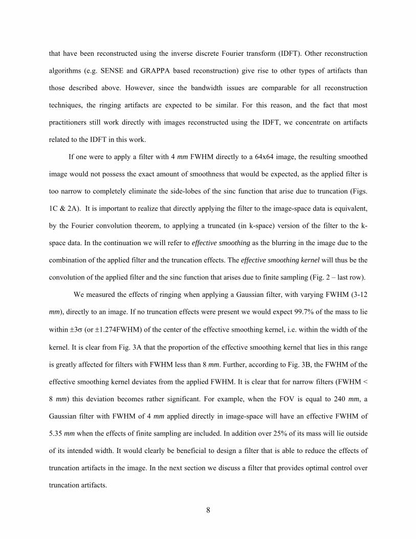
that have been reconstructed using the inverse discrete Fourier transform (IDFT). Other reconstruction
algorithms (e.g. SENSE and GRAPPA based reconstruction) give rise to other types of artifacts than
those described above. However, since the bandwidth issues are comparable for all reconstruction
techniques, the ringing artifacts are expected to be similar. For this reason, and the fact that most
practitioners still work directly with images reconstructed using the IDFT, we concentrate on artifacts
related to the IDFT in this work.
If one were to apply a filter with 4 mm FWHM directly to a 64x64 image, the resulting smoothed
image would not possess the exact amount of smoothness that would be expected, as the applied filter is
too narrow to completely eliminate the side-lobes of the sinc function that arise due to truncation (Figs.
1C & 2A). It is important to realize that directly applying the filter to the image-space data is equivalent,
by the Fourier convolution theorem, to applying a truncated (in k-space) version of the filter to the k-
space data. In the continuation we will refer to effective smoothing as the blurring in the image due to the
combination of the applied filter and the truncation effects. The effective smoothing kernel will thus be the
convolution of the applied filter and the sinc function that arises due to finite sampling (Fig. 2 – last row).
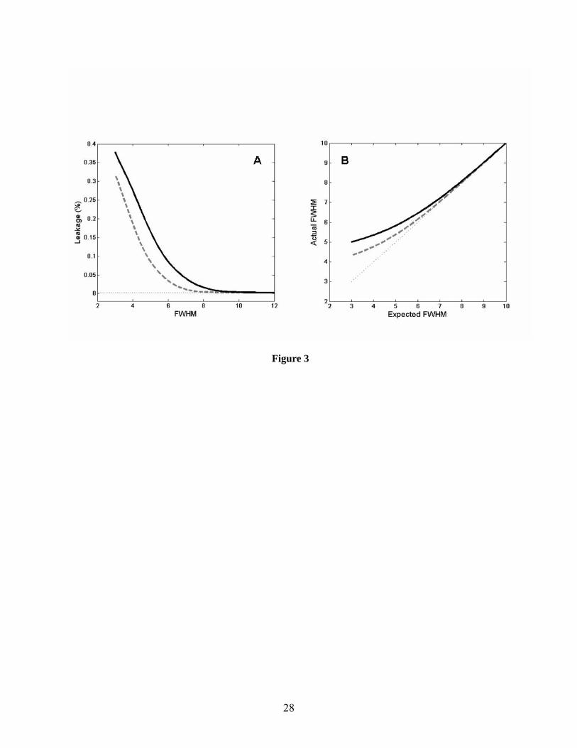
We measured the effects of ringing when applying a Gaussian filter, with varying FWHM (3-12
mm), directly to an image. If no truncation effects were present we would expect 99.7% of the mass to lie
within ±3σ (or ±1.274FWHM) of the center of the effective smoothing kernel, i.e. within the width of the
kernel. It is clear from Fig. 3A that the proportion of the effective smoothing kernel that lies in this range
is greatly affected for filters with FWHM less than 8 mm. Further, according to Fig. 3B, the FWHM of the
effective smoothing kernel deviates from the applied FWHM. It is clear that for narrow filters (FWHM <
8 mm) this deviation becomes rather significant. For example, when the FOV is equal to 240 mm, a
Gaussian filter with FWHM of 4 mm applied directly in image-space will have an effective FWHM of
5.35 mm when the effects of finite sampling are included. In addition over 25% of its mass will lie outside
of its intended width. It would clearly be beneficial to design a filter that is able to reduce the effects of
truncation artifacts in the image. In the next section we discuss a filter that provides optimal control over
truncation artifacts.

9
The Prolate Spheroidal Wave Function Filter. The prolate spheroidal wave function (PSWF) filter is
the function, with compact support on a fixed set of k-space, which maximizes the signal over a certain
predefined subset of image-space. To find this function, we begin by setting up the problem formulation.
As k-space consists of a sequence of discrete measurements during MRI data acquisition, it should
therefore be chosen to be a discrete space. On the other hand, image-space, denoted by Ω in this paper,
can be chosen to be either a discrete space consisting of a collection of the image voxels (e.g.
the NN × voxels in an image) or as a continuous space. We discuss the latter below. Next, consider a
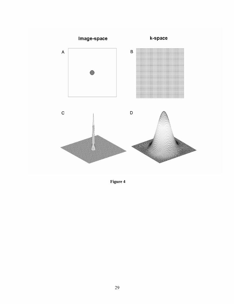
convex region of interest (ROI), denoted B, in image-space and the k-space sampling region, A (e.g. the
collection of measured points on a 64×64 grid –see Fig. 4A-B). The objective is to find the filter function
g(k), that satisfies the following two criteria:
1. It takes the value 0 for points outside of A.
2. Its inverse Fourier transform, G(x), has maximal signal concentration in B, i.e. the ratio
(7)
is maximized over all possible functions for which the first criterion holds.
These conditions ensure that g(k) is the function with compact support on A, whose inverse Fourier
transform has the least amount of signal leakage outside of the region B. Thus, it is the function with
optimal control over ringing artifacts outside of B. Note that λ takes values between 0 and 1 and can be
interpreted as the amount of signal leakage that the filter gives rise to outside of the predetermined ROI B.
As an additional constraint, the denominator of the ratio in Eq. 7 is set equal to one. This simplifies
the problem to finding the function, g(k), with norm equal to one, whose inverse Fourier transform
maximizes,
∫
∫
Ω
=xx
xx
dG
dGB
2
2
|)(|
|)(|λ
10
∫=B
dG xx 2)(λ . (8)
Using Parseval’s identity, the problem can be written in matrix form as,
gKg Bˆmax +=λ (9)
under the constraint,
1)()(j
jj == ∑∈
+
A
ggk
kkgg . (10)
Let us define BK to be the Fourier transform of the indicator function of the region B, which can be
written:
∫ −=B
B diK xkxk ),(2exp)(ˆ π (11)
Then it can be shown (Yang et al, 2002; Lindquist, 2003; Lindquist et al, 2006) that the kernel, BK , is
given by,
)'(ˆ)',(ˆ kkkkK −= BB K (12)
for k, k ' ∈ A. A more detailed derivation of these results can be found in the Appendix. For simple
regions B (e.g. circles, squares, ellipses) there exist analytical expressions for BK , which allow for easy
computation of the kernel defined in Eq. 12.
The kernel BK is positive definite which implies that all of its eigenvalues kλ , 1,0 −= ak K , are
non-negative, where a denotes the number of points sampled in k-space (e.g. 2Na = ). In fact,
01 110 ≥≥≥≥≥ −aλλλ K . (13)
The eigenfunction, g0, associated with the largest eigenvalue, 0λ , is termed the 0-order solution, and
provides the solution to the problem stated in Eq. 7. In addition, 0λ is equal to the fraction of the total
signal intensity in B calculated according to Eq. 7 and provides a quantitative measure of the signal

11
leakage that the eigenvector gives rise to. A value of 0λ close to 1 indicates little signal leakage, while
the leakage increases as 0λ decreases. The set of eigenfunctions 110 ,, −aggg K have some interesting
properties. As we will always choose A to be symmetrical about the center of k-space (k=0), the set of
eigenvectors can always be taken to be real and orthogonal on B. In addition, the index i not only ranks
the eigenvalues, but also specifies the number of zeros the function ig has within the region B (Percival
and Walden, 1993). The function g0 will therefore be positive over the whole region B, a property it
shares with the Gaussian kernel.
By applying the filter g(k) directly to the k-space data and thereafter taking the inverse Fourier
transform of the filtered k-space data, the resulting image will represent the true image convolved with
the function G(x). Therefore the PSWF can be used as a filter to spatially smooth fMRI data. The amount
of smoothing applied will depend upon the size of the region B. In our discussion of the PSWF filter it
will often make more sense to talk about the filters width instead of the traditional FWHM used for the
Gaussian. As long as 997.0≥λ , the width of the PSWF is bounded by the diameter of the region B, as
this condition ensures that less than 0.3% of the signal lies outside of B. The PSWF filter has the
important property that any other choice of filter will give rise to a greater amount of signal leakage
outside of the spatial coverage region. Hence, the PSWF filter is chosen to minimize the amount of signal
leakage, and thereby ringing, outside of the region B. This property leads us to believe that it has excellent
potential as a spatial smoothing filter in fMRI.
In practice, one can construct a smoothing kernel by taking the IDFT of g(k) and reconstructing it
onto a matrix with the same dimensions as the image. Smoothing can thereafter be performed in an
analogous manner as for Gaussian, which is described algebraically in Eq. 1. In our implementation, A is
chosen to correspond to the sampled region of k-space (Fig. 4B) and B is chosen to be a circular region
with diameter 1.274FWHM (equal to 6σ) to ensure a kernel with similar width as a Gaussian filter of a
given FWHM. Figs. 4C-D show examples of G(x) and g(k) corresponding to the regions A and B. The
PSWF filter shares many of the same qualities as the Gaussian filter. However, it is completely
12
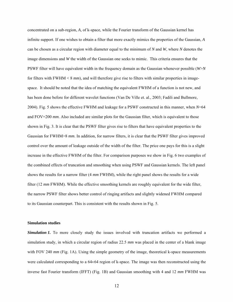
concentrated on a sub-region, A, of k-space, while the Fourier transform of the Gaussian kernel has
infinite support. If one wishes to obtain a filter that more exactly mimics the properties of the Gaussian, A
can be chosen as a circular region with diameter equal to the minimum of N and W, where N denotes the
image dimensions and W the width of the Gaussian one seeks to mimic. This criteria ensures that the
PSWF filter will have equivalent width in the frequency domain as the Gaussian whenever possible (W>N
for filters with FWHM < 8 mm), and will therefore give rise to filters with similar properties in image-
space. It should be noted that the idea of matching the equivalent FWHM of a function is not new, and
has been done before for different wavelet functions (Van De Ville et. al., 2003; Fadili and Bullmore,
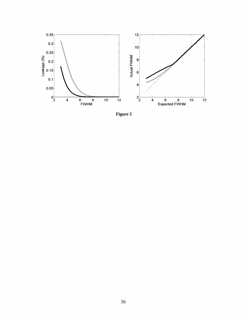
2004). Fig. 5 shows the effective FWHM and leakage for a PSWF constructed in this manner, when N=64
and FOV=200 mm. Also included are similar plots for the Gaussian filter, which is equivalent to those
shown in Fig. 3. It is clear that the PSWF filter gives rise to filters that have equivalent properties to the
Gaussian for FWHM>8 mm. In addition, for narrow filters, it is clear that the PSWF filter gives improved
control over the amount of leakage outside of the width of the filter. The price one pays for this is a slight
increase in the effective FWHM of the filter. For comparison purposes we show in Fig. 6 two examples of
the combined effects of truncation and smoothing when using PSWF and Gaussian kernels. The left panel
shows the results for a narrow filter (4 mm FWHM), while the right panel shows the results for a wide
filter (12 mm FWHM). While the effective smoothing kernels are roughly equivalent for the wide filter,
the narrow PSWF filter shows better control of ringing artifacts and slightly widened FWHM compared
to its Gaussian counterpart. This is consistent with the results shown in Fig. 5.
Simulation studies
Simulation 1. To more closely study the issues involved with truncation artifacts we performed a
simulation study, in which a circular region of radius 22.5 mm was placed in the center of a blank image
with FOV 240 mm (Fig. 1A). Using the simple geometry of the image, theoretical k-space measurements
were calculated corresponding to a 64×64 region of k-space. The image was then reconstructed using the
inverse fast Fourier transform (IFFT) (Fig. 1B) and Gaussian smoothing with 4 and 12 mm FWHM was

13
applied to the resulting images. In addition, a PSWF filter with the same width as the Gaussian with 4 mm
FWHM was applied to the data.
Simulation 2. (Part A) The image described in the previous simulation (Fig. 1A) was recreated 160
times. In 80 of the images the intensity for voxels within the circle was set to 1.0. These images were
denoted as OFF images. In the remaining 80 images the intensity was set to 1.05. These are denoted as
ON images. The images were thereafter ordered according to the paradigm of 4 repetitions of 20 OFF/ 20
ON images and Gaussian noise was added to the data with a standard deviation corresponding to a
Cohen’s d of 0.25 (Cohen, 1988). Theoretical k-space measurements were calculated corresponding to a
64×64 region of k-space and the images were reconstructed at this resolution using the IFFT. The
resulting data was smoothed using both PSWF and Gaussian filters with FWHM equal to 4, 8 and 12 mm.
The resulting data was analyzed using the standard GLM approach. This procedure was repeated 1000
times and the statistical power to detect activation was calculated for each filter type and width. (Part B)
The procedure outlined in part A was repeated using a more realistic activation pattern (Fig. 8B). Using a
grey matter mask a region of activity was created. The resulting data was interpolated to 10 times its size
(640×640) and the fast Fourier transform was used to calculate k-space data. The central 64×64 region
was used in order to mimic the effects of finite k-space sampling. Using this data set the same
experimental paradigm as described in (A), with 4 repetitions of 20 OFF/ 20 ON images, was created. The
data was analyzed in an analogous manner as described in part A.
Experiment
Nine students at the University of Michigan were recruited and paid $50 for participation in the
study. All human participant procedures were conducted in accordance with Institutional Review Board
guidelines. The experimental data consisted of a visual paradigm conducted on the 9 subjects. It
consisted of a blocked alternation of 11 s of full-field contrast-reversing checkerboards (16 Hz) with 30 s
of open-eye fixation baseline. Blocks of unilateral contrast-reversing checkerboards were presented on an
14
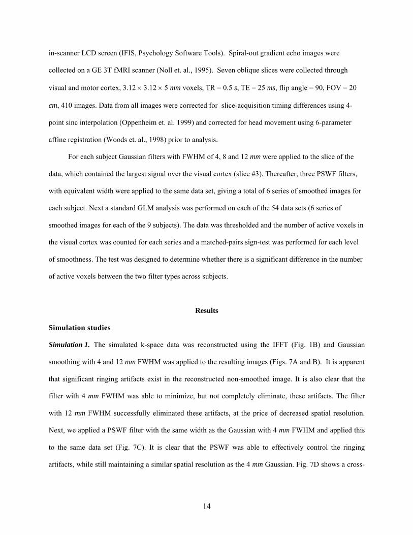
in-scanner LCD screen (IFIS, Psychology Software Tools). Spiral-out gradient echo images were
collected on a GE 3T fMRI scanner (Noll et. al., 1995). Seven oblique slices were collected through
visual and motor cortex, 3.12 × 3.12 × 5 mm voxels, TR = 0.5 s, TE = 25 ms, flip angle = 90, FOV = 20
cm, 410 images. Data from all images were corrected for slice-acquisition timing differences using 4-
point sinc interpolation (Oppenheim et. al. 1999) and corrected for head movement using 6-parameter
affine registration (Woods et. al., 1998) prior to analysis.
For each subject Gaussian filters with FWHM of 4, 8 and 12 mm were applied to the slice of the
data, which contained the largest signal over the visual cortex (slice #3). Thereafter, three PSWF filters,
with equivalent width were applied to the same data set, giving a total of 6 series of smoothed images for
each subject. Next a standard GLM analysis was performed on each of the 54 data sets (6 series of
smoothed images for each of the 9 subjects). The data was thresholded and the number of active voxels in
the visual cortex was counted for each series and a matched-pairs sign-test was performed for each level
of smoothness. The test was designed to determine whether there is a significant difference in the number
of active voxels between the two filter types across subjects.
Results
Simulation studies
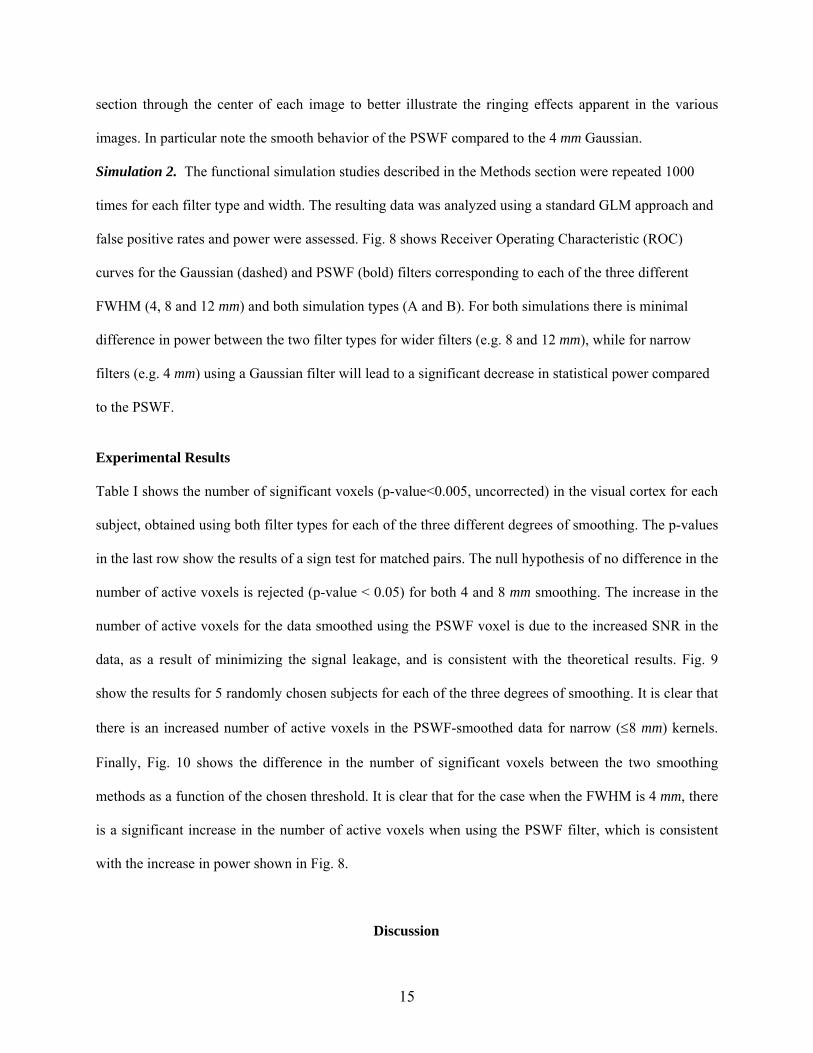
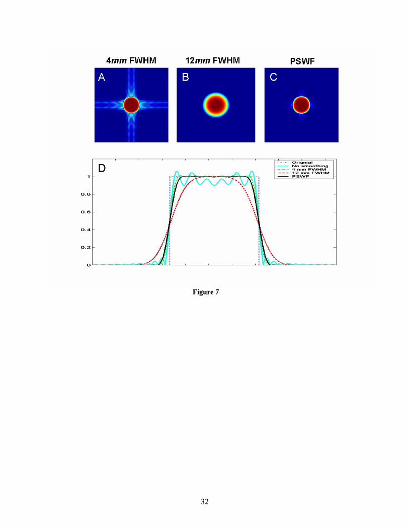
Simulation 1. The simulated k-space data was reconstructed using the IFFT (Fig. 1B) and Gaussian
smoothing with 4 and 12 mm FWHM was applied to the resulting images (Figs. 7A and B). It is apparent
that significant ringing artifacts exist in the reconstructed non-smoothed image. It is also clear that the
filter with 4 mm FWHM was able to minimize, but not completely eliminate, these artifacts. The filter
with 12 mm FWHM successfully eliminated these artifacts, at the price of decreased spatial resolution.
Next, we applied a PSWF filter with the same width as the Gaussian with 4 mm FWHM and applied this
to the same data set (Fig. 7C). It is clear that the PSWF was able to effectively control the ringing
artifacts, while still maintaining a similar spatial resolution as the 4 mm Gaussian. Fig. 7D shows a cross-
15
section through the center of each image to better illustrate the ringing effects apparent in the various
images. In particular note the smooth behavior of the PSWF compared to the 4 mm Gaussian.
Simulation 2. The functional simulation studies described in the Methods section were repeated 1000
times for each filter type and width. The resulting data was analyzed using a standard GLM approach and
false positive rates and power were assessed. Fig. 8 shows Receiver Operating Characteristic (ROC)
curves for the Gaussian (dashed) and PSWF (bold) filters corresponding to each of the three different
FWHM (4, 8 and 12 mm) and both simulation types (A and B). For both simulations there is minimal
difference in power between the two filter types for wider filters (e.g. 8 and 12 mm), while for narrow
filters (e.g. 4 mm) using a Gaussian filter will lead to a significant decrease in statistical power compared
to the PSWF.
Experimental Results
Table I shows the number of significant voxels (p-value<0.005, uncorrected) in the visual cortex for each
subject, obtained using both filter types for each of the three different degrees of smoothing. The p-values
in the last row show the results of a sign test for matched pairs. The null hypothesis of no difference in the
number of active voxels is rejected (p-value < 0.05) for both 4 and 8 mm smoothing. The increase in the
number of active voxels for the data smoothed using the PSWF voxel is due to the increased SNR in the
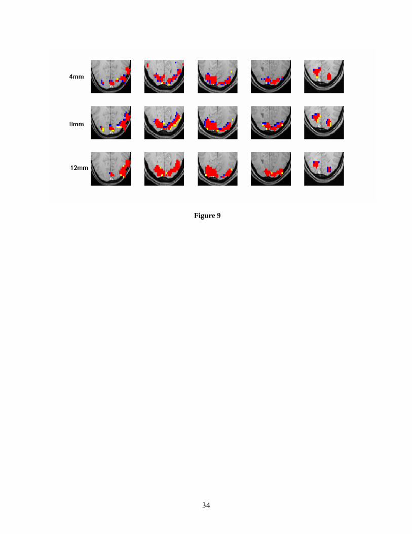
data, as a result of minimizing the signal leakage, and is consistent with the theoretical results. Fig. 9
show the results for 5 randomly chosen subjects for each of the three degrees of smoothing. It is clear that
there is an increased number of active voxels in the PSWF-smoothed data for narrow (≤8 mm) kernels.
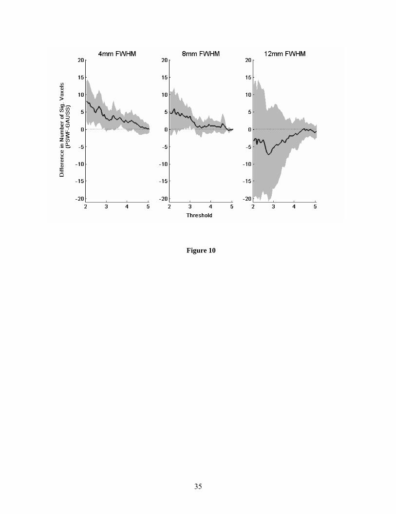
Finally, Fig. 10 shows the difference in the number of significant voxels between the two smoothing
methods as a function of the chosen threshold. It is clear that for the case when the FWHM is 4 mm, there
is a significant increase in the number of active voxels when using the PSWF filter, which is consistent
with the increase in power shown in Fig. 8.
Discussion
16
In this paper we have discussed two potential sources of blurring in fMRI data. The first is due to
the algorithm used to reconstruct the image from finite k-space data and is generally considered an
unwanted artifact of image reconstruction. The second is due to the voluntary application of a smoothing
kernel - typically used to increase SNR. The sinc function shown in Fig. 2 is the smoothing (spatial
response function) that arises when reconstruction is performed using the inverse discrete Fourier
transform (DFT). It is important to note that other reconstruction algorithms will ultimately give rise to
other spatial response functions and may therefore be more or less effective in dealing with issues such as
Gibbs ringing. For example, data obtained using parallel imaging techniques, do not reconstruct the image
using the inverse DFT. In these situations the spatial response function is much more complicated than
the sinc assumed in this paper. While the results of this paper can not be readily generalized to all
reconstruction techniques, we have ultimately decided to focus on the artifacts that arise from using the
DFT to reconstruct the images, as this is the type of data most practitioners will likely have to work with.
In addition, as each reconstruction technique is faced with the same bandwidth problems the ringing
artifacts should ultimately take a similar form. However, it should be noted that the PSWF methodology
outlined in this paper have been generalized to k-space data that is sampled on non-cartesian k-space
(Lindquist et. al., 2006). Hence, this would in principal allow for reconstruction and smoothing of data
obtained in any manner using the PSWF methodology.
In this work we have illustrated that when applying a narrow Gaussian filter (e.g. 4 mm FWHM)
to low-resolution data (e.g. 64×64), an insufficient number of measurements are made in k-space to
support the applied filter. Hence the smoothed images will contain more blurring than originally
intended and the effective smoothing will be greater than the nominally applied smoothing. The
truncation artifacts can be effectively controlled by applying a tapered filter function directly to the k-
space data. There are a number of ways of tapering the filter function. For example one can apply a
Hamming filter to the truncated Gaussian, thereby eliminating its steep edges. However, in this work we
introduce another tapered filter function, based on the theory of the prolate spheroidal wave function,
which can be used to control the amount of ringing in the resulting smoothed images. The PSWF has
17
similar properties to the Gaussian, with the added benefit that it provides optimal control over truncation
artifacts. The PSWF filter has an additional benefit that has not previously been discussed.
Throughout this paper we have defined the spatial coverage region of our filter, given by B, to be a
circular region in order to obtain an isotropic filter comparable to a Gaussian. However, it is important to
note that there is nothing in the theory of the PSWF that limits us to constructing isotropic filters, as B can
be chosen to take other shapes as well. For example, we may want to choose B to be an oval or some
other “blob-like” shape and a filter with spatial coverage corresponding to this region can be constructed
using the PSWF methodology (Yang et. al., 2002, Lindquist et. al., 2006).
In principal, the amount of smoothing applied is determined by the expected extent of activation.
By the matched filter theorem, optimal filtering is provided by using a filter with the same spatial extent
as the activation. Of course this region is never known exactly, making it difficult to determine the
optimal amount of smoothing in practice. However, it is reasonable to assume that the activation pattern
takes place in a coherent “blob” in the brain and it would be difficult to argue that the pattern would be
rippled in the manner that would be present after the application of a narrow Gaussian filter. We therefore
feel that the PSWF is more in the spirit of the matched filter theorem than the Gaussian. However, with
the introduction of high-field scanners and state-of-the-art MR imaging techniques, the “problematic”
spatial resolutions under discussion in this work (e.g. 64×64 matrix 3.75 mm resolution) may eventually
become obsolete. In these situations the advantages of the PSWF filter over the Gaussian are less clear.
On the other hand, in these situations the rational for smoothing at all is questionable.
It should be noted that the Convolution theorem (illustrated in Fig.2) only holds when the filter is
applied directly to the complex image-space data and most researchers instead work with magnitude
images. However, since the PSWF filter is positive and real-valued in our implementation (like the
Gaussian), it does not matter whether we apply the filter to the complex image-space data or to the
positive magnitude images. The results will be equivalent regardless and the Convolution theorem is still
valid. The implementation of the filter is straightforward and Matlab code is available from the authors
(www.stat.columbia.edu/~martin/Software.html). There is a one-time cost in calculating the filter

18
corresponding to a specific width, FOV and matrix size. This calculation involves calculating the largest
eigenfunction of an aa× matrix. However, if we want an n-dimensional smoothing kernel we can
approximate them as the separable product of n 1-dimensional 0-order prolate spheroidal wave functions.
This significantly simplifies calculation with minimal loss of efficiency.
Simulation studies showed an increase in power compared to Gaussian smoothing with a small
FWHM (< 8 mm). In addition, the experimental data presented in this paper clearly showed the benefits of
using a PSWF filter. In general, we feel that the increase in power shown in both simulations, in
conjunction with the increased number of activated voxels in the experimental data, together make a
strong case for the PSWF methods superiority when narrow kernels (< 8 mm) are required for smoothing
fMRI data. These results are consistent with the theory, which states that for narrow filters the PSWF has
superior concentration properties compared to the Gaussian. By applying the PSWF filter we are able to
increase the signal-to-noise by maintaining control over truncation effects.
While SNR is one important issue relating to spatial smoothing, also important are the statistical
issues of inter-subject variability and statistical validity. When using a tapered filter such as the PSWF
these issues can only be positively impacted, as a reduction of the ringing effects can only be good for the
subsequent statistical analysis, as it allows for construction of a kernel that better matches the extent of
activation. Finally, we feel that it is reasonable to assume that the PSWF filter is interchangeable to the
Gaussian in the sense that both can be used to provide the appropriate amount of smoothness needed to
make the assumptions of the random field theory valid. In determining the appropriate filter width
required for valid inference, we suggest using the same rule-of-thumb typically used for a Gaussian kernel
(e.g. 2-3 voxels).
Conclusion
In this work a new spatial smoothing filter for fMRI is introduced. The filter is based on the use
of prolate spheroidal wave functions and provides optimal control of truncation artifacts present in MR
images. The PSWF filter has the important property that any other choice of filter will give rise to a

19
greater amount of signal leakage outside of the width of the filter. This property leads us to believe that it
has excellent potential as a spatial smoothing filter in fMRI. Simulation studies showed a significant
increase in power compared to the traditionally used Gaussian filter when smoothing with narrow filters
(e.g. FWHM < 8 mm). Experimental data from a visual paradigm showed when smoothing with narrow
filters the PSWF filter gave rise to a significant rise in the number of active voxels in the visual cortex
compared to data smoothed with a comparable Gaussian filter. This rise is attributable to an increase in
signal-to-noise ratio.

20
REFERENCES
1. Cohen J 1988. Statistical power analysis for the behavioral sciences (2nd Edition), Erlbaum,
Hillsdale, NJ.
2. Fadili MJ, Bullmore ET (2004): A comparative evaluation of wavelet-based methods for hypothesis
testing of brain activation maps. NeuroImage, 23(3):1112-1128.
3. Kim HY, Giacomantone J, Cho ZH (2005): Robust anisotropic diffusion to produce enhanced
statistical parametric map from noisy fMRI. Comput. Vis. Image Underst. 99(3):435-452
4. Landau HJ, Pollak HO (1961): Prolate Spheroidal Wave Functions, Fourier Analysis and
Uncertainty, II. Bell System Tech. J., 40:65-84.
5. Landau HJ, Pollak HO (1962): Prolate Spheroidal Wave Functions, Fourier Analysis and
Uncertainty, III. Bell System Tech. J., 41:1295-1336.
6. Lindquist MA (2003): Optimal Data Acquisition in fMRI Using Prolate Spheroidal Wave Functions.
International Journal of Imaging Systems and Technology, 13:126-132.
7. Lindquist MA, Zhang C-H, Glover G, Shepp L, Yang QA (2006): Generalization of the Two
Dimensional Prolate Spheroidal Wave Function Method for Non-Rectilinear MRI Data Acquisition
Methods. IEEE Transactions in Image Processing 15(9):2792-2804.
8. Mitra PP, and Pesaran B (1999): Analysis of dynamic brain imaging data. Biophys. J., 76(2):691-708.
9. Mitra PP, Ogawa S, Hu X, and Ugurbil K (1997): The nature of spatiotemporal changes in cerebral
hemodynamics as manifested in functional magnetic resonance imaging. Magn. Reson. Med.,
37(4):511-518.
10. Noll DC, Cohen JD, Meyer CH, Schneider W (1995): Spiral K-space MR imaging of cortical
activation. J Magn Reson Imaging, 5(1):49-56.
11. Oppenheim AV, Schafer RW, Buck JR. 1999. Discrete-Time Signal Processing (2nd Edition),
Prentice Hall, Upper Saddle River, NJ.
21
12. Percival DB, Walden A. 1993. Spectral Analysis for Physical Applications, Cambridge
University Press, Cambridge, UK.
13. Poline JB, Mazoyer B (1994): Analysis of individual brain activation maps using
hierarchical description and multiscale detection. IEEE Trans. Med. Imag. 4:702– 710.
14. Rosenfeld A, Kak AC. 1982. Digital Picture Processing. Vol. 2, Academic Press, Orlando, Florida.
15. Shafie K, Sigal B, Siegmund D, Worsley K (2003): Rotation space random fields with an application
to fMRI data. Ann. Stat. 31:1732 – 1771.
16. Shepp L, Zhang CH (2000): Fast Functional Magnetic Resonance Imaging via Prolate Wavelets.
Applied and Computational Harmonic Analysis 9:99-119.
17. Slepian D, Pollak HO (1961): Prolate Spheroidal Wave Functions, Fourier Analysis and
Uncertainty, I. Bell System Tech. J. 40:43-64.
18. Smith SM (2003): Preparing fMRI data for statistical analysis. In: Jezzard P, Matthews PM, Smith
SM (Eds.), Functional MRI: an introduction to methods, Oxford University Press, Oxford, UK.
19. Van De Ville D, Blu T, Unser M (2003): Wavelets Versus Resels in the Context of fMRI:
Establishing the Link with SPM. Proceedings of the SPIE Conference on Mathematical Imaging:
Wavelet Applications in Signal and Image Processing X, San Diego (CA), 5207(I):417-425.
20. Van De Ville D, Blu T, Unser M (2006): Surfing the Brain—An Overview of Wavelet-Based
Techniques for fMRI Data Analysis. IEEE Engineering in Medicine and Biology Magazine, 25(2):65-
78.
21. Wager TD, Vazquez A, Hernandez L, Noll DC (2005): Accounting for nonlinear BOLD effects in
fMRI: parameter estimates and a model for prediction in rapid event-related studies. Neuroimage,
25(1):206-218.
22. Woods RP, Grafton ST, Holmes CJ, Cherry SR, Mazziotta, JC (1998): Automated image registration:
I. General methods and intrasubject, intramodality validation. J Comput Assist Tomogr, 22(1):139-
152.

22
23. Worsley K, Marrett S, Neelin P, Evans A (1996): Searching scale space for activation in PET images.
Hum. Brain Mapp. 4 (1):74–90.
24. Worsley KJ, Friston KJ (1995): Analysis of fMRI Time-Series revisited – Again. Neuroimage 2:173-
197.
25. Yang QX, Lindquist MA, Shepp L, Zhang CH, Wang J, Smith MB (2002): Two Dimensional Prolate
Spheroidal Wave Functions for MRI. Journal of Magnetic Resonance 158:43-51.
23
Figure Captions
FIGURE 1. (A) A circular region of radius 22.5 mm is placed in an image with FOV 240 mm and
theoretical k-space measurements are calculated corresponding to a 64x64 region of k-space. (B) Image
reconstruction with no smoothing. The ringing is due to the fact that k-space is truncated. (C) The image
in (B) is smoothed using a Gaussian filter with 4 mm FWHM. The ringing artifacts are reduced but not
completely eliminated. (D) The image in (B) is smoothed using a Gaussian filter with 12 mm FWHM.
The ringing artifacts are eliminated, at the cost of reduced image resolution. The images are plotted on the
log-scale to better illuminate the ringing artifacts.
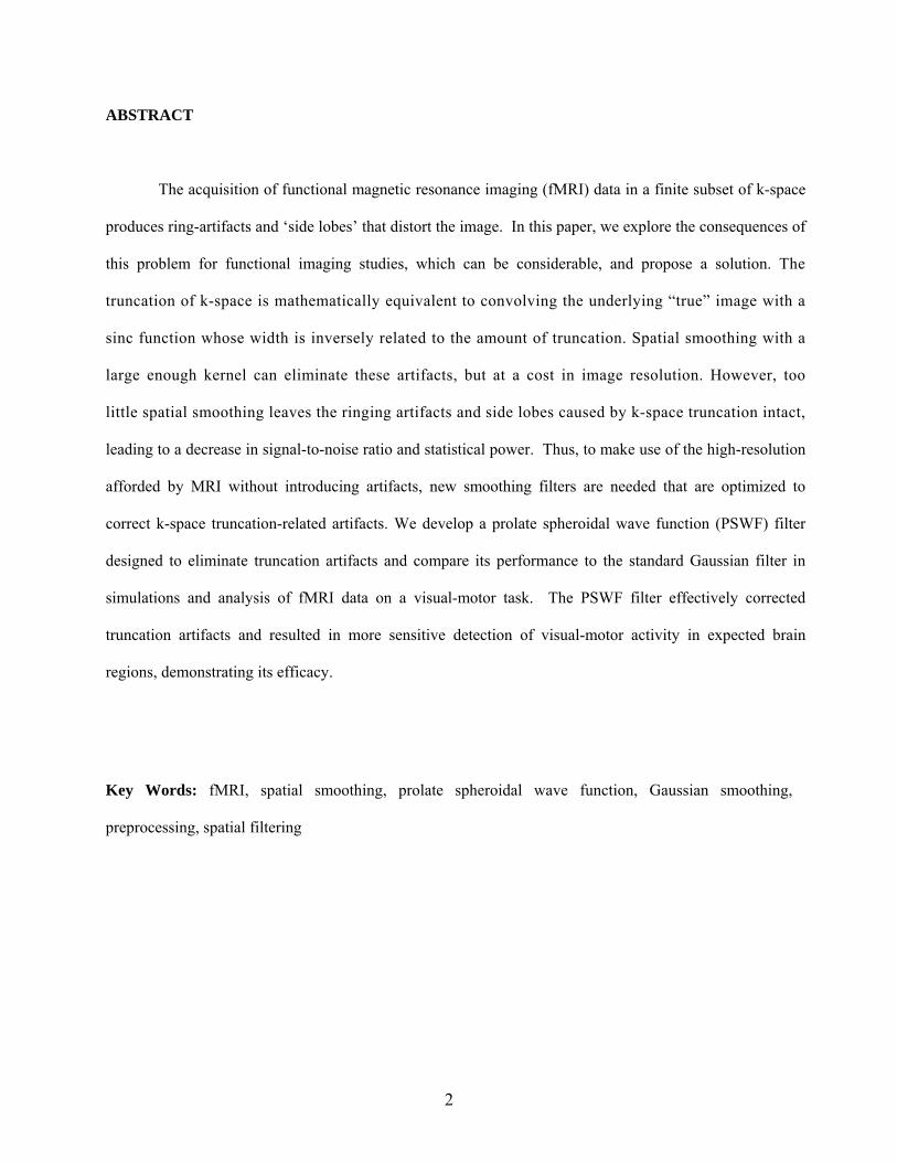
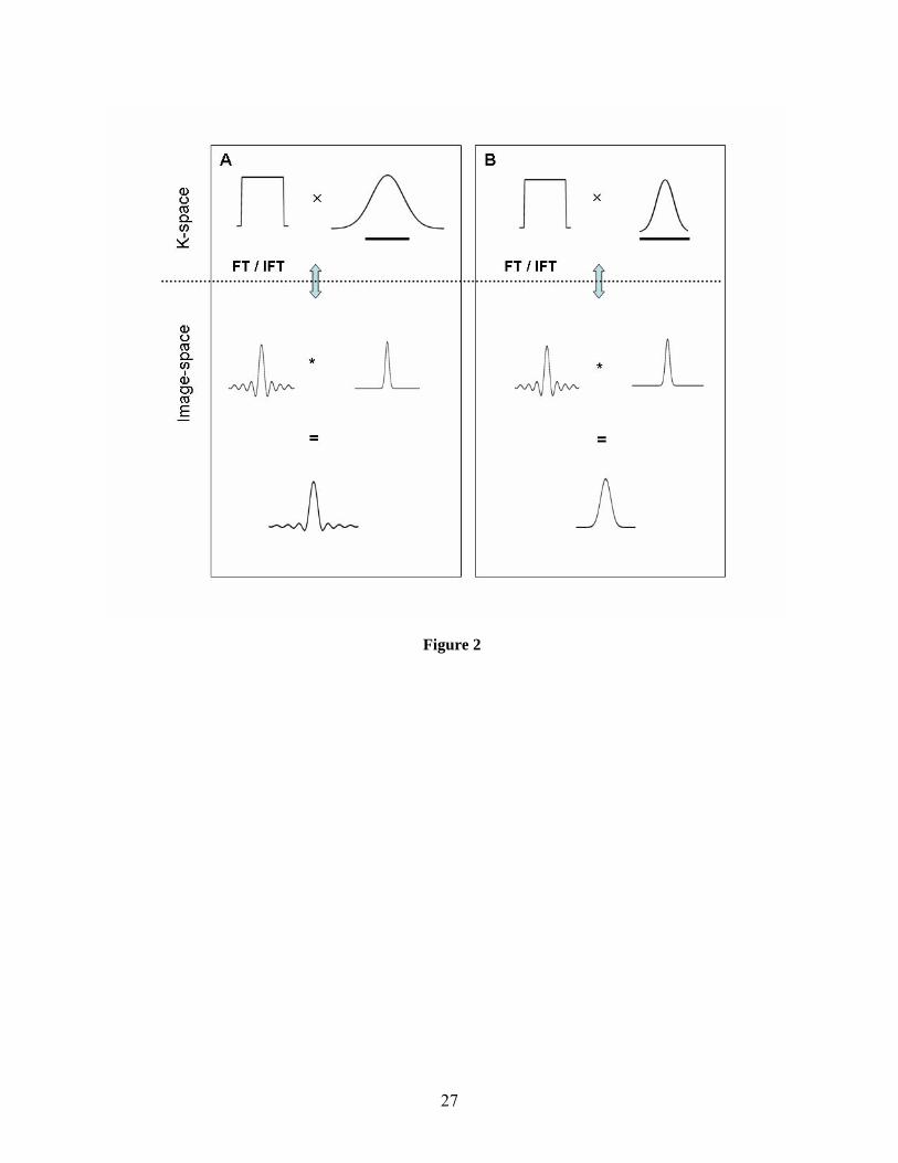
FIGURE 2. (A) A boxcar function (top left) is multiplied with a Gaussian kernel (top right). The line
under the Gaussian shows the frequency extent of the boxcar compared to the Gaussian. After performing
the inverse Fourier transform on the product, the result is equivalent by the Fourier Convolution Theorem,
to convolving the point spread function (center left) with a Gaussian kernel (center right). The results of
this convolution are shown in the bottom row. (B) A boxcar function (top left) is multiplied with a kernel
(top right) designed to have the same frequency extent as the boxcar. After performing the inverse Fourier
transform on the product, the result is equivalent to convolving the point spread function (center left) with
the inverse Fourier transform of the kernel (center right). The results of this convolution are shown in the
bottom row. The filter effectively controls for the ringing artifacts.
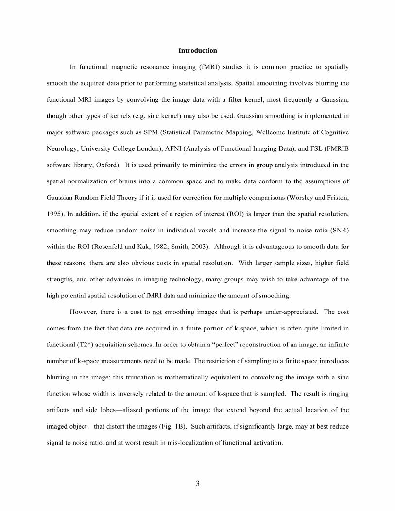
FIGURE 3. (A) The proportion of the effective Gaussian smoothing kernel that lies within ±3σ (or ±
1.274FWHM) of the center of the filter when N=64 and the FOV is equal to 200 and 240 mm (dashed and
bold line respectively). (B) The actual and expected FWHM plotted for a Gaussian filter for the case
when N=64 and the FOV is equal to 200 and 240 mm (dashed and bold line respectively). For comparison
purposes the dotted line shows where the actual and expected FWHM coincide.
24
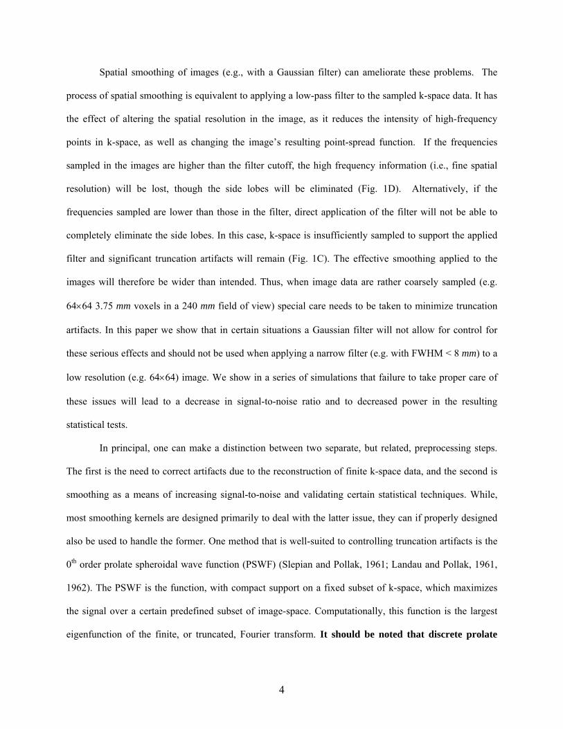
FIGURE 4. A circular region B in image-space (top left) and a k-space subset A (top right). The PSWF
filter g(k) (bottom right) and its inverse Fourier transform G(x) (bottom left) corresponding to the choice
of A and B. Note the minimal ringing present in the image-space filter.
FIGURE 5. (A) The proportion of the PSWF kernel (bold) and the Gaussian kernel (dashed) that lies
within ±3σ (or ± 1.274FWHM) of the center of the filter when N=64 and the FOV is equal to 200 mm.
(B) The actual and expected FWHM plotted for the PSWF and Gaussian filter for the case when N=64
and the FOV is equal to 200 mm (bold and dashed line respectively). For comparison purposes the dotted
line shows where the actual and expected FWHM coincide.
FIGURE 6. The effective smoothing kernel obtained using the PSWF (bold) and the Gaussian (dashed)
with 4 mm (left) and 12 mm (right) FWHM (N=64, FOV=200 mm). While the filters are roughly
equivalent for the wider FWHM, the narrow PSWF filter shows better control of ringing artifacts and
slightly widened FWHM compared to its Gaussian counterpart.
FIGURE 7. The image in Fig. 1B is smoothed using a Gaussian filter with FWHM equal to (A) 4 mm
and (B) 12 mm, as well as with a PSWF with width equivalent to a 4 mm Gaussian (C). The images (A-C)
are plotted on the log-scale to better illuminate the ringing artifacts. (D) A cross-section through the
center of each image (A-C, along with Figs. 1A-B) illustrates the ringing effects apparent in each case.
FIGURE 8. (A) The simulated activation pattern and Receiver Operating Characteristic (ROC) curves
from Simulation 2A obtained using Gaussian (dashed) and PSWF (bold) filters corresponding to 3
different FWHM (4, 8 and 12 mm). For narrow filters (e.g. 4 mm) using a Gaussian filter will lead to a
significant decrease in statistical power compared to the PSWF. (B) The same results for Simulation 2B.
Analogous results hold in this situation.

25
FIGURE 9. Statistical parametric maps, obtained from 5 randomly chosen subjects, showing voxels with
significant activation (p-value<0.005) for each of the three different degrees of smoothing. Red represents
voxels that are significant for both data that was smoothed using the PSWF and the Gaussian filter. Blue
indicates voxels that were significant for the PSWF data only and yellow voxels that were significant for
the Gaussian data only.
FIGURE 10. The difference in the number of significant voxels obtained using the PSWF and Gaussian
kernel for a variety of thresholds (t*=2,…5 corresponding to p-values ranging from 0.025 to 0) for filters
with FWHM 4, 8 and 12 mm. It is clear that there is a significant increase in the number of active voxels
in the 4 mm case when using the PSWF filter that is attributable to the increase in power shown in Fig. 8.

26
Figure 1
27
Figure 2
28
Figure 3
29
Figure 4
30
Figure 5

31
Figure 6
32
Figure 7

33
Figure 8
34
Figure 9
35
Figure 10
36
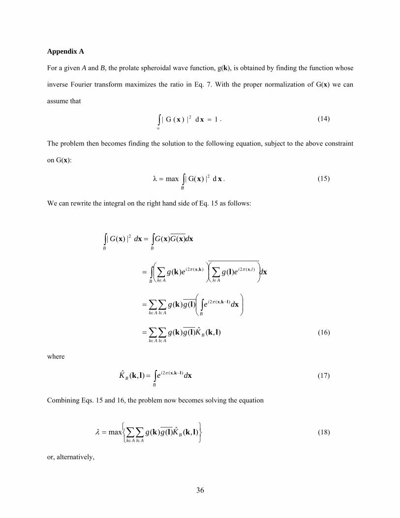
Appendix A
For a given A and B, the prolate spheroidal wave function, g(k), is obtained by finding the function whose
inverse Fourier transform maximizes the ratio in Eq. 7. With the proper normalization of G(x) we can
assume that
∫∞
= 1d|)(G| 2 xx . (14)
The problem then becomes finding the solution to the following equation, subject to the above constraint
on G(x):
∫=B
xx d|)G(|maxλ 2 . (15)
We can rewrite the integral on the right hand side of Eq. 15 as follows:
)()(|)(| 2 ∫∫ =BB
dGGdG xxxxx
∫ ∑∑ ⎟⎠
⎞⎜⎝
⎛⎟⎠
⎞⎜⎝
⎛=
∈∈B Al
li
Ak
i degeg xlk xkx ),(2),(2 )()( ππ
∑∑ ∫∈ ∈
−
⎟⎟⎠
⎞⎜⎜⎝
⎛=
Ak Al B
i degg xlk lkx ),(2)()( π
∑∑∈ ∈
=Ak Al
BKgg ),(ˆ)()( lklk (16)
where
∫ −=B
iB deK xlk lkx ),(2 ),(ˆ π (17)
Combining Eqs. 15 and 16, the problem now becomes solving the equation
⎭⎬⎫
⎩⎨⎧
= ∑∑∈ ∈Ak Al
BKgg ),(ˆ)()(max lklkλ (18)
or, alternatively,
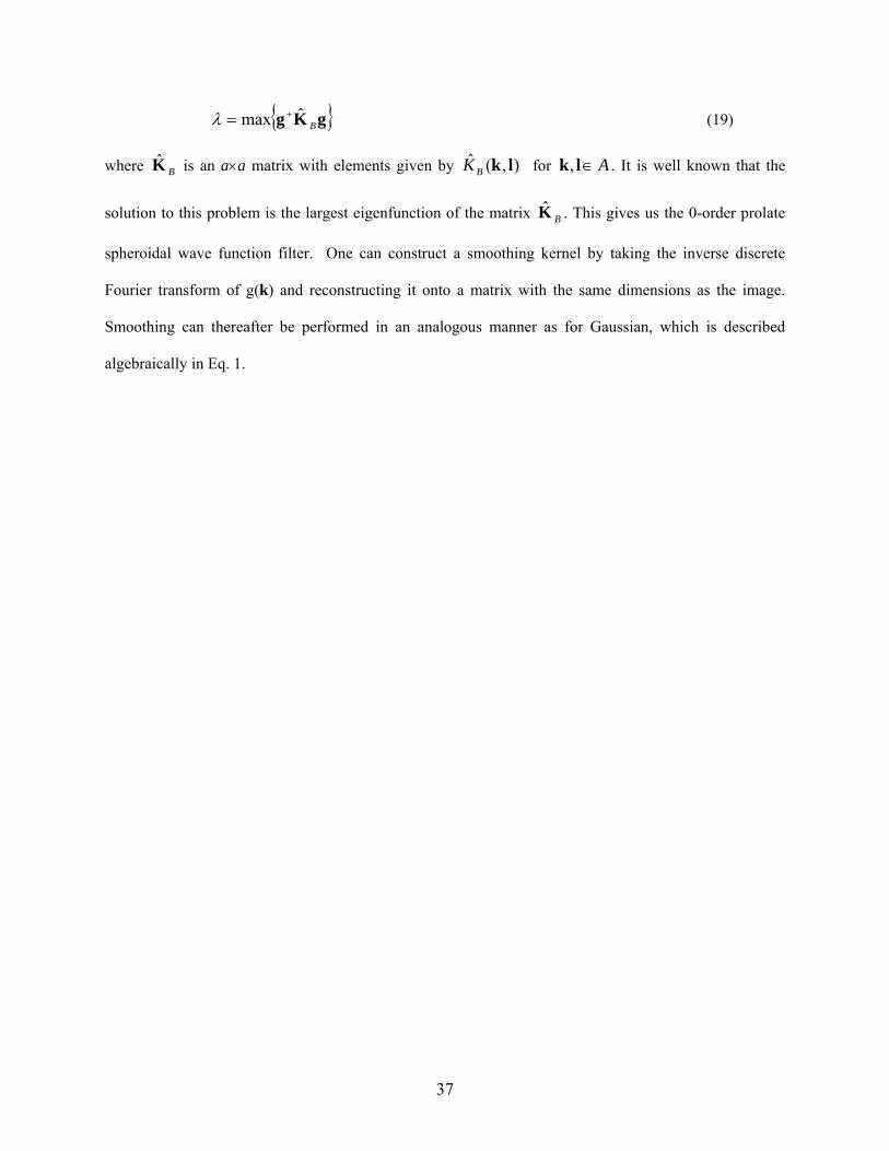
37
gKg Bˆmax +=λ (19)
where BK is an a×a matrix with elements given by ),(ˆ lkBK for A , ∈lk . It is well known that the
solution to this problem is the largest eigenfunction of the matrix BK . This gives us the 0-order prolate
spheroidal wave function filter. One can construct a smoothing kernel by taking the inverse discrete
Fourier transform of g(k) and reconstructing it onto a matrix with the same dimensions as the image.
Smoothing can thereafter be performed in an analogous manner as for Gaussian, which is described
algebraically in Eq. 1.
Recommended