SOME FACTORS AFFECTING SHORT-RUN
GROWTH RATES OF THE MONEY SUPPLY
Alfred Broaddus and Timothy Q. Cook
I.
introduction
Public interest in the monthly and weekly move- ments of the money supply’ has intensified since the
early 1970’s. One manifestation of this interest is
the extensive coverage of week-to-week and month- to-month changes in the money supply in the finan-
cial press. A second indication is the intense scrutiny of each new weekly or monthly money supply statistic
by financial market participants. Indeed, one of the
major current rituals in the markets is played out
late every Thursday afternoon as investors across the
nation hover around news wire machines awaiting the release of the latest weekly money supply figures.
The increased attentidn to short-run money supply
movements dates back to 1970 when the Federal Open Market Committee (FOMC), the Federal Re-
serve’s principal monetary policymaking body, began
to place greater weight on achieving specific longer- run growth rates for particular monetary aggregates.”
Under the current strategy of monetary policy,3 the FOMC periodically specifies desired longer-run growth rates (extending roughly a year ahead) for
certain monetary aggregates. These growth objec-
tives are publicly announced in quarterly testimony before one of the Congressional banking committees. At its monthly meetings the FOMC then reviews the state of the economy and compares the actual growth
of the aggregates with their desired long-run paths.
‘There are several concepts of the money supply. and statistical series corresponding to each of these “monetary aggregates” are published regularly in the Federcrl Reserve Bulletin. This article deals exclusively with the short-run behavior of MI, the most nar- rowly inclusive aggregate, which is comprised of (1) currency outside the Treasury, Federal Reserve Banks, and vaults of com- mercial banks; (2) demand deposits at commercial banks other than domestic interbank and U. S. Government deposits. less cash items in process of collection and Federal Reserve float; and (3) foreign demand balances at Federal Reserve Banks. MI is the aggregate most closely watched by financial market participants and the general public. Also, much of the short-run variability of the more broadly defined aggregates (all of which include i%) is due to the variability of ML
*This change in emphasis is evident in the evolving language of the FOMC’s directives to the Trading Desk at the Federal Reserve Bank of New York. Prior to 1970, the directives generally instructed the Desk to seek a desired condition in the money markets as indexed by interest rates or free reserves. Since 1970, in contrast, most directives have instructed the Desk to foster monw market and reserve supply conditions consistent with more rapid, slower, or unchanged growth of the monetary aggregates.
*See Lomhra and Torte C41 for a detailed description of the current strategy of monetary policy.
Based, on this review the FOMC specifies short-run
“tolerance ranges” for the growth rates of the aggre- gates over the two-month period covering the cur-
rent and following months. The aim in setting these
tolerance ranges is to define the near-term growth
rates most likely to be consistent with achieving the existing long-run growth objectives. Consistency in
this context, however, does not necessarily imply
equality. The short-run ranges can and often do deviate numerically from the long-run objective
either because the FOhilC is attempting to offset some unintended deviation in earlier months or be-
cause some temporary but foreseeable factor is es-
petted to affect short-run growth.
In any event, once the short-run tolerance ranges
are set, the FOhlC specifies a Federal funds rate range (normally from 50 to 100 basis points in
width) believed to be consistent with short-run monetary growth within the bounds of the tolerance
ranges. In this tactical framework, an emerging deviation of the actual two-month growth rates from
the specified tolerance ranges might lead the Federal
Reserve to alter the Federal funds rate (by increas- ing or decreasing the supply of nonborrowed reserves to member banks) in order to hold the growth rates
within the tolerance ranges. Finally-a point of
considerable importance-both the long-run mone- tary growth objectives and the two-month tolerance ranges are expressed in terms of seasonally adjusted
annual rates of growth. It should be evident from this description of the
Federal Reserve’s operating strategy that despite the longer-run time. horizon in which basic monetary
growth goals are cast, the procedure by its nature
tends to focus day-to-day attention on short-run monetary movements. First, from the standpoint of
the Federal Reserve, the key tactical operating speci- fication is the two-month tolerance range. Setting an
appropriate range requires close attention to the numerous factors affecting current weekly and
monthly growth rates. Further, incoming weekly and monthly data must be continuously tracked and evaluated against the criteria established by the toIer-
ante ranges. Second, the procedure naturally stimu-
2 ECONOMIC REVIEW, NOVEMBER/DECEMBER 1977
lntes financial market interest in the short-run be- havior of the aggregates. Given this procedure, these nlovements strongly influence market expectations
regarding the likelihood that the Federal Reserve \vill seek a change in the Feder;~l funds rate that will
in turn influence tlie lx-ices and yields of other finan-
cial instruments. ;is a I-esult. considerable resources
\vitliin the markets are no\v devoted to “watching” hot11 the Federal Resell-e 2nd the money supply.
Tlie major difficult). that arises in this institutional
fr:liiie\vork is that short-run monetary data, even
after seasonal adjustment. xe highly volatile. It is therefore difficult to project short-run movements,
even for the immediate future, and equally difficult
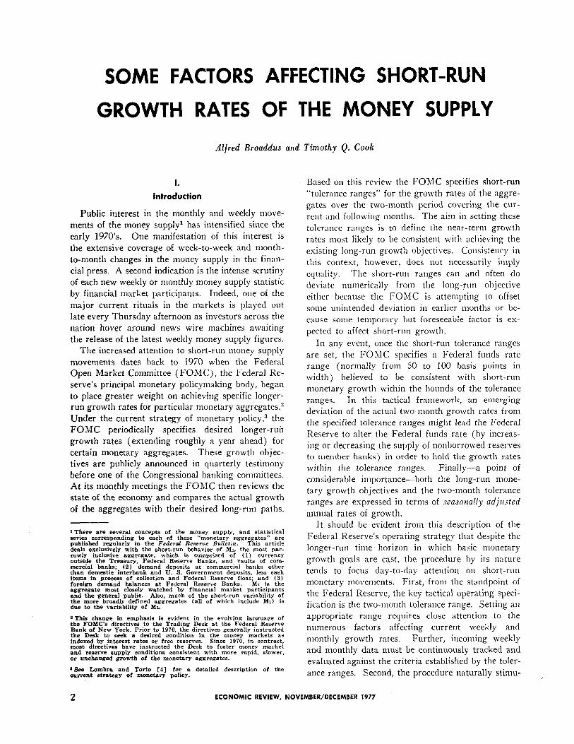
to evaluate incoming data. Cliart 1 illustrates this
volatility. It conilx~res tlie originally published or “l)reliminar~“~ seasonally adjusted one- and two-
month ;\I1 grokvth rates (at annual rates) in 1975
and 1976 \vith the full year g-ro\vth rates during the surrounding 12-month period. Table I provides a
‘As evidence of this expectational impact. the corwlation coeffi- cient between the chanse in MI announced Thursday and the char.re in the three-month Treasury bill rate the followins day was 26 over the 52 weeks of 19i6, which is statistically significant at the 5 percent level.
z Throughout this article, “preliminary” refers to the MI statistic first published covering a particular period. “Final” refers to the most recently revised statistic for a period. The emphasis will be on the preliminary data since it is the preliminary data to which both the Federal Keserve and the financial markets react.
further illustration. It shows the standard deviations of the annualized preliminary one- and two-month
l\iI, growth rates in each of the last ten years. The average standard deviation is 5.5 percentage points for the one-month growth rate and 3.8 percentage
points for the two-month growth rate. Strikingly, the standard deviation of the one-month growth rates actually exceeds the average monthly growth rate in a
number of years. This volatility of short-run growth rates relative to trend would not constitute a serious
problem if it were possible to distinguish, on a cur- rent basis, between transitory changes in money
growth and more permanent changes related to basic
economic developments. Unfortunately, making such distinctions is an extremely difficult task. Conse- quently, the possibility always exists that the short-
run behavior of the monetary aggregates might mis- lead either the Federal Reserve or market partici-
pants observing and trying to anticipate Federal
Reserve actions.
The purpose of this article is to provide some in-
sights into the difficulties inherent in interpreting the
short-run behavior of the seasonally adjusted mone-
tary aggregates and to provide a framework for analyzing certain kinds of short-run swings. The
article lvill focus on variations caused by factors other than changes in basic underlying conditions in
1 I Chartl~“, I, d_ *
PRELIMINARY SHORT-RUN Ml GROWTH RATES COMPARED TO LONGER-RUN GROWTH RATES .’ *
Percqt (SAAR) I: A _ i c
18 t
1 1’6.
----- 1 -Month
- P-Month
.---a l-Year
FEDERAL RESERVE BANK OF RICHMOND
Table I
STANDARD DEVIATIONS AND MEANS OF
PRELIMINARY SHORT-RUN Ml GROWTH RATES
(SAAR)
1967 1968 1969
1970
1971 1972
1973
1974
1975
1976 5.2 5.6
Average 5.5
Source: Federal Reserve Bulletin.
One-Month Growth Rates Two-Month Growth Rates
Standard standard Deviation Mean Deviation Mean ~ -
6.7 6.6 4.0 6.6 4.9 6.5 3.7 6.1 3.6 1.9 2.1 2.1 6.0 4.5 3.5 4.2 6.5 6.1 5.5 6.3 4.9 8.0 3.2 7.5 5.1 5.6 4.1 5.4 4.5 4.9 3.0 5.1 7.7 4.7 5.4 4.7
3.3 5.2
3.8
the economy. As indicated in the sections that follow,
these noneconomic factors are responsible for a sub stantial portion of the observed illouth-to-moIltl~ and
week-to-week variations in monetary growth rates. The next section of the article describes in general terms the various kinds of noneconomic factors that
produce short-run movements in the preliminary XI, data. Special attention is devoted to movements that
result from the nature of the procedures currently
used to seasonally adjust the data. The third section illustrates some of the points made in the second
section with specific examples of factors affecting monthly M1 growth rates in recent years. The
fourth section provides further illustrations with
reference to the weekly M1 statistics. The final
section contains a brief summary of the article and
presents a few conclusions.
II.
Some Factors Affecting Short-Run Movements in
Money Growth Rates: A General Description
This section will discuss in general terms some of the noneconomic factors that produce variations in
seasonally adjusted short-run Ml growth rates. Ob- served growth rates are no doubt related in some
way to changes in economic conditions. But factors
totally unrelated to current business conditions can cause significant variations in these growth rates.
Special nonrecurring events can have an important effect on demand deposit balances in some cases over
periods of several weeks. Moreover, seasonal adjust-
ment techniques, despite notable improvemer, ts in recent ).ears. are far from perfect. Over long periods,
variations in the M1 data related to both special
events and seasonal adjustment problems should
wash out. But factors such as these produce sharp
fluctuations in short-run growth rates.
It will be useful in organizing the discussion to
distinguish two classes of variations : ( 1) movements that result from shortcomings in the method cur-
rently used to seasonally adjust the data and (2)
irregular variations due to special nonrecurring events. Each of these two categories of factors will
be addressed in turn. The focus throughout this section is primarily on the monthly data.
Variations Due to Deficiencies in the Seasonal
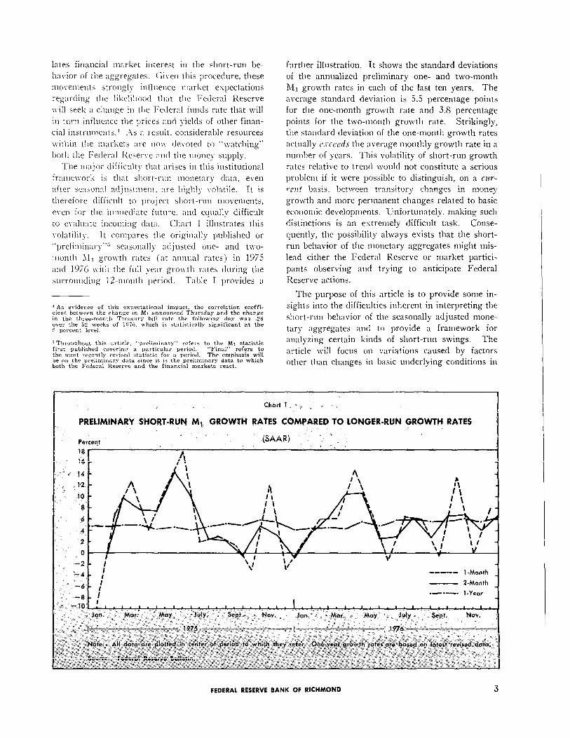
Adjustment Procedures Chart 2 shows the an-
nualized monthly growth rates of ~of seasonally ad-
justed M1 in 1973, 1975, and 1976. It is evident from the chart that these growth rates are extremely
variable, ranging from over 3070 to under -3070, and that they are dominated by recurring seasonal
Inovenients. A glance at the chart suggests two of
the major forces underlyin, 0 this seasonal movement :
tax dates--April, in particular, \vheii individuals ac-
cumulate balances to pay income tnses-and the iti- creased business activity during the Christnlas season.
As described in Box I on 11. 5, the M1 data are
seasondly adjusted with seasonal factors computed I)): the I<ureau of the Census’ S-1 1 Variant of the
Census Metllotl I1 Seasonal Adjustment Program (referi-etl to below as X-1 1) Judgmental modifica- tions are then made by the Federal Reserve staff in
\ h~~“jl e
,* i- : ” ;&g12” 3,; “- pi s” ,‘
NOT SEASbNALLY “ADJUSTED MONTHLY M, GROWTH RATES ~
4 ECONOMIC REVIEW, NOVEMBER/DECEMBER 1977
Box I
SEASONAL ADJUSTMENT OF THE MONEY SUPPLY: THE PROBLEM OF MOVING SEASONALS
As indicated in the text, money supply data are seasonally adjusted I)y the Federal Reserve staff using the Census Bureau’s S-11 Variant of the Census Method I I seasonal adjustment model, re- ferred to belo\v simply as X-11. ITsing unadjusted data for a period of years, this ~notlcl generates a seasonal adjustment factor for each entry in the series: for example, for each individual month in a monthly series of money stock data. In deter- mining the final seasonal adjustment factors actu- ally cmploycd in developing the published season- ally adjusted money supply series, the staff may alter the adjustment factors derived from the model where the staff’s knoxvledge of special circum- stances affecting the X-11 factors suggests such alterations are in order. What follows is a brief description of some of the problems encountered in applying X-11 to money supply data. (For a
detailed description and analysis of Federal Reserve procedures used in seasonally adjusting the money supply, see the accompanying article I)y Lawler.)
Like most conventional seasonal adjustment pro- cedures, X-11 assumes tllat the lcvcl of an unad- justed data series (call it Munad in the case of monthly money supply data) at any point in time reflects the combined influence of four underlying determinants: long-term trend movements (T), cyclical movements (C), regularly recurring sea- sonal movements (S), and irregular movements (I). The version of X-11 used the Federal serve assumes four determinants related to another in multiplicative, i.e., fashion:
hl = T c X 2; I.
this general one can two alternative under xvhich influences might the unadjusted supply data: a condition the pattern seasonal influences constant from to year
(2) a where the changes from year to next. 111 iirbt case, multi-
ljlicativc proportionate inlpact seasonal influ- on tlie data is hame for
particular calendar (say, January) all of years covered the series. these condi-
any computed of seasonal factors, S, January, February, respectively, should constant over full span years covered the series. the second the pro-
impact of influences during given calendar changes over To re-
these changes seasonal adjustment for each month should, general,
change out year the next. has alternative modes designed
deal with of these sets of As applied any set monthly data, X-11 model essentially a average sea-
adjustment procedure. means that seasonal adjustment are derived develop- ing of (1) unadjusted data individual months example, June in the to
(2) average of months data on that Such a is calculated each individual in the The seasonal justment factor each individual is then
by averaging ratio for month with ratios for corresponding calendar
in other The two modes mentioned enter the as follows. the pattern seasonal influences the data believed to stable over a single adjustment factor derived for of the calendar months an average all of the ratios for that calendar month over the full series. If the pattern is believed to be changing over time, a moving average of such ratios, covering a more abbreviated time span, is used to compute a distinct adjustment factor for each individual month in the series.
For the reasons given in the text, it is clear that the seasonal pattern of the unadjusted monthly money supply series is not constant but changes over time. Therefore the version of X-11 used to adjust the money supply data derives seasonal ad- justment factors for each individual month in the series from a weighted 7-term moving average of the ratios in the corresponding calendar months of surrounding years. Where a month is in one of the terminal years of the series, the span of the moving average is reduced since data for a full centered 7-term moving average are not available. For example, the presently published adjustment factor for January 1973 (an example of what is called “final” data in the text) is derived from a weighted average of the January ratios for the years 1970- 1976, inclusive. The presently published factor for January 1976 is derived from the four year period 1973-1976, inclusive.
It is important to note that under this procedure, the factors used to seasonally adjust incoming data during the current year-the all important “prelimi- nary” data to which both the Federal Reserve and the markets react-are derived from ratios of pre- ceding years and do not directly reflect any changes in seasonal patterns in the current year.* For ex- ample, the seasonal factor used to adjust the Janu- ary 1973 figure when the figure was initially re- leased in early February 1973 was derived from the January ratios for the years 1969-1972, inclusive. Therefore, if the seasonal pattern is in fact chang- ing in the current year, it is particularly likely that the procedure will distort the preliminary, i.e., current, data. Ironically, this is precisely the data of greatest importance to Fed policymakers and the markets. The discussion in the text describes some of the distortions that arise and shows that these distortions are a source of seasonal movement in the seasonally adjusted money supply data.
* Strictly speaking the weights attached to these preceding year ratios might implicitly cause the procedure to anticipate current year changes to a small extent.
FEDERAL RESERVE BANK OF RICHMOND 5
an effort to compensate for some of X-11’s deficien-
cies.” As indicated in the ljox, the purpose of se;l- sonally adjusting lhf , is to eliminate the impact of seasonal forces, leaving only trend, cycle and irregu-
lar movements. In practice, however, the influence of seasonal forces is often not eliminated from tile preliminary seasonally adjusted M, data. A majoi reason for this residual seasonality is that X-l 1 neces- sarily relies solely on past data in calculating pre- liminary seasonal adjustment factors and therefore cannot take full account of changes in seasonal l)e- havior currently in progress, despite the program’s
allowance for “moving” seasonnls described in tile Box.
A variety of developments can change the relative
impact of seasonal events on the money supply in a
particular month. First, there are changes in the
tiutling of seasonal events. For example, in 1955 the
final day for the payment of nonwithheld individual
Federal income taxes was permanently shifted from
March 15 to April 15. A contrasting example is the
continuously shifting calendar position of the Easter
holiday. Second, the relative magnitude of sctrsonnl
force can change. The aggregate amom7t of individ-
ual or corporate taxes paid in a given month relative
to the level of the money supply, for instance, might
deviate from the usual norm. This deviation might
be due either to a change in the total tax liability
relative to M1 or to a change in the distribution of
payments over the various periodic tax payment
dates within the year. Third, the VUWULCY in which
households and bzrsincss firms wanage their UIOIIE~
balances during periods characterized by recurring
seasonal events can change. For example, improved
corporate cash management practices have probabl)
compressed the necessary lead-time for the accumLi-
lation of cash balances prior to scheduled tax pay-
ments. Finally, neza, seasonal events appear from
time to time. In late 1972, for instance, the Federal
government initiated sizable revenue-sharing pay-
ments at the beginning of each quarter.
The impact of these several changing seasonal
forces on short-run seasonally adjusted Ml growth
rates is likely to vary, depending particularly on (1)
whether the change is permanent or temporary and
(2) if permanent, whether the change occurs gradu-
0 See the accompanying article by Lawler for a description of these judgmental modifications. In making these modifications the staff faces many of the same difficulties anticipating changes in seasonal patterns encountered by the X-11 proaram itself. For this reason it is not clear that the modifications significantly improve the preliminary data. In any case, this article does not attempt to evaluate these modifications.
ally over :I period of years or abruptly. Moreover, tile inil)act of tliese changes on the preliminary (i.e..
first l)ul)lislietl) adjusted data for a particular month is likely to differ from tlleir impact on the final
revised tlata for the month. The folloning para- gr~plis will el:J)ornte these points.
Consider first the final data. As indicated in the
hs, S-l 1 uses a seven-year weighted nioving aver-
age of data centered on a given year in deriving final
seasonally adjusted data for that year.’ For this
reason, the program is especially well suited to ac-
commodating, after the fact, gmdrta! changes in
underlying seasonal patterns since the centered,
seven-year nioving average by its very construction
should capture such changes. On the other hand,
the program is not particularly well suited to dealing
with permanent changes that occur abruptly. As an
example, assume that a lasting change in some sen-
sonal event affecting M1 occurred abruptly in 1973.
Here, even the final adjusted monthly data for 1973
might not adequately capture the change since the
final data, derived from the seven-year centered
moving average, would be based partly on experience
during the years 1970, 1971, and 1972-all years
preceding the change.
Consider next the more significant preliminary
data. Kegardless of whether a permanent change in
underlying seasonal forces occurs gradually or
abruptly, the preliminary adjusted growth rates are
likely to be distorted in the seiise that they will
probably differ systematically from revised data pub
lished later. The reason for these distortions is that
S-l 1 derives preliminary adjustment factors from
actual data for years preceding the year in question.
(See Box.) Consequently, the preliminary factors
fail to capture the full effects of changes in under-
lying seasonal behavior. Such distortions are ob-
viously significant since it is the preliminary adjusted
Ml data that condition current monetary policy and
the behavior of the financial markets.
A couple of hypothetical examples might help to
clarify the nature of these distortions. Suppose that
begimiing in 19S0, the unadjusted growth rates of
hII in the month of October began to display a
g~~drtnl but persistent decline due, perhaps, to a
7 The term “final” may be slightly misleading in that money susplr data is always subject to further revision. The term is used hers, to refer to revised adjusted data available beginnina in the fourth year following the year to which it applies. Such data is seasonally adjusted using adjustment factors that are derived from actual data for the full seven-year period covered by the seven-term movins average in the X-11 program.
6 ECONOMIC REVIEW, NOVEMBER/DECEMBER 1977
decline in the relative volume of business sales in
that month. Suppose further that this trend per- sisted through the year 1990. Under these circum- stances, the X-11 seasonal adjustment factor used to
compute the prelinlinary seasonally adjusted growth rate in, say, October 19S5 would reflect the move- ment in M, in the years 19Sl-19%. Consequently,
this preliminary factor would be biased upward and
the preliminary seasonally adjusted growth rate
\voultl l)e understated.X In subsequent years the
October 19% gro\vth rate \vould be revised upward. The preliminary gro\vth rates for Octoijer in ensuing J’ears, ho\vever. would continue to differ systemati-
cally from revised gro\vth rates as long as the trend
continued.
Consider next an ab,-lip1 future change in a sea-
sonal event such as, for instance. a hypothetical change in the deadline for iiidi~idual Federal income t;ls l~:tyinents from April 15 to May 15. Suppose that such :I cllange Ivent into effect in 19S6. In that
case, beg-inning in 19SG the unadjusted growth of MI in April would be low \\hile not seasonally adjusted gro\vth in Slay would be high relative to the pattern
in earlier years. Here, the preliminary seasonal ad- jListment factors for April and Llay 19SG would be I)asetl on i\l, I)ehavior over tlie 19S2-19S5 period. Consequently, the preliniinnry adjusted growth rate
for April 19SG would proba1~1y I)e unusually low,
\\-bile the R’lny 1924 growth rate \vould be signifi- cantly inflated. In the absence of further changes. however, the problem would tend to disappear by 1990 since by that year all of the data used in de-
riving the preliminary April and May adjustment
factors would reflect the 19SG tax date change.
Beyond the more durable seasonal developments
discussed to this point, temporary changes can also
affect short-run seasonally adjusted monetary growth
rates. As ;L final ex;unple, suppose that Federal tax
payments by individuals were unusually large relative
to the level of Ml in April 19S3, but that in 19S3
and subsequent years, the payments fell back to more normal levels. In this case the preliminary seasonal adjustment factor for April 19S3, which would be based on 1979-1932 experience, would be low relative
to the level of the tax payments. Hence, in the
absence of some other ulwsual event tending to de- press growth, the preliminary seasonally adjusted RiIl
growth rate for April 19S3 would be relatively high. Further, the final revised data for this month would
‘The X-11 prozram does contain an adjustment designed to correct partially for trend changes in seasonal behavior. See r7, p, 161. As long as the chanaes continue nt roughly the same pace. however. the correction will be only partial, and the bias discussed in the text will persist.
also show a relatively high growth rate under these circumstances.
It should be clear from this discussion that the
procedure presently used to seasonally adjust mone- tary data is itself an important potential source of short-run variations in adjusted monetary growth rates.
Irregular Variations In addition to the effects
of changing seasonal patterns working through
the seasonal adjustment procedures, short-run M,
growth rates are also strongly influenced at times by
irregular, nonrecurring events. In contrast to sea-
sonal movements no effort is made to remove such
irregular movements from the adjusted Ml data.
While the events underlying these movements are
not always fully understood, in many instances the
explanation is straightforward. One of the best
examples of a large irregular movement in recent
years was the bulge in Ml in May and June 1975
following the $9 billion disbursement of tax rebates
and supplemental social security payments by the
Treasury to the public.!’
It should be noted parenthetically that the dis- tinction between ( 1) irregular movements and (2) the movements discussed above reflecting temporary
changes in seasonal forces is not always clear. In
the preceding section the example used to illustrate
temporary seasonal forces was unusually large indi- vidual tax payments in one year. Some analysts
might prefer to regard such an occurrence as an irregular event. The criterion adopted in this article is that events that recur with some definite periodic-
ity are seasonal in nature, while other events are
irregular. Whatever the distinction in principle, in
practice both categories of events are likely to pro- duce short-run movements in the seasonally adjusted M1 data, As indicated above, the X-11 program is unlikely to remove the effects of temporary changes
in seasonal patterns from the seasonally adjusted data, and irregular movements are left in the adjusted
series by design.‘”
The following section illustrates the foregoing dis- cussion with specific empirical examples from recent
experience.
!‘See Breimyer and Wenninaer [z] for empirical evidence on the impact of the rebntes on seasonally adjusted monthly Ml growth rates in 1975.
‘OIt might be added that both irregular movements and movements due to temporary changes in seasonal forces can present additional problems if they are mistakenly treated as permanent changes in seasonal patterns by the X-11 pro!zram. In addition. computed seasonal adjustment factors might be distorted by cyclical develop- ments. See Lawler 13, p. 241 and Poole and Lieberman [6, pp. 325-3341.
FEDERAL RESERVE BANK OF RICHMOND 7
III.
Factors Affecting Short-Run Money Growth Rates:
Some Empirical Examples
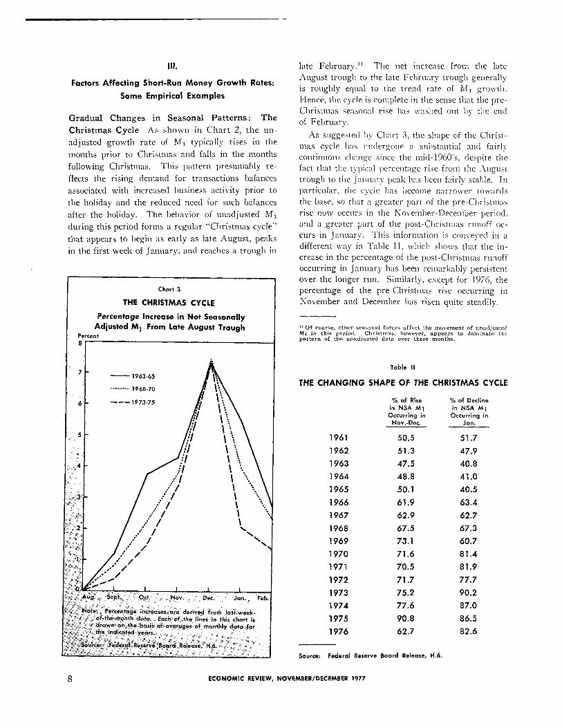
Gradual Changes in Seasonal Patterns: The
Christmas Cycle As shown in Chart 2, the un-
adjusted growth rate of M1 typically rises in the
months prior to Christmas and falls in the months
following Christmas. This pattern presumably re-
flects the rising demand for transactions balances
associated with increased business activity prior to
the holiday and the reduced need for such balances
after the holiday. The behavior of unadjusted M1
during this period forms a regular “Christmas cycle”
that appears to begin as early as late August, peaks
in the first week of January, and reaches a trough in
Chart 3
THE CHRISTMAS CYCLE
Percentage increase in Not Seasonally Adjusted M1 From late August Trough
Percent
- 1963-65
- . ..-..... ,96*.,0
--- 1973-75
late February.” The net increase from the late
August trough to the late February trough generalI> is roughly equal to the trend rate of iLlI1 growtll.
Hence, the cycle is complete in the sense that the pre- Christmas seasonal rise has nashed out by the end
of February.
As suggested by Chart 3, the shape of the Christ- mas cycle has undergone :I sulMaiitia1 and fairI> continuous change since the mid- 1960’s. despite the fact that the typical percentage rise from the August
trough to the January peak has been fairly stable. In particular, the c).cle has become narrower to\vartls
the base, so that ;I greater part of the pre-Christmas rise now occurs in the November-December period, and a greater part of the post-Christmas runoff oc- curs in January. This information is convey-ed in a
different way in Table II, which shows that the in- crease in the percentage of the post-Christmas runoff
occurring in January has been remarkably persistent over the longer run. Similarly, except for 197G, the percentage of the pre-Christmas rise occurring in
November and December has risen quite steadily.
1’ Of course, other seasonal forces affect the movement of unadjusted MI in this period. Christmas, however, appears to dominate the pattern of the unadjusted data over these months.
Table II
THE CHANGING SHAPE OF THE CHRISTMAS CYCLE
% of Rise % of Decline in NSA ,441 in NSA Ml
Occurring in Occurring in Nov.-Dec. Jan.
1961 50.5
1962 51.3
1963 47.5
1964 48.8
1965 50.1
1966 61.9
1967 62.9
1968 67.5
1969 73.1
1970 71.6
1971 70.5
1972 71.7
1973 75.2
1974 77.6
1975 90.8
1976 62.7
SOUVX Federal Reserve Board Release, H.6.
51.7
47.9
40.8
41.0
40.5
63.4
62.7
67.3
60.7
81.4
81.9
77.7
90.2
87.0
86.5
82.6
8 ECONOMIC REVIEW, NOVEMBER/DECEMBER 1977
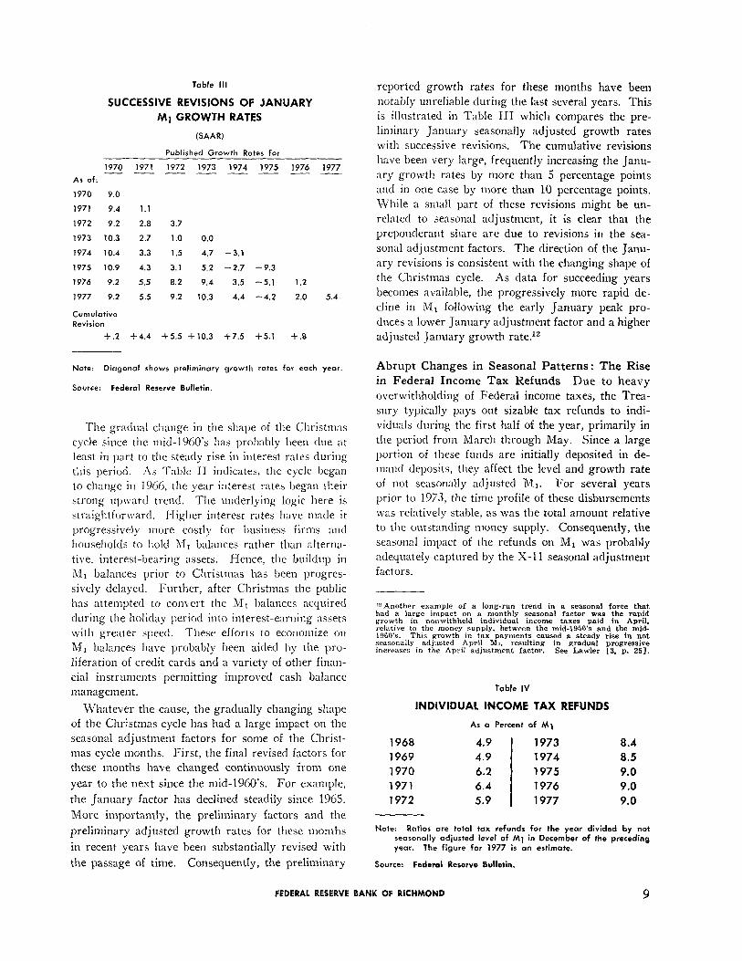
Table III
SUCCESSIVE REVISIONS OF JANUARY
Ml GROWTH RATES
(SAAR)
Published Growth Rates for
1970 1971 1972 1973 1974 1975 1976 1977 --I_----- As of:
1970 9.0
1971 9.4 1.1
1972 9.2 2.8 3.7
1973 10.3 2.7 1 .o 0.0
1974 10.4 3.3 1.5 4.7 -3.1
1975 10.9 4.3 3.1 5.2 -2.7 -9.3
1976 9.2 5.5 8.2 9.4 3.5 -5.1 1.2
1977 9.2 5.5 9.2 10.3 4.4 -4.2 2.0 5.4
Cumulative Revision
+.2 +4.4 +5.5 +10.3 +7.5 +5.1 + .a
Note: Diagonal shows preliminary growth rates for each yeor.
Source: Federal Reserve Bulletin.
The gradual change in the shape of the Christmas cycle since the mid-1960’s has probably been due at least in part to the steady rise in interest rates during
this period. As Table 11 indicates, the cycle began to change in 1966, the year interest rates began their strong upward trend. The underlying logic here is straightforward. Higher interest rates have made it progressively more costly for business firms and households to hold Mt balances rather than alrertia-
tive, interest-bearing assets. Hence, the buildup in Mt balances prior to Christmas has been progres-
sively delayed. Further, after Christmas the public
has attempted to convert the Mt balances acquired
during the holiday period into interest-earning assets with greater speed. These efforts to economize on
M1 balances have probably been aided by the pro-
liferation of credit cards and a variety of other finan- cial instruments permitting improved cash balance
management.
Whatever the cause, the gradually changing shape of the Christmas cycle has had a large impact on the
seasonal adjustment factors for some of the Christ- mas cycle months. First, the final revised factors for these months have changed continuously from one
year to the next since the mid-1960’s. For example,
the January factor has declined steadily since 1965.
More importantly, the preliminary factors and the
preliminary adjusted growth rates for these months
in recent years have been substantially revised with
the passage of time. Consequently, the preliminary
reported growth rates for these months have been nofably unreliable during the last several years. This is illustrated in Table III which compares the pre-
liminary January seasonally adjusted growth rates with successive revisions. The cumulative revisions
have been very large, frequently increasing the Janu- ary growth rates by more than 5 percentage points and in one case by more than 10 percentage points.
While a small part of these revisions might be un- related to seasonal adjustment, it is clear that the
preponderant share are due to revisions in the sea- sonal adjustment factors. The direction of the Janu- ary revisions is consistent with the changing shape of
the Christtnas cycle. As data for succeeding years becomes available, the progressively more rapid de-
cline in M1 following the early January peak pro-
duces a lower January adjustment factor and a higher adjusted January growth rate.l’
Abrupt Changes in Seasonal Patterns: The Rise
in Federal Income Tax Refunds Due to heavy
overwithholding of Federal income taxes, the Trea- sury typically pays out sizable tax refunds to indi-
viduals during the first half of the year, primarily in the period from March through May. Since a large
portion of these funds are initially deposited in de- mand deposits, they affect the level and growth rate of not seasonally adjusted Ml. For several years prior to 1973, the time profile of these disbursements
was relatively stable, as was the total amount relative to the outstanding money supply. Consequently, the
seasonal impact of the refunds on Mt was probably adequately captured by the X-l 1 seasonal adjustment
factors.
“Another example of a long-run trend in a seasonal force that had a large impact on a monthly seasonal factor was the rapid growth in nonwithheld individual income taxes paid in April. relative to the money supply, between the mid-1950’s and the mid- 1960’s. This growth in tax payments caused a steady rise in not seasonallr adjusted April M1, resulting in gradual progressive increases in the April adjustment factor. See Lawler 13. p. 261.
Table IV
INDIVIDUAL INCOME TAX REFUNDS
As Q Percent of Ml
1968 4.9 1973 8.4
1969 4.9 1974 8.5 1970 6.2 1975 9.0 1971 6.4 1976 9.0 1972 5.9 1977 9.0
Note: Ratios we total tax refunds for the year divided by not seasonally adjusted level of Ml in December of the preceding year. The figure for 1977 is an estimate.
Source: Federal Reserve Bulletin.
FEDERAL RESERVE BANK OF RICHMOND 9
.-.-.- 1970- 72
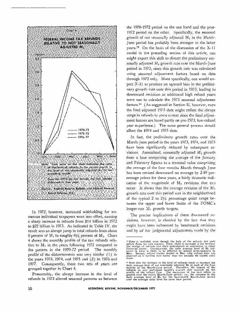
In 1972, however, increased withholding for nu- merous individual taxpayers went into effect, causing a sharp increase in refunds from $14 billion in 1972
to $22 billion in 1973. As indicated in Table IV, the result was an abrupt jump in total refunds from about
6 percent of M, to roughly 8% percent of M,. Chart 4 shows the monthly profile of the tax refunds rela-
tive to MI in the years following 1972 compared to the pattern in the 1970-72 period. The monthly
profile of the disbursements was very similar (1) in
the years 1973, 1974, and 1975 and (2) in 1976 and
1977. Consequently, these two sets of years are grouped together in Chart 4.
Presumably, the abrupt increase in the level of refunds in 1973 altered seasonal patterns as between
the 1970-1972 period on the one hand and the post-
1972 period on the other. Specifically, the seasonal
growth of not seasonally adjusted Ml in the March-
June period has probably been stronger in the latter
years.13 On the basis of the discussion of the X-11
model in the preceding section of this article, one
might expect this shift to distort the preliminary sea-
sonally adjusted M, growth rate over the March-June
period in 1973, since this growth rate was calculated
using seasonal adjustment factors based on data
through 1972 only. More specifically, one would ex-
pect X-11 to produce an upward bias in the prelimi-
nary growth rate over this period in 1973, leading to
downward revisions as additional high refund years
were use to calculate the 1973 seasonal adjustment
factors.14 (As suggested in Section II, however, even
the final adjusted 1973 data might reflect the abrupt
surge in refunds to some extent since the final adjust-
ment factors are based partly on pre-1973, low-refund
year experience.) The same general process should
affect the 1974 and 1975 data.
In fact, the preliminary growth rates over the
March-June period in the years 1973, 1974, and 1975
have been significantly reduced by subsequent re-.
visions. Annualized, seasonally adjusted M, growth
from a base comprising the average of the Januar)
and February figures to a terminal value comprising
the average of the four months March through June
has been revised downward on average by 2.49 per-
centage points for these years, a fairly dramatic indi-
cation of the magnitude of &I1 revisions that ca!n
occur. It shows that the average revision of the Ml
growth rate over this period was in the neighborhood
of the typical 2 to 2yz percentage point range be-
tween the upper and lower limits of the FOMC’s
longer-run Ml growth targets.
The precise implications of these downward re-
visions, however, is clouded by the fact that they
might have been influenced by benchmark revisions
and by ad lzoc judgmental adjustments made by the
1J June is included, even thouph the bulk of the refunds are paid before June, for two reasons. First, there is normally a lag between the receipt of refunds and their expenditure or conversion to Other financial assets. Consequently, the daily average level of MI bal- ances in June is likely to be affected by refund disbursements in May. Second, refund checks mailed in May (the refund data are reported on a mailing date basis) may not actually be cashed until JUWZ.
14 Note that the increase in the level of refunds tends to increase the daily average level of not seasonally adjusted Ml in each of the fsxxr months of the March-June period. Therefore, the impact of the refunds on any individual month’s growth rate depends on the profile of the refund flow. The discussion in the text refers to growth over the entire March-June period: i.e., the increase in the daily average level of Mt for the four-month March-June pwiod over the average daily level for some base period.
10 ECONOMIC REVIEW, NOVEMBER/DECEMBER 1977
staff of the Board of Governors as well as by changes in the underlying zX-l 1 seasonal adjustment factors. In order to abstract from these other factors, com- parable growth rates were calculated using the factors generated by the X-l 1 model without any modifica-
tion. First, unmodified X-l 1 seasonal adjustment
factors were calculated using data through 1972, and
these factors were then used to develop a “prelimi-
nary” growth rate for the March-June 1973 period
(over a January-February 1973 base). Preliminary
March-June growth rates for 1974 and 1975 were
derived in a similar manner. These preliminary
growth rates were then compared to “final” growth
rates for the same periods derived from unmodified
X-11 factors computed using data through 1976.
The implied revisions are -1.70 percentage points
in 1973, -1.56 percentage points in 1974, and -1.06
percentage points in 1975-an average revision of
-1.44 percentage points. This analysis suggests that
successive changes in the underlying X-11 factors
contributed heavily to the revision in the published
M1 data summarized in the preceding paragraph.‘”
To this point the discussion has centered on the
impact of the increased tax refunds on the prelimi-
nary seasonally adjusted M, data over the March-
June period. More broadly, there is evidence that the
increased refunds in conjunction with the X-l 1 model
generally biased the preliminary seasonally adjusted
growth rates upward in the second quarter and down-
ward in the third quarter in 1973 and subsequent
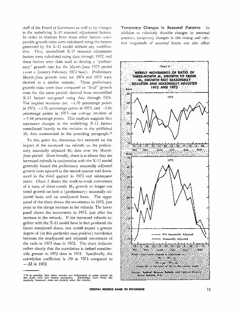
years. Chart 5 shows the week-to-week movements
of a ratio of three-month Ml growth to longer-run
trend growth on both a (preliminary) seasonally ad-
justed basis and an unadjusted basis. The upper
panel of the chart shows the movements in 1972, just
prior to the abrupt increase in the refunds. The lower
panel shows the movements in 1973, just after the
increase in the refunds. If the increased refunds to-
gether with the X-l 1 model have in fact produced the
biases mentioned above, one would expect a greater
degree of (in this particular case positive) correlation
between the unadjusted and adjusted movements of
the ratio in 1973 than in 1972. The chart indicates
rather clearly that the correlation is indeed consider-
ably greater in 1973 than in 1972. Specifically, the
correlation coefficient is .70 in 1973 compared to
-.22 in 1972.
‘6It is possible that these results are influenced to some extent by the June 1975 tax rebate payments. Excluding June from the analysis. however, does not greatly alter the results.
Temporary Changes in Seasonal Patterns In
addition to relatively durable changes in seasonal
patterns, temporary changes in the timing and rela-
tive magnitude of seasonal forces can also affect
FEDERAL RESERVE BANK OF RICHMOND 11
seasonally adjusted M1 growth rates.‘” Although
X-11 attempts to take account of lasting changes in the profile of seasonal forces influencing M, through
the construction of moving adjustment factors, the model is simply not designed to deal effectively with temporary changes in these forces. Basically, the model treats such changes as though they were ir-
regular movements in the not seasonally adjusted data. Consequently, most of their impact is probably passed on to the seasonally adjusted data. For example, since there is a positive relationship be- tween the relative magnitude of April tax payments
and the unadjusted lMl growth rate in April, unusu-
ally large April tax payments in a given year prob- ably tend to inflate the seasonally adjusted April M1
growth rate in that year.
A somewhat more esoteric example involves the timing of April tax collections by the Treasury.
Individuals generally pay nonwithheld income taxes by check. Many of these checks are mailed close to the April 15 deadline. Individuals typically accumu- late the balances needed to cover these checks at the
time they are mailed, but the Treasury often takes
two or three weeks to process the checks. Because of
the huge sums involved, even a small variation in processing time can significantly affect average daily M1 balances in April and seasonally adjusted April
M, growth rates.‘?
A final example is a recent change in the proce- dures surrounding monthly social security retirement
and survivors benefit (SSA) disbursements. Prior to mid-1976 all of these disbursements were made bj check. The checks were usually posted so that they would reach .their recipients on the third of the month. When the third fell on a Saturday, payment was made on that day even though some financial
institutions are closed on Saturdays. If the third fell on a Sunday, payment was made on the preceding
Saturday. In mid-1976 this schedule was changed
in conjunction with the introduction of facilities per- mitting the direct deposit of some of these clisburse-
ments through electronic media. Specifically, pay-
ments are now made on the preceding Friday when the third falls on either a Saturday or a Sunday.‘8
Since a sizable portion of the disbursements are con- verted into -R/I1 balances, these changes in payment
In As indicated in Section II of this article. the distinction between (1) temporary changes in seasonal patterns and (2) irregular movements in not seasonally adjusted data is not always clear. Consequently. the choice of examples in this and the following sub- sections is somewhat arbitrary.
17 See Auerbach [ 11.
lRThese changes apply not only to direct deposits but also to pay- ments by check, which continue to account for well over half of total payment volume.
schedules have altered the seasonal behavior of not seasonally adjusted M, in these months for two reasons. First, the timing of the payments with respect to calendar dates has changed compared to earlier years. Second, since the payments are no\\
made prior to rather than after a holiday or a week- end, the funds are likely to be held in the form of Ai,
balances for a longer period (specifically the one or
two days of the holiday or weekend) before being spent or converted into other financial assets, thereby raising average daily balances and growth rates.
Again, to the extent that these changes are ignored by seasonal adjustment procedures, they are likely
to affect seasonally adjusted M, growth rates.‘”
It is interesting to note that all of the conditions described in these examples were present in April
1977 when RI1 grew at a record annual rate of 19.7 percent. First, individual nonwithheld ta% payments
were larger relative to the level of M, than in any other year since the Treasury began publishing these data in 1954. Second, Treasury processing of these
payments appears to have been considerably slower than in the three preceding years perhaps due to the magnitude of the pnyn~ents.2n Third, April 3 fell on
a Sunday so that social security payments were made on Friday, April 1. Finally, April tas refunds were
unusually high, as shown earlier in Chart 4. These observations are not intended to imply that these
factors explain all or even most of the unusually
large prelitninary April 1977 M1 growth rate. They do illustrate, however, how temporary changes in seasonal forces can cloud the meaning of a specific
preliminary monthly M, growth rate.
Irregular Movements in M, The factors con- tributing to short-run variations in seasonally ad-
justed Mt growth rates discussed thus far have all
been related to changes in the underlying determi-
nants of the seasonal behavior of M1. Irregular
movements in seasonally adjusted growth rates, in contrast, result from special or unusual events. Some--
times these events can be identified and anticipated. More often, unfortunately, they are neither identifi-
“~The third has fallen on a nonbusiness day three times since the schedule chance went into effect: October 1976. April 1977. and July 19’77. The preliminary seasonally adjusted Mi growth rates (at annual rates) for these months were 13.7 percent. 19.7 percent.
and 18.3 percent, respectively. These growth rates exceeded both trend growth and other monthly rrowth rates during the post- chance period by wide margins. It is likely that the change con- tributed to these hiah prowth rates. although the extent of the effect cannot be specified precisely.
~1 This statement is based on a comparison of tax collections in April and in early May, respectively, using data published in the Trcasur?/ Zlullet,n. (The collection date is the date on which the Treasury actually clears a check.) This comparison indicated that a significantly higher proportion of total collections in 1977 occurred in May as opposed to April than in the three preceding years, strongly suggesting slower processing in 1977.
12 ECONOMIC REVIEW, NOVEMBER/DECEMBER 1977
al)le nor foreseeable. Consequently, movements in
seasonally adjusted M 1 growth rates due to irregular
events resemble variations resulting- from changes in
seasonal forces in that they complicate the conduct of
monetary policy IJ~ making it difficult to distinguish
fundamental changes in the trend or cyclical growth
rate of Ml from some transitory change.
As suggested above, the most obvious recent
change in M1 growth caused by an irregular event
was the sharp acceleration in May and June 1975
due to the $9 billion of tax reljates and supplemental
social security benefits paid during those months. In hindsight, it seems clear that while the FOMC ex-
pected these payments to enlarge growth rates over
this period, the full magnitude of the impact was not anticipated. As a result, the FOMC appears to have
concluded that the acceleration was attributable to a considerable extent to the expansion of business ac-
tivity just beginning to gather steam at that time and put upward pressure on the Federal funds rate in
order to restrain it. The R/I1 growth rate dropped abruptly in July, however, and remained minimal for
several months, prompting the Committee to reduce
the funds rate to its pre-rebate level in October and
November.”
A number of other recent swings in short-run sea-
sonally adjusted M, growth rates can be linked to
specific nonrecurring events. For example, the -3.2 percent rate of decline in December 1975 almost cer- tainly resulted partly from the change in Federal Re- serve Regulations Q and D permitting business firms
to hold savings deposits. But while it is often possible to evaluate irregular variations in Ml growth in terms of specific events sucli as these after the fact, it is extremely difficult in most cases to specify the
probable impacts on short-run growth rates in ad-
vance with any degree of quantitative precision. Obviously the absence of suc11 information makes the
:‘I The policy record for the FOMC meeting held May 20. 1975. refers explicitly to the Committee’s recoanition that short-run MI tolerance ranges in the May-June period should be relatively liberal to allow for the rebate effect. The ran&~ was set at 1 to 9% percent. The actual (preliminary) growth rate for the two-month period was 14.4 percent. See Board of Governors of the Federal Reserve System, Annual Report. 1975. P. 197. This episode was later reviewed by Chairman Arthur Burns of the Federal Reserve in testimony before the Senate lludget Committee March, 1977:
“As events actually unfolded in May and June of 1975, the rise that took place in the money supply was much larger than the Federal Reserve staff had estimated would occur as a result of the rebate program. The inference we drew was that the demand for money was expanding rapidly quite apart from the rebate program. We therefore took mildly restrictive action toward the end of June to reassure the Nation that the Federal Reserve would not countenance monetary expansion on a sca:e that might release a new wave of inflation. Differences of judgment existed then-and still do-as to the appropriateness of that mild tightening action. Let me say only that if we erred. the mistake was technical in origin-that is, it grew out of the difficulty in making good estimates of the tax-rebate impact on deposit growth. In any event, monetary growth rates soon moderated, and we lost very little time in returning to an easier monetary stance.”
proper monetary policy response problematic even when the event is anticipated.
IV.
The Weekly Data
Up to this point this article has focused on short- run movements in the ~zonthly M, growth rates. The
Federal Reserve also publishes seasonally adjusted
weekly Ml data. These data take the form of daily average balances over Federal Reserve “statement” weeks, which run from Thursday through Wednes- day, inclusive. This section will extend the preceding
discussion by describing some of the factors that
influence the weekly behavior of M1.
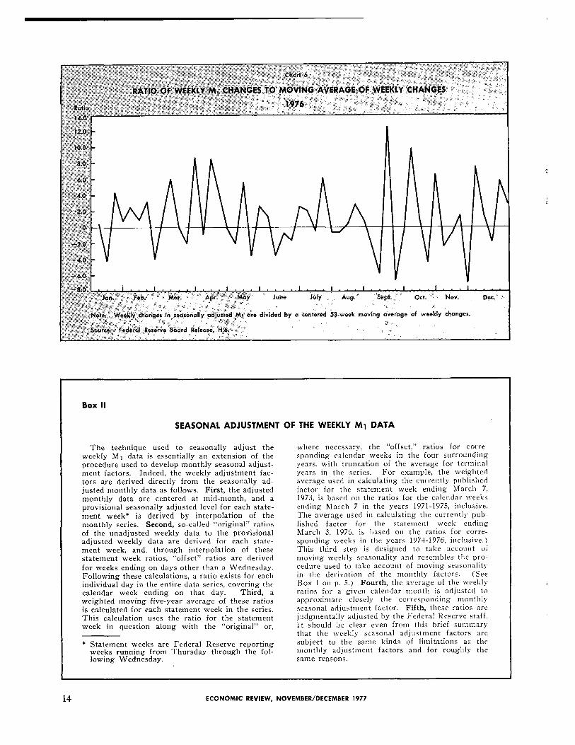
The first point that needs to be made about the
weekly M, data is that they are exceedingly volatile:
the change in Ml this week-whether measured in dollars or as a percentage growth rate-is likely to
be very different from the change next week. Chart 6 provides a visual demonstration of this point using
preiiminary 1976 data. Each point on the graph
shows the ratio of the dollar change in seasonally ad-
justed M, during a given week to a moving 53-week
average of weekly changes centered on that week. As the chart indicates, there are both wide variations in weekly growth over the year as a whole and, in many instances, sharp fluctuations from one week
to the next.
Chart 6 suggests that there is little if any system-
atic relationship between weekly changes in the level
of Ml-viewed either individually or over a period
of several weeks-and longer-run trends in the rate
of M1 growth. Nonetheless, as pointed out in the
introduction to this article, the FOMC’s current
procedures for implementing monetary policy tend to focus the attention of both policymakers and finan- cial market participants on the weekly data. Apart
from these procedures, though, the simple fact that the most recent weekly M1 figure is usually the latest information available regarding monetary develop- ments quite naturally stimulates interest. The re- mainder of this section attempts to provide some
perspective for evaluating the informational content
of the weekly statistics. In general, the same kinds of factors that produce variations in the seasonally adjusted monthly R/I1 data also produce variations in the seasonally adjusted weekly MI data. Abstracting again from fundamental changes in underlying eco-
nomic conditions, these factors are : (1) irregular events and (2) changes in the timing and magnitude of seasonal movements not captured by the seasonal adjustment factors used to adjust the data.
FEDERAL RESERVE BANK OF RICHMOND 13
Jirly * _ Aug.” Oct. -~ Nov. Dec.” 4
Box II
SEASONAL ADJUSTMENT OF THE WEEKLY Ml DATA
The technique used to seasonally adjust the weekly Ml data is essentially an extension of the procedure used to develop monthly seasonal adjust- ment factors. Indeed, the weekly adjustment fac- tors arc derived directly from the seasonally ad- justed monthly data as follows. First, the adjusted monthly data are centered at mid-month, and a provisional seasonally adjusted level for each state- ment week* is derived by interpolation of the monthly series. Second, so-called “original” ratios of the unadjusted weekly data to the provisional adjusted weekly data are derived for each state- ment week, and, through interpolation of these statement week ratios, “offset” ratios are derived
for weeks ending on days other than a Wednesday. Following these calculations, a ratio exists for each individual day in the entire data series, covering the calendar week ending on that day. Third, a weighted moving five-year average of these ratios is calculated for each statement week in the series. This calculation uses the ratio for the statement week in question along with the “original” or,
* Statement weeks are Federal Reserve reporting weeks running from Thursday through the fol- lowing Wednesday.
where necessary, the “offset,” ratios for corre- sponding calendar weeks in the four surrounding years, with truncation of the average for terminal years in tile series. For example, the weighted average used in calculating the currently published factor for the statement week ending March 7, 1973, is based on the ratios for the calendar weeks ending h,Iarch 7 in the years 1971.1975, inclusive. The average used in calculating the currently pub- lished factor for the statement week ending March 3, 1976, is Ijased on the ratios for corre- sponding \veeks in the years 19741976. inclusive.) This third step is designed to take account of moving weekly seasonality and resembles the pro- cedure used to take account of moving seasonalit) in the derivation of the monthly factors. (See Box I on p. 5.) Fourth, the average of the weekly ratios for a given calendar month is adjusted to approximate closely the corresponding monthly seasonal adjustment factor. Fifth, these ratios are judgmentally adjusted by the Federal Reserve staff. It should be clear even from this brief summary that the weekly seasonal adjustment factors are subject to the same kinds of limitations as the monthly adjustment factors and for roughly the same reasons.
J
14 ECONOMIC REVIEW, NOVEMBER/DECEMBER 1977
Irregular Events As we have seen, irregular events can have a sizable effect on monthly M1 growth rates. They can also have a marked impact on the weekly data, particularly if the event is of
relatively short duration. Two illustrations from
recent experience are relevant. In late January 1977,
the eastern and midwestern portions of the United
States experienced the most severe winter weather in
several decades, disrupting production and sales ac-
tivity in these areas. Seasonally adjusted M, fell a
total of $3.0 billion over the two statement weeks
ending January 26, compared to declines of only
$100 million and $700 million in the corresponding periods in 1976 and 1975, respectively. It is likely
that the unusual weather was partly responsible. R4ore recently, there was a precipitous $5.0 billion
increase during the statement week ending July 20, 1977. The magnitude of the rise contrasted sharply with the moderate growth typical of mid-July. While
the full explanation for this increase is unclear, the July 13 power failure in New York City, which dis-
rupted interbank settlements there, may have been a
contributing factor. While it is sometimes possible to anticipate irregular events such as these, they are
more often not anticipated, leading in some instances
to substantial market reactions.
Changes in the Magnitude and Timing of Sea- sonal Gains As in the case of the monthly data,
short-run swings in the adjusted kveekly data are also
caused by changes in the magnitude and timing of seasonal movements not captured by the seasonal
adjustment factors. “Distortions” of the adjusted weekly data of this sort result from inherent defi-
ciencies in the procedures used to derive weekly seasonal adjustment factors similar to those discussed
in Section II of this article with respect to the deri- vation of the monthly adjustment factors. (The pro- cedure for seasonally adjusting the weekly h4, data
is outlined briefly in Box II on 11. 14.) There is
evidence that the distortion of the preliminary ad- justed weekly data clue to these deficiencies is siz-
able. The results of one recent study suggest that the mean absolute revision of the preliminary ad- justed data, espressed il! terms of annualized growth rates, is on the order of 13 percentage points.‘“” Two specific cases are discussed below.
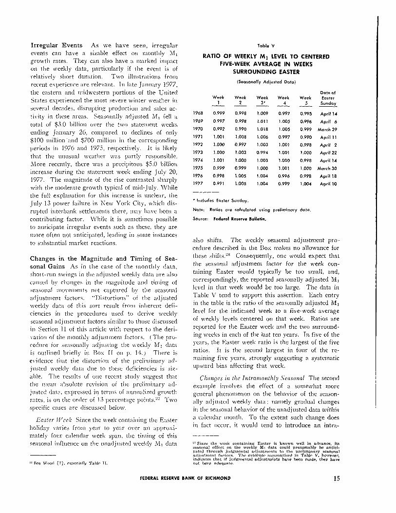
Enstcv Week Since the week containing the Easter
holiday varies from year to year over an al,prosi- mately four calendar week span, the timing of this
seasonal influence on the unadjusted weekly M, data
L” See Wood [7], especially Table II.
Table V
RATIO OF WEEKLY Ml LEVEL TO CENTERED
FIVE-WEEK AVERAGE IN WEEKS
SURROUNDING EASTER
(Seasonally Adjusted Dote)
Date of Week Week Week Week Week Easter
1 2 3* 4 5 Sunday ----__-
1968 0.999 0.998 1.009 0.997 0.995 April 14
1969 0.997 0.998 1.011 1.005 0,996 April 6
1970 0.992 0.990 1.018 1.005 0.999 March 29
1971 1.001 1.008 1.006 0.997 0.990 April 11
1972 1.000 0.997 1.003 1.001 0.998 April 2
1973 1 .ooo 1.003 0.994 1.001 1.000 April 22
1974 1.001 1 .ooo 1.003 1.000 0.998 April 14
1975 0.999 0.999 1.000 1.001 1.000 March 30
1976 0.998 1.005 1.004 0.996 0.998 April 18
1977 0.991 1.005 1.004 0.999 1.004 April 10
* Includes Easter Sunday.
Note: Ratios are calculated using preliminary data.
.SOWC.% Federal Reserve Bulletin.
also shifts. The weekly seasonal adjustment pro- cedure described in the Box makes no allowance for
these shifts.“3 Consequently, one would expect that the seasonal adjustment factor for the week con-
taining Easter would typically be too small, and,
correspondingly, the reported seasonally adjusted M, level in that week would be too large. The data in Table V tend to support this assertion. Each entry in the table is the ratio of the seasonally adjusted M1
level for the indicated week to a five-week average
of weekly levels centered on that week. Ratios are
reported for the Easter week and the two surround- ing weeks in each of the last ten years. In five of the years, the Easter week ratio is the largest of the five
ratios. It is the second largest in four of the re- maining five years, strongly suggesting a systematic
upward bias affecting that week.
Cllangcs in the Intra~uonthly Seasonal The second
example involves the effect of a somewhat more general phenomenon on the behavior of the season- ally adjusted weekly data: namely gradual changes
in the seasonal behavior of the unadjusted data z&l&z
a calendar month. To the extent such change does in fact occur, it would tend to introduce an intra-
“Since the week containing Easter is known well in advance. its seasonal effect on the weekly Ml data could presumably be antici- pated throulrh judgmental adjustments to the preliminary seasonal adjustment factors. The evidence supxnarized in Table V, however. indicates that if judgmental adjustments have been made. they have not been adequate.
FEDERAL RESERVE BANK OF RICHMOND 15

------ ,960 -‘-.--,9&j --- 1968
- 1976
--- 1968
. . . . . . ..-... ,972
- 1976
monthly seasonal movement into the preliminary ad- justed weekly data in a manner analogous to the
impact of the Christmas cycle on the adjusted
monthly data.24
There is ample evidence that intramonthly sea- sonal patterns change. The two panels of Chart 7 depict the intramonthly pattern of the not seasonally adjusted MI data during four separate years span-
ning a 16-year period for the months of July and August. These months were selected since they are less influenced than other months by tax dates and other events that might obscure the evolution. While
this evolution has by no means proceeded at a steady pace, a careful examination of both panels of this
chart suggests that there is now relatively greater
strength in the data during the first half of the month and a sharper decline during the second half. Com-
w Bee Section III, pp. 8-9.
parable data for other months suggest that a similar change may be occurring in these moriths.“5 While
this evolution is not as neat and persistent as the
similar gradual change in the Christmas cycle affect- ing the monthly data, it does appear to be influencing
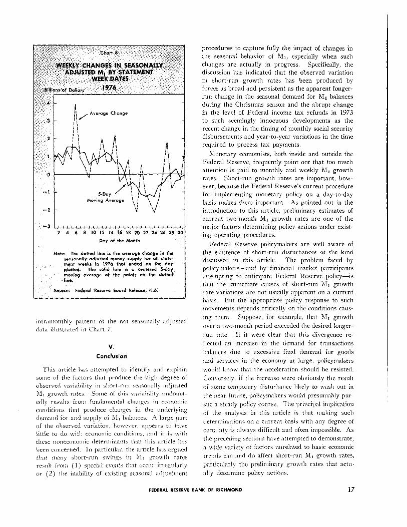
the behavior of the adjusted weekly data. Chart 8 provides evidence supporting this contention. The chart shows the average change in preliminary sea-
sonally adjusted Ml for statement weeks ending on a given calendar day of the month over the 12 months
of 1976, smoothed by a moving average. The chart clearly indicates an upward bias in the seasonall) adjusted movement of Ml in the first half of the
month and a downward bias in the second half of the month, a pattern consistent with the evolution of the
SThe cause of this evolution is not entirely clear. Systematic changes in the intramonthly pattern of Treasury disbursements and receipts, however, are in all likelihood an important eo‘otribut- ing factor.
16 ECONOMIC REVIEW, NOVEMBER/DECEMBER 1977
71 -
Moving Average
-2 -
‘_ -3 IIIIIIIIIIIIIIIILLL 2 4 6 8 10 12 14 16 18 20 22 24 26 28 3
Day of the Month
Note: The dotted line is the average change in the seasonally adjusted money supply for all state-
. ment weeks in 1976 that ended an the day plotted. The solid line is a centered $-day
* moving average of the points on the dotted (. I Jinr, _. : F
So&w: Federal Reserve Board Release, H.6:
intramonthly pattern of the not seasonally adjusted
data illustrated in Chart 7.
V.
Conclusion
This article has attempted to identify and esplnin some of the factors that produce the high degree of observed variability in short-run seasonally adjusted
Ml growth rates. Sonic of this varial)ility undouht-
edly results from fundamental changes in economic conditions that produce changes in the underlying demand for and supply of n1, balances. A large part of the olzerved variation, however, appears to have little ‘ro do with economic conditions, and it is with these noneconomic determinants that this article has lIeen concerned. In particular. the article has argued that many short-run swings in M, growth rates
result frolli ( 1 ) special events that occur irregularly or (2) the inability of existing seasonal adjustment
procedures to capture fully the impact of changes in
the seasonal behavior of Ml, especially when such
changes are actually in progress. Specifically, the discussion has indicated that the observed variation in short-run growth rates has been produced by forces as broad and persistent as the apparent longer-
run change in the seasonal demand for M1 balances during the Christmas season and the abrupt change in the level of Federal income tax refunds in 1973 to such seemingly innocuous developments as the recent change in the timing of monthly social security disbursements and year-to-year variations in the time
required to process tax payments.
Monetary economists, both inside and outside the
Federal Reserve, frequently point out that too much
attention is paid to monthly and weekly M, growth
rates. Short-run growth rates are important, how-
ever, because the Federal Reserve’s current procedure for implementing monetary policy on a day-to-day
basis makes them important. As pointed out in the
introduction to this article, preliminary estimates of
current two-month Ml growth rates are one of the major factors determining policy actions under exist-
ing operating procedures.
Federal Reserve policymakers are well aware of the existence of short-run disturbances of the kind discussed in this article. The problem faced by policymakers-and by financial market participants attempting to anticipate Federal Reserve policy-is that the immediate causes of short-run M1 growth rate variations are not usually apparent on a current
basis. But the appropriate policy response to sucli
movements depends critically on the conditions caus-
ing them. Suppose, for esample, that M1 growth
over a two-month period exceeded the desired longer-
run rate. If it were clear that this divergence re-
flected an increase in the demand for transactions
1)alnnces due to excessive final demand for goods
and services in the economy at large, policymakers
woultl know that the acceleration should be resisted.
Conversely, if the increase were obviously the result
of some temporary disturl~nnce likely to wash out in
the near future, policymakers would presumably pur-
sue ;I steady policy course. The principal implication
of the analysis in this article is that making such
determinations on a current basis with any degree of
certainty is always difficult and often impossible. As
the preceding sections have attempted to demonstrate,
a wide variety of factors unrelated to basic economic
trends can and do affect short-run Ml growth rates,
particularly the preliminary growth rates that actu-
ally determine policy actions.
FEDERAL RESERVE BANK OF RICHMOND 17

Unfortunately, no simple, mechanical solution to
this problem-either for policyrnakers or market ol)-
servers-is likely to be forthcoming. Under these
circumstances, close and eclectic analysis of each
individual fluctuation in short-run growth rates ap-
pears to be the most promising approach. In par-
ticular, the analysis presented in this article suggests
that a detailed familiarity (1 ) with seasonal patterns
in the not seasonally adjusted M1 data at certain
times of the year and (2) with any ongoing or pro-
spective changes in these patterns can assist in evalu-
ating incoming short-run M1 data.
Beyond the question of evaluating incoming data,
however, lies the more fundamental issue of appro-
printe tactical procedures for implementing monetary
policy. Any detailed analysis of this issue is well
lqontl the scope of this article. The preceding de- scription of the difficulties inherent in evaluating
current short-run R/l1 data, however, is bound to raise
doul)ts sl)out the effectiveness of any operating pro-
cedure. such as the esisting one, that focuses largely
on nnnualized short-run growth rates without relating
these short-run growth rates to desired longer-run
growth in n very systenlatic fashion. Suggestions
for improving these procedures have been made else-
where.“G It would appear that tllese suggestions
deserve further attention.
20 See, for example, Poole [Sl.
References
1. Auerbach, Irving M. “Recent Surge in Ml Laid to IRS Delay in Processing Taxes.” The Money Man- ager, May 16, 1977, pp. 4-5.
2. Breimyer, F. and Wenninger, J. “An Estimation of the Effect of Treasury Tax Rebates and Social Security Supplements on M1.” Federal Reserve Bank of New York Research Paper No. 7611, March 1976.
3. Lawler, Thomas. “Seasonal Adjustment of the Money Stock: Problems and Policy Implications.” Economic Review, Federal Reserve Bank of Rich- mond, (November/December 1977)) pp. 19-27.
5. Poole, William. “Interpreting the Fed’s Monetar:y Targets.” Brookings Papers on Economic Aetivitbf, (1st quarter, 1976), pp. 247-259.
6. Poole, William and Lieberman, Charles. “Improving Monetary Control.” Brookings Papevs ox Economic Activity, (2nd quarter, 1972), pp. 293-335.
7. U. S. Department of Commerce. Bureau of the Census. The X-11 Variapzt of the Census Method 1’1 Seasonal Adjustment Progrum, by J. Shiskin, A. II. Young, and J. C. Musgrave. Technical Paper No. 15. Washington, D. C.: 1967.
4. Lombra, Raymond E. and Torto, Raymond G. “The Strategy of Monetary Policy.” Economic Review, Federal Reserve Bank of Richmond, (September/ October 1975), pp. 3-14.
8. Wood, Cynthia W. “Money Stock Revisions.” Eeo- non~ic Commentary, Federal Reserve Bank of Cleve- land, May 16, 1977.
18 ECONOMIC REVIEW, NOVEMBER/DECEMBER 1977
Recommended