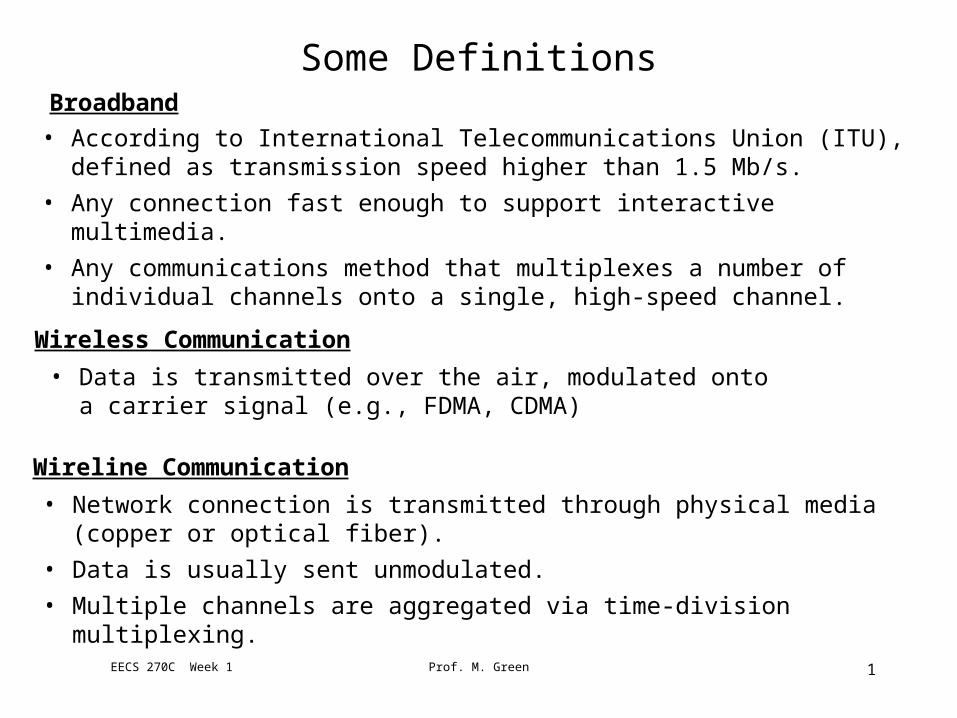
Some Definitions
• According to International Telecommunications Union (ITU), defined as transmission speed higher than 1.5 Mb/s.
• Any connection fast enough to support interactive multimedia.
• Any communications method that multiplexes a number of individual channels onto a single, high-speed channel.
Broadband
Wireline Communication
• Network connection is transmitted through physical media (copper or optical fiber).
• Data is usually sent unmodulated.
• Multiple channels are aggregated via time-division multiplexing.
Wireless Communication
• Data is transmitted over the air, modulated onto a carrier signal (e.g., FDMA, CDMA)
EECS 270C Week 1 1Prof. M. Green
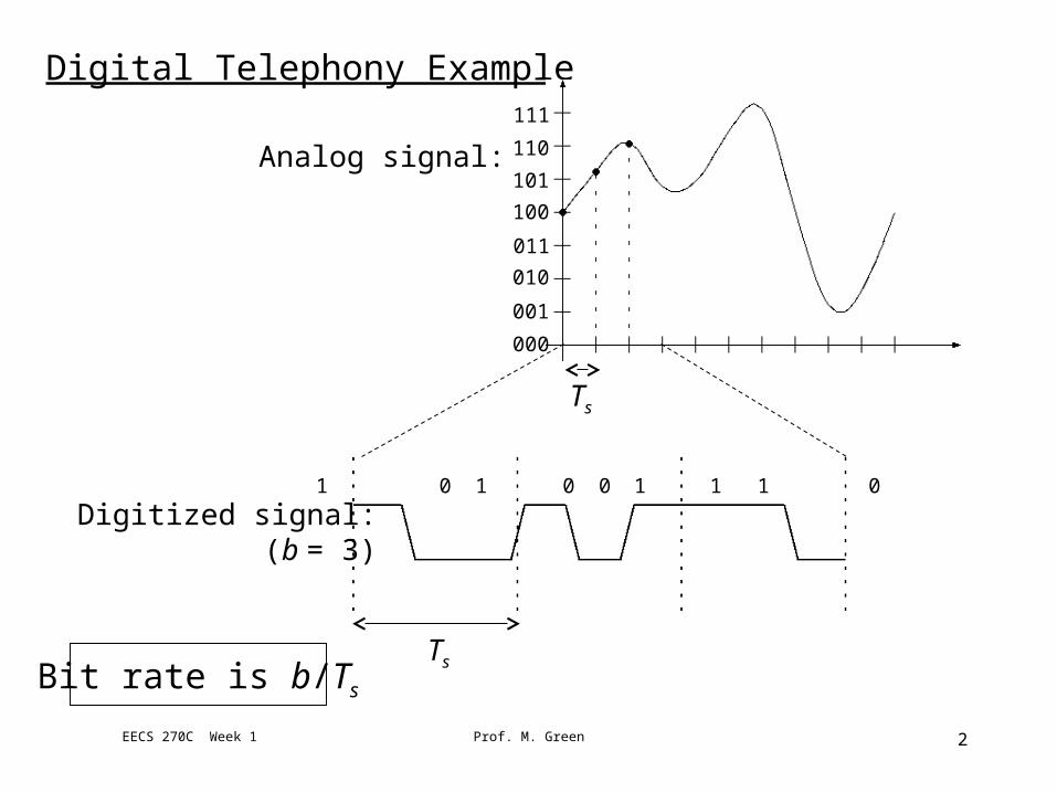
Analog signal:
Bit rate is b/Ts
Digital Telephony Example
000
001
010
011
100
101
110
111
Ts
Ts
Digitized signal:(b = 3)
1 0 0 1 0 1 1 1 0
EECS 270C Week 1 2Prof. M. Green
For digital telephony:
Voice quality requires ~4 kHz bandwidthTs = 125 µs (fs = 8 kHz) b = 8
1 0 0 1 0 1 1 1 0
b bits in Ts
8 kHz X 8 bits (bit rate 64 kb/s) gives “DS0” signal.
User-to-network interface:
24 X DS0
Framing bit
DS1 channel DS1 bits in each TS: 24 X 8 + 1 = 193DS1 bit rate: 193 / 125 µs = 1.544 Mb/s
28 X DS1
188 Framing bits
DS3 channel DS3 bits in each TS: 28 X 193 + 188 = 5592DS3 bit rate: 5592 / 125 µs = 44.736 Mb/s
“T-carrier” system: T1 line carries a DS1 signalT3 line carries a DS3 signal
MUX
MUX
EECS 270C Week 1 3Prof. M. Green

Ethernet
• Invented in 1973 at Xerox PARC
• IEEE 802.3 standard (10 Mb/s) created in 1985
• Used to create Local-Area Networks (LANs)
IEEE ethernet identifiers:
10 BASE 5 -- (10 Mb/s, baseband transmission, 500m max. cable length)
1000 BASE T -- (1 Gb/s, baseband transmission, twisted-pair)
Gigabit/10 Gigabit Ethernet (IEEE Standard 802.3):
1 Gb/s links can be transmitted over twisted-pair copper
10 Gb/s links can be transmitted over copper (short lengths) or fiber.
EECS 270C Week 1 4Prof. M. Green
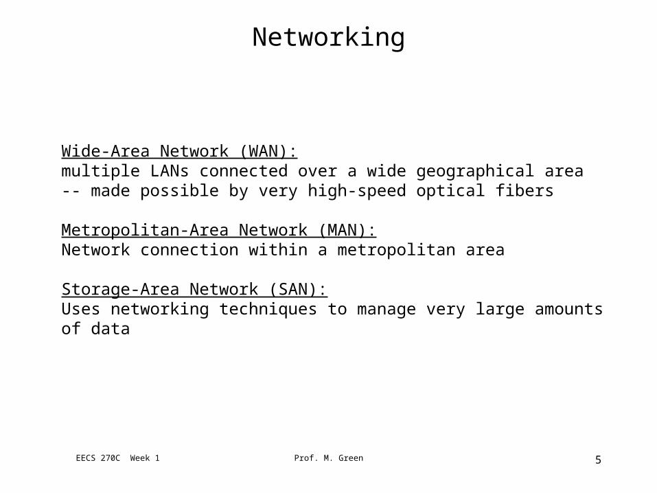
Networking
Wide-Area Network (WAN):multiple LANs connected over a wide geographical area -- made possible by very high-speed optical fibers
Metropolitan-Area Network (MAN):Network connection within a metropolitan area
Storage-Area Network (SAN):Uses networking techniques to manage very large amounts of data
EECS 270C Week 1 5Prof. M. Green
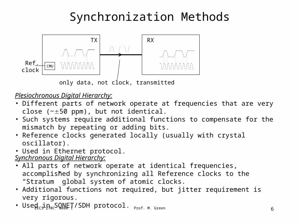
Synchronization Methods
TX RX
CMURef.
clock
only data, not clock, transmitted
Plesiochronous Digital Hierarchy: • Different parts of network operate at frequencies that are very close (~50 ppm), but
not identical. • Such systems require additional functions to compensate for the mismatch by
repeating or adding bits.• Reference clocks generated locally (usually with crystal oscillator).• Used in Ethernet protocol.
Synchronous Digital Hierarchy: • All parts of network operate at identical frequencies, accomplished by synchronizing
all Reference clocks to the “Stratum” global system of atomic clocks.• Additional functions not required, but jitter requirement is very rigorous.• Used in SONET/SDH protocol.
EECS 270C Week 1 6Prof. M. Green
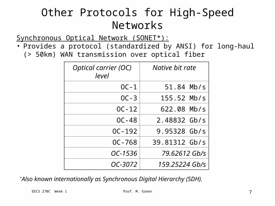
Other Protocols for High-Speed Networks
Synchronous Optical Network (SONET*):• Provides a protocol (standardized by ANSI) for long-haul (> 50km) WAN
transmission over optical fiber
Optical carrier (OC) level
Native bit rate
OC-1 51.84 Mb/s
OC-3 155.52 Mb/s
OC-12 622.08 Mb/s
OC-48 2.48832 Gb/s
OC-192 9.95328 Gb/s
OC-768 39.81312 Gb/s
OC-1536 79.62612 Gb/s
OC-3072 159.25224 Gb/s
*Also known internationally as Synchronous Digital Hierarchy (SDH).
EECS 270C Week 1 7Prof. M. Green
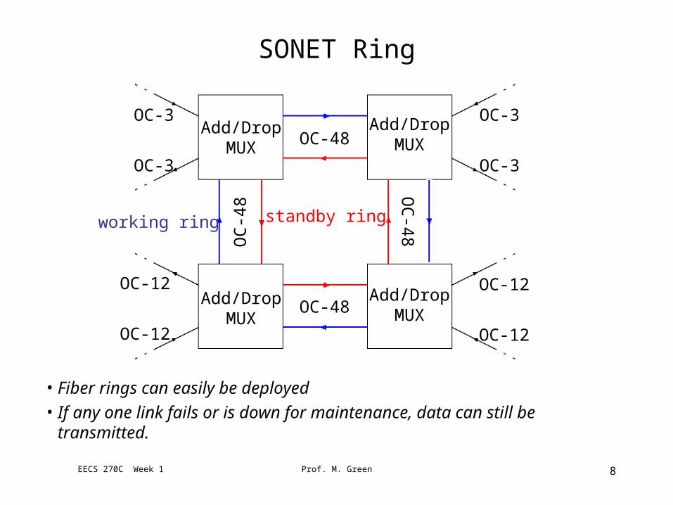
SONET Ring
• Fiber rings can easily be deployed
• If any one link fails or is down for maintenance, data can still be transmitted.
Add/DropMUX
Add/DropMUX
Add/DropMUX
Add/DropMUX
working ring standby ring
OC-48
OC-48
OC
-48
OC
-48
OC-3
OC-3
OC-12
OC-12
OC-3
OC-3
OC-12
OC-12
EECS 270C Week 1 8Prof. M. Green
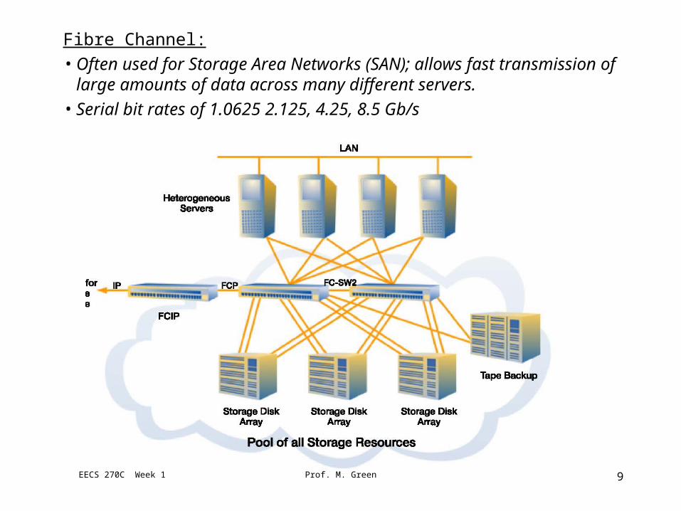
Fibre Channel:
• Often used for Storage Area Networks (SAN); allows fast transmission of large amounts of data across many different servers.
• Serial bit rates of 1.0625 2.125, 4.25, 8.5 Gb/s
EECS 270C Week 1 9Prof. M. Green
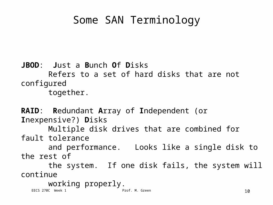
Some SAN Terminology
JBOD: Just a Bunch Of DisksRefers to a set of hard disks that are not configured together.
RAID: Redundant Array of Independent (or Inexpensive?) DisksMultiple disk drives that are combined for fault tolerance and performance. Looks like a single disk to the rest of the system. If one disk fails, the system will continue working properly.
EECS 270C Week 1 10Prof. M. Green
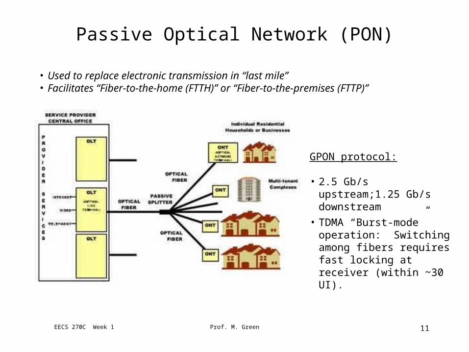
Passive Optical Network (PON)
• Used to replace electronic transmission in “last mile” • Facilitates “Fiber-to-the-home (FTTH)” or “Fiber-to-the-premises (FTTP)”
GPON protocol:
• 2.5 Gb/s upstream;1.25 Gb/s downstream
• TDMA “Burst-mode” operation: Switching among fibers requires fast locking at receiver (within ~30 UI).
EECS 270C Week 1 11Prof. M. Green
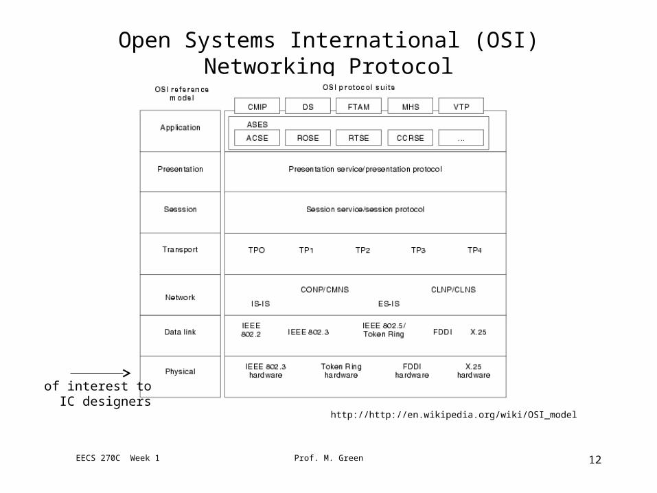
Open Systems International (OSI) Networking Protocol
of interest toIC designers
http://http://en.wikipedia.org/wiki/OSI_model
EECS 270C Week 1 12Prof. M. Green
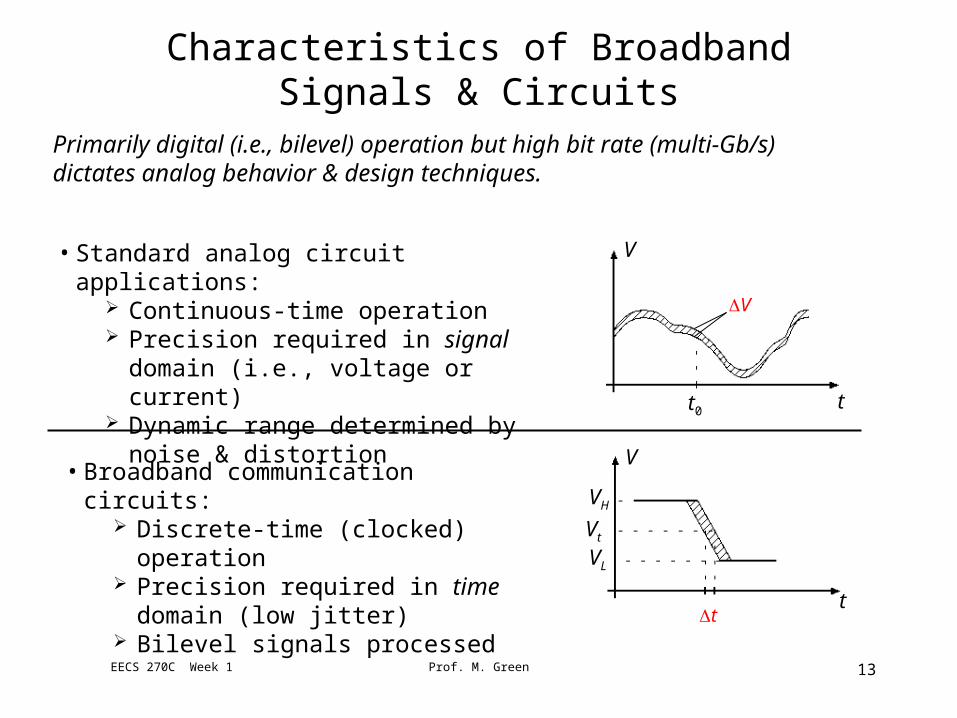
Characteristics of Broadband Signals & Circuits
• Standard analog circuit applications: Continuous-time operation Precision required in signal domain
(i.e., voltage or current) Dynamic range determined by noise
& distortion t
V
t0
V
Primarily digital (i.e., bilevel) operation but high bit rate (multi-Gb/s) dictates analog behavior & design techniques.
t
V
t
VH
Vt
VL
• Broadband communication circuits: Discrete-time (clocked) operation Precision required in time domain
(low jitter) Bilevel signals processed
EECS 270C Week 1 13Prof. M. Green

Non-return-to-zero (NRZ) format (most common):
1 0 1 1 0 1
Return-to-zero (RZ) format:
Tb
“unit interval” (UI)
€
12Tb
• Higher bandwidth RZ signals require faster circuitry than NRZ, but are more easily synchronized due to more transitions.
Binary Data Representations (time domain)
EECS 270C Week 1 14Prof. M. Green

Transition Density is the ratio of transitions to the number of unit intervals in a data stream. A high transition density is desirable in a communication system.
Some Definitions (1)
6 transitions/12 clock cycles transition density = 0.5
Equivalent to density of 0011 repeating pattern
EECS 270C Week 1 15Prof. M. Green
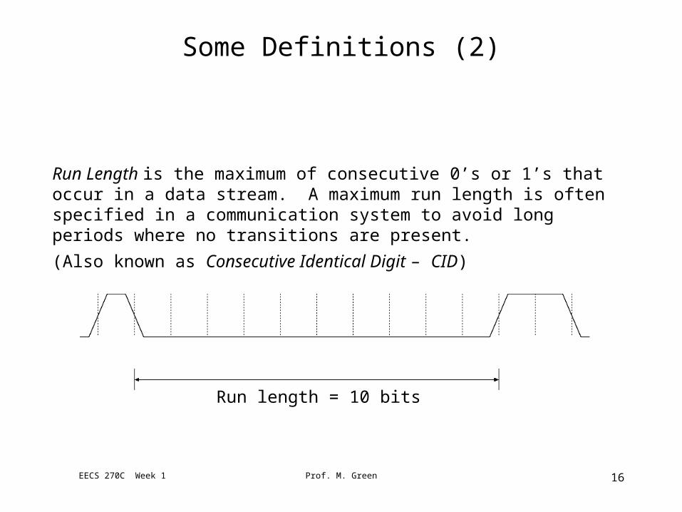
Some Definitions (2)
Run Length is the maximum of consecutive 0’s or 1’s that occur in a data stream. A maximum run length is often specified in a communication system to avoid long periods where no transitions are present.
(Also known as Consecutive Identical Digit – CID)
Run length = 10 bits
EECS 270C Week 1 16Prof. M. Green

Some Definitions (3)
Pseudo-Random Bit Sequence (PRBS) is a repeating pattern that has properties similar to random sequences.
• Parameterized by n, number of DFFs in generator. • Gives almost equal number of 1’s & 0’s• Sequence length = 2n-1; max. run length = n
1001
1100
0010
0101
1110
0111
1011
1001
D1Q3Q2Q1
...
CK
Q1 Q2 Q3D1
€
D1 =Q1 ⊕Q3
23-1 PRBSEECS 270C Week 1 17Prof. M. Green
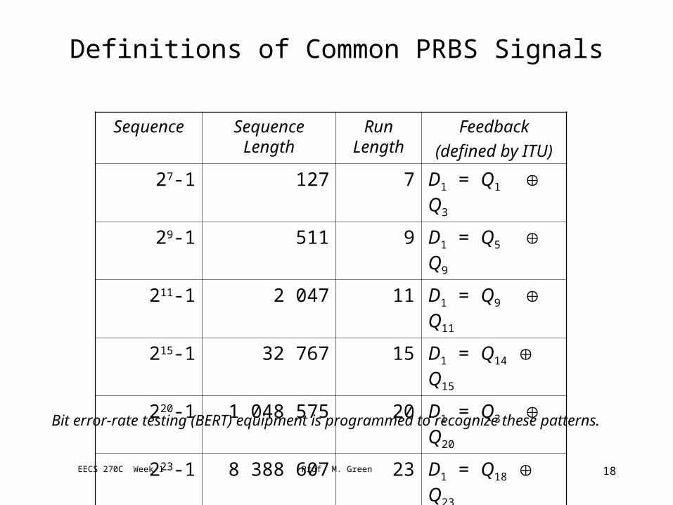
Definitions of Common PRBS Signals
Sequence Sequence Length
Run Length
Feedback
(defined by ITU)
27-1 127 7 D1 = Q1 Q3
29-1 511 9 D1 = Q5 Q9
211-1 2 047 11 D1 = Q9 Q11
215-1 32 767 15 D1 = Q14 Q15
220-1 1 048 575 20 D1 = Q3 Q20
223-1 8 388 607 23 D1 = Q18 Q23
231-1 2 147 483 647 31 D1 = Q28 Q31
Bit error-rate testing (BERT) equipment is programmed to recognize these patterns.
EECS 270C Week 1 18Prof. M. Green

Decimation Properties of PRBS
23-1 PRBS:
PRBS demuxed into 2 parallel channels
Resulting bit sequences are both also 23-1 PRBS!
EECS 270C Week 1 19Prof. M. Green
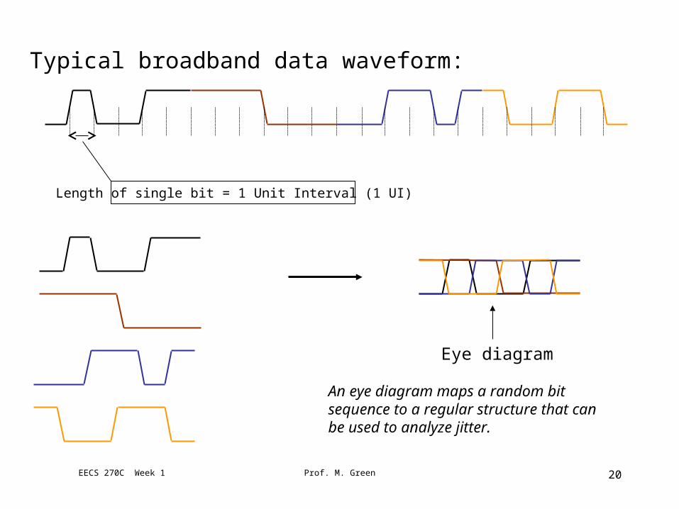
Typical broadband data waveform:
Length of single bit = 1 Unit Interval (1 UI)
Eye diagram
An eye diagram maps a random bit sequence to a regular structure that can be used to analyze jitter.
EECS 270C Week 1 20Prof. M. Green

Close-up of measured eye diagram:
voltage swing
1 UI(Unit Interval)
Zero crossings
trise = tfall
Zero-crossing width indicates jitter.
EECS 270C Week 1 21Prof. M. Green

Types of Jitter (1)Random Jitter (RJ):
• Originates from external and internal random noise sources• Stochastic in nature (probability-based)• Measured in rms units• Observed as Gaussian histogram around zero-crossing• Grows without bound over time
Histogram measurement at zero crossing exhibiting Gaussian probability distribution
EECS 270C Week 1 22Prof. M. Green
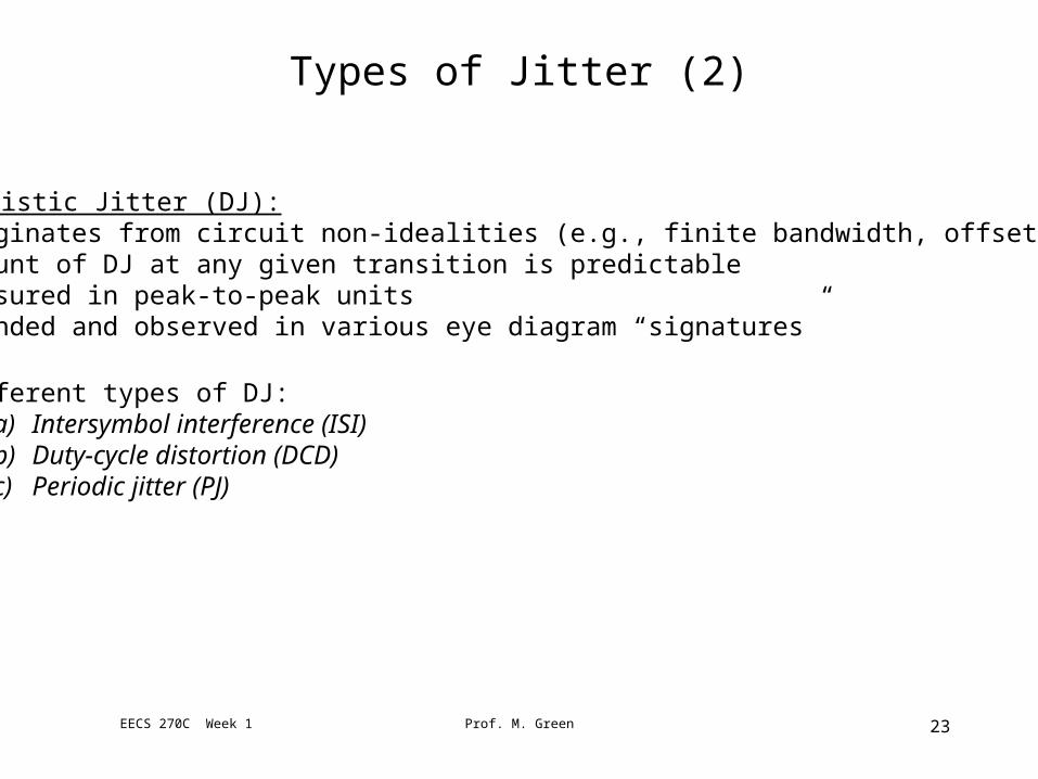
Types of Jitter (2)
Deterministic Jitter (DJ):• Originates from circuit non-idealities (e.g., finite bandwidth, offset, etc.)• Amount of DJ at any given transition is predictable• Measured in peak-to-peak units• Bounded and observed in various eye diagram “signatures”
• Different types of DJ:a) Intersymbol interference (ISI)b) Duty-cycle distortion (DCD)c) Periodic jitter (PJ)
EECS 270C Week 1 23Prof. M. Green
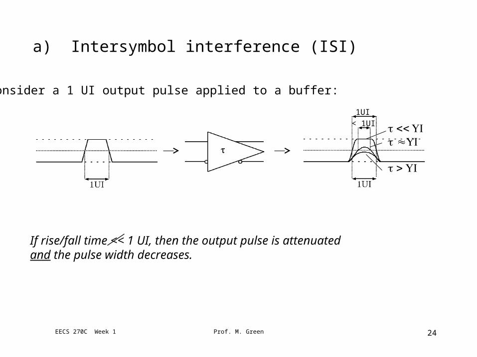
Consider a 1 UI output pulse applied to a buffer:
If rise/fall time << 1 UI, then the output pulse is attenuated and the pulse width decreases.
a) Intersymbol interference (ISI)
€
τ <<UI
€
τ ≈UI
€
τ >UI
1UI
< 1UI
EECS 270C Week 1 24Prof. M. Green

0 0 1
1 0 1
ISI (cont.)
Consider 2 different bit sequences:
t = ISISteady-state not reachedat end of 2nd bit
2 output sequencessuperimposed
ISI is characterized by a double edge in the eye diagram.
EECS 270C Week 1 25Prof. M. Green

Double-edge (DJ) combined with RJ
Effect of ISI on measured eye diagram:
EECS 270C Week 1 26Prof. M. Green

• Occurs when rising and falling edges exhibit different delays• Caused by circuit mismatches
b) Duty cycle distortion (DCD)
Eye diagram with DCD
Crossing offset fromnominal threshold
Nominal data sequence
Data sequence with late falling edges& early rising edges due to threshold shift
t = DCD
Tb 2Tb
EECS 270C Week 1 27Prof. M. Green

c) Periodic Jitter (PJ)
Timing variation caused by periodic sources unrelated to the data pattern.Can be correlated or uncorrelated with data rate.
Clock source withduty cycle ≠50%
Synchronized dataexhibiting correlated PJ
t1 t0
€
PJ =t1 −t0
Uncorrelated jitter (e.g., sub-rate PJ due to supply ripple) affects the eye diagram in a similar way as RJ.
EECS 270C Week 1 28Prof. M. Green

EECS 270C Week 1 Prof. M. Green 29
f
€
1Tb
€
2Tb
€
3Tb
P(f)
Binary Data Representations in Frequency Domain (1)
€
x(t) = bk ⋅p t−kTb( )k
∑A random data signal x(t) can be represented as:
t
€
p(t)
Tb
1
0
where is the bit sequence and p(t) is a unit-interval pulse::
€
bk ∈ −1,+1[ ]
€
Sx f( ) =1Tb
P f( )2=Tb ⋅
sin πfTb( )πfTb
⎡
⎣
⎢ ⎢
⎤
⎦
⎥ ⎥
2
If there is equal probability of low or high logic levels (i.e., dc level is 0), the power spectral density of x(t) is given by:
€
P f( ) =Tb ⋅(sin πfTb )πfTb
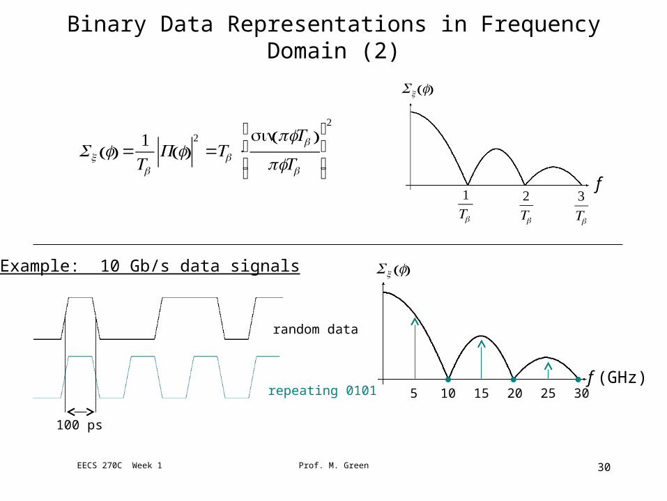
€
Sx f( ) =1Tb
P f( )2=Tb ⋅
sinπfTb( )πfTb
⎡
⎣
⎢ ⎢
⎤
⎦
⎥ ⎥
2
f (GHz)
€
Sx f( )
5 10 15 20 25 30repeating 0101
Example: 10 Gb/s data signals
random data
100 ps
Binary Data Representations in Frequency Domain (2)
f
€
1Tb
€
2Tb
€
3Tb
€
Sx f( )
EECS 270C Week 1 30Prof. M. Green

Transmission over Copper
l
c c
lIdeal transmission line:
For l, c 0, transmission line behaves like a constant delay.
Series loss rs and shunt loss gp cause attenuation and reduce bandwidth.
l
c
rs
gp
l
c
rs
gp
Lossy transmission line:
EECS 270C Week 1 31Prof. M. Green

l
c
rs
gp
l
c
rs
gp
At high frequencies, skin effect causes rs to increase with frequency:
€
H(ω) ≈e−Lα ω
And dielectric loss causes gp to increase with frequency:
€
H(ω) ≈e−Lβω
L = transmission line length; αβ are constants
€
H(ω) =exp−L α ω +βω( ) ⎡ ⎣ ⎢
⎤ ⎦ ⎥For
This results in a very steep drop in a log-log scale …
€
10 logH(ω) =−4.34L⋅α ω +βω( )
EECS 270C Week 1 32Prof. M. Green

f (Hz)
|H(f)| (dB)
108 109 1010 1011
Effect of High-Frequency Loss in Copper Cable
EECS 270C Week 1 33Prof. M. Green

grounded shield
inner conductor (signal)
Purpose of outer conductor:• Shields region inside from external electromagnetic fields• Provides return path
Typical loss @ 100 MHz: 9 dB/foot“ @ 1 GHz: 22 dB/foot
Coaxial cable
EECS 270C Week 1 34Prof. M. Green
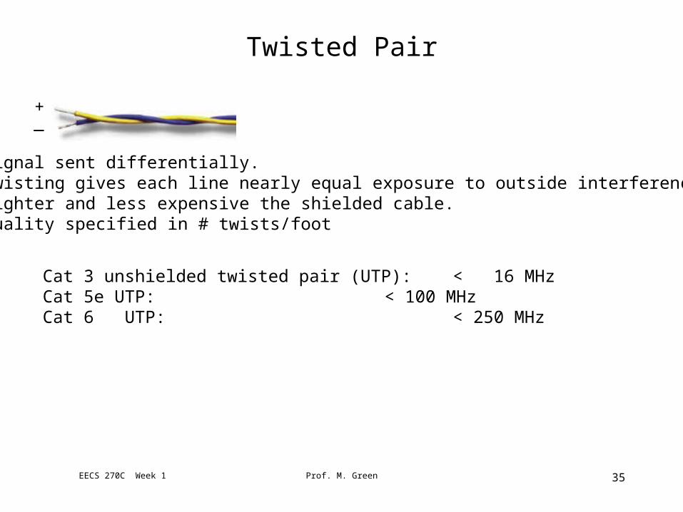
• Signal sent differentially.• Twisting gives each line nearly equal exposure to outside interference.• Lighter and less expensive the shielded cable.• Quality specified in # twists/foot
+_
Cat 3 unshielded twisted pair (UTP): < 16 MHzCat 5e UTP: < 100 MHzCat 6 UTP: < 250 MHz
Twisted Pair
EECS 270C Week 1 35Prof. M. Green
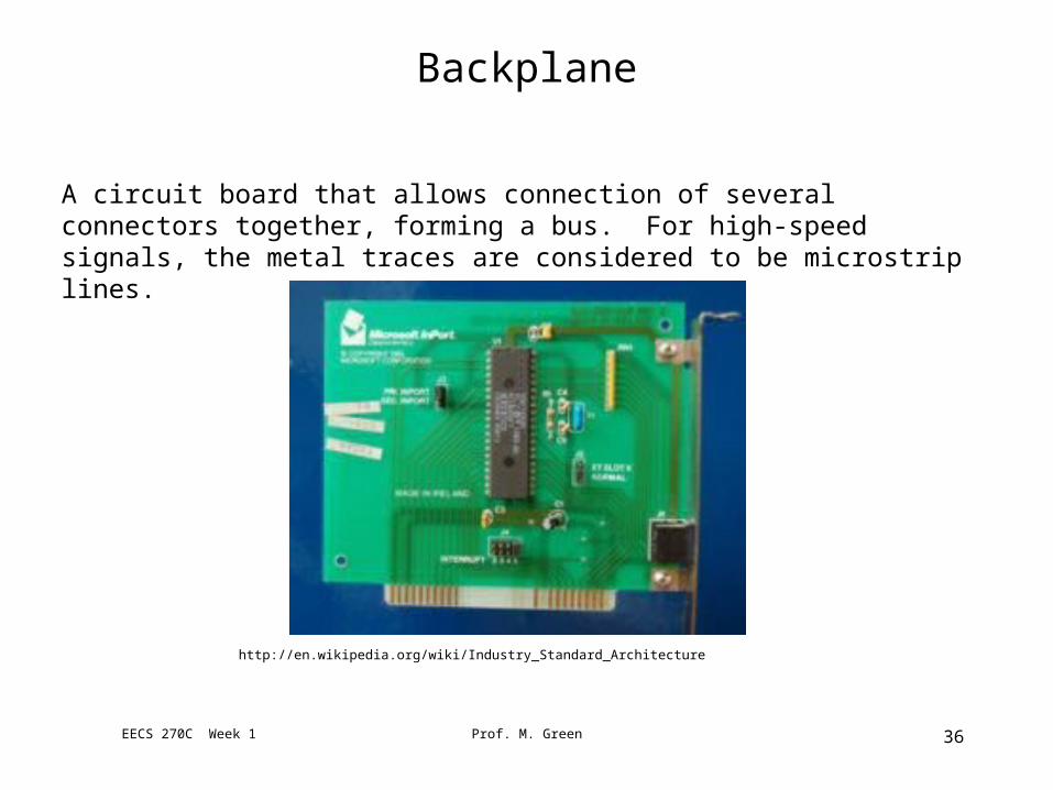
A circuit board that allows connection of several connectors together, forming a bus. For high-speed signals, the metal traces are considered to be microstrip lines.
http://en.wikipedia.org/wiki/Industry_Standard_Architecture
Backplane
EECS 270C Week 1 36Prof. M. Green
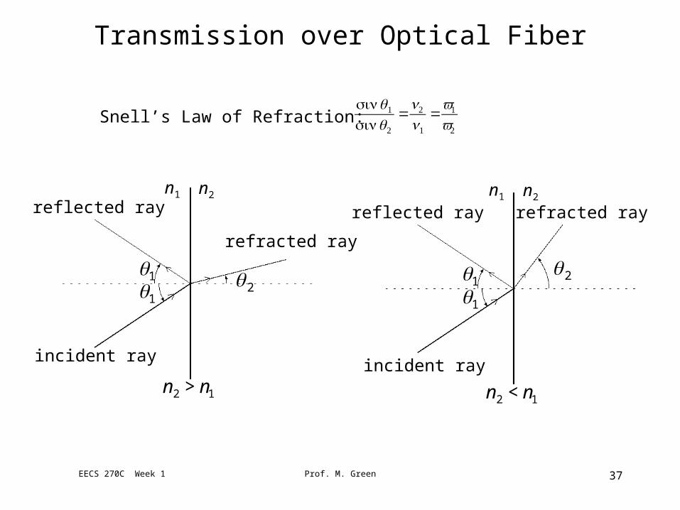
Transmission over Optical Fiber
Snell’s Law of Refraction:
€
sinθ1
sinθ2
=n2
n1
=v1
v2
incident ray
reflected ray
refracted ray
€
θ1
€
θ1
€
θ 2
n1 n2
€
n2 > n1
incident ray
reflected ray refracted ray
€
θ1
€
θ1
€
θ 2
n1 n2
€
n2 < n1
EECS 270C Week 1 37Prof. M. Green

incident ray
reflected ray refracted ray
€
θ1
€
θ1
€
θ 2
n1 n2
€
n2 < n1
Let θ2 = /2:
€
sinθ1 =n2
n1
Then
€
θ c = sin−1 n2
n1
⎛
⎝ ⎜
⎞
⎠ ⎟
For θ1 > θc, light ray is completely reflected.
Total internal reflection
Total Internal Reflection
EECS 270C Week 1 38Prof. M. Green

incident ray
reflected ray refracted ray
€
θ1
€
θ1
€
θ 2
n1 n2
€
n2 < n1
ncore ncladdingncladding
core
cladding
Total internal reflection keeps all optical energy within the core, even if the fiber bends.
€
ncladding<ncore
Optical Fiber Transmission
EECS 270C Week 1 39Prof. M. Green

Advantages of Optical Fibers over Copper Cable
• Very high bandwidth (bandwidth of optical transmission network determined primarily by electronics)
• Low loss
• Interference Immunity (no antenna-like behavior)
• Lower maintenance costs (no corrosion, squirrels don’t like the
taste)• Small & light: 1000 feet of copper weighs approx. 300 lb.
1000 feet of fiber weighs approx. 10 lb.• Different light wavelengths can be multiplexed onto a single
fiber via Dense Wavelength Division Multiplexing (DWM).• 10Gb/s & 40 Gb/s transmission networks are state-of-the art.
EECS 270C Week 1 40Prof. M. Green

850nm(LED) 1310nm 1550nm
Commonly-used wavelengthsFiber Loss vs. Wavelength
EECS 270C Week 1 41Prof. M. Green
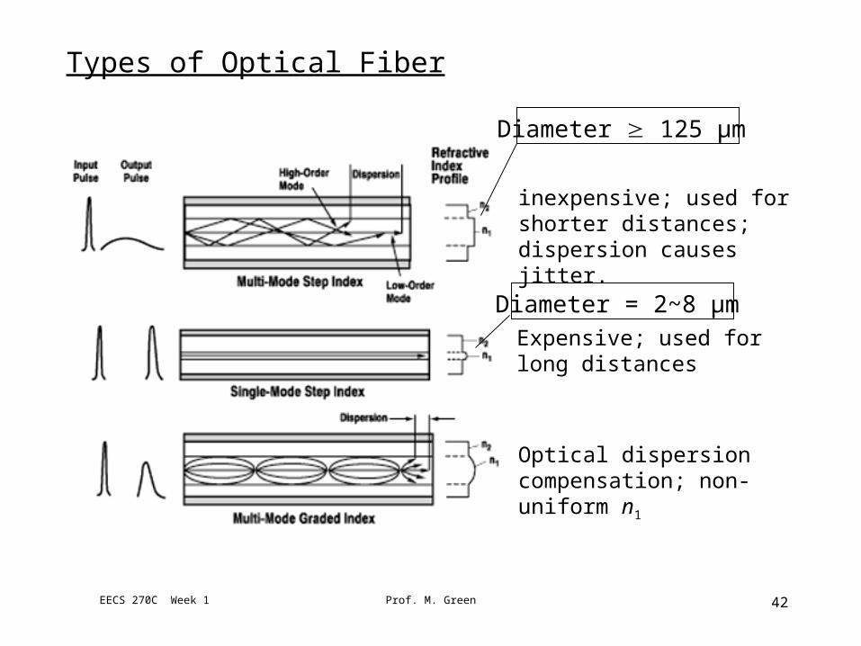
inexpensive; used for shorter distances; dispersion causes jitter.
Diameter 125 µm
Expensive; used for long distances
Diameter = 2~8 µm
Optical dispersion compensation; non-uniform n1
Types of Optical Fiber
EECS 270C Week 1 42Prof. M. Green

Optical Signals
Dr
Modulator
40G
bps
NR
Z s
igna
l
25ps
40 80 f (GHz)-40
λ = 1550nmf = 193 THz
λ = v / f
Laser source
40GHz
193THz f
0.32
1550 λ (nm)
EECS 270C Week 1 43Prof. M. Green
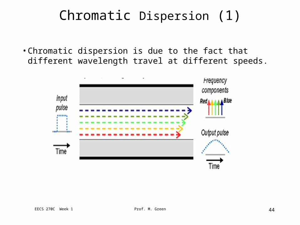
Chromatic Dispersion (1)
• Chromatic dispersion is due to the fact that different wavelength travel at different speeds.
EECS 270C Week 1 44Prof. M. Green
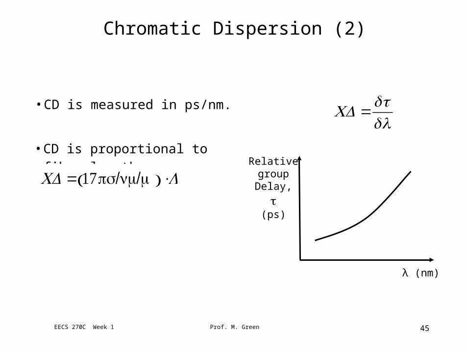
Chromatic Dispersion (2)
RelativegroupDelay,
τ(ps)
λ (nm)
€
CD=dτdλ
• CD is measured in ps/nm.
• CD is proportional to fiber length:
€
CD= 17 / /ps nm m( ) ⋅L
EECS 270C Week 1 45Prof. M. Green
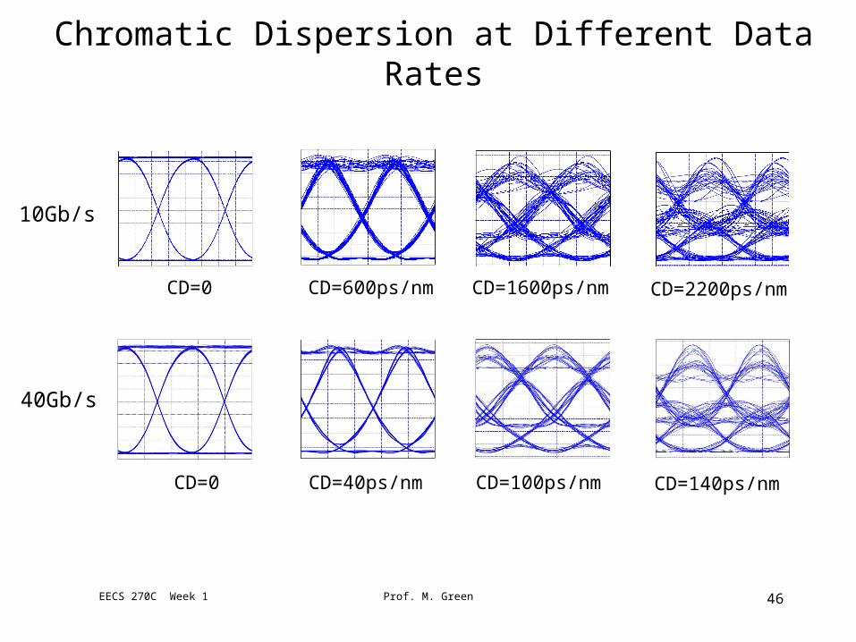
CD=0 CD=600ps/nm CD=1600ps/nm CD=2200ps/nm
10Gb/s
CD=0 CD=40ps/nm CD=100ps/nm CD=140ps/nm
40Gb/s
Chromatic Dispersion at Different Data Rates
EECS 270C Week 1 46Prof. M. Green

Polarization Mode Dispersion
• PMD is due to the fact that light travels at different speed across the two orthogonal polarization states.
• Output contains two delayed images of the input pulse.
EECS 270C Week 1 47Prof. M. Green
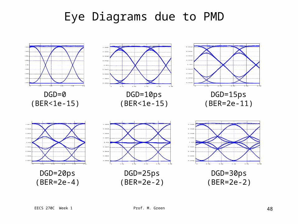
Eye Diagrams due to PMD
DGD=0(BER<1e-15)
DGD=10ps(BER<1e-15)
DGD=15ps(BER=2e-11)
DGD=20ps(BER=2e-4)
DGD=25ps(BER=2e-2)
DGD=30ps(BER=2e-2)
EECS 270C Week 1 48Prof. M. Green
Recommended


![1 195.337 mb 195.338 mb 2kb 195.339 mb 195.34 mb o z o U ... · 195.337 mb 195.338 mb 2kb 195.339 mb 195.34 mb o z o U.] U.] Thiel Hey 1 80.836 80.838 mb 80.84 80.842 mb Figure S7](https://img.dokumen.tips/doc/110x75/5e71a866b2da8320f30922bc/1-195337-mb-195338-mb-2kb-195339-mb-19534-mb-o-z-o-u-195337-mb-195338.jpg)