ORIGINAL ARTICLE
Soil erosion risk assessment of the Keiskamma catchment,South Africa using GIS and remote sensing
Paidamwoyo Mhangara • Vincent Kakembo •
Kyoung Jae Lim
Received: 18 August 2010 / Accepted: 2 July 2011 / Published online: 21 July 2011
� Springer-Verlag 2011
Abstract This paper examines the soil loss spatial pat-
terns in the Keiskamma catchment using the GIS-based
Sediment Assessment Tool for Effective Erosion Control
(SATEEC) to assess the soil erosion risk of the catchment.
SATEEC estimates soil loss and sediment yield within
river catchments using the Revised Universal Soil Loss
Equation (RUSLE) and a spatially distributed sediment
delivery ratio. Vegetation cover in protected areas has a
significant effect in curtailing soil loss. The effect of
rainfall was noted as two pronged, higher rainfall amounts
received in the escarpment promote vegetation growth and
vigour in the Amatole mountain range which in turn pos-
itively provides a protective cover to shield the soil from
soil loss. The negative aspect of high rainfall is that it
increases the rainfall erosivity. The Keiskamma catchment
is predisposed to excessive rates of soil loss due to high soil
erodibility, steep slopes, poor conservation practices and
low vegetation cover. This soil erosion risk assessment
shows that 35% of the catchment is prone to high to
extremely high soil losses higher than 25 ton ha-1 year-1
whilst 65% still experience very low to moderate levels of
soil loss of less than 25 ton ha-1 year-1. Object based
classification highlighted the occurrence of enriched valley
infill which flourishes in sediment laden ephemeral stream
channels. This occurrence increases gully erosion due to
overgrazing within ephemeral stream channels. Measures
to curb further degradation in the catchment should thrive
to strengthen the role of local institutions in controlling
conservation practice.
Keywords Soil erosion � RUSLE � SATEEC GIS �Remote sensing
Introduction
Soil erosion by water is a major environmental problem
that threatens the ecological function of terrestrial and
aquatic systems worldwide (Olderman 1994; Nyakatawa
et al. 2001). It is estimated that 85% of global land
degradation is associated with soil erosion and close to
5 Mg ha-1 year-1 of productive topsoil is lost to lakes and
oceans in Africa (Oldeman et al. 1990; Angima et al.
2003). Flugel et al. (2003) predict that soil erosion will
become more severe in Southern Africa due to population
increases and climatic changes. More than 70% of South
Africa is affected by soil erosion of varying intensities
(Garland et al. 2000; Le Roux et al. 2008). Le Roux et al.
(2008) highlight that the Eastern Cape Province has one of
the highest erosion potentials in South Africa.
Soil erosion is a natural process and relates to the
entrainment and transportation of earth materials across a
given surface. Soil loss is defined as the amount of material
that is actually removed from a particular slope (Renard
et al. 1997); and is one of the major indicators of envi-
ronmental degradation. The negative effects caused by soil
erosion on soil degradation, hydrological systems, agri-
culture, water quality and the environment in general have
long been established and the impacts of soil erosion
continue to pose severe threats to human sustenance (Lal
1998). The impacts of soil erosion include loss of fertile
P. Mhangara (&) � V. Kakembo
Department of Geosciences, Nelson Mandela Metropolitan
University, Port Elizabeth, PO Box 77000, South Africa
e-mail: [email protected];
K. J. Lim
Department of Regional Infrastructure Engineering,
Kangwon National University, Kangwon, Chuncheon, Korea
123
Environ Earth Sci (2012) 65:2087–2102
DOI 10.1007/s12665-011-1190-x

topsoil, decline of soil productivity and reduction in water
quality in river networks. Reservoir sedimentation is one of
the direct impacts of soil erosion that exacerbates water
management problems in Southern Africa (Flugel et al.
2003). The economic and environmental impacts of
accelerated soil erosion are difficult to quantify because of
its extent, magnitude, rate and complexity of the processes
related to it (Lal 1994).
Timely and accurate estimation of soil loss or evaluation
of soil erosion risk is now regarded as an issue of high
priority. Many models have been developed to estimate soil
loss (Wischmeier and Smith 1978; Nearing et al. 1989;
Lim et al. 2005). Among them, the Universal Soil Loss
Equation (USLE) (Wischmeier and Smith 1978), Soil and
Water Assessment Tool (SWAT) (Arnold et al. 1998), Soil
Erosion Model (EUROSEM) (Morgan et al. 1998) and
Water Erosion Prediction Project (WEPP) (Flanagan and
Nearing 1995) have been widely used. The USLE has been
used successfully to estimate soil erosion potential for
nearly 40 years (Dennis and Rorke 1999; Kinnell 2000).
Process-based erosion models have limited use due to
intensive data and computation requirements. The Revised
Universal Soil Loss Equation (RUSLE) was developed on
the basis of substantial modifications of the USLE and its
database to more accurately estimate rainfall erosivity (R),
soil erodibility (K), land cover management (C), conser-
vation practice factor (P) factors, and soil erosion (Renard
et al. 1991). The RUSLE includes the analysis of data that
was not previously included in the USLE, and an update of
the theory describing hydrologic and erosion processes.
Renard et al. (1994) provide a detailed summary of the
differences between USLE and RUSLE. Prominent modi-
fications include corrections of the R factor, new equations
based on the ratio of rill to interrill erosion that accom-
modate complex aspects LS factor and the implementation
of new subfactors for calculating the C factor and the new
P factor (Renard et al. 1991). Notwithstanding these
modifications, the RUSLE model has retained the same
fundamental structure as the USLE (Renard et al. 1994).
The RUSLE model has been used extensively in pre-
dicting soil loss around the world. Wischmeier and Smith
(1978) originally developed the USLE for soil erosion
estimation in croplands on gently sloping topography.
While the RUSLE model has gained acceptance for use at
river catchment and regional scales (Fu et al. 2005; Onori
et al. 2006; Le Roux et al. 2008), USLE and RUSLE were
initially developed to estimate soil erosion at small hill-
slope and plot scale (Wischmeier and Smith 1978). The
SATEEC model can be used for soil erosion risk assess-
ment at watershed scale because of the sediment delivery
ratio (SDR) module integrated in it (Lim et al. 2005; Park
et al. 2010). The SDR is defined as the ratio of sediment
yield to the total surface erosion as affected by catchment
topography, land cover, sediment sources, transport system
and texture of eroded material (Walling 1988; Bhattarai
and Dutta 2007). The concept of SDR encapsulated within
the RUSLE based SATEEC model is an important para-
digm at catchment scale since significant sediment depo-
sition occurs within the catchment before it reaches the
catchment outlet (Bhattarai and Dutta 2007). The SATEEC
model is thus a substantial improvement of the RUSLE
model since it incorporates spatially disturbed sediment
delivery ratios to compute soil loss from rill and interrill
erosion.
Mapping soil erosion in large areas using traditional
methods is a difficult task. The use of remote sensing in
conjunction with GIS techniques makes soil erosion esti-
mation and its spatial distribution attainable at a higher
accuracy and lower cost (Wang et al. 2003). The integrated
application of remote sensing, GIS and RUSLE provides
the potential to estimate soil erosion loss on a cell-by-cell
basis (Millward and Mersey 1999). Soil erosion risk was
assessed successfully using RUSLE by Boggs et al. (2001)
using a Digital Elevation Model (DEM) and land-unit
maps. Related studies also successfully applied the RUSLE
model to soil erosion risk mapping using remote sensing
and GIS techniques (Bartsch et al. 2002; Wang et al. 2003).
The RUSLE parameters can be altered significantly by
human activities. The C factor can be changed by defor-
estation; the P factor can be transformed by shifting
community environmental practices and the L factor by
changing the dimensions of the fields.
Sediment analysis provides an integrated view of sedi-
ment sources, transfers, sinks and outputs of a drainage
basin, and draws together the many aspects of erosion,
sediment mobilization, transport, storage and yield.
According to a review by Le Roux et al. (2007) of erosion
assessment projects conducted in South Africa, the evalu-
ation of soil erosion risk within the context of environ-
mental degradation has not attracted sufficient scientific
attention in the Eastern Cape Province of South Africa. In
particular, soil erosion modelling that integrates sediment
delivery ratios in GIS has not been undertaken. Further-
more, while the use of remote sensing has gained attention
in mapping soil erosion (Marker et al. 2001; Flugel et al.
2003; Taruvinga 2009), the application of object oriented
classification techniques to map soil erosion phenomena
has not yet been explored.
Thus, the objectives of this study are:
1. To determine the spatial patterns of soil loss in the
Keiskamma catchment using a GIS based RUSLE
model that integrates sediment delivery ratios to assess
the environmental health status of the catchment.
2. To map gully erosion surfaces and valley infill in
ephemeral stream channels using object oriented
2088 Environ Earth Sci (2012) 65:2087–2102
123

classification as a means of demonstrating the major
sediment transfer processes operating in the Keiskamma
catchment. Sediments are transferred mostly from rills
and gullies (sediment sources) into ephemeral stream
channels which act as sediment sinks.
Study area
The Keiskamma catchment is located in the Eastern Cape
Province of South Africa, and falls within the greater
Amatola catchment (Fig. 1). It is largely constituted by
nucleated communal settlements designed during the bet-
terment programme of the apartheid era in the 1960s and
1970s. Small towns such as Keiskamma, Alice, Hogsback
and Dimbaza are also found within the catchment. Forest
plantations are found along the Amatola mountain range.
The catchment is characterized by three topographic zones
which are the escarpment zone or mountain highlands, the
coastal plateau and the coastal belt (DWAF 2004). The
coastal belt extends into the catchment for approximately
20 km. The coastal plateau covers most of the catchment
with altitudes ranging from 600 to 900 m above mean sea
level and reaches the base of the Amatola mountain range.
Fig. 1 Map showing the
location of the Keiskamma
catchment in South Africa
Environ Earth Sci (2012) 65:2087–2102 2089
123

The escarpment zone has elevations of up to 1,938 m and
is located between the catchment divide and the coastal
plateau. The incised Keiskamma River valley bisects the
plateau and coastal belt.
The escarpment areas are characterized by dense bush
called the valley thicket in the river valleys and indigenous
forest in the mountain zone. Protected areas in the catch-
ment include Middledrift gamepark, the Hogsback and
Keiskamma Nature Reserve along the Amatola mountain
range and the forest plantation areas. Coastal grasslands,
savannah (thornveld or sourveld) vegetation constitute the
coastal belt and coastal plateau. Black and silver wattle
invasions also characterize some parts of the catchment.
The main Keiskamma river has its headwaters in the
Amatola mountains above Keiskammahoek and winds
eastwards for 263 km to drain the into the Indian Ocean at
the Keiskamma estuary (33�170S; 27�290E) located at
Hamburg midway between East London in the north and
Port Alfred in the south. The Keiskamma catchment is
2,745 km2 big. The Tyume River is the main tributary of
the Keiskamma River.
Today the Keiskamma catchment faces severe threat of
land degradation as result of variety of factors such as
overgrazing by cattle, sheep and goat, deforestation due to
wood harvesting, alien plant invasions in post disturbed
areas. Highly erodible soils derived from shales and mu-
stone are prevalent throughout most parts of the catchment
(D’Huyvetter 1985). Rainfalls amounts experienced in the
catchment range as high as 1,600 mm per annum in the
escarpment region and below 300 mm in the some parts of
the catchment, topography seems to have a profound
influence in rainfall distribution in the catchment (Tanga
1992).
Methods
This study applied the RUSLE model in the GIS-based
Sediment Assessment Tool for Effective Erosion Control
(SATEEC) to estimate soil loss and sediment yield for any
location within the Keiskamma catchment using RUSLE
input data and the spatially distributed sediment delivery
ratio. SATEEC is an ArcView extension developed by Lim
et al. (2005), which is an effective tool to estimate soil loss
and sediment yield.
The RUSLE equation (metric) is defined as:
A ¼ R � K � L � S � C � P ð1Þ
where A annual soil loss (ton ha-1 year-1), R rainfall
erosivity factor (MJ mmha-1 year-1), K = soil erodability
factor (ton h MJ-1 mm-1), L slope length factor, S slope
steepness factor, C cover-management factor, and P sup-
porting practices (Renard et al. 1997).
Parameters used for soil erosion assessment
The derivations of the RUSLE parameters required as
inputs in the SATEEC GIS System to predict the average
annual rate of soil loss are discussed in this section. The
key factors that are explored are: rainfall-runoff erosivity
factor (R), soil erodibility factor (K), slope-length and slope
steepness (LS) factors and cover management factor (C).
All datasets were projected to UTM WGS 84 projection
system and resampled to a grid resolution of 20 m.
Rainfall-runoff erosivity factor (R)
Rainfall is a driver of soil erosion processes and its effect is
accounted for by the rainfall-runoff erosivity factor (R) in
the RUSLE equation. The R-factor accounts for the effect
of raindrop impact and also shows the amount and rate of
runoff associated with precipitation events. The R factor is
computed as total storm energy (E) time the maximum
30-min intensity (I30), or EI, and is expressed as the rainfall
erosion index (Renard et al. 1997). Lack of continuous
pluviograph data relating to rainfall intensity motivated the
application of the equation established by Wischmeier and
Smith (1978) to derive the R factor. Climate data for the
Keiskamma catchment were obtained from the Water
Research Commission (WRC 1995a). Rainfall related data
for the catchment spanned a period of 52 years. Rainfall
data were imported into ArcView since all the weather
stations had co-ordinates. Annual and monthly rainfall data
for the Keiskamma catchment obtained over 52 years were
used to calculate the R-factor in this study. The equation
below developed by Wischmeier and Smith (1978) was
used in the computation.
R ¼X12
i¼1
1:735� 10ð1:5 logp2
ip�0:8188Þ ð2Þ
where pi is the monthly amounts of precipitation and p is
annual precipitation. The annual summation of pi2/p is
called the Fournier equation. In recent years, a number of
interpolation methods have been developed in GIS that
are suitable to model rainfall erosivity. Interpolation
methods available in most GIS software include the
inverse distance weighting (IDW), kriging, spline poly-
nomial trend, and natural neighbour methods. In this
study, the rainfall erosivity values for the different sta-
tions were used to interpolate a rainfall erosivity surface
using the IDW technique available in ArcGIS 9.0. The
IDW interpolation method was selected because rainfall
erosivity sample points are weighted during interpolation
such that the influence of rainfall erosivity is most sig-
nificant at the measured point and decreases as distance
increases away from the point.
2090 Environ Earth Sci (2012) 65:2087–2102
123

Soil erodibility factor (K)
Soil erodibility factor (K) in the RUSLE equation is an
empirical measure which expresses the inherent suscepti-
bility of a soil to water erosion as determined by intrinsic
soil properties. The K factor is rated on a scale from 0 to 1,
with 0 indicating soils with the least susceptibility to ero-
sion and whilst 1 indicates soils which are highly suscep-
tible to soil erosion by water. The factor is defined as the
rate of soil loss per rainfall erosion index unit as measured
on a standard plot.
A digital soil classification coverage captured from a
soil map by the Water Research Commission was supplied
by the Department of Water Affairs and Forestry for
integration into the USLE computation (WRC 1995b).
Highly erodible soils derived from shales and mudstones
are prevalent throughout the catchment. Soil forms present
in the catchment include the Glenrosa, Misaphs, Oakleaf,
Shortland, Hutton, Arcadia and Valrivier (Weaver 1991).
These soil forms falls within the lithic, oxidic, cumulic and
melanic soil groups. Small amounts of stable and well
structured soils derived from dolerite are also found in the
upper part of the catchment (D’Huyvetter 1985). The
topsoil is highly vulnerable to erosion due to the dispersive
character of the soils inherited from the underlying geology
and is further exacerbated by the removal of vegetation.
The Mispahs and Glenrosa soil forms of the lithic soil
group and Hutton soils of the oxidic soil group are, how-
ever, the most widespread soil types and were used to
obtain a general characterization of the soil erodibilities in
this study. These soils are predominately sandy loams and
sandy clay loams.
Fieldwork was conducted to collect soil samples to
determine the particle size distribution where the Mispah,
Hutton and Glenrosa soils are the dominant soil types. A
total of 12 random samples were collected for each area
with the dominant soil type; a soil map was used to
determine the spatial distribution of the soil forms in the
field. The co-ordinates for the soil sampling locations were
collected using a Global Position System (GPS). Soil
erodibility was calculated using Eq. 3 developed by Wis-
chmeier and Smith (1978). The equation effectively
describes soil erodibility as a function of the complex
interaction between sand, silt, and clay fractions in the
soil and other factors such as organic matter, soil structure
and profile permeability class. In general, soils become
less erodible with decrease in silt content, regardless
of corresponding increases in the sand or clay fraction
(Wischmeier and Smith 1978).
K ¼ ½ð2:1� 10�4ð12� OM)M1:14 þ 3:25ðS� 2Þþ 2:5ðP� 3ÞÞ=7:59� 100� ð3Þ
where K = soil erodibility factor (ton h MJ-1 mm-1), OM
is soil organic matter content, M is product of the primary
particle size fractions, M = (%silt ? %very fine sand) 9
(100 - %clay), S is soil structure code, P is permeability
class.
The average soil erodibility for each soil type was
computed and added to the soil classification shapefile
database in ArcView 3.3 software. The shapefile was
subsequently converted to a 20 m grid of soil erodibility.
Areas dominated by Mispah, Hutton and Glenrosa soil
forms were assigned a K value of 0.070, 0.080 and 0.078,
respectively. The soil erodibility ratings are consistent with
results obtained by Weaver (1991) and D’Huyvetter (1985)
in the Keiskamma catchment. These values are also in line
with the soil erosion hazard rating for the soils in the
catchment estimated from the South African Binomial Soil
Classification System. A soil erodibility map was then
developed.
Slope-length (L) and slope steepness (S)
The effect of topography on erosion is expressed by the
L and S factors in the RUSLE model. The L and S factors
can be computed in GIS using a number of empirical for-
mulae (Mc Cool et al. 1987, 1989; Desmet and Govers
1996). A DEM was used to derive the L and S parameters
using a slope length function available in ArcView SA-
TEEC GIS-software. The L factor expresses the ratio of rill
erosion (caused by flow) to interrill erosion (raindrop
impact) to find the loss of soil in relation to the standard
plot length of 72.6 ft. Renard et al. (1997) define slope
length as the horizontal distance traversed from the origin
of overland flow to the point where deposition occurs (a
flattened slope) or runoff concentrates into a defined
channel. The slope steepness factor (S) relates to the effect
of the slope gradient on erosion in comparison to the
standard plot steepness of 9%. The effect of slope steepness
is greater on soil loss compared to slope length.
This study uses a method proposed by Desmet and
Govers (1996) to calculate the L and S factors. Besides
interrill and rill erosion, Desmet and Govers (1997) note
through field observations that the two-dimensional
approach of the RUSLE considers ephemeral gully erosion
as a product of flow convergence. In this procedure, the
RUSLE is adapted to a two-dimensional landscape in
which the upslope length is substituted by the unit con-
tributing area which is defined as the upslope drainage area
per unit of contour length. A 20 m DEM created using
contours was used to derive topographic variables such as
slope length and steepness. The equations developed by
Desmet and Govers (1996) were used to calculate L and
S in this study are shown below.
Environ Earth Sci (2012) 65:2087–2102 2091
123

L factor:
L ¼ k22:13
� �m
m ¼ F
1þ Fð Þ F ¼ sin b=0:0896
3ðsin bÞ0:8 þ 0:56
m ¼ððsinð½slop� � 0:01745Þ=0:0896Þ=ð3� powðsinð½slop� � 0:01745Þ; 0:8Þ þ 0:56ÞÞ ð4Þ
where k is the slope length along the horizontal projection
rather along the sloping surface, m is the slope length
exponent and b is slope angle (%). The L factor with
upslope drainage contributing area (Desmet and Govers
1996) was computed as:
where A(i, j) [m] is unit contributing area at the inlet of grid
cell, D is grid spacing and x is shape correction factor.
The S factor was computed thus:
Sði; jÞ ¼10:8 sin bði; jÞ þ 0:03; tan bði; jÞ\0:09
16:8 sin bði; jÞ � 0:50; tan bði; jÞ� 0:09
(ð6Þ
where b(i, j) is the mean slope angle of all sub-grids in the
steepest direction (Mc Cool et al. 1987, 1989). Hillslope
length k is calculated as the grid area divided by the total
length of streams in the same grid.
Cover and management factor (C)
The cover and management factor can be estimated in
various ways depending on the level of information
available. The main factors which control the cover and
management factor are canopy cover, surface vegetation,
prior land use, mulch cover, surface roughness and soil
moisture (Lorentz and Schulze 1995). This wide range of
factors is difficult and costly to estimate and often vary
considerably during the year. A good estimation of the
cover factor which only accounts for the vegetation cover
can be derived rapidly from satellite imagery. Satellite
imagery acquired during the rain season are more suitable
for this application given that soil erosion is most active
and vegetation cover is at its peak during this season. The
cover factor derived from remote sensing is useful in rural
catchments such as the Keiskamma where vegetation is the
dominant ground cover. The effect of vegetation cover as a
control on soil erosion is well established. Vegetation is
regarded as the second most critical factor after topography
(Benkobi et al. 1994; Biesemans et al. 2000). In the RU-
SLE model, the effect of vegetation cover is incorporated
in cover management, the C factor.
The application of the Normalized-Difference Vegeta-
tion Index (NDVI) derived from remotely sensed images
has been proved to be useful in providing an estimate of the
vegetation cover management factor. The NDVI (Near
Infrared - Red)/(Near Infrared ? Red) is a robust vege-
tation index which has been applied successfully in studies
relating to vegetation dynamics. Landsat 5 Thematic
Mapper satellite data acquired on 12 December 2006 was
used to derive the NDVI by computing the ratio (Band
4 - Band 3)/(Band 4 ? Band 3). The NDVI is highly
correlated with the amount of green biomass, and can
therefore be applied successfully to provide information
relating to the green vegetation variability. Studies by Van
der Knijff (1999, 2000) and van Leeuwen (2003, 2005)
provide a more refined and reasonable estimation of the
C-factor using the NDVI.
The Landsat 5 TM image was accurately orthorectified
and terrain corrected using satellite orbital math modelling
method which applies the Toutin’s Low Resolution Model
available in the PCI Geomatica orthoengine software (PCI
Geomatica 10.3 2009). The Universal Transverse Mercator
(UTM) projection in WGS84 was used in the co-registra-
tion. A 2.5 m geocoded panchromatic SPOT band for the
area was used as the reference image and a 20 m resolution
DEM was used to correct for the topographic distortions.
The cubic convolution resampling method was used for
orthorectification. Rectification errors were less than
0.35 pixels (RMSE). Atmospheric corrections using the
Quick Atmospheric Correction algorithm available in ENVI
were applied to Landsat 5 TM image to improve the spectral
fidelity of the satellite data. Accurate orthorectification of
digital satellite imagery ensured that Landsat 5 TM and
other ancillary datasets overlaid perfectly. The following
equation was used to derive the C-factor in this study.
C ¼ exp �aNDVI
ðb� NDVIÞ
� �ð7Þ
where a and b parameters determine the shape of the NDVI
curve. Reasonable results are produced using values of
a = 2 and b = 1.
Lði; jÞ ¼ ðAði; jÞ þ D2Þmþ1 � Aði; jÞmþ1
xmDmþ2ð22:13Þm
L ¼ ðpowð½Flowacc� þ 1000; ð½m� þ 1ÞÞ � powðð½Flowacc�; ½m� þ 1ÞÞðpowð100; ½m� þ 2Þ � powð22:13; ½m�ÞÞ
ð5Þ
2092 Environ Earth Sci (2012) 65:2087–2102
123

Vegetated areas usual have NDVI values much greater
than 0.1 while values less than 0 rarely contain vegetation
and relate to non-photosynthetic materials such as water
and bare soil. A lower vegetation threshold of 0.05 was set,
below which vegetation was envisaged to be absent. The
ability of NDVI in estimating vegetation cover was con-
firmed in the field through extensive ground truthing.
Conservation practice factor (P)
The conservation practice P factor is an important con-
sideration of the RUSLE model. The support practice
factor is defined as the ratio between soil loss with a spe-
cific support practice and the corresponding loss with
upslope and downslope tillage. Renard and Forster (1983)
explain that support practice essentially affects soil erosion
through altering the flow pattern, gradients, or direction of
surface runoff and by reducing the amount and rate of
runoff. Information regarding conservation was obtained
through field observations in the Keiskamma using a GPS.
Shape files for protected areas which receive high priority
in terms of conservation practice were downloaded from
the South African Biodiversity Institute website (SANBI
2009). These conservancy zones were assigned a P factor
of 0.001, reflecting stringent conservation practice in these
areas. Field assessments in the rest of the Keiskamma
catchment revealed that no significant conservation prac-
tices were in place and a P factor of 1 was assigned to
them. The conservation rating ranges from 0.001 to 1, with
a lower P value indicating that a more effective conser-
vation practice is in place to curtail soil erosion.
Overgrazing, thicket degradation, and general neglect of
the environment in the communal areas are evident in most
parts of the catchment. Bennett and Barrett (2007) studied
the grazing management systems in some communal
areas in the Central Eastern Cape including parts of the
Keiskamma catchment and identified three grazing
management systems. The scholars identified the open
access system, where there is complete lack of grazing
management, the controlled system, where grazing is
governed by the community and lastly private grazing,
whereby the landowner takes responsibility for the grazing
on their private land. Field observations in the catchment
indicated that open access and a loose form of community
controlled system seem to be operational in the Keiskamma
catchment.
Sediment delivery ratios (SDR)
An area based method developed by Vanoni (1975) was
used to estimate the sediment delivery ratios (SDR) in the
SATEEC GIS system. This method uses a generalized
curve derived from experimental work in 300 watersheds.
The watershed area at any point in the catchment is com-
puted from the flow accumulation map, which is derived
from the DEM pre-processing to compute the LS factor
(Lim et al. 2005). The power function used to develop the
generalized SDR curve is shown below.
SDR ¼ 0:4724A�0:125 ð8Þ
where, A watershed area (km2).
Accuracy assessment of soil loss
Model validation was done to ascertain the quality of
results produced by the SATEEC model and test the use-
fulness of the model to predict soil loss. The lack of
measured sediment yield data constrained the comparison
of simulated sediment yield values with field derived val-
ues. An accuracy assessment was thus implemented in this
study to only validate the model results in terms of the
presence or absence of soil erosion. The Kappa Analysis
Tool extension developed by Jenness and Wynnes (2005)
Valley infill
Hillslope erosion
Fig. 2 Photographs showing
hillslope erosion and valley
infill in ephemeral streams
Environ Earth Sci (2012) 65:2087–2102 2093
123

in ArcView 3.3 was used for accuracy assessment. The
application is based on the accuracy assessment theory
presented by Congalton and Green (1999). The Kappa
Analysis method, widely used in remote sensing accuracy
assessments is a powerful method used to measure the
agreement between predicted and observed phenomena
(Jenness and Wynnes 2005).
This study applies Cohen’s Kappa to assess the accuracy
of the SATEEC soil loss results. Extensive fieldwork was
carried in the Keiskamma catchment to randomly identify
eroded and non eroded sites and their locations were cap-
tured using a GPS. The SATEEC soil loss classes were
reclassified into two; low soil loss and high soil loss. The very
low and low soil loss classes were reclassified into low soil
loss and the moderate to extremely high soil classes were
reclassified into the high soil loss classes (after Le Roux et al.
2008). The reclassified soil loss results were then compared
with field validated sample points in ArcView 3.3 software.
Mapping valley infill and erosion features
The valley infill phenomenon is widespread in the degraded
ephemeral streams of the central Keiskamma catchment
where sediment accumulation is manifest (see Fig. 2).
Object oriented classification was used to map valley infill
within ephemeral stream channels and erosion features such
as gullies. Sediment accumulation in ephemeral stream
channels (class 1) can be reliably detected using remote
sensing. Other land cover types that were classified include
roads (class 2), erosional surfaces (class 3), mixed forest
(class 4), sparse and degraded vegetation (class 5). A pan
sharpening algorithm called Principal Component Spectral
Sharpening was used for the fusion of Landsat 5 TM and
SPOT 5 panchromatic band to enhance the spatial resolu-
tion of Landsat 5 TM.
The hybrid fused image possesses both the high spectral
resolution of Landsat 5 TM and a high spatial resolution of
2.5 m inherited from the SPOT 5 panchromatic band.
Object oriented image classification was achieved by first
applying multiresolution segmentation at a scale parameter
of 20 before applying the hierarchical classification in
Definiens Developer software (Definiens 2009). Layer
brightness was used to separate bare areas such as eroded
surfaces and roads. The length/width ratio was then used to
separate roads from erosion features, as the former are more
elongated than the latter. Valley infill and dense vegetation
were classified using the NDVI; vegetation vigour within
ephemeral channel valley infill is higher than on hillslopes
and adjacent areas. The separation of mixed forest from
sparse and degraded vegetation was also done using the
NDVI thresholding of image objects. The brightness
parameter is calculated as follows (Definiens 2009):
�cðvÞ ¼ 1
wB
XK
k¼1
wBK �cKðvÞ ð9Þ
where wBK = brightness weight of image layer k with
wBK ¼
0
1
(
K = number of image layers k for calculation; wB = sum
of brightness weight of all image layers k used for
calculation with
Fig. 3 Grid surface of the
Keiskamma catchment showing
the spatial distribution of the
rainfall erosivity factor
2094 Environ Earth Sci (2012) 65:2087–2102
123

WB ¼XK
k¼1
WBK ð9aÞ
where �cKðvÞ = mean intensity of image layer k of image
object v; �cmink = darkest possible intensity value of image
layer k; �cmaxk = brightest possible intensity value of image
layer k.
Accuracy assessment was done to validate the classifi-
cation using ground reference data collected using a GPS.
Results and interpretation
Soil loss
Results for the RUSLE factors which were computed in
this study are presented in Figs. 3, 4, 5, 6 and 7. The
SATEEC RUSLE approach effectively illustrates the spa-
tial distribution of soil loss throughout the Keiskamma
catchment. The soil loss distributions in the catchment are
Fig. 4 Grid surface of the
Keiskamma catchment showing
the spatial distribution of the
soil erodibility factor
Fig. 5 Grid surface of the
Keiskamma catchment showing
the spatial distribution of slope-
length
Environ Earth Sci (2012) 65:2087–2102 2095
123

illustrated by Fig. 8 and the proportions are summarized in
Fig. 9. The total soil loss in the Keiskamma catchment
is 9.27 9 106 ton year-1 over an area of 257,121 ha. The
mean soil loss in the Keiskamma catchment is
36.063 ton ha-1 year-1. Such high sediment yields are not
surprising considering the highly dispersive nature of the
soils and low vegetation cover in abandoned agricultural
fields. Soil erosion is further accelerated by poor rangeland
management. Overgrazing and thicket clearance is evident
in most communal villages. The protracted history of soil
erosion in the Keiskamma catchment is well documented
(Laker 1978; D’Huyvetter 1985). A study by Le Roux et al.
(2008) indicates that the average predicted soils loss for
South Africa is 12.6 ton ha-1 year-1. Their study further
reveals that the Eastern Cape Province has the highest
annual soil loss contribution of 28% with a soil loss rate of
25 ton ha-1 year-1. The mean soil loss in the Keiskamma
catchment obtained are consistent with the high rates of
soil erosion in the Eastern Cape Province if one considers
that the former Ciskei and Transkei areas are the most
degraded. The greater proportion of the Keiskamma falls
within the former Ciskei area.
Fig. 6 Grid surface of the
Keiskamma catchment showing
the spatial distribution of the
vegetation cover factor
Fig. 7 Grid surface of the
Keiskamma catchment showing
the spatial distribution of the
conservation practice factor
2096 Environ Earth Sci (2012) 65:2087–2102
123
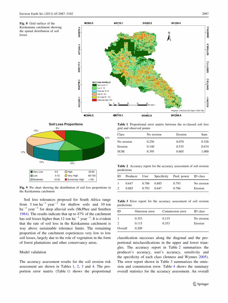
Soil loss tolerances proposed for South Africa range
from 3 ton ha-1 year-1 for shallow soils and 10 ton
ha-1 year-1 for deep alluvial soils (McPhee and Smithen
1984). The results indicate that up to 47% of the catchment
has soil losses higher than 12 ton ha-1 year-1. It is evident
that the rate of soil loss in the Keiskamma catchment is
way above sustainable tolerance limits. The remaining
proportion of the catchment experiences very low to low
soil losses, largely due to the role of vegetation in the form
of forest plantations and other conservancy areas.
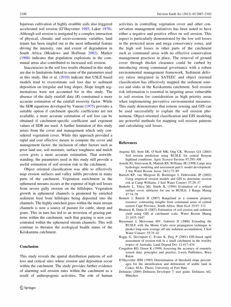
Model validation
The accuracy assessment results for the soil erosion risk
assessment are shown in Tables 1, 2, 3 and 4. The pro-
portion error matrix (Table 1) shows the proportional
classification successes along the diagonal and the pro-
portional misclassifications in the upper and lower trian-
gles. The accuracy report in Table 2 summarizes the
producer’s accuracy, user’s accuracy, sensitivity and
the specificity of each class (Jenness and Wynnes 2005).
The error report shown in Table 3 summarizes the omis-
sion and commission error. Table 4 shows the summary
overall statistics for the accuracy assessment. An overall
Fig. 8 Grid surface of the
Keiskamma catchment showing
the spatial distribution of soil
losses
Soil Loss Proportions
43%
10%12%
17%
13%5%
Very Low 0-5
Low 5-12
Moderate 12-25
High 25-60
Very High 60-150
Extremely High >150
Fig. 9 Pie chart showing the distribution of soil loss proportions in
the Keiskamma catchment
Table 1 Proportional error matrix between the re-classed soil loss
grid and observed points
Class No erosion Erosion Sum
No erosion 0.256 0.070 0.326
Erosion 0.140 0.535 0.674
SUM 0.395 0.605 1.000
Table 2 Accuracy report for the accuracy assessment of soil erosion
predictions
ID Producer User Specificity Pred. power ID class
1 0.647 0.786 0.885 0.793 No erosion
2 0.885 0.793 0.647 0.786 Erosion
Table 3 Error report for the accuracy assessment of soil erosion
predictions
ID Omission error Commission error ID class
1 0.353 0.115 No erosion
2 0.115 0.353 Erosion
Overall 0.209
Environ Earth Sci (2012) 65:2087–2102 2097
123

accuracy of 79.1% was achieved. Khat is the chance-cor-
rected measure of model accuracy, calculated on the actual
agreement between predicted and observed values and the
chance agreement between the row and column totals for
each classification (Jenness and Wynnes 2005). The
Z score of 4.129 and associated P value of 0.0000182
(Table 4) reveal the probability that the SATEEC model
performs better than the random chance at predicting the
occurrence of erosion on the landscape. It can therefore be
concluded that results of the SATEEC model are a good
indication of the soil loss distribution in the Keiskamma
catchment.
Classification of erosion features and valley infill
in ephemeral streams
The ability of the object oriented based multiresolution
segmentation to delineate soil erosion features such as
gullies is illustrated by Fig. 10, where bright white surfaces
can be separated from the other land cover types. The
object oriented classification results are shown in Fig. 11.
Accuracy assessment results (Table 5) for classification of
valley infill and erosional surfaces indicate that object
oriented classification is an effective means of mapping
erosional features and valley infill in ephemeral streams.
An overall accuracy of 92% and kappa coefficient of 0.9
was achieved in the classification. The user’s accuracy for
valley infill and erosional surfaces was 93.8 and 95.3%,
respectively. This classification illustrates the occurrence
of valley infill within ephemeral stream channels and the
presence of gully erosion on the adjacent hillslopes. These
results indicate that both erosion features and sites of
sediment deposition can reliably be mapped using object
oriented classification.
Discussion
The soil loss results show the Keiskamma catchment is
experiencing high proportions of soil loss that are above
provincial and national averages. The results indicate that
the interplay between all the RUSLE factors strongly
influence annual soil loss. It is noticeable that areas asso-
ciated with high rates of soil loss are closely linked to
communal settlements where overgrazing and wood har-
vesting greatly reduce vegetation, leaving the highly
erodible soils vulnerable to the effects of soil erosion. Low
rates of soil loss are associated with the stringent conser-
vation practices in protected areas such as nature reserves,
game parks and forest plantations. Vegetation cover in
mega-conservancy areas has a significant curtailing effect
on soil loss. Despite the buffering effect of vegetation in
the protected zone, high rates of soil loss were noted in its
peripheral areas.
The high soil erosion rates obtained in this study might
be directly linked to the land use history which entailed
land cultivation and abandonment in the 1960s and 1970s.
The betterment programme in the 1960s witnessed exten-
sive cultivation above the sustainable topographic slope
thresholds in a lot of hillslopes in the area (D’Huyvetter
1985). This was subsequently followed by widespread land
Table 4 Summary of overall statistics for the soil erosion accuracy
assessment
Summary of overall statistics
Overall accuracy/sensitivity: 0.791
Overall misclassification: 0.209
Khat: 0.548
Variance: 0.018
Z: 4.129
P: 0.0000182
Gully outlines Gully erosion
Gully segmentation
Fig. 10 Illustration showing the delineation of gullies using multiresolution segmentation on pansharpened satellite imagery
2098 Environ Earth Sci (2012) 65:2087–2102
123

abandonment. The low vegetation cover in abandoned
agricultural fields exacerbates soil erosion in these areas.
The long term effects of cultivation include reduction in
aggregate stability through ploughing and destruction of
the soil organic content. This increases soil erodibility and
renders the soil more vulnerable to soil erosion. These
factors are responsible for the high sediment yields com-
puted in this study. Soil erosion is prevalent throughout
most communal parts of Keiskamma (Hensley and Laker
1975, 1978; D’Huyvetter 1985). Causes of land degrada-
tion in these areas are linked to poor veld management,
overgrazing, uncontrolled burning and deforestation asso-
ciated with harvesting of firewood and medicinal plants.
Fig. 11 Map showing the
object oriented classification of
valley infill and eroded surfaces
in the Keiskamma catchment
Table 5 Accuracy assessment of the object oriented land cover
classification
Class Producer’s
accuracy
User’s
accuracy
Overall
accuracy
Kappa
1 1.000 0.938
2 0.909 0.952
3 0.952 0.91
4 0.700 0.975
5 0.950 0.905
0.921 0.899
1 valley infill, 2 roads, 3 erosional surfaces, 4 mixed forest,
5 degraded forest
Environ Earth Sci (2012) 65:2087–2102 2099
123
Injurious cultivation of highly erodible soils also triggered
accelerated soil erosion (D’Huyvetter 1985; Laker 1978).
Although soil erosion is instigated by a complex interaction
of physical, climatic and socio-economic variables, land
tenure has been singled out as the most influential feature
driving the intensity, rate and extent of degradation in
South Africa (Meadows and Hoffman 2002). Marker
(1988) indicates that population explosions in the com-
munal areas also contributed to increased soil erosion.
Inaccuracies in the soil loss results obtained in this study
are due to limitations linked to some of the parameters used
in this study. Hui et al. (2010) indicate that USLE based
models tend to overestimate soil loss due to sediment
deposition on irregular and long slopes. Slope length seg-
mentations were not accounted for in this study. The
absence of the daily rainfall data (R) constrained a more
accurate estimation of the rainfall erosivity factor. While
the SDR equations developed by Vanoni (1975) provides a
suitable option if catchment specific coefficients are not
available, a more accurate estimation of soil loss can be
obtained if catchment-specific coefficient and exponent
values of SDR are used. A further limitation of this study
arises from the cover and management which only con-
sidered vegetation cover. While this approach provided a
rapid and cost effective means to compute the cover and
management factor, the inclusion of other factors such as
prior land use, soil moisture, surface roughness and mulch
cover gives a more accurate estimation. That notwith-
standing; the parameters used in this study still provide a
useful estimation of soil erosion risk in the catchment.
Object oriented classification was able to effectively
map erosion surfaces and valley infills prevalent in many
parts of the catchment. Vegetation enrichment in the
ephemeral streams occurs at the expense of high soil losses
from severe gully erosion on the hillslopes. Vegetation
growth in ephemeral channels is promoted by enriched
sediment feed from hillslopes being deposited into the
channels. The highly enriched grass within the main stream
channels is now a source of pasture for cattle, sheep and
goats. This in turn has led to an inversion of grazing pat-
terns within the catchment, such that grazing is now con-
centrated within the ephemeral stream channels. This will
continue to threaten the ecological health status of the
Keiskamma catchment.
Conclusion
This study reveals the spatial distribution patterns of soil
loss and critical sites where erosion and deposition occur
within the catchment. The study provides further evidence
of alarming soil erosion rates within the catchment as a
result of anthropogenic activities. The role of human
activities in controlling vegetation cover and other con-
servation management initiatives has been noted to have
either a negative and positive effect on soil erosion. This
aspect is particularly demonstrated by the low soil losses
in the protected areas and mega conservancy zones, and
the high soil losses in other parts of the catchment
such as communal areas with no effective conservation
management practices in place. The removal of ground
cover through thicket clearance could be curbed by
introducing strong communal governance with a robust
environmental management framework. Sediment deliv-
ery ratios integrated in SATEEC and object oriented
classification has effectively mapped the sediment sour-
ces and sinks in the Keiskamma catchment. Soil erosion
risk information is essential in targeting areas vulnerable
to soil erosion for consideration as high priority areas
when implementing preventive environmental measures.
This study demonstrates that remote sensing and GIS can
be used successfully to explain the soil erosion phe-
nomena. Object-oriented classification and GIS modeling
are powerful methods for mapping soil erosion patterns
and calculating soil losses.
References
Angima SD, Stott DE, O’Neill MK, Ong CK, Weesies GA (2003)
Soil erosion prediction using RUSLE for central Kenyan
highland conditions. Agric Ecosyst Environ 97:295–308
Arnold JG, Srinivasan R, Muttiah RS, Williams JR (1998) Large area
hydrologic modeling and assessment part I: model development.
J Am Water Resour Assoc 34(1):73–89
Bartsch KP, van Miegroet H, Boettinger J, Dobrwolski JP (2002)
Using empirical erosion models and GIS to determine erosion
risk at Camp Williams. J Soil Water Conserv 57:29–37
Benkobi L, Trlica MJ, Smith JL (1994) Evaluation of a refined
surface cover subfactor for use in RUSLE. J Range Manag
47:74–78
Bennett J, Barrett H (2007) Rangeland as a common property
resource: contrasting insights from communal areas of central
eastern Cape Province, South Africa. Hum Ecol 35:97–112
Bhattarai R, Dutta D (2007) Estimation of soil erosion and sediment
yield using GIS at catchment scale. Water Resour Manag
21:1635–1647
Biesemans J, Meirvenne MV, Gabriels D (2000) Extending the
RUSLE with the Monte Carlo error propagation technique to
predict long-term average off-site sediment accumulation. J Soil
Water Conserv 55:35–42
Boggs G, Devonport C, Evans K, Puig P (2001) GIS-based rapid
assessment of erosion risk in a small catchment in the wet/dry
tropics of Australia. Land Degrad Dev 12:417–434
Congalton RG, Green K (1999) Assessing the accuracy of remotely
sensed data: principles and practice. Lweis Publishers, Boca
Raton
D’Huyvetter JHH (1985) Determination of threshold slope percent-
ages for the identification and delineation of arable land in
Ciskei. M.Sc. Thesis. University of Fort Hare
Definiens (2009) Definiens Developer 7: user guide. Definiens AG,
Munchen
2100 Environ Earth Sci (2012) 65:2087–2102
123

Dennis MF, Rorke MF (1999) The relationship of soil loss by interill
erosion to slope gradient. Catena 38:211–222
Desmet PJJ, Gover G (1997) Two-dimensional modelling of the
within-field variation in rill and gully geometry and location
related to topography. Catena 29(3–4):283–306
Desmet PJJ, Govers G (1996) A GIS-procedure for automatically
calculating the USLE LS-factor on topographically complex
landscape units. J Soil Water Conserv 51(5):427–433
DWAF (2004) Amatole-Kei area internal strategic perspective WMA
12. Report. 04 August 2004
Flanagan DC, Nearing MA (1995) USDA water erosion prediction
project: hillslope profile and watershed model documentation.
USDA-ARS National Soil Erosion Research Laboratory, West
Lafayette
Flugel WA, Marker M, Moretti S, Rodolfi G (2003) Integrating GIS,
remote sensing, ground truthing and modelling approaches for
regional erosion classification of semiarid catchments in South
Africa and Swaziland. Hydrol Process 17:917–928
Fu BJ, Zhao WW, Chen LD, Zhang QJ, Lu YH, Gulinck H, Poesen J
(2005) Assessment of soil erosion at large watershed scale using
RUSLE and GIS: a case study in the Loess Plateau of China.
Land Degrad Dev 16:7
Garland GG, Hoffman MT, Tod S (2000) Soil degradation. In:
Hoffman MT, Todd S, Ntshona Z and Turner S (eds) A national
review of land degradation in South Africa. South African
National Biodiversity Institute, Pretoria, South Africa, pp 69–107.
http://www.nbi.ac.za/landdeg
Hensley M, Laker MC (1975). Land resources of the Ciskei. In: The
agricultural potential of the Ciskei—a preliminary report.
University of Fort Hare, Alice
Hensley M, Laker MC (1978) Land resources of the consolidated
Ciskei. In: The agricultural potential of the Ciskei. University of
Fort Hare, Alice
Hui L, Xiaoling C, Lim KJ, Xiaobin J, Sagong M (2010) Assessment
of soil erosion and sediment yield in Liao watershed, Jiangxi
Province, China, Using USLE, GIS, and RS. J Earth Sci
21(6):941–953
Jenness J, Wynne JJ (2005) Cohen’s Kappa and classification table
metrics 2.0: an ArcView 3x extension for accuracy assessment of
spatially explicit models: U.S. Geological Survey Open-File
Report OF 2005-1363. USGS
Kinnell PIA (2000) The effect of slope length on sediment
concentrations associated with side-slope erosion. Soil Sci Soc
Am J 64:1004–1008
Laker MC (1978) The agricultural potential of the Ciskei. Amended
report. University of Fort Hare, Alice
Lal R (1994) Soil erosion by wind and water: problems and prospects.
In: Lal R (ed) Soil erosion research methods, 2nd edn. Soil and
Water Conservation Society, St. Lucie Press, pp 1–9
Lal R (1998) Soil erosion impact on agronomic productivity and
environment quality: critical reviews. Plant Sci 17:319–464
Le Roux JJ, Newby TS, Sumner PD (2007) Monitoring soil erosion in
South Africa at a regional scale: review and recommendations.
S Afr J Sci 103(7):7–8
Le Roux JJ, Morgenthal TL, Malherbe J, Pretorius DJ, Sumner PD
(2008) Water erosion prediction at a national scale for South
Africa. Water SA 34:305–314
Lim KJ, Choi J, Kim K, Sagong M, Engel BA (2005) GIS-based
sediment assessment tool. CATENA 64(2005):61–80
Lorentz SA, Schulze RE (1995) Sediment yield. In: Schulze RE
(ed) Hydrology and agrohydrology: a text to accompany the
ACRU 3.00 agrohydrological modelling system (report TT69/
95, pp. AT16-1 to AT16-32). Water Research Commission,
Pretoria
Marker ME (1988) Soil erosion in a catchment near Alice, Ciskei,
Southern Africa. Balkema, Rotterdam
Marker M, Moretti S, Rodolfi G (2001) Assessment of water erosion
processes and dynamics in semiarid regions of southern Africa
(KwaZulu/Natal RSA; Swaziland) using the Erosions Response
Units Concept. Geografia Fisica Dinamica Quaternaria 24:71–83
Mc Cool DK, Brown LC, Foster GR, Mutchler CK, Meyer LD (1987)
Revised slope steepness factor for the Universal Soil Loss
Equation. Trans ASAE 30:1387–1396
Mc Cool DK, Foster GR, Mutchler CK, Meyer LD (1989) Revised
slope length factor for the Universal Soil Loss Equation. Trans
ASAE 32:1571–1576
McPhee PJ, Smithen AA (1984) Applications of USLE in the Republic
of South Africa. Agricultural Engineering in South Africa
Meadows ME, Hoffman MT (2002) The nature, extent and causes of
land degradation in South Africa: legacy of the past, lessons for
the South Africa. University of Cape Town Press, Cape Town
Millward A, Mersey J (1999) Adapting the RUSLE to model soil
erosion potential in a mountainous tropical watershed. Catena
38:109–129
Morgan RPC, Quinton JN, Smith RE, Govers G, Poesen JWA,
Auerswald K, Chisci G, Torri D, Styczen ME (1998) The
European Soil Erosion Model (EUROSEM): a dynamic
approach for predicting sediment transport from fields and small
catchments. Earth Surf Process Landf 23:527–544
Nearing MA, Foster GR, Lane LJ, Finkner SC (1989) A process-
based soil erosion model for USDA-Water Erosion Prediction
Project Technology. Trans ASAE 32:1587–1593
Nyakatawa EZ, Reddy KC, Lemunyon JL (2001) Predicting soil
erosion in conservation tillage cotton production systems using
the revised universal soil loss equation (RUSLE). Soil Tillage
Res 57:213–224
Oldeman LR, Hakkeling RTA, Sombroek WG (1990) World map of
the status of human-induced soil degradation: an explanatory
note. Revised edn. Wageningen/Nairobi: international soil refer-
ence and information. United Nations Environment Programme
Olderman LR (1994) The global extent of soil degradation. In:
Greenland DJ, Saboles T (eds) Soil resilience and sustainable
landuse. Commonwealth Agricultural Bureau International,
Wallingford
Onori F, De Bonis P, Grauso S (2006) Soil erosion prediction at the
basin scale using the revised universal soil loss equation
(RUSLE) in a catchment of Sicily (southern Italy). Environ
Geol 50:1129–1140
Park YS, Kim J, Kim NW, Kim SJ, Jeon J, Engel BA, Jang W, Lim K
(2010) Development of new R, C and SDR modules for the
SATEEC GIS system. Comput Geosci 36(2010):726–734
PCI Geomatica 10.3 (2009) PCI Geomatica Orthoengine manual. PCI
Geomatics Inc
Renard KG, Foster GR (ed) (1983) Soil conservation-principles of
erosion by water, Soil Science Society of America. American
Society of Agronomy, Madison
Renard KG, Foster GR, Weesies GA, Porter JP (1991) RUSLE:
revised Universal Soil Loss Equation. J Soil Water Conserv
46(1):30–33
Renard KG, Foster GR, Yoder DC, McCool DK (1994) RUSLE
revisited: status, questions, answers, and the future. J Soil Water
Conserv 49(3):213–220
Renard KG, Foster FG, Weesies GA, McCool DK, Yoder DC (1997)
Predicting soil erosion by water: a guide to conservation planning
with the revised Universal Soil Loss Equation (RUSLE) (Vol.
Handbook #703). US Department of Agriculture, Washington
SANBI (2009) STEP: conservation priority status. Mega-conservancy
networks. http://bgis.sanbi.org/STEP/priorityStatus.Asp. Acces-
sed 10 June 2009
Tanga LV (1992) Rainfall disparties in the Eastern Cape region: the
case of Alice and Hogsback (1967 to 1987). Unpublished M.Sc.
thesis. University of Fort Hare, Alice, South Africa
Environ Earth Sci (2012) 65:2087–2102 2101
123

Taruvinga K (2009) Gully mapping using remote sensing: case study
in Kwazulu-Natal, South Africa. Masters Thesis. University of
Waterloo
Van der Knijff JM, Jones RJA, Montanarella L (1999) Soil erosion
risk assessment in Italy. Joint Research Center of the European
Commission, NY
Van der Knijff JM, Jones RJA, Montanarella AL (2000) Soil erosion
risk assessment in Europe. Joint Research Center of the
European Commission, NY
van Leeuwen WJD, Sammons G (2003) Seasonal land degradation
risk assessment for Arizona. In: Proceedings of the 30th
international symposium on remote sensing of environment,
2003 November 10–14, Honolulu, HI. ISRSE, Tucson
van Leeuwen WJD, Sammons G (2005) Vegetation dynamics and
erosion modeling using remotely sensed data (MODIS) and GIS.
In: Tenth biennial USDA forest service remote sensing appli-
cations conference, 2004 April 5–9, Salt Lake City, UT. U.S.
Department of Agriculture Forest Service Remote Sensing
Applications Center, Salt Lake City
Vanoni VA (1975) Sedimentation engineering, manual and report
no.54. American Society of Civil Engineers, New York
Walling DE (1988) Erosion and sediment yield research—some
recent perspectives. J Hydrol 100:113–141
Wang GGG, Fang S, Anderson AB (2003) Mapping multiple
variables for predicting soil loss by geostatistical methods with
TM images and a slope map. Photogramm Eng Remote Sens
69:889–898
Weaver AvB (1991) The distribution of soil erosion as a function of
slope aspect and parent material in Ciskei, Southern Africa.
GeoJournal 23(1):29–34
Wischmeier WH, Smith DD (1978) Predicting rainfall erosion
losses—a guide to conservation. Agricultural Handbook 537.
US Department of Agriculture, Washington
WRC (1995a) Precipitation data for South Africa from the WR90
project. WR90: Surface water resources of South Africa 1990
WRC (1995b) Geomorphology: soil groups based on 1989 revised
broad homogeneous natural regions map-Natal University. WR
90: surface water resources of South Africa 1990
2102 Environ Earth Sci (2012) 65:2087–2102
123
Recommended