
Signals and Systems
Continuous-Time Fourier
Transform
Chang-Su Kim
continuous time discrete time
periodic (series) CTFS DTFS
aperiodic (transform) CTFT DTFT

Lowpass Filtering – Blurring or Smoothing
Original Strong LPF
e.g. 21x21 moving
average filter
Less strong LPF
e.g. 11x11 moving
average filter
average

Highpass Filtering – Edge Extraction

CTFT Formula and Its Derivation

Bridge Between Fourier Series and Transform
Consider the periodic signal x(t)
Its Fourier coefficients are
0
0
)sin(
,2
10
1
k
k
k
Tk
T
T
ak
x(t)
t
-T1 0 T1 T-T

Sketch ak on the k-axis
The sketch is obtained by sampling the sinc function.
For each value of k, the signal x(t) has a periodic component with weight ak. So, the above sketch shows the frequency content of the signal x(t).
Bridge Between Fourier Series and Transform
ak
k-2 -1 0 1 2
2T1/T

The same sketch ak on the -axis:
On the -axis, the distance between two consecutive
ak’s is 0=2/T, which is the fundamental frequency.
ak
-20 -0 0 0 20
2T1/T
Bridge Between Fourier Series and Transform
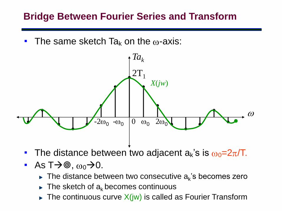
The same sketch Tak on the -axis:
The distance between two adjacent ak’s is 0=2/T.
As T, 00. The distance between two consecutive ak’s becomes zero
The sketch of ak becomes continuous
The continuous curve X(jw) is called as Fourier Transform
Tak
-20 -0 0 0 20
2T1
Bridge Between Fourier Series and Transform
X(jw)
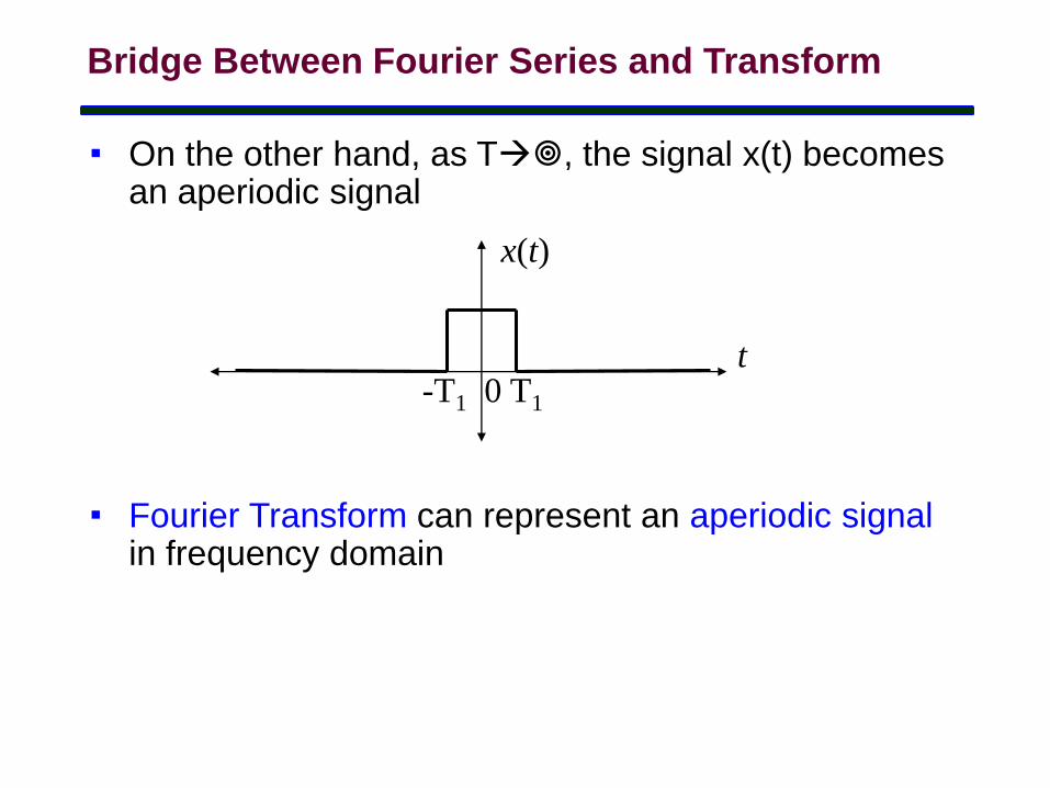
On the other hand, as T, the signal x(t) becomes an aperiodic signal
Fourier Transform can represent an aperiodic signalin frequency domain
x(t)
t-T1 0 T1
Bridge Between Fourier Series and Transform

How can we use this formula for a non-
periodic (aperiodic) function x(t)?
. . .
0 T 2T
)(~ tx
0
x(t)
( ) lim ( )T
x t x t
From CTFS to CTFT: Formal Derivation
( ) lim ( )T
x t x t
0
0
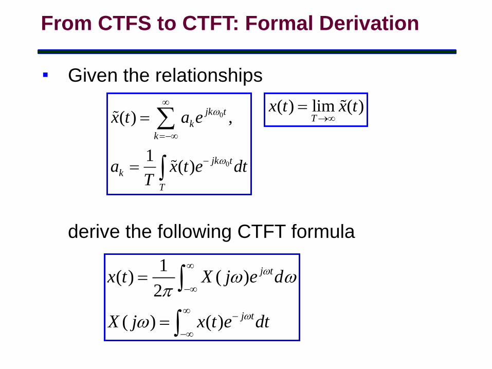
( ) ,
1( )
jk t
k
k
jk t
k
T
x t a e
a x t e dtT
1( ) ( )
2
( ) ( )
j t
j t
x t X j e d
X j x t e dt
Given the relationships
derive the following CTFT formula
From CTFS to CTFT: Formal Derivation

CTFT Formula – Fourier Transform Pair
( ) ( ) j tX j x t e dt
1( ) ( )
2
j tx t X j e d
Forward Transform
Inverse Transform
X(jw) represents the strength of frequency
component at w in x(t)
Time Domain vs. Frequency Domain
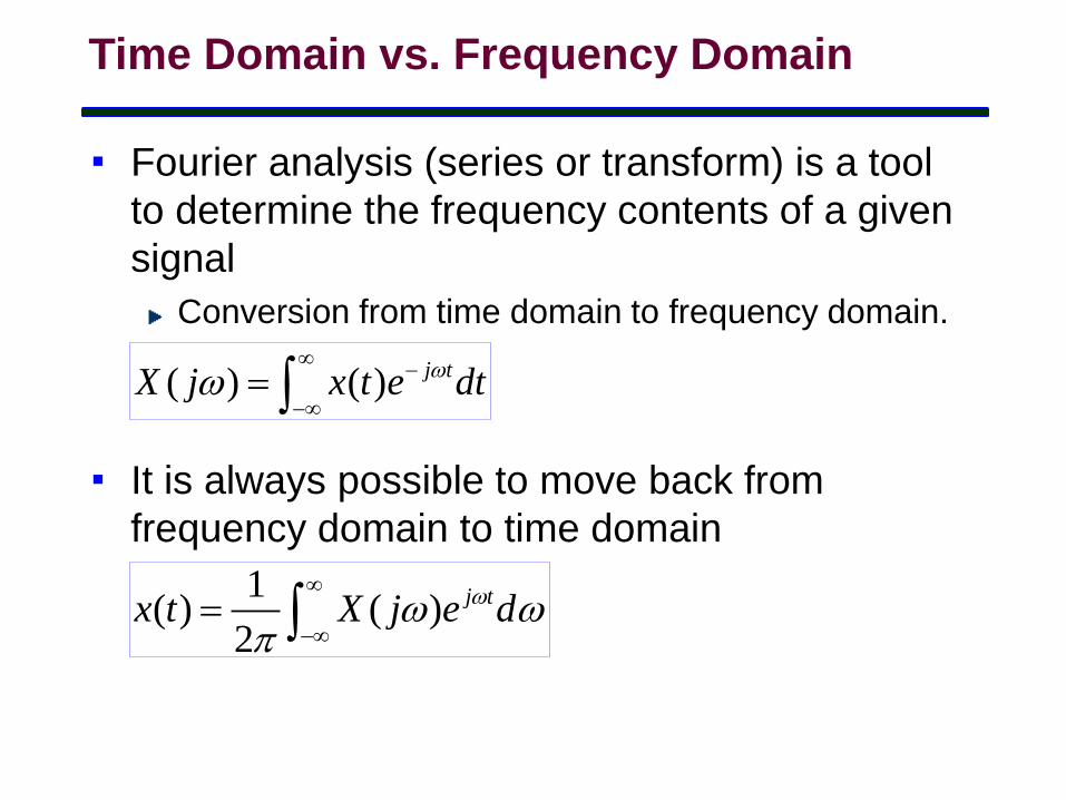
Fourier analysis (series or transform) is a tool
to determine the frequency contents of a given
signal
Conversion from time domain to frequency domain.
It is always possible to move back from
frequency domain to time domain
( ) ( ) j tX j x t e dt
1( ) ( )
2
j tx t X j e d

Some Examples
1)()( )()( F
dtetjXttx tj
t
1
0
Ex 1) Impulse function → constant function

Ex 2) Rectangular pulse → sinc function
1
1
1 11
2sin( ) 2 sinc( )
sin( )where sinc( )
Tj t
T
T Tj e dt T
tt
t
-T1 T1
1
2T1
1T
1T
t
Some Examples
Note the inverse relationship between time and frequency domains

More Examples

Unified Framework for CTFS and CTFT:
Periodic Signals Can Also Be Represented as Fourier Transform

Fourier Transform for Periodic Signals
Consider the inverse Fourier transform of
So, we can deduce that
k
k kaj )(2)( 0
0 Fourier
0( ) ( ) 2 ( )jk t
k k
k k
x t a e j a k
. . .
0 02 03
32 a
. . .

ja
jattx SF
2
1 ,
2
1)sin()( 11
..
0
Fourier Transform for Periodic Signals
Ex 1) sin function
0
0
)( j
/j
-/j
2
1)cos()( 11
..
0 aattx SF
0 0
)( j
Ex 2) cos function

0/ 2
. .
/ 2
1 1( ) ( ) ( )
2 2( ) ( )
Tjk tF S
kT
k
x t t kT a t e dtT T
kX j
T T
Fourier Transform for Periodic Signals
Ex 3) Fourier transform of impulse trains
1
T 2T
…
2/T
2/T 4/Tt
... …… F
)( jX)(tx

Properties of CTFT

Properties of CTFT
1. Linearity
2. Time shifting
3. Conjugation and conjugate symmetry
4. Differentiation and integration
( ) ( ) ( ) ( )Fa x t b y t aX j bY j
0
0( ) ( )j tFx t t e X j
* *
*
( ) ( )
( ) ( ) [ ( ) real]
Fx t X j
X j X j x t
( )( )
1( ) ( ) (0) ( )
F
tF
dx tj j
dt
x d X j Xj

Properties of CTFT
5. Time and frequency scaling
6. Parseval’s relation
7. Duality
)()(
)(||
1)(
jtx
a
j
aatx
F
F
djdttx 22 |)(|
2
1|)(|
)(2)( )()( FF gjtGjGtg
Convolution Property of CTFT
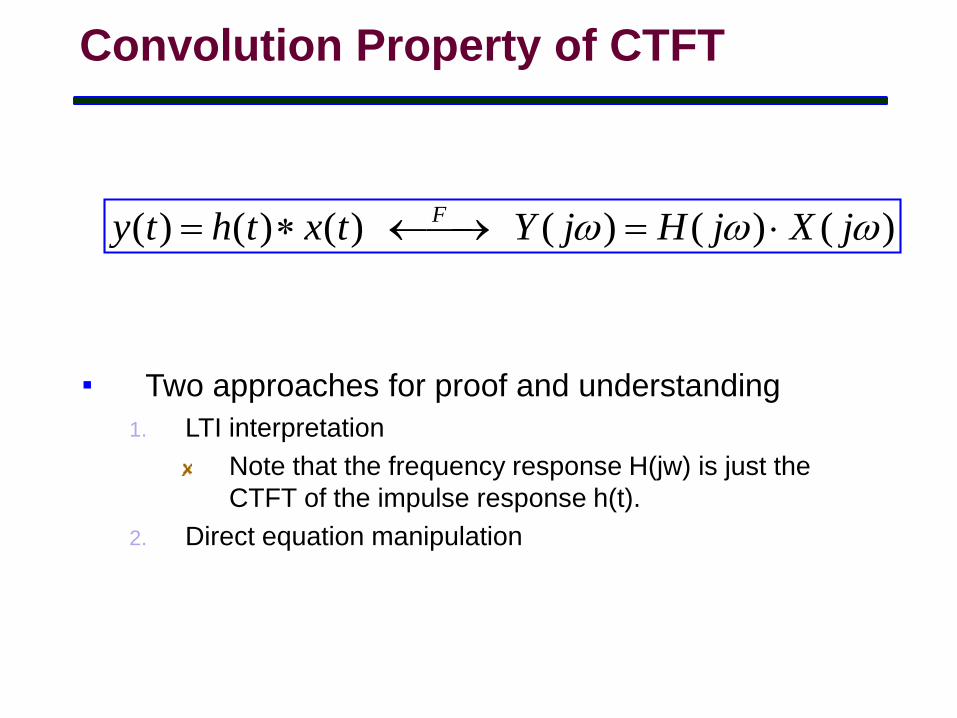
( ) ( ) ( ) ( ) ( ) ( )Fy t h t x t Y j H j X j
Two approaches for proof and understanding
1. LTI interpretation
Note that the frequency response H(jw) is just the
CTFT of the impulse response h(t).
2. Direct equation manipulation

Lowpass Filter
0
0 0
0
0,
( ) ( ),
0,
Y j X j
Convolution Property of CTFT
H(j)
-0 0
1X(j) Y(j)
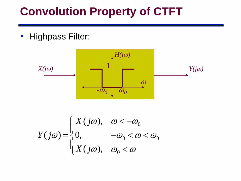
Highpass Filter:
0
0 0
0
( ),
( ) 0,
( ),
X j
Y j
X j
Convolution Property of CTFT
H(j)
-0 0
1X(j) Y(j)

Bandpass Filter:
1 2
1 2
( ),
( ) ( ),
0, otherwise
X j
Y j X j
Convolution Property of CTFT
H(j)
-2 -1 1 2
1X(j) Y(j)

Examples

CTFT Table

CTFT Table

CTFT Table
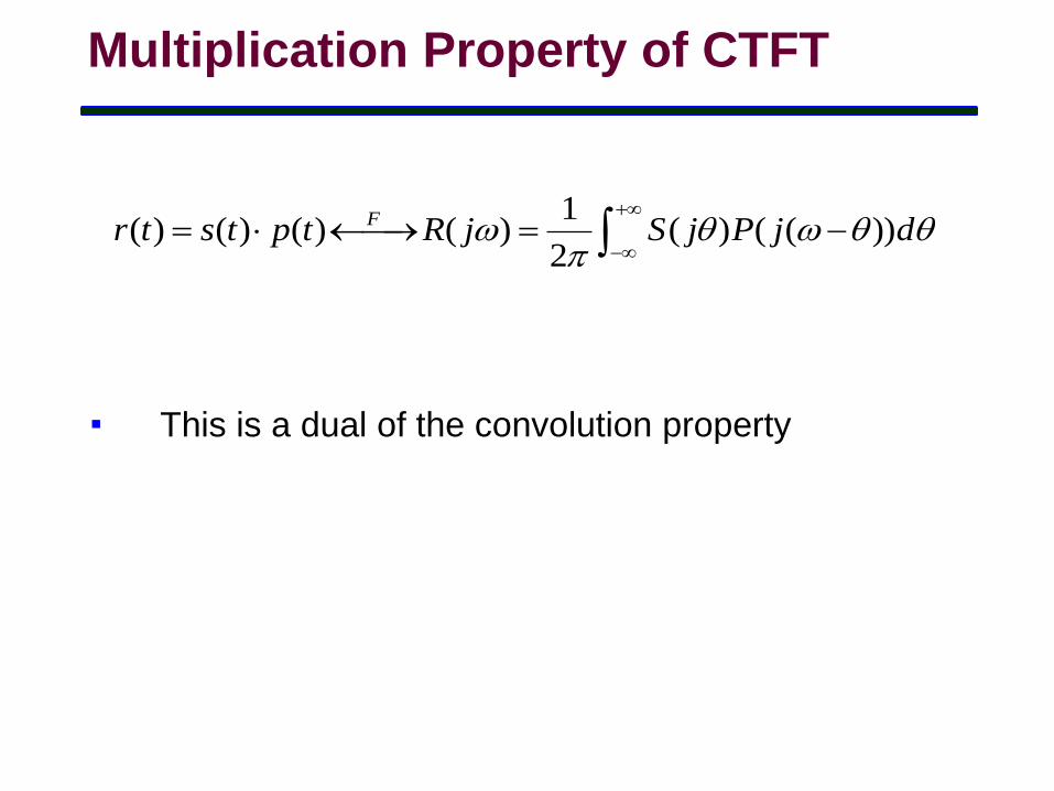
Multiplication Property of CTFT
1( ) ( ) ( ) ( ) ( ) ( ( ))
2
Fr t s t p t R j S j P j d
This is a dual of the convolution property

- 00
A/2
G(j)
modulation
FT of p(t)=cos0t
- 00
P(j)
FT of r(t)
A
R(j)
g(t)p(t) Q(j) F
A/2
-200 20
A/4
Original signal is recovered after a low-pass filter
g(t) = r(t)p(t)
demodulation
Multiplication Property of CTFT
Idea of AM (amplitude modulation)
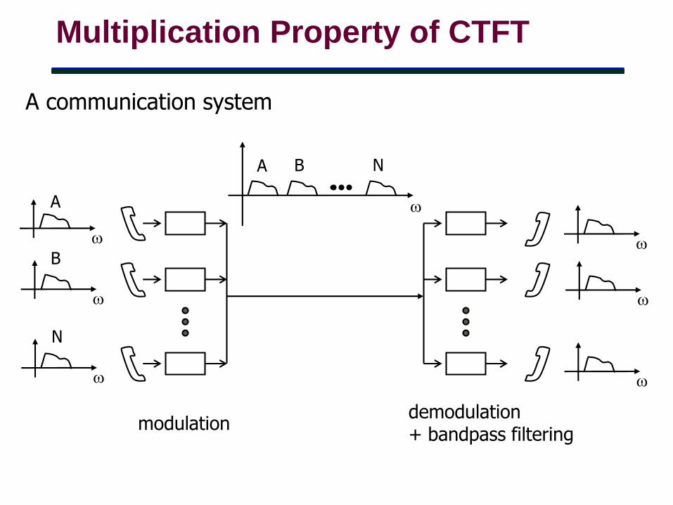
Multiplication Property of CTFT
A communication system
modulation
A
B
N
A B N
demodulation+ bandpass filtering

Causal LTI Systems Described
by Differential Equations

Linear Constant-Coefficient Differential
Equations
The DE describes the relation between the input x(t)
and the output y(t) implicitly
In this course, we are interested in DEs that
describe causal LTI systems
Therefore, we assume the initial rest condition
which also implies
M
kk
k
k
N
kk
k
kdt
txdb
dt
tyda
00
)()(
0 0If ( ) 0 for , then ( ) 0 forx t t t y t t t
1
0 00 1
( ) ( )( ) 0
N
N
dy t d y ty t
dt dt

Frequency Response
What is the frequency response H(jw) of the
following system?
It is given by
M
kk
k
k
N
kk
k
kdt
txdb
dt
tyda
00
)()(
0
0
( )( )
( )
M k
kk
N k
kk
b jH j
a j

Example
2
2
( ) ( ) ( )4 3 ( ) 2 ( ),
( ) ( ).t
d y t dy t dx ty t x t
dt dt dt
x t e u t
2
2
1 1 14 2 4
2
( ) ( ) ( )
2 1
( ) 4( ) 3 1
2
( 1) ( 3)
1 ( 1) 3
Y j H j X j
j
j j j
j
j j
j j j
31 1 1( ) ( )
4 2 4
t t ty t e te e u t
Q)
A)
Recommended


![3. Continuous and discrete time Fourier series - UPT · Continuous and discrete time Fourier series ... The discrete time signal x[n] ... following signals: Solution. a) 9. 10](https://img.dokumen.tips/doc/110x75/5b89429c7f8b9a655f8bce4f/3-continuous-and-discrete-time-fourier-series-continuous-and-discrete-time.jpg)


