Short and Long-run Determinants of Sovereign Debt Credit Ratings*
António Afonso, $ # Pedro Gomes,+ and Philipp Rother #
Abstract We study the determinants of sovereign debt credit ratings using rating notations from the three main international rating agencies, for the period 1995-2005. Using linear methods and ordered response models we employ a new specification that allows us to distinguish between short and long-run effects, on a country’s rating, of several macroeconomic and fiscal explanatory variables. The results point to a good performance of the estimated models, across agencies and time, as well as a good overall prediction power. Changes in GDP per capita, GDP growth, government debt, government balance have a short-run impact on a country’s credit rating, while government effectiveness, external debt, foreign reserves and default history are important long-run determinants. JEL: C23; C25; E44; F30; G15 Keywords: credit ratings; sovereign debt; rating agencies; panel data; random effects ordered probit
* We are grateful to Fitch Ratings, Moody’s, and Standard & Poor’s for providing us historical sovereign rating data, to Renate Dreiskena for help with the data, to Vassilis Hajivassiliou and Philip Vermeulen for helpful clarifications, to Moritz Kraemer, Guido Wolswijk, and to participants at ECB and ISEG/UTL seminars, at the 2007 North American Summer Meeting of the Econometric Society, at the Money, Macro and Finance Research Group 39th Annual Conference and at the XLI Euro Working Group on Financial Modelling conference for useful comments. The opinions expressed herein are those of the authors and do not necessarily reflect those of the the ECB or the Eurosystem. $ ISEG/UTLisbon - Technical University of Lisbon, Department of Economics; UECE – Research Unit on Complexity and Economics, R. Miguel Lupi 20, 1249-078 Lisbon, Portugal. UECE is supported by FCT (Fundação para a Ciência e a Tecnologia, Portugal), email: [email protected]. # European Central Bank, Directorate General Economics, Kaiserstraße 29, D-60311 Frankfurt am Main, Germany, emails: [email protected]; [email protected]. + London School of Economics & Political Science; STICERD – Suntory and Toyota International Centres for Economics and Related Disciplines, Houghton Street, London WC2A 2AE, email: [email protected]. The author would like to thank the Fiscal Policies Division of the ECB for its hospitality and aknowledge financial support of FCT.

2
1. Introduction
Sovereign credit ratings are a condensed assessment of a government’s ability and willingness
to repay its public debt on time, both in principal and in interests. In this, they are forward-
looking qualitative measures of the probability of default put forward by rating agencies.
Sovereign credit ratings are particularly relevant for international financial markets, economic
agents and governments. Indeed, they are important in three ways. First, sovereign ratings are
a key determinant of the interest rates a country faces in the international financial market and
therefore of its borrowing costs. Second, the sovereign rating may have a constraining impact
on the ratings assigned to domestic banks or companies. Third, some institutional investors
have lower bounds for the risk they can assume in their investments and they will choose their
bond portfolio composition taking into account the credit risk perceived via the rating
notations1. Therefore, it is important both for governments and for financial markets to
understand what factors rating agencies put more emphasis on when attributing a rating score.
In this paper we perform an empirical analysis of foreign currency sovereign debt ratings,
using rating data from the three main international rating agencies: Fitch Ratings, Moody’s,
and Standard & Poor’s. We have compiled a comprehensive panel data set on sovereign debt
ratings, macroeconomic data, and qualitative variables for a wide range of countries starting in
1995. In this context, the use of panel data is appealing because it allows examining not only
how the agencies attribute a rating, but also how they decide on upgrades and downgrades.
Our main contributions to the existing literature are both the innovation of the econometric
estimation procedure and the specification used. Indeed, the fact that a country’s rating does
not have much variation across time raises some econometric problems. While fixed effects
estimations are uninformative as the country dummy captures the average rating, random 1 For instance, the European Central Bank when conducting open market operations can only take as collateral bonds that have at least a single A rating attributed by at least one rating agency.

3
effects estimations will also be inadequate due to the correlation between the country specific
error and the regressors. We salvage the random effects approach by means of modelling the
country specific error, which in practical terms implies adding time-averages of the
explanatory variables as additional time-invariant regressors. This setting will allow us to
make a distinction between short and long-run effects of a variable on the sovereign rating.
This distinction can be very important for policy purposes because it can inform the
governments what they can do to improve their rating in the short-run.
Regarding the empirical modelling strategy, we follow the two main strands in the literature.
We make use of linear regression methods on a linear transformation of the ratings and we
also estimate our specifications using both ordered probit and random effects ordered probit
methods. The latter is the best procedure for panel data as it considers the existence of an
additional normally distributed cross-section error. This approach allows both to determine the
cut-off points throughout the rating scale as well as to test whether a linear quantitative
transformation of the ratings is, in fact, a good approximation. Furthermore, we perform
robustness check by allowing for a sub-period analysis and for a differentiated high and low
rating analysis.
The results show that in particular four core variables have a consistent short run impact on
sovereign ratings. These are the level of GDP per capita, real GDP growth, the public debt
level and government balance. Government effectiveness, as well as the level of external debt
and external reserves are important long-run determinants of sovereign ratings. A dummy
reflecting past sovereign defaults is also found significant. It is noteworthy that, using our
methodology, fiscal variables are more important determinants than found in the previous
literature.

4
The paper is organised as follows. In Section Two we give an overview of the rating systems
and review the relevant related literature. Section Three explains our methodological choices,
specifically regarding the econometric approaches employed. In Section Four we report on the
empirical analysis, notably in terms of the estimation and prediction results, as well as some
country specific analysis. Section Five summarises the paper’s main findings.
2. Rating systems and literature
Sovereign ratings are assessments of the relative likelihood of default. The rating agencies
analyse a wide range of elements, from solvency factors that affect the capacity to repay the
debt, to socio-political factors that might affect the willingness to pay of the borrower, and
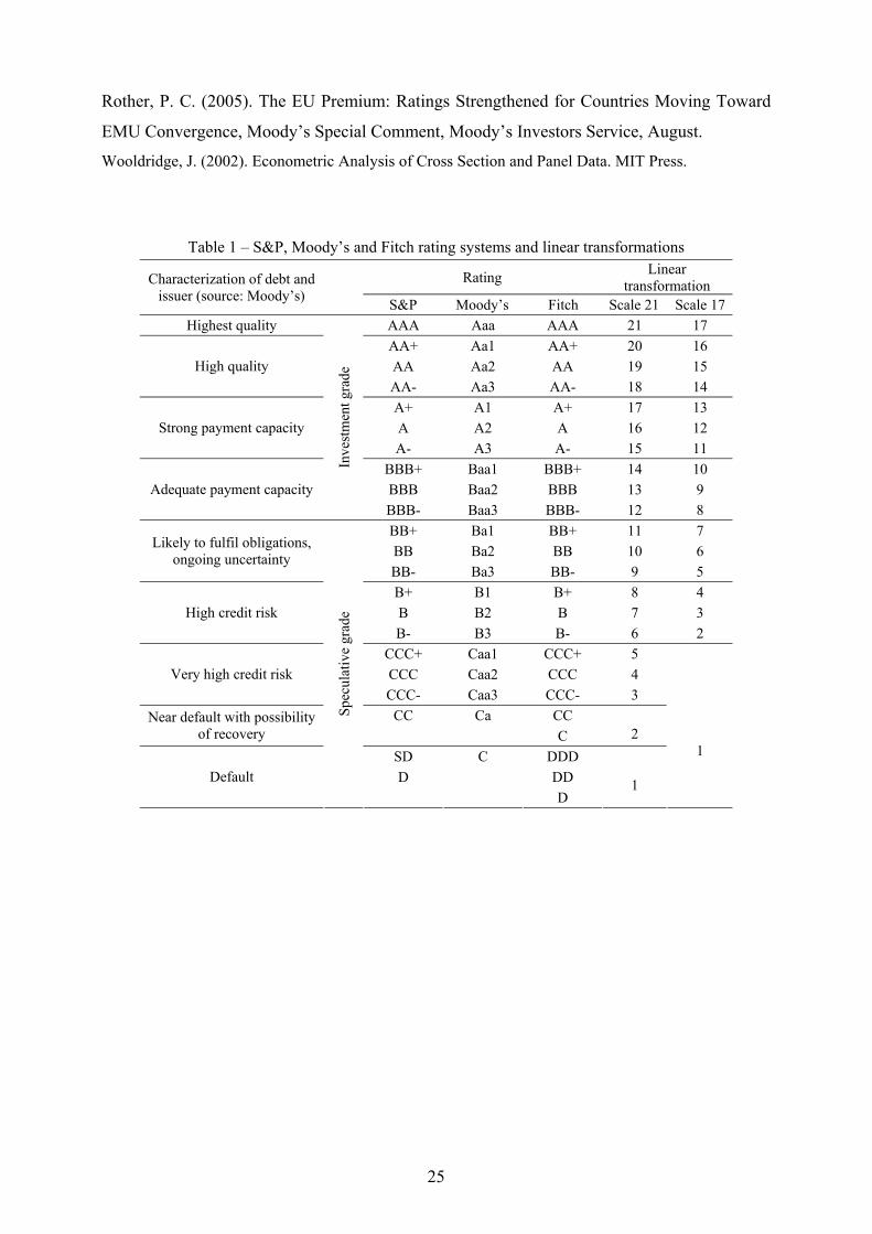
assess the risk of default using a code. Although these agencies do not use the same qualitative
codes, in general, there is a correspondence between each agency rating level as shown in
Table 1.
[Table 1]
A first study on the determinants of sovereign ratings by Cantor and Packer (1996) concluded
that the ratings can be largely explained by a small set of variables namely: per capita income,
GDP growth, inflation, external debt, level of economic development, and default history.
Further studies incorporated more variables, for instance, macroeconomic performance
variables like the unemployment rate or the investment-to-GDP ratio (Bissoondoyal-Bheenick,
2005). In papers focussing on the study of currency crises several external indicators such as
foreign reserves, current account balance, exports or terms of trade seem to play an important
role (Monfort and Mulder, 2000). Moreover, indicators of how the government conducts its
fiscal policy, budget balance and government debt can also be relevant, as well as variables
that assess political risk, like corruption or social indexes (Depken et al., 2007).

5
Regarding the econometric approach, there are two major strands in the literature. The first
uses linear regression methods on a numerical representation of the ratings. The early study by
Cantor and Packer, applies OLS regressions to a linear representation of the ratings, on a cross
section of 45 countries. This methodology was also pursued by Afonso (2003) and Butler and
Fauver (2006). Using OLS analysis on a numerical representation of the ratings is quite simple
and allows for a straightforward generalization to panel data by doing fixed or random effects
estimation (Mora, 2006; Monfort and Mulder, 2000).
Although estimating the determinants of ratings using these approaches has in general a good
fit and a good predictive power it faces some critiques. As ratings are a qualitative ordinal
measure, using traditional estimation techniques on a linear representation of the ratings is not
the most adequate framework of estimation. First, it implies the assumption that the difference
between two rating categories is equal for any two adjacent categories, which would need to
be tested. Furthermore, even if this assumption was true, because of the presence of elements
in the top and bottom category, the estimates are biased, even in big samples.
To overcome this critique another strand of the literature uses ordered response models. These
methods will themselves determine the size of the differences between each category. For
example, this procedure was used by Hu et al. (2002), Bissoondoyal-Bheenick (2005),
Bissoondoyal-Bheenick et al. (2006) and Depken et al. (2007). Although this should be
considered the preferred estimation procedure it is not entirely satisfying. The crucial point is
that the ordered probit asymptotic properties do not generalise for a small sample, so if we
estimate the determinants of the ratings using a cross-section of countries, we would have too
few observations. It is therefore imperative to try to maximize the number of observation by
using panel data, but when doing so, one has to be careful. Indeed, the generalization of
ordered probit to panel data is not completely straightforward, due to the existence of a

6
country specific effect. Furthermore, within this framework, the need to have many
observations makes it harder to perform robustness analysis by, for instance, partitioning the
sample.
3. Methodology
3.1. Linear regression framework
A possible starting point for our linear panel model would follow Monfort and Mulder (2000)
and Mora (2006), generalizing a cross section specification to panel data,
it it i i itR X Z aβ λ µ= + + + , (1)
where we have: R – quantitative variable, obtained by a linear or by a non-linear
transformation; Xit is a vector containing time varying variables that includes the time-varying
explanatory variables described above and Zi is a vector of time invariant variables that
include regional dummies.
In (1) the index i (i=1,…,N) denotes the country, the index t (t=1,…,T) indicates the period and
ai stands for the individual effects for each country i (that can either be modelled as a error
term or as N dummies to be estimated). Additionally, it is assumed that the disturbances µit are
independent across countries and across time.
There are three ways to estimate this equation: pooled OLS, fixed effects or random effects
estimation. Under standard conditions all estimators are consistent and the ranking of the three
methods in terms of efficiency is clear: a random effects approach is preferable to the fixed
effects, which is preferable to pooled OLS. What we mean by standard conditions is whether
or not the country specific error is uncorrelated with the regressors E(ai| Xit, Zi)=0. If this is the
case one should opt for the random effects estimation, while if this condition does not hold,

7
both the pooled OLS and the random effects estimation give inconsistent estimates and fixed
effects estimation is preferable.
In our case, it seems more natural that the country specific effect is correlated with the
regressors.2 Given this scenario one should be tempted to say that the “fixed effects
estimation” is the best strategy, but that has a problem. Because there is not much variation of
a countries rating over time, the country dummies included in the regression will capture the
country’s average rating, while all the other variables will only capture movements in the
ratings across time. This means that, although statistically correct, a regression by fixed effects
would be seriously stripped of meaning.
There are two ways of rescuing a random effects approach under correlation between the
country specific error and the regressors. One is to do the Hausman-Taylor IV estimation but
for that we would have to come up with possible instruments that are not correlated with ai,
which does not seem an easy task. In this paper we will opt for a different approach that
consists on modelling the error term ai. This approach, described in Wooldridge (2002), is
usually applied when estimating non-linear models, as IV estimation proves to be a Herculean
task but. As we shall see, the application to our case is quite successful. The idea is to give an
explicit expression for the correlation between the error and the regressors, stating that the
expected value of the country specific error is a linear combination of time-averages of the
regressors iX . This follows Hajivassiliou and Ioannides (2007).
( | , ) ii it iE a X Z Xη= . (2)
If we modify our initial equation (1), with ti ia Xη ε= + we get
2 In several studies, like Depken et al. (2007) and Mora (2006), the random effects estimator is rejected by the Hausman test. We confirm this result by doing some exploratory regressions. We estimated equation (1) using random effects and performed the Hausman test; the Chi-Square statistic is in fact very high, and the null hypothesis of no correlation is rejected with p-value of 0.000.

8
iXit it i i itR X Zβ λ η ε µ= + + + + , (3)
where iε is an error term by definition uncorrelated with the regressors. In practical terms, we
eliminate the problem by including a time-average of the explanatory variables as additional
time-invariant regressors. We can rewrite (3) as:
( X ) ( )Xi iit it i i itR X Zβ η β λ ε µ= − + + + + + . (4)
This expression is quite intuitive.δ η β= + can be interpreted as a long-term effect (e. g. if a
country has a permanent high inflation what is the respective effect on the rating), while β is a
short-term effect (e. g. if a country manages to reduce inflation this year by one point what
would be the effect in the rating). This intuitive distinction is useful for policy purposes as it
can tell what a country can do to improve its rating in the short to medium-term. Alternatively,
we can interpret δ as the coefficient of the cross-country determinants of the credit rating. We
will estimate equation (4) by random effects. The way we modelled the error term can be
considered successful if the coefficients η are significant and if the Hausman test indicates no
correlation between the regressors and the new error term.
3.2. Ordered response framework
Alternatively we estimate the determinants of sovereign debt ratings in a limited dependent
variable framework. As we mentioned before, the ordered probit is a natural approach for this
type of problem, because the rating is a discrete variable and reflects an order in terms of
probability of default. The setting is the following. Each rating agency makes a continuous
evaluation of a country’s credit-worthiness, embodied in an unobserved latent variable R*.
This latent variable has a linear form and depends on the same set of variables as before,
* ( X ) Xi iit it i i itR X Zβ δ λ ε µ= − + + + + . (5)

9
Because there is a limited number of rating categories, the rating agencies will have several
cut-off points that draw up the boundaries of each rating category. The final rating will then be
given by
*16
*16 15
*15 14
*1
( ) ( 1)
( 2)
( 1)
it
it
it it
it
AAA Aaa if R cAA Aa if c R c
R AA Aa if c R c
CCC Caa if c R
⎧ >⎪ + > >⎪⎪= > >⎨⎪⎪⎪< + >⎩
M. (6)
The parameters of equation (5) and (6), notably β, δ, λ and the cut-off points c1 to c16 are
estimated using maximum likelihood. Since we are working in a panel data setting, the
generalization of ordered probit is not straightforward, because instead of having one error
term, we now have two. Wooldridge (2002) describes two approaches to estimate this model.
One “quick and dirty” possibility is to assume we only have one error term that is serially
correlated within countries. Under that assumption one can do the normal ordered probit
estimation but a robust variance-covariance matrix estimator is needed to account for the serial
correlation. The second possibility is the random effects ordered probit model, which
considers both errors εi and µit to be normally distributed, and the maximization of the log-
likelihood is done accordingly. This second approach should be considered the best one, but it
has as a drawback the quite cumbersome calculations involved.3
3.3. Explanatory variables
Building on the evidence provided by the existing literature, we identify a set of main
macroeconomic and qualitative variables that may determine sovereign ratings, which we can
aggregate in four main areas.
Macroeconomic variables
3 In STATA this procedure was created by Rabe-Hesketh et al. (2000) and substantially improved by Frechette (2001a, 2001b) Wewill use such procedures in our calculations.

10
GDP per capita – positive impact on rating: more developed economies are expected to have
more stable institutions to prevent government over-borrowing and to be less vulnerable to
exogenous shocks.
Real GDP growth – positive impact: higher real growth strengthens the government’s ability
to repay outstanding obligations.
Unemployment – negative impact: a country with lower unemployment tends to have more
flexible labour markets making it less vulnerable to changes in the economic environment. In
addition, lower unemployment reduces the fiscal burden of unemployment and social benefits
while broadening the base for labour taxation.
Inflation – uncertain impact: on the one hand, it reduces the real stock of outstanding
government debt in domestic currency, leaving overall more resources for the coverage of
foreign debt obligations. On the other hand, it is symptomatic of problems at the
macroeconomic policy level, especially if caused by monetary financing of deficits.
Government variables
Government debt – negative impact: a higher stock of outstanding government debt implies a
higher interest burden and should correspond to a higher risk of default.
Fiscal balance – positive impact: large fiscal deficits absorb domestic savings and also suggest
macroeconomic disequilibria, negatively affecting the rating level. Persistent deficits may
signal problems with the institutional environment for policy makers.
Government effectiveness – positive impact: high quality of public service delivery,
competence of bureaucracy and lower corruption should impinge positively of the ability to
service debt obligations.
External variables
External debt – negative impact: the higher the overall economy’s external indebtedness, the
higher becomes the risk for additional fiscal burdens, either directly due to a sell-off of foreign
government debt or indirectly due to the need to support over-indebted domestic borrowers.

11
Foreign reserves – positive impact: higher (official) foreign reserves should shield the
government from having to default on its foreign currency obligations.
Current account balance – uncertain impact: a higher current account deficit could signal an
economy’s tendency to over-consume, undermining long-term sustainability. Alternatively, it
could reflect rapid accumulation of fixed investment, which should lead to higher growth and
improved sustainability over the medium term.
Other variables
Default history – negative impact: past sovereign defaults may indicate a great acceptance of
reducing the outstanding debt burden via a default. The effect is modelled by a dummy
variable indicating the past occurrence of a default and by a variable measuring the number of
years since the last default. This variable measures the recovery of credibility after a default
and can be expected to influence positively the rating score.
European Union – positive impact: countries that join the European Union improve their
credibility as their economic policy is restricted and monitored by other member states.
Regional dummies – uncertain impact: some groups of countries of the same geographical
location may have common characteristics that affect their rating.
4. Empirical analysis
4.1. Data
We build a ratings database with sovereign foreign currency rating attributed by the three main
rating agencies Standard & Poor’s, Moody’s and Fitch Ratings. For the rating notations we
covered a period from 1970 to 2005. The rating of a particular year is the rating that was
attributed at 31st of December of that year4. In 2005 there are 130 countries with a rating,
though only 78 have a rating attributed by all three agencies. For the linear panel we grouped
the ratings in 17 categories, by putting together the few observations below B- (see Table 1).
4 The full historical rating dataset that we compiled, including foreign and local currency ratings as well as credit rating outlooks, is available from the authors on request.

12
Given the data availability of the explanatory variables our estimations only cover the period
from 1995 to 2005. Fiscal balance, current account and government debt are in percentage of
GDP, foreign reserves enter as percentage of imports and external debt as percentage of
exports. The variables inflation, unemployment, GDP growth, fiscal balance and current
account enter as a 3-year average, reflecting the agencies’ approach to take out the effect of
the business cycle when deciding on a sovereign rating. The external debt variable was taken
from the World Bank and is only available for non-industrial countries, so for industrial
countries it was attributed the value 0, which is equivalent to having a multiplicative dummy.
As for the dummy variable for European Union, we consider that the rating agencies
anticipated the EU accession. Thus we tested the contemporaneous variable as well as up to
three leads. We find that for Moody’s and S&P the variable enters with two leads, while for
Fitch we find no anticipation of EU accession. Regarding the regional dummies, only the
dummies for Industrialised countries and for Latin America and Caribbean countries were
significant. Overall we have an unbalanced panel with 66 countries for Moody’s, 65 for S&P
and 58 for Fitch, with an average 8 yearly observations per country.5
4.2. Linear panel results
Full sample
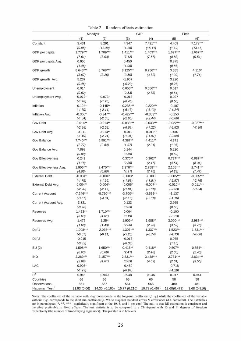
In view of the analytical considerations above we focus the discussion on the random effects
estimations (see Table 2). This is supported by the Hausmann tests reported at the end of the
table that points to the acceptability of the random effects approach.6
[Table 2]
5 See Afonso et al. (2007) for a full list of variables used in the estimations as well as their specification and data sources, notably IMF World Economic Outlook, World Bank Aggregate Governance Indicator and Jaimovich, Panizza (2006) for government debt. 6 We also estimated the model using OLS and fixed effects. Results are not reported for space sake, but can be found in Afonso et al. (2007)

13
We report the results of two models for each rating agency, the unrestricted and the restricted
model. While the unrestricted model incorporates all variables discussed above, the restricted
model contains only the variables which were found to have a statistically significant impact.
Although the sequence of excluding individual variables in moving from the unrestricted to
the restricted regression can have an impact on the final specfication, the restricted models
presented in Table 2 are quite robust to alternative exclusion procedures. As can be seen from
the statistics reported at the end of each table, the explanatory power of the models is very
high with R-square values around 95 per cent and it remains almost constant moving from the
unrestricted to the restricted versions. In addition, the variables found to be significant in the
unrestricted model generally remain significant with the same sign in the restricted version.
Moreover, we can also assess how successful and important our specification is. First, in most
of the cases, the short and long–run coefficients of the explanatory variables are quite
different, which implies that if we did not include the additional regressors we would be
mispecifying the model.7 Second, the models pass the Hausman test, which suggests that the
country specific error is now uncorrelated with the regressors. In other words, if we do not
include the time averages the model would suffer from an omitted variables proble, which
would make OLS and random effects inconsistent.
The restricted models (columns 2, 4, and 6 in Table 2) reveal a homogenous set of explanatory
variables across agencies. On the real side, the short-run coefficients of GDP per capita and
GDP growth rates turn out significant for all three companies, but do not seem to have a long
run effect. In terms of magnitude, an increase of 2 percentage points of GDP growth improves
7 We perform the formal significance test by estimating equation (3) and testing directly the coefficients of the time averages of the explanatory variables. Average per capita GDP and government effectiveness are allways significant at 5% for all agencies. In addition, average unemployment is significant for Moody´s, average government debt is significant for S&P and the average reserves-to-imports is significant for S&P and Fitch. If we exclude all the time invariant regressors the remaining coefficients change slightly and some lose their significance. None of the models without the additional variables pass the Hausman test.

14
the rating by around 0.17 notches for Moody’s and S&P, while an increase of 6 percent of
GDP per capita improves the rating by around 0.1 notch.
Regarding the fiscal variables, the coefficient of the government debt-to-GDP ratio as a
difference from the average is significant for all three agencies. According to our results, S&P
and Fitch seem to put slightly more emphasis on this variable than the other two agencies: a 10
percentage point decline in the government debtto-GDP ratio improves the rating by 0.3
notches (the improvement for Moody’s is 0.15 notches). On the other hand, Moody’s puts
more emphasis on the the government balance: a 3 percentage point decrease in the deficit
ratio raises Moody’s rating by 0.2 and by 0.1 in the other two agencies. Given their
interdependence one can not see these effects in isolation but rather together, which implies a
high overall effect of fiscal policies on the ratings. Finally, government effectiveness indicator
is an important determinant of the rating in the long run. On average, an improvement of 1
point in the World Bank indicator translates into an improvement of 2 notches across all
specifications. Additionally, it is possible to observe that the cross-country difference between
the 10th and 90th percentile of the average government effectiveness indicator between
countries is 2.5 points. This means that government effectiveness indicator is capturing
elements that account for 5 notches difference between them.
With respect to external variables, the external debt to exports ratio and the level of reserves–
to-imports ratio are found to be significant across agencies. Increases in external debt drive the
rating down in the short and long-run. The difference between the 10th and 90th percentile of
the cross-country average external debt ratio is around 300, which corresponds to a cross-
country difference of 3 notches for Fitch, 2 notches for S&P, and 1.2 notches for Moody’s.
External reserves ares significantly positive, in the long-run for S&P and Fitch and in the
short-run for Moody’s. The difference between the 10th and 90th percentile of the average

15
reserves to import ratio is 0.4 which implies that the reserves account for a 1.2 notch cross-
country difference for Fitch and a 0.8 notches for S&P. The current account balance has a
negative impact in the short run. A current account deficit seems to be an indicator for the
willingness of foreigners to cover the current account gap through loans and foreign
investment. In this situation, a higher current account deficit is associated with either higher
credit-worthiness or good economic prospects of the economy and consequently a higher
sovereign rating.
EU and industrial country dummies are also significant for all agencies. If a country
previously defaulted on its debt, it is penalized by the agencies by 1 to 2 nothes and this effect
does not seem to disapear with time.
Beyond this set of core variables, the agencies appear to employ a limited number of
additional variables. For Fitch the analysis finds the smallest set of additional variables,
comprising government effectiveness as a deviation from the average and foreign currency
reserves also in terms of its short-run deviation. By contrast, the analysis finds more
significant explanatory variables for Moody’s and Standard and Poor’s, with a large degree of
homogeneity between these two agencies. In particular, on the real side inflation is found to
have a significantly negative impact, although with a relative small magnitude. Finally, the
impact of the unemployment on the rating ilustrates the importance of distinguishing short and
long run impacts. While the average (stuctural) level of unemployment is found to have a
significant negative impact on the rating by Moody’s, the short-run deviation from the average
enters positively and significantly in the S&P model. Unemployment in the short run can be
driven by re-adjustments of economic activity that might improve economic performance in
the future. Also, structural reforms that raise unemployment in the short run but improve fiscal

16
sustainability or economic prospects in the long run could provide an explanation for this latter
finding.
Differentiation across sub-periods and ratings levels8
The separation of the overall sample into different sub-samples allows to assess broadly the
robustness of the empirical models.9 In particular, the results for the sub-periods 1996-2000
and 2001-2005 are generally in line with those for the full estimation period, although the
significance levels of the individual coefficients are reduced. In particular, the core variables
identified above enter the models for the sub-periods with the correct sign and generally
significantly with a comparable order of magnitude. The most noteworthy element is that for
the early sub-period, 1996-2000, the current account balance was more important, while
external reserves were somewhat more important in the later period, 2001-2005 (for Moody’s
and S&P).
As a further test of the robustness of the results, the sample was split into two groups
according to the ratings level: regressions were run separately for high-rated countries with
grades BBB+ and below and those above this grade.10 The results for the separate regressions
according to ratings levels again confirm the overall results from the full sample. A few
elements are interesting to mention: low rating levels are more affected by external debt and
external reserves while inflation plays a bigger role for high rating levels. The magnitude of
the short-run coefficient of inflation is much higher for the high ratings group, where an
increase of 5 percentage points in inflation reduce the rating by 0.2 notches.
8 We performed additional analysis from different perspectives. For instance, we used the information on credit rating outlooks but no relevant improvement on the fit of the models occurred. In addition, we assessed whether different exchange rate regimes added information to the rating determination, estimated the model with the average rating of the three agencies, and also pooled the data for the three agencies, but the results where quite similar. 9 Results not reported for space sake, but available in Afonso et al. (2007). 10 The choice of the threshold reflects practical considerations. While market participants generally divide bond issuers into investment-grade and non-investment grade at the threshold of BBB-, this threshold would result in a relatively small number of observations for low ratings making inference problematic.

17
4.4. Ordered probit results
In view of the discussion of econometric issues above, ordered probit models should give
additional insight into the determinants of sovereign ratings. In particular, this method allows
to relax the rigid assumption on the shape of the ratings schedule. Instead it generates
estimates of the threshold values between rating notches allowing an assessment of the shape
of the ratings curve. Given the data requirements, the method was only applied to the full
sample, which appears appropriate in view of the overall robustness of the empirical results to
the use of sub-samples.
The results from the ordered probit estimations validate the findings highlighted above (see
Table 3 for the random effects ordered probit). The core variables identified in the linear
regressions also show up with the correct sign. In addition, the ordered probit models suggest
the significance of somewhat more explanatory variables, particularly for Fitch. At the same
time, in the area of external variables, reserves do not show up significantly for S&P and Fitch
in the restricted specifications. Finally, for the current account variable, the restricted
specification for Moody’s shows a negative sign for deviations from the long-term average,
but a positive sign for the average, and similar sign switches appear also in some instances for
the other agencies. This result confirms our priors. In the short run, higher current account
deficits are associated with either higher credit-worthiness or good economic prospects of the
economy but if the countries run permanent current account deficits than it affect negativelly
their ratings.
[Table 3]
The estimated threshold coefficients reported in the second part of Table 3 suggest that the
linear specification assumed for the panel regression above is broadly acceptable. For instance,
the results show that for all three agencies the thresholds between rating notches are broadly

18
equally distributed across the ratings range. In other words, the distance for a country to move
e.g. from B– to B is roughly equal to that for moving from AA to AA+. Nevertheless, the
econometric tests at the bottom of the tables reveal additional insights. For the restricted model
of Moody’s, the test does not reject the null hypothesis of equal distances between thresholds,
but the significance level is close to 10 per cent. Indeed the estimated thresholds point to a
relatively large jump between the ratings for BBB– and BBB. This suggests that countries
close to the non-investment grade rating are given a wider range before they actually cross that
threshold. For Fitch, the hypothesis of equal distances is strongly rejected as the thresholds for
higher ratings are further apart than those of the lower ratings. In this case the kink lies at the
A rating. For S&P, different distances are found throughout the ratings scale and it appears
that for lower ratings the relative distance between thresholds of S&P coincides with that of
Moody’s. However, above the investment grade limit, the distances between thresholds at first
decline and then increase, resulting in a slightly curved ratings schedule that makes the
transition to the highest grades most difficult.
4.5. Prediction analysis
Our prediction analysis will focus on two elements: the prediction for the rating of each
individual observation in the sample, as well as the prediction of movements in the ratings
through time. For the random effects estimations we can have two predictions, with or without
the country specific effect, εi, and we can write the corresponding estimated versions of (4) as:
ˆ ˆ ˆˆ ˆ( X ) Xi iit it i iR X Zβ δ λ ε= − + + + , (7a)
ˆ ˆ ˆ( X ) Xi iit it iR X Zβ δ λ= − + +% . (7b)
We can then estimate each country specific effect by taking the time average of the estimated
residual for each country. As a result we can include or exclude this additional information
that comes out of the estimation. We also present the predicting results using OLS estimation.
For the linear models we compute the fitted value and then rounded it to the closest integer

19
between 1 and 17. The prediction with both ordered probit and the random effects ordered
probit was done by fitting the value of the latent variable, setting the error term to zero, and
then match it up to the cut-off points do determine the predicted rating. Table 4 presents an
overall summary of the prediction errors, for the three agencies and for the several methods
using the respective restricted specifications.
[Table 4]
The first conclusion is that the random effects model including the estimated country effect is
the method with the best fit. On average for the three agencies, it correctly predicts 70 per cent
of all observations and more than 95 per cent of the predicted ratings lie within one notch (99
per cent within two notches). This is expected, as the country errors capture factors like
political risk, geopolitical uncertainty and social tensions that are likely to systematically
affect the ratings, therefore, such term acts like a correction for these factors.
This additional information cropping up from the random effects estimation with the country
specific effect can be very useful if we want to work with countries that belong to our sample.
But if we want to make out of sample predictions we will not have this information. In that
case, only the random effects estimation excluding the country error is comparable to the OLS
specification, to the ordered probit and to the random effects ordered probit. We can see that in
general both ordered probit and random effects ordered probit have a better fit than the pooled
OLS and random effects for all three agencies, though not as clearly for Fitch. Overall, the
simple ordered probit seems the best method as far as prediction in levels is concerned as it
predicts correctly around 45 per cent of all observations and more then 80 per cent within one
notch.
Let’s now turn to how the models perform in predicting changes in ratings. Table 5 presents
the total number of sample upgrades (downgrades), the predicted number of upgrades

20
(downgrades) and the number of upgrades (downgrades) that where correctly predicted by the
several models. It is worthwhile to highlight that over the sample period, on average, there was
a change of rating every six years for Moody’s and every five years for S&P and Fitch. Of
these changes a country was twice more likely to be upgraded than downgraded.11
[Table 5]
Roughly the models correctly predict between one third and one half of both upgrades and
downgrades. This is quite satisfactory for two reasons: first, the rating agencies also have a
forward looking behaviour that is absent from our models and second, other qualitative factors
not captured in our variables may play an important role.
The most noticeable difference between the models is not the number of corrected predicted
changes but the total number of predicted changes. In fact, the ordered probit and random
effects ordered probit predict significantly more changes than the OLS and random effects
counterparts. For instance, for S&P, while both OLS and random effects predict around 79
upgrades and 50 downgrades, the ordered probit model predicts 102 upgrades and 64
downgrades. This gives strength to the idea that rating agencies smooth the ratings, along the
lines discussed, for instance, in Altman and Rijken (2004). It also suggests that linear methods
might be better in capturing the inertia of rating agencies than ordered response models.
4.6. Examples of specific country analysis
In Table 6 we show, as an example, the rating for some European countries and some
emerging markets both in 1998 and 2005. Then, we use the estimated short-run coefficients of
the random effects ordered probit together with the values for the relevant variables to
disaggregate the overall prediction change in the rating of each agency into the contributions
11 This analysis is, in a way, limited as it does not capture upgrades/downgrades across multiple grades or multiple upgrades/downgrades within a year. Although this could be important to analyse particular cases, such as, for instance, currency crises, the cases of multiple upgades/downgrades are relatively small compared to the full sample.

21
of the different blocks of explanatory variables: macroeconomic performance, government and
fiscal performance, external elements and European Union. The upper and lower bound
presented are computed by adding and subtracting one standard deviation to point estimate of
the coefficients.
[Table 6]
Let’s compare, for instance, Portugal and Spain. In 1998 they both had an AA (Aa2) rating but
in 2005 while Spain had been upgraded to AAA (Aaa) by all agencies, Portugal had been
downgraded by S&P. If we analyse the contributions of the main key variables we see that, for
Portugal the positive contribution of the macroeconomic performance was overshadowed by
the negative government developments. For such government performance contributed the
worsening of the budget deficit since 2000, the upward trend in government debt and the
worsening in the World Bank governance effectiveness indicator. As for Spain, the good
macroeconomic performance was the main cause of the upgrade, specially the reduction of
structural unemployment since the mid nineties and the increase of GDP per capita due to the
persistent high growth.
The new European Union member states Slovakia, the Czech Republic, Hungary, Slovenia
and Poland, have in general been upgraded by the three agencies, in some cases more than two
notches. The good macroeconomic performance, especially in Slovakia and the Czech
Republic, plays a major role, but there was also an important credibility effect of joining the
European Union, mostly visible for Moody’s. It is in fact for Moody’s that we observe the
strongest upgrades. 12
As a final example for the emerging economies, we report the results for five countries that
have, in general also been upgraded: Brazil, Mexico, Malaysia, Thailand and South Africa.
12 See Rother (2005) for an analysis of the impact of EMU convergence on country ratings in eastern Europe.

22
We should briefly highlight that for Brazil the main positive contribution came from the
external area specially the reduction of external debt and the increase in foreign reserves. This
effect is particular to Fitch. For Malaysia and Thailand the main contribution came from the
macro side, while for Mexico and South Africa the contributions are more balanced.
5. Conclusion
In this paper we studied the determinants of global sovereign debt ratings using ratings from
the three main international rating agencies, for the period 1995-2005. Overall, our results
point to a good performance of the estimated models, across agencies and across the time
dimension, as well as a good overall prediction power.
Regarding the methodological approach, we used linear regression methods and limited
dependent variable models by means of an ordered probit and random effects ordered probit
estimations. The latter is the best estimation procedure to find the determinant of sovereign
debt rating using panel data as it considers the existence of an additional cross-country error
term. We also employed a new specification that consists of including time averages of the
explanatory variables as additional time-invariant regressors. On the one hand, this setting
allowed us to correct the problem of correlation between the country specific error and the
regressors, which rendered the random effects estimator inconsistent. On the other hand, it
allowed us to distinguish between short-run and long-run effects of a variable on the sovereign
rating level, which helps in improving the economic interpretation of the results.
Our results show that a set of core variables have a short-run impact on a country’s credit
rating: per capita GDP; GDP real growth rate; government debt and government deficit.
Government effectiveness, external debt, foreign reserves and sovereign default dummies are
all important determinants of cross-country differences in the ratings, and therefore, only have

23
a long-run impact on a country’s rating. Moreover, the importance of fiscal variables appears
stronger than in the previous existing literature.
Regarding the predictive power, on average for the three agencies, the models correctly predict
the rating of 40 percent of the sample and more than 75 percent of the predicted ratings lay
within one notch of the observed value. Moreover, the models also correctly predict between
one third and one half of respectively upgrades and downgrades. In our opinion this is quite
satisfactory given that the empirical approach used here necessarily neglects two sources of
information that are known to enter the decision of the rating agencies. On the one hand, rating
agencies generally state that they cover several qualitative variables in addition to quantitative
data in the rating process. On the other hand, rating agencies base their decision, to some
extent, on projected economic developments. Thus, a more comprehensive model could also
incorporate the agencies’ expectations regarding the relevant explanatory variables.
Although incorporating forward-looking behaviour of agencies into an econometric model
seems important to study particular episodes of sudden and repeated changes in ratings, for
instance, during currency crises, we think that is not essential for our purposes. First, because
most of the countries do not have frequent changes in their ratings, therefore such timing is not
a fundamental issue. Second, because even if the behaviour of agencies were strictly forward-
looking, they still strongly base their projections on current information and this captured in
our modelling. All in all, we believe that such attempt to incorporate expectations would
remain highly tentative.
References
Afonso, A. (2003). Understanding the determinants of sovereign debt ratings: evidence for the
two leading agencies. Journal of Economics and Finance, 27 (1), 56-74.

24
Afonso, A.; Gomes, P. and Rother, P. (2007). What ‘hides’ behind sovereign debt ratings?
European Central Bank Working Paper 711.
Atman, E. and Rijken, H. (2004). How rating agencies achieve rating stability, Journal of
Banking and Finance 28, 2679-2714.
Bissoondoyal-Bheenick, E. (2005). An analysis of the determinants of sovereign ratings.
Global Finance Journal, 15 (3), 251-280.
Bissoondoyal-Bheenick, E.; Brooks, R. and Yip, A. (2006). Determinants of sovereign ratings:
A comparison of case-based reasoning and ordered probit approaches. Global Finance
Journal, 17 (1), 136-154.
Butler, A. and Fauver. L. (2006). Institutional Environment and Sovereign Credit Ratings.
Financial Management, 35 (3), 53-79.
Cantor R. and Packer, F. (1996). Determinants and impact of sovereign credit ratings.
Economic Policy Review, 2, 37-53. Federal Reserve Bank of New York.
Depken, C.; LaFountain, C. and Butters, R. (2007). Corruption and Creditworthiness:
Evidence from Sovereign Credit Ratings. Working Papers 0601, University of Texas at
Arlington, Department of Economics.
Frechette, G. (2001a). sg158: Random-effects ordered probit, Stata Technical Bulletin 59, 23-
27. Reprinted in Stata Technical Bulletin Reprints 10, 261-266.
Frechette, G. (2001b). sg158.1: Update to random-effects ordered probit, Stata Technical
Bulletin 61, 12. Reprinted in Stata Technical Bulletin Reprints 10, 266-267.
Hajivassiliou, V. and Ioannides, Y. (2007). Unemployment and Liquidity Constraints. Journal
of Applied Econometrics, 22 (3), 479-510.
Hu, Y.-T.; Kiesel, R. and Perraudin, W. (2002). The estimation of transition matrices for
sovereign credit ratings. Journal of Banking & Finance, 26 (7), 1383-1406.
Jaimovich, D. and Panizza, U. (2006). Public Debt around the World: A New Dataset of
Central Government Debt. Working Papers 1019, Inter-American Development Bank,
Research Department.
Monfort, B. and Mulder, C. (2000). Using credit ratings for capital requirements on lending to
emerging market economies - possible impact of a new Basel accord. IMF Working Papers
00/69.
Mora, N. (2006). Sovereign credit ratings: Guilty beyond reasonable doubt? Journal of
Banking and Finance, 30, 2041-2062.
Rabe-Hesketh, S.; Pickles, A. and Taylor, C. (2000). sg120: Generalized linear latent and
mixed models. Stata Technical Bulletin 53, 47-57. Reprinted in Stata Technical Bulletin
Reprints 9, 293-307.
25
Rother, P. C. (2005). The EU Premium: Ratings Strengthened for Countries Moving Toward
EMU Convergence, Moody’s Special Comment, Moody’s Investors Service, August.
Wooldridge, J. (2002). Econometric Analysis of Cross Section and Panel Data. MIT Press.
Table 1 – S&P, Moody’s and Fitch rating systems and linear transformations
Rating Linear transformation Characterization of debt and
issuer (source: Moody’s) S&P Moody’s Fitch Scale 21 Scale 17
Highest quality AAA Aaa AAA 21 17 AA+ Aa1 AA+ 20 16 AA Aa2 AA 19 15 High quality AA- Aa3 AA- 18 14 A+ A1 A+ 17 13 A A2 A 16 12 Strong payment capacity A- A3 A- 15 11
BBB+ Baa1 BBB+ 14 10 BBB Baa2 BBB 13 9 Adequate payment capacity
Inve
stm
ent g
rade
BBB- Baa3 BBB- 12 8 BB+ Ba1 BB+ 11 7 BB Ba2 BB 10 6 Likely to fulfil obligations,
ongoing uncertainty BB- Ba3 BB- 9 5 B+ B1 B+ 8 4 B B2 B 7 3 High credit risk B- B3 B- 6 2
CCC+ Caa1 CCC+ 5 CCC Caa2 CCC 4 Very high credit risk CCC- Caa3 CCC- 3 CC Ca CC Near default with possibility
of recovery C
2 SD C DDD D DD Default
Spec
ulat
ive
grad
e
D
1
1
26
Table 2 – Random effects estimation Moody’s S&P Fitch (1) (2) (3) (4) (5) (6) Constant 3.431 8.291 4.347 7.421*** 4.409 7.179*** (0.95) (12.49) (1.25) (15.11) (1.19) (13.16) GDP per capita 1.779*** 1.789*** 1.411*** 1.403*** 1.697*** 1.667*** (7.61) (8.03) (7.12) (7.67) (8.83) (9.51) GDP per capita Avg. 0.650 0.450 0.375 (1.46) (1.05) (0.87) GDP growth 8.643*** 8.768*** 8.125*** 8.256*** 3.385 4.110* (3.07) (3.26) (3.50) (3.72) (1.39) (1.74) GDP growth Avg. 5.237 -1.907 3.220 (0.46) (-0.20) (0.26) Unemployment 0.014 0.055** 0.056*** 0.017 (0.52) (2.53) (2.73) (0.61) Unemployment Avg. -0.072* -0.073* -0.018 0.027 (-1.78) (-1.70) (-0.45) (0.50) Inflation -0.124* -0.145** -0.235*** -0.229*** -0.107 (-1.79) (-2.11) (-6.17) (-6.13) (-1.24) Inflation Avg. -0.360* -0.347** -0.427*** -0.353** -0.150 (-1.84) (-2.00) (-2.65) (-2.44) (-0.66) Gov Debt -0.014** -0.014** -0.033*** -0.033*** -0.022*** -0.027*** (-2.38) (-2.53) (-6.61) (-7.22) (-3.82) (-7.30) Gov Debt Avg. -0.011 -0.014** -0.010 -0.012** -0.007 (-1.49) (-2.24) (-1.34) (-1.97) (-0.69) Gov Balance 7.740*** 6.991*** 4.387** 4.411** 4.371 (2.77) (2.54) (1.97) (2.01) (1.37) Gov Balance Avg. 7.893 5.144 5.220 (0.80) (0.59) (0.69) Gov Effectiveness 0.242 0.370** 0.362** 0.787*** 0.887*** (1.18) (2.36) (2.47) (4.54) (5.34) Gov Effectiveness Avg. 1.906*** 2.470*** 2.370*** 2.758*** 2.155*** 2.741*** (4.06) (6.80) (4.91) (7.75) (4.23) (7.47) External Debt -0.004* -0.004* -0.003* -0.003 -0.005*** -0.005*** (-1.79) (-1.95) (-1.68) (-1.51) (-2.97) (-2.76) External Debt Avg. -0.004** -0.004** -0.006* -0.007** -0.010** -0.011*** (-2.20) (-2.47) (-1.81) (-2.18) (-2.53) (-3.34) Current Account -7.246*** -8.760*** -3.700** -3.586** -3.137 (-3.67) (-4.84) (-2.18) (-2.18) (-1.16) Current Account Avg. -3.321 0.123 2.955 (-0.78) (0.03) (0.63) Reserves 1.423** 1.710*** 0.064 -0.100 (3.63) (4.61) (0.19) (-0.23) Reserves Avg. 1.475 1.254 1.909** 1.988** 3.090*** 2.987*** (1.60) (1.43) (2.06) (2.28) (3.59) (3.78) Def 1 -1.998*** -2.075*** -1.307*** -1.337*** -1.523*** -1.331*** (-6.87) (-8.11) (-5.23) (-6.74) (-4.13) (-4.60) Def 2 -0.015 -0.018 0.075 (-0.32) (-0.33) (1.15) EU (2) 1.598*** 1.650*** 0.415** 0.418** 0.507** 0.554** (6.63) (6.69) (2.41) (2.48) (2.03) (2.40) IND 2.289*** 3.157*** 2.831*** 3.438*** 2.781*** 2.634*** (2.89) (4.61) (3.03) (4.69) (2.61) (3.55) LAC -0.903* -0.459 -0.718 (-1.93) (-0.94) (-1.29) R2 0.945 0.940 0.948 0.946 0.947 0.944 Countries 66 66 65 65 58 58 Observations 551 557 564 565 480 481 Hausman Test $ 21.93 (0.06) 14.30 (0.160) 16.77 (0.210) 10.73 (0.467) 12.68 (0.473) 3.68 (0.816) Notes: The coefficient of the variable with Avg. corresponds to the long-run coefficient (β+η,) while the coefficient of the variable without Avg. corresponds to the short run coefficient β. White diagonal standard errors & covariance (d.f. corrected). The t statistics are in parentheses. *, **, *** - statistically significant at the 10, 5, and 1 per cent$ The null is that RE estimation is consistent and therefore preferable to fixed effects. The test statistic is to be compared to a Chi-Square with 13 and 11 degrees of freedom respectively (the number of time-varying regressors). The p-value is in brackets.

27
Table 3 – Random effects ordered probit Moody’s S&P Fitch (1) (2) (3) (4) (5) (6)
GDP per capita 3.422*** 3.349*** 3.246*** 2.686*** 4.087*** 4.160*** (9.40) (9.14) (9.02) (8.12) (12.15) (13.12) GDP per capita Avg. 0.478*** 0.562*** 1.117*** 0.614*** 1.132*** 0.913*** (2.75) (3.84) (6.03) (3.94) (7.81) (5.45) GDP growth 6.464** 7.852** 5.979* 7.729*** -5.119* (2.06) (2.30) (1.93) (2.60) (-1.73) GDP growth Avg. -9.387** -8.43* -6.083 (-2.04) (-1.79) (-1.31) Unemployment 0.016 0.152*** 0.135*** 0.012 (0.50) (4.57) (3.01) (0.36) Unemployment Avg. -0.078*** -0.085*** 0.002 -0.073*** -0.033** (-4.40) (-5.18) (0.10) (-4.40) (-2.09) Inflation -0.199 -0.214 -0.353** -0.418*** -0.273** -0.245* (-1.41) (-1.51) (-2.53) (-2.93) (-1.96) (-1.79) Inflation Avg. -0.623*** -0.939*** -0.532*** -0.949*** -0.713*** -0.272* (-4.01) (-6.11) (-3.41) (-6.08) (-4.62) (-1.84) Gov Debt -0.03*** -0.032*** -0.085*** -0.088*** -0.043*** -0.051*** (-4.61) (-4.94) (-11.90) (-12.41) (-7.24) (-9.07) Gov Debt Avg. -0.026*** -0.028*** -0.027*** -0.031*** 0.001 (-6.99) (-8.80) (-8.77) (-10.47) (0.26) Gov Balance 13.898*** 10.937*** 10.187*** 11.559*** 9.487*** (3.74) (2.77) (3.07) (3.32) (3.00) Gov Balance Avg. 6.757* 8.873** 22.304*** 21.812*** (1.84) (2.40) (6.18) (5.83) Gov Effectiveness 0.223 0.707** 0.794** 1.761*** 1.838*** (0.64) (2.08) (2.42) (4.86) (5.17) Gov Effectiveness Avg. 3.679*** 3.547*** 4.606*** 3.752*** 2.722*** 3.104*** (13.46) (15.44) (16.30) (15.62) (11.37) (12.28) External Debt -0.004** -0.002** -0.002 (-2.29) (-2.21) (-0.79) External Debt Avg. -0.004*** -0.008*** -0.014*** (-3.11) (-6.40) (-10.39) Current Account -8.57*** -12.863*** -4.899** 2.772 (-3.62) (-5.94) (-2.04) (1.23) Current Account Avg. 5.24** 3.723* 18.39*** 5.769** 18.993*** 26.980*** (2.21) (1.73) (7.21) (2.54) (7.89) (11.27) Reserves 2.246*** 2.952*** 0.205 -0.549 (4.37) (5.82) (0.42) (-1.14) Reserves Avg. 0.416 3.365*** 2.520*** 0.876* (0.88) (6.94) (5.57) (1.83) Def 1 -3.101*** -2.936*** -1.789*** -2.077*** -2.176*** -1.266*** (-12.18) (-11.95) (-8.05) (-9.25) (-9.33) (-6.03) EU 2.197*** 2.237*** 0.324 0.336 (9.04) (8.90) (1.55) (1.57) IND 3.554*** 3.626*** 3.923*** 5.848*** 4.982*** 6.163*** (7.71) (9.08) (8.18) (11.38) (13.24) (15.54) LAC -1.766*** -1.711*** -1.485*** -0.901*** -2.570*** -3.165***
(-7.08) (-8.86) (-6.38) (-4.34) (-11.08) (-13.78)

28
Table 3 (Cont.) – Random effects ordered probit Moody’s S&P Fitch (1) (2) (3) (4) (5) (6)
Constant 8.13 7.00 3.22 7.63 2.46 3.71 Cut1 1.00 1.00 1.00 1.00 1.00 1.00 Cut2 2.00 2.06 2.19 2.16 2.35 2.38 Cut3 3.40 3.36 4.12 4.07 3.33 3.43 Cut4 4.94 5.01 5.34 5.34 4.64 4.82 Cut5 5.94 6.14 7.11 7.19 5.77 5.93 Cut6 7.09 7.35 9.15 9.32 7.51 7.54 Cut7 8.65 8.92 10.75 10.80 9.13 9.02 Cut8 10.72 10.75 13.11 12.92 10.80 10.81 Cut9 11.76 11.82 14.59 14.30 11.82 12.02 Cut10 12.97 13.13 15.46 14.99 12.92 13.10 Cut11 14.25 14.49 17.49 16.59 15.30 15.42 Cut12 15.50 15.72 18.96 18.00 16.99 17.52 Cut13 17.62 17.50 21.51 19.99 17.63 18.42 Cut14 19.11 18.86 22.72 21.07 19.85 20.87 Cut15 20.60 20.26 24.54 23.00 22.11 23.07 Cut16 21.64 21.26 27.07 25.69 24.06 25.04 LogLik -566.33 -578.24 -514.45 -531.22 -537.09 -533.09 Observations 551 557 564 565 553 564 Equal differences $ 29.26 (0.009) 19.91 (0.133) 52.21 (0.000) 59.68 (0.000) 68.57 (0.000) 70.23 (0.000) Jump& [7-8] [7-8] [9-10] [12-13]
Different Slopes# [2-3 ,5-6, 7-8, 10-11,12-13, 14-15, 15-16]
[2-3, 5-6, 7-8, 12-13, 14-15,
15-16]
[10-11, 13-14, 14-15,15-16]
[10-11, 11- 12, 13-14,14-15,
15-16]
Test* 18.22 (0.149) 12.22 (0.510) 19.23 (0.116)
14.02 (0.300)
22.03 (0.037)
16.69 (0.214) Notes: The coefficient of the variable with Avg. corresponds to the long-run coefficient (β+η), while the coefficient of the variable without Avg. corresponds to the short run coefficient β. The t statistics are in parentheses. *, **, *** - statistically significant at the 10, 5, and 1 per cent$ The null is that the differences between categories is equal for all categories. The test statistic is to be compared to a Chi-Square with 14 degrees of freedom. & Identifies two cut points that have a irregular difference.# Identifies a cluster of categories that seem to have a higher slope (increase difficulty in transition between adjacent notches). *The null is that, excluding the jump point, within the two identified clusters the slopes are equal. The test statistic is to be compared to a Chi-Square with either 13 degrees of freedom (if only a jump or different slopes was identified) or 12 degrees of freedom (if both where identified). The p-value is in brackets. The correspondence between the ratings and the cut-off points is specified in (6).
Table 4 – Summary of prediction errors
Notes: * prediction error within +/- 1 notch. ** prediction error within +/- 2 notches.
Prediction error (notches) Estimation
Procedure Obs. 5 4 3 2 1 0 -1 -2 -3 -4 -5
% Correctly predicted
% Within 1 notch *
% Within 2 notches **
OLS 557 0 5 12 42 88 209 141 58 2 0 0 37.5% 78.6% 96.6% RE with εi 557 0 0 1 17 78 361 91 8 1 0 0 64.8% 95.2% 99.6% RE without εi 557 0 6 15 49 92 188 141 53 12 1 0 33.8% 75.6% 93.9% Ordered Probit 557 4 4 14 35 99 259 86 46 10 0 0 46.5% 79.7% 94.3%
Moody’s
RE Ordered Probit 557 0 8 23 59 106 244 71 34 11 1 0 43.8% 75.6% 92.3% OLS 568 0 3 15 34 104 218 147 41 6 0 0 38.4% 82.6% 95.8% RE with εi 565 0 0 1 6 80 392 83 2 1 0 0 69.4% 98.2% 99.6% RE without εi 565 0 5 12 39 98 216 133 52 10 0 0 38.2% 79.1% 95.2% Ordered Probit 565 0 10 14 28 99 262 118 23 10 1 0 46.4% 84.8% 93.8%
S&P
RE Ordered Probit 565 1 12 13 41 115 218 130 29 6 0 0 38.6% 81.9% 94.3% OLS 481 1 3 6 32 87 196 113 43 0 0 0 40.7% 82.3% 97.9% RE with εi 481 0 1 2 4 63 339 71 1 0 0 0 70.5% 98.3% 99.4% RE without εi 481 1 3 7 39 93 174 106 57 1 0 0 36.2% 77.5% 97.5% Ordered Probit 481 1 0 16 32 91 209 95 31 6 0 0 43.5% 82.1% 95.2%
Fitch
RE Ordered Probit 553 1 3 25 53 115 191 121 36 8 0 0 34.5% 77.2% 93.3%

29
Table 5 – Upgrades and downgrades prediction Upgrades correctly predicted at time
Downgrades correctly predicted at time
Sample
Upgrades Predicted Upgrades
t t+1
Sample Downgrades
Predicted Downgrades
t t+1 OLS 60 95 23 20 34 55 20 10 RE with εi 60 87 28 17 34 51 16 12 RE without εi 60 89 23 16 34 51 17 8 Ordered Probit 60 127 31 25 34 72 20 8
Moody's
RE Ordered Probit 60 101 23 23 34 65 18 8 OLS 79 79 32 17 41 50 16 15 RE with εi 79 79 31 14 41 52 18 12 RE without εi 79 90 34 15 41 61 19 14 Ordered Probit 79 102 38 14 41 64 20 13
S&P
RE Ordered Probit 79 90 31 15 41 68 20 12 OLS 68 74 28 19 25 35 13 3 RE with εi 68 67 25 19 25 34 15 7 RE without εi 68 89 24 20 25 53 15 5 Ordered Probit 69 115 30 24 25 71 15 5
Fitch
RE Ordered Probit 89 154 43 29 26 77 13 7 Note: εi - estimated country specific effect.
Table 6 – Example of country analysis: variables’ contribution to expected rating changes 6a – European countries Portugal Spain Greece Italy Ireland
1998 2005 1998 2005 1998 2005 1998 2005 1998 2005 Moody's Aa2 (15) Aa2 (15) Aa2 (15) Aaa (17) Baa1 (10) A1 (13) Aa3 (14) Aa2 (15) Aaa (17) Aaa (17) S&P AA (15) AA- (14) AA (15) AAA (17) BBB (9) A (12) AA (15) AA- (14) AA+ (16) AAA (17) R
atin
g$
Fitch AA (15) AA (15) AA (15) AAA (17) BBB (9) A (12) AA- (14) AA (15) AAA (17) AAA (17)
Macro contribution 0.53 0.73 0.93 1.69 1.98 2.28 1.33 1.52 1.70 0.91 1.08 1.26 1.46 1.83 2.20 Gov. contribution -0.69 -0.46 -0.23 0.27 0.65 1.03 -0.05 -0.01 0.02 -0.03 0.14 0.31 0.20 0.39 0.58 External contribution 0.09 0.12 0.15 0.22 0.31 0.39 0.18 0.24 0.31 0.17 0.24 0.30 0.15 0.21 0.26 European Union 0.00 0.00 0.00 0.00 0.00 0.00 0.00 0.00 0.00 0.00 0.00 0.00 0.00 0.00 0.00 M
oody
's
Overall change -0.07 0.39 0.86 2.19 2.95 3.70 1.46 1.75 2.03 1.05 1.46 1.87 1.81 2.43 3.05
Macro contribution 0.42 0.57 0.73 0.94 1.07 1.20 0.99 1.13 1.27 0.56 0.67 0.77 0.91 1.15 1.38 Gov. contribution -1.06 -0.88 -0.70 0.48 0.77 1.06 -0.13 -0.10 -0.08 0.07 0.21 0.34 0.83 0.98 1.14 External contribution 0.03 0.05 0.08 0.07 0.14 0.21 0.06 0.11 0.16 0.05 0.11 0.16 0.05 0.09 0.14 European Union 0.00 0.00 0.00 0.00 0.00 0.00 0.00 0.00 0.00 0.00 0.00 0.00 0.00 0.00 0.00
S&P
Overall change -0.61 -0.25 0.11 1.49 1.98 2.47 0.91 1.14 1.36 0.69 0.98 1.26 1.78 2.22 2.66
Macro contribution 0.90 0.99 1.08 1.78 2.01 2.25 1.43 1.56 1.69 1.06 1.18 1.30 1.92 2.14 2.35 Gov. contribution -1.26 -1.05 -0.85 -0.46 -0.13 0.19 -0.11 -0.08 -0.06 -0.45 -0.29 -0.14 0.15 0.31 0.47 External contribution -0.06 -0.03 -0.01 -0.16 -0.09 -0.02 -0.13 -0.07 -0.01 -0.12 -0.07 -0.01 -0.11 -0.06 -0.01European Union 0.00 0.00 0.00 0.00 0.00 0.00 0.00 0.00 0.00 0.00 0.00 0.00 0.00 0.00 0.00
Fitc
h
Overall change -0.42 -0.10 0.23 1.16 1.79 2.42 1.19 1.40 1.62 0.49 0.81 1.14 1.97 2.39 2.81 Notes: The block contributions were calculated using the changes in the variables multiplied by the short-run coefficients estimated by random effects ordered probit, and then aggregated. The only exception was unemployment, for which we used the long-run coefficient. The upper and lower bounds where calculated using plus and minus one standard deviation. $ The quantitative rating scale is in brackets.

30
6b – European countries Czech Republic Hungary Poland Slovakia Slovenia
1998 2005 1998 2005 1998 2005 1998 2005 1998 2005 Moody's Baa1 (10) A1 (13) Baa3 (10) A1 (13) Baa3 (10) A2 (12) Ba1 (7) A2 (12) A3 (11) Aa3 (14) S&P A- (11) A- (11) BBB (9) A- (11) BBB- (8) BBB+ (10) BB+ (7) A (12) A (12) AA- (14) R
atin
g$
Fitch BBB+ (10) A (12) BBB (9) BBB+ (10) BBB+ (10) BBB+ (10) BB+(7) A (12) A- (11) AA- (14)
Macro contribution 1.43 1.76 2.08 2.08 2.36 2.65 0.59 0.90 1.21 1.30 1.57 1.84 1.07 1.22 1.38 Gov. contribution -0.75 -0.59 -0.43 -0.39 -0.29 -0.19 -0.61 -0.42 -0.23 -0.32 -0.11 0.10 -0.23 -0.10 0.02 External contribution -0.08 -0.05 -0.01 0.00 0.09 0.17 -0.34 -0.23 -0.13 -0.04 0.26 0.56 0.13 0.17 0.22 European Union 1.42 1.60 1.77 1.42 1.60 1.77 1.42 1.60 1.77 1.42 1.60 1.77 1.42 1.60 1.77 M
oody
's
Overall change 2.03 2.72 3.41 3.11 3.76 4.41 1.06 1.85 2.63 2.37 3.32 4.28 2.39 2.89 3.39
Macro contribution 1.24 1.46 1.68 1.48 1.69 1.89 0.86 1.03 1.19 1.23 1.39 1.55 0.76 0.87 0.99 Gov. contribution -1.05 -0.93 -0.80 -0.25 -0.18 -0.11 -0.63 -0.49 -0.35 -0.45 -0.28 -0.11 -0.18 -0.08 0.02 External contribution -0.02 0.00 0.03 0.02 0.08 0.15 -0.09 -0.01 0.07 -0.28 -0.02 0.23 0.01 0.04 0.07 European Union 0.07 0.19 0.31 0.07 0.19 0.31 0.07 0.19 0.31 0.07 0.19 0.31 0.07 0.19 0.31
S&P
Overall change 0.23 0.73 1.22 1.31 1.77 2.24 0.20 0.72 1.23 0.58 1.28 1.97 0.66 1.02 1.38
Macro contribution 1.53 1.73 1.92 2.24 2.48 2.71 0.95 1.17 1.39 1.51 1.73 1.95 1.20 1.32 1.44 Gov. contribution -0.80 -0.67 -0.54 -0.35 -0.27 -0.19 -0.88 -0.72 -0.55 0.20 0.38 0.57 0.13 0.24 0.35 External contribution 0.05 0.10 0.15 -0.10 -0.02 0.05 0.11 0.24 0.38 0.27 0.73 1.19 -0.08 -0.04 -0.01European Union 0.08 0.22 0.36 0.08 0.22 0.36 0.08 0.22 0.36 0.08 0.22 0.36 0.08 0.22 0.36
Fitc
h
Overall change 0.86 1.37 1.89 1.88 2.40 2.93 0.26 0.92 1.58 2.06 3.06 4.07 1.33 1.73 2.14
Notes: The block contributions were calculated using the changes in the variables multiplied by the short-run coefficients estimated by random effects ordered probit, and then aggregated. The only exception was unemployment, for which we used the long-run coefficient. The upper and lower bounds where calculated using plus and minus one standard deviation. $ The quantitative rating scale is in brackets.
6c – Emerging economies Brazil Malaysia Mexico South Africa Thailand
1998 2005 1998 2005 1998 2005 1998 2005 1998 2005 Moody's B2( 3) Ba3 (5) Baa3 (8) A3 (11) Ba2 (7) Baa1 (10) Ba1 (7) Baa1 (10) Baa3 (8) Baa1 (10) S&P BB- (5) BB- (5) BBB- (8) A- (11) BB (6) BBB (9) BBB- (8) BBB+ (10) BB+ (7) BBB+ (10)
Rat
ing$
Fitch B+ (4) BB- (5) BB (6) A- (11) BB (6) BBB (9) BB+ (7) BBB+ (10) BB (6) BBB+ (10)
Macro contribution -0.59 -0.49 -0.39 1.00 1.19 1.37 0.95 1.17 1.39 0.79 1.03 1.27 0.91 1.19 1.47 Gov. contribution -0.37 -0.16 0.06 -1.06 -0.79 -0.53 0.26 0.45 0.64 0.34 0.61 0.88 -0.31 -0.14 0.04 External contribution -0.15 0.18 0.50 -0.70 -0.35 -0.01 0.13 0.26 0.38 0.28 0.38 0.48 -0.36 -0.12 0.12
Moo
dy’s
Overall change -1.11 -0.47 0.17 -0.76 0.04 0.83 1.34 1.88 2.42 1.41 2.02 2.64 0.24 0.94 1.64
Macro contribution -0.19 -0.16 -0.13 0.77 0.91 1.05 0.71 0.88 1.05 0.86 0.99 1.13 0.70 0.92 1.13 Gov. contribution -1.01 -0.84 -0.67 -0.93 -0.73 -0.53 0.25 0.40 0.54 0.75 0.96 1.17 -0.68 -0.54 -0.40 External contribution -0.22 0.06 0.34 -0.56 -0.28 0.00 -0.06 0.04 0.15 0.00 0.08 0.17 -0.15 0.06 0.26 S&
P
Overall change -1.42 -0.94 -0.45 -0.71 -0.10 0.52 0.90 1.32 1.73 1.61 2.04 2.46 -0.13 0.43 0.99
Macro contribution -0.56 -0.49 -0.41 1.04 1.14 1.25 1.26 1.39 1.52 0.92 1.09 1.25 0.80 0.89 0.97 Gov. contribution -0.46 -0.28 -0.11 -0.61 -0.40 -0.18 -0.08 0.08 0.24 0.91 1.14 1.37 -0.18 -0.03 0.12 External contribution 0.72 1.36 2.01 0.12 0.52 0.91 0.13 0.35 0.56 -0.06 0.07 0.20 0.43 0.86 1.28 Fi
tch
Overall change -0.30 0.60 1.49 0.55 1.26 1.97 1.31 1.82 2.32 1.76 2.30 2.83 1.06 1.72 2.38
Notes: The block contributions were calculated using the changes in the variables multiplied by the short-run coefficients estimated by random effects ordered probit, and then aggregated. The only exception was unemployment, for which we used the long-run coefficient. The upper and lower bounds where calculated using plus and minus one standard deviation. $ The quantitative rating scale is in brackets.
Recommended