Download pdf - Sharpening through spatial ltering

Sharpening through spatial filtering

Stefano Ferrari

Universita degli Studi di [email protected]

Elaborazione delle immagini(Image processing I)

academic year 2013–2014

Sharpening

I The term sharpening is referred to the techniques suited forenhancing the intensity transitions.

I In images, the borders between objects are perceived becauseof the intensity change: the crisper the intensity transitions,the sharper the image is perceived.

I The intensity transition between adjacent pixels is related tothe derivatives of the image in that position.

I Hence, operators (possibly expressed as linear filters) able tocompute the derivatives of a digital image are very interesting.

.

Stefano Ferrari— Elaborazione di immagini (Image processing)— a.a. 2012/13 1

First derivative of an image

I Since the image is a discrete function, the traditionaldefinition of derivative cannot be applied.

I Hence, a suitable operator have to be defined such that itsatisfies the main properties of the first derivative:

1. equal to zero in the regions where the intensity is constant;2. different from zero for an intensity transition;3. constant on ramps where the intensity transition is constant.

I The natural derivative operator is the difference between theintensity of neighboring pixels (spatial differentiation).

I For simplicity, the monodimensional case can be considered:

∂f

∂x= f (x + 1)− f (x)

I Since ∂f∂x is defined using the next pixel:

I it cannot be computed for the last pixel of each row (andcolumn);

I it is different from zero in the pixel before a step.

Second derivative of an image

I Similarly, the second derivative operator can be defined as:

∂2f

∂x2= f (x + 1)− f (x)− (f (x)− f (x − 1))

= f (x + 1)− 2f (x) + f (x − 1)

I This operator satisfies the following properties:

1. it is equal to zero where the intensity is constant;2. it is different from zero at the beginning of a step (or a ramp)

of the intensity;3. it is equal to zero on the constant slope ramps.

I Since ∂2f∂x2

is defined using the previous and the next pixels:I it cannot be computed with respect to the first and the last

pixels of each row (and column);I it is different from zero in the pixel that precedes and in the

one that follows a step.

.


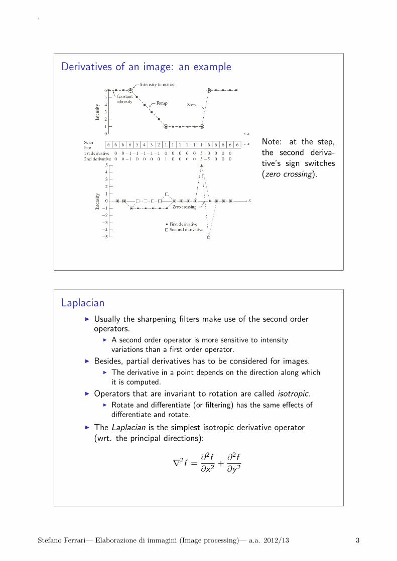
Derivatives of an image: an example

Note: at the step,the second deriva-tive’s sign switches(zero crossing).

Laplacian

I Usually the sharpening filters make use of the second orderoperators.

I A second order operator is more sensitive to intensityvariations than a first order operator.

I Besides, partial derivatives has to be considered for images.I The derivative in a point depends on the direction along which

it is computed.

I Operators that are invariant to rotation are called isotropic.I Rotate and differentiate (or filtering) has the same effects of

differentiate and rotate.

I The Laplacian is the simplest isotropic derivative operator(wrt. the principal directions):

∇2f =∂2f

∂x2+∂2f

∂y2

.


Laplacian filter

I In a digital image, the second derivatives wrt. x and y arecomputed as:

∂2f

∂x2= f (x + 1, y)− 2f (x , y) + f (x − 1, y)

∂2f

∂y2= f (x , y + 1)− 2f (x , y) + f (x , y − 1)

I Hence, the Laplacian results:

∇2f (x , y) = f (x + 1, y) + f (x − 1, y) + f (x , y + 1)

+f (x , y − 1)− 4f (x , y)

I Also the derivatives along to the diagonals can be considered:

∇2f (x , y) + f (x − 1, y − 1) + f (x + 1, y + 1)

+ f (x − 1, y + 1) + f (x + 1, y − 1)− 4f (x , y)

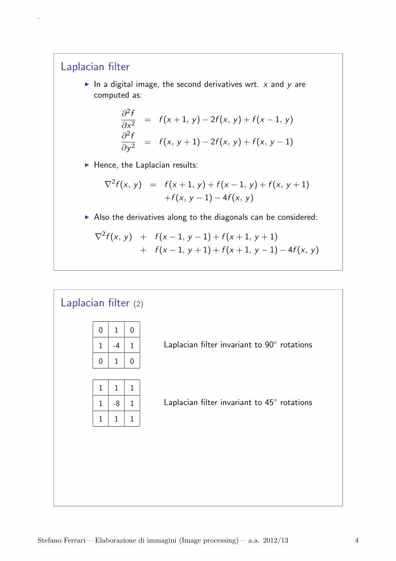
Laplacian filter (2)

0 1 0

1 -4 1

0 1 0

Laplacian filter invariant to 90◦ rotations

1 1 1

1 -8 1

1 1 1

Laplacian filter invariant to 45◦ rotations

.


Laplacian filter: example

I The Laplacian has often negative values.

I In order to be visualized, it must be properly scaled to therepresentation interval [0, . . . , L− 1].

(a) (b) (c)

(a) Original image, (b) its Laplacian, (c) its Laplacian scaled suchthat zero is displayed as the intermediate gray level.

Laplacian filter: example (2)

I The Laplacian is positive at the onset of a step and negativeat the end.

I Subtracting the Laplacian (or a fraction of it) from the image,the height of the step is increased.

(a) (b) (c)

(a) Original image, (b) Laplacian filtered, (c) Laplacian withdiagonals filtered.

.


Unsharp masking

I The technique known as unsharp masking is a method ofcommon use in graphics for making the images sharper.

I It consists of:

1. defocusing the original image;2. obtaining the mask as the difference between the original

image and its defocused copy;3. adding the mask to the original image.

I The process can be formalized as:

g = f + k · (f − f ∗ h)

where f is the original image, h is the smoothing filter and kis a constant for tuning the mask contribution.

I If k > 1, the process is called highboost filtering.

Unsharp masking (2)

original image

defocused image

unsharping mask

unsharped image

highboosted image

.


Gradient

I The gradient of a function is the vector formed by its partialderivatives.

I For a bidimensional function, f (x , y):

∇f ≡ grad(f ) ≡[gx

gy

]=

∂f

∂x∂f

∂y

I The gradient vector points toward the direction of maximumvariation.

I The gradient magnitude, M(x , y) is:

M(x , y) = mag(∇f ) =√

g2x + g2

y

I It is also called gradient image.I Often approximated as M(x , y) ≈ |gx |+ |gy |.

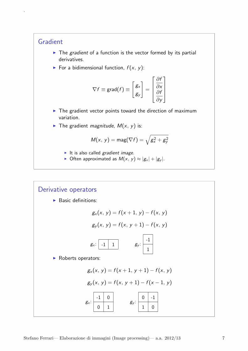
Derivative operators

I Basic definitions:

gx(x , y) = f (x + 1, y)− f (x , y)

gy (x , y) = f (x , y + 1)− f (x , y)

gx : -1 1 gy :-1

1

I Roberts operators:

gx(x , y) = f (x + 1, y + 1)− f (x , y)

gy (x , y) = f (x , y + 1)− f (x − 1, y)

gx :-1 0

0 1gy :

0 -1

1 0

.


Derivative operators (2)

I Sobel operators:

gx(x , y) = −f (x − 1, y − 1)− 2f (x − 1, y)

− f (x − 1, y + 1) + f (x + 1, y − 1)

+ 2f (x + 1, y) + f (x + 1, y + 1)

gy (x , y) = −f (x − 1, y − 1)− 2f (x , y − 1)

− f (x + 1, y − 1) + f (x − 1, y + 1)

+ 2f (x , y + 1) + f (x + 1, y + 1)

gx :

-1 -2 -1

0 0 0

1 2 1

gy :

-1 0 1

-2 0 2

-1 0 1

Example of gradient based application

I The Sobel filtering reduces the visibility of those regions inwhich the intensity changes slowly, allowing to highlight thedefects (and making defects detection easier for automaticprocessing).

.


Combined methods

I Often, a single technique is not sufficient for obtaining thedesired results.

I For example, the image (a) is affected by noise and has anarrow dynamic range.

(a) (b)

I Laplacian filtering (b)enhance the details,but also the noise.

I The gradient is lesssensitive to the noisethan the Laplacian(which is a secondorder operator).

Combined methods (2)

I The gradient, smoothed in order to avoid the noise, can beused for weighting the contribution of the Laplacian.

I The image (c), the Sobel filtering gradient smoothed using a5 × 5 averaging filter is reported.

(c) (d)

I This mask multipliedby the Laplacianresults in the image in(d).

I The intensity changesare preserved, whilethe noise has beenattenuated.

.


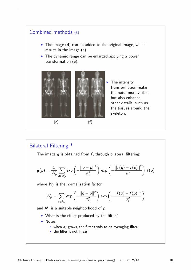
Combined methods (3)

I The image (d) can be added to the original image, whichresults in the image (e).

I The dynamic range can be enlarged applying a powertransformation (e).

(e) (f)

I The intensitytransformation makethe noise more visible,but also enhanceother details, such asthe tissues around theskeleton.

Bilateral Filtering *

The image g is obtained from f , through bilateral filtering:

g(p) =1

Wp

∑

q∈Np

exp

(−||q − p||2

σ2s

)exp

(−||f (q)− f (p)||2

σ2i

)f (q)

where Wp is the normalization factor:

Wp =∑

q∈Np

exp

(−||q − p||2

σ2s

)exp

(−||f (q)− f (p)||2

σ2i

)

and Np is a suitable neighborhood of p.

I What is the effect produced by the filter?I Notes:

I when σi grows, the filter tends to an averaging filter;I the filter is not linear.

.



(a) (b) (c)

(a) original image (100× 100, 256 gray levels)

(b) after filtering with Gaussian filter (7× 7, σs = 3)

(c) after filtering with bilateral filter (7× 7, σs = 3, σi = 50)


(a) (b) (c)

(a) Original image (107× 90, 256 gray levels)

(b) after filtering with Gaussian filter (7× 7, σs = 3)

(c) after filtering with bilateral filter (7× 7, σs = 3, σi = 30)

.


Homeworks and suggested readings

DIP, Sections 3.6, 3.7

I pp. 157–173

GIMPI Filters

I EnhanceI SharpenI Unsharp mask

I GenericI Convolution matrix

.
