SF2940: Probability theoryLecture 8: Multivariate Normal Distribution
Timo Koski
24.09.2015
Timo Koski Matematisk statistik 24.09.2015 1 / 1

Learning outcomes
Random vectors, mean vector, covariance matrix, rules oftransformation
Multivariate normal R.V., moment generating functions, characteristicfunction, rules of transformation
Density of a multivariate normal RV
Joint PDF of bivariate normal RVs
Conditional distributions in a multivariate normal distribution
Timo Koski Matematisk statistik 24.09.2015 2 / 1

PART 1: Mean vector, Covariance matrix, MGF,Characteristic function
Timo Koski Matematisk statistik 24.09.2015 3 / 1

Vector Notation: Random Vector
A random vector X is a column vector
X =
X1
X2...Xn
= (X1,X2, . . . ,Xn)T
Each Xi is a random variable.
Timo Koski Matematisk statistik 24.09.2015 4 / 1

Sample Value Random Vector
A column vector
x =
x1x2...xn
= (x1, x2, . . . , xn)T
We can think of xi is an outcome of Xi .
Timo Koski Matematisk statistik 24.09.2015 5 / 1

Joint CDF, Joint PDF
The joint CDF (=cumulative distribution function) of a continuousrandom vector X is
FX (x) = FX1,...,Xn(x1, . . . , xn) = P (X ≤ x) =
= P (X1 ≤ x1, . . . ,Xn ≤ xn)
Joint probability density function (PDF)
fX (x) =∂n
∂x1 . . . ∂xnFX1,...,Xn
(x1, . . . , xn)
Timo Koski Matematisk statistik 24.09.2015 6 / 1

Mean Vector
µX = E [X] =
E [X1]E [X2]
...E [Xn]
,
a column vector of means (=expectations) of X.
Timo Koski Matematisk statistik 24.09.2015 7 / 1

Matrix, Scalar Product
If XT is the transposed column vector (=a row vector), then
XXT
is a n× n matrix, and
XTX =n
∑i=1
X 2i
is a scalar product, a real valued R.V..
Timo Koski Matematisk statistik 24.09.2015 8 / 1
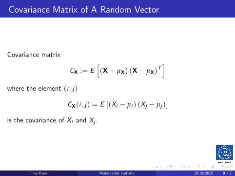
Covariance Matrix of A Random Vector
Covariance matrix
CX := E[
(X− µX) (X− µX)T]
where the element (i , j)
CX(i , j) = E [(Xi − µi ) (Xj − µj )]
is the covariance of Xi and Xj .
Timo Koski Matematisk statistik 24.09.2015 9 / 1
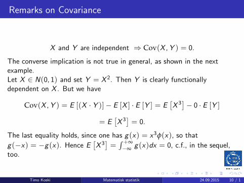
Remarks on Covariance
X and Y are independent ⇒ Cov(X ,Y ) = 0.
The converse implication is not true in general, as shown in the nextexample.Let X ∈ N(0, 1) and set Y = X 2. Then Y is clearly functionallydependent on X . But we have
Cov(X ,Y ) = E [(X · Y )]− E [X ] · E [Y ] = E[X 3]− 0 · E [Y ]
= E[X 3]= 0.
The last equality holds, since one has g(x) = x3φ(x), so that
g(−x) = −g(x). Hence E[X 3]=∫ +∞
−∞g(x)dx = 0, c.f., in the sequel,
too.
Timo Koski Matematisk statistik 24.09.2015 10 / 1

A Quadratic Form
xTCXx =n
∑i=1
n
∑j=1
xixjCX(i , j).
We see that
=n
∑i=1
n
∑j=1
xixjE [(Xi − µi ) (Xj − µj )]
= E
[n
∑i=1
n
∑j=1
xixj (Xi − µi ) (Xj − µj )
]
(∗)
Timo Koski Matematisk statistik 24.09.2015 11 / 1

Properties of a Covariance Matrix
Covariance matrix is nonnegative definite, i.e., for all x we have
xTCXx ≥ 0
HencedetCX ≥ 0.
The covariance matrix is symmetric
CX = CTX
Timo Koski Matematisk statistik 24.09.2015 12 / 1

Properties of a Covariance Matrix
The covariance matrix is symmetric
CX = CTX
sinceCX(i , j) = E [(Xi − µi ) (Xj − µj )]
= E [(Xj − µj ) (Xi − µi )] = CX(j , i)
Timo Koski Matematisk statistik 24.09.2015 13 / 1

Properties of a Covariance Matrix
A covariance matrix is positive definite,
xTCXx > 0
for all x 6= 0 iffdetCX > 0
(i.e. CX is invertible).
Timo Koski Matematisk statistik 24.09.2015 14 / 1

Properties of a Covariance Matrix
Proposition
xTCXx ≥ 0
Pf: By (∗) above
xTCXx = xTE[
(X− µX) (X− µX)T]
x
= E[
xT (X− µX) (X− µX)T x]
= E[
xTw ·wT x]
where we have set w = (X− µX). Then by linear algebra xTw = wTx= ∑
ni=1 wixi . Hence
E[
xTwwTx]
= E
(n
∑i=1
wixi
)2
≥ 0.
Timo Koski Matematisk statistik 24.09.2015 15 / 1

Properties of a Covariance Matrix
In terms of the entries ci ,j of a covariance matrix C = (ci ,j )n,n,i=1,j=1 there
are the following necessary properties.
1 ci ,j = cj ,i (symmetry).
2 ci ,i = Var (Xi ) = σ2i ≥ 0 (the elements in the main diagonal are the
variances, and thus all elements in the main diagonal arenonnegative).
3 c2i ,j ≤ ci ,i · cj ,j (Cauchy-Schwartz’ inequality).
Timo Koski Matematisk statistik 24.09.2015 16 / 1

Coefficient of Correlation
The Coefficient of Correlation ρ of X and Y is defined as
ρ := ρX ,Y :=Cov(X ,Y )
√
Var(X ) · Var(Y ),
where Cov(X ,Y ) = E [(X − µX ) (Y − µY )]. This is normalized
−1 ≤ ρX ,Y ≤ 1
For random variables X and Y ,
Cov(X ,Y ) = ρX ,Y = 0 does not always mean that X ,Y areindependent.
Timo Koski Matematisk statistik 24.09.2015 17 / 1

Special case: Covariance Matrix of A Bivariate Vector
X = (X1,X2)T .
CX =
(σ21 ρσ1σ2
ρσ1σ2 σ22
)
,
where ρ is the coefficient of correlation of X1 and X2, and σ21 = Var (X1),
σ22 = Var (X2). CX is invertible iff ρ2 6= 1, for proof we note that
detCX = σ21σ2
2
(1− ρ2
)
Timo Koski Matematisk statistik 24.09.2015 18 / 1
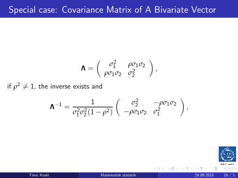
Special case: Covariance Matrix of A Bivariate Vector
Λ =
(σ21 ρσ1σ2
ρσ1σ2 σ22
)
,
if ρ2 6= 1, the inverse exists and
Λ−1 =1
σ21σ2
2 (1− ρ2)
(σ22 −ρσ1σ2
−ρσ1σ2 σ21
)
,
Timo Koski Matematisk statistik 24.09.2015 19 / 1

Y = BX+ b
Proposition
X is a random vector with mean vector µX and covariance matrix CX. B is
a m× n matrix. If Y = BX+ b, then
EY = BµX + b
CY = BCXBT
Pf: For simplicity of writing, take b = µ = 0. Then
CY = EYYT = EBX (BX)T =
= EBXXTBT = BE[
XXT]
BT = BCXBT
Timo Koski Matematisk statistik 24.09.2015 20 / 1

Moment Generating and Characteristic Functions
Definition
Moment generating function of X is defined as
ψX (t)def= Eet
TX = Eet1X1+t2X2+···+tnXn
Definition
Characteristic function of X is defined as
ϕX (t)def= Ee it
TX = Ee i (t1X1+t2X2+···+tnXn)
Special cases: take t1 = 1, t2 = t3 = . . . = tn = 0, thenϕX (t) = ϕX1 (t1).
Timo Koski Matematisk statistik 24.09.2015 21 / 1

PART 2: Def I of a multivariate normal distribution
We recall first some of the properties of univariate normal distribution
Timo Koski Matematisk statistik 24.09.2015 22 / 1

Normal (Gaussian) One-dimensional RVs
X is a normal random variable if
fX (x) =1
σ√2π
e− 1
2σ2(x−µ)2
where µ is real and σ > 0.
Notation: X ∈ N(µ, σ2)
Properties: E (X ) = µ, Var(X ) = σ2
Timo Koski Matematisk statistik 24.09.2015 23 / 1

Normal (Gaussian) One-dimensional RVs
−2 0 2 4 60
0.2
0.4
0.6
0.8
x
f X(x
)
−2 0 2 4 60
0.2
0.4
0.6
0.8
x
f X(x
) (a)
µ = 2, σ = 1/2 , (b) µ = 2, σ = 2
Timo Koski Matematisk statistik 24.09.2015 24 / 1

Central Moments Normal (Gaussian) One-dimensional RVs
X ∈ N(0, σ2). Then
E [X n] =
{
0 n is odd(2k)!2kk!
σ2k n = 2k , k = 0, 1, 2, . . ..
Timo Koski Matematisk statistik 24.09.2015 25 / 1

Linear Transformation
X ∈ N(µX , σ2) ⇒ Y = aX + b is N(aµX + b, a2σ2)
Thus Z = X−µX
σX∈ N(0, 1) and
P(X ≤ x) = P
(X − µX
σX≤ x − µX
σX
)
or
FX (x) = P
(
Z ≤ x − µX
σX
)
= Φ
(x − µX
σX
)
Timo Koski Matematisk statistik 24.09.2015 26 / 1

Normal (Gaussian) One-dimensional RVs
X ∈ N(µ, σ2) then the moment generating function is
ψX (t) = E[
etX]
= etµ+ 12 t
2σ2,
and the characteristic function is
ϕX (t) = E[
e itX]
= e itµ− 12 t
2σ2
as found in previous Lectures.
Timo Koski Matematisk statistik 24.09.2015 27 / 1

Multivariate Normal Def. I
Definition
An n× 1 random vector X has a normal distribution iff for every
n× 1-vector a the one-dimensional random vector aTX has a normal
distribution.
We write X ∈ N (µ,Λ), when µ is the mean vector and Λ is thecovariance matrix.
Timo Koski Matematisk statistik 24.09.2015 28 / 1

Consequences of Def. I (1)
An n× 1 vector X ∈ N (µ,Λ) iff the one-dimensional random vector aTXhas a normal distribution for every n-vector a .
Now we know that (take B = aT in the preceding)
EaTX = aTµ,Var[
aTX]
= aTΛa
Timo Koski Matematisk statistik 24.09.2015 29 / 1

Consequences of Def. I (2)
Hence, if Y = aTX, then Y ∈ N(aTµ, aTΛa
)and the moment
generating function of Y is
ψY (t) = E[
etY]
= etaT µ+ 1
2 t2aTΛa.
ThereforeψX (a) = Eea
TX = ψY (1) = eaT µ+ 1
2aTΛa.
Timo Koski Matematisk statistik 24.09.2015 30 / 1

Consequences of Def. I (3)
Hence we have shown that if X ∈ N (µ,Λ), then
ψX (t) = EetTX = et
T µ+ 12 t
TΛt.
is the moment generating function of X.
Timo Koski Matematisk statistik 24.09.2015 31 / 1

Consequences of Def. I (4)
In the same way we can find that
ϕX (t) = Ee itTX = e it
T µ− 12 t
TΛt.
is the characteristic function of X ∈ N (µ,Λ).
Timo Koski Matematisk statistik 24.09.2015 32 / 1

Consequences of Def. I (5)
Let Λ be a diagonal covariance matrix with λ2i s on the main diagonal, i.e.,
Λ =
λ21 0 0 . . . 00 λ2
2 0 . . . 00 0 λ2
3 . . . 0
0. . .
... . . . 00 0 0 . . . λ2
n
,
Proposition
If X ∈ N (µ,Λ), then X1,X2, . . . ,Xn are independent normal variables.
Timo Koski Matematisk statistik 24.09.2015 33 / 1

Consequences of Def. I (6)
Pf: Λ is diagonal, the quadratic form becomes a single sum of squares.
ϕX (t) = e itT µ− 1
2 tTΛt =
= e i ∑ni=1 µi ti− 1
2 ∑ni=1 λ2
i t2i
= e iµ1t1− 12 λ2
1t21 e iµ2t2− 1
2 λ22t
22 · · · e iµntn− 1
2 λ2nt
2n
is the product of the characteristic functions of Xi ∈ N(µi ,λ2
i
), which are
thus seen to be independent N(µi ,λ2
i
).
Timo Koski Matematisk statistik 24.09.2015 34 / 1

Kac’s theorem: Thm 8.1.3. in LN
Theorem
X = (X1,X2, · · · ,Xn)T . The components X1,X2, · · · ,Xn areindependent if and only if
φX (s) = E[
e is′X]
=n
∏i=1
φXi(si ),
where φXi(si ) is the characteristic function for Xi .
Timo Koski Matematisk statistik 24.09.2015 35 / 1
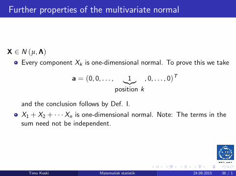
Further properties of the multivariate normal
X ∈ N (µ,Λ)
Every component Xk is one-dimensional normal. To prove this we take
a = (0, 0, . . . , 1︸︷︷︸
position k
, 0, . . . , 0)T
and the conclusion follows by Def. I.
X1 + X2 + · · ·Xn is one-dimensional normal. Note: The terms in thesum need not be independent.
Timo Koski Matematisk statistik 24.09.2015 36 / 1

Properties of multivariate normal
X ∈ N (µ,Λ)
Every marginal distribution of k variables ( 1 ≤ k < n is normal. Toprove this we consider any k variables Xi1 ,Xi2 . . . Xik and then take asuch that aj = 0 for j 6= i1, . . . ik and then apply Def. I.
Timo Koski Matematisk statistik 24.09.2015 37 / 1

Properties of multivariate normal
Proposition
X ∈ N (µ,Λ) and Y = BX+ b. Then
Y ∈ N(
Bµ + b,BΛBT)
.
Pf:ψY (s) = E
[
esTY]
= E[
esT (b+BX)
]
=
= esT bE
[
esTBX
]
= esT bE
[
e(BT s)
TX
]
E
[
e(BT s)
TX
]
= ψX
(
BT s)
.
Timo Koski Matematisk statistik 24.09.2015 38 / 1
Properties of multivariate normal
X ∈ N (µ,Λ)
ψX
(
BT s)
= e(BT s)
Tµ+ 1
2 (BT s)TΛ(BT s).
(
BT s)T
µ = sTBµ,
(
BT s)T
Λ(
BT s)
= sTBΛBTs,
e(BT s)
Tµ+ 1
2(BT s)TΛ(BT s) = es
TBµ+ 12 s
TBΛBT s
Timo Koski Matematisk statistik 24.09.2015 39 / 1

Properties of multivariate normal
ψX
(
BT s)
= esTBµ+ 1
2 sTBΛBT s.
ψY (s) = esTbψX
(
BT s)
= esTbes
TBµ+ 12 s
TBΛBT s
ψY (s) = esT (b+Bµ)+ 1
2 sTBΛBT s,
which proves the claim as asserted.
Timo Koski Matematisk statistik 24.09.2015 40 / 1

PART 3: Multivariate normal, Def. II: characteristic
function, DEF III: density
Timo Koski Matematisk statistik 24.09.2015 41 / 1

Multivariate normal, Def. II: char. fnctn
Definition
A random vector X with mean vector µ and a covariance matrix Λ is
N (µ,Λ) if its characteristic function is
ϕX (t) = Ee itTX = e it
T µ− 12 t
TΛt.
Timo Koski Matematisk statistik 24.09.2015 42 / 1

Multivariate normal, Def. II implies Def. I
We need to show that the one-dimensional random vector Y = aTX has anormal distribution.
ϕY (t) = E[
e itY]
= E[
e it ∑ni=1 ai ·Xi
]
=
= E[
e itaTX]
= ϕX (ta) =
= e itaT µ− 1
2 t2aTΛa
and this is the characteristic function of N(aTµ, aTΛa
).
Timo Koski Matematisk statistik 24.09.2015 43 / 1

Multivariate normal, Def. III: joint PDF
Definition
A random vector X with mean vector µ and an invertible covariance
matrix Λ is N (µ,Λ), if the density is
fX (x) =1
(2π)n/2√
det(Λ)e−
12 (x−µ)TΛ−1(x−µ)
Timo Koski Matematisk statistik 24.09.2015 44 / 1

Multivariate normal
It can be checked by a computation that
e itT µ− 1
2 tTΛt =
∫
Rne it
T x 1
(2π)n/2√
det(Λ)e−
12 (x−µ)TΛ−1(x−µ)dx
(complete the square) Hence Def. III implies the property in Def. II. Thethree definitions are equivalent, in the case inverse of the covariancematrix exists.
Timo Koski Matematisk statistik 24.09.2015 45 / 1

PART 4: Bivariate normal with density
Timo Koski Matematisk statistik 24.09.2015 46 / 1

Multivariate Normal: the bivariate case
As soon as ρ2 6= 1, the matrix
Λ =
(σ21 ρσ1σ2
ρσ1σ2 σ22
)
,
is invertible, and the inverse is
Λ−1 =1
σ21σ2
2 (1− ρ2)
(σ22 −ρσ1σ2
−ρσ1σ2 σ21
)
,
Timo Koski Matematisk statistik 24.09.2015 47 / 1

Multivariate Normal: the bivariate case
ρ2 6= 1, and X = (X1,X2)T , then
fX (x) =1
2π√detΛ
e−12 (x−µX)
TΛ−1(x−µX)
=1
2πσ1σ2√
1− ρ2e−
12Q(x1,x2)
Timo Koski Matematisk statistik 24.09.2015 48 / 1

Multivariate Normal: the bivariate case
whereQ(x1, x2) =
1
(1− ρ2)·[(
x1 − µ1
σ1
)2
− 2ρ(x1 − µ1)(x2 − µ2)
σ1σ2+
(x2 − µ2
σ2
)2]
For this, invert the matrix Λ and expand the quadratic form !
Timo Koski Matematisk statistik 24.09.2015 49 / 1
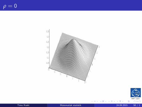
ρ = 0
0
0.35
0.3
0.25
0.2
0.15
0.1
0.05
0
0
32
10
-1-2
-3
0
3
2
1
0
-1
-2
-3
Timo Koski Matematisk statistik 24.09.2015 50 / 1

ρ = 0.9
0
0.35
0.3
0.25
0.2
0.15
0.1
0.05
0
0
32
10
-1-2
-3
0
3
2
1
0
-1
-2
-3
Timo Koski Matematisk statistik 24.09.2015 51 / 1
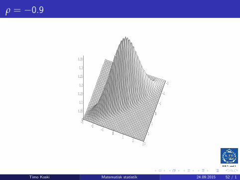
ρ = −0.9
0
0.35
0.3
0.25
0.2
0.15
0.1
0.05
0
0
32
10
-1-2
-3
0
3
2
1
0
-1
-2
-3
Timo Koski Matematisk statistik 24.09.2015 52 / 1

Conditional densities for the bivariate normal
Complete the square of the exponent to write
fX ,Y (x , y ) = fX (x)fY |X (y )
where
fX (x) =1
σ1√2π
e− 1
2σ21(x−µ1)2
fY |X (y ) =1
σ̃2√2π
e− 1
2σ̃22(y−µ̃2(x))2
µ̃2(x) = µ2 + ρσ2σ1
(x − µ1), σ̃2 = σ2
√
1− ρ2
Timo Koski Matematisk statistik 24.09.2015 53 / 1
Bivariate normal properties
E (X ) = µ1
Given X = x , Y is Gaussian
Conditional mean of Y given X = x :
µ̃2(x) = µ2 + ρσ2σ1
(x − µ1) = E (Y |X = x)
Conditional variance of Y given X = x :
Var(Y |X = x) = σ22
(1− ρ2
)
Timo Koski Matematisk statistik 24.09.2015 54 / 1

Bivariate normal properties
Conditional mean of Y given X = x :
µ̃2(x) = µ2 + ρσ2σ1
(x − µ1) = E (Y |X = x)
Conditional variance of Y given X = x :
Var(Y |X = x) = σ22
(1− ρ2
)
Check Section 3.7.3. and Exercise 3.8.4.6. By this is seen that theconditional mean of Y given X variable in a bivariate normaldistribution is also the best LINEAR predictor of Y based on X , andthe conditional variance is the variance of the estimation error.
Timo Koski Matematisk statistik 24.09.2015 55 / 1

Marginal PDFs
Timo Koski Matematisk statistik 24.09.2015 56 / 1

Proof of conditional pdf
Consider
fX ,Y (x , y )
fX (x)=
σ1√2π
2πσ1σ2√
1− ρ2e− 1
2Q(x ,y )+ 1
2σ21(x−µ1)2
Timo Koski Matematisk statistik 24.09.2015 57 / 1

Proof of conditional pdf
−1
2Q(x , y ) +
1
2σ21
(x − µ1)2
= −1
2H(x , y ),
Timo Koski Matematisk statistik 24.09.2015 58 / 1

Proof of conditional pdfs
H(x , y ) =
1
(1− ρ2)·[(
x − µ1
σ1
)2
− 2ρ(x − µ1)(y − µ2)
σ1σ2+
(y − µ2
σ2
)2]
−(x − µ1
σ1
)2
Timo Koski Matematisk statistik 24.09.2015 59 / 1

Proof of conditional pdf
H(x , y ) =
ρ2
(1− ρ2)
(x − µ1)2
σ21
− 2ρ(x − µ1)(y − µ2)
σ1σ2(1− ρ2)+
(y − µ2)2
σ22 (1− ρ2)
Timo Koski Matematisk statistik 24.09.2015 60 / 1

Proof of conditional pdf
H(x , y ) =
(
y − µ2 − ρ σ2σ1(x − µ1)
)2
σ22 (1− ρ2)
Timo Koski Matematisk statistik 24.09.2015 61 / 1

Conditional pdf
fX ,Y (x , y )
fX (x)=
1√
1− ρ2σ2√2π
e
− 12
(y−µ2−ρσ2σ1
(x−µ1))2
σ22 (1−ρ2)
This establishes the bivariate normal properties claimed above.
Timo Koski Matematisk statistik 24.09.2015 62 / 1

Bivariate normal properties : ρ
Proposition
(X ,Y ) bivariate normal ⇒ ρ = ρX ,Y
Proof:
E [(X − µ1)(Y − µ2)]
= E (E ([(X − µ1)(Y − µ2)] |X ))
= E ((X − µ1)E [Y − µ2] |X ))
Timo Koski Matematisk statistik 24.09.2015 63 / 1
Bivariate normal properties : ρ
= E ((X − µ1)E [(Y − µ2)] |X ))
= E (X − µ1) [E (Y |X )− µ2]
= E ((X − µ1)
[
µ2 + ρσ2σ1
(X − µ1)− µ2
]
= ρσ2σ1
E (X − µ1)((X − µ1))
Timo Koski Matematisk statistik 24.09.2015 64 / 1

Bivariate normal properties : ρ
= ρσ2σ1
E (X − µ1)(X − µ1)
= ρσ2σ1
E (X − µ1)2
= ρσ2σ1
σ21
= ρσ2σ1
Timo Koski Matematisk statistik 24.09.2015 65 / 1

Bivariate normal properties : ρ
In other words we have checked that
ρ =E [(X − µ1)(Y − µ2)]
σ2σ1
ρ = 0 ⇔ bivariate normal X ,Y are independent.
Timo Koski Matematisk statistik 24.09.2015 66 / 1

PART 5: Generating a multivariate normal variable
Timo Koski Matematisk statistik 24.09.2015 67 / 1

Standard Normal Vector: definition
Z ∈ N (0, I) is a standard normal vector.I is the n× n identity matrix.
fZ (z) =1
(2π)n/2√
det(I)e−
12 (z−0)T I−1(z−0)
=1
(2π)n/2e−
12 z
T z
Timo Koski Matematisk statistik 24.09.2015 68 / 1

Distribution of X = AZ+ b
X = AZ+ b, Z is standard Gaussian, then
X = N(
b,AAT)
(follows by a rule in the preceding)
Timo Koski Matematisk statistik 24.09.2015 69 / 1

Multivariate Normal: the bivariate case
If
Λ =
(σ21 ρσ1σ2
ρσ1σ2 σ22
)
,
then Λ = AAT , where
A =
(σ1 0
ρσ2 σ2√
1− ρ2
)
,
Timo Koski Matematisk statistik 24.09.2015 70 / 1

Standard Normal Vector
X ∈ N (µX,Λ), and A is such that
Λ = AAT
(An invertible matrix A with this property exists always, if Λ is positivedefinite (we need the symmetry of Λ, too.) Then
Z = A−1 (X− µX)
is a standard Gaussian vector.Proof: We give the first idea of his proof, a rule of transformation.
Timo Koski Matematisk statistik 24.09.2015 71 / 1
Rule of transformation
If X has density fX (x), Y = AX+ b,A is invertible, then
fY (y) =1
| detA | fX(A−1 (y− b)
)
Note that if Λ = AAT , then
detΛ = detA · detAT = detA · detA = detA2,
so that | detA| =√detΛ.
Timo Koski Matematisk statistik 24.09.2015 72 / 1

Diagonalizable Matrices
An n× n matrix A is orthogonally diagonalizable, if there is anorthogonal matrix P (i.e., PTP =PPT = I) such that
PTAP = Λ,
where Λ is a diagonal matrix.
Timo Koski Matematisk statistik 24.09.2015 73 / 1

Diagonalizable Matrices
Theorem
If A is an n× n matrix, then the following are equivalent:
(i) A is orthogonally diagonalizable.
(ii) A has an orthonormal set of eigenvectors.
(iii) A is symmetric.
Since covariance matrices are symmetric, we have by the theorem abovethat all covariance matrices are orthogonally diagonalizable.
Timo Koski Matematisk statistik 24.09.2015 74 / 1
Diagonalizable Matrices
Theorem
If A is a symmetric matrix, then
(i) Eigenvalues of A are all real numbers.
(ii) Eigenvectors from different eigenspaces are orthogonal.
That is, all eigenvalues of a covariance matrix are real.
Timo Koski Matematisk statistik 24.09.2015 75 / 1
Diagonalizable Matrices
Hence we have for any covariance matrix the spectral decomposition
C =n
∑i=1
λieieTi , (1)
where Cei = λiei . Since C is nonnegative definite, and its eigenvectors areorthonormal,
0 ≤ eTi Cei = λieTi ei = λi ,
and thus the eigenvalues of a covariance matrix are nonnegative.
Timo Koski Matematisk statistik 24.09.2015 76 / 1

Diagonalizable Matrices
Let now P be an orthogonal matrix such that
P′CXP = Λ,
and X ∈ N (0,CX), i.e., CX is a covariance matrix and Λ is diagonal (withthe eigenvalues of CX on the main diagonal). Then if Y = PTX, we havethat
Y ∈ N (0,Λ) .
In other words, Y is a Gaussian vector and has independent components.This method of producing independent Gaussians has several importantapplications. One of these is the principal component analysis.
Timo Koski Matematisk statistik 24.09.2015 77 / 1

Timo Koski Matematisk statistik 24.09.2015 78 / 1
Recommended