Sensitivity of snow density and specific surface areameasured by microtomography to different imageprocessing algorithmsPascal Hagenmuller1,2, Margret Matzl3, Guillaume Chambon2, andMartin Schneebeli3
1Météo-France - CNRS, CNRM-GAME, UMR 3589, CEN, 38400 Saint Martin d’Hères, France2Irstea, UR ETGR Erosion torrentielle, neige et avalanches, 38402 Saint Martin d’Hères, France3WSL Institute for Snow and Avalanche Research SLF, Fluelastrasse 11, 7260 Davos Dorf,Switzerland
Correspondence to: Pascal Hagenmuller ([email protected])
Abstract. Microtomography can measure the X-ray attenuation coefficient in a 3D volume of snow
with a spatial resolution of a few microns. In order to extract quantitative characteristics of the
microstructure, such as the specific surface area (SSA), from these data, the grayscale image first
needs to be segmented into a binary image of ice and air. Different numerical algorithms can then
be used to compute the surface area of the binary image. In this paper, we report on the effect of5
commonly used segmentation and surface area computation techniques on the evaluation of density
and specific surface area. The evaluation is based on a set of 38 X-ray tomographies of different
snow samples without impregnation, scanned with an effective voxel size of 10 and 18 µm. We
found that different surface area computation methods can induce relative variations up to 5% in the
density and SSA values. Regarding segmentation, similar results were obtained with sequential and10
energy-based approaches provided the associated parameters are correctly chosen. The voxel size
also appears to affect the values of density and SSA, but because images with the higher resolution
also show the higher noise level, it was not possible to draw a definitive conclusion on this effect
of resolution. Finally, practical recommendations concerning the processing of X-ray tomographic
images of snow are provided.15
1 Introduction
The specific surface area (SSA) of snow is defined as the area S of the ice-air interface per unit
mass M , i.e. SSA= S/M expressed in m2 kg−1. This quantity is essential for the modelling of the
physical and chemical properties of snow because it is an indicator of potential exchanges with the
1
The Cryosphere Discuss., doi:10.5194/tc-2015-217, 2016Manuscript under review for journal The CryospherePublished: 25 January 2016c© Author(s) 2016. CC-BY 3.0 License.

surrounding environment. For instance, SSA can be used to predict snow electromagnetic character-20
istics such as light scattering and absorption (albedo in the near infrared) (e.g. Warren, 1982; Flanner
and Zender, 2006) or microwave radiation (e.g. Brucker et al., 2011), and snow metamorphism (e.g.
Flin et al., 2004; Domine et al., 2007). Precise knowledge of this quantity is required in numer-
ous applications such as cold regions hydrology, predicting the role of snow in the regional/global
climate system, optical and microwave remote sensing, snow chemistry, etc.25
In the last decade, numerous field and laboratory instruments were developed by different research
groups to measure snow grain size. One possible definition of this grain size is the equivalent spher-
ical radius req , computed from the SSA as req = 3/(ρice×SSA) with ρice the density of ice. This
definition is actually equivalent to the optical radius, i.e. the radius of a collection of spheres with the
same infrared albedo as that of the snow microstructure (Warren, 1982). In contrast, the definition30
of grain size used in traditional snow classification as the mean of the longest extension of disag-
gregated particles (Fierz et al., 2009) is correlated to SSA only for a few snow classes. The crystal
size as stereologically measured by Riche et al. (2012) is equivalent to req only for monocrystalline
snow grains. Because of the co-existence of these inconsistent grain size definitions and of different
associated measurement methods (optical, gas adsorption, tomography, stereology), an intercompar-35
ison of different grain size measurement methods was organised by the International Association
of Cryospheric Sciences (IACS) working group "From quantitative stratigraphy to microstructure-
based modelling of snow". One of the main objectives of this intercomparison was to determine the
accuracy, comparability and quality of existing measurement methods.
In the context of this workshop, the present study focuses on the measurement of density and SSA40
derived from microtomographic data (Cnudde and Boone, 2013). Microtomography measures the
X-ray attenuation coefficient in a three-dimensional (3D) volume with high spatial resolutions of a
few to a few tens of microns. To extract the microstructure from the reconstructed 3D image, this
image has to be filtered to reduce noise and subsequently analysed to identify the phase relevant
for the investigation, in our case ice. This step, called binary segmentation, affects the subsequent45
microstructure characterisation, especially when the image resolution is close to the typical size of
microstructural details. Different algorithms then exist to calculate density and SSA from this im-
ages. Here we investigate the effects of binary segmentation and surface area calculation methods
on density and SSA estimates, in order to provide guidelines for the use of snow sample microtomo-
graphic data.50
Comparative studies of processing techniques for images obtained via X-ray microtomography
have already listed the performance of several segmentation methods with respect to different qual-
ity indicators (e.g. Kaestner et al., 2008; Iassonov et al., 2009; Schlüter and Sheppard, 2014). These
studies emphasised the importance of using local image information such as spatial correlation to
perform suitable segmentations and highlighted the superior performance of Bayesian Markov ran-55
dom field segmentation (Berthod et al., 1996), which consists in finding the segmentation with min-
2
The Cryosphere Discuss., doi:10.5194/tc-2015-217, 2016Manuscript under review for journal The CryospherePublished: 25 January 2016c© Author(s) 2016. CC-BY 3.0 License.

imum boundary surface and which at the same time respects the gray value data in the best possible
way. However, none of the mentioned studies were interested in snow. This material exhibits specific
features such as a natural tendency, induced by metamorphism, to minimise its surface energy (e.g.
Flin et al., 2003; Vetter et al., 2010). Moreover, these former studies tended to focus on properties60
linked to volumetric material contents, while less attention was paid to the surface area of the seg-
mented object. Hagenmuller et al. (2013) applied an energy-based segmentation method on images
of impregnated snow samples, which is a three-phase material (impregnation product, ice and resid-
ual air bubbles). This method is based on the same principles as the Bayesian Markov random field
segmentation but the optimisation process is performed differently. It takes explicitly advantage of65
the knowledge that the surface energy of snow tends to be minimal, and was shown to be accurate
in comparison to a segmentation method based on global thresholding. However the set of snow
microtomographic images used by Hagenmuller et al. (2013) was limited to impregnated samples
and to a few different snow types. Moreover, no independent SSA measurements were available to
provide a reference or at least a comparison. Here, the flexible energy-based segmentation method70
was adapted to two-phase images (air-ice) and applied to 38 images on which SSA measurements
were conducted with independent instruments. Note that comparisons with these independent SSA
measurements are beyond the scope of this paper and will be reported in a synthesis paper of the
working group to be published in the present special issue of The Cryosphere.
First, the sampling and X-ray measurement procedures to obtain grayscale images are described.75
Attention is paid to the fact that the parameters used for binary segmentation also depend on the
scanned sample and not only on the X-ray source setup. Second, two different approaches of binary
segmentation are presented. The first one, commonly used in the snow science community, con-
sists of a sequence of filters: Gaussian smoothing, global thresholding and morphological filtering.
The second one is based on the minimisation of a segmentation energy. Third, different methods80
to compute surface area from binary images are presented. Finally, the different methods of binary
segmentation and area computation are applied to the microtomographic images and the results are
compared to provide an estimation of the scatter in density and SSA measurements due to numerical
processing of the grayscale image and area calculation.
2 Material and methods85
2.1 Data set
Snow sampling, preparation and scanning were conducted at SLF, Davos, Switzerland, during the
Snow Grain Size Workshop in March 2014.
3
The Cryosphere Discuss., doi:10.5194/tc-2015-217, 2016Manuscript under review for journal The CryospherePublished: 25 January 2016c© Author(s) 2016. CC-BY 3.0 License.

A5 (FC/DF)
N1 (RG)
M2-2 (DH/FC)
F2-2 (FCxr)E4 (RG/DF)
C4 (RG)B5 (FC/RG) D5 (FC/RG)
D5-2 (FC/RG) G2 (RG/FC)
H2 (FC/FCxr) M1-1 (DH/FC) M1-3 (DHch/FC)
3 mm
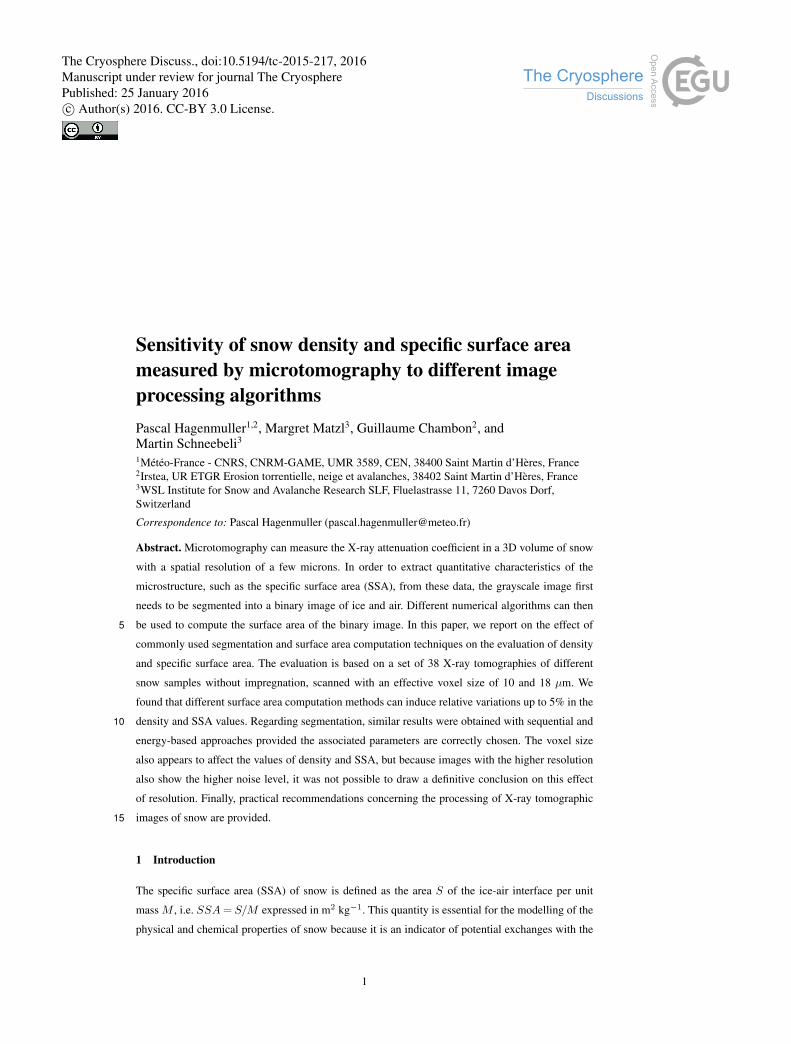
Figure 1. The different snow types and microstructural patterns used in this study. The 3D images shown have
a side-length of 3 mm and correspond to a subset of the images analysed in the present study. The grain shape
is also indicated in brackets below the images, according to the international snow classification (Fierz et al.,
2009).
2.1.1 Sampling
Thirteen snow blocks of apparently homogeneous snow were collected in the field or prepared in90
a cold laboratory. These blocks span different snow types (decomposing and fragmented snow,
rounded grains, faceted crystals and depth hoar, Fig. 1). Smaller specimens were taken out of these
blocks to conduct grain size measurements with different instruments. Two snow cylinders of ra-
dius 35 mm and height of 60 mm and one snow cylinder of radius 20 mm and 60 mm height were
extruded from each block to perform microtomographic measurements.95
4
The Cryosphere Discuss., doi:10.5194/tc-2015-217, 2016Manuscript under review for journal The CryospherePublished: 25 January 2016c© Author(s) 2016. CC-BY 3.0 License.
1 mm
Number of voxels
Intensity (arbitrary units)Ice
Air
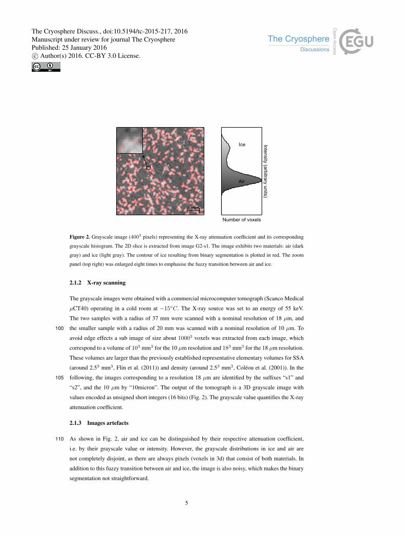
Figure 2. Grayscale image (4002 pixels) representing the X-ray attenuation coefficient and its corresponding
grayscale histogram. The 2D slice is extracted from image G2-s1. The image exhibits two materials: air (dark
gray) and ice (light gray). The contour of ice resulting from binary segmentation is plotted in red. The zoom
panel (top right) was enlarged eight times to emphasise the fuzzy transition between air and ice.
2.1.2 X-ray scanning
The grayscale images were obtained with a commercial microcomputer tomograph (Scanco Medical
µCT40) operating in a cold room at −15◦C. The X-ray source was set to an energy of 55 keV.
The two samples with a radius of 37 mm were scanned with a nominal resolution of 18 µm, and
the smaller sample with a radius of 20 mm was scanned with a nominal resolution of 10 µm. To100
avoid edge effects a sub image of size about 10003 voxels was extracted from each image, which
correspond to a volume of 103 mm3 for the 10 µm resolution and 183 mm3 for the 18 µm resolution.
These volumes are larger than the previously established representative elementary volumes for SSA
(around 2.53 mm3, Flin et al. (2011)) and density (around 2.53 mm3, Coléou et al. (2001)). In the
following, the images corresponding to a resolution 18 µm are identified by the suffixes “s1” and105
“s2”, and the 10 µm by “10micron”. The output of the tomograph is a 3D grayscale image with
values encoded as unsigned short integers (16 bits) (Fig. 2). The grayscale value quantifies the X-ray
attenuation coefficient.
2.1.3 Images artefacts
As shown in Fig. 2, air and ice can be distinguished by their respective attenuation coefficient,110
i.e. by their grayscale value or intensity. However, the grayscale distributions in ice and air are
not completely disjoint, as there are always pixels (voxels in 3d) that consist of both materials. In
addition to this fuzzy transition between air and ice, the image is also noisy, which makes the binary
segmentation not straightforward.
5
The Cryosphere Discuss., doi:10.5194/tc-2015-217, 2016Manuscript under review for journal The CryospherePublished: 25 January 2016c© Author(s) 2016. CC-BY 3.0 License.

30000 35000 40000 45000 50000Intensity (arbitrary units)
0
5
10
15
20
25
30
35
40
Occ
uren
ce ra
tio (1
0−5)
Sampless1 and s210micron
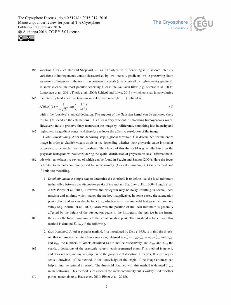
Figure 3. Grayscale distributions for all images. The solid lines and dashed lines respectively represent the dis-
tributions for the images scanned with the resolution 10 µm and 18 µm. The grayscale distribution is computed
on 1000 bins of homogeneous size in the intensity range [30000,50000] (arbitrary units).
Figure 3 shows the grayscale distributions obtained on all scanned images. The exact position of115
the attenuation peaks and the scatter around the peaks depend both on resolution and snow sample.
Slight differences are also observed between the grayscale distribution of the two images coming
from the same snow block and scanned with the same resolution. This may be due slight variations
in the temperature of the X-ray source during successive scans. Hence, it is doubtful whether binary
segmentation parameters “optimised” for one image can be used to segment other images even of120
the same sample and with the same resolution. It appears necessary to determine the segmentation
parameters on each image independently.
2.2 Segmentation methods
In this section, two binary segmentation methods are presented: (1) the common method based on
global thresholding combined with denoising and morphological filtering, hereafter referred to as125
sequential filtering, and (2) a method based on the minimisation of a segmentation energy, referred
to as energy-based segmentation.
2.2.1 Sequential filtering
Sequential filtering is commonly used to segment grayscale microtomographic images of snow be-
cause it is simple, fast, and is implemented in packages of several different programming languages.130
It consists of a sequence of denoising, global thresholding and post-processing, the input of each
step coming from the output of the previous step.
Denoising with a Gaussian filter. Numerous filters exist to remove noise from images, the most
common being the Gaussian filter, the median filter, the anisotropic diffusion filter and the total
6
The Cryosphere Discuss., doi:10.5194/tc-2015-217, 2016Manuscript under review for journal The CryospherePublished: 25 January 2016c© Author(s) 2016. CC-BY 3.0 License.
variation filter (Schlüter and Sheppard, 2014). The objective of denoising is to smooth intensity135
variations in homogeneous zones (characterised by low-intensity gradients) while preserving sharp
variations of intensity in the transition between materials (characterised by high-intensity gradient).
In snow science, the most popular denoising filter is the Gaussian filter (e.g. Kerbrat et al., 2008;
Lomonaco et al., 2011; Theile et al., 2009; Schleef and Löwe, 2013), which consists in convoluting
the intensity field I with a Gaussian kernel of zero mean N (0,σ) defined as:140
N (0,σ)(I) =1
σ√
2πexp
(− I2
2σ2
)(1)
with σ the (positive) standard deviation. The support of the Gaussian kernel can be truncated (here
to b4σc) to speed up the calculations. This filter is very efficient in smoothing homogeneous zones.
However it fails to preserve sharp features in the image by indifferently smoothing low-intensity and
high-intensity gradient zones, and therefore reduces the effective resolution of the image.145
Global thresholding. After the denoising step, a global threshold T is determined for the entire
image in order to classify voxels as air or ice depending whether their grayscale value is smaller
or greater, respectively, than the threshold. The choice of this threshold is generally based on the
grayscale histogram without considering the spatial distribution of grayscale values. Different meth-
ods exist, an exhaustive review of which can be found in Sezgin and Sankur (2004). Here the focus150
is limited to methods commonly used for snow, namely: (1) local minimum, (2) Otsu’s method, and
(3) mixture modelling.
1. Local minimum: A simple way to determine the threshold is to define it as the local minimum
in the valley between the attenuation peaks of ice and air (Fig. 3) (e.g. Flin, 2004; Heggli et al.,
2009; Pinzer et al., 2012). However, the histogram may be noisy, resulting in several local155
maxima and minima, which makes the method inapplicable. In some cases, the attenuation
peaks of ice and air can also be too close, which results in a unimodal histogram without any
valley (e.g. Kerbrat et al., 2008). Moreover, the position of the local minimum is generally
affected by the height of the attenuation peaks in the histogram: the less ice in the image,
the closer the local minimum is to the ice attenuation peak. The threshold obtained with this160
method is denoted Tvalley in the following.
2. Otsu’s method: Another popular method, first introduced by Otsu (1975), is to find the thresh-
old that minimises the intra-class variance σw defined as σ2w = nairσ
2air +niceσ
2ice, with nair
and nice the numbers of voxels classified as air and ice respectively, and σair and σice the
standard deviations of the grayscale value in each segmented class. This method is generic165
and does not require any assumption on the grayscale distribution. However, this also repre-
sents a drawback of the method, in that knowledge of the origin of the image artefacts can
help to find the optimal threshold. The threshold obtained with this method is denoted Totsu
in the following. This method is less used in the snow community but is widely used for other
porous materials (e.g. Haussener, 2010; Ebner et al., 2015).170
7
The Cryosphere Discuss., doi:10.5194/tc-2015-217, 2016Manuscript under review for journal The CryospherePublished: 25 January 2016c© Author(s) 2016. CC-BY 3.0 License.
3. Mixture modelling: The classification error induced by the thresholding can be also minimised
by assuming that each class is Gaussian-distributed. From there, different methods can be
considered to decompose the grayscale histogram in a sum of Gaussian distributions:
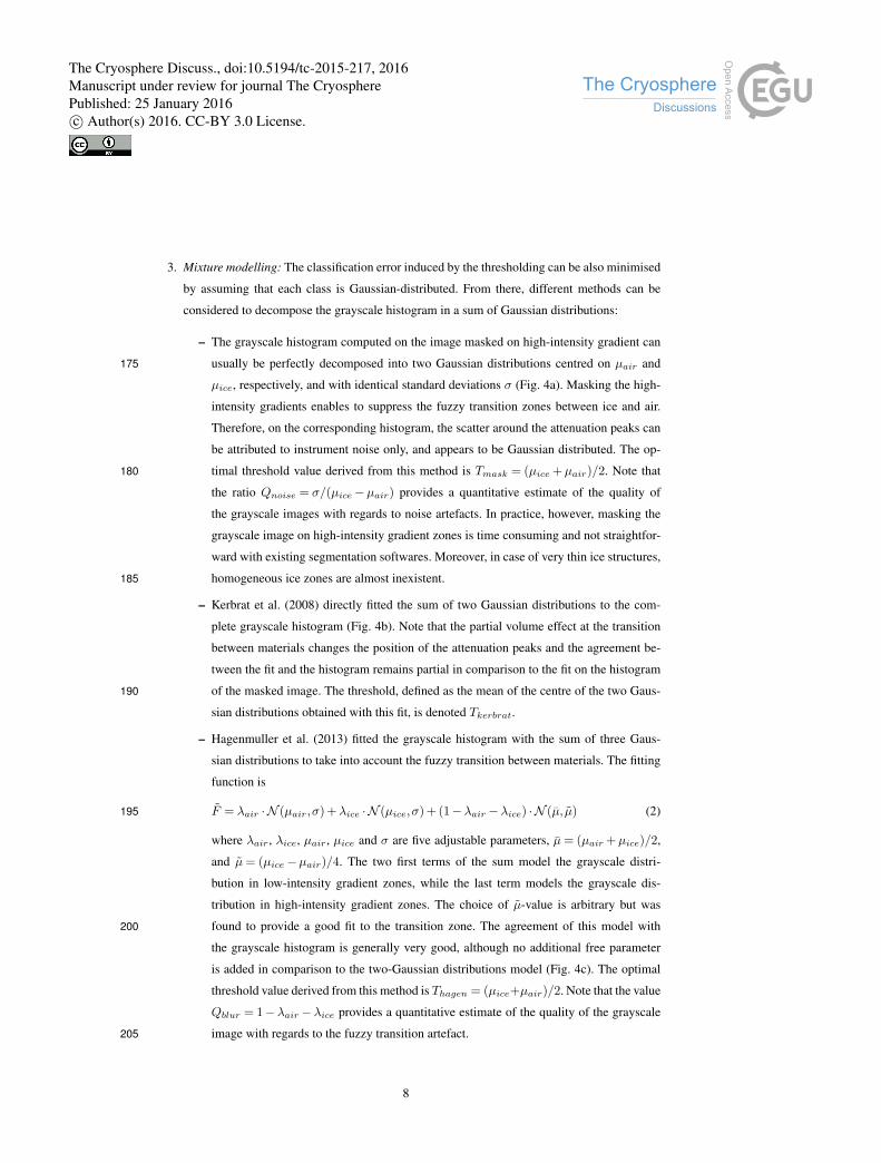
– The grayscale histogram computed on the image masked on high-intensity gradient can
usually be perfectly decomposed into two Gaussian distributions centred on µair and175
µice, respectively, and with identical standard deviations σ (Fig. 4a). Masking the high-
intensity gradients enables to suppress the fuzzy transition zones between ice and air.
Therefore, on the corresponding histogram, the scatter around the attenuation peaks can
be attributed to instrument noise only, and appears to be Gaussian distributed. The op-
timal threshold value derived from this method is Tmask = (µice +µair)/2. Note that180
the ratio Qnoise = σ/(µice−µair) provides a quantitative estimate of the quality of
the grayscale images with regards to noise artefacts. In practice, however, masking the
grayscale image on high-intensity gradient zones is time consuming and not straightfor-
ward with existing segmentation softwares. Moreover, in case of very thin ice structures,
homogeneous ice zones are almost inexistent.185
– Kerbrat et al. (2008) directly fitted the sum of two Gaussian distributions to the com-
plete grayscale histogram (Fig. 4b). Note that the partial volume effect at the transition
between materials changes the position of the attenuation peaks and the agreement be-
tween the fit and the histogram remains partial in comparison to the fit on the histogram
of the masked image. The threshold, defined as the mean of the centre of the two Gaus-190
sian distributions obtained with this fit, is denoted Tkerbrat.
– Hagenmuller et al. (2013) fitted the grayscale histogram with the sum of three Gaus-
sian distributions to take into account the fuzzy transition between materials. The fitting
function is
F̃ = λair · N (µair,σ) +λice · N (µice,σ) + (1−λair −λice) · N (µ̄, µ̃) (2)195
where λair, λice, µair, µice and σ are five adjustable parameters, µ̄= (µair +µice)/2,
and µ̃= (µice−µair)/4. The two first terms of the sum model the grayscale distri-
bution in low-intensity gradient zones, while the last term models the grayscale dis-
tribution in high-intensity gradient zones. The choice of µ̃-value is arbitrary but was
found to provide a good fit to the transition zone. The agreement of this model with200
the grayscale histogram is generally very good, although no additional free parameter
is added in comparison to the two-Gaussian distributions model (Fig. 4c). The optimal
threshold value derived from this method is Thagen = (µice+µair)/2. Note that the value
Qblur = 1−λair −λice provides a quantitative estimate of the quality of the grayscale
image with regards to the fuzzy transition artefact.205
8
The Cryosphere Discuss., doi:10.5194/tc-2015-217, 2016Manuscript under review for journal The CryospherePublished: 25 January 2016c© Author(s) 2016. CC-BY 3.0 License.

34000 38000 42000Absorption level (arbitrary units)
Occ
uren
ce ra
tio
a)
Tmask
Init. hist.Masked hist.Pure airPure iceRecon. hist.
34000 38000 42000Absorption level (arbitrary units)
Occ
uren
ce ra
tio
b)
Tkerbrat
Init. hist.Pure airPure iceRecon. hist.
34000 38000 42000Absorption level (arbitrary units)
Occ
uren
ce ra
tio
c)
Thagen
Init. hist.Pure airPure iceFronteerRecon. hist.
Figure 4. Different intensity models based on the grayscale distribution. (a) Mixture model composed of two
Gaussian distributions to reproduce the grayscale distribution on the low-intensity gradient zones. L1 error is
0.006. (b) Mixture model composed of two Gaussian distributions to reproduce the whole grayscale distribution.
L1 error is 0.14. (c) Mixture model composed of three Gaussian distributions to reproduce the whole grayscale
distribution. L1 error is 0.03. For all figures, the L1 error is the integral of the absolute difference between the
measured and the modelled grayscale distribution. Note that the area under the grayscale distribution of the
entire image is 1.
Post-processing. In general, the binary segmented image needs to be further corrected to remove
remaining artefacts. This can be done manually for each 2D section, but it is extremely time-
consuming (Flin et al., 2003). The continuity of the ice matrix can also be used to correct the bi-
nary image by deleting ice zones not connected to the main structure or to the edges of the image
(Hagenmuller et al., 2013; Schleef et al., 2014; Calonne et al., 2014). Among generic and automatic210
post-processing methods, the morphological operators erosion and dilation are the most popular. The
combination of these operators enables to delete small holes in the ice matrix (closing: erosion then
dilation) or small protuberances on the ice surface (opening: dilation then erosion). In the following,
the support size if these morphological filters is denoted d.
2.2.2 Energy-based segmentation215
Energy-based segmentation methods consist in finding the optimal segmentation by minimising a
prescribed energy function. These methods are robust and flexible since the best segmentation is
automatically found by the optimisation process, and the energy function can incorporate various
segmentation criteria. In general, the optimisation of functions composed of billions of variables
can be complex and time-consuming. However, provided that the variables are binary and some220
additional restrictions on the form of the energy function, efficient global optimisation methods
exist. In particular, functions that involve only pair interactions can be globally optimised in a very
efficient way with the graph cut method (Kolmogorov and Zabih, 2004). Using this method, the
9
The Cryosphere Discuss., doi:10.5194/tc-2015-217, 2016Manuscript under review for journal The CryospherePublished: 25 January 2016c© Author(s) 2016. CC-BY 3.0 License.
34000 38000 42000Absorption level (arbitrary units)
Occ
uren
ce ra
tio
0.0
0.2
0.4
0.6
0.8
1.0
Pro
xim
ityHistogramProx. to air P0
Prox. to ice P1
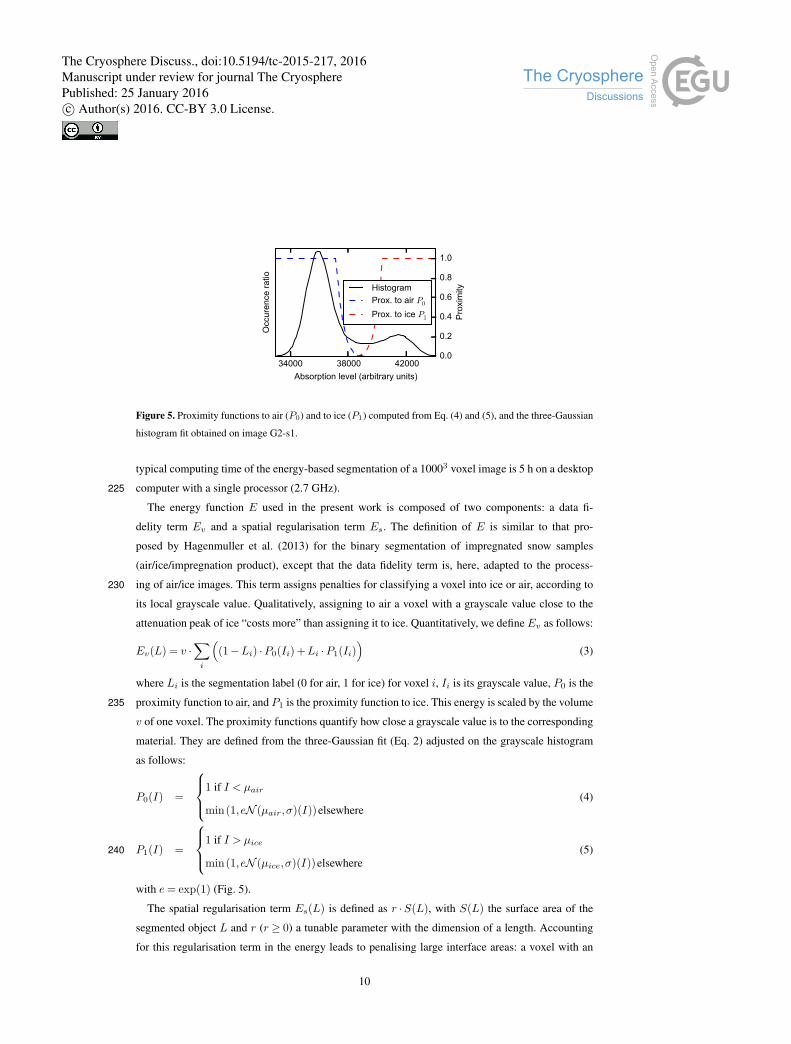
Figure 5. Proximity functions to air (P0) and to ice (P1) computed from Eq. (4) and (5), and the three-Gaussian
histogram fit obtained on image G2-s1.
typical computing time of the energy-based segmentation of a 10003 voxel image is 5 h on a desktop
computer with a single processor (2.7 GHz).225
The energy function E used in the present work is composed of two components: a data fi-
delity term Ev and a spatial regularisation term Es. The definition of E is similar to that pro-
posed by Hagenmuller et al. (2013) for the binary segmentation of impregnated snow samples
(air/ice/impregnation product), except that the data fidelity term is, here, adapted to the process-
ing of air/ice images. This term assigns penalties for classifying a voxel into ice or air, according to230
its local grayscale value. Qualitatively, assigning to air a voxel with a grayscale value close to the
attenuation peak of ice “costs more” than assigning it to ice. Quantitatively, we defineEv as follows:
Ev(L) = v ·∑
i
((1−Li) ·P0(Ii) +Li ·P1(Ii)
)(3)
where Li is the segmentation label (0 for air, 1 for ice) for voxel i, Ii is its grayscale value, P0 is the
proximity function to air, and P1 is the proximity function to ice. This energy is scaled by the volume235
v of one voxel. The proximity functions quantify how close a grayscale value is to the corresponding
material. They are defined from the three-Gaussian fit (Eq. 2) adjusted on the grayscale histogram
as follows:
P0(I) =
1 if I < µair
min(1,eN (µair,σ)(I))elsewhere(4)
P1(I) =
1 if I > µice
min(1,eN (µice,σ)(I))elsewhere(5)240
with e= exp(1) (Fig. 5).
The spatial regularisation term Es(L) is defined as r ·S(L), with S(L) the surface area of the
segmented object L and r (r ≥ 0) a tunable parameter with the dimension of a length. Accounting
for this regularisation term in the energy leads to penalising large interface areas: a voxel with an
10
The Cryosphere Discuss., doi:10.5194/tc-2015-217, 2016Manuscript under review for journal The CryospherePublished: 25 January 2016c© Author(s) 2016. CC-BY 3.0 License.

intermediate gray value is segmented so that the interface air/ice area is minimised. The parameter245
r assigns a relative weight to the surface area term in the total energy function E, and can be in-
terpreted as the minimum radius of protuberances preserved on the segmented object (Hagenmuller
et al., 2013). This regularisation term minimising the ice/air interface is of particular interest for ma-
terials such as snow where metamorphism naturally tends to reduce the surface and grain boundary
energy. Such processes are known to be particularly effective on snow types resulting from isother-250
mal metamorphism. For other snow types, such as precipitation particles, faceted crystals or depth
hoar, the surface regularisation term is expected to perform well in recovering the facet shapes, but
may induce some rounding at facet edges.
2.3 Surface area computation
Flin et al. (2011) evaluated three different approaches to compute the area of the ice-pore interface255
from 3D binary images: the stereological approach (e.g. Torquato, 2002), the marching cubes ap-
proach (e.g. Hildebrand et al., 1999) and the voxel projection approach (Flin et al., 2005). These
authors showed that the three approaches provide globally similar results, but each possesses its
own inherent drawbacks: the stereological approach does not handle anisotropic structures properly,
the marching cubes tends to overestimate the surface, and the voxel projection method is highly260
sensitive to image resolution. In the present work, in order to estimate whether variations of SSA
due to different surface area computation approaches are significant compared to the effect of bi-
nary segmentation, we tested three different methods to quantify the surface area: the stereological
approach, the marching cubes approach and the Crofton approach. We did not evaluate the voxel
projection method (Flin et al., 2005) because its implementation is sophisticated and the required265
computation of high-quality normal vectors is excessively time-consuming if used only for surface
area computation.
2.3.1 Model based stereological approach
Stereological methods derive higher dimensional geometrical properties, as density or SSA, from
lower dimensional data. The key idea is to count the intersections of the reference material with270
points or lines. Prior to the development of X-ray tomography, so-called model based methods were
used. These models assume certain geometric properties of the object being studied, such as the
isotropy of the material (Edens and Brown, 1995). They are now replaced by design-based methods
that do not require any prior information on the studied object but require denser sampling of the
object (Baddeley and Vedel Jensen, 2005; Matzl and Schneebeli, 2010).275
Here, we used two variants of the stereological method by measuring the intersection of lines
in a 3D-volume. The first method was by counting the number of interface points on linear paths
aligned with the three orthogonal directions. The surface area is then twice the number of intersec-
tions times the area of a voxel face. A surface area value is obtained for each direction. With the
11
The Cryosphere Discuss., doi:10.5194/tc-2015-217, 2016Manuscript under review for journal The CryospherePublished: 25 January 2016c© Author(s) 2016. CC-BY 3.0 License.

microtomographic data presented in this paper, the 2D sections are virtual and do not correspond280
to physical surface sections of the sample. This corresponds to a model-based stereological method
since isotropy of the sample is assumed, we call it in the following "stereological".
In addition, we used the mathematical formalism provided by the Cauchy-Crofton formula that
explicitly relates the area of a surface to the number of intersections with any straight lines (Boykov
and Kolmogorov, 2003). Instead of using only three orthogonal directions of the straight lines, we285
used 13 and 49 directions, and the improved approximations based on Voronoi diagrams proposed
by Danek and Matula (2011). This method comes close to a design based stereological method, as
the volume (and direction) is almost exhaustively sampled. We refer to this area computation method
to as the Crofton approach.
2.3.2 Marching cubes approach290
The marching cubes approach consists in extracting a polygonal mesh of an isosurface from a three-
dimensional scalar field. Summing the area contributions of all polygons constituting the mesh pro-
vides the surface area of the whole image. We used a homemade version of the algorithm developed
by Lorensen and Cline (1987). It computes the area of the 0.5-isosurface of the binary image with-
out any further processing of the image. Our version of the algorithm is adapted to compute only the295
surface area without saving all the mesh elements that are required for 3D visualisation.
3 Results
In this section, the methods to compute the area of the ice-air interface are evaluated first, since
this evaluation can be performed on reference objects whose area is theoretically known, without
accounting for the interplay with the binary segmentation method. The Crofton approach, which is300
shown to perform best, is selected for the rest of the study. The sensitivity of density and SSA to
the parameters of the sequential filtering and energy-based segmentations on the entire set of snow
images is then investigated. Finally the variability of SSA due to numerical processing is compared
to the variability of SSA due to snow spatial heterogeneity and scanning resolution.
3.1 Surface area estimation305
An oblate spheroid (or ellipsoid of revolution) with symmetry axis along z was chosen as a reference
object to compare the different surface area computation methods. An anisotropy of 0.6 was consid-
ered (ratio between the dimensions of z- and (x,y)-semi-axes), and spheroids of different sizes were
used to evaluate the impact of the discretization on the surface area computation. Figure 6 shows that
the surface area calculated with the Crofton approach is in excellent agreement with the theoretical310
area: for sufficiently large spheroids, i.e. surface area larger than 200 voxels2, the relative error is
less than 1% for the Crofton approach with 49 different directions and 2% for the Crofton approach
12
The Cryosphere Discuss., doi:10.5194/tc-2015-217, 2016Manuscript under review for journal The CryospherePublished: 25 January 2016c© Author(s) 2016. CC-BY 3.0 License.

0 500 1000 1500 2000 2500 3000 3500Reference surface area of ellipsoid (voxel2 )
0.3
0.2
0.1
0.0
0.1
0.2
0.3
0.4
Rel
ativ
e er
ror
Crofton 13Crofton 49Marching cubesStereological zStereological yStereological xStereological mean
Figure 6. Surface area of an oblate spheroid, obtained with different calculation methods. The spheroid has
a horizontal (x, y) semi-axis a varying in [3,19] voxel and a vertical (z) semi-axis c= 0.6 · a. The reference
surface area of the spheroid is computed analytically. The Crofton approach is computed with 13 or 49 different
directions. As in Fig. 10, 11, 12 and 13, the relative error is calculated as the computed value minus the reference
value, divided by the reference value.
with 13 different directions. Adding more directions does not significantly improve the accuracy of
the Crofton approach while it increases the computation time. The marching cubes approach system-
atically overestimates the surface area by about 5% due to the presence of artificial stair-steps in the315
triangulation of the isosurface. As expected, the stereological method shows scatter in the results ob-
tained between the z- and the (x,y) components. The mean value of the three components provides
a fair estimation of the surface area with a relative error of about 2% compared to the theoretical
value. These observations on the stereological and marching cubes approaches corroborate previous
results obtained by Flin et al. (2011) on snow images.320
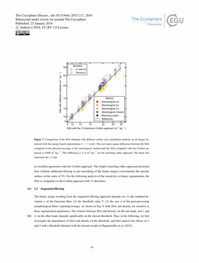
The different surface area computation methods were then evaluated on the entire set of snow
images segmented with the energy-based method (r = 1). According to the results obtained on the
spheroid, the Crofton approach with 13 directions was chosen as a reference. As shown in Fig. 7,
the SSA obtained with the direction-averaged stereological method is in excellent agreement with
the value provided by the Crofton method. The results of the marching cubes method are in fair325
agreement but show a systematic over-estimation of the SSA (+6% average relative deviation).
In summary, all presented area computation method showed consistent results. The Crofton ap-
proach showed the best accuracy on an artificial anisotropic structure whose surface area is theoret-
ically known. The stereological approach is negatively affected by strong anisotropy of the imaged
structure. However on the tested snow images, the structural anisotropy is low and this method is330
13
The Cryosphere Discuss., doi:10.5194/tc-2015-217, 2016Manuscript under review for journal The CryospherePublished: 25 January 2016c© Author(s) 2016. CC-BY 3.0 License.
9 10 12 15 20 25 30SSA with the 13 directions Crofton approach (m2 kg−1 )
9
10
12
15
20
25
30
SS
A w
ith d
iffer
ent m
etho
ds (m
2 k
g−1)
MethodStereological (z)Stereological (y)Stereological (x)Stereological (mean)Marching cubesReference
Sampless1 and s210micron
Sampless1 and s210micron
Figure 7. Comparison of the SSA obtained with different surface area calculation methods on all images bi-
narized with the energy-based segmentation (r = 1 voxel). The root mean square difference between the SSA
computed as the direction-average of the stereological method and the SSA computed with the Crofton ap-
proach is 0.008 m2 kg−1. This difference is 1.13 m2 kg−1 for the marching cubes approach. The black line
represents the 1:1 line.
in excellent agreement with the Crofton approach. The simple marching cubes approach presented
here (without additional filtering or pre-smoothing of the binary image) overestimates the specific
surface on the order of 5%. For the following analysis of the sensitivity to binary segmentation, the
SSA is computed via the Crofton approach with 13 directions.
3.2 Sequential filtering335
The binary image resulting from the sequential filtering approach depends on: (1) the standard de-
viation σ of the Gaussian filter, (2) the threshold value T , (3) the size d of the post-processing
morphological filters (opening/closing). As shown in Fig. 8, both SSA and density are sensitive to
these segmentation parameters. The relation between SSA and density, on the one hand, and σ and
d, on the other hand, depends significantly on the chosen threshold. Thus, in the following, we first340
investigate the dependence of SSA and density on the threshold, and then analyse the effects of σ
and d with a threshold obtained with the mixture model of Hagenmuller et al. (2013).
14
The Cryosphere Discuss., doi:10.5194/tc-2015-217, 2016Manuscript under review for journal The CryospherePublished: 25 January 2016c© Author(s) 2016. CC-BY 3.0 License.

120 140 160 180 200 220Density (kg m−3 )
23
24
25
26
27
28
29
30
Spe
cific
sur
face
are
a (m
2 k
g−1)
Gaussian filter size σ00.50.8
0.91.01.1
1.21.52.0
Threshold TValleyOtsu
KerbratHagenmuller
Morphological filter size d0.01.0
1.51.9
2.0
Figure 8. SSA and density of image G2-s1 obtained with sequential filtering for different segmentation param-
eters.
3.2.1 Choice of threshold
The threshold Tmask obtained with the two-Gaussian fit of the grayscale histogram computed on
the low-intensity gradient zones is chosen as a reference since this value is not affected by the345
fuzzy transition artefact. This reference threshold ranges between 38800 and 39500 for the different
scanned images (Fig. 9). The mean values of the attenuation peaks of air and ice are µair = 35800
and µice = 42600, respectively. Hence, the variations of the reference threshold value remain small
compared to the contrast between the two attenuation peaks µice−µair = 6800. However, these
variations clearly indicate, once again, that a unique threshold value cannot be used for all images.350
These variations could be explained by slight variations in the X-ray source energy level due to slight
temperature changes, or to deviations from the Beer-Lambert attenuation law depending on the total
ice content of the sample.
As shown in Fig. 9, the computed threshold depends significantly on the determination method.
These variations affect in turn the density extracted from the binary image (Fig. 10a). Note that the355
scatter on density due to the choice of the threshold remains the same even if a Gaussian filter is
applied on the grayscale image before thresholding (Fig. 10a). The SSA values are also affected
by the threshold determination method, but to a smaller extent since the threshold value tends to
15
The Cryosphere Discuss., doi:10.5194/tc-2015-217, 2016Manuscript under review for journal The CryospherePublished: 25 January 2016c© Author(s) 2016. CC-BY 3.0 License.

affect density and total surface area in the same proportion (Fig. 10b). The variation of SSA due to
smoothing is much more important than those due to the choice of the threshold (Fig. 10b).360
In detail, the valley method systematically overestimates the threshold value, leading to a sys-
tematic underestimation of the snow density by about 10 kg m−3 on average. Otsu’s method tends
to underestimate the threshold value, leading to an overestimation of the snow density by about
6 kg m−3 on average. Kerbrat’s method tends to underestimate the threshold value, leading to an
overestimation of the snow density by about 4 kg m−3 on average. Note that the density overestima-365
tion with Kerbrat’s method is more pronounced on low-density snow samples scanned with a 18 µm
resolution. Lastly, the method introduced by Hagenmuller et al. (2013) slightly underestimates the
threshold value, and therefore overestimates the snow density with a mean absolute difference of
about 2 kg m−3 compared to the reference.
In summary, the threshold value obtained with the valley method, a method widely used in the370
snow community, clearly leads to an underestimation of snow density. The mixture models of Ker-
brat et al. (2008) or Hagenmuller et al. (2013), which assume that noise is Gaussian distributed,
provide a threshold value in good agreement with the reference method. The model of Hagenmuller
et al. (2013), which explicitly accounts for the fuzzy transition between materials, yields the thresh-
old which is the closest to the reference value obtained on the masked image.375
3.2.2 Gaussian filtering
The sensitivity of density and surface area to the standard deviation σ of the Gaussian smoothing
kernel is shown on Fig. 11. The segmentation was performed with the threshold Thagen derived with
the method of Hagenmuller et al. (2013).
Depending on the sample, density varies in the range [-8, +2]% (compared to the value obtained380
without smoothing) when σ is increased from 0 to 20 µm (Fig. 11a). Density appears to be insensitive
to σ when σ is much lower than the voxel size. For larger values of σ, an average decrease of density
with σ is observed due to the fact that snow structure is generally convex and smoothing tends to
erode convex zones. Slight increase of density with σ is observed for σ > 5 µm for samples M1-1,
M1-3 and M2-2. These samples are the most faceted snow samples exhibiting a large proportion of385
flat surfaces (Fig. 1), which explains the different variation of density with σ. Systematic differences
can also be noted between the images with a resolution of 10 µm and 18 µm. At a resolution of
10 µm, a fast decrease of density is observed for σ in the range [3, 6] µm. This regime is absent
at a resolution of 18 µm. For larger values of σ, the evolution of density is then similar for the two
resolutions, and depends on the snow type. This difference is attributable to a stronger noise in the390
10 µm images, which results in local grayscale variations that are generally smoothed out when
σ > 6 µm.
The computed surface area significantly decreases when σ increases (Fig. 11b). Relative variations
up to 50% are observed. On the 10 µm images and with σ in the range [3, 6] µm, the surface
16
The Cryosphere Discuss., doi:10.5194/tc-2015-217, 2016Manuscript under review for journal The CryospherePublished: 25 January 2016c© Author(s) 2016. CC-BY 3.0 License.

38600 39000 39400 39800Reference threshold (arbitrary units)
38600
38800
39000
39200
39400
39600
39800
Thre
shol
d (a
rbitr
ary
units
)
MethodTvalleyTotsuTkerbratThagen
Sampless1 and s210micron
Sampless1 and s210micron
-8
-6
-4
-2
0
2
4
6
8
Sca
led
thre
shol
d 10
0·(T−T)/
( µice−µair)
(%)
-8 -6 -4 -2 0 2 4 6 8Scaled threshold 100 ·(T−T)/(µice−µair) (%)
Figure 9. Sequential filtering segmentation: threshold values obtained on the entire set of images with the
different intensity models. The black line represents the 1:1 line. The obtained thresholds T are also expressed
as a function of the mean threshold T and the mean contrast µice −µairbetween air and ice, obtained with the
reference method.
area decreases rapidly when σ increases. These variations probably correspond to the progressive395
smoothing of noise-induced fluctuations on the interface. For larger values of σ, the surface area
decreases much more slowly, which corresponds to the progressive smoothing of real microstructural
details. On the 18 µm images, these two regimes cannot be distinguished because the overall surface
area is less affected by noise artefacts and only the smoothing of real structural details is observed.
The same variations with σ can be observed on SSA since the variations of density with σ are small400
compared to the variations of the surface area. Note that the absolute values of density and SSA for
the different scanned snow images are indicated on Fig. 15.
3.2.3 Morphological opening/closing
Figure 12 shows the relative variation of density and surface area obtained with morphological filters
of different sizes d. Note that the values of d are constrained by the voxel grid and are thus discrete405
(1,√
2,√
3, 2 voxel, etc.). The opening and closing filters delete holes in the ice matrix or ice
elements in the air, of a typical size d. Therefore, the surface area decreases when d increases.
Density, on the contrary, is not very sensitive to d. When no Gaussian filter is applied to the grayscale
17
The Cryosphere Discuss., doi:10.5194/tc-2015-217, 2016Manuscript under review for journal The CryospherePublished: 25 January 2016c© Author(s) 2016. CC-BY 3.0 License.

200 220 240 260 280 300 320 340 360Reference density (kg m−3 )
0.10
0.05
0.00
0.05
0.10
0.15
Rel
ativ
e di
ffere
nce
of d
ensi
ty
a)
Sampless1 and s210micron
Sampless1 and s210micron
10 15 20 25 30 35 40 45Reference SSA (m2 kg−1 )
0.10
0.05
0.00
0.05
0.10
0.15
Rel
ativ
e di
ffere
nce
of S
SA
b)
MethodTvalley
Totsu
Tkerbrat
Thagen
MethodTvalley
Totsu
Tkerbrat
Thagen
Figure 10. Sequential filtering segmentation: relative variation of density (a) and SSA (b) computed with dif-
ferent threshold-determination methods, with respect to the reference values computed with Tmask. Void (re-
spectively solid) markers correspond to values obtained without any smoothing (respectively with a Gaussian
filter of standard deviation σ = 1 voxel). The legends apply to both subplots.
0 5 10 15 20σ (µm)
0.10
0.08
0.06
0.04
0.02
0.00
0.02
Rel
ativ
e di
ffere
nce
of d
ensi
ty
a)
Sampless1 and s210micron
Sampless1 and s210micron
0 5 10 15 20σ (µm)
0.6
0.5
0.4
0.3
0.2
0.1
0.0
0.1
Rel
ativ
e di
ffere
nce
of s
urfa
ce a
rea
b)
Figure 11. Sequential filtering segmentation: relative variations of density (a) and surface area (b) with the size
σ of the Gaussian filter. The variations are calculated with respect to density and surface area obtained without
smoothing filter (σ = 0).
18
The Cryosphere Discuss., doi:10.5194/tc-2015-217, 2016Manuscript under review for journal The CryospherePublished: 25 January 2016c© Author(s) 2016. CC-BY 3.0 License.

0.0 0.5 1.0 1.5 2.0d (voxel)
0.10
0.08
0.06
0.04
0.02
0.00
0.02
Rel
ativ
e di
ffere
nce
of d
ensi
ty
a)
Sampless1 and s210micron
Sampless1 and s210micron
0.0 0.5 1.0 1.5 2.0d (voxel)
0.5
0.4
0.3
0.2
0.1
0.0
0.1
Rel
ativ
e di
ffere
nce
of s
urfa
ce a
rea
b)
Smoothing (voxel)σ=0
σ=0.5
σ=1.0
Smoothing (voxel)σ=0
σ=0.5
σ=1.0
Figure 12. Sequential filtering segmentation: relative variations of density (a) and surface area (b) as a function
of the morphological filter size d for different values of the Gaussian filter size σ. The legends apply to both
subplots.
image, thresholding yields a lot of small details in the binary image, which enhances the effect of
morphological filters (Fig. 12b). When the image is already smoothed by Gaussian filtering, the410
morphological filters have less effect on the overall density and specific surface area. However, note
that using a Gaussian filter of standard deviation σ does not guarantee the complete absence of
details “smaller” than σ. Certain algorithms based on the binary images, such as grain segmentation
(e.g. Theile and Schneebeli, 2011; Hagenmuller et al., 2014) are highly sensitive to the presence of
residual artefacts in the ice matrix and require the use of these additional morphological filters.415
3.3 Energy-based approach
The binary image image resulting from the energy-based approach depends on the parameter r which
controls the smoothness of the segmented object. The other parameters involved in the volumetric
term Ev of the segmentation energy are directly derived from the three Gaussian mixture model (see
Sect. 2.2.1).420
As shown in Fig. 13a, the density of the segmented object slightly varies with r. On the 10 µm
images, the evolution of density with r is not monotonic but relative variations remain limited in
the range [-4, +1]%. On the 18 µm images, density clearly decreases when σ increases. This higher
sensitivity of density to r on the 18 µm images can be explained by the fact that the fuzzy transition
appears to be larger than on the 10 µm images, which leads to a higher indetermination of the exact425
position of the interface between ice and air in this moderate intensity gradient zone (Fig. 14).
19
The Cryosphere Discuss., doi:10.5194/tc-2015-217, 2016Manuscript under review for journal The CryospherePublished: 25 January 2016c© Author(s) 2016. CC-BY 3.0 License.
0 5 10 15 20r (µm)
0.10
0.08
0.06
0.04
0.02
0.00
0.02
Rel
ativ
e di
ffere
nce
of d
ensi
ty
a)
Sampless1 and s210micron
0 5 10 15 20r (µm)
0.5
0.4
0.3
0.2
0.1
0.0
0.1
Rel
ativ
e di
ffere
nce
of s
urfa
ce a
rea
b)
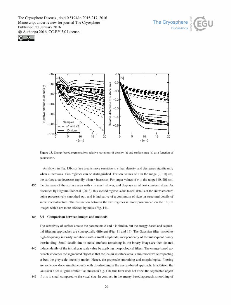
Figure 13. Energy-based segmentation: relative variations of density (a) and surface area (b) as a function of
parameter r.
As shown in Fig. 13b, surface area is more sensitive to r than density, and decreases significantly
when r increases. Two regimes can be distinguished. For low values of r in the range [0, 10] µm,
the surface area decreases rapidly when r increases. For larger values of r in the range [10, 20] µm,
the decrease of the surface area with r is much slower, and displays an almost constant slope. As430
discussed by Hagenmuller et al. (2013), this second regime is due to real details of the snow structure
being progressively smoothed out, and is indicative of a continuum of sizes in structural details of
snow microstructure. The distinction between the two regimes is more pronounced on the 10 µm
images which are more affected by noise (Fig. 14).
3.4 Comparison between images and methods435
The sensitivity of surface area to the parameters σ and r is similar, but the energy-based and sequen-
tial filtering approaches are conceptually different (Fig. 11 and 13). The Gaussian filter smoothes
high-frequency intensity variations with a small amplitude, independently of the subsequent binary
thresholding. Small details due to noise artefacts remaining in the binary image are then deleted
independently of the initial grayscale value by applying morphological filters. The energy-based ap-440
proach smoothes the segmented object so that the ice-air interface area is minimised while respecting
at best the grayscale intensity model. Hence, the grayscale smoothing and morphological filtering
are somehow done simultaneously with thresholding in the energy-based approach. In addition, the
Gaussian filter is “grid-limited”: as shown in Fig. 11b, this filter does not affect the segmented object
if σ is to small compared to the voxel size. In contrast, in the energy-based approach, smoothing of445
20
The Cryosphere Discuss., doi:10.5194/tc-2015-217, 2016Manuscript under review for journal The CryospherePublished: 25 January 2016c© Author(s) 2016. CC-BY 3.0 License.

0.12 0.14 0.16 0.18 0.20 0.22 0.24 0.26 0.28Qnoise
0.05
0.10
0.15
0.20
Qblur
Sampless1 and s210micron
Figure 14. Relative importance of the artefacts due to noise (Qnoise) and to the fuzzy transition (Qblur).Qnoise
corresponds to the ratio between the standard deviation of the Gaussian distributions fitted on the attenuation
peaks and the difference between the peak attenuation intensity of ice and air (see Sect. 2.2.1). Qblur corre-
sponds to the area of the Gaussian representing the fuzzy transition in Hagenmuller’s mixture model (see Sect.
2.2.1).
the ice-air interface occurs even for very low values of r (Fig. 13b) because voxels with a grayscale
value close to the threshold between ice and air can be segmented as air or ice without much change
in the data fidelity term Ev but with a clear change in the surface term Es. The parameter r defines
the largest equivalent spherical radius of details preserved in the segmented image, whereas σ does
not directly correspond to the size of the smallest detail.450
Figure 15 shows density and specific surface area computed on the entire set of snow images
segmented with the sequential filtering approach (σ = 1.0 voxel, T = Thagen, d= 1.0 voxel) and the
energy-based approach (r = 1.0 voxel). The “smoothing” parameters (σ and r) were chosen equal to
1.0 voxel since this value roughly corresponds to the transition beyond which the computed surface
area starts to vary slowly with σ and r (Fig. 11b, 13b), and therefore provides the segmentations455
that best preserve the smallest snow details while deleting most of noise-induced protuberances. As
already pointed out, this transition is clear on the 10 µm images, but less evident on the 18 µm
images. To be consistent, however, and to ensure that all noise artefacts are smoothed out, values of
r,σ = 1 voxel were used in all cases.
It is observed that the two approaches generally produce similar results in terms of density (root460
mean square deviation between the two segmentation methods is 6 kg m−3) and specific surface area
(root mean square deviation of 0.7 m2 kg−1). The largest differences are observed for the snow types
presenting the highest SSA. In general, the density provided by the sequential filtering is slightly
larger than that computed with the energy-based approach. The opposite difference is observed for
SSA.465
21
The Cryosphere Discuss., doi:10.5194/tc-2015-217, 2016Manuscript under review for journal The CryospherePublished: 25 January 2016c© Author(s) 2016. CC-BY 3.0 License.

Scatter can be observed even between the density and SSA derived from images coming from the
same snow block, due probably to the existence of spatial heterogeneities with the blocks and and the
difference of image quality. The averages of standard deviations calculated for each snow block are
10.7 kg m−3 and 1.1 m2 kg−1 for density and SSA, respectively (calculated with the energy-based
approach). This intra-block variability nevertheless appears to be limited compared to the inter-block470
variability (46.5 kg m−3 for density and 4.7 m2 kg−1, see Fig. 15), and is on the same order as the
variability due to the image processing technique (see above).
Lastly, systematically larger density and SSA values are found on the images scanned with a
10 µm resolution, compared to the images with a 18 µm resolution. It could be argued that this
difference is due to a better imaging of small details with a lower voxel size. However, as already475
noticed, the 10 µm images also present stronger noise artefacts (Fig. 14), and it is difficult to assess
whether the effective resolution of these images is, in practice, finer than the one of the 18 µm
images. Note that the root mean square difference between the density (respectively SSA) computed
on the images s1 and s2 is 3.8 kg m−3 (respectively 0.15 m2 kg−1), which is much lower than the
intra-block variability (including the 10 µm images). This observation indicates that the hardware480
setup of the tomograph and the subsequent image quality or resolution can significantly affect the
measured density and SSA.
4 Conclusions and discussions
We investigated the effect of numerical processing of microtomographic images on density and
specific surface area derived from these data. To this end, a set of 38 X-ray attenuation images of485
non-impregnated snow were analysed with different numerical methods to segment the grayscale
images and to compute the surface area on the resulting binary images.
The segmentation step is not straightforward because the grayscale images present noise and blur.
It is shown that noise artefacts can significantly affect the computed SSA, and that the fuzzy transi-
tion between ice and air can have a strong impact on the computed density.490
The sequential filtering approach critically depends on the threshold used to separate ice and air.
The grayscale histogram on low-intensity gradient zones presents two disjoint attenuation peaks,
whose characteristics are not affected by blur. The threshold derived from this method was used as
a reference to evaluate other methods based on the analysis of the grayscale histogram of the entire
image. The mixture models which consist in decomposing the histogram into a sum of Gaussian495
distributions are shown to be accurate. On the contrary, the local minimum method is shown to be
unsuitable in general.
Smoothing induced by the Gaussian and morphological filters in the sequential approach, or by
accounting for the surface area term in the energy-based method, efficiently remove noise artefacts
from the segmented binary image. Morphological filters applied on the binary image in the sequential500
22
The Cryosphere Discuss., doi:10.5194/tc-2015-217, 2016Manuscript under review for journal The CryospherePublished: 25 January 2016c© Author(s) 2016. CC-BY 3.0 License.

150 200 250 300 350 400 450Density (kg m−3 )
10
15
20
25
30
Spe
cific
sur
face
are
a (m
2 k
g−1)
A5B5C4D5-2D5E4F2G2H2M1-1M1-3M2N1Sequ. on s1 and s2Ener. on s1 and s2Sequ. on 10micronEner. on 10micron
Figure 15. Specific surface area as a function of density for the entire set of images and the two different binary
segmentation methods. The sequential filtering ("Sequ." in the legend) was applied with σ = 1.0 voxel, T =
Thagen and d= 1.0 voxel. The energy-based approach ("Ener." in the legend) was applied with r = 1.0 voxel.
The surface area was computed with the Crofton approach.
approach miss the initial gray value information. However, it seems that their effect is negligible if
the applied Gaussian filter is strong enough. The smoothing can also induce the disappearance of
real structural details contributing to the overall SSA. The transition between smoothing of noise
and smoothing of real details can be well estimated on the curve showing the evolution of SSA as a
function of σ or r. However, due to the influence of noise, it remains difficult to assess the potential505
contribution to the SSA of structural details of size smaller than the voxel size. It has previously been
shown that the SSA measured with gas adsorption technique, which has a molecular resolution, is
in good agreement with the SSA measured with microtomography for aged natural snow (Kerbrat
et al., 2008). This observation corroborates the idea that the surface of aged snow is smooth up to
a scale of about tens of microns, and that if smaller structures are present they do not contribute510
significantly to the overall SSA (Kerbrat et al., 2008). To further investigate this issue on recent
23
The Cryosphere Discuss., doi:10.5194/tc-2015-217, 2016Manuscript under review for journal The CryospherePublished: 25 January 2016c© Author(s) 2016. CC-BY 3.0 License.
snow and to disregard any additional influence of the measuring technique except the resolution, the
use of new tomographic systems with very high resolutions of about 1 µm would be necessary.
The formalism of the energy-based segmentation could enable to add more advanced criteria in the
segmentation process, such as the maximisation of the grayscale gradient at the segmented interface515
(Boykov and Jolly, 2001), the minimisation of the curvature of the segmented object (El-Zehiry and
Grady, 2010), or the spatial continuity in time-series of 3D images (Wolz et al., 2010). In this study,
only criteria on the local grayscale value and on the surface area of the segmented object were used.
The advantage of this method is that the parameter r formally defines an effective resolution of
the segmented image. In contrast, the standard deviation σ of the Gaussian smoothing kernel in the520
sequential approach does not explicitly define the smallest structural detail in the segmented image.
In practice, however, both methods provide very similar results on the tested images in terms of
density and SSA, provided appropriate parameters are chosen.
Comparison between the presented area computation methods showed similar results when ap-
plied to a synthetic image or to the set of snow images. On the synthetic image (oblate spheroid),525
the Crofton approach computes the surface area with highest accuracy (less than 2% for sufficiently
large spheroids) whereas the stereological approach is negatively affected by strong anisotropy of
the imaged structure and the unfiltered marching cubes approach overestimates the specific surface
on the order of 5%. Stereological methods using more complex test lines, such as a cycloids, can
compensate for the effect of anisotropy if the snow sample exhibits isotropy in a certain plane, which530
is often the case for the stratified snowpack (Matzl and Schneebeli, 2010). However on the tested
snow images, the surface anisotropy is low and the stereological method is in excellent agreement
with the Crofton approach. The unfiltered marching cubes approach still overestimates the specific
surface on the order of 5%. Note that methods have been developed to overcome this overestimation
problem of the marching cubes approach, such as the use of gray levels or smoothing (Flin et al.,535
2005). However, these methods may create other artefacts depending on the image considered, such
as systematic underestimation of the surface (Flin et al., 2005), and were not evaluated here.
The comparison of the sequential filtering and energy-based methods shows that density and SSA
can be estimated from X-ray tomography images with a “numerical” variability of the same order as
the variability due to spatial heterogeneities within one snow layer and to different hardware setups.540
5 Recommendations
A few recommendations to derive density and SSA from micro-tomographic data are summarized
below:
– Surface area computation. The unfiltered marching cubes approach systematically overesti-
mates the surface area and should thus be avoided. Counting intersections with test lines of545
24
The Cryosphere Discuss., doi:10.5194/tc-2015-217, 2016Manuscript under review for journal The CryospherePublished: 25 January 2016c© Author(s) 2016. CC-BY 3.0 License.

different orientations (at least in the three axes x, y and z) provides an efficient way to compute
the surface area and properly accounts for structural anisotropy.
– Threshold determination. The value of the threshold depends on the tomograph configura-
tion but also potentially on the scanned sample. A constant value for a time-series does not
necessarily prevent from density deviations due to beam hardening. Visual inspection of the550
histogram or the “valley method” do not always provide consistent threshold values. The fit
of Gaussian distributions on the histogram provides an automatic and satisfactory method to
determine an appropriate threshold value. However, all methods need visual inspection and
comparison with the grayscale image.
– Smoothing of grayscale image. Smoothing of the grayscale image, such as the convolution555
with a Gaussian kernel, is required to reduce noise artefacts but also reduces the effective
resolution of the image by deleting structural details that could contribute to the overall SSA.
The filter, and in particular the standard deviation σ of the applied Gaussian kernel, expressed
in µm, should be systematically mentioned if SSA values derived from tomographic data
are presented. Indeed, SSA is a decreasing function of the effective resolution even if the560
resolution is larger than the nominal voxel size. This function is expected to become constant
only for sufficiently small resolutions depending on the snow type.
25
The Cryosphere Discuss., doi:10.5194/tc-2015-217, 2016Manuscript under review for journal The CryospherePublished: 25 January 2016c© Author(s) 2016. CC-BY 3.0 License.

References
Baddeley, A. and Vedel Jensen, E. B.: Stereology for statisticians, Chapman & Hall/CRC, 2005.
Berthod, M., Kato, Z., Yu, S., and Zerubia, J.: Bayesian image classification using Markov random field, Image565
Vis. Comput., 14, 285–295, doi:10.1016/0262-8856(95)01072-6, 1996.
Boykov, Y. and Jolly, M.-P.: Interactive graph cuts for optimal boundary & region segmentation of objects in
ND images, Int. Conf. Comput. Vis., 1, 105–112, 2001.
Boykov, Y. and Kolmogorov, V.: Computing geodesics and minimal surfaces via graph cuts, in: Pro-
ceedings. Ninth IEEE Int. Conf. Comput. Vision, 2003, vol. 1, pp. 26–33, IEEE, Nice, France,570
doi:10.1109/ICCV.2003.1238310, 2003.
Brucker, L., Picard, G., Arnaud, L., Barnola, J.-M., Schneebeli, M., Brunjail, H., Lefebvre, E., and
Fily, M.: Modeling time series of microwave brightness temperature at Dome C, Antarctica, us-
ing vertically resolved snow temperature and microstructure measurements, J. Glaciol., 57, 171–182,
doi:10.3189/002214311795306736, 2011.575
Calonne, N., Flin, F., Geindreau, C., Lesaffre, B., and Roscoat, S. R. D.: Study of a temperature gradient
metamorphism of snow from 3-D images: time evolution of microstructures, physical properties and their
associated anisotropy, Cryosph. Discuss., 8, 1407–1451, doi:10.5194/tcd-8-1407-2014, 2014.
Cnudde, V. and Boone, M. N.: High-resolution X-ray computed tomography in geosciences: A review of the
current technology and applications, Earth-Science Rev., 123, 1–17, doi:10.1016/j.earscirev.2013.04.003,580
2013.
Coléou, C., Lesaffre, B., Brzoska, J.-B., Lüdwig, W., and Boller, E.: Three-dimensional snow images by X-ray
microtomography, Ann. Glaciol., 32, 75–81, doi:10.3189/172756401781819418, 2001.
Danek, O. and Matula, P.: On Euclidean Metric Approximation via Graph Cuts, in: Comput. Vision, Imaging
Comput. Graph. Theory Appl., edited by Richard, P. and Braz, J., vol. 229 of Communications in Computer585
and Information Science, pp. 125–134, Springer Berlin Heidelberg, Angers, France, doi:10.1007/978-3-642-
25382-9_9, 2011.
Domine, F., Taillandier, A.-S., and Simpson, W. R.: A parameterization of the specific surface area of
seasonal snow for field use and for models of snowpack evolution, J. Geophys. Res., 112, 1–13,
doi:10.1029/2006JF000512, 2007.590
Ebner, P. P., Schneebeli, M., and Steinfeld, A.: Tomography-based monitoring of isothermal snow metamor-
phism under advective conditions, The Cryosphere, 9, 1363–1371, doi:10.5194/tc-9-1363-2015, 2015.
Edens, M. and Brown, R. L.: Measurement of microstructure of snow from surface sections, Def. Sci. J., 45,
107–116, 1995.
El-Zehiry, N. and Grady, L.: Fast global optimization of curvature, IEEE Conf. Comput. Vis. Pattern Recognit.,595
pp. 3257–3264, doi:10.1109/CVPR.2010.5540057, 2010.
Fierz, C., Durand, R., Etchevers, Y., Greene, P., McClung, D. M., Nishimura K, Satyawali, P. K., and Sokra-
tov, S. A.: The international classification for seasonal snow on the ground, Tech. rep., IHP-VII Technical
Documents in Hydrology N83, IACS Contribution N1, UNESCO-IHP, Paris, 2009.
Flanner, M. G. and Zender, C. S.: Linking snowpack microphysics and albedo evolution, J. Geophys. Res., 111,600
D12 208, doi:10.1029/2005JD006834, 2006.
26
The Cryosphere Discuss., doi:10.5194/tc-2015-217, 2016Manuscript under review for journal The CryospherePublished: 25 January 2016c© Author(s) 2016. CC-BY 3.0 License.

Flin, F.: Snow metamorphism description from 3D images obtained by X-ray microtomography, Ph.D. thesis,
Université de Grenoble 1, 2004.
Flin, F., Brzoska, J.-B., Lesaffre, B., Coléou, C., and Pieritz, R. A.: Full three-dimensional modelling of
curvature-dependent snow metamorphism: first results and comparison with experimental tomographic data,605
J. Phys. D. Appl. Phys., 36, A49–A54, doi:10.1088/0022-3727/36/10A/310, 2003.
Flin, F., Brzoska, J.-B., Lesaffre, B., Coléou, C., and Pieritz, R. A.: Three-dimensional geometric mea-
surements of snow microstructural evolution under isothermal conditions, Ann. Glaciol., 38, 39–44,
doi:10.3189/172756404781814942, 2004.
Flin, F., Budd, W. F., Coeurjolly, D., Pieritz, R. A., Lesaffre, B., Coléou, C., Lamboley, P., Teytaud, F., Vi-610
gnoles, G. L., and Delesse, J.-F.: Adaptive estimation of normals and surface area for discrete 3-D ob-
jects: application to snow binary data from X-ray tomography, Image Process. IEEE Trans., 14, 585–596,
doi:10.1109/TIP.2005.846021, 2005.
Flin, F., Lesaffre, B., Dufour, A., Gillibert, L., Hasan, A., Roscoat, S. R. D., Cabanes, S., and Pugliese, P.: On
the Computations of Specific Surface Area and Specific Grain Contact Area from Snow 3D Images, in: Phys.615
Chem. Ice, edited by Furukawa, Y., pp. 321–328, Sapporo, Japan, 2011.
Hagenmuller, P., Chambon, G., Lesaffre, B., Flin, F., and Naaim, M.: Energy-based binary segmentation of
snow microtomographic images, J. Glaciol., 59, 859–873, doi:10.3189/2013JoG13J035, 2013.
Hagenmuller, P., Chambon, G., Flin, F., Morin, S., and Naaim, M.: Snow as a granular material: assessment of
a new grain segmentation algorithm, Granul. Matter, 16, 421–432, doi:10.1007/s10035-014-0503-7, 2014.620
Haussener, S.: Tomography-based determination of effective heat and mass transport properties of complex
multi-phase media, Ph.D. thesis, ETH Zürich, http://e-collection.library.ethz.ch/view/eth:2424, 2010.
Heggli, M., Frei, E., and Schneebeli, M.: Snow replica method for three-dimensional X-ray microtomographic
imaging, J. Glaciol., 55, 631–639, doi:10.3189/002214309789470932, 2009.
Hildebrand, T., Laib, A., Müller, R., Dequeker, J., and Rüegsegger, P.: Direct three-dimensional morphometric625
analysis of human cancellous bone: microstructural data from spine, femur, iliac crest, and calcaneus, J. bone
Miner. Res., 14, 1167–1174, doi:10.1359/jbmr.1999.14.7.1167, 1999.
Iassonov, P., Gebrenegus, T., and Tuller, M.: Segmentation of X-ray computed tomography images of porous
materials: A crucial step for characterization and quantitative analysis of pore structures, Water Resour. Res.,
45, W09 415, doi:10.1029/2009WR008087, 2009.630
Kaestner, A., Lehmann, E., and Stampanoni, M.: Imaging and image processing in porous media research, Adv.
Water Resour., 31, 1174–1187, doi:10.1016/j.advwatres.2008.01.022, 2008.
Kerbrat, M., Pinzer, B. R., Huthwelker, T., Gäggeler, H. W., Ammann, M., and Schneebeli, M.: Measuring the
specific surface area of snow with X-ray tomography and gas adsorption: comparison and implications for
surface smoothness, Atmos. Chem. Phys., 8, 1261–1275, doi:10.5194/acp-8-1261-2008, 2008.635
Kolmogorov, V. and Zabih, R.: What energy functions can be minimized via graph cuts?, IEEE Trans. Pattern
Anal. Mach. Intell., 26, 147–59, doi:10.1109/TPAMI.2004.1262177, 2004.
Lomonaco, R., Albert, M., and Baker, I.: Microstructural evolution of fine-grained layers through the firn col-
umn at Summit, Greenland, J. Glaciol., 57, 755–762, doi:10.3189/002214311797409730, 2011.
Lorensen, W. E. and Cline, H. E.: Marching Cubes: A High Resolution 3D Surface Construction Algorithm,640
SIGGRAPH Comput. Graph., 21, 163–169, doi:10.1145/37402.37422, 1987.
27
The Cryosphere Discuss., doi:10.5194/tc-2015-217, 2016Manuscript under review for journal The CryospherePublished: 25 January 2016c© Author(s) 2016. CC-BY 3.0 License.
Matzl, M. and Schneebeli, M.: Stereological measurement of the specific surface area of seasonal snow types:
Comparison to other methods, and implications for mm-scale vertical profiling, Cold Reg. Sci. Technol., 64,
1–8, doi:10.1016/j.coldregions.2010.06.006, 2010.
Otsu, N.: A threshold selection method from gray-level histograms, Automatica, 20, 62–66,645
doi:10.1109/TSMC.1979.4310076, 1975.
Pinzer, B. R., Schneebeli, M., and Kaempfer, T. U.: Vapor flux and recrystallization during dry snow metamor-
phism under a steady temperature gradient as observed by time-lapse micro-tomography, The Cryosphere,
6, 1141–1155, doi:10.5194/tc-6-1141-2012, 2012.
Riche, F., Schreiber, S., and Tschanz, S.: Design-based stereology to quantify structural proper-650
ties of artificial and natural snow using thin sections, Cold Reg. Sci. Technol., 79-80, 67–74,
doi:10.1016/j.coldregions.2012.03.008, 2012.
Schleef, S. and Löwe, H.: X-ray microtomography analysis of isothermal densification of new snow under
external mechanical stress, J. Glaciol., 59, 233–243, doi:10.3189/2013JoG12J076, 2013.
Schleef, S., Löwe, H., and Schneebeli, M.: Hot-pressure sintering of low-density snow analyzed by X-ray mi-655
crotomography and in situ microcompression, Acta Mater., 71, 185–194, doi:10.1016/j.actamat.2014.03.004,
2014.
Schlüter, S. and Sheppard, A.: Image processing of multiphase images obtained via X-ray microtomography: A
review Steffen, Water Resour. Res., pp. 3615–3639, doi:10.1002/2014WR015256, 2014.
Sezgin, M. and Sankur, B.: Survey over image thresholding techniques and quantitative performance evaluation,660
J. Electron. Imaging, 13, 220, doi:10.1117/1.1631315, 2004.
Theile, T. and Schneebeli, M.: Algorithm to decompose three-dimensional complex structures at the necks:
tested on snow structures, Image Process. IET, 5, 132–140, doi:10.1049/iet-ipr.2009.0410, 2011.
Theile, T., Szabo, D., Luthi, A., Rhyner, H., and Schneebeli, M.: Mechanics of the Ski-Snow Contact, Tribol.
Lett., 36, 223–231, doi:10.1007/s11249-009-9476-9, 2009.665
Torquato, S.: Random heterogeneous materials: microstructure and macroscopic properties, vol. 16, Springer,
doi:10.1007/978-1-4757-6355-3, 2002.
Vetter, R., Sigg, S., Singer, H. M., Kadau, D., Herrmann, H. J., and Schneebeli, M.: Simulating isothermal aging
of snow, Eur. Lett., 89, 26 001, doi:10.1209/0295-5075/89/26001, 2010.
Warren, S.: Optical properties of snow, Rev. Geophys., 20, 67–89, doi:10.1029/RG020i001p00067, 1982.670
Wolz, R., Heckemann, R. A., Aljabar, P., Hajnal, J. V., Hammers, A., Lötjönen, J., and Rueckert, D.: Mea-
surement of hippocampal atrophy using 4D graph-cut segmentation: application to ADNI., Neuroimage, 52,
109–18, doi:10.1016/j.neuroimage.2010.04.006, 2010.
28
The Cryosphere Discuss., doi:10.5194/tc-2015-217, 2016Manuscript under review for journal The CryospherePublished: 25 January 2016c© Author(s) 2016. CC-BY 3.0 License.
Recommended

![TWO-STAGE FACIAL AGE PREDICTION USING GROUP-SPECIFIC FEATURES · with these age-related facial features [6,11]. Motivated by this, we argue that group-specic features in the specic](https://img.dokumen.tips/doc/110x75/5e83270b59f9ee232270829d/two-stage-facial-age-prediction-using-group-specific-with-these-age-related-facial.jpg)


![Sensitivity of soil moisture to terrain and snow cover at watershed to plot scales in the Rocky Mountain Front Range, Colorado, USA [Stephanie Kampf]](https://img.dokumen.tips/doc/110x75/554db399b4c905ff7a8b5442/sensitivity-of-soil-moisture-to-terrain-and-snow-cover-at-watershed-to-plot-scales-in-the-rocky-mountain-front-range-colorado-usa-stephanie-kampf.jpg)