SEMI-AUTOMATED CLOUD/SHADOW REMOVAL AND LAND COVER CHANGE DETECTION USING SATELLITE IMAGERY
A. K. Sah a, *, B. P. Sah a, K. Honji a, N. Kubo a, S. Senthil a aPASCO Corporation, 1-1-2 Higashiyama, Meguro-ku, Tokyo 153-0043, Japan - (ahwaas9539, bhpa_s5512, kiojin6937,
noabmu3604)@pasco.co.jp, [email protected]
Commission VII, WG VII/5
KEY WORDS: Satellite, Forestry, Land Cover, Classification, Change Detection, Semi-automation ABSTRACT: Multi-platform/sensor and multi-temporal satellite data facilitates analysis of successive change/monitoring over the longer period and there by forest biomass helping REDD mechanism. The historical archive satellite imagery, specifically Landsat, can play an important role for historical trend analysis of forest cover change at national level. Whereas the fresh high resolution satellite, such as ALOS, imagery can be used for detailed analysis of present forest cover status. ALOS satellite imagery is most suitable as it offers data with optical (AVNIR-2) as well as SAR (PALSAR) sensors. AVNIR-2 providing data in multispectral modes play due role in extracting forest information. In this study, a semi-automated approach has been devised for cloud/shadow and haze removal and land cover change detection. Cloud/shadow pixels are replaced by free pixels of same image with the help of PALSAR image. The tracking of pixel based land cover change for the 1995-2009 period in combination of Landsat and latest ALOS data from its AVNIR-2 for the tropical rain forest area has been carried out using Decision Tree Classifiers followed by un-supervised classification. As threshold for tree classifier, criteria of NDVI refined by reflectance value has been employed. The result shows all pixels have been successfully registered to the pre-defined 6 categories; in accordance with IPCC definition; of land cover types with an overall accuracy 80 percent.
* Corresponding author.
1. INTRODUCTION
Historical archive satellite imagery together with fresh one gives potentiality classifying time series Land cover (LC) of an area. LC is being used for national land planning since long and time series LC opens new applications, such as Reducing Emissions form Deforestation and forest Degradation (REDD or REDD+). Satellite Remote Sensing is a primary information source for LC and forest assessment as it provides images of wider areas relatively in a faster and cost-efficient manner. After the launch of Landsat 1 Satellite in 1972, several satellites (with both optical and Synthetic Aperture Radar (SAR) sensors) have been launched and trend is continuing at present as well as several planned to be launched in future and in due course spatial resolution has improved to a large extent. High resolution satellite, such as Advanced Land Observing Satellite (ALOS) provides Advanced Visible and Near Infrared Radiometer Type 2 (AVNIR-2) imagery (10m resolution) can be used for analysis of present forest cover status (Nonomura et al., 2010). However, presence of cloud, shadow, and haze in satellite imagery hamper LC classification and need to be treated. Treatment of all of them (cloud, shadow, and haze) together in different landscape including forest land is the big issue. There are some programs currently available for cloud, shadow, and haze but these are fragmented and lack of holistic approach that can treat all of them. Experimenting on simulated ALOS data, Hoan and Tateishi, 2008 have used Total Reflectance Radiance Index (TRRI) to separate cloud area. Further for
separating thin cloud ‘Cloud Soil Index (CSI)’ criterion has been mentioned as second step. Also, satellite based imageries from various platforms and optical sensors have been providing LC information since long, but extracting them correctly is challenging tasks. Employing decision tree classification scheme, Hansen et al., 2000 produced global land cover for which multi-temporal Advanced Very High Resolution Radiometer (AVHRR) metrics were used. Use of multi-temporal satellite data to produce single time land cover becomes complicated for REDD (or REDD+) which needs LC classifications from past, present, and future satellite imagery with minimum human intervention so that it can fulfil the required MRV (Measuring, Reporting and Verification) transparency. Considering the above issues, in this study we present a semi-automated approach for cloud/shadow and haze removal and LC change detection as a whole. The concept of LC used in this study is equivalent to Land Use (LU) mentioned in IPCC. Most of the image processing steps have been carried out using PASCO Tool™. This has been developed using Erdas Macro Language (EML) and thus works with Erdas Imagine© 1991-2009 ERDAS, Inc., software environment. The processing steps comparatively require less operator inputs and can classify large number of satellite imageries with desired accuracy for pixel based change detection including defined number of LC classes as per IPCC (Bickel et al., 2006).
International Archives of the Photogrammetry, Remote Sensing and Spatial Information Sciences, Volume XXXIX-B7, 2012 XXII ISPRS Congress, 25 August – 01 September 2012, Melbourne, Australia
335
2. STUDY AREA AND DATA
The area selected for this Study is the Lake Mai-Ndombe (about 380km North-east of the capital, Kinshasa) and its surroundings in Democratic Republic of the Congo. This area has good coverage of forest with cropland and grassland in patches. Three epochs satellite data; 1990, 2000, and 2010 were used in the analysis and their details are as follows: i) Landsat 5 Thematic Mapper (TM): Path 180/Row 062, dated 1995 February 19. ii) Landsat 7 Enhanced Thematic Mapper Plus (ETM+): Path 180/Row 062, dated 2002 May 5. iii) ALOS AVNIR-2: Path 278/Frame 3650, dated 2009 July 4. Landsat 5 TM and Landsat 7 ETM+ have 7 bands and spatial resolution bands 1 to 5 and 7 are 30m. ALOS AVNIR-2 has 4 bands with spatial resolution 10m. Analyzed area was equal to one ALOS AVNIR-2 scene. This area was covered by 4 scenes of ALOS Phased Array type L-band Synthetic Aperture Radar (PALSAR) (Path 600/Row 714, dated 2009 October 4; Path 601/Row 713 & 714, dated 2009 July 4; Path 602/Row 713, dated 2009 September 12.
3. METHODOLOGY
3.1 Semi-automated Cloud/Shadow, and Haze Identification and Removal
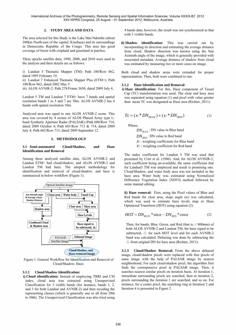
Among these analyzed satellite data, ALOS AVNIR-2 and Landsat ETM+ had cloud/shadow, and ALOS AVNIR-2 and Landsat TM had haze. The adopted methodology for identification and removal of cloud/shadow, and haze is summarized in below workflow (Figure 1). Figure 1. General Workflow for Identification and Removal of
Cloud/Shadow, Haze. 3.1.1 Cloud/Shadow Identification: i) Cloud identification: Instead of employing TRRI and CSI
index, cloud area was extracted using Unsupervised Classification for 3 visible bands (for instance, bands 1, 2, and 3 for both Landsat and AVNIR-2) and then recoding the representing classes (which is generally one or all from 28th to 30th). The Unsupervised Classification was also tried using
4 bands data; however, the result was not synchronized as that with 3 visible bands.
ii) Shadow identification: This was carried out by
incorporating its direction and estimating the average distance from cloud. Shadow direction was known using the Sun Azimuth angle of the image, which is generally provided with associated metadata. Average distance of shadow from cloud was estimated by measuring two or more cases on image.
Both cloud and shadow areas were extended for proper representation. Then, both were combined to one. 3.1.2 Haze Identification and Removal: i) Haze identification: For this, Haze component of Tassel
Cap (TC) transformation was used. The clear and hazy area was separated using equation (1) and pixel with value greater than mean TC was designated as Haze area (Richter, 2011).
)*()*( 21 REDBLUE DNxDNxTc += (1)
Where, BLUEDN : DN value in Blue band
REDDN : DN value in Red band 1x : weighing coefficients for Blue band 2x : weighing coefficient for Red band
The index coefficient for Landsat 5 TM was used that presented by Crist et al. (1986). And, for ALOS AVINIR-2, such coefficient being un-available, the same coefficient that for Landsat5 TM was employed and result is promising one. Cloud/Shadow, and water body area was not included in the haze area. Water body was estimated using Normalized Difference Vegetation Index (NDVI) method followed by some manual editing.
ii) Haze removal: First, using the Pixel values of Blue and Red bands for clear area, slope angle (α) was calculated, which was used to estimate haze levels map or Haze Optimized Transform (HOT) using equation (2).
αα cos*sin* REDBLUE DNDNHOT −= (2) Then, for bands; Blue, Green, and Red (that is, < 800mm) of both ALOS AVNIR-2 and Landsat TM, the haze signal to be subtracted, △ for each HOT level and for each AVNIR-2 band was calculated. Dehazing was done by subtracting the △ from original DN for haze area (Richter, 2011).
3.1.3 Cloud/Shadow Removal: From the above dehazed image, cloud/shadow pixels were replaced with free pixels of same image with the help of PALSAR image by nearest neighborhood. For each cloud/shadow pixel, the algorithm first finds the corresponsive pixel in PALSAR image. Then, it searches nearest similar pixels on iteration basis. At iteration 1, immediate surrounding pixels are searched, then at iteration 2, pixels surrounding the iteration 1 are searched, and so on. For instance, for a center pixel, the searching ring at Iteration 2 and Iteration 4 is presented in Figure 2.
Cloud area
Shadow area
Sun Azimuth angle& Average Cloud –Shadow Distance
Combined Cloud & Shadow area
Haze signal tobe subtracted, △
Dehazed Image
Cloud/Shadow, andHaze removed Image
Water body Tassel Cap
Clear area Haze area
Haze Levels
Optical Satellite Image
PALSAR Satellite Image
Cloud area
Shadow area
Sun Azimuth angle& Average Cloud –Shadow Distance
Combined Cloud & Shadow area
Haze signal tobe subtracted, △
Dehazed Image
Cloud/Shadow, andHaze removed ImageCloud/Shadow, andHaze removed Image
Water body Tassel Cap
Clear area Haze area
Haze Levels
Optical Satellite Image
PALSAR Satellite Image
International Archives of the Photogrammetry, Remote Sensing and Spatial Information Sciences, Volume XXXIX-B7, 2012 XXII ISPRS Congress, 25 August – 01 September 2012, Melbourne, Australia
336
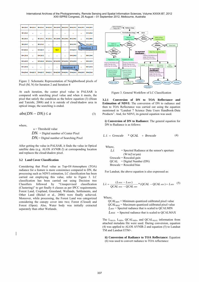
Figure 2. Schematic Representation of Neighborhood pixels of Pixel (M, N) for Iteration 2 and Iteration 4 At each iteration, the center pixel value in PALSAR is compared with searching pixel value and when it meets, the pixel that satisfy the condition as the below equation (3) (Hoan and Tateishi, 2008) and it is outside of cloud/shadow area in optical image, the searching is ended.
aDNDNabs ji ≤− )( (3) where, a = Threshold value iDN = Digital number of Center Pixel jDN = Digital number of Searching Pixel After getting the value in PALSAR, it finds the value in Optical satellite data (e.g. ALOS AVNIR-2) at corresponding location and replaces the cloud/shadow pixel. 3.2 Land Cover Classification
Considering that Pixel value as Top-Of-Atmosphere (TOA) radiance for a feature is more consistence compared to DN, the processing such as NDVI estimation, LC classification has been carried out employing this value, refer to Figure 3. LC classification has been carried out using Decision tree Classifiers followed by “Unsupervised classification (Clustering)” to get finally 6 classes as per IPCC requirements; Forest Land, Cropland, Grassland, Wetlands, Settlements, and Other Land (Bickel et al., 2006) were finally achieved. Moreover, while processing, the Forest Land was categorized considering the canopy cover into two; Forest (Closed) and Forest (Open). Also, Water body was initially extracted separately than other Wetlands.
Figure 3. General Workflow of LC Classification 3.2.1 Conversion of DN to TOA Reflectance and Estimation of NDVI: The conversion of DN to radiance and then to TOA Reflectance was carried out using the equation mentioned in “Landsat 7 Science Data Users Handbook-Data Products”. And, for NDVI, its general equation was used.
i) Conversion of DN to Radiance: The general equation for DN to Radiance is as follows:
BrescaleQCALGrescaleL += *λ (4)
Where, λL = Spectral Radiance at the sensor's aperture
(W/m2/sr/μm) Grescale = Rescaled gain QCAL = Digital Number (DN) Brescale = Rescaled bias
For Landsat, the above equation is also expressed as:
MINMINMINMAX
MINMAX LQCALQCALQCALQCALLLL +−
−−
= )(*)(λ (5)
Where, QCALMIN = Minimum quantized calibrated pixel value QCALMAX = Maximum quantized calibrated pixel value MINL = Spectral radiance that is scaled to QCALMIN MAXL = Spectral radiance that is scaled to QCALMAX The LMAX, LMIN, QCALMIN, and QCALMAX information from attached metadata file were used. During conversion, equation (4) was applied to ALOS AVNIR-2 and equation (5) to Landsat TM and Landsat ETM+.
ii) Conversion of Radiance to TOA Reflectance: Equation (6) was used to convert radiance to TOA reflectance:
Iteration 2
Iteration 4
Clipping TOA Reflectance image with this area, Clustering, & recoding
Clipping TOA Reflectance image with this area, Clustering, & recoding
Clipping TOA Reflectance image with this area, Clustering, & recoding
Un-supervisedClassification
Clipping TOA Reflectance image with this area, Clustering, & recoding
Un-supervisedClassification
NoYesNDVI of Non-Vegetation Area
- Forest (Closed)- Forest (Open)- Grassland (if present)
Land Use Classes:
Grassland Settlements/ Other Land
Other Land
Cropland
- Forest (Closed)- Forest (Open)- Grassland- Cropland (if present)
Land Use Classes:
NDVI > Threshold
NDVI of Vegetation Area
YesNo
NDVI of ‘Vegetation A’ Area
‘Vegetation A’ Area
Band 3(% reflectance)
Threshold
‘Vegetation B’ Area
Other Non-vegetation Area
SettlementsForest Land GrasslandCropland
Grassland
Optical SatelliteImage, DN
NDVI
Radiance Image
TOA Reflectance Image
No
NDVI > Threshold
NDVI > ThresholdYes
Yes
Other Wetlands
Water body
Wetlands
Clipping TOA Reflectance image with this area, Clustering, & recoding
Clipping TOA Reflectance image with this area, Clustering, & recoding
Clipping TOA Reflectance image with this area, Clustering, & recoding
Un-supervisedClassification
Clipping TOA Reflectance image with this area, Clustering, & recoding
Clipping TOA Reflectance image with this area, Clustering, & recoding
Clipping TOA Reflectance image with this area, Clustering, & recoding
Un-supervisedClassificationUn-supervisedClassification
Clipping TOA Reflectance image with this area, Clustering, & recoding
Un-supervisedClassification
Clipping TOA Reflectance image with this area, Clustering, & recoding
Un-supervisedClassificationUn-supervisedClassification
NoYesNDVI of Non-Vegetation Area
- Forest (Closed)- Forest (Open)- Grassland (if present)
Land Use Classes:- Forest (Closed)- Forest (Open)- Grassland (if present)
Land Use Classes:
Grassland Settlements/ Other Land
Other LandOther Land
Cropland
- Forest (Closed)- Forest (Open)- Grassland- Cropland (if present)
Land Use Classes:- Forest (Closed)- Forest (Open)- Grassland- Cropland (if present)
Land Use Classes:
NDVI > Threshold
NDVI > Threshold
NDVI of Vegetation Area
YesNo
NDVI of ‘Vegetation A’ Area
‘Vegetation A’ Area
Band 3(% reflectance)
Threshold
Band 3(% reflectance)
Threshold
‘Vegetation B’ Area
Other Non-vegetation Area
SettlementsSettlementsForest LandForest Land GrasslandCroplandCropland
GrasslandGrassland
Optical SatelliteImage, DN
NDVI
Radiance Image
TOA Reflectance Image
No
NDVI > Threshold
NDVI > Threshold
NDVI > ThresholdNDVI >
ThresholdYes
Yes
Other Wetlands
Water body
WetlandsWetlands
International Archives of the Photogrammetry, Remote Sensing and Spatial Information Sciences, Volume XXXIX-B7, 2012 XXII ISPRS Congress, 25 August – 01 September 2012, Melbourne, Australia
337
sp ESUN
dLθ
πρλ
λ
cos... 2
= (6)
Where, pρ = Unitless planetary reflectance
λL = Spectral radiance at the sensor's aperture
d = Earth-Sun distance in astronomical units from nautical handbook
λESUN = Mean solar Exoatmospheric irradiances
sθ = Solar zenith angle in degrees
iii) Estimation of NDVI: Normalized Difference Vegetation Index (NDVI) was estimated using the following equation (Hansen et al., 2000):
)Re()Re(
dNIRdNIRNDVI
+−
= (7)
Where, NIR: Near Infra-Red band Red: Red band For Landsat TM and Landsat ETM+ and ALOS AVNIR-2, band 3 is Red and band 4 is NIR. 3.2.2 Separating Vegetation and Non-vegetation Area: NDVI threshold was used for grossly separation of vegetation vs. non-vegetation areas. Furthermore, threshold to NDVI and then to band 3 brightness was applied to divide vegetation area into two; named as ‘Vegetation A’, and ‘Vegetation B’. This was useful for separating relatively dense forest land (that is, Forest (Closed)) which was found synchronized under ‘Vegetation A’. Landsat ETM+ had no haze and hence for this image, water body was separated from non-vegetation area at this step using threshold to NDVI Threshold followed by some editing. The non-vegetation excluding water body was named as ‘Other Non-vegetation’ area. 3.2.3 Unsupervised Classification: The Optical TOA reflectance image was then clipped separately with the ‘Vegetation A’, ‘Vegetation B’ and ‘Other Non-vegetation’ area boundary. These clipped images were run for unsupervised classification with 20 classes and employing all 4 bands for ALOS AVNIR-2 and all bands except band 6 for Landsat TM and Landsat ETM+. 3.2.4 Recoding and compiling LC Classes: After careful interpretation of the above yielded classes, these recoded to the appropriate class and then combined together. Lastly, manual editing was carried out wherever necessary. Settlements were found more intermingle with other LC classes, relatively more manual editing was required to extract this LC class.
3.3 Accuracy Assessment of LC Results and Change Analysis
Accuracy assessment was carried out for LC result from the latest satellite data, ALOS AVNIR-2 employing the field experience and secondary information. For this, checking was done for 230 selected points (pixels), which were randomly selected throughout the scene LC change analysis was carried out by overlaying the LC result all three epochs. For comparison purpose, the LC result from ALOS AVNIR-2 was resampled to 30m in order to match with other two epochs (Landsat TM and ETM+). Altogether 242 pixels were tracked for change.
4. RESULTS AND DISCUSSION
4.1 Cloud/Shadow and Haze Identification and Removal
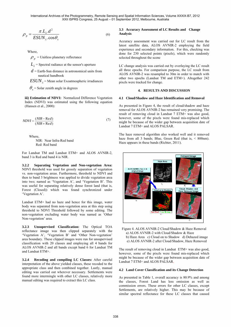
As presented in Figure 4, the result of cloud/shadow and haze removal for ALOS AVNIR-2 has remained very promising. The result of removing cloud in Landsat 7 ETM+ was also good, however, some of the pixels were found mis-replaced which might be because of the wider gap between acquisition date of Landsat 7 ETM+ and ALOS PALSAR. The haze removal algorithm also worked well and it removed haze from all 3 bands; Blue, Green Red (that is, < 800nm). Haze appears in these bands (Richter, 2011).
Figure 4. ALOS AVNIR-2 Cloud/Shadow & Haze Removal a) ALOS AVNIR-2 with Cloud/Shadow & Haze b) Haze Area c) Cloud on to Shadow d) Dehazed image e) ALOS AVNIR-2 after Cloud/Shadow, Haze Removed
The result of removing cloud in Landsat ETM+ was also good, however, some of the pixels were found mis-replaced which might be because of the wider gap between acquisition date of Landsat 7 ETM+ and ALOS PALSAR. 4.2 Land Cover Classification and its Change Detection
As presented in Table 1, overall accuracy is 80.9% and among the classes, Forest Land has less omission as well as commission errors. These errors for other LC classes, except Settlements, are relatively higher. This may be because of similar spectral reflectance for these LC classes that caused
International Archives of the Photogrammetry, Remote Sensing and Spatial Information Sciences, Volume XXXIX-B7, 2012 XXII ISPRS Congress, 25 August – 01 September 2012, Melbourne, Australia
338
misclassification. The LC class “Settlements” was extracted with relatively more manual editing and hence the omission and commission errors for this class are relatively low. Land CoverClass
ForestLand Cropland Grassland Wetlands
Settle-ments
OtherLand
RowTotal
(Pixels)
OmissionError (in %)
Forest Land 94 5 11 2 0 3 115 18.3Cropland 1 28 1 1 0 1 32 12.5Grassland 3 3 29 0 0 2 37 21.6Wetlands 0 2 1 19 0 3 25 24.0Settlements 0 1 0 0 7 0 8 12.5Other Land 0 0 1 3 0 9 13 30.8Column Total(Pixels)
98 39 43 25 7 18 230 -
CommissionError (in %)
4.1 28.2 32.6 24.0 0.0 50.0 - OverallAccuracy = 80.9
Sample Calculation: Omission Error of Forest Land = 21/115 = 18.3% Commission Error of Forest Land = 4 / 98 = 4.1% Overall Accuracy = 186 / 230 = 80.9%
Table 1. Accuracy Assessment of LC Result from ALOS AVNIR-2
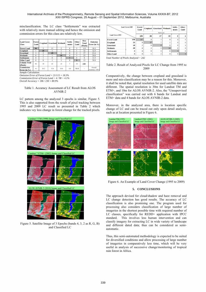
LC pattern among the analyzed 3 epochs is similar, Figure 5. This is also supported from the result of pixel tracking between 1995 and 2009 LC result so presented in Table 2 which indicates vey less change in forest change for the tracked pixels. Figure 5. Satellite Image of 3 Epochs (bands 4, 3, 2 as R, G, B)
and Classified LC
Total Number of Pixels Analyzed = 242
Table 2. Result of Analyzed Pixels for LC Change from 1995 to
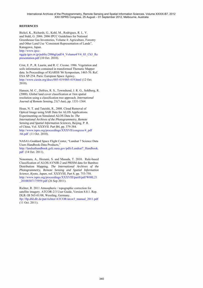
2009 Comparatively, the change between cropland and grassland is more and mis-classification may be a reason for this. Moreover, it shall be noted that, spatial resolution for used satellite data are different. The spatial resolution is 30m for Landsat TM and ETM+, and 10m for ALOS AVNIR-2. Also, the “Unsupervised classification” was carried out with 6 bands for Landsat and ETM+ data and 4 bands for ALOS AVNIR-2 data. Moreover, in the analyzed area, there is location specific change of LC and can be traced out only upon detail analysis, such as at location presented in Figure 6.
Figure 6. An Example of Land Cover Change (1995 to 2009)
5. CONCLUSIONS
The approach devised for cloud/shadow and haze removal and LC change detection has good results. The accuracy of LC classification is also promising one. The program used for processing also considers classification of large number of imageries in the shortest possible time with required number of LC classes, specifically for REDD+ application with IPCC standard. This involves less human intervention and can classify imagery for extracting LC in wide variety of landscape and different dated data; thus can be considered as semi-automatic. Thus, this semi-automated methodology is expected to be suited for diversified conditions and allow processing of large number of imageries in comparatively less time, which will be very useful in analysis of successive change/monitoring of tropical rain forest in Africa.
Landsat 5 TM (1990) Image and Classified LC
Landsat 7 ETM+ (2002) Image and Classified LC
ALOS AVNIR-2 (2010) Image and Classified LC
Landsat TM (1995) Image and Classified LC
Landsat ETM+ (2002) Image and Classified LC
ALOS AVNIR-2 (2009) Image and Classified LC
International Archives of the Photogrammetry, Remote Sensing and Spatial Information Sciences, Volume XXXIX-B7, 2012 XXII ISPRS Congress, 25 August – 01 September 2012, Melbourne, Australia
339
REFERNCES
Bickel, K., Richards, G., Kohl, M., Rodrigues, R. L. V. and Stahl, G. 2006. 2006 IPCC Guidelines for National Greenhouse Gas Inventories, Volume 4: Agriculture, Forestry and Other Land Use “Consistent Representation of Lands”, Kanagawa, Japan. http://www.ipcc-nggip.iges.or.jp/public/2006gl/pdf/4_Volume4/V4_03_Ch3_Representation.pdf (10 Oct. 2010). Crist, E. P., R. Laurin, and R. C. Cicone. 1986. Vegetation and soils information contained in transformed Thematic Mapper data. In Proceedings of IGARSS '86 Symposium, 1465-70. Ref. ESA SP-254. Paris: European Space Agency. http://www.ciesin.org/docs/005-419/005-419.html (12 Oct. 2010). Hansen, M. C., Defries, R. S., Townshend, J. R. G., Sohlberg, R. (2000). Global land cover classification at 1km spatial resolution using a classification tree approach. International Journal of Remote Sensing, 21(7-Jun), pp. 1331-1364. Hoan, N. T. and Tateishi, R., 2008. Cloud Removal of Optical Image using SAR Data for ALOS Applications. Experimenting on Simulated ALOS Data In: The International Archives of the Photogrammetry, Remote Sensing and Spatial Information Sciences, Beijing, P. R. of China, Vol. XXXVII. Part B4, pp. 379-384. http://www.isprs.org/proceedings/XXXVII/congress/4_pdf/66.pdf (11 Oct. 2010). NASA's Goddard Space Flight Center, “Landsat 7 Science Data Users Handbook-Data Products,” http://landsathandbook.gsfc.nasa.gov/pdfs/Landsat7_Handbook.pdf (14 Oct. 2011). Nonomura, A., Hozumi, S. and Masuda, T. 2010. Rule-based Classification of ALOS/AVNIR-2 and PRISM data for Bamboo Distribution Mapping. The International Archives of the Photogrammetry, Remote Sensing and Spatial Information Science, Kyoto, Japan, vol. XXXVIII, Part 8, pp. 753-758. http://www.isprs.org/proceedings/XXXVIII/part8/pdf/W08L21_20100307175959.pdf (26 Sep 2011). Richter, R. 2011 Atmospheric / topographic correction for satellite imagery. ATCOR-2/3 User Guide, Version 8.0.1. Rep. DLR-1B 565-01/08, Wessling, Germany. ftp://ftp.dfd.dlr.de/put/richter/ATCOR/atcor3_manual_2011.pdf (11 Oct. 2011).
International Archives of the Photogrammetry, Remote Sensing and Spatial Information Sciences, Volume XXXIX-B7, 2012 XXII ISPRS Congress, 25 August – 01 September 2012, Melbourne, Australia
340
Recommended


![Shadow Removal by a Lightness-Guided Network with …2 non-shadow regions[17], [18]. Therefore, lightness is a very important cue of shadow regions and following the above two-step](https://img.dokumen.tips/doc/110x75/60ac99797946cc49ff30edb0/shadow-removal-by-a-lightness-guided-network-with-2-non-shadow-regions17-18.jpg)