Selection Of Inventory Control PointsIn Multi-Stage Pull Production Systems
Item Type text; Electronic Dissertation
Authors Krishnan, Shravan K
Publisher The University of Arizona.
Rights Copyright © is held by the author. Digital access to this materialis made possible by the University Libraries, University of Arizona.Further transmission, reproduction or presentation (such aspublic display or performance) of protected items is prohibitedexcept with permission of the author.
Download date 05/06/2018 07:54:41
Link to Item http://hdl.handle.net/10150/193725

SELECTION OF INVENTORY CONTROL POINTS IN MULTI-STAGE
PULL PRODUCTION SYSTEMS
By
SHRAVAN K. KRISHNAN
A Dissertation Submitted to the Faculty of the
DEPARTMENT OF SYSTEMS AND INDUSTRIAL ENGINEERING
In Partial Fulfillment of the Requirements for the Degree of
DOCTOR OF PHILOSOPHY
In the Graduate College
THE UNIVERSITY OF ARIZONA
2 0 0 7

2
THE UNIVERSITY OF ARIZONA
GRADUATE COLLEGE
As members of the Dissertation Committee, we certify that we have read the dissertation
prepared by Shravan K. Krishnan
entitled Selection of Inventory Control Points in Multi-Stage Pull Production Systems
and recommend that it be accepted as fulfilling the dissertation requirement for the
Degree of Doctor of Philosophy.
_______________________________________________________________________ Date: 4/22/07
Ronald G. Askin
_______________________________________________________________________ Date: 4/22/07
Young Jun Son
_______________________________________________________________________ Date: 4/22/07
Jeffrey Goldberg
_______________________________________________________________________ Date: 4/22/07
Srini Raghavan
Final approval and acceptance of this dissertation is contingent upon the candidate‟s
submission of the final copies of the dissertation to the Graduate College.
I hereby certify that I have read this dissertation prepared under my direction and
recommend that it be accepted as fulfilling the dissertation requirement.
________________________________________________ Date: 4/22/07
Dissertation Director: Ronald G. Askin
________________________________________________ Date: 4/22/07
Dissertation Director: Young Jun Son

3
STATEMENT BY AUTHOR
This dissertation has been submitted in partial fulfillment of requirements for an
advanced degree at The University of Arizona and is deposited in the University Library
to be made available to borrowers under rules of the Library.
Brief quotations from this dissertation are allowable without special permission, provided
that accurate acknowledgment of source is made. Requests for permission for extended
quotation from or reproduction of this manuscript in whole or in part may be granted by
the head of the major department or the Dean of the Graduate College when in his or her
judgment the proposed use of the material is in the interests of scholarship. In all other
instances, however, permission must be obtained from the author.
SIGNED: Shravan K. Krishnan

4
ACKNOWLEDGEMENTS
I would like to especially thank my advisor Dr. Ronald Askin, whose guidance and
valuable suggestions helped me to complete my thesis. I would also like to thank my co-
advisor, Dr. Young-Jun Son and my committee members, Dr. Jeffrey Goldberg and Dr.
Srini Raghavan for expressing their willingness to serve on my committee.
I am forever indebted to my parents and my sister for their continuous support and
encouragement.
Finally, I extend my thanks to all my friends in the Systems and Industrial Engineering
Department at the University of Arizona for all their help, especially Karthik Krishna
Vasudevan, who helped me with the Arena models.
5
TABLE OF CONTENTS
ABSTRACT .................................................................................................................................................... 9
CHAPTER 1: INTRODUCTION .................................................................................................................. 11
1.1 BACKGROUND ..................................................................................................................................... 11
1.1.1 A Brief Introduction to Supply Chains ........................................................................................ 13
1.1.2 Production Control Strategies .................................................................................................... 15
1.1.3 Reorder Point (ROP) Models ...................................................................................................... 18
1.1.4 Materials Requirements Planning (MRP) Systems ..................................................................... 19
1.1.5 Kanban Systems .......................................................................................................................... 20
1.1.5.1 Single-card kanban system .................................................................................................................. 21
1.1.5.2 Dual-card kanban system .................................................................................................................... 21
1.1.6 CONWIP Systems ....................................................................................................................... 22
1.1.7 Advantages of Pull Systems over MRP ....................................................................................... 23
1.1.8 Requirements of Pull Systems ..................................................................................................... 24
1.1.9 A Brief Introduction to Queuing Theory ..................................................................................... 25
1.1.9.1 Queuing system ................................................................................................................................... 25
1.1.9.2 Queuing models................................................................................................................................... 25
1.2 MOTIVATION BEHIND OUR RESEARCH ................................................................................................ 27
CHAPTER 2: LITERATURE REVIEW ....................................................................................................... 29
2.1 REORDER POINT RESEARCH ................................................................................................................ 30
2.2 MRP RESEARCH .................................................................................................................................. 37
2.3 KANBAN RESEARCH ............................................................................................................................ 40
2.4 CONWIP RESEARCH ........................................................................................................................... 43
2.5 PROBLEM STATEMENT ......................................................................................................................... 47
CHAPTER 3: SINGLE PRODUCT, DETERMINISTIC MODEL .............................................................. 49
3.1 MODEL 1: CONSTANT CONTAINER SIZE .............................................................................................. 49
3.1.1 Notation ...................................................................................................................................... 50
3.1.2 Model Formulation ..................................................................................................................... 51
3.1.3 Selecting Control Points ............................................................................................................. 53
3.1.4 Choosing Container Size............................................................................................................. 58
3.2 MODEL 2: SECTION DEPENDENT CONTAINER SIZE .............................................................................. 65

6
TABLE OF CONTENTS -- Continued
3.2.1 Solution Procedure ..................................................................................................................... 66
3.3 COMPUTATIONAL RESULTS ................................................................................................................. 71
3.3.1 Experiment Design ...................................................................................................................... 71
3.3.2 Discussion of Results .................................................................................................................. 72
3.3.3 Effect of Value Added Structure on Number of Control Sections ............................................... 79
CHAPTER 4: MULTI-PRODUCT STOCHASTIC MODEL....................................................................... 82
4.1 INTRODUCTION .................................................................................................................................... 82
4.2 ASSUMPTIONS...................................................................................................................................... 83
4.3 MODEL FORMULATION ........................................................................................................................ 84
4.4 DETERMINING THE CONTROL POINTS .................................................................................................. 92
4.5 DETERMINING CONTAINER SIZES ........................................................................................................ 95
4.6 COMPUTATIONAL RESULTS ................................................................................................................. 98
4.6.1 Experiment Design ...................................................................................................................... 98
4.6.2 Discussion of Results ................................................................................................................ 102
4.6.2.1 Effect of factors on cost and control structure ................................................................................... 102
4.6.2.2 Effect of holding cost distribution ..................................................................................................... 105
CHAPTER 5: MODEL VERIFICATION AND VALIDATION ............................................................... 110
5.1 SIMULATION MODEL LOGIC ............................................................................................................... 110
5.1.1 Determining the Number of Kanbans ....................................................................................... 110
5.1.2 Creation of Orders: .................................................................................................................. 111
5.1.3 Simulation Logic ....................................................................................................................... 113
5.1.4 Creation of Entities Corresponding to Containers of Parts and Workstation Logic ................ 114
5.2 MODEL VALIDATION ......................................................................................................................... 118
5.2.1 Methods to Ensure That Both Models Are Equivalent .............................................................. 118
5.2.2 Single Product, Deterministic model ........................................................................................ 119
5.2.3 Single Product Stochastic Model .............................................................................................. 122
5.2.4 Multi Product Stochastic Model ............................................................................................... 125
CHAPTER 6: SUMMARY AND CONCLUSIONS ................................................................................... 129
APPENDIX A: CODE ................................................................................................................................ 131
APPENDIX B: DESIGN TABLE FOR EXPERIMENTS IN SECTION 4.6.2 .......................................... 150
REFERENCES ............................................................................................................................................ 153
7
LIST OF ILLUSTRATIONS
Figure 1.1: The supply chain process ............................................................................... 14
Figure 1.2: Pure pull, CONWIP, and coordinated push systems ...................................... 17
Figure 2.1: System under consideration............................................................................ 48
Figure 3.1: Shortest path representation of Model 1........................................................ 53
Figure 3.2: Shortest path representation for a two-stage control problem ........................ 55
Figure 4.1: Hypothetical structure where stages 4 and 6 are control points ..................... 89
Figure 4.2: Graph showing holding cost at each stage for a 20 stage system with linear
growth. The dotted line indicates a holding cost ratio of 20, while the solid line
indicates a holding cost ratio of 6. .......................................................................... 100
Figure 4.3: Graph showing holding cost at each stage for a 20 stage system with delayed
capitalization. The dotted line indicates a holding cost ratio of 20, while the solid
line indicates a holding cost ratio of 6. ................................................................... 101
Figure 4.4: Graph showing the effect of each factor on system cost. ............................. 104
Figure 4.5: Graph showing the effect of each factor on system control structure. ......... 105
Figure 4.6: Graph showing the combined effect of transportation time and number of
products on the average cost. .................................................................................. 107
Figure 4.7: Graph showing the combined effect of transportation time and number of
products on the ratio of total cost to the number of control points. ........................ 108
Figure 4.8: Graph showing the combined effect of number of stages and number of
products on the system control structure. ............................................................... 109
Figure 5.1: Arrival of orders ........................................................................................... 112
Figure 5.2: Signal code 231 logic ................................................................................... 112
Figure 5.3: Workstations ................................................................................................. 114
Figure 5.4: Logic for signal code: 123 ............................................................................ 116
8
LIST OF TABLES
Table 2.1: Summary of previous relevant research .......................................................... 36
Table 3.1: Comparison of models 1 and 2 ........................................................................ 70
Table 3.2: Comparison of results for model 1 and model 2 .............................................. 74
Table 3.3: Combination of Factors for which model 1 case 1 gives a two-control point 75
Solution ............................................................................................................................. 75
Table 3.4: Combination of Factors for which model 1 case 2 gives a two-control point
solution ...................................................................................................................... 76
Table 3.5: Combination of Factors for which model 2 case 1 gives a two-control point
solution ...................................................................................................................... 77
Table 3.6: Combination of Factors for which model 2 case 2 gives a two-control point
solution ...................................................................................................................... 78
Table 3.7: Summary of Experiments in Section 4.3 ......................................................... 81
Table 4.1: Summary of experiments described in Section 4.6.1 .................................... 103
Table 5.1: Results of experiments described in Section 5.2.2 ........................................ 121
Table 5.2: Results for a single product with Exponential demand. ................................ 124
Table 5.3: Results for a single product with Normal demand. ....................................... 125
Table 5.4: Results of experiments described in Section 5.2.4 ........................................ 127
Table A2.1 Effect of factors on number of control points .............................................. 151
Table A2.2 Effect of factors on system cost ................................................................... 152
9
ABSTRACT
We consider multistage, stochastic production systems using pull control for production
authorization in discrete parts manufacturing. These systems have been widely
implemented in recent years and constitute a significant aspect of lean manufacturing.
Extensive research has appeared on the optimal sizing of buffer inventory levels in such
systems. However the issue of control points, i.e. where in the multistage sequence to
locate the output buffers, has not been addressed for pull systems. Allowable
container/batch sizes, optimal inventory levels, and ability of systems to automatically
adjust to stochastic demand depend on the location of these control points.
We begin by examining a serial production system producing a single part type. Two
models are examined in this regard. In the first, container size is independent of the
control section, while in the second, container sizes are section dependent. Additionally, a
nesting policy is introduced which introduces the additional constraint that the container
size in a section is related to the container size in any other section by a power of two.
Necessary and sufficient conditions are derived for ensuring that a single, end-of-line
accumulation point is optimal. When this is not the case, an algorithm is provided to
determine the optimal control points. Effects of factors such as value added structure,
fixed location cost, setup and material handling cost, kanban collection time, and material
transportation time on the control structure are investigated. Results are extended to

10
determine the optimal container size when lead time at a stage is a concave function of
container size.
The study is then extended to a multi-product case. Queuing aspects are introduced to
account for the interaction between the different part types. The queuing model used is a
modification of the Decomposition/Recomposition model described in Shantikumar and
Buzacott (1981). The models in the chapter do not assume a serial structure any longer.
Additionally, general interarrival and service time distributions are considered. The effect
of number of products, demand arrival distribution, value added structure, and number of
stages on the control structure and system cost is investigated.
Finally, a simulation model is developed in Chapter 5 to verify and validate the
mathematical models described in Chapters 3 and 4.

11
CHAPTER 1: INTRODUCTION
1.1 Background
A manufacturing firm can be thought of as a set of resources and procedures involved in
converting raw material into products and delivering them to the customers. Thus, from
the above definition, among the most important functions of a firm are production and
logistics. Production includes decisions relating to the timing and quantity of production.
The firm also has to decide when to order raw materials from its suppliers. All these
issues come under the realm of inventory control. Single and multi item inventory control
has been widely studied in the past, dating back to 1913 when Harris introduced the EOQ
model. Several distribution strategies too have been examined but they are beyond the
scope of this research. Some of them are discussed in Krishnan (2003) and Krishnan and
Askin (2006), which concentrated on the entire supply chain, encompassing production
and distribution.
A production and distribution system consists of several stages or echelons where each
stage aids in the smooth flow of goods from production to consumption. Beginning with
raw materials, value is added at each stage as the materials are converted into finished
products. The intermediate stages may or may not hold inventory depending on their
function. This type of a system is referred to as a Multi-Echelon System or a Supply
Chain, as it has come to be known. Over the years, the study of multi-echelon systems

12
has generated considerable interest among researchers. The research in this area can find
its roots in the classical work of Clark and Scarf (1960) and Scarf (1960). However much
of the research carried out in this area focuses mainly on simple two-stage systems. In
general a production/distribution system consists of many stages. Viewed from a high
level, a typical system for a large manufacturer may, for instance, consist of six stages,
three for production, and three for distribution. Such would be the case for raw materials,
parts fabrication, and assembly, followed by distribution centers, warehousing, and
retailers. However, within fabrication and assembly, there may be many individual value-
added and transport operations. This research focuses on the control of inventory within a
facility, but the results also provide insights for multi-echelon systems with physically
disbursed stages. In this chapter, we define the relevant terms pertaining to production
control strategies. A brief introduction to supply chain management is also provided. In
Chapter 2, we review some of the relevant research in this area. In Chapter 3, we answer
the important question of where to locate inventory buffers in deterministic, single-
product pull-type serial production systems. Chapter 4 extends these results to a more
general multi-product setting with stochastic demand and interarrival and service times,
and a general structure as opposed to a serial structure. Chapter 5 uses simulation models
to validate the mathematical models described in Chapters 3 and 4.

13
1.1.1 A Brief Introduction to Supply Chains
Various analogous definitions have been proposed for the supply chain. Min and Zhou
(2002) define the supply chain as:
“an integrated system which synchronizes a series of inter-related business processes in
order to: (1) acquire raw materials and parts; (2) transform these raw materials and parts
into finished products; (3) add value to these products; (4) distribute and promote these
products to either retailers or customers; (5) facilitate information exchange among
various business entities (e.g. suppliers, manufacturers, distributors, third-party logistics
providers, and retailers).”
Lee and Billington (1995) have a similar definition:
“A supply chain is a network of facilities that procure raw materials, transform them
into intermediate goods and then final products, and deliver the products to customers
through a distribution system. “
Swaminathan et al. (1996) define the supply chain to be:
“a network of autonomous or semi-autonomous business entities collectively
responsible for procurement, manufacturing, and distribution activities associated
with one or more families of related products. “
14
In short, a supply chain can be said to consist of “all the stages involved, directly or
indirectly, in fulfilling a customer request.” (Chopra and Meindl (2001)).
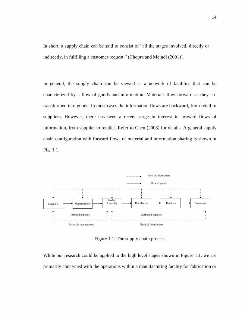
In general, the supply chain can be viewed as a network of facilities that can be
characterized by a flow of goods and information. Materials flow forward as they are
transformed into goods. In most cases the information flows are backward, from retail to
suppliers. However, there has been a recent surge in interest in forward flows of
information, from supplier to retailer. Refer to Chen (2003) for details. A general supply
chain configuration with forward flows of material and information sharing is shown in
Fig. 1.1.
Suppliers
Customers
Retailers
Distributors
Manufacturers
Materials management
Outbound logistics
Physical Distribution
Inbound logistics
Flow of goods
Flow of information
Product
Assembly
Figure 1.1: The supply chain process
While our research could be applied to the high level stages shown in Figure 1.1, we are
primarily concerned with the operations within a manufacturing facility for fabrication or

15
assembly. In the following sections we provide an overview of the systems and control
elements within these environments.
1.1.2 Production Control Strategies
Single stage production control models frequently use Reorder Point (ROP) inventory
models. These models are based on the EOQ model and will be discussed briefly in the
following section. Production and inventory control strategies used in multi-echelon
systems can be divided into three basic categories depending on the protocol for
authorizing production or distribution and the timing of process execution. A push system
is one in which processes are executed based on a centrally coordinated plan, often
external to the local process and based on demand forecast. Production authorization is
based on upstream conditions or centralized control and the approach is to actually plan
production levels. Push systems can be of two types: coordinated push systems and open
systems. A coordinated push system is one in which an external coordinator uses
forecasts to coordinate production and distribution decisions for all stages. An open
system reacts to the arrival of orders. Once released, orders are executed as soon as
resources are available. A Materials Requirement Planning (MRP) system is a commonly
used push system. A pull system is one in which processes are executed in response to
status changes in the downstream process. In a pull-based system, production is demand
driven so that it is coordinated with actual customer demand rather than a forecast. In
pull systems, the level of inventory in the system is controlled. Production authorization

16
is determined by downstream conditions. Commonly used Kanban pull systems control
the level of each part in between inventory storage locations. CONWIP (Constant Work-
In-Process) is a hybrid system. Orders are released as in a pull system but thereafter,
follow a push protocol generally. The three systems are shown Fig. 1.2. The ROP model
and Kanban, MRP and CONWIP systems will be discussed in the following sections.

17
`
Pull system
Demand forecasts
(possibly)
Manufacturing stage
Flow of material
Flow of information
CONWIP system
Information
Material
Base stock system
Orders
Demand
information
Coordinated Push system
Coordinator
Production/ distribution
decisions
Demand
information
Buffer
Figure 1.2: Pure pull, CONWIP, and coordinated push systems
18
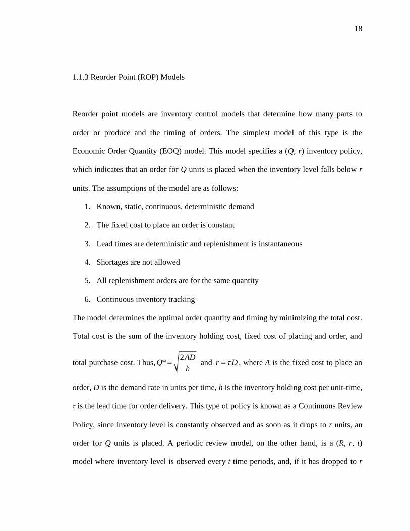
1.1.3 Reorder Point (ROP) Models
Reorder point models are inventory control models that determine how many parts to
order or produce and the timing of orders. The simplest model of this type is the
Economic Order Quantity (EOQ) model. This model specifies a (Q, r) inventory policy,
which indicates that an order for Q units is placed when the inventory level falls below r
units. The assumptions of the model are as follows:
1. Known, static, continuous, deterministic demand
2. The fixed cost to place an order is constant
3. Lead times are deterministic and replenishment is instantaneous
4. Shortages are not allowed
5. All replenishment orders are for the same quantity
6. Continuous inventory tracking
The model determines the optimal order quantity and timing by minimizing the total cost.
Total cost is the sum of the inventory holding cost, fixed cost of placing and order, and
total purchase cost. Thus,2
*AD
Qh
and r D , where A is the fixed cost to place an
order, D is the demand rate in units per time, h is the inventory holding cost per unit-time,
τ is the lead time for order delivery. This type of policy is known as a Continuous Review
Policy, since inventory level is constantly observed and as soon as it drops to r units, an
order for Q units is placed. A periodic review model, on the other hand, is a (R, r, t)
model where inventory level is observed every t time periods, and, if it has dropped to r
19
units, an order is placed to bring the inventory position to R. EOQ-type models are used
for bulk materials and make-to-stock environments. More sophisticated continuous and
periodic review models are discussed in Askin and Goldberg [2002] and other production
planning textbooks. Section 2.1 contains a review of these models applied to multi-stage
production systems.
1.1.4 Materials Requirements Planning (MRP) Systems
An MRP system, as mentioned earlier, is a type of push system. In an MRP system,
orders for all the component parts that go into a product are timed so that they coincide
with the production schedule of that product. This is the basis for a dependent demand
relationship. In the best case, there is very little safety stock carried, since production is
carried out only when parts are required. This system is designed for low to intermediate
volume production with moderate to high product variety.
The various data requirements of an MRP system include:
1. Item master data for each part: this contains data pertaining to the annual
demand, order quantity, cost, and scrap rate for each product. In addition, for
internally created products, there is a link to engineering drawings and process
plans.
2. Inventory status records for each item: contains data relating to on-hand
inventory for each item.
20
3. Lead times: this helps in determining when to place an order for each item.
Lead times are assumed to be deterministic.
4. Bill of materials: bill of materials is a listing of all the materials and
components required to make each item produced in the factory. This includes
all manufactured parts, subassemblies and end items.
5. Master Production Schedule (MPS): this shows planned production quantities
for each end item in each period of the planning horizon.
MRP systems suffer from several inherent problems, some of which are discussed in
Section 2.2.
1.1.5 Kanban Systems
A kanban system, as mentioned earlier, is a type of pull system. In this system,
production authorization to produce a part at a workstation comes from the downstream
stage. This production authorization comes in the form of a kanban card (virtual or
physical). Each kanban card authorizes the production of one container of parts. Each
workstation is in charge of keeping a full container of parts in its output buffer for each
kanban allocated to it. Thus, the maximum number of parts (units) at any given time at a
workstation is given by the product of the number of kanbans and the number of parts
authorized by each kanban (usually, container size). There are two important types of
kanban systems, single-card kanban systems and dual-card kanban systems. These
systems are briefly discussed in the next two sections.
21
1.1.5.1 Single-card kanban system: This system is preferred when workstations are close
to each other. In this system, there is a single set of kanbans, known as production
ordering kanbans (POK). When an operator at work station i produces a container of
parts (after receiving the authorization to produce it), he puts the kanban associated with
it into the container and sends the container to the output buffer. When the operator at
workstation i+1 requires the parts, he withdraws the container from the output buffer of
workstation i and places the kanban into a collection box. Kanbans are regularly collected
from the collection box and arranged in a schedule board. When the operator at
workstation i becomes free, he checks the schedule board for kanbans.
1.1.5.2 Dual-card kanban system: A dual kanban system is used when distances between
workstations are large. In addition to production ordering kanbans (POKs), this system
uses withdrawal ordering kanbans (WOKs). The system has two loops, the first loop is
the same as in Section 1.1.4.1 – the POKs move from the input buffer to the output buffer
to the collection box to the schedule board. The WOKs loop from the input buffer of
stage i+1 to their own collection box at i+1 to the output buffer of stage i, back to the
input buffer of stage i+1. The material handler at stage i+1 checks the collection box
frequently. If there are any WOKs present, the material handler moves to the output
buffer at stage i to collect containers of parts authorized by the kanban. It removes the
POKs from the container and places them in the collection bin and places the WOKs into
the container instead. Thus, production and transportation are both controlled by this
22
method. Workstations have an input buffer for their raw material and an output buffer for
their finished product.
A review of literature related to kanban systems is carried out in Section 2.3.
1.1.6 CONWIP Systems
CONWIP (Constant Work-In-Process) could be thought of as a hybrid system. Orders are
released as in a pull system but thereafter, follow a push protocol generally. Like the
kanban system, a CONWIP system maintains a constant WIP in the system. However,
unlike a kanban system that has a WIP cap at each stage and for each part, a CONWIP
system maintains a WIP cap at the system level, that is, there is a total of N parts in the
system at all times (irrespective of the part type). A backlog list is maintained, which
contains a list of parts to be manufactured. As soon as one batch completes processing,
the next batch on the backlog list for which all raw materials are available is sent for
processing. Whereas in a kanban system the internal distribution of jobs among part types
and workstations is controlled, only total inventory is controlled in a CONWIP system.
This makes it easier to manage the system. Especially when there are a large number of
parts to produce, a CONWIP system is easier to manage than a kanban system. On the
other hand, a CONWIP system requires more storage space, since, all N jobs need to be
potentially accommodated at a workstation. Some of the methods for determining job

23
ordering in the backlog list are discussed in Section 2.4. Variants of CONWIP exist such
as only controlling the inventory upstream of a bottleneck workstation.
1.1.7 Advantages of Pull Systems over MRP
A pull system has several advantages over an MRP system. Some of these advantages are
briefly discussed in this Section.
1. Efficiency - pull systems attain the same throughput as push systems with less
average WIP.
2. Ease of control – it is easier to set WIP levels than to set release rates (throughput)
3. Robustness - pull systems are less affected by data errors and random events than
push systems. They are also self adjusting to minor variations.
4. Low Information System Requirement – due to the manner in which they are
designed, pull systems have lower information requirements than push systems.
5. Support for improving quality – since WIP levels are low in pull systems, they
not only require quality in order to prevent disruptions, but also promote it by
shortening queues and quickening defect detection.
(Source: Askin & Goldberg (2002) and Hopp & Spearman (1996))
24
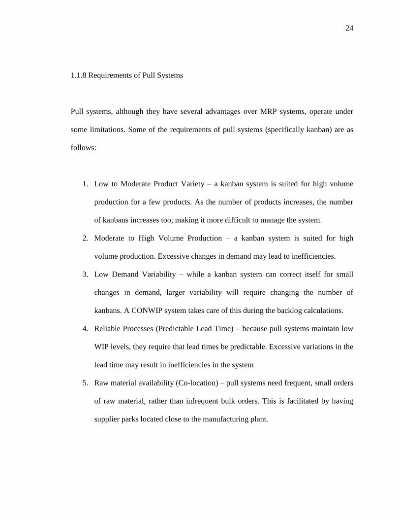
1.1.8 Requirements of Pull Systems
Pull systems, although they have several advantages over MRP systems, operate under
some limitations. Some of the requirements of pull systems (specifically kanban) are as
follows:
1. Low to Moderate Product Variety – a kanban system is suited for high volume
production for a few products. As the number of products increases, the number
of kanbans increases too, making it more difficult to manage the system.
2. Moderate to High Volume Production – a kanban system is suited for high
volume production. Excessive changes in demand may lead to inefficiencies.
3. Low Demand Variability – while a kanban system can correct itself for small
changes in demand, larger variability will require changing the number of
kanbans. A CONWIP system takes care of this during the backlog calculations.
4. Reliable Processes (Predictable Lead Time) – because pull systems maintain low
WIP levels, they require that lead times be predictable. Excessive variations in the
lead time may result in inefficiencies in the system
5. Raw material availability (Co-location) – pull systems need frequent, small orders
of raw material, rather than infrequent bulk orders. This is facilitated by having
supplier parks located close to the manufacturing plant.

25
6. High Quality Requirements (lower setup times, higher machine availability, lower
defect percentage) – as a result of low WIP levels maintained, pull systems
demand high quality.
7. Small setup times – since pull systems react instead of planning, a pull system
requires low setup times to rapid response and low inventory levels.
1.1.9 A Brief Introduction to Queuing Theory
Queuing theory is extensively used to analyze manufacturing systems and supply chains.
In this Section, we provide a brief introduction to some of the concepts.
1.1.9.1 Queuing system: A queuing system protocol provides the basis for how items
enter and leave the queue. Some examples of queuing system protocols are:
FIFO (First In First Out) also known as FCFS (First Come First Serve) – parts are
processed in the order in which they arrive.
LIFO (Last In First Out) also known as LCFS (Last Come First Serve) – similar
to a stack where the last part to arrive is served first.
Priority Queue where certain parts have higher processing priority than others.
Random order
1.1.9.2 Queuing models: Queuing models are used to model systems. They describe the
following characteristics of the queuing systems:

26
Part arrival process: this describes the arrival distribution, whether parts arrive
individually or in batches.
Service times
Server capacity: the number of available servers.
Queue capacity: the number of available spaces in the queue.
Queue discipline: as explained in section 1.1.9.1.
Kendall introduced a shorthand notation to characterize a range of these queuing models.
It is a three-part code a/b/c. The first letter specifies the interarrival time distribution, the
second the service time distribution, while the third letter indicates the number of servers.
For example, a (b) can be „M‟, which indicates an exponential interarrival (service time)
distribution, „D‟, which indicates a deterministic times or „G‟, which indicates a general
distribution. The parameter c can be any number equal to or greater than 1. In case the
queue has a finite capacity, a fourth letter is added to the notation to indicate queue
capacity, for example, M/M/1/5, which means that interarrival and service times are
exponential, there is a single server, and the queue has room only for five parts.
Some of the performance measures include
1. The distribution of number of customers in the system
2. The distribution of service times of customers in the system and in queue (amount
of work in the system).
3. The distribution of the busy period of the server
27
An extensive theory survey of queuing theory in manufacturing systems has been carried
out by Govil and Fu (1999). Little‟s Law (1961) relates the queue length to service rate
and waiting time for systems in steady state.
1.2 Motivation Behind Our Research
Extensive research has been carried out on pull control based production systems as one
aspect of lean manufacturing. In such systems, each inventory storage buffer is
designated with a desired level of inventory for each part type. This level is typically
defined as a desired number of containers with each container holding a designated
quantity of the product. This quantity is referred to as the container size. Following the
procedure popularized by the successful Toyota Production System, “kanbans” or cards
are used to authorize production. Each kanban corresponds to one container. Kanbans
are kept in the output buffer attached to a full container of parts. When the first part from
that container is required by the succeeding work area, the container is removed from
storage and the kanban is recirculated to the production station to authorize replenishment
of those items. The system automatically paces and prioritizes orders within workstations
based on downstream consumption. This makes the system easy to implement and self-
adjusting. If the proper level of kanbans is selected, and the replenishment and demand
processes are highly predictable and deterministic, then the system can be operated such
that a completed container of parts reenters the output buffer just in time for its need at

28
the downstream workstation. Hence, such systems are often considered part of the JIT
(Just-in-Time) production control philosophy.
Most of the previous pull-system research focused on determining the number of
kanbans, with lesser emphasis placed on container sizes and product sequence in a just-
in-time (JIT) shop. However, in a multistage system, it is not necessary to include an
output buffer at each stage. Within control sections (the area or sequence of workstations
between buffers), a push philosophy can be incorporated. Once production is authorized
by the removal of a container from the control sections‟ output buffer, a replenishment
order is released to the first workstation in the control section. These orders then have
authorization to flow through each stage of the control section until again reaching the
output buffer, i.e. they are pushed through without waiting for a customer request. The
issue of where to locate control points, although important, has not been effectively
addressed in the past. In our study, we attempt to find a set of production stages in a JIT
system that will act as inventory control points. These control points are the only stages
that store inventory. In addition, we determine the number of kanbans and container
sizes that should be used in specific conditions. Chapter 3 deals with a single product
deterministic case. In Chapter 4, this is extended to a multi-product stochastic case.
29
CHAPTER 2: LITERATURE REVIEW
During the last few years there has been considerable interest in studying problems
pertaining to inventory management in multistage production/distribution systems.
Multistage problems are complex and the same solution procedures used for single-stage
systems are not appropriate to be used to solve them. According to Clark and Scarf
(1960), in studying single-stage systems, the main assumption that was made was that
when the installation requests a shipment of stock, this shipment is delivered in a fixed or
random length of time, but the time lag is independent of the order placed. However there
are several situations where this assumption may not be valid and hence the need to study
multi-echelon systems arose. It has also been shown by Muckstadt and Thomas (1980)
that specialized multi-level methods may reduce the total costs substantially over general
methods for single stage systems. In this Chapter we first review research in multistage
systems using general reorder point policies. Next we will discuss research on MRP,
Kanban, and CONWIP systems.

30
2.1 Reorder Point Research
One of the first studies in this area is the seminal work of Clark and Scarf (1960), who
analyze a serial system under a periodic review policy and uncertain end-item demand.
They show that for such a system, the problem can be decomposed and the optimal policy
at each echelon can be computed separately to get approximate solutions that provide
upper and lower bounds on the actual costs. Each echelon in this case is linked by a
penalty function, which represents the cost of failing to fulfill a downstream stage‟s
order. The late eighties and the early nineties saw a surge in papers related to these areas.
For a comprehensive review of the research in this area, the reader is referred to Axsater
(1993). In this Section we summarize some of the recent research in this area and classify
the models based on certain characteristics, such as, whether a periodic review or a
continuous review policy is used, whether end-item demand is stochastic or deterministic,
and whether a finite or infinite horizon is used. In addition, some of the recent models for
solving this problem will be discussed.
We begin by looking at a serial system with N stages. For this system, it has been shown
that the base quantities at different stages follow the integer ratio property, i.e., the base
quantity at a stage is an integer multiple of the base quantity at the next stage (assuming
that demand occurs at the last stage). Clark and Scarf (1960, 1962) examine the problem
of determining optimal purchasing quantities using base-stock policies in a finite-horizon,
by decomposing the problem and solving for the optimal quantity at ever stage. They
31
show that in the absence of economies of scale, these policies are optimal. A base stock
system is similar to a pull system. It can be defined as an (S, S) order up to policy where
each stage acts in unison to replace consumed stock. An (s, S) inventory system is one
where whenever inventory level falls below s, an order is placed to raise the level up to S.
In (S, S), once a retailer sells one unit of product, he places an order with the previous
stage to replenish its stock. Thus the stock level is kept constant. The model makes the
following assumptions:
The cost of purchasing and shipping an item from any stage to the next will be
linear, without any setup cost. The only exception to this is at the first stage.
At the last stage, a linear holding cost and shortage cost will be operative.
Excess demand is backlogged.
Federgruen and Zipkin (1984) extend this model to an infinite horizon and prove that the
results of Clark and Scarf (1960) are applicable for this case. Roundy (1986) and
Maxwell and Muckstadt (1985) devise simple policies that are within 2% of the optimal
solution. This results from restricting order intervals to powers-of-two times some base
time period . Thus, if nT is the order interval for product n, then: 2 nk
nT where
1 2 and nk is some integer. It is assumed that Zero-Inventory Policy holds, i.e., an
order is placed for a product only when its inventory drops to zero. Dong and Lee (2003)
prove that the results of Clark and Scarf (1960) can be extended to a time-correlated
demand process using Martingale Model of Forecast Evolution (MMFE), a forecasting
technique that takes into account past demand and other factors affecting demand.
32
A substantial amount of research has gone into determining the size and location of safety
stock inventory under various production control strategies. Inderfuth (1991) provides a
technique for determining safety stock distribution in serial and divergent
production/distribution systems operating under base stock policies. The paper assumes
100% reliable workstations. Inderfuth and Minner (1997) look at divergent systems with
normally distributed demands where each stage follows a base stock policy. Inderfuth
(1994) contains a review of relevant research in this area. The paper is a survey on
concepts and specific approaches for determining safety stocks in divergent inventory
systems as a measure of protection against risk. Graves and Willems (2000) develop an
approach to optimize the inventory in a supply chain. Each stage in the supply chain is
modeled as a network. They make the following assumptions:
Each stage in the supply chain operates under a periodic-review, base-stock
policy.
Production lead times are assumed to be known and deterministic.
Demand occurs at stages without successors and is bounded.
Each demand node promises a guaranteed service time by which it will satisfy
customer demand.
For a serial system based with the above assumptions and without any capacity
constraints, Simpson (1958) provides a technique to optimize the inventory. van Houtum
et al (1996) also review relevant research in the theoretical and numerical analysis of
stochastic multistage systems where a periodic review base-stock policy is used.
33
Magnanti et al (2005) show that adding a set off redundant constraints and iteratively
refining the approximation speeds up the time required on a commercial solver to solve
moderately sized safety stock placement problems in acyclic supply chain networks.
Minner (2001) analyzes the problem of safety stock placement in reverse supply chains
with the integration of internal and external product return and reuse.
For assembly systems where two components are assembled into one so that each stage
has a unique successor, Crowston, Wagner, and Williams (1973) state that in an optimal
solution, an Integer-Ratio property holds, i.e., the batch size at a stage is an integer
multiple of the batch sizes at its downstream stages. It was shown by Szendrovits (1981)
and Williams (1982) that their results were highly dependent on the assumptions they
used. For example, Williams (1982) shows that when the assumption that production
occurs at a constant rate at a stage is ignored, the proposition no longer holds. Schmidt
and Nahmias (1985) use the decomposition technique of Clark and Scarf to characterize
the optimal policy for an assembly system where two components are assembled into
one. Rosling (1989) states that under appropriate conditions, a general assembly system is
equivalent to a serial system and so the result of Clark and Scarf holds. Chen (2000)
extends these results to an assembly system with batch-ordering. Cachon (1995), Graves
(1996), Chen and Zheng (1997), Tarim and Miguel (2004) all study distribution systems.
DeBodt and Graves (1985) design approximate echelon stock policies for a serial system
with setup costs under a continuous review policy with batch ordering. Echelon stock for
34
a component is defined as the inventory of that component plus all the inventory of
downstream items that use that component. Installation stock, on the other hand, is
inventory of the component without considering downstream inventories. Echelon stock
policies use echelon stock information to make decisions. The end customer demand is
stationary and stochastic and each stage has a deterministic lead time. They assume
nested policies, where, whenever one stage reorders, all downstream stages also reorder.
Chen and Zheng (1994) provide an exact cost evaluation procedure for such systems.
Axsater and Rosling (1993) prove that echelon stock policies are superior to installation
stock policies for serial and assembly systems. Axsater (1997) provide an exact cost
evaluation technique for a two-stage system with one warehouse and N retailers, where
all facilities use a continuous review echelon-stock policy with different reorder points
and batch quantities. An echelon stock policy requires centralized demand information.
Chen and Zheng (1998) study serial systems with compound Poisson demand and batch-
ordering and provide a near-optimal solution. Chen (1998) determines the relative cost
difference between the two policies for a serial system. This cost difference can be
thought of as the value of centralized demand information. Mitra and Chatterjee (2003)
extend the results of DeBodt and Graves (1985) to fast moving items.
Information sharing and coordination are two topics that have been extensively studied in
multi stage systems, but more so from a supply chain perspective. Papers by Lee et al.
(1997a & b), Gavirneni et al. (1999), Chen et al. (1998, 2000a & b) and more recently,

35
Krishnan and Askin (2006) have studied the effect of information sharing and
coordination between supply chain partners on the system performance.
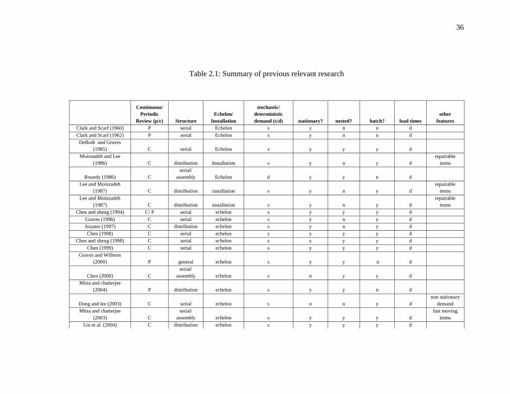
Table 2.1 below summarizes some of the papers on production planning in multi-echelon
systems.
36
Table 2.1: Summary of previous relevant research
Continuous/
Periodic
Review (p/c) Structure
Echelon/
Installation
stochastic/
deterministic
demand (s/d) stationary? nested? batch? lead times
other
features
Clark and Scarf (1960) P serial Echelon s y n n d
Clark and Scarf (1962) P serial Echelon s y n n d
DeBodt and Graves
(1985) C serial Echelon s y y y d
Moinzadeh and Lee
(1986) C distribution Installation s y n y d
repairable
items
Roundy (1986) C
serial/
assembly Echelon d y y n d
Lee and Moinzadeh
(1987) C distribution installation s y n y d
repairable
items
Lee and Moinzadeh
(1987) C distribution installation s y n y d
repairable
items
Chen and zheng (1994) C/ P serial echelon s y y y d
Graves (1996) C serial echelon s y n y d
Axsater (1997) C distribution echelon s y n y d
Chen (1998) C serial echelon s y y y d
Chen and zheng (1998) C serial echelon s y y y d
Chen (1999) C serial echelon s y y y d
Graves and Willems
(2000) P general echelon s y y n d
Chen (2000) C
serial/
assembly echelon s n y y d
Mitra and chatterjee
(2004) P distribution echelon s y y n d
Dong and lee (2003) C serial echelon s n n y d
non stationary
demand
Mitra and chatterjee
(2003) C
serial/
assembly echelon s y y y d
fast moving
items
Liu et al. (2004) C distribution echelon s y y y d

37
2.2 MRP Research
A Materials Requirement Planning (MRP) system is a type of push system where
production authorization is based on a production plan. In contrast, in pull systems,
production authorization depends on realized demand. A significant amount of the early
research in this area focused on lot sizing decisions associated with MRP. Several lot
sizing models have been developed in the last couple of decades. The simplest lot sizing
model is the Economic Order Quantity (EOQ) model, which dates back to 1913. Another
model used for lot sizing in MRP systems is the Wagner-Whitin (WW) model (Wagner
and Whitin, 1958). This model was originally developed for a multi-period single-stage
model under a periodic review policy with known time-varying demands. They assume
linear holding costs and fixed order costs and that shortages are not permitted. For this
cost structure they determine that in an optimal policy production is carried out only in
periods with positive starting inventory. Dynamic programming can be used to determine
optimal production quantities. However, the WW model has not been frequently used in
MRP systems. This is due to the fact that the model has an inherent property that causes
nervousness in the system, i.e., alterations or changes in schedules for later periods may
cause changes in lot sizes during the early periods. Another model that is used is a
heuristic developed by Silver and Meal (1973). It involves computing the cost of holding
and setup per period as a function of the number of periods in the current order horizon
and using it to calculate the order quantity. Lot-for-lot (LFL) is a strategy where order
quantities are equal to the requirements, offset by the lead time. Another popular
38
technique known as Periodic Order Quantity (POQ) calculates the optimal order interval,
T as a ratio of the EOQ to the demand rate and assigns the first T periods‟ demands to the
first period and so on. The Least Period Cost (LPC) method determines the first local
minimum cost per unit time and sets the first lot size quantity and proceeds to the next lot
size. Other lot sizing techniques have been developed by Veral and LaForge (1985),
Blackburn and Millen (1982), Afentakis et al. (1983), Afentakis and Gavish (1983),
Afentakis (1987) etc. Texts and articles such as Askin and Goldberg (2002) and Baker
(1993) contain a thorough description of these models.
Molinder and Olhager (1998) study the effect of different lot sizing techniques on
cumulative lead times. Here, cumulative lead time is the total lead time for each bill of
material path below the item. Buzacott and Shantikumar (1994) study the influence of
accuracy of forecasts, processing time variability, and degree of congestion, along with
inventory and shortage costs on system lead time and safety stock, in order to determine
whether safety stock or safety time is more useful. They conclude that safety stock is
more robust than safety time, except when it is possible to make accurate forecasts over
the lead time. Other studies on MRP system performance include, Whybark and Williams
(1976), Grasso and Taylor (1984), and Ritzman and King (1991).
MRP uses fixed lead times for planning. However in reality, lead times are variable. This
lead time variability may result in inefficiency in planning. Melnyk and Piper (1985)
suggest the following two options to overcome these problems:
39
Track lead time error, i.e., the difference between planned lead times and
observed lead times, and update planned lead times appropriately.
Minimize the effect of lead time error by constructing planned lead times that
provide an appropriate probability that actual lead times will not exceed the
planned lead times.
Several comparative studies have been carried out comparing the performance of MRP
with Kanban, CONWIP, and Reorder Point Policies. Benton and Shin (1998) classify
existing MRP/ JIT comparison literature. Recently, Krishnamurthy et al. (2004) have
shown using simulation experiments that Kanban may result in significant inefficiencies
in a manufacturing setting where a fabrication cell supplies different products to several
assembly cells. It is assumed that the assembly cells fix their assembly schedules in
advance and share this information with the supplier cells. Axsater and Rosling (1994)
have shown that MRP outperforms installation stock (Q, r), Kanban, and order-up-to-R
policies for a general acyclic inventory system. More of the literature on these
comparative studies will be discussed in the following two sections.
The MRP system suffers from several drawbacks, both due to the assumptions that it
makes and due to its basic structure. One of the most important assumptions that MRP
makes is that there is always sufficient capacity to meet production demands, which is
unrealistic. As mentioned earlier, MRP uses fixed lead times for planning. Also, MRP
plans for periods, not continuous time, thus requiring inventory to be pre-staged. Our

40
research focuses on pull systems, such as CONWIP and Kanban, which will be discussed
in the following two Sections.
2.3 Kanban Research
One of the earliest descriptions of the single kanban system was given by Monden (1983)
as being used in the Toyota Production System for serial systems with closely located
sequential stages. An overview of various extensions and refinements is given in Askin
and Goldberg (2002). A thorough review of the research in Kanban systems is available
in Huang and Kusiak (1996).
Most research into Kanban systems has emphasized the choice of the number of kanbans
to use in such systems. Monden (1983) suggests the following model:
(1 )i ii
i
D lk
n
where ki is the number of kanbans for part type i, i is the total lead time, Di is the
demand rate and ni is the container size. l is a safety factor, introduced to counter
variability. The container size associated with each part type can be determined using the
EOQ expression:
2 i ii
i
a Dn
h ,

41
where ai is the setup cost and hi is the holding cost per unit for product i. Schonberger
and Schniederjans (1984) suggest that the EOQ model may be inappropriate for the JIT
manufacturing environment. They claim that reductions in setup time and a proper value
of holding costs will result in an optimal batch size of one. The value of setup time
reduction is discussed in papers by Spence and Porteus (1987) and Hahn et al. (1988).
Davis and Stubitz (1987) determined the number of kanbans at each station using
simulation and response surface techniques. Philipoom et al. (1987) showed
experimentally that the lead time demand distribution constitutes a major determinant of
the number of kanbans needed. For modeling a kanban system with a fixed parameter
specification or to determine the number of kanbans needed, stochastic analytical models
with discrete time periods (Deleersnyder et al. 1989) and continuous time (Mitra and
Mitrani 1990, Wang and Wang 1990, Askin et al. 1993) have also been presented.
Deleersnyder et al. (1989) use a discrete time markov chain to determine the number of
kanbans. They take machine reliability, demand variability, and safety stocks into
account. Askin et. al (1993) develop a mathematical programming model to determine
the number of kanbans under time dependent backorder costs and occurrence based
shortage costs by minimizing total system costs. Philipoom et al. (1996) present a
solution procedure known as JACKS (JIT Algorithm for Containers, Kanbans and
Sequence) that provides an integrated approach to simultaneously determine container
sizes, number of kanbans, and product sequence.

42
Karmarkar and Kekre (1989) model two-stage, single and dual card kanbans as a
Continuous Time Markov Chain in order to study the effect of container size and number
of kanbans on the expected inventory holding costs and shortage costs. They conclude
that when the number of kanbans was constant, the total inventory cost was a convex
function of the container size. In another experiment, the optimal container size was seen
to be inversely proportional to the number of kanbans. Berkeley (1996) studies the effect
of container size on average inventory and customer service levels in a two-card kanban
system processing multiple part types. The study concludes that, as expected, smaller
container sizes resulted in smaller average inventories. However, they do not necessarily
lead to lower service levels. Some other studies that consider the effect of container sizes
on the system performance include, Gupta and Gupta (1989a & b) and Lee (1987).
Another area of research in Kanban system compares the performance of kanban systems
with other systems, notably MRP systems. Rees et al. (1989) compared an MRP lot-for-
lot system and a Kanban system in an ill-structured production environment and
concluded that the MRP lot-for-lot system is comparatively more cost effective since it
carries less inventory. Sarker and Fitzsimmons (1989) concluded that an MRP lot-for-lot
handles lumpy demand better than a Kanban system, although difficulties may be caused
by stochastic processing times.

43
2.4 CONWIP Research
The Constant Work In Process (CONWIP) system was proposed by Spearmann et al.
(1990) as an alternative to the Kanban production system. Spearmann and Zazanis (1992)
present the following conjectures about pull systems:
There is less congestion in pull systems
1. Pull systems are inherently easier to control than push systems.
2. The benefits of a pull environment owe more to the fact that WIP is bounded than
to the practice of “pulling” everywhere.
The CONWIP system imposes a WIP cap on the entire system, rather than on individual
workstations, as in a Kanban system. In fact, CONWIP could be thought of as a hybrid
pull-push system, where parts enter the system according to a pull philosophy, but within
the system, a push policy is used. A backlog list is used to determine the order in which
jobs are processed.
Initial studies into the CONWIP system were comparisons of this system with MRP and
Kanban systems. Spearmann et al (1990) provide a brief comparison of CONWIP with
MRP and kanban systems and conclude that a CONWIP system is more effective than the
other two systems. Buzacott and Shantikumar (1991) show that if the value added at each
stage in the workstation is negligible, then CONWIP systems exhibit superior
performance to Kanban and MRP systems with respect to maximizing customer service,
subject to WIP constraint. Spearmann and Zazanis (1992) compare Kanban and
44
CONWIP and conclude that CONWIP produces higher mean throughput. Spearmann and
Zazanis (1992) and Hopp and Spearmann (1996) suggest that CONWIP systems possess
the following advantages over MRP systems:
1. Pull systems are easier to control than push systems. This is because pull systems
control WIP and observe throughput, whereas push systems control throughput
and observe WIP. It is easier to control the total number of parts currently in the
system than to control the production rate.
2. For the same throughput, push systems will have more WIP on an average than
CONWIP systems. A corollary of this is that for the same throughput, push
systems will have longer average cycle times than an equivalent CONWIP
system.
3. A CONWIP system is more robust to errors and breakdowns than a pure push
system.
Muckstadt and Tayur (1995a, b) show that the CONWIP system has less variable
throughput and lower inventory than a Kanban system. Golany et al. (1999) investigate
CONWIP based Shop Floor Control (SFC) where products are grouped into families
(Group Technology (GT) design). The main reason for GT grouping is to cluster different
parts having almost identical routings into families. This creates a flowshop-like
environment within each family of parts. The authors propose that within each cell, parts
be scheduled as a CONWIP system. They attempt to simultaneously answer two
questions: 1. what is the best WIP level? and 2. how to arrange the backlog level for a
given system? They formulate a deterministic mathematical programming formulation to

45
describe the scenario and solve it using simulated annealing. They compare two systems.
In the first, a multi-loop CONWIP system, containers are restricted to stay in given cells,
while in the second, a single-loop CONWIP system, containers can circulate anywhere in
the system. Based on their results they find the latter system to be superior. A recent
study by Yang (2000) uses simulation based techniques to compare Kanban and
CONWIP systems. He concludes that CONWIP outperforms Kanban in most cases,
consistently producing the smallest mean customer wait and total WIP. Recent textbooks
by Hopp and Spearmann (1996) and Askin and Goldberg (2002) contain in depth
comparisons of the two systems with each other and with MRP systems.
Recent research has focused on determining system parameters, such as, how to order
jobs in a backlog list and how many containers to use. CONWIP is a type of closed
queueing nework. In these networks, the number of parts in the system never changes. In
essence, if a part leaves the system, it is immediately replaced with another part, which
keeps the WIP constant. This results in a negative correlation between the parts at each
stage. A product form expression for such a system may not be computationally very
effective, instead, a technique known as Mean Value Analysis (MVA) (Reiser and
Lavenberg 1980, Suri and Hildebrant 1985) is used to determine system paramenters,
such as throughput and cycle time. Starting with an initial guess of queue lengths, the
system parameters are calculated iteratively, until there is a convergence in the solution.
Duenyas and Hopp (1990) and Duenyas et al. (1993) provide approximations to describe
the distribution of the output from a CONWIP system. Herer and Masin (1997) develop a
46
nonlinear integer model to address the allocation of WIP to different products in a serial
system. Optimal job orders and schedules are obtained based on demands and forecasts.
The model minimizes total cost. Hopp and Roof (1998) use a process known as Statistical
Throughput Control (STC) to set WIP levels in a CONWIP system, where they set a
target production rate and cycle time and use it to determine capacity. Zhang and Chen
(2001) formulate an integer programming model that minimizes the total setup cost and
production smoothness to determine optimal production sequence and lot sizes in a linear
system. Ryan et al. (2000) address the issue of determining the number of cards for each
product type in a multiproduct job shop type system. Cao and Chen (2005) study an
assembly system fed by two CONWIP-based feeder lines and use an MIP model to
determine system parameters for this type of a system.

47
2.5 Problem Statement
Figure 2.1 below shows a single kanban Just-in-time (JIT) system. Circles represent
workstations or stages and triangles represent inventory locations (output buffers). Each
production-ordering kanban, either physical or as an electronic token, authorizes one
container of parts of a given part type. The kanbans flow within a given control section,
circulating from the output buffer, where they are attached to a full container, back
through all production stages within the control section once they are detached upon
withdrawal of the container. A proper design of system control points may improve
coordination and reduce total costs. Our study aims to define a characterization of system
control points for different environmental conditions and using a set of increasingly
complete models.
The main problem we wish to address is which stages should serve as the control points
for such a system. We assume that production batch and unit load sizes correspond to the
container size. We begin by examining a serial production system producing a single part
type. Two models are examined in this regard. In the first, container size is independent
of the control section, while in the second, container sizes are section dependent.
Additionally, a nesting policy is introduced which introduces an additional constraint, the
container size in a section is related to the container size in any other section by a factor
of two.

48
The study is then extended to a multi-product case. Due to the interaction between the
different part types, the total time spent by a part in the system increases because of the
time spent in queue waiting for the part in the machine to be processed (we assume that
this time is zero in the single product models). A variation of the decomposition/
recomposition algorithm of Shantikumar and Buzacott (1981) is proposed. This variation
takes into account the hybrid (open/ closed) aspects of our system. Finally, a simulation
model is developed to verify our mathematical models.
Figure 2.1: System under consideration
1a
2n 1n …. 1b
…. 2a 2b
Information flow (kanban)
Material flow
….
Control Section i Control Section i+1
Material and information flow

49
CHAPTER 3: SINGLE PRODUCT, DETERMINISTIC MODEL
The main problem we wish to address is which stages should serve as the control points
for such a system. We assume that production batch and unit load sizes correspond to the
container size. In this Chapter we consider a single-product, deterministic model. Two
different models are considered. In the first, the container size is constant across all
sections. In the second, container sizes are dependent on the control section. Optimality
conditions for a single control section for both models are presented. Additionally, a
methodology for determining the number and location of control points is provided.
3.1 Model 1: Constant Container Size
We initially consider a serial production line, producing a single part type. The batch
size at each stage is assumed to be known and fixed across all stages. Demand occurs at
stage m and is stochastic and independent in non-overlapping time segments. (For
notational simplicity we will assume demand is Normally distributed.) There is a fixed
cost associated with setting up a control point. We assume that the lead time at any stage
is known. The lead time demand distribution is likewise therefore known for each stage.
The number of kanbans is set to provide coverage against a defined upper percentage
point (assumed to be close to 1) of the lead time demand distribution. Also, we assume a
value added structure so that the holding cost at any stage is greater than the holding cost
at its preceding stages. The objective is to select a set of control points and container size

50
that minimize the location cost plus setup cost plus inventory holding cost. The system
under consideration is shown in Figure 2.1.
3.1.1 Notation
The notation that we use is as follows:
ci - collection time for kanbans at stage i
( )f d - probability distribution function of demand per time at stage m. E( ) = D and V(
) = 2
if - Fixed cost per time for locating and maintaining inventory at stage i
- Percentage of orders satisfied without delay (service rate)
z - Standard Normal Variate such that { }P Z Z
M - Set of all stages {1, …., m}
ih - Inventory holding cost per unit at stage i, i M
iL -Production Lead time at stage i
ti - transport time from stage i to stage i+1
iX - 1 if stage is a control point
0 otherwise
i
ijY - 1 if stage is a control point that serves stage
0 otherwise
j i
ijY defined for , 1,....,j i i m

51
ia = Setup cost plus material handling cost per container at stage i
n = Container size
An important component of system performance is lead time. Assume a control section
extends from stage i through j. Using the notation above and the dynamics of pull
operation, the lead time, ij , for a container from the time its kanban is removed at stage j
until it reenters the buffer at stage j with replenished stock is
1
1
j j
ij j r r
r i r i
c L t
(3.1)
Lead time includes kanban collection at the final stage, production at each stage, and
transit between stages within the control section.
3.1.2 Model Formulation
Initially assume that the container size, n, is known. The decision problem then becomes
minimization of expected cost per period or
1 1
( 1)( ) ( )
2
i mi i j j j ij i i j j j
i M i M j M i j j M
a D h nMin f X z h X c Y L t D h L t
n
(3.2)
Subject to:
1ij
j i
Y i M
(3.3)
52
, , ij jY X i j M i j (3.4)
1, ,ij i jY Y i j M (3.5)
1mX (3.6)
[0,1]jX , [0,1]ijY (3.7)
Here, the objective function, Equation(3.2), minimizes the sum of the total location cost,
setup cost, work-in-process (WIP) inventory holding cost and finished goods inventory
cost for partial containers, safety stock holding cost. The first term in the objective
function represents the fixed cost of locating a control point. The second term represents
the total period setup and material cost. The third term represents the WIP inventory
holding cost of the partial container available for final demand where we assume units are
consumed one at a time. The fourth term represents the safety stock holding cost at each
control point. The fifth term represents WIP inventory cost for units flowing through the
system. For the system described, expected on-hand inventory in the control buffers is
excess of maximum inventory from expected lead time demand. Although in practice the
number of kanbans may need to be integer and constant, our model implicitly allows for a
fractional number of kanbans to achieve the targeted service level. This relaxation
facilitates modeling and solution but could also be used in practice to improve system
performance by embedding a planned delay into planning replenishments so as to reduce
safety stock to this optimal level. Note that if the system is fully deterministic with 0 ,
the system is completely synchronized and output buffers are always empty.
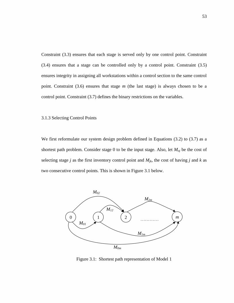
53
Constraint (3.3) ensures that each stage is served only by one control point. Constraint
(3.4) ensures that a stage can be controlled only by a control point. Constraint (3.5)
ensures integrity in assigning all workstations within a control section to the same control
point. Constraint (3.6) ensures that stage m (the last stage) is always chosen to be a
control point. Constraint (3.7) defines the binary restrictions on the variables.
3.1.3 Selecting Control Points
We first reformulate our system design problem defined in Equations (3.2) to (3.7) as a
shortest path problem. Consider stage 0 to be the input stage. Also, let Moj be the cost of
selecting stage j as the first inventory control point and Mjk, the cost of having j and k as
two consecutive control points. This is shown in Figure 3.1 below.
0 1 2 m …………
…
M02
M01
M12
M1m
M2m
M0m
Figure 3.1: Shortest path representation of Model 1
54
Also define
1 if stages and are two consecutive control points
0 otherwiseij
i jx
The ijx ‟s can be thought of as arcs connecting successive control points. Then, the above
formulation ((3.2) to (3.7)) can be modified as follows:
Constraints (3.3) through (3.6) specify that each stage is served by a unique control point.
Additionally, if a stage is chosen as a control point, it serves all stages in between it and
the previous control point. This is analogous to saying that stage m will have exactly one
arc entering into it and none leaving while stages 1 through m-1 will either have no arcs
entering into them and leaving them or exactly one entering and one leaving. Finally,
stage 0 will have one arc leaving it. The formulation (3.2) through (3.7) can therefore be
rewritten in terms of the number of arcs entering and leaving them.
ij ij
i M j M
Min M x
(3.8)
Subject to:
1 if 0
0 if 0 or where , , ,
1 if
ij km
k M
i
x x i m i j k M k i j
i m
j M
(3.9)
[0,1] ,ijx i j M (3.10)

55
If Lj and tj are fixed, 1( )j j j
j M
D L t h
is a constant. If n is fixed, 1
( 1)
2
i m
i M
a D h nk
n
, is a constant for all feasible solutions. Thus, in order to find the optimal solution to the
model, we can ignore these terms from the objective function. In general then:
1, 0,..., 1; 1,...,jk k k j kM f z h j m k j m (3.11)
For this model with predetermined lead times, positive echelon holding costs, and
constant container size, analysis leads to the following result on locating buffers:
Theorem 1: For the cost structure defined in model 1, a single control point is always
optimal if for all stages j=1,…,m-1, 1, 1,j m m j ij m j mf z h h h .
Proof: We will prove the theorem for a two-stage problem and then for a general case
using mathematical induction.
The proof is simple for a two-stage problem. This problem can be represented as shown
in Figure 3.2.
0 1 2 M01 M12
M02
Figure 3.2: Shortest path representation for a two-stage control problem

56
In the figure it is clear that a single control point is optimal if and only if
02 01 12M M M ,
where the costs can be calculated using Equation (3.11). Therefore,
02 2 2 12M f z h , 01 1 1 11M f z h , and 12 2 2 22M f z h .
Substituting in these expressions and rearranging terms, the sufficient condition for a
single control point becomes
1 2 12 1 11 2 22f z h h h (3.12)
Thus, the theorem is true for m = 2.
For an m+1-stage problem, if a single control point is optimal for all k-stage problems
such that k m , we need to consider only the two-arc solutions. This is because any path
to a node k m that uses two or more arcs is dominated. Therefore, for an m+1-stage
problem, a single control point is optimal if:
0, 1 0 , 1 , 1m j j mM M M j M j m (3.13)
Once again we can use Equation (3.11) to compute the costs. Therefore,
0, 1 1 1 1, 1m m m mM f z h , 0 1,j j j jM f z h , and
, 1 1 1 1, 1j m m m j mM f z h .
Substituting the above terms into Equation (3.13) and rearranging terms gives:
1 1, 1 1, 1 1, 1j m m j j m j mf z h h h (3.14)

57
Thus, based on the assumption that the theorem is true for an m-stage problem, it is true
for an m+1-stage problem. Hence it is true for all j M .
In general, the RHS of Equation (3.14) is negative. Since for a, b > 0, a b a b it
can only be positive if the ratio /m jh h , m > j, is large. If we assume that m jh h h , and
noting we are interested in an m state system, Equation (3.14) reduces to:
11 1
1 0 1 0 1
j jm m m m
j m r r j r r m r r
r r r r r j r j
f z h c L t c L t c L t
(3.15)
The right hand side in Equation (3.15) is clearly negative. In this case, a single control
point is always optimal even if there is no fixed cost to maintain an inventory buffer.
58
3.1.4 Choosing Container Size
The formulation in Section 3.1.2 assumed that the batch size, n was known. We now
consider the selection of n. The formulation remains the same, except for one additional
constraint:
max
jn n j M (3.16)
Here, max
jn is the maximum container size that stage j can handle. This would typically be
dictated by the material handling technology or part form at stage j. We will consider
two cases.
Case i) Fixed processing time operations: Here, the production lead time, L is
independent of the container size. In this case the problems of container size and location
of control points are readily seen to be separable in the formulation Equations (3.2) to
(3.7) and (3.16) if we assume a single control point. The results of Askin and Goldberg
(2002) can be extended to multiple stages to conclude *
2 i
i M
m
a D
nh
. If any constraint
(3.16) is violated, then set maxmin j jn n .
Case ii) Variable processing time operations: Here, production lead time is a function of
container size n and is given by the equation: ( )i i iL w s p n
where,

59
is - setup time at stage i.
ip - processing time per unit at stage i.
w - a flow time constant.
In this case, the lead time at a stage is dependent on the container size. WIP cost should
therefore be included in the objective function. The term 1( )j j j
j M
D L t h
is no longer
constant in this case.
For a given n, the model can still be represented as a shortest path problem. Also, since
the container size is fixed across all stages, Theorem 1 is valid for this case too. It is
likely that a single control point will be optimal, thus, a two stage solution approach
seems reasonable. First, determine n. Setting Xm = 1, and Xi = 0, i < m, converts the
objective function into a single variable function that can be readily solved for the
optimal batch size. (The upper bounds for each stage must still be checked for feasibility
and n adjusted accordingly if necessary.) Given n, the Li can be computed and model 1
applied to ensure a single buffer.

60
To determine n, the following heuristics are proposed:
Fixed Point Iterative Heuristic:
To simplify the notation for a general control section, we define j
ij r
r i
P p
and let
1, if stages through form a control section
0, otherwiseij
i jZ
.
The optimal container size can be obtained (as a function of the control structure) by
solving the objective function in Equation (3.2).
The objective function in Equation (3.2) can first be solved as an unconstrained
optimization problem in n and the optimal container size can be determined as
maxmin( *,min )jj M
n n
, where n* is the solution from solving Equation (3.2).
Noting that ( )i i iL w s p n and 1
1
j j
ij j r r
r i r i
c L t
, differentiating Equation (3.2)
with respect to n and setting it to zero, gives:
2
1
02 2
mij j iji m
i i
i M j i j i Mij
Z h Pa D hz w w D h p
n
(3.17)
Therefore:
1
1 1
2
*
2
m
i
i
m mj ij
m ij i i
j i j iij
D a
nh P
h z w Z w D h p
(3.18)
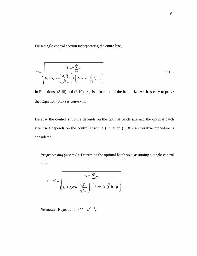
61
For a single control section incorporating the entire line,
1
1
11
2
*
2
m
i
i
mm m
m i i
im
D a
nh P
h z w w D h p
(3.19)
In Equations (3.18) and (3.19), 1m is a function of the batch size n*. It is easy to prove
that Equation (3.17) is convex in n.
Because the control structure depends on the optimal batch size and the optimal batch
size itself depends on the control structure (Equation (3.18)), an iterative procedure is
considered.
Preprocessing (iter = 0): Determine the optimal batch size, assuming a single control
point:
0 1
1
11
2
2
m
i
i
mm m
m i i
im
D a
nh P
h z w w D h p
Iterations: Repeat until niter
= niter-1
:
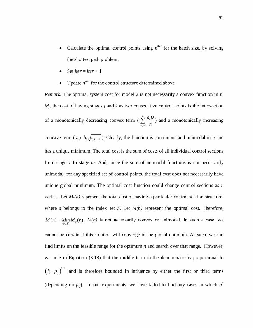
62
Calculate the optimal control points using niter
for the batch size, by solving
the shortest path problem.
Set iter = iter + 1
Update niter
for the control structure determined above
Remark: The optimal system cost for model 2 is not necessarily a convex function in n.
Mjk,the cost of having stages j and k as two consecutive control points is the intersection
of a monotonically decreasing convex term (1
ki
i j
a D
n
) and a monotonically increasing
concave term (1,k j kz h
). Clearly, the function is continuous and unimodal in n and
has a unique minimum. The total cost is the sum of costs of all individual control sections
from stage 1 to stage m. And, since the sum of unimodal functions is not necessarily
unimodal, for any specified set of control points, the total cost does not necessarily have
unique global minimum. The optimal cost function could change control sections as n
varies. Let Ms(n) represent the total cost of having a particular control section structure,
where s belongs to the index set S. Let M(n) represent the optimal cost. Therefore,
{ }( ) ( )s
s SM n Min M n
. M(n) is not necessarily convex or unimodal. In such a case, we
cannot be certain if this solution will converge to the global optimum. As such, we can
find limits on the feasible range for the optimum n and search over that range. However,
we note in Equation (3.18) that the middle term in the denominator is proportional to
1/ 2
i ijh p and is therefore bounded in influence by either the first or third terms
(depending on pij). In our experiments, we have failed to find any cases in which n*
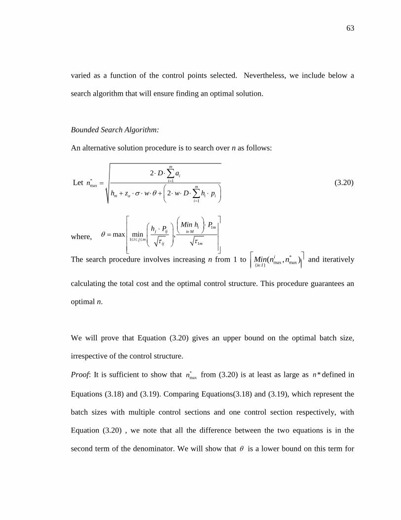
63
varied as a function of the control points selected. Nevertheless, we include below a
search algorithm that will ensure finding an optimal solution.
Bounded Search Algorithm:
An alternative solution procedure is to search over n as follows:
Let * 1max
1
2
2
m
i
i
m
m i i
i
D a
n
h z w w D h p
(3.20)
where,
The search procedure involves increasing n from 1 to *
max max{ }
( , )i
i IMin n n
and iteratively
calculating the total cost and the optimal control structure. This procedure guarantees an
optimal n.
We will prove that Equation (3.20) gives an upper bound on the optimal batch size,
irrespective of the control structure.
Proof: It is sufficient to show that *
maxn from (3.20) is at least as large as *n defined in
Equations (3.18) and (3.19). Comparing Equations(3.18) and (3.19), which represent the
batch sizes with multiple control sections and one control section respectively, with
Equation (3.20) , we note that all the difference between the two equations is in the
second term of the denominator. We will show that is a lower bound on this term for
1
11
max min ,i m
j ij i M
i j mij m
Min h Ph P
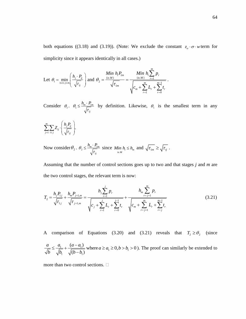
64
both equations ((3.18) and (3.19)). (Note: We exclude the constant z w term for
simplicity since it appears identically in all cases.)
Let 11min
j ij
i j mij
h P
and 1
{ }{ } 12
11
1 0
m
i ri mi Mi M r
m mm
m r r
r r
Min h pMin h P
c L t
.
Consider 1 . 1
1m m
ij
h P
by definition. Likewise,
1 is the smallest term in any
1
mj ij
ij
j i j ij
h PZ
.
Now consider 2 . 12
m m
ij
h P
since i m
i M
Min h h
and 1m ij .
Assuming that the number of control sections goes up to two and that stages j and m are
the two control stages, the relevant term is now:
1 1, 112
1 11 1,
11 0
mj
m rj rj j m j m r jr
j j m mj j m
m r rj r rr j r jr r
h ph ph P h P
T
c L tc L t
(3.21)
A comparison of Equations (3.20) and (3.21) reveals that 2 2T (since
1 11 1
1 1
( )where 0, 0
( )
a a aaa a b b
b b b b
). The proof can similarly be extended to
more than two control sections.

65
3.2 Model 2: Section Dependent Container Size
We no longer assume that the container sizes are constant across stages; each control
section selects a container size. All the other assumptions for model 1 apply. Since an
entire container must be removed at a time from the output buffer and likewise we
assume that an entire container is started into production instantaneously at the beginning
of a control section, there should be a nesting relationship. The upstream container size
is an integer multiple of that used in its immediate downstream section, i.e. 1
1j j jn r n
for some non-negative integer rj. (Note, following the work or Roundy (1986), rj may be
restricted to powers of two with limited loss). Remaining units from the partially
emptied upstream container are kept as input staging at the downstream section until
needed.
The objective function for this model will now be:
1
1
1
(1 ) ( 1)
2 2
( )
j j j ji m mj j
j M i M j Mij j
j i
j j ij ij i i i
j M i j i M
h X n ra D h nMin f X
Y n
z h X Y h L t D
(3.22)
where jn is the container size at stage j.
In addition to the constraints in model 1, we have:
max ; ; 1,...,j ij in Y n j M i j (3.23)
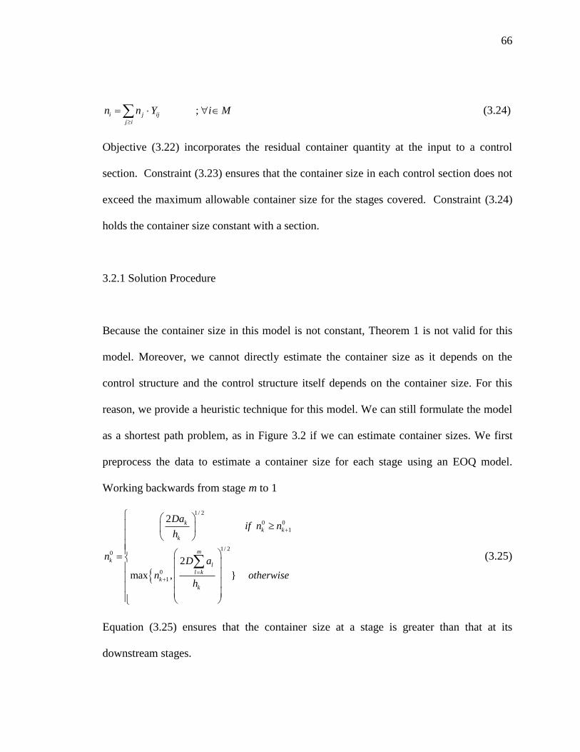
66
; i j ij
j i
n n Y i M
(3.24)
Objective (3.22) incorporates the residual container quantity at the input to a control
section. Constraint (3.23) ensures that the container size in each control section does not
exceed the maximum allowable container size for the stages covered. Constraint (3.24)
holds the container size constant with a section.
3.2.1 Solution Procedure
Because the container size in this model is not constant, Theorem 1 is not valid for this
model. Moreover, we cannot directly estimate the container size as it depends on the
control structure and the control structure itself depends on the container size. For this
reason, we provide a heuristic technique for this model. We can still formulate the model
as a shortest path problem, as in Figure 3.2 if we can estimate container sizes. We first
preprocess the data to estimate a container size for each stage using an EOQ model.
Working backwards from stage m to 1
1/ 2
0 0
1
1/ 20
0
1
2
2
max , }
k
k k
k
m
kl
l k
k
k
Daif n n
h
n D a
n otherwiseh
(3.25)
Equation (3.25) ensures that the container size at a stage is greater than that at its
downstream stages.
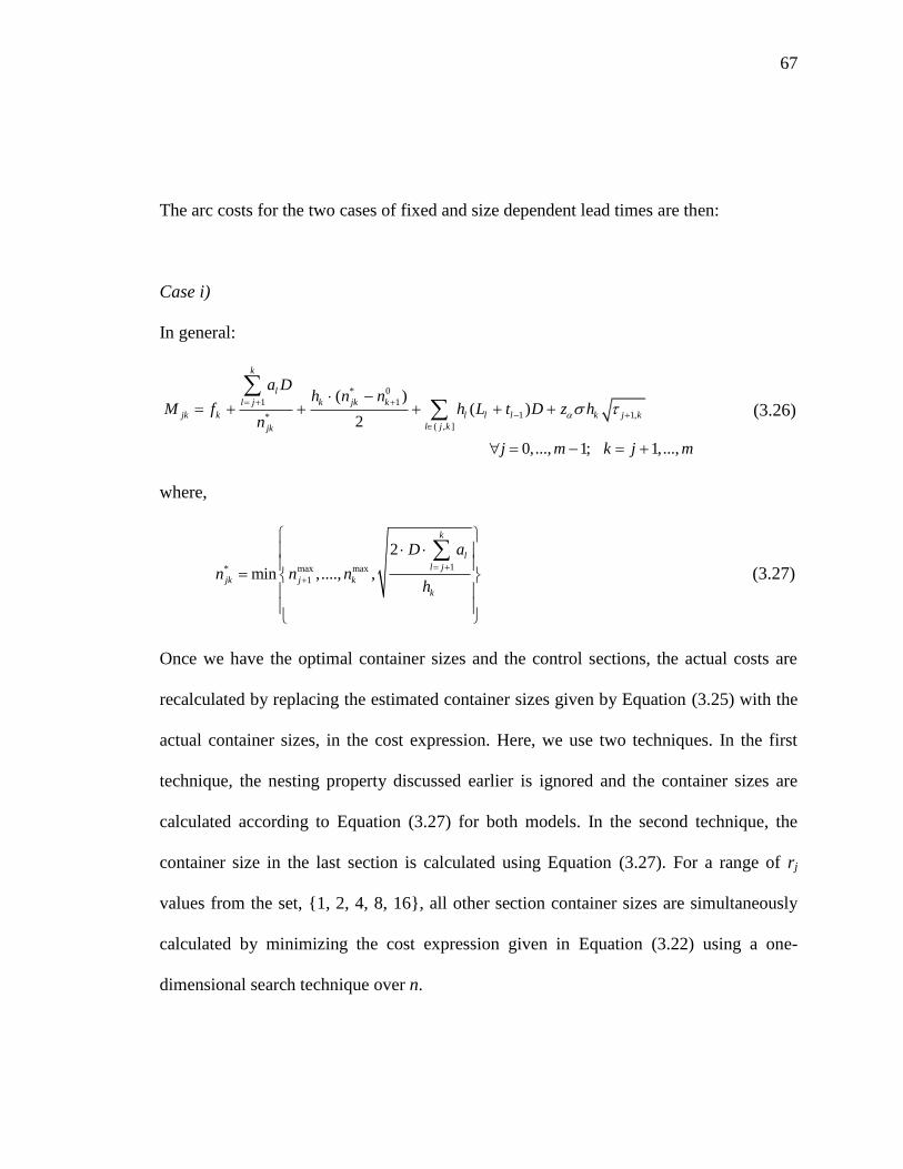
67
The arc costs for the two cases of fixed and size dependent lead times are then:
Case i)
In general:
* 0
1 1
1 1,*( , ]
( )( )
2
0,..., 1; 1,...,
k
l
l j k jk k
jk k l l l k j k
l j kjk
a Dh n n
M f h L t D z hn
j m k j m
(3.26)
where,
1* max max
1
2
min ,...., ,
k
l
l j
jk j k
k
D a
n n nh
(3.27)
Once we have the optimal container sizes and the control sections, the actual costs are
recalculated by replacing the estimated container sizes given by Equation (3.25) with the
actual container sizes, in the cost expression. Here, we use two techniques. In the first
technique, the nesting property discussed earlier is ignored and the container sizes are
calculated according to Equation (3.27) for both models. In the second technique, the
container size in the last section is calculated using Equation (3.27). For a range of rj
values from the set, {1, 2, 4, 8, 16}, all other section container sizes are simultaneously
calculated by minimizing the cost expression given in Equation (3.22) using a one-
dimensional search technique over n.

68
Theorem 1 can be modified for evaluating the shortest path model in this case.
Theorem 2: For the cost structure defined in model 2 a single control point is always
optimal, i.e., stage m is the only control point, if for all stages j,
* *
1 0, ,1 1
* * *
0, 0, ,
* 0
0, 1
1, 1, 1,
( )
2
( )
2
mjm
ll ll j m m j ml l
j
m j j m
j j j
m m j j m j k
a Da a Dh n n
f Dn n n
h n nz h h h
.
Proof: The proof follows the same procedure used in Theorem 1.
Case ii) The only difference between Case (i) and Case (ii) is that the lead time depends
on the container size in Case (ii). Arguments similar to those used in Theorem 2 can be
applied to Case (ii) after including WIP cost. However, the difference is in the
calculation of the optimal container size at each control section. In general:
* 0
1 1 *
1,*1
( )( )
2
0,1,..., 1; 1,...,
k
l kl j k jk k
jk k l l jk k j k
l jjk
a Dh n n
M f h L n D z hn
j m k j m
(3.28)
where, *
jkn can be determined by minimizing:
0
1 1
1 1,
1
( )( ) ( ( ) )
2
0,1,..., 1; 1,...,
k
l kl j k jk k
jk l l jk l k j k
l jjk
a Dh n n
f n h L n t D z hn
j m k j m
(3.29)
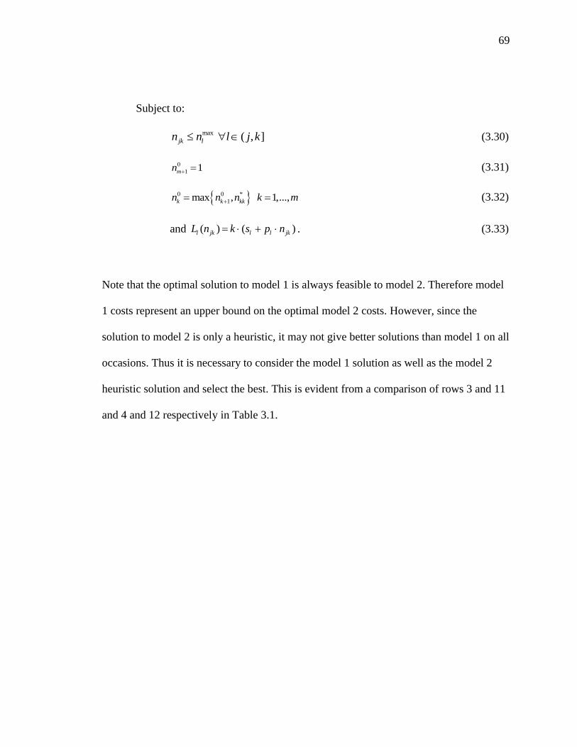
69
Subject to:
max ( , ]jk ln n l j k (3.30)
0
1 1mn (3.31)
0 0 *
1max , 1,...,k k kkn n n k m (3.32)
and ( ) ( )l jk l l jkL n k s p n . (3.33)
Note that the optimal solution to model 1 is always feasible to model 2. Therefore model
1 costs represent an upper bound on the optimal model 2 costs. However, since the
solution to model 2 is only a heuristic, it may not give better solutions than model 1 on all
occasions. Thus it is necessary to consider the model 1 solution as well as the model 2
heuristic solution and select the best. This is evident from a comparison of rows 3 and 11
and 4 and 12 respectively in Table 3.1.
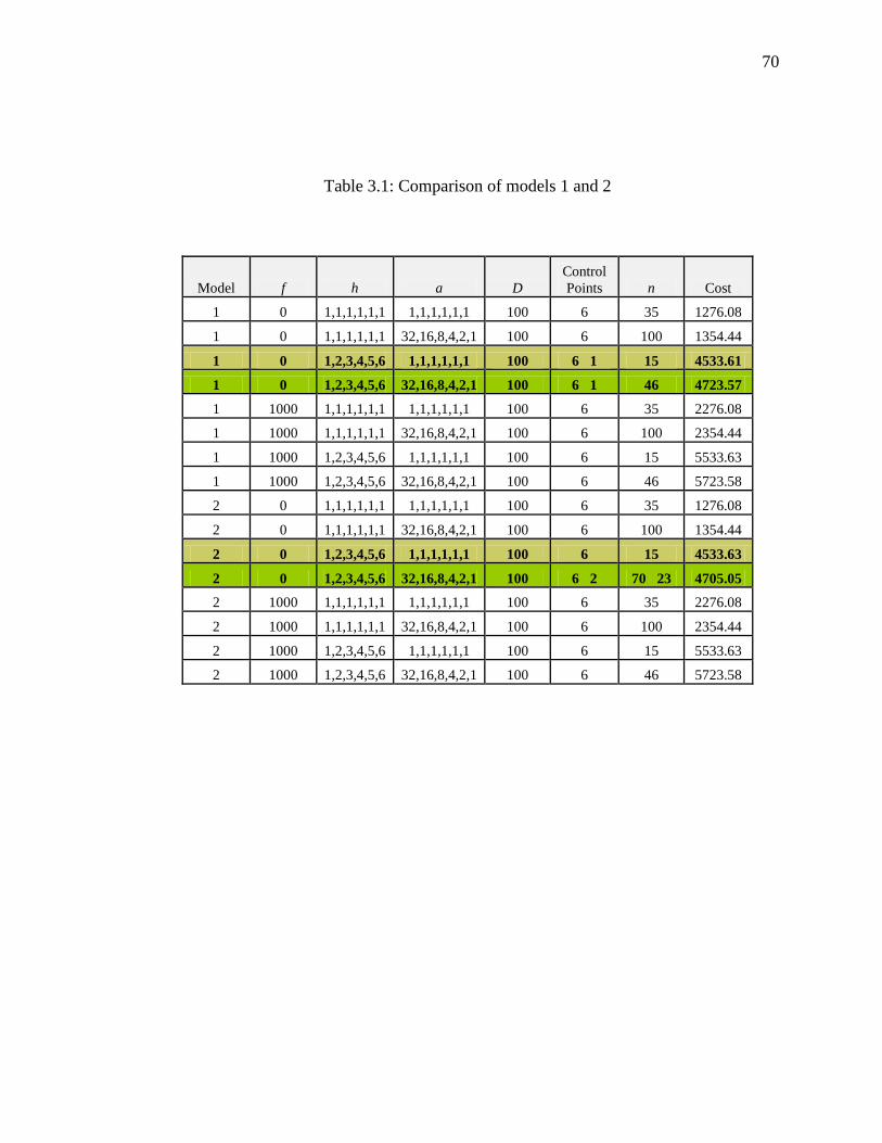
70
Table 3.1: Comparison of models 1 and 2
Model f h a D
Control
Points n Cost
1 0 1,1,1,1,1,1 1,1,1,1,1,1 100 6 35 1276.08
1 0 1,1,1,1,1,1 32,16,8,4,2,1 100 6 100 1354.44
1 0 1,2,3,4,5,6 1,1,1,1,1,1 100 6 1 15 4533.61
1 0 1,2,3,4,5,6 32,16,8,4,2,1 100 6 1 46 4723.57
1 1000 1,1,1,1,1,1 1,1,1,1,1,1 100 6 35 2276.08
1 1000 1,1,1,1,1,1 32,16,8,4,2,1 100 6 100 2354.44
1 1000 1,2,3,4,5,6 1,1,1,1,1,1 100 6 15 5533.63
1 1000 1,2,3,4,5,6 32,16,8,4,2,1 100 6 46 5723.58
2 0 1,1,1,1,1,1 1,1,1,1,1,1 100 6 35 1276.08
2 0 1,1,1,1,1,1 32,16,8,4,2,1 100 6 100 1354.44
2 0 1,2,3,4,5,6 1,1,1,1,1,1 100 6 15 4533.63
2 0 1,2,3,4,5,6 32,16,8,4,2,1 100 6 2 70 23 4705.05
2 1000 1,1,1,1,1,1 1,1,1,1,1,1 100 6 35 2276.08
2 1000 1,1,1,1,1,1 32,16,8,4,2,1 100 6 100 2354.44
2 1000 1,2,3,4,5,6 1,1,1,1,1,1 100 6 15 5533.63
2 1000 1,2,3,4,5,6 32,16,8,4,2,1 100 6 46 5723.58
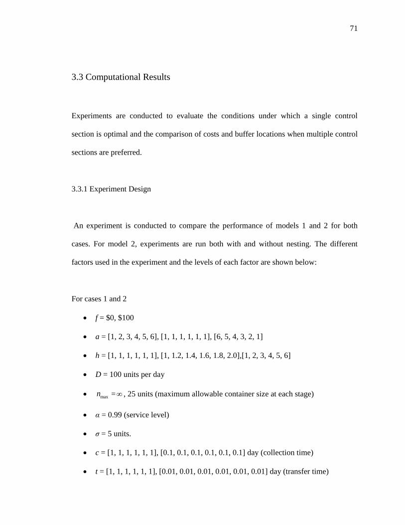
71
3.3 Computational Results
Experiments are conducted to evaluate the conditions under which a single control
section is optimal and the comparison of costs and buffer locations when multiple control
sections are preferred.
3.3.1 Experiment Design
An experiment is conducted to compare the performance of models 1 and 2 for both
cases. For model 2, experiments are run both with and without nesting. The different
factors used in the experiment and the levels of each factor are shown below:
For cases 1 and 2
f = $0, $100
a = [1, 2, 3, 4, 5, 6], [1, 1, 1, 1, 1, 1], [6, 5, 4, 3, 2, 1]
h = [1, 1, 1, 1, 1, 1], [1, 1.2, 1.4, 1.6, 1.8, 2.0],[1, 2, 3, 4, 5, 6]
D = 100 units per day
maxn = , 25 units (maximum allowable container size at each stage)
α = 0.99 (service level)
σ = 5 units.
c = [1, 1, 1, 1, 1, 1], [0.1, 0.1, 0.1, 0.1, 0.1, 0.1] day (collection time)
t = [1, 1, 1, 1, 1, 1], [0.01, 0.01, 0.01, 0.01, 0.01, 0.01] day (transfer time)

72
For case 1
L = [1, 1, 1, 1, 1, 1], [0.1, 0.1, 0.1, 0.1, 0.1, 0.1] days (case 1 production lead time)
For case 2
s = 0.05
p = 0.005
w = 1
Therefore, a total of 288 runs are carried out for case 1 of each model and 144 runs for
case 2. The programs are written in C++. Golden Section Search is used to determine the
batch size for case 2 of both models. Each run took less than one second to run.
3.3.2 Discussion of Results
An analysis of the results of the experiments shows that for case 1, for both models 1 and
2, the average cost is around $1495, and for case 2, it is around $1714. The costs for both
models are approximately equal because in a majority of the experiments, model 1 and
model 2 gave similar solutions. Table 3.2 below summarizes the results of the analysis.
The table indicates that model 2 does not increase the number of control points in most
cases, especially for Case 1. From row 3 of the table it is evident that this occurs only
once for case 1 and only fourteen times for case 2, whereas, from row 4 it is evident that
model 2 reduces costs by having different container sizes in different control sections,
five times and twenty times for Case 1 and Case 2 respectively.
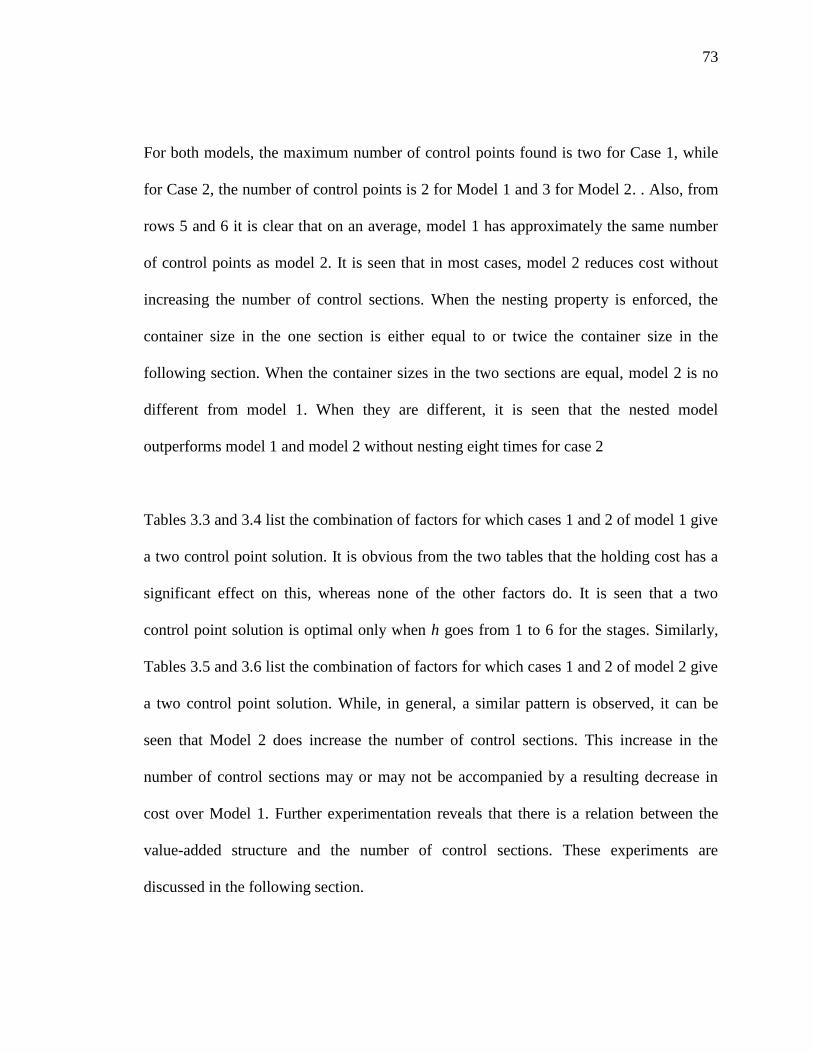
73
For both models, the maximum number of control points found is two for Case 1, while
for Case 2, the number of control points is 2 for Model 1 and 3 for Model 2. . Also, from
rows 5 and 6 it is clear that on an average, model 1 has approximately the same number
of control points as model 2. It is seen that in most cases, model 2 reduces cost without
increasing the number of control sections. When the nesting property is enforced, the
container size in the one section is either equal to or twice the container size in the
following section. When the container sizes in the two sections are equal, model 2 is no
different from model 1. When they are different, it is seen that the nested model
outperforms model 1 and model 2 without nesting eight times for case 2
Tables 3.3 and 3.4 list the combination of factors for which cases 1 and 2 of model 1 give
a two control point solution. It is obvious from the two tables that the holding cost has a
significant effect on this, whereas none of the other factors do. It is seen that a two
control point solution is optimal only when h goes from 1 to 6 for the stages. Similarly,
Tables 3.5 and 3.6 list the combination of factors for which cases 1 and 2 of model 2 give
a two control point solution. While, in general, a similar pattern is observed, it can be
seen that Model 2 does increase the number of control sections. This increase in the
number of control sections may or may not be accompanied by a resulting decrease in
cost over Model 1. Further experimentation reveals that there is a relation between the
value-added structure and the number of control sections. These experiments are
discussed in the following section.
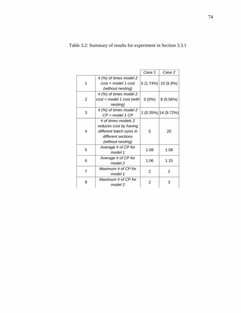
74
Table 3.2: Summary of results for experiment in Section 3.3.1
Case 1 Case 2
1
# (%) of times model 2
cost < model 1 cost
(without nesting)
5 (1.74%) 10 (6.9%)
2
# (%) of times model 2
cost < model 1 cost (with
nesting)
0 (0%) 8 (5.56%)
3 # (%) of times model 2
CP > model 1 CP 1 (0.35%) 14 (9.72%)
4
# of times models 2
reduces cost by having
different batch sizes in
different sections
(without nesting)
5 20
5 Average # of CP for
model 1 1.08 1.08
6 Average # of CP for
model 2 1.06 1.15
7 Maximum # of CP for
model 1 2 2
8 Maximum # of CP for
model 2 2 3
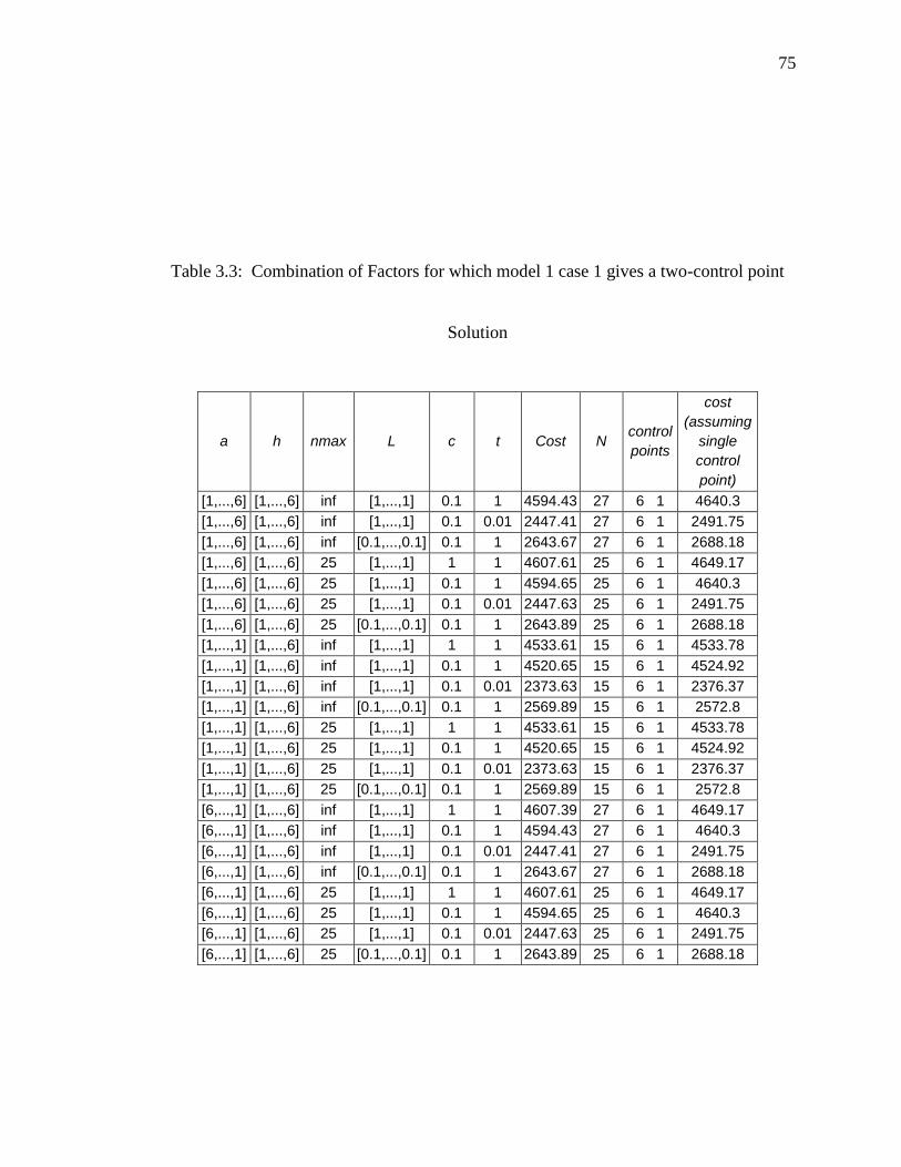
75
Table 3.3: Combination of Factors for which model 1 case 1 gives a two-control point
Solution
a h nmax L c t Cost N control
points
cost
(assuming
single
control
point)
[1,...,6] [1,...,6] inf [1,...,1] 0.1 1 4594.43 27 6 1 4640.3
[1,...,6] [1,...,6] inf [1,...,1] 0.1 0.01 2447.41 27 6 1 2491.75
[1,...,6] [1,...,6] inf [0.1,...,0.1] 0.1 1 2643.67 27 6 1 2688.18
[1,...,6] [1,...,6] 25 [1,...,1] 1 1 4607.61 25 6 1 4649.17
[1,...,6] [1,...,6] 25 [1,...,1] 0.1 1 4594.65 25 6 1 4640.3
[1,...,6] [1,...,6] 25 [1,...,1] 0.1 0.01 2447.63 25 6 1 2491.75
[1,...,6] [1,...,6] 25 [0.1,...,0.1] 0.1 1 2643.89 25 6 1 2688.18
[1,...,1] [1,...,6] inf [1,...,1] 1 1 4533.61 15 6 1 4533.78
[1,...,1] [1,...,6] inf [1,...,1] 0.1 1 4520.65 15 6 1 4524.92
[1,...,1] [1,...,6] inf [1,...,1] 0.1 0.01 2373.63 15 6 1 2376.37
[1,...,1] [1,...,6] inf [0.1,...,0.1] 0.1 1 2569.89 15 6 1 2572.8
[1,...,1] [1,...,6] 25 [1,...,1] 1 1 4533.61 15 6 1 4533.78
[1,...,1] [1,...,6] 25 [1,...,1] 0.1 1 4520.65 15 6 1 4524.92
[1,...,1] [1,...,6] 25 [1,...,1] 0.1 0.01 2373.63 15 6 1 2376.37
[1,...,1] [1,...,6] 25 [0.1,...,0.1] 0.1 1 2569.89 15 6 1 2572.8
[6,...,1] [1,...,6] inf [1,...,1] 1 1 4607.39 27 6 1 4649.17
[6,...,1] [1,...,6] inf [1,...,1] 0.1 1 4594.43 27 6 1 4640.3
[6,...,1] [1,...,6] inf [1,...,1] 0.1 0.01 2447.41 27 6 1 2491.75
[6,...,1] [1,...,6] inf [0.1,...,0.1] 0.1 1 2643.67 27 6 1 2688.18
[6,...,1] [1,...,6] 25 [1,...,1] 1 1 4607.61 25 6 1 4649.17
[6,...,1] [1,...,6] 25 [1,...,1] 0.1 1 4594.65 25 6 1 4640.3
[6,...,1] [1,...,6] 25 [1,...,1] 0.1 0.01 2447.63 25 6 1 2491.75
[6,...,1] [1,...,6] 25 [0.1,...,0.1] 0.1 1 2643.89 25 6 1 2688.18
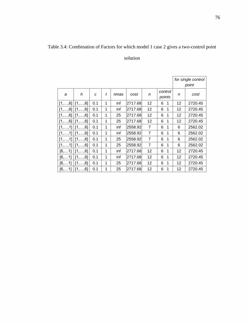
76
Table 3.4: Combination of Factors for which model 1 case 2 gives a two-control point
solution
for single control
point
a h c t nmax cost n control
points n cost
[1,…,6] [1,…,6] 0.1 1 inf 2717.68 12 6 1 12 2720.45
[1,…,6] [1,…,6] 0.1 1 inf 2717.68 12 6 1 12 2720.45
[1,…,6] [1,…,6] 0.1 1 25 2717.68 12 6 1 12 2720.45
[1,…,6] [1,…,6] 0.1 1 25 2717.68 12 6 1 12 2720.45
[1,…,1] [1,…,6] 0.1 1 inf 2558.92 7 6 1 6 2562.02
[1,…,1] [1,…,6] 0.1 1 inf 2558.92 7 6 1 6 2562.02
[1,…,1] [1,…,6] 0.1 1 25 2558.92 7 6 1 6 2562.02
[1,…,1] [1,…,6] 0.1 1 25 2558.92 7 6 1 6 2562.02
[6,…1] [1,…,6] 0.1 1 inf 2717.68 12 6 1 12 2720.45
[6,…1] [1,…,6] 0.1 1 inf 2717.68 12 6 1 12 2720.45
[6,…1] [1,…,6] 0.1 1 25 2717.68 12 6 1 12 2720.45
[6,…1] [1,…,6] 0.1 1 25 2717.68 12 6 1 12 2720.45

77
Table 3.5: Combination of Factors for which model 2 case 1 gives a two-control point
solution
For single
control point
a h nmax L c t Cost n control
points n cost
[1,...,6] [1,...,6] inf [1,...,1] 0.1 1 4594.42 26 26 6 1 27 4640.3
[1,...,6] [1,...,6] 25 [1,...,1] 0.1 1 4594.65 25 25 6 1 25 4640.3
[1,...,6] [1,...,6] 25 [0.1,...,0.1] 0.1 1 2643.89 25 25 6 1 25 2688.18
[1,...,1] [1,...,6] inf [1,...,1] 0.1 1 4520.8 13 13 6 1 15 4524.92
[1,...,1] [1,...,6] inf [1,...,1] 0.1 0.01 2373.78 13 13 6 1 15 2376.37
[1,...,1] [1,...,6] inf [0.1,...,0.1] 0.1 1 2570.05 13 13 6 1 15 2572.8
[1,...,1] [1,...,6] 25 [1,...,1] 0.1 1 4520.8 13 13 6 1 15 4524.92
[1,...,1] [1,...,6] 25 [1,...,1] 0.1 0.01 2373.78 13 13 6 1 15 2376.37
[1,...,1] [1,...,6] 25 [0.1,...,0.1] 0.1 1 2570.05 13 13 6 1 15 2572.8
[6,...,1] [1,...,6] inf [1,...,1] 1 1 4607.37 46 23 6 1 27 4649.17
[6,...,1] [1,...,6] inf [1,...,1] 0.1 1 4594.41 46 23 6 1 27 4640.3
[6,...,1] [1,...,6] inf [1,...,1] 0.1 0.01 2447.39 46 23 6 1 27 2491.75
[6,...,1] [1,...,6] inf [0.1,...,0.1] 0.1 1 2643.65 46 23 6 1 27 2688.18
[6,...,1] [1,...,6] inf [0.1,...,0.1] 0.1 0.01 448.357 46 23 6 1 27 489.379
[6,...,1] [1,...,6] 25 [1,...,1] 0.1 1 4594.41 46 23 6 1 25 4640.3
[6,...,1] [1,...,6] 25 [1,...,1] 0.1 0.01 2447.39 46 23 6 1 25 2491.75
[6,...,1] [1,...,6] 25 [0.1,...,0.1] 0.1 1 2643.65 46 23 6 1 25 2688.18
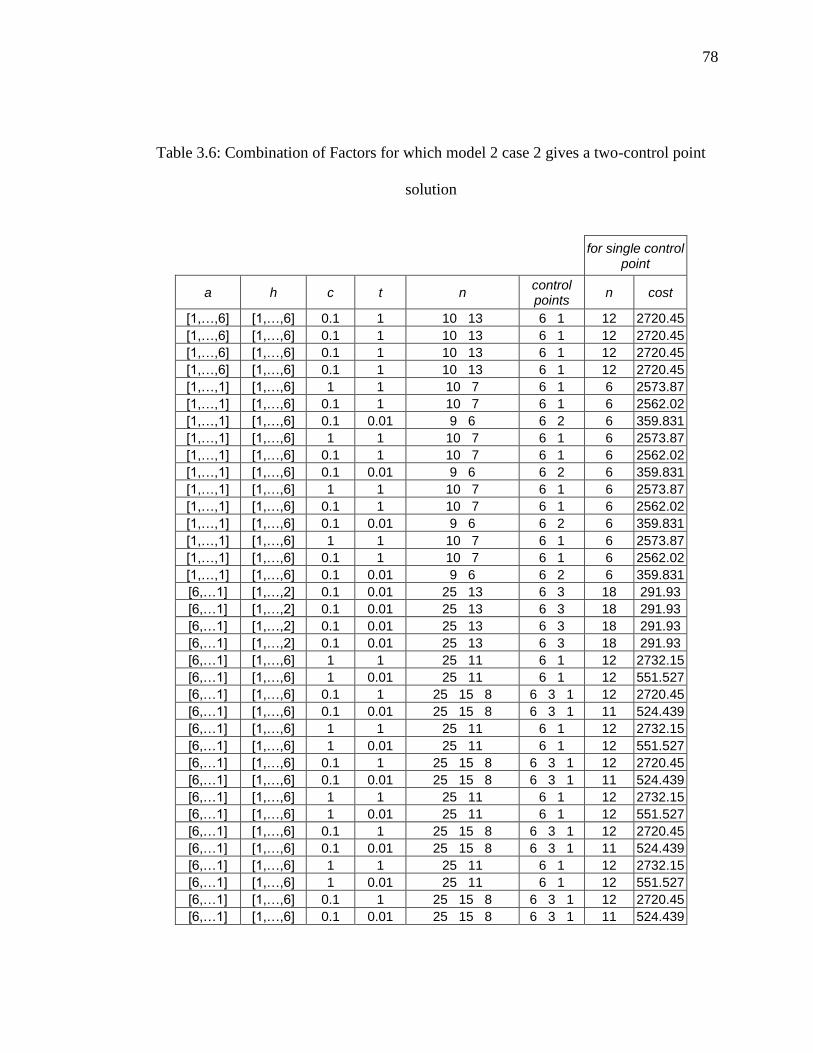
78
Table 3.6: Combination of Factors for which model 2 case 2 gives a two-control point
solution
for single control
point
a h c t n control points
n cost
[1,…,6] [1,…,6] 0.1 1 10 13 6 1 12 2720.45
[1,…,6] [1,…,6] 0.1 1 10 13 6 1 12 2720.45
[1,…,6] [1,…,6] 0.1 1 10 13 6 1 12 2720.45
[1,…,6] [1,…,6] 0.1 1 10 13 6 1 12 2720.45
[1,…,1] [1,…,6] 1 1 10 7 6 1 6 2573.87
[1,…,1] [1,…,6] 0.1 1 10 7 6 1 6 2562.02
[1,…,1] [1,…,6] 0.1 0.01 9 6 6 2 6 359.831
[1,…,1] [1,…,6] 1 1 10 7 6 1 6 2573.87
[1,…,1] [1,…,6] 0.1 1 10 7 6 1 6 2562.02
[1,…,1] [1,…,6] 0.1 0.01 9 6 6 2 6 359.831
[1,…,1] [1,…,6] 1 1 10 7 6 1 6 2573.87
[1,…,1] [1,…,6] 0.1 1 10 7 6 1 6 2562.02
[1,…,1] [1,…,6] 0.1 0.01 9 6 6 2 6 359.831
[1,…,1] [1,…,6] 1 1 10 7 6 1 6 2573.87
[1,…,1] [1,…,6] 0.1 1 10 7 6 1 6 2562.02
[1,…,1] [1,…,6] 0.1 0.01 9 6 6 2 6 359.831
[6,…1] [1,…,2] 0.1 0.01 25 13 6 3 18 291.93
[6,…1] [1,…,2] 0.1 0.01 25 13 6 3 18 291.93
[6,…1] [1,…,2] 0.1 0.01 25 13 6 3 18 291.93
[6,…1] [1,…,2] 0.1 0.01 25 13 6 3 18 291.93
[6,…1] [1,…,6] 1 1 25 11 6 1 12 2732.15
[6,…1] [1,…,6] 1 0.01 25 11 6 1 12 551.527
[6,…1] [1,…,6] 0.1 1 25 15 8 6 3 1 12 2720.45
[6,…1] [1,…,6] 0.1 0.01 25 15 8 6 3 1 11 524.439
[6,…1] [1,…,6] 1 1 25 11 6 1 12 2732.15
[6,…1] [1,…,6] 1 0.01 25 11 6 1 12 551.527
[6,…1] [1,…,6] 0.1 1 25 15 8 6 3 1 12 2720.45
[6,…1] [1,…,6] 0.1 0.01 25 15 8 6 3 1 11 524.439
[6,…1] [1,…,6] 1 1 25 11 6 1 12 2732.15
[6,…1] [1,…,6] 1 0.01 25 11 6 1 12 551.527
[6,…1] [1,…,6] 0.1 1 25 15 8 6 3 1 12 2720.45
[6,…1] [1,…,6] 0.1 0.01 25 15 8 6 3 1 11 524.439
[6,…1] [1,…,6] 1 1 25 11 6 1 12 2732.15
[6,…1] [1,…,6] 1 0.01 25 11 6 1 12 551.527
[6,…1] [1,…,6] 0.1 1 25 15 8 6 3 1 12 2720.45
[6,…1] [1,…,6] 0.1 0.01 25 15 8 6 3 1 11 524.439
79
3.3.3 Effect of Value Added Structure on Number of Control Sections
From theorems 1 and 2, it is clear that the number of control points is dependent on the
value added structure and to a much lesser extent on the lead times. In this section we
perform a small experiment on a 20-stage pull system. Fixed parameters for the
experiment are as follows:
f = $0
a = [1, 2, 3, … ,20]
D = 100 units per day
maxn = (maximum allowable container size at each stage)
α = 0.99 (service level)
σ = 5 units.
c = [0.1, 0.1, …. ,0.1] day (collection time)
t = [1, 1, …… ,1] day (transfer time)
The value added structure is carried for the experiment. We consider only case 1 of
model 1 because of the similarity between the control structures obtained using models 1
and 2. The results are displayed in Table 3.7. For the parameters described above, when
the increase in holding costs is gradual, there are only 2 control points. For example,
whether the holding costs go from 1 to 20 in steps of 1 or from 1 to 1000 in steps of 50, a
two control point solution is optimal. However, when the holding costs are [1, 2,…19,
24] stages 1, 4, and 20 are selected as control points. When the holding costs are [1, 2, …

80
19, 25 (and above)], the optimal solution changes to 2, 19, and 20 as control points.
Clearly, the holding cost at the final stage has a significant impact on the control
structure. In a postponement type strategy where the maximum value-added strategies are
carried out at the end, the model tries to push more control points to the end.
When the holding cost increases in batches, with the first five stages having a holding
cost of 1, the next five having a holding cost of 50, the next five 100, and the final five
150 ([1,...,1,50,…,50,100,…,100,150,…150]), the result is similar to the gradually
increasing holding cost case. A two control point solution is optimal with control points
at stages 5 and 20. When we have a structure where the holding cost for the first ten
stages is 50 and for the next ten stages is 100, a single control point is optimal. However,
when the holding cost for the next ten stages increases above 130, two control points are
setup at stages 10 and 20. The same solution is obtained when only the holding cost at the
final stage is changed to 130. and locations will stay the same or move downstream.
From Equation (3.14) it is clear that a single control point is optimal if:
1 1,
j j ij
m
m m
f z hh
z
for all j M . In all of our test cases, the algorithm places a
control point at the first stage where this constraint is violated.
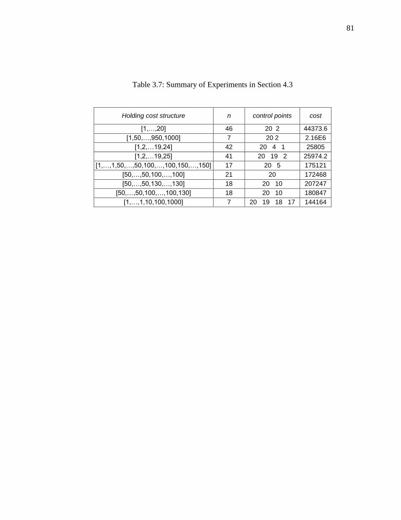
81
Table 3.7: Summary of Experiments in Section 4.3
Holding cost structure n control points cost
[1,…,20] 46 20 2 44373.6
[1,50,…,950,1000] 7 20 2 2.16E6
[1,2,…19,24] 42 20 4 1 25805
[1,2,…19,25] 41 20 19 2 25974.2
[1,…,1,50,…,50,100,…,100,150,…,150] 17 20 5 175121
[50,…,50,100,…,100] 21 20 172468
[50,…,50,130,…,130] 18 20 10 207247
[50,…,50,100,…,100,130] 18 20 10 180847
[1,…,1,10,100,1000] 7 20 19 18 17 144164
82
CHAPTER 4: MULTI-PRODUCT STOCHASTIC MODEL
4.1 Introduction
In the previous chapter, we discussed the issue of locating control points for a shop
manufacturing a single part type, where the part visits each machine once. Queuing
aspects were not considered. Processing times were assumed to be deterministic. In this
chapter, we extend the models in the previous chapter to a multi-product serial system.
Service times and demand interarrival times are now assumed to be random. We assume
that sufficient average capacity is available. Since more than one product type is
produced, the products compete with each other for the limited machine resources. This
results in an increase in the production lead time mean and variance at each stage as
compared to the models in the previous chapter. This increase is due to the additional
time spent by each part, waiting for service. We still assume a serial product flowing
through all stages, i.e., product merge/split issues are not considered. We model the
system as a GI/G/1 queue and determine the approximate waiting times by using a
Decomposition/Recomposition Technique modeled after Shantikumar and Buzacott
(1981). We then build a simulation model to test the accuracy of our expression. This
model is described in Chapter 5. Although an approximation, we believe that an open
queueing network model for flow between stages within a control section will be accurate
unless the system is consistently operating above capacity. Since we have assumed
sufficient average capacity, this situation will not occur too often.

83
4.2 Assumptions
All products have the same set of control points. This assumption is reasonable
because it makes the system easier to operate when the manufacturing system
produces a large number of parts.
All products have the same serial flow. The modeling assumption is applicable for
p distinct products or p customized versions of a single product type.
Sufficient average capacity is available.
Raw materials are always available.
The waiting time for a transporter is assumed to be known.
FCFS queuing discipline is assumed.

84
4.3 Model Formulation
The notation used in this model is as follows:
p - product index (p = 1…P)
ci - collection time for kanbans at stage i
( )pf d - probability density function of demand per time for product p at stage m.
2( ) , ( )p p p p pE D V
if - Fixed cost per time for locating and maintaining inventory at stage i
- Percentage of orders satisfied without delay (service rate)
z - Standard Normal Variate such that { }P Z Z
M - Set of all stages {1, …., m}
iph - Inventory holding cost per unit per period of product p at stage i, i M
ipL - Production Lead time at stage i for product p (total time spent by each unit of
product p at machine i)
ti - transport time from stage i to stage i+1 (including time to wait for move if
applicable)
iX - 1 if stage is a control point
0 otherwise
i
ijY - 1 if stage is a control point that serves stage
0 otherwise
j i
ijY defined for , 1,....,j i i m

85
ipa - Setup cost plus material handling cost per container of product p at stage i
pn - Container size for product p
ijp - Lead time from stage i to stage j for product p, defined for i being the first stage in a
control section
ip - Processing time for each unit of product p at machine i
ipS - Setup time for part p at machine i
iqW - Expected average waiting time (in queue) at machine i
ip - Average arrival rate of product p containers at machine i
ip - Average service rate of product p containers at machine i
i - Traffic intensity at machine i
In order to determine the control structure, we need to know the container size for each
product. We use a model, similar to the ones described in Karmarkar et al (1985) and
Karmarkar (1987). We first determine the expected waiting time and processing time for
each part type at each machine separately. The equations are as follows:
( )iip q ip p ipL W S n (4.1)
1
1
j j
ijp j rp r
r i r i
c L t
(4.2)
p
ip
p
D
n
(4.3)
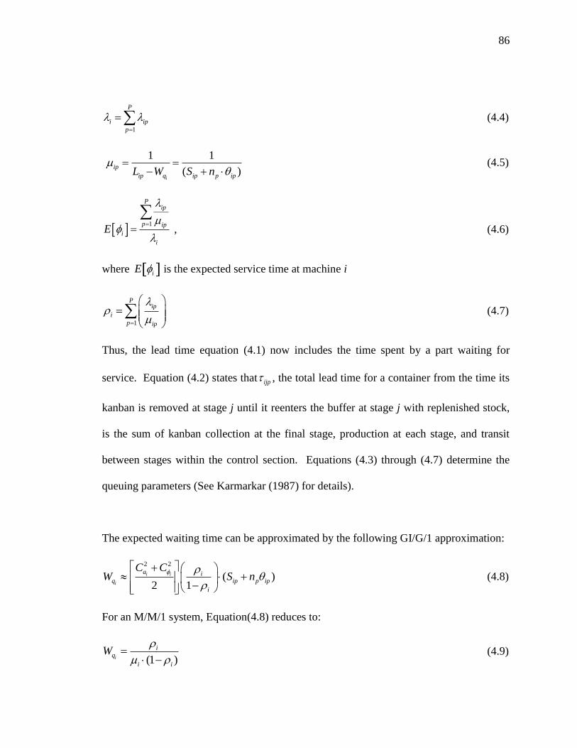
86
1
P
i ip
p
(4.4)
1 1
( )i
ip
ip q ip p ipL W S n
(4.5)
1
Pip
p ip
i
i
E
, (4.6)
where iE is the expected service time at machine i
1
Pip
i
p ip
(4.7)
Thus, the lead time equation (4.1) now includes the time spent by a part waiting for
service. Equation (4.2) states that ijp , the total lead time for a container from the time its
kanban is removed at stage j until it reenters the buffer at stage j with replenished stock,
is the sum of kanban collection at the final stage, production at each stage, and transit
between stages within the control section. Equations (4.3) through (4.7) determine the
queuing parameters (See Karmarkar (1987) for details).
The expected waiting time can be approximated by the following GI/G/1 approximation:
2 2
( )2 1
i i
i
a iq ip p ip
i
C CW S n
(4.8)
For an M/M/1 system, Equation(4.8) reduces to:
(1 )i
iq
i i
W
(4.9)
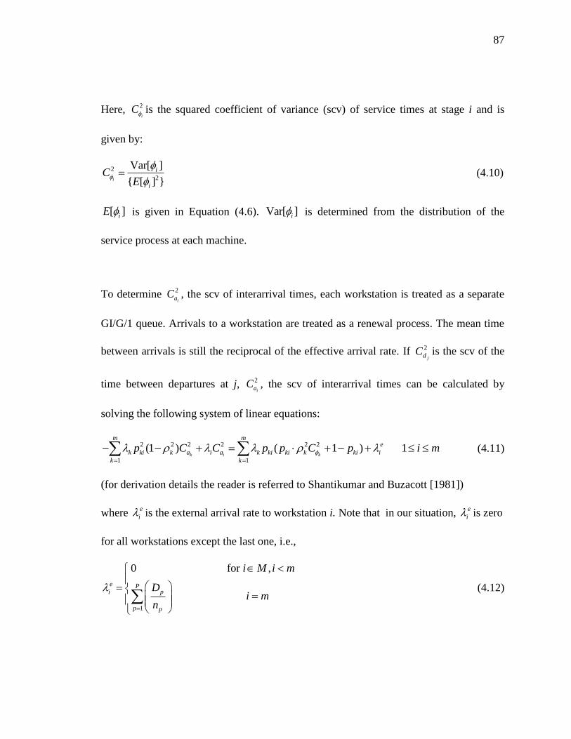
87
Here, 2
iC is the squared coefficient of variance (scv) of service times at stage i and is
given by:
2
2
Var[ ]
{ [ ] }i
i
i
CE
(4.10)
[ ]iE is given in Equation (4.6). Var[ ]i is determined from the distribution of the
service process at each machine.
To determine 2
iaC , the scv of interarrival times, each workstation is treated as a separate
GI/G/1 queue. Arrivals to a workstation are treated as a renewal process. The mean time
between arrivals is still the reciprocal of the effective arrival rate. If 2
jdC is the scv of the
time between departures at j, 2
iaC , the scv of interarrival times can be calculated by
solving the following system of linear equations:
2 2 2 2 2 2
1 1
(1 ) ( 1 ) 1k i k
m me
k ki k a i a k ki ki k ki i
k k
p C C p p C p i m
(4.11)
(for derivation details the reader is referred to Shantikumar and Buzacott [1981])
where e
i is the external arrival rate to workstation i. Note that in our situation, e
i is zero
for all workstations except the last one, i.e.,
1
0 for ,
e Ppi
p p
i M i m
Di m
n
(4.12)
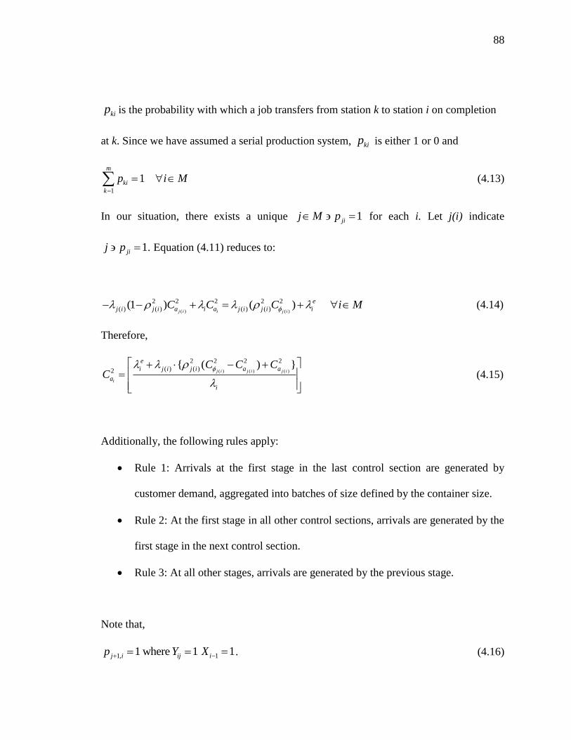
88
kip is the probability with which a job transfers from station k to station i on completion
at k. Since we have assumed a serial production system, kip is either 1 or 0 and
1
1m
ki
k
p i M
(4.13)
In our situation, there exists a unique 1jij M p for each i. Let j(i) indicate
1jij p . Equation (4.11) reduces to:
( ) ( )
2 2 2 2 2
( ) ( ) ( ) ( )(1 ) ( )j i i j i
e
j i j i a i a j i j i iC C C i M (4.14)
Therefore,
( ) ( ) ( )
2 2 2 2
( ) ( )2{ ( ) }
j i j i j i
i
e
i j i j i a a
a
i
C C CC
(4.15)
Additionally, the following rules apply:
Rule 1: Arrivals at the first stage in the last control section are generated by
customer demand, aggregated into batches of size defined by the container size.
Rule 2: At the first stage in all other control sections, arrivals are generated by the
first stage in the next control section.
Rule 3: At all other stages, arrivals are generated by the previous stage.
Note that,
1, 1 where 1j i ijp Y 1 1iX . (4.16)

89
We summarize the flow relations as:
If 1 1iX then:
1, 1 for smallest index > and 1
0 otherwise
j i j
ji
p j i X
p
(4.17)
If 1 0iX then:
1, 1
0 -1
i i
ji
p
p j i
(4.18)
Consider a hypothetical case in a six-stage serial system where stages 4 and 6 are chosen
as control points. This situation is shown in Figure 4.1. Conceptually, in this system,
arrivals at stages 2, 3, and 6 are generated by stages 1, 2, and 5 respectively. Arrivals at
stage 1 are generated by stage 5 and arrivals at stage 5 are generated by end customer
demand.
1 5 3 2
Flow of material
Flow of information
i Workstation i
buffer
4 6
Figure 4.1: Hypothetical structure where stages 4 and 6 are control points
Therefore , if stage i is the first stage in the last control section (Case 1), then:
90
For deterministic arrivals,2 0iaC . Otherwise, for each part type, p,
2
iaC is the scv of an
entire container. Therefore, ,
2
i paC , the scv for each product at the first stage in the last CS,
can be calculated from the distribution of the sum of np end customer demands. For
exponential end customer demand arrivals, the distribution of the entire container is a
gamma random variable with a mean of (n/Dp) and a variance of (n/Dp2). Therefore:
,
2 1i pa
p
Cn
2
iaC is the weighted sum of the scv for each product:
12
1
/
i
P
p p
p
a P
p
p
D n
C
D
(4.19)
If stage i is the first stage in a control section and stage l is the first stage in the next
control section (Case 2), then:
2 2 2 2
2{ ( ) }
l l l
i
e
i l l a a
a
i
C C CC
(4.20)
If stage i is not the first stage in a control section (Case 3) then:
1 1 1
2 2 2 2
12{ ( ) }
i i i
i
e
i j i a a
a
i
C C CC
(4.21)
In order to combine Equations (4.19) through (4.21), we define a new variable, ij as
follows:
91
1 if stage is the first stage in control section
0 otherwiseib
i b
Then,
1 1 1
2 2 2 2
1 12
12 2 2 2
, 1
1
{ ( ) }(1 )
{ ( ) }
( ) 1 ,
i i i
i
l l l
e
i i i a a
a ib
i
me
i l b l l a a
l iib
i
C C CC
C C C
i m i b
(4.22)
To determine ib
Let bi represent the control section in which stage i is. bi is a function of the total number
of control points before stage i. For example, in Figure 1, b is 1 for stages 1, 2, and 3 and
2 for stages 4, 5, and 6.
( ) 1i j
j i
b X
(4.23)
The subscript i in Equation(4.23) indicates that b is calculated for each stage.
ib is therefore 1 if both, i and bi are 1 and zero otherwise. Therefore:
1
if 1
max{0, } otherwise
i
ib
i i
b i
b b
(4.24)

92
4.4 Determining the Control Points
Assuming that the container sizes for each product are known, the optimal set of control
points can be determined by solving the following problem:
1 1
1
1 1
( 1)
2
( )
P Pip p mp p
i i
i M i M p pp
P P
jp j ij ijp ip ip i
j M p i j i M p
a D h nMin f X
n
z h X Y h L t D
(4.25)
Subject to:
1ij
j i
Y i M
(4.26)
, ,ij jY X i j M i j (4.27)
1, ,ij i jY Y i j M (4.28)
1mX (4.29)
[0,1]jX j M (4.30)
[0,1] ,ijY i j M (4.31)
Here, the objective function, Equation (4.25), minimizes the sum of the total location
cost, setup cost, work-in-process (WIP) inventory holding cost and finished goods
inventory cost for partial containers, safety stock holding cost. The first term in the
objective function represents the fixed cost of locating a control point. The second term
represents the total period setup and material cost. The third term represents the WIP
93
inventory holding cost of the partial container available for final demand where we
assume units are consumed one at a time. The fourth term represents the safety stock
holding cost at each control point. Note that in evaluating the safety stock, we assume
that the number of kanbans is continuous. A more accurate technique of calculating the
number of kanbans is described in Section 5.1.1. The fifth term represents WIP inventory
cost for units flowing through the system.
Once again we will use the shortest path transformation for locating the control points.
Consider stage 0 to be the input stage. Also, let Moj be the cost of selecting stage j as the
first inventory control point and Mjk, the cost of having j and k as two consecutive control
points. Also define
1 if stages and are two consecutive control points
0 otherwiseij
i jx
The ijx ‟s can be thought of as arcs connecting successive control points. Then, the above
formulation ((4.25) to(4.31)) can be modified as a shortest path problem as shown in
Chapter 3 as:
ij ij
i M j M
Min M x
(4.32)
Subject to:
1 if 0
0 if 0 or where , , ,
1 if
ij km
k M
i
x x i m i j k M k i j
i m
j M
(4.33)
94
[0,1] ,ijx i j M (4.34)
If np is fixed, 1
1 1
( 1)
2
P Pip p mp p
i M p pp
a D h nk
n
, is a constant for all feasible solutions.
Thus, in order to find the optimal solution to the model, we can ignore these two terms
from the objective function. In general:
1 1,
1 1 1
( )k P P
jk k ip ip i p kp j kp
i j p p
M f h L t D z h
(4.35)
Theorem 1 can be modified for evaluating the shortest path model in this case.
Theorem 3: For the cost structure defined in Equation (4.35), a single control point is
always optimal, i.e., stage m is the only control point, if for all stages j,
1 1 1,
1
1 1 1
1 1 1 1 1 1
( ) ( ) ( )
P
j mp mp jp jp mp j mp
p
jm P P m P
ip p ip i ip p ip i ip p ip i
i p i p i j p
f z h h h
h D L t h D L t h D L t
.
Proof: The proof follows the same procedure used in Theorem 1.
95
4.5 Determining Container Sizes
The formulation in Section 4.4 assumes that the container sizes are known. The
formulation for determining the optimal container sizes remains the same, with additional
constraints:
max
p in n i M (4.36)
0 1...pn p P (4.37)
1i i M (4.38)
Equation (4.38) can be rewritten as:
1
( ) 1P
p
ip p ip
p p
DS n
n
(4.39)
The decision variables here are np, Xj, and Yij. We consider two cases here:
Case 1 – Equal container sizes: Every product has the same container size n.
The above formulation is modified to:
1
i M 1 1 1 1
( 1)Min ( )
2
P P P Pip p mp
ip ip i p jp j ij ijp
p i M p j M p i j p
a D h nh L t D z h X Y
n
(4.40)
Subject to:
1ij
j i
Y i M
(4.41)
, ,ij jY X i j M i j (4.42)

96
1, ,ij i jY Y i j M (4.43)
1mX (4.44)
[0,1]jX j M (4.45)
[0,1] ,ijY i j M (4.46)
max
in n i M (4.47)
0n (4.48)
1i i M (4.49)
Constraint (4.49) can be rewritten as:
1
1
(1 )
P
p ip
p
P
ip
p
D S
n
(4.50)
We can solve (4.40) as an unconstrained optimization problem. The optimal container
size is then (the derivation is similar to the single product one shown in Chapter 3):
1
'
'
1 1
2
( )
( )i
i
P
ip ip
i M popt
j
rp qP Pr i
ij ip ip p q
j M i j p i M pijp
a D
n
W
z Z h D W
(4.51)

97
Constraint (4.50) gives us a lower limit on the container size, nmin (1
min
1
(1 )
P
p ip
p
P
ip
p
D S
n
).
Therefore, the optimal container size, * max( , )opt
minn n n
where ' i
i
q
q
dWW
dn . Because the waiting time at a stage depends on its location in the
control section, it is convenient to calculate '
iqW numerically. Here,
2 2
1
1
2 2
1
1
( ) ( )( ) ( 1) ( )
21
( 1) ( 1) 1( ( 1))
21
1
i i
i i
i i
Pp
p
a p
q q ip pPp
p
p
Pp
p
a p
ip pPp
p
p
Dp
C n C n nW n W n S n
Dp
n
Dp
C n C n nS n
Dp
n
The solution procedures in this case are similar to the ones described in Section 3.1.4.
Note that when setup costs are zero, the optimal solution is to have the same n for all p
products. This is clear from the objective function(4.40). Here, the objective function is
minimized when each np is 1.
Case 2 – Product dependent container size: The container size once again does not vary
across sections but each product has a different container size. The optimal container
sizes can be determined by solving the formulation given in Equations (4.25) to (4.31)
and (4.36) (4.38). Due to the interaction between the different products, finding a closed
98
form is not as trivial as in Case 1 and the container sizes and the control structure can be
determined by solving the Mixed Integer Non-Linear Programming (MINLP) problem.
4.6 Computational Results
Experiments are conducted to answer the following questions:
Does the control structure differ for a stochastic model and a deterministic model?
Is the control structure dependent on the number of products? As the number of
products increases, does the number of control points decrease?
The experiment design is described in Section 4.6.1.
4.6.1 Experiment Design
The following parameters are used:
P = 1, 2, 5, and 20 (number of products)
Dp = D/p (Daily demand for each product) – we assume that every product has
the same demand rate.
End customer demand distribution = deterministic, exponential with rate D/p
Sip = 0 (Setup time in days for a container of parts)
t = 0, 0.5 (transportation time in days for a container of parts)
c = 0.1 (collection time in days for a kanban)
m = 6, 20 (total number of stages)
99
All products are assumed to have the same Uniform processing time
distribution per unit. To calculate the upper and lower bounds, utilization
factors of 60% and 90% are used. Utilization is the ratio of number of arrivals
of containers per day to the number containers of parts served during the day.
Therefore,
1 1
10.6 or 0.9
1/( )
P Pp p
i ip p ip
p pp ip p ip p
D DS D
n S n n
(4.52)
Since the setup time in our experiments is equal to zero at all stages and the
demand per product is known, the processing time per product can be easily
computed from the above equation.
Holding cost ratio: ratio of hm to h1 = 6 and 20
Value added structure: increase in h from stage 1 to stage m = linear and
delayed capitalization. Figure 4.2 plots the holding cost increase for the
delayed linear pattern and Figure 4.3 for the capitalization pattern.
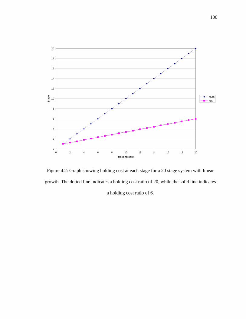
100
Figure 4.2: Graph showing holding cost at each stage for a 20 stage system with linear
growth. The dotted line indicates a holding cost ratio of 20, while the solid line indicates
a holding cost ratio of 6.
0
2
4
6
8
10
12
14
16
18
20
0 2 4 6 8 10 12 14 16 18 20
Holding cost
Sta
ge h(20)
h(6)
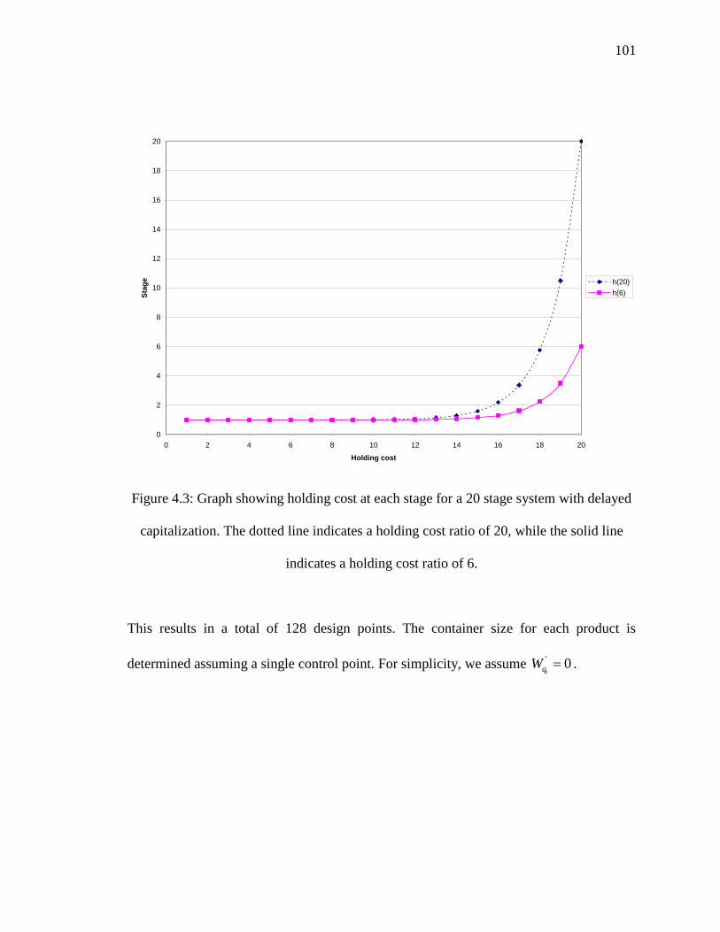
101
Figure 4.3: Graph showing holding cost at each stage for a 20 stage system with delayed
capitalization. The dotted line indicates a holding cost ratio of 20, while the solid line
indicates a holding cost ratio of 6.
This results in a total of 128 design points. The container size for each product is
determined assuming a single control point. For simplicity, we assume ' 0iqW .
0
2
4
6
8
10
12
14
16
18
20
0 2 4 6 8 10 12 14 16 18 20
Holding cost
Sta
ge
h(20)
h(6)

102
4.6.2 Discussion of Results
The effect of various factors on the system cost and control structure is discussed in this
Section.
4.6.2.1 Effect of factors on cost and control structure: Table 4.1 summarizes the results of
the experiments. Column A and B list the main effect of each factor on system cost and
the number of control points located respectively. Column C lists the total number of
solutions with multiple control points for each level while Column D lists the maximum
number of control points obtained for each factor level. A complete design table is
provided in Appendix 3.
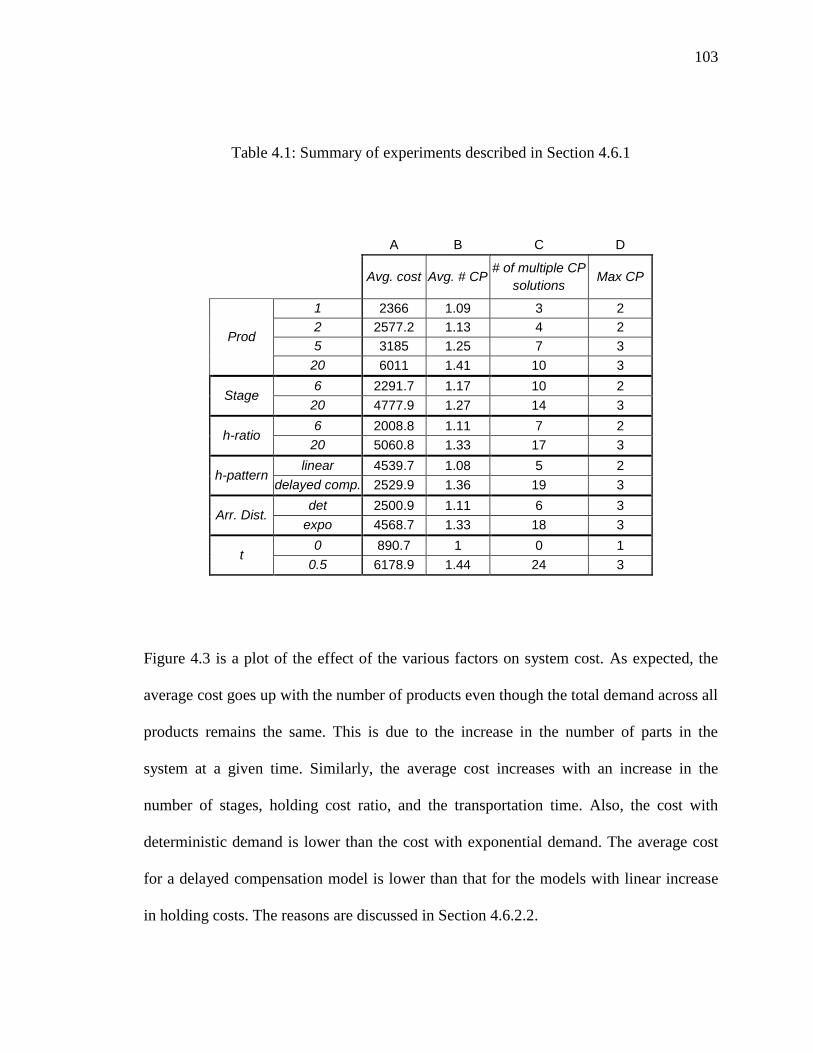
103
Table 4.1: Summary of experiments described in Section 4.6.1
A B C D
Avg. cost Avg. # CP
# of multiple CP
solutions Max CP
Prod
1 2366 1.09 3 2
2 2577.2 1.13 4 2
5 3185 1.25 7 3
20 6011 1.41 10 3
Stage 6 2291.7 1.17 10 2
20 4777.9 1.27 14 3
h-ratio 6 2008.8 1.11 7 2
20 5060.8 1.33 17 3
h-pattern linear 4539.7 1.08 5 2
delayed comp. 2529.9 1.36 19 3
Arr. Dist. det 2500.9 1.11 6 3
expo 4568.7 1.33 18 3
t 0 890.7 1 0 1
0.5 6178.9 1.44 24 3
Figure 4.3 is a plot of the effect of the various factors on system cost. As expected, the
average cost goes up with the number of products even though the total demand across all
products remains the same. This is due to the increase in the number of parts in the
system at a given time. Similarly, the average cost increases with an increase in the
number of stages, holding cost ratio, and the transportation time. Also, the cost with
deterministic demand is lower than the cost with exponential demand. The average cost
for a delayed compensation model is lower than that for the models with linear increase
in holding costs. The reasons are discussed in Section 4.6.2.2.
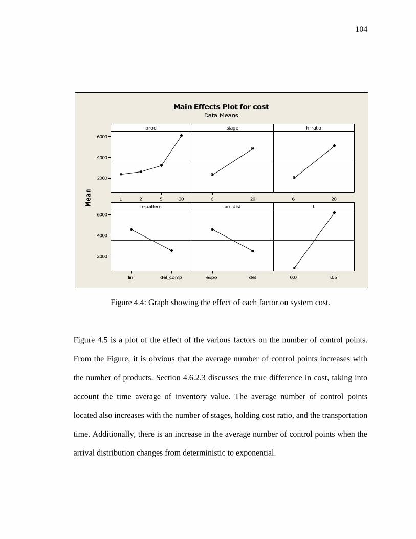
104
Figure 4.4: Graph showing the effect of each factor on system cost.
Figure 4.5 is a plot of the effect of the various factors on the number of control points.
From the Figure, it is obvious that the average number of control points increases with
the number of products. Section 4.6.2.3 discusses the true difference in cost, taking into
account the time average of inventory value. The average number of control points
located also increases with the number of stages, holding cost ratio, and the transportation
time. Additionally, there is an increase in the average number of control points when the
arrival distribution changes from deterministic to exponential.
20521
6000
4000
2000
206 206
del_complin
6000
4000
2000
detexpo 0.50.0
prod
Me
an
stage h-ratio
h-pattern arr dist t
Main Effects Plot for cost
Data Means

105
Figure 4.5: Graph showing the effect of each factor on system control structure.
4.6.2.2 Effect of holding cost distribution: The average number of control points
increases as we move from a linear increase in holding costs to a delayed differentiation
scenario. This is consistent with the observations for the single product model (see
Section 3.3.3). The average cost however goes down for a delayed differentiation model.
It is clear that in a delayed differentiation model, cost is reduced by locating more control
points at earlier stages where the holding costs are lower.
4.6.2.3 Effect of number of products: Since all products have the same set of control
points, an increase in the number of products obviously results in a corresponding
20521
1.4
1.3
1.2
1.1
1.0
206 206
del_complin
1.4
1.3
1.2
1.1
1.0
detexpo 0.50.0
prod
Me
an
stage h-ratio
h-pattern arr dist t
Main Effects Plot for num cpData Means

106
increase in the total holding cost at the control points. Figure 4.6 plots the effect of the
number of products on total cost for different values of the transportation time. From the
figure, it is clear that the total cost is directly related to the number of products held at
that stage and the lead time demand that is to be satisfied.
Therefore, having more control points not only decreases the number of parts held at each
control point but also reduces the transportation lead time that needs to be accounted for.
Figure 4.7, which plots the effect of the number of products on the ratio of total average
cost to the number of control points for different values of the transportation time shows
that the model tries to keep the ratio constant as the number of products increases. Figure
4.8 plots the combined effect of number of products and number of stages the system
control structure. It is clear from the figure that the average number of control points
increases consistently with an increase in the number of products, irrespective of the
number of stages in the manufacturing system.

107
Figure 4.6: Graph showing the combined effect of transportation time and number of
products on the average cost.
Effect of number of products on cost
1378.1
633.6 713.7 837.4
4098.4
4440.7 5532.6
10644
0
2000
4000
6000
8000
10000
12000
0 5 10 15 20
# of products
t=0.0
t=0.5
To
tal C
os
t

108
Figure 4.7: Graph showing the combined effect of transportation time and number of
products on the ratio of total cost to the number of control points.
0.50.0
7000
6000
5000
4000
3000
2000
1000
0
t
Me
an
1
2
5
20
prod
Interaction Plot for cost/cp
Data Means
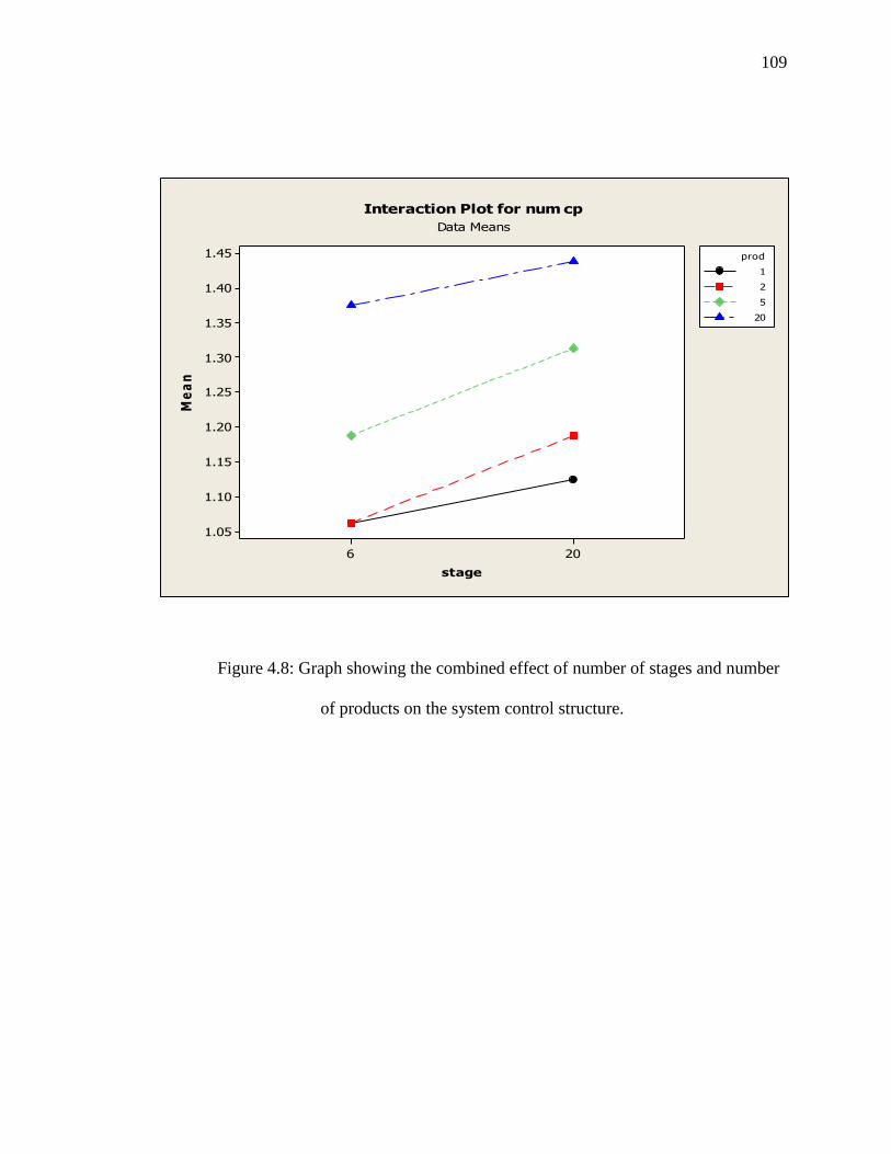
109
Figure 4.8: Graph showing the combined effect of number of stages and number
of products on the system control structure.
206
1.45
1.40
1.35
1.30
1.25
1.20
1.15
1.10
1.05
stage
Me
an
1
2
5
20
prod
Interaction Plot for num cp
Data Means

110
CHAPTER 5: MODEL VERIFICATION AND VALIDATION
A simulation model is built in Arena to verify the validity of our mathematical models. A
separate model is constructed for each control system architecture. We first discuss the
single part deterministic model. Additionally, comparative results for the models in
Chapters 3 and 4 with the simulation model will be presented.
5.1 Simulation Model logic
In this Section, the logic behind the simulation model is presented.
5.1.1 Determining the Number of Kanbans
We use the following equation to determine the number of kanbans in any control secti
on:
1 1* ( ) ( )j ij i i j j j ij i i
i j j M i j
j
D c Y L t z h X c Y L t
kn
(5.1)
The first term in the numerator of Equation (5.1) represents the total lead time demand,
and the second term represents the safety stock. Since each kanban authorizes the

111
production of one container of parts, the expression is normalized by the container size.
The number of kanbans in process at any time at the control section controlled by stage j
is determined using Little‟s law, p
j j ijk , where p
jk is the number of kanbans in
process, ij is the total processing time for a container of parts, and j is the arrival rate of
orders for containers. Here, i is the first stage in the control section controlled by stage j.
5.1.2 Creation of Orders
The logic for the single-part, single control point model will be discussed in this section.
Figure 5.1 shows the arrival of orders in the system. We model the arrival of containers
of parts, rather than individual parts in this simulation model. Since the demand for parts
is D units every day and each container n parts, this corresponds to the arrival of an order
for a container order every n/D days on an average. The orders enter an orders queue and
wait there until they receive a signal code of 231. The logic for this signal code is shown
in Figure 5.2 and is explained in Section 5.1.3.
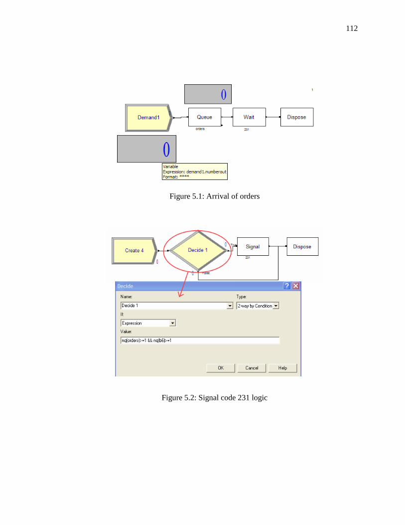
112
Figure 5.1: Arrival of orders
Figure 5.2: Signal code 231 logic

113
5.1.3 Simulation Logic
An entity is created every 0.01 days (to ensure that this even occurs more often than the
arrival and service events, thus ensuring more accurate wait times) and it checks to see if
there are containers parts waiting in the output queue of workstation 6 and in the orders
queue. If so, a signal code of 231 is generated. This signal results in the removal of a
single container of part from the output queue of machine 6 and one order from the orders
queue. Once a container of parts is removed from the output queue of workstation 6, the
number of kanbans at workstation 6 is incremented by after c days. Note that in our
model the kanban is modeled as a variable, rather than an entity for simplicity. Figure 5.3
shows the workstations. The logic is discussed in the following Section.

114
Figure 5.3: Workstations
5.1.4 Creation of Entities Corresponding to Containers of Parts and Workstation Logic
The number of kanbans at each control section is first calculated as described in Section
5.1.1. Each kanban corresponds to a container of parts. Initially, at time zero, k6
containers of parts are introduced at stage 1 in a single control section environment and at
the first stage of each control section in an environment with multiple control sections.
For each entity that enters into the system, the number of kanbans at stage 6 is
decremented by one. This corresponds to the removal of a kanban from the schedule
board and placing it into a container. Entities that finish processing at one workstation are
either transported to the next workstation (for entities coming out of workstations 1

115
through 5) or they are sent to the output queue at workstation 6. At the output queue,
these entities wait for signal code 231 (discussed in Section 5.1.3). Once an entity gets a
signal, it is duplicated. One of these duplicate entities is sent to an input queue (thus
keeping the WIP in the system constant) where it waits for a signal 123, while the other
increments the number of kanbans by one after a delay corresponding to the collection
time, after which it is disposed. Figure 5.4 shows the logic for signal code 123. An entity
is created every 0.01 days, which checks to see if there are any kanbans in the schedule
board. If there is, a container of parts (one entity) is released into the system.

116
Figure 5.4: Logic for signal code: 123
The cost expression is:
66
6 6
1
6 6
1 1
( -1)( ( ) / ) ( )
2
( ( . ) . + ( . )
i
i
i i i i i
i i
h nf a D n h nq b n
n h nq wss Queue WIP wss h WIP trans
(5.2)
where,
( . )inq wss Queue corresponds to the average number of entities in the input queue for
workstation i.
6( )nq b is the average number of parts in the output queue at workstation 6.
WIP.wssi represents the average WIP inventory at workstation i.
WIP.transi is the average number of containers in the transporter between workstation i
and i+1.
The first term in Equation (5.2) corresponds to the fixed location cost. The second term
corresponds to the setup cost. The third term represents the WIP inventory holding cost
of the partial container available for final demand where we assume units are consumed
one at a time. These three terms are the same as the first three terms in Equation (3.2).

117
The fourth term represents the safety stock holding cost, the fifth term, the WIP holding
cost and the last term, the holding cost during transportation.
Seven workstations are defined in the resources, six representing the six workstations,
and the seventh representing the transportation system (with infinite capacity). The
simulation model is verified by comparing it to a hand simulation model.

118
5.2 Model Validation
In this Section, experiments to validate both the Simulation model and the Mathematical
models described in earlier chapters are described. Note that the simulation model is
allowed to run for twenty three days with one replication (with a startup period of three
days) for the deterministic models and one hundred and fifty days, with 20 replications
(with a startup period of 20 days) for the stochastic models. Costs are averaged to find the
average daily cost.
5.2.1 Methods to Ensure That Both Models Are Equivalent
The mathematical model assumes a real number of kanbans while calculating the safety
stock inventory, whereas the simulation model rounds it up the next highest integer. The
following two methods are provided to ensure consistency between the simulation model
and the mathematical model:
computing mathematical model costs with integer number of kanbans (as
described in Section 5.1.1).
running simulation model with increased container collection time to reflect
partial container. Thus: ( )new
nc c k k
D
.
For our models, we use the first technique.
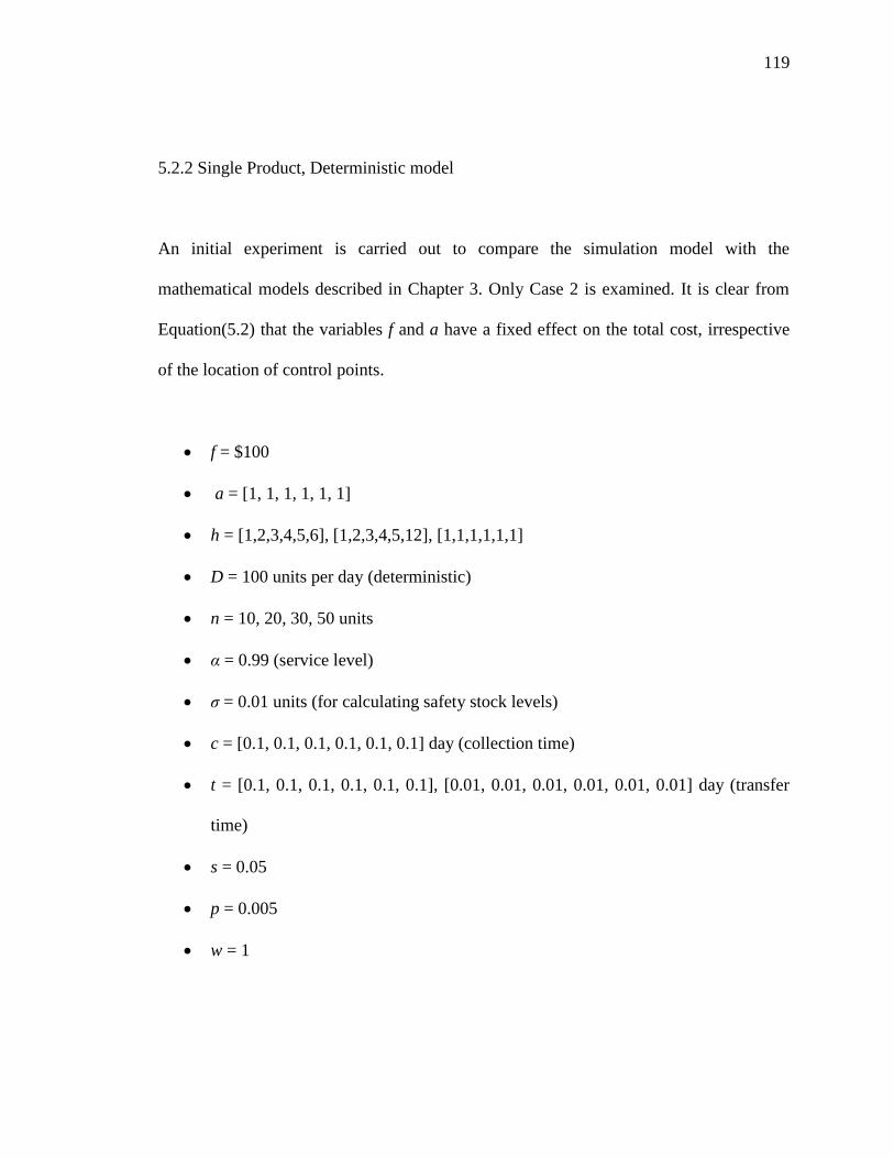
119
5.2.2 Single Product, Deterministic model
An initial experiment is carried out to compare the simulation model with the
mathematical models described in Chapter 3. Only Case 2 is examined. It is clear from
Equation(5.2) that the variables f and a have a fixed effect on the total cost, irrespective
of the location of control points.
f = $100
a = [1, 1, 1, 1, 1, 1]
h = [1,2,3,4,5,6], [1,2,3,4,5,12], [1,1,1,1,1,1]
D = 100 units per day (deterministic)
n = 10, 20, 30, 50 units
α = 0.99 (service level)
σ = 0.01 units (for calculating safety stock levels)
c = [0.1, 0.1, 0.1, 0.1, 0.1, 0.1] day (collection time)
t = [0.1, 0.1, 0.1, 0.1, 0.1, 0.1], [0.01, 0.01, 0.01, 0.01, 0.01, 0.01] day (transfer
time)
s = 0.05
p = 0.005
w = 1

120
The results of the simulation model are compared with a hand simulation for validation.
The results of the experiment are shown in Table 5.1. The total WIP holding cost during
production and transportation, Safety stock holding cost, and the total cost are compared
for the simulation model and the mathematical model for different design configurations.
In order to ensure a level playing field, the number of kanbans is rounded up to the
nearest integer in calculating safety stocks for the mathematical model. It is clear that in
general, the simulation model and the mathematical model follow the same pattern and
the cost components are almost identical for both models. The average cost difference
between the two models, 32
1
( )0.018.r r
r r
SC OC
SC
Here, SCr is the simulation cost for
design run r, while OCr is the mathematical model cost for design run r.
It is also to be noted that both the simulation model and mathematical model behave in a
similar manner to changes in the container size. Additionally, it is noted that when a two
control point solution is optimal for the mathematical model, the simulation cost for a
single control point solution is higher than that for a two-control-point solution (not
indicated in Table 5.1).
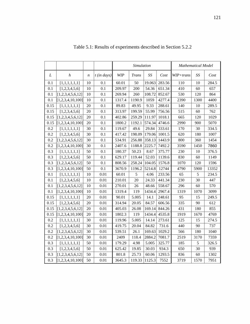
121
Table 5.1: Results of experiments described in Section 5.2.2
Simulation Mathematical Model
L h n t (in days) WIP Trans SS Cost WIP+trans SS Cost
0.1 [1,1,1,1,1,1] 10 0.1 60.01 50 19.063 283.56 110 10 284.5
0.1 [1,2,3,4,5,6] 10 0.1 209.97 200 54.36 651.34 410 60 657
0.1 [1,2,3,4,5,6,12] 10 0.1 269.94 260 108.72 852.67 530 120 864
0.1 [1,2,3,4,10,100] 10 0.1 1317.4 1190.9 1059 4277.4 2390 1300 4400
0.15 [1,1,1,1,1,1] 20 0.1 89.83 49.95 9.33 288.61 140 10 289.5
0.15 [1,2,3,4,5,6] 20 0.1 313.97 199.59 55.99 756.56 515 60 762
0.15 [1,2,3,4,5,6,12] 20 0.1 402.86 259.29 111.97 1018.1 665 120 1029
0.15 [1,2,3,4,10,100] 20 0.1 1800.2 1192.1 574.34 4746.6 2990 900 5070
0.2 [1,1,1,1,1,1] 30 0.1 119.67 49.6 29.84 333.61 170 30 334.5
0.2 [1,2,3,4,5,6] 30 0.1 417.42 198.09 179.06 1001.5 620 180 1007
0.2 [1,2,3,4,5,6,12] 30 0.1 534.91 256.88 358.13 1443.9 800 360 1454
0.2 [1,2,3,4,10,100] 30 0.1 2407.6 1188.8 2225.7 7492.2 3590 1450 7860
0.3 [1,1,1,1,1,1] 50 0.1 180.37 50.23 8.67 375.77 230 10 376.5
0.3 [1,2,3,4,5,6] 50 0.1 629.17 119.44 52.03 1139.6 830 60 1149
0.3 [1,2,3,4,5,6,12] 50 0.1 808.56 258.24 104.05 1576.8 1070 120 1596
0.3 [1,2,3,4,10,100] 50 0.1 3670.9 1196.2 5214.8 12744 4790 5900 13352
0.1 [1,1,1,1,1,1] 10 0.01 60.01 5 4.06 233.56 65 5 234.5
0.1 [1,2,3,4,5,6] 10 0.01 210.01 20 24.33 441.34 230 30 447
0.1 [1,2,3,4,5,6,12] 10 0.01 270.01 26 48.66 558.67 296 60 570
0.1 [1,2,3,4,10,100] 10 0.01 1319.4 119 1434.4 2967.4 1319 1070 3099
0.15 [1,1,1,1,1,1] 20 0.01 90.01 5.005 14.1 248.61 95 15 249.5
0.15 [1,2,3,4,5,6] 20 0.01 314.94 20.05 84.57 606.56 335 90 612
0.15 [1,2,3,4,5,6,12] 20 0.01 405.03 26.08 169.14 844.26 431 180 855
0.15 [1,2,3,4,10,100] 20 0.01 1802.3 119 1434.4 4535.8 1919 1670 4769
0.2 [1,1,1,1,1,1] 30 0.01 119.96 5.005 14.14 273.61 125 15 274.5
0.2 [1,2,3,4,5,6] 30 0.01 419.75 20.04 84.82 731.6 440 90 737
0.2 [1,2,3,4,5,6,12] 30 0.01 539.51 26.1 169.63 1029.2 566 180 1040
0.2 [1,2,3,4,10,100] 30 0.01 2409 118.4 2884.2 7081.7 2519 3170 7359
0.3 [1,1,1,1,1,1] 50 0.01 179.29 4.98 5.005 325.77 185 5 326.5
0.3 [1,2,3,4,5,6] 50 0.01 625.42 19.85 30.03 934.3 650 30 939
0.3 [1,2,3,4,5,6,12] 50 0.01 801.8 25.73 60.06 1293.5 836 60 1302
0.3 [1,2,3,4,10,100] 50 0.01 3645.3 119.33 1125.3 7552 3719 1570 7951
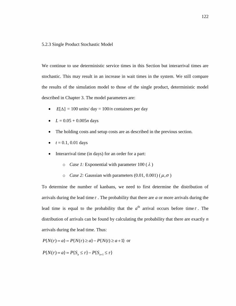
122
5.2.3 Single Product Stochastic Model
We continue to use deterministic service times in this Section but interarrival times are
stochastic. This may result in an increase in wait times in the system. We still compare
the results of the simulation model to those of the single product, deterministic model
described in Chapter 3. The model parameters are:
[ ]E = 100 units/ day = 100/n containers per day
L = 0.05 + 0.005n days
The holding costs and setup costs are as described in the previous section.
t = 0.1, 0.01 days
Interarrival time (in days) for an order for a part:
o Case 1: Exponential with parameter 100 ( )
o Case 2: Gaussian with parameters (0.01, 0.001) ( , )
To determine the number of kanbans, we need to first determine the distribution of
arrivals during the lead time . The probability that there are a or more arrivals during the
lead time is equal to the probability that the ath
arrival occurs before time . The
distribution of arrivals can be found by calculating the probability that there are exactly n
arrivals during the lead time. Thus:
{ ( ) } { ( ) } { ( ) 1}P N a P N a P N t a or
1{ ( ) } { } { }a aP N a P S P S

123
When the interarrival time between orders for individual parts is exponential with
parameter , the number of orders that arrive during a given time is given by a
Poisson distribution with a rate of . Therefore the number of parts that arrive
during the lead time is given by and has a variance of too.
When the interarrival time between orders for individual parts is Normal ( , ) ,
the number of arrivals during a day is empirically determined by generating 1000
inter-arrival times and analyzing the distribution of number of arrivals during a
given time period. The distribution for daily arrivals is approximately with a mean
of 10 and a standard deviation of 1. (Note that this is in tune with the predictions
of the Central Limit Theorem for renewal processes, which states that the limiting
distribution of number of arrivals is approximately Normal.)
The simulation model lumps orders together into containers. Therefore, for Case 1, with
exponential inter-arrival times between orders for individual parts the arrival of orders for
a container of parts follows a Gamma distribution with parameters 1/ and n. For Case
2, the distribution is Normal with a mean of n and a variance of 2n . Table 5.2
contains the results of the model for Case 1 while Table 5.3 contains the results for Case
2. It is clear from the Table that even with a high variance in the arrival distribution; the
deterministic mathematical model is reasonably accurate. The average cost difference
between the two models, 32
1
( )0.38r r
r r
SC OC
SC
with Exponential demand and 0.55 with
Normal demand. Again, SCr is the simulation cost for design run r, while OCr is the
optimization model cost for design run r. The 95% confidence interval for the simulation
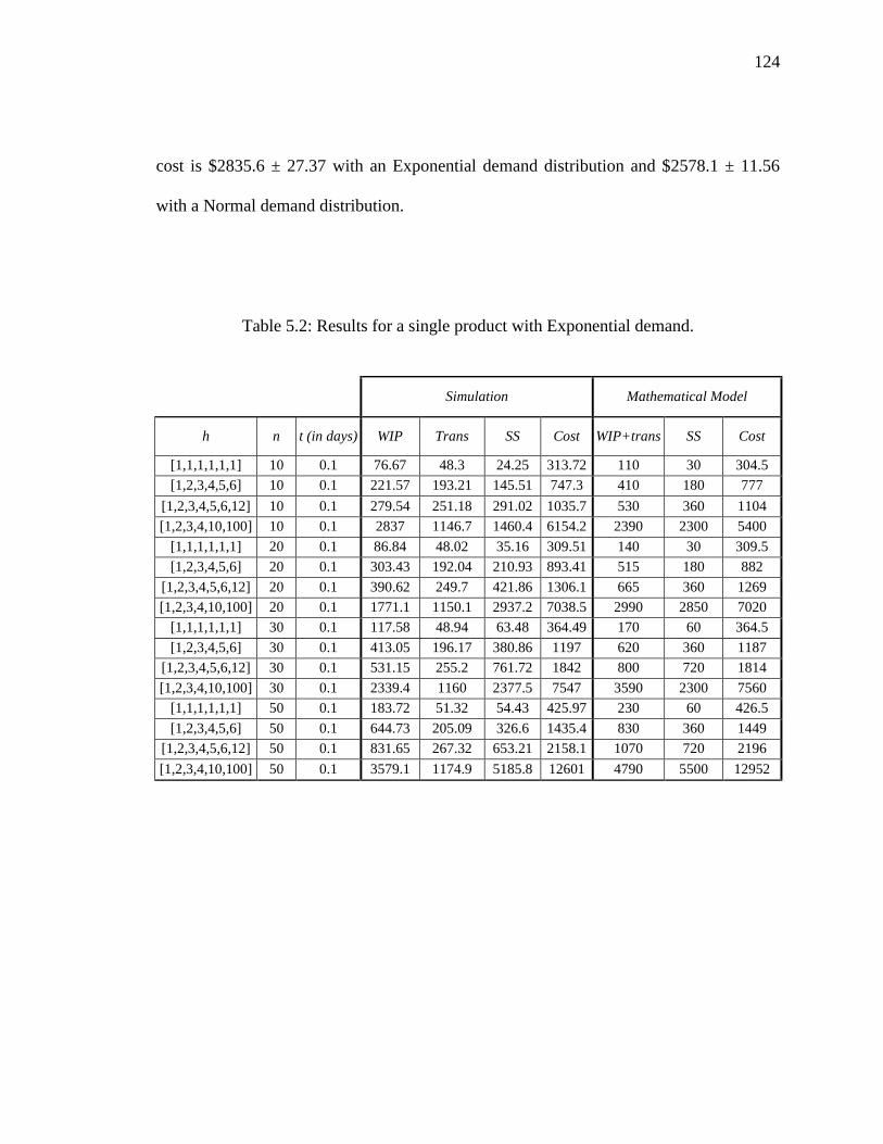
124
cost is $2835.6 ± 27.37 with an Exponential demand distribution and $2578.1 ± 11.56
with a Normal demand distribution.
Table 5.2: Results for a single product with Exponential demand.
Simulation Mathematical Model
h n t (in days) WIP Trans SS Cost WIP+trans SS Cost
[1,1,1,1,1,1] 10 0.1 76.67 48.3 24.25 313.72 110 30 304.5
[1,2,3,4,5,6] 10 0.1 221.57 193.21 145.51 747.3 410 180 777
[1,2,3,4,5,6,12] 10 0.1 279.54 251.18 291.02 1035.7 530 360 1104
[1,2,3,4,10,100] 10 0.1 2837 1146.7 1460.4 6154.2 2390 2300 5400
[1,1,1,1,1,1] 20 0.1 86.84 48.02 35.16 309.51 140 30 309.5
[1,2,3,4,5,6] 20 0.1 303.43 192.04 210.93 893.41 515 180 882
[1,2,3,4,5,6,12] 20 0.1 390.62 249.7 421.86 1306.1 665 360 1269
[1,2,3,4,10,100] 20 0.1 1771.1 1150.1 2937.2 7038.5 2990 2850 7020
[1,1,1,1,1,1] 30 0.1 117.58 48.94 63.48 364.49 170 60 364.5
[1,2,3,4,5,6] 30 0.1 413.05 196.17 380.86 1197 620 360 1187
[1,2,3,4,5,6,12] 30 0.1 531.15 255.2 761.72 1842 800 720 1814
[1,2,3,4,10,100] 30 0.1 2339.4 1160 2377.5 7547 3590 2300 7560
[1,1,1,1,1,1] 50 0.1 183.72 51.32 54.43 425.97 230 60 426.5
[1,2,3,4,5,6] 50 0.1 644.73 205.09 326.6 1435.4 830 360 1449
[1,2,3,4,5,6,12] 50 0.1 831.65 267.32 653.21 2158.1 1070 720 2196
[1,2,3,4,10,100] 50 0.1 3579.1 1174.9 5185.8 12601 4790 5500 12952
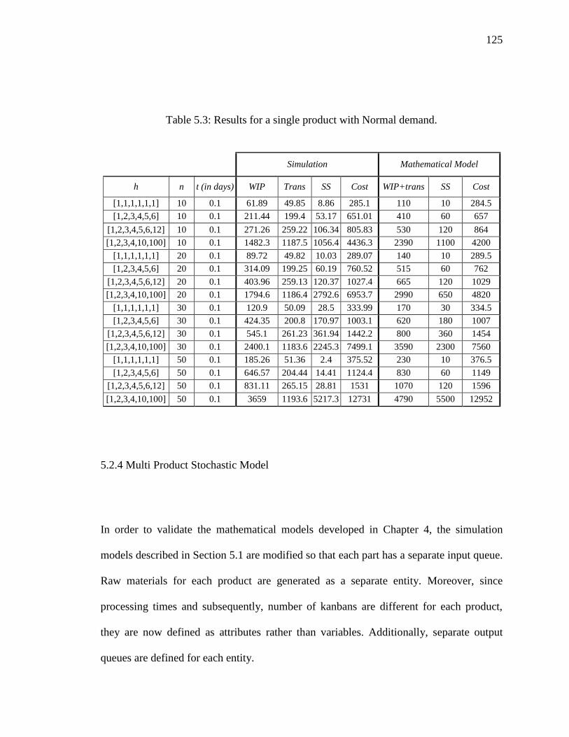
125
Table 5.3: Results for a single product with Normal demand.
Simulation Mathematical Model
h n t (in days) WIP Trans SS Cost WIP+trans SS Cost
[1,1,1,1,1,1] 10 0.1 61.89 49.85 8.86 285.1 110 10 284.5
[1,2,3,4,5,6] 10 0.1 211.44 199.4 53.17 651.01 410 60 657
[1,2,3,4,5,6,12] 10 0.1 271.26 259.22 106.34 805.83 530 120 864
[1,2,3,4,10,100] 10 0.1 1482.3 1187.5 1056.4 4436.3 2390 1100 4200
[1,1,1,1,1,1] 20 0.1 89.72 49.82 10.03 289.07 140 10 289.5
[1,2,3,4,5,6] 20 0.1 314.09 199.25 60.19 760.52 515 60 762
[1,2,3,4,5,6,12] 20 0.1 403.96 259.13 120.37 1027.4 665 120 1029
[1,2,3,4,10,100] 20 0.1 1794.6 1186.4 2792.6 6953.7 2990 650 4820
[1,1,1,1,1,1] 30 0.1 120.9 50.09 28.5 333.99 170 30 334.5
[1,2,3,4,5,6] 30 0.1 424.35 200.8 170.97 1003.1 620 180 1007
[1,2,3,4,5,6,12] 30 0.1 545.1 261.23 361.94 1442.2 800 360 1454
[1,2,3,4,10,100] 30 0.1 2400.1 1183.6 2245.3 7499.1 3590 2300 7560
[1,1,1,1,1,1] 50 0.1 185.26 51.36 2.4 375.52 230 10 376.5
[1,2,3,4,5,6] 50 0.1 646.57 204.44 14.41 1124.4 830 60 1149
[1,2,3,4,5,6,12] 50 0.1 831.11 265.15 28.81 1531 1070 120 1596
[1,2,3,4,10,100] 50 0.1 3659 1193.6 5217.3 12731 4790 5500 12952
5.2.4 Multi Product Stochastic Model
In order to validate the mathematical models developed in Chapter 4, the simulation
models described in Section 5.1 are modified so that each part has a separate input queue.
Raw materials for each product are generated as a separate entity. Moreover, since
processing times and subsequently, number of kanbans are different for each product,
they are now defined as attributes rather than variables. Additionally, separate output
queues are defined for each entity.

126
The parameters used and the results are shown below:
p = 2 products
f = $100
a = [1, 1, 1, 1, 1, 1] for both products
h = [1,2,3,4,5,6] for both products
α = 0.99 (service level)
σ = 0.01 units (for calculating safety stock levels)
c = [0.1, 0.1, 0.1, 0.1, 0.1, 0.1] day (collection time)
t = [0.1, 0.1, 0.1, 0.1, 0.1, 0.1] day (transfer time)
s = 0.05
p = Discrete[0.004, 0.006] (indicating that the processing time at a machine is
either 0.004 days or 0.006 days)
w = 1
n = 15
End customer demand for each product is Exponential with a rate of 50 units per day.
Table 5.4 contains the results of the experiments. The waiting times at each of the six
stages, safety stock cost, WIP and transportation cost and the total cost are listed for each
model. For example, for a container size of 10, the waiting time at the first stage obtained
with the simulation model (Sim) is 0.03691 days, while the waiting time predicted by the
mathematical model (Math) is 0.02553. Similarly, for the second stage, the simulation

127
model gives a waiting time of 0.00912 days while the mathematical model predicts a
waiting time of 0.01399 days.
Table 5.4: Results of experiments described in Section 5.2.4
Cost Sim Math
n=10
Waiting times
0.03691, 0.00912,
0.01103, 0.01217,
0.01319, 0.01395
0.02533, 0.01399,
0.01052, 0.009466,
0.009143, 0.00904
SS 314.43 484.77
WIP+Trans 315.64+197.02 403.52
Total 1009.1 1053.64
n=20
Waiting times
0.08173, 0.00777,
0.00778, 0.00793,
0.00792, 0.00792
0.04525, 0.0112,
0.0094, 0.0086,
0.0083, 0.0081
SS 535.19 534.02
WIP+Trans 293.11 + 165.75 383.55
Total 1176 1137
n=30
Waiting times
0.03689, 0.01622,
0.01869, 0.02199,
0.02602, 0.02852
0.01112, 0.01021,
0.0097, 0.00937,
0.00901, 0.00912
SS 442.75 639.88
WIP+Trans 526.7 + 201.4 504.8
Total 1377.8 1324.16
There is clearly a difference in the waiting times predicted by the mathematical model
and the waiting times given by the simulation model, especially for higher container
sizes. In order to verify if this difference is due to a difference in the squared coefficient
of variation of arrivals, we run another experiment with the following parameters:

128
σ = 0.01 units (for calculating safety stock levels)
c = [0.001, 0.001, 0.001, 0.001, 0.001, 0.001] day (collection time)
t = [0.001, 0.001, 0.001, 0.001, 0.001, 0.001] day (transfer time)
s = 0.004
p = Discrete[0.001, 0.009]
n = 1
The squared coefficient of variation of arrivals and the waiting times at each of the six
stages obtained with the simulation model are:
Simulation:
Ca2 = 0.79, 0.3028, 0.261, 0.26, 0.25, 0.24
Waiting times: 0.03966, 0.02421, 0.01967, 0.02265, 0.02583, 0.02369
The values predicted by the mathematical model are:
Mathematical Model
Ca2 = 1, 0.35, 0.2265, 0.2031, 0.199 , 0.198
Waiting times: 0.0485, 0.02218, 0.01717, 0.01623, 0.01604, 0.01601
It is clear that the squared coefficients of variance are almost alike for the simulation and
mathematical model and the simulation model. The difference in the waiting times can
therefore be attributed to the fact that the formula used for calculating waiting times at
machines are simply approximations.
129
CHAPTER 6: SUMMARY AND CONCLUSIONS
In this dissertation, we have shown that under reasonable conditions on inventory holding
costs, and a predetermined container size, a pull system should combine stages into a
single control sector and use a single output buffer. However, multiple buffers may be
preferable if lead times are significant and the value added between stages is significant.
Choice of container size and minimum production batch can be incorporated into the
model.
Chapter 3 models a single product production system with deterministic arrival and
service times. The shortest path model describes or serves as a useful subproblem for
several extensions of the basic formulation. Although we consider only a single-product
scenario here, the results and theorems in this chapter are valid in a multi-product case if
every product visits the same set of workstations.
Chapter 4 incorporates the stochastic effect of workstation variability, multiple products
and structures, and queuing effects. A similar methodology to the one used in Chapter 3
is used for determining the optimal buffer location. The effect of arrival distribution,
number of products, value added structure, and transit times for containers of parts on the
total system cost and the system control structure is investigated.
130
Finally, in Chapter 5, a simulation model is presented in order to validate the models in
Chapters 3 and 4.

131
APPENDIX A: CODE
Model to determine the optimal continer sizes and optimal control structure for a single-
product, deterministic model:
#include "mainfun.h"
//Global variables
int numstage; //number of stages
int F; //Fixed cost of locating an IC pt
float c; //collection time
float t; //transfer time
float sigma; //std. dev. of daily demand
double z; //std. normal variate
double p; //processing time per unit
double s; //setup time
int D; //Daily demand
double alpha; //service level
int pathlen; //number of nodes on shortest path
double *A;
double *h;
int *nmax;
double old_n; //value of n from previous iteration
vector <vector <double> > M; //cost vector
//int **M;
vector <int> chosen; //stages on shortest path
int n; //batch size
int nupper; // upper bound on n
double batch; //min of max allowable batch sizes
ofstream fout; // for file writing
//Function to calculate batch sizes
double f(double n, double b){
double sumA=0;
double sumH=0;
for(int iter_j=0;iter_j<numstage;iter_j++){
sumA+=A[iter_j+1];
sumH+=h[iter_j+1];
}
double numer = 2*D*sumA; //numerator
//Denominator

132
int temp=pathlen-1;
double den=0;
while (temp>0){
double p_sum=0;
double tau_sum=0;
for(int iter_j=chosen[temp]+1;iter_j<=chosen[temp-
1];iter_j++){
p_sum=p_sum+p;
tau_sum = tau_sum + ( s + p*n) + t;
}
den+=(min(h,numstage)*p_sum/sqrt(c+tau_sum));
//cout<<"den is :\n"<<den;
temp--;
}
den+=h[numstage]+(2*D*sumH*p);
double fract = sqrt(numer/den);
/*
cout<<"\n the value of n: "<<n;
cout<<"\n the value of numer: "<<numer;
cout<<"\n the value of den: "<<den;*/
return(abs(n-fract));
}//end function
//Function to determine n
double golden_search(double b){
double X=0;
double t=0.618034;
double a=0; //lower bound on batch size
double epsilon=0.00001; // Precision
double lambk=a + ((1-t)*(b-a));
double muk=a + t*(b-a);
double fxr=f(lambk,b);
double fxl=f(muk,b);
while((b-a)>epsilon){
if(fxr>fxl){
a=lambk;
lambk=muk;
fxr=fxl;
muk=a+t*(b-a);
fxl=f(muk,b);
}
else{
b=muk;
muk=lambk;

133
fxl=fxr;
lambk=a+(1-t)*(b-a);
fxr=f(lambk,b);
}
}
return((b+a)/2);
}// end function golden
//Function to calculate cost matrix
void cost_cal(int n){
//int **M; //cost matrix
/*M = new int * [numstage+1];
for(int iter_i = 0; iter_i < numstage+1; iter_i ++)
M[iter_i] = new int [numstage+1];*/
M.resize(numstage+1);
for(int iter_i=0;iter_i<=numstage;iter_i++)
M[iter_i].resize(numstage+1);
double A1;
double L1;
double hL;
double nmin=1000;
double sumh;
for(int iter_j= 0;iter_j<numstage;iter_j++){
for(int iter_k=iter_j+1;iter_k<=numstage;iter_k++){
A1=0;
L1=0;
hL=0;
nmin=1000;
sumh=0;
double L=(s+p*n);
for(int iter_l = iter_j+1;iter_l<=iter_k;iter_l++){
// cout<<iter_l;
A1=A1+A[iter_l];
L1=L1+L;
hL=hL+(h[iter_l]*L*D)+(h[iter_l]*D*t);
//hL+=1;
//cout<<"ldkjfksj "<<L;
sumh=sumh+h[iter_l];
}
M[iter_j][iter_k]= (double)F+ (double)(A1*D/n)+
(double)(floor((double)(iter_k/numstage)))*(h[iter_k]*(n-1)/2)+
(double)(hL)+(double)(z*sigma*h[iter_k]*sqrt(L1 + c + (double)(iter_k-
iter_j)*t));
}
}

134
for(int iter_k = 0;iter_k<=numstage;iter_k++){
M[numstage][iter_k]=0;
}
}// end cost_cal
//Use Djikstra's algorithm to find the shortest path
void djikstra(){
chosen.erase(chosen.begin(),chosen.end());//Erase vector
pathlen=0; //set pathlen back to zero
double *label;
label =new double[numstage+1];
label[0]=0;
double epsilon=0.05;
for(int iter_i=1;iter_i<=numstage;iter_i++)
label[iter_i]=100000000; //initially set label to a very
high value
for(int iter_j = 0;iter_j<numstage;iter_j++){
for(int iter_k=iter_j+1;iter_k<=numstage;iter_k++){
label[iter_k] =
min(label[iter_k],label[iter_j]+M[iter_j][iter_k]);
}
}
/*cout<<"dji\n";
for(int temp=0;temp<numstage;temp++)
cout<<label[temp]<<"\t";*/
//chosen.resize(1);
chosen.push_back(numstage);
//pathlen++;//increment pathlen, since an element has been added
to chosen
int j=numstage;
while ( j>0){
int path=1;
for(int k=j-1;k>=0;k--){
//cout<<"Djikstra"<<"\n";
//cout<<"\n";
//cout<<k<<"\t"<<abs(label[j]-M[k][j]-label[k]);
if(abs(label[j]-M[k][j]-label[k])<epsilon){
path++;
chosen.push_back(k);
j=k;
}
}
}
pathlen = (int)chosen.size();
cout<<"CHOSEN\n";

135
for(int temp=0;temp<pathlen;temp++)
cout<<chosen[temp]<<"\t";
cout<<"\n";
}//end djikstra
//MAIN FUNCTION
int main(int argc, char * argv[]){
// X. Need filename
if (argc < 2)
{
cerr << "Usage: " << argv[0] << " filename.txt\n";
exit(1);
}
ifstream fin;
fin.open(argv[1]);
if (!fin.is_open())
{
cerr << "\nCouldn't open file " << argv[1] << " ... Abort";
fin.clear(); // reset failbit
return false;
}
cout<<endl;
fin>>numstage;
A= new double[numstage+1];//Setup cost
h = new double[numstage+1]; //holding cost matrix
vector <double> L(numstage+1); //lead time
nmax = new int[numstage+1]; //max allowable batch size
fin>>F;
for(int iter_i=0;iter_i<=numstage;iter_i++) fin>>A[iter_i];
for(int iter_i=0;iter_i<=numstage;iter_i++) fin>>h[iter_i];
fin >>c;
fin>>t;
fin>>D;
fin>>sigma;
for(int iter_i=0;iter_i<=numstage;iter_i++) fin>>nmax[iter_i];
fin>>alpha;
fin>>z;
fin>>p;
fin>>s;
// Time calculation variables
time_t wallclock_start;
time_t wallclock_stop;
double wallclock;
cout << endl << "********* PROCEDURE BEGIN ********* " << endl;
wallclock_start = clock();
/*
136
//Print values for verifications
cout<<"\nnumstage\t"<<numstage;
cout<<"\nF\t"<<F;
cout<<"\nA\t";
for(int iter_i=0;iter_i<=numstage;iter_i++)
cout<<A[iter_i]<<"\t";
cout<<"\nh\t";
for(int iter_i=0;iter_i<=numstage;iter_i++)
cout<<h[iter_i]<<"\t";
cout<<"\nc\t"<<c;
cout<<"\nt\t"<<t;
cout<<"\nD\t"<<D;
cout<<"\nsigma\t"<<sigma;
cout<<"\nnmax\t";
for(int iter_i=0;iter_i<=numstage;iter_i++)
cout<<nmax[iter_i]<<"\t";
cout<<"\nalpha\t"<<alpha;
cout<<"\nz\t"<<z;
cout<<"\np\t"<<p;
cout<<"\ns\t"<<s;
*/
//Initially, to calculate batch size, assume a single control
point
//int chosen[] ={numstage,0}; //nodes on the shortest path
//chosen.resize(2);
chosen.push_back(numstage);
chosen.push_back(0);
pathlen=(int)chosen.size();
//Calculate the smallest of the max batch sizes
batch=10000;
for(int iter_i=1;iter_i<=numstage;iter_i++){
if (nmax[iter_i]<batch) batch=nmax[iter_i];
}
nupper = (int)ceil(golden_search(batch)); //Upper bound on n
n=1;
//define mincost to be the minimum total cost
double Totcost; //total cost for each n value
double mincost=10000000; //set mincost to a big number
int opt_n=1; //n that gives the minimum cost
vector <int> opt_chosen; //stages on optimal path
//cout<<"\n\n"<<n;
while(n<=nupper){
cost_cal(n);
djikstra();
Totcost = 0;
for(int temp= pathlen-1;temp>=1;temp--){
Totcost=Totcost + M[chosen[temp]][chosen[temp-1]];
}
if(Totcost<=mincost){
mincost=Totcost;

137
opt_n = n;
opt_chosen = chosen;
}
n++;
}
n--;
//open file results.txt for writing (append).
for(int iter_i=0;iter_i<=numstage;iter_i++){
for(int iter_j=0;iter_j<=numstage;iter_j++){
cout<<M[iter_i][iter_j]<<" ";
}
cout<<endl;
}
fout.open("C:\\results22.xls",ofstream::app);
if(!fout.is_open()){
cerr<<"\n couldn't open file"<<" results22.xls"<<" to
write....program aborted";
fout.clear(); //reset failbit
return false;
}
else{
cout<<"Opened file for writing"<<endl;
}
wallclock_stop = clock();
wallclock = (double) (wallclock_stop - wallclock_start) /
CLOCKS_PER_SEC;
cout << "\nTotal wallclock time (in seconds) = " << wallclock <<
endl;
cout << "********* PROCEDURE END *********" << endl;
vector <int> chosen1;
chosen1=opt_chosen;
vector<int>::iterator endIterator;
endIterator = chosen1.end()-1;
chosen1.erase(endIterator);
fout<<endl;
print(mincost);
print(opt_n);
print(chosen1);
fout<<"\t";
print((int)chosen1.size());
fout.close();
cout<<"Total cost is: "<<mincost;
cout<<"\nOptimal batch size: "<<opt_n;
delete [] A,h,nmax;
A=NULL;
h=NULL;
nmax=NULL;
138
chosen.clear();
}//end main
void print(double d1){
fout<<d1<<"\t";
}
void print(int d1){
fout<<d1<<"\t";
}
void print(vector <int> &v1){
int temp=(int)v1.size();
for(int iter_i=0;iter_i<temp;iter_i++){
fout<<v1[iter_i]<<" ";
}
}
double min(double *array, int size){
double mini = 100000;
for(int i=0;i<numstage;i++){
if(array[i]<=mini) mini = array[i];
}
return(mini);
}
Multi-product, stochastic model (known container size)
//stochastic multiproduct case
#include "mainfun.h"
//Global variables
char dist[20];
int numstage; //number of stages
int F; //Fixed cost of locating an IC pt
float c; //collection time
float t; //transfer time
int p; //number of products
//Per product type variables
double *n; //batch size
double *sigma; //std. dev. of end customer demand for each product
double z; //std. normal variate
double **theta; //processing time per unit
double *s; //setup time
double *D; //Daily demand
double **A; //Setup + mat. handling cost
double **h; //Holding cost
//End of per product type variables
double cstara; //scv of arrivals
double cstars; //scv of service
double alpha; //service level
int pathlen; //number of nodes on shortest path
139
double tmax; //maximum container processing time
double old_n; //value of n from previous iteration
vector <vector <double> > M; //cost vector
//int **M;
vector <int> chosen; //stages on shortest path
int nupper; // upper bound on n
double batch; //min of max allowable batch sizes
ofstream fout; // for file writing
//Function to calculate batch sizes
void f(){
//double *temp;
//temp=new double[numstage+1];
//for(int iter_i=0;iter_i<p;iter_i++){
// for(int iter_j =0; iter_j<=numstage;iter_j++){
// temp[iter_j]= (tmax-s[iter_i])/theta[iter_i][iter_j];
// }
// n[iter_i]=min(temp,numstage+1);
// cout<<endl<<n[iter_i];
//}
// n[iter_i]=704
n[0]=4;
//n[1]=2;
}//end function
//Function to calculate cost matrix
void cost_cal(){
double **lambda; //Average arrival rate for each product at each
stage
double *lambda_i; //Avg. arrival rate at stage
double **mu; //service rate
double *ser; //expected service time
double *varser; //var. of service time
double *rho; //utilization
double *csq_s; //scv of service
double *csq_a; //scv of arrival
lambda = new double * [p];
for(int iter_i = 0; iter_i < p; iter_i ++)
lambda[iter_i] = new double [numstage+1];
mu = new double * [p];
for(int iter_i = 0; iter_i < p; iter_i ++)
mu[iter_i] = new double [numstage+1];
vector <vector <double> > L; //lead time
L.resize(p);
for(int iter_i=0;iter_i<p;iter_i++) L[iter_i].resize(numstage+1);

140
//Calculation of lead time (without waiting time)
for(int iter_j= 0;iter_j<p;iter_j++){
for(int iter_k=0;iter_k<=numstage;iter_k++){
L[iter_j][iter_k]=s[iter_j]+(n[iter_j]*theta[iter_j][iter_k]);
//
}
}
//Calculation of lambda[i][p] and mu[i][p]
for(int iter_j= 0;iter_j<p;iter_j++){
for(int iter_k=0;iter_k<=numstage;iter_k++){
if(iter_k==0){
lambda[iter_j][iter_k]=0;
mu[iter_j][iter_k]=0;
}
else{
lambda[iter_j][iter_k]=D[iter_j]/n[iter_j];
mu[iter_j][iter_k]=1/(L[iter_j][iter_k]);
}
}
}
lambda_i = new double [numstage+1];
//Calculation of lamdba[i]
for(int iter_k= 0;iter_k<=numstage;iter_k++){
lambda_i[iter_k]=0;
for(int iter_j=0;iter_j<p;iter_j++){
lambda_i[iter_k]+=lambda[iter_j][iter_k];
}
}
//Calculation of expected service time and rho
ser=new double[numstage+1];
rho = new double[numstage+1];
for(int iter_k= 0;iter_k<=numstage;iter_k++){
ser[iter_k]=0;
rho[iter_k]=0;
for(int iter_j=0;iter_j<p;iter_j++){
ser[iter_k]+=(lambda[iter_j][iter_k]/mu[iter_j][iter_k]);
}
if(iter_k==0){
rho[iter_k]=0;
ser[iter_k]=0;
}
else{
rho[iter_k]=ser[iter_k];
ser[iter_k]=ser[iter_k]/lambda_i[iter_k];
}
}
//Calculation of variance of service time
varser=new double[numstage+1];
for(int iter_k= 0;iter_k<=numstage;iter_k++){
141
varser[iter_k]=0;
for(int iter_j=0;iter_j<p;iter_j++){
double temp=(1/mu[iter_j][iter_k])-ser[iter_k];
varser[iter_k]+=lambda[iter_j][iter_k]*sqr(temp);
}
if(iter_k==0) varser[iter_k]=0;
else varser[iter_k]=varser[iter_k]/lambda_i[iter_k];
}
//Calculation of C-square(si)
csq_s = new double[numstage+1];
for(int iter_k= 0;iter_k<=numstage;iter_k++){
csq_s[iter_k]=varser[iter_k]/sqr(ser[iter_k]);
}
M.resize(numstage+1);
for(int iter_i=0;iter_i<=numstage;iter_i++)
M[iter_i].resize(numstage+1);
double A1;
double *L1;
double hL;
double nmin=1000;
double sumh;
L1= new double(p);
csq_a=new double[numstage+1];
double *W;
W=new double[numstage+1];
vector <vector <double> > L2; //actual lead time
L2.resize(p);
for(int iter_i=0;iter_i<p;iter_i++)
L2[iter_i].resize(numstage+1);
csq_a[0]=0;
W[0]=0;
//Cost Calculations (waiting time at station is also calculated
here)
//Note that the lead time, L calculated earlier does not include
the waiting time
//for(int iter_j= 0;iter_j<numstage;iter_j++){
// for(int iter_k=iter_j+1;iter_k<=numstage;iter_k++){
for(int iter_k= numstage;iter_k>=1;iter_k--){
for(int iter_j=0;iter_j<iter_k;iter_j++){
//cout<<iter_k;
A1=0;
for (int iter_t=0;iter_t<p;iter_t++) L1[iter_t]=0;
hL=0;
sumh=0;
double ss = 0;

142
for(int iter_l = iter_j+1;iter_l<=iter_k;iter_l++){
if(iter_l==iter_j+1){
//ASSUMPTION**************************************
if(iter_k==numstage){
if(strcmp(dist,"none")==0)csq_a[iter_l]=0.0; //for now
else if(strcmp(dist,"expo")==0){
double temp =0;
csq_a[iter_l]=0;
for(int
iter_m=0;iter_m<p;iter_m++){
csq_a[iter_l]+=D[iter_m]/n[iter_m];
temp+=D[iter_m];
}
csq_a[iter_l]=csq_a[iter_l]/temp;
//csq_a[iter_l]=0.1;
//cout<<dist<<"
"<<csq_a[iter_l]<<" "<<iter_l<<endl;
}
}//end if
else{
csq_a[iter_l]=max(0.0,(lambda_i[iter_l]+lambda_i[iter_k+1]*(sqr(r
ho[iter_k+1]) * (sqr(csq_s[iter_k+1])-sqr(csq_a[iter_k+1]))
+sqr(csq_a[iter_k+1])))/lambda_i[iter_l]);
}//end else if
}//end if iter_l==iter_j+1
else{
csq_a[iter_l]=max(0.0,(lambda_i[iter_l-
1]*(sqr(rho[iter_l-1]) *(sqr(csq_s[iter_l-1])-sqr(csq_a[iter_l-
1]))+sqr(csq_a[iter_l-1])))/lambda_i[iter_l]);
//cout<<"kjhskjs "<<iter_l-1<<"
"<<iter_k<<" "<<csq_a[iter_l-1]<<endl;
//csq_a[iter_l]=0;
}//end else if
if(iter_l==0) W[iter_l]=0;
else
W[iter_l]=max(0.0,sqr(rho[iter_l])*(1+sqr(csq_s[iter_l]))/(1+sqr(
rho[iter_l]*csq_s[iter_l]))*(sqr(csq_a[iter_l])+sqr(rho[iter_l]*csq_s[i
ter_l]))/2*lambda_i[iter_l]*(1-rho[iter_l]));
//W[iter_l]=sqr(rho[iter_l])*(1+sqr(csq_s[iter_l]))/(1+sqr(rho[it
er_l]*csq_s[iter_l]))*(sqr(csq_a[iter_l])+sqr(rho[iter_l]*csq_s[iter_l]
))/2*lambda_i[iter_l]*(1-rho[iter_l]);
for(int iter_m=0;iter_m<p;iter_m++){
W[iter_l]=0;

143
L2[iter_m][iter_l]=L[iter_m][iter_l]+W[iter_l];
cout<<"dfj "<<iter_l<<"
"<<W[iter_l]<<"\n";
}
L1[iter_m]=0;
//hL=0;
for(int iter_m=0;iter_m<p;iter_m++){
// cout<<iter_l;
A1=A1+(A[iter_m][iter_l]*D[iter_m]/n[iter_m]);
L1[iter_m]=L1[iter_m]+L2[iter_m][iter_l];
hL=hL+(h[iter_m][iter_l]*L2[iter_m][iter_l]*D[iter_m])+(h[iter_m]
[iter_l]*D[iter_m]*t);
//hL+=1;
//cout<<"dfj
"<<L[iter_m][iter_l]<<"\n";
//sumh=sumh+h[iter_l];
}
if(iter_l==numstage){
for(int iter_m=0;iter_m<p;iter_m++){
sumh= sumh+
(h[iter_m][iter_l]*(n[iter_m]-1));
}
}
//cout<<iter_k;
}
//cout<<iter_l;
for(int iter_m=0;iter_m<p;iter_m++){
if (strcmp(dist, "expo")==0) sigma[iter_m] =
D[iter_m];
ss+=(z*sigma[iter_m]*h[iter_m][iter_k]*sqrt(L1[iter_m] + c +
(double)(iter_k-iter_j)*t));
//cout<<L1[iter_m]<<" ";
cout<<"dfsdf "<<sigma[iter_m];
}
//ss=0.0;
//hL=0.0;
M[iter_j][iter_k]= (double)F+ (double)(A1)+
(double)(floor((double)(iter_k/numstage)))*(sumh/2)+
(double)(hL)+(double)ss;
// cout<<iter_l;
}

144
}
//for(int iter_k = 0;iter_k<=numstage;iter_k++){
//M[numstage][iter_k]=0;
//}
cout<<endl;
for(int iter_i=0;iter_i<=numstage;iter_i++){
for(int iter_j=0;iter_j<=numstage;iter_j++){
cout<<M[iter_i][iter_j]<<" ";
}
cout<<endl;
}
//for(int iter_i=0;iter_i<=numstage;iter_i++)
// cout<<csq_a[iter_i]<<" ";
// cout<<endl;
}// end cost_cal
//Use Djikstra's algorithm to find the shortest path
void djikstra(){
chosen.erase(chosen.begin(),chosen.end());//Erase vector
pathlen=0; //set pathlen back to zero
double *label;
label =new double[numstage+1];
label[0]=0;
double epsilon=0.05;
for(int iter_i=1;iter_i<=numstage;iter_i++)
label[iter_i]=100000000; //initially set label to a very
high value
for(int iter_j = 0;iter_j<numstage;iter_j++){
for(int iter_k=iter_j+1;iter_k<=numstage;iter_k++){
label[iter_k] =
min(label[iter_k],label[iter_j]+M[iter_j][iter_k]);
}
}
chosen.push_back(numstage);
int j=numstage;
while ( j>0){
int path=1;
for(int k=j-1;k>=0;k--){
if(abs(label[j]-M[k][j]-label[k])<epsilon){
path++;
chosen.push_back(k);
j=k;
}

145
}
}
pathlen = (int)chosen.size();
cout<<"CHOSEN\n";
for(int temp=0;temp<pathlen;temp++)
cout<<chosen[temp]<<"\t";
cout<<"\n";
}//end djikstra
//MAIN FUNCTION
int main(int argc, char * argv[]){
// X. Need filename
//If no file name is specified:
if (argc < 2)
{
cerr << "Usage: " << argv[0] << " filename.txt\n";
exit(1);
}
ifstream fin;
fin.open(argv[1]);
if (!fin.is_open())
{
cerr << "\nCouldn't open file " << argv[1] << " ... Abort";
fin.clear(); // reset failbit
return false;
}
cout<<endl;
fin.getline(dist, sizeof(dist), '\n');
fin>>numstage;
fin >>p;
//VARIABLE DECLARATION
D=new double[p]; //demand
A = new double * [p];//Setup cost
for(int iter_i = 0; iter_i < p; iter_i ++)
A[iter_i] = new double [numstage+1];
h = new double * [p];//holding cost matrix
for(int iter_i = 0; iter_i < p; iter_i ++)
h[iter_i] = new double [numstage+1];
theta = new double * [p];//processing time matrix
for(int iter_i = 0; iter_i < p; iter_i ++)
theta[iter_i] = new double [numstage+1];
//lambda = new double[p];
sigma = new double[p];
s=new double[p];

146
//theta = new double[p];
//nmax = new int[p]; //max allowable batch size
//END VARIABLE DECLARATION - START TAKING VALUES
fin>>F;
for(int iter_i=0;iter_i<p;iter_i++) {
for(int iter_j=0;iter_j<=numstage;iter_j++)
fin>>A[iter_i][iter_j];
}
for(int iter_i=0;iter_i<p;iter_i++) {
for(int iter_j=0;iter_j<=numstage;iter_j++)
fin>>h[iter_i][iter_j];
}
for(int iter_i=0;iter_i<p;iter_i++) {
for(int iter_j=0;iter_j<=numstage;iter_j++)
fin>>theta[iter_i][iter_j];
}
for(int iter_i=0;iter_i<p;iter_i++)
fin>>D[iter_i];
for(int iter_i=0;iter_i<p;iter_i++)
fin>>sigma[iter_i];
for(int iter_i=0;iter_i<p;iter_i++)
fin>>s[iter_i];
//for(int iter_i=0;iter_i<p;iter_i++)
// fin>>theta[iter_i];
//for(int iter_i=0;iter_i<p;iter_i++)
// fin>>lambda[iter_i];
//for(int iter_i=0;iter_i<p;iter_i++)
// fin>>nmax[iter_i];
fin>>tmax;
fin >>c;
fin>>t;
fin>>z;
fin>>cstara;
fin>>cstars;
fin>>alpha;
// Time calculation variables
time_t wallclock_start;
time_t wallclock_stop;
double wallclock;
cout << endl << "********* PROCEDURE BEGIN ********* " << endl;
wallclock_start = clock();
//Print values for verifications
cout<<dist<<endl;
cout<<"\nnumstage\t"<<numstage;
cout<<"\np\t"<<p;
cout<<"\nF\t"<<F;

147
cout<<"\nA\n";
for(int iter_i=0;iter_i<p;iter_i++) {
//cout<<iter_i<<endl;
for(int iter_j=0;iter_j<=numstage;iter_j++){
cout<<A[iter_i][iter_j]<<"\t";}
cout<<endl;
}
cout<<"\nh\n";
for(int iter_i=0;iter_i<p;iter_i++) {
for(int iter_j=0;iter_j<=numstage;iter_j++){
cout<<h[iter_i][iter_j]<<"\t";}
cout<<endl;
}
cout<<"\ntheta\n";
for(int iter_i=0;iter_i<p;iter_i++) {
for(int iter_j=0;iter_j<=numstage;iter_j++){
cout<<theta[iter_i][iter_j]<<"\t";}
cout<<endl;
}
cout<<"\nD\n";
for(int iter_i=0;iter_i<p;iter_i++) cout<<D[iter_i]<<"\t";
cout<<"\nsigma\n";
for(int iter_i=0;iter_i<p;iter_i++) cout<<sigma[iter_i]<<"\t";
cout<<"\ns\n";
for(int iter_i=0;iter_i<p;iter_i++) cout<<s[iter_i]<<"\t";
//cout<<"\ntheta\n";
//for(int iter_i=0;iter_i<p;iter_i++) cout<<theta[iter_i]<<"\t";
//cout<<"\nlambda\n";
//for(int iter_i=0;iter_i<p;iter_i++) cout<<lambda[iter_i]<<"\t";
cout<<"\ntmax\n"<<tmax;
cout<<"\nc\t"<<c;
cout<<"\nt\t"<<t;
cout<<"\nz\t"<<z;
cout<<"\nCstara\t"<<cstara;
cout<<"\nCstars\t"<<cstars;
cout<<"\nalpha\t"<<alpha;
cout<<endl<<"END"<<endl;
//Initially, to calculate batch size, assume a single control
point
//int chosen[] ={numstage,0}; //nodes on the shortest path
//chosen.resize(2);
chosen.push_back(numstage);
chosen.push_back(0);
pathlen=(int)chosen.size();
//define mincost to be the minimum total cost
double Totcost; //total cost for each n value
n=new double[p]; //set size of batch size array
vector <int> opt_chosen; //stages on optimal path
//cout<<"\n\n"<<n;
f();

148
cost_cal();
cout<<"END1";
djikstra();
Totcost = 0;
for(int temp= pathlen-1;temp>=1;temp--){
Totcost=Totcost + M[chosen[temp]][chosen[temp-1]];
}
//open file results.txt for writing (append).
fout.open("C:\\results22.xls",ofstream::app);
if(!fout.is_open()){
cerr<<"\n couldn't open file"<<" results22.xls"<<" to
write....program aborted";
fout.clear(); //reset failbit
return false;
}
else{
cout<<"Opened file for writing"<<endl;
}
wallclock_stop = clock();
wallclock = (double) (wallclock_stop - wallclock_start) /
CLOCKS_PER_SEC;
cout << "\nTotal wallclock time (in seconds) = " << wallclock <<
endl;
cout << "********* PROCEDURE END *********" << endl;
vector <int> chosen1;
chosen1=opt_chosen;
vector<int>::iterator endIterator;
endIterator = chosen1.end()-1;
chosen1.erase(endIterator);
fout<<endl;
print(Totcost);
print(*n);
print(chosen1);
fout<<"\t";
print((int)chosen1.size());
fout.close();
cout<<"Total cost is: "<<Totcost;
cout<<"\nOptimal batch size: "<<n[p-1];
delete [] A,h,tmax;
A=NULL;
h=NULL;
tmax=NULL;
chosen.clear();
}//end main
void print(double d1){
fout<<d1<<"\t";
}
149
void print(int d1){
fout<<d1<<"\t";
}
void print(vector <int> &v1){
int temp=(int)v1.size();
for(int iter_i=0;iter_i<temp;iter_i++){
fout<<v1[iter_i]<<" ";
}
}
void print (double* s){
for(int iter_i=0;iter_i<sizeof(s);iter_i++){
fout<<s[iter_i]<<" ";
}
}
double min(double *array, int size){
double mini = 100000;
for(int i=0;i<numstage;i++){
if(array[i]<=mini) mini = array[i];
}
return(mini);
}
//function to calculate square of a number
double sqr(double a){
return (a*a);
}
double max(double a, double b){
if(a>b) return(a);
else return(b);
}
150
APPENDIX B: DESIGN TABLE FOR EXPERIMENTS IN SECTION
4.6.2
The complete design table is shown in Tables A2.1 and A2.2. The first table shows the
effect of the factors on the number of control points located while the second table shows
their effect on the total system cost. The tables indicate the main effect of each factor as
well as the interactions between factors. For example, the cell corresponding to the row
with prod = 1 and the column with prod = 1 gives the number of control points located
(1.1) as well as the total cost ($2366) when the number of products is equal to 1.
Similarly, the cell corresponding to the row with prod = 1 and the column with stage = 6
gives the number of control points located (1.1) and the total cost ($3353.8).

151
Table A2.1 Effect of factors on number of control points
prod
stage
h_ratio
h-pattern
arr_dist
t
1 2 5 20 6 20 6 20 lin del_comp expo det 0 0.5
prod 1 1.1 - - - 1.1 1.1 1.1 1.1 1 1.2 1.2 1 1 1.2
2 - 1.1 - - 1.1 1.2 1.1 1.2 1 1.3 1.2 1.1 1 1.3
5 - - 1.3 1.2 1.3 1.1 1.4 1.1 1.4 1.4 1.1 1 1.5
20 - - - 1.4 1.4 1.4 1.2 1.6 1.2 1.6 1.5 1.3 1 1.8
stage 6 - - - - 1.2 - 1.1 1.3 1.1 1.3 1.3 1.1 1 1.3
20 - - - - - 1.3 1.2 1.4 1.1 1.5 1.4 1.2 1 1.5
h_ratio 6 - - - - - - 1.1 - 1 1.2 1.2 1 1 1.2
20 - - - - - - - 1.3 1.2 1.5 1.5 1.2 1.5 1.2
h_pattern lin - - - - - - - - 1.1 - 1.1 1 1 1.2
del_comp - - - - - - - - - 1.4 1.5 1.2 1 1.7
arr_dist expo - - - - - - - - - - 1.3 - 1 1.7
det - - - - - - - - - - - 1.4 1 1.2
t 0 - - - - - - - - - - - - 1 -
0.5 - - - - - - - - - - - - - 1.4
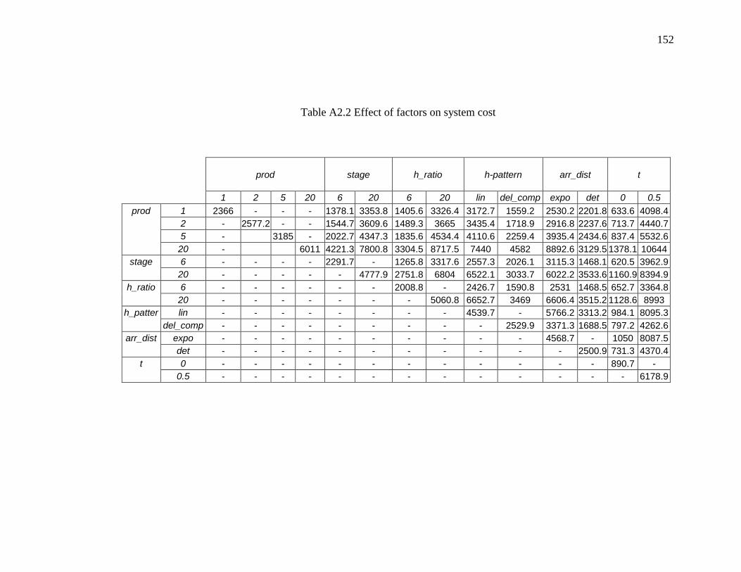
152
Table A2.2 Effect of factors on system cost
prod
stage
h_ratio
h-pattern
arr_dist
t
1 2 5 20 6 20 6 20 lin del_comp expo det 0 0.5
prod 1 2366 - - - 1378.1 3353.8 1405.6 3326.4 3172.7 1559.2 2530.2 2201.8 633.6 4098.4
2 - 2577.2 - - 1544.7 3609.6 1489.3 3665 3435.4 1718.9 2916.8 2237.6 713.7 4440.7
5 - 3185 - 2022.7 4347.3 1835.6 4534.4 4110.6 2259.4 3935.4 2434.6 837.4 5532.6
20 - 6011 4221.3 7800.8 3304.5 8717.5 7440 4582 8892.6 3129.5 1378.1 10644
stage 6 - - - - 2291.7 - 1265.8 3317.6 2557.3 2026.1 3115.3 1468.1 620.5 3962.9
20 - - - - - 4777.9 2751.8 6804 6522.1 3033.7 6022.2 3533.6 1160.9 8394.9
h_ratio 6 - - - - - - 2008.8 - 2426.7 1590.8 2531 1468.5 652.7 3364.8
20 - - - - - - - 5060.8 6652.7 3469 6606.4 3515.2 1128.6 8993
h_patter lin - - - - - - - - 4539.7 - 5766.2 3313.2 984.1 8095.3
del_comp - - - - - - - - - 2529.9 3371.3 1688.5 797.2 4262.6
arr_dist expo - - - - - - - - - - 4568.7 - 1050 8087.5
det - - - - - - - - - - - 2500.9 731.3 4370.4
t 0 - - - - - - - - - - - - 890.7 -
0.5 - - - - - - - - - - - - - 6178.9
153
REFERENCES
1. Afentakis, P., 1987, “A parallel heuristic algorithm for lot-sizing in multi-stage
production systems.” IIE Trans., 19, 34-42.
2. Afentakis, P., and B. Gavish, 1983, “Optimal lot-sizing algorithms for complex
product structures.” Oper. Res., 34(2), 237-249.
3. Afentakis, P., B. Gavish, and R.A. Millen, 1983, “Computationally efficient
optimal solutions to the lot-sizing problem in multistage assembly systems.”
Management Sci., 30, 222-239.
4. Askin, R. G., M. G. Mitwasi and J. B. Goldberg, 1993, “Determining the number
of kanbans in multi-item just-in-time systems.” IIE Transactions, 25(1), 89-98.
5. Askin, R. G. and J. W. Goldberg, 2002, “Design and analysis of lean production
systems.” Wiley, New York, NY.
6. Axsater, S., 1993, “Continuous review policies for multi-level inventory systems
with stochastic demand.” S. Graves, A. Rinooy Kan, and P. Zipkin (Eds.), in
Handbook in Operations Research and Management Science, Vol. 4, Logistics of
Production and Inventory. North Holland, 175-196.
7. Axsater, S., 1997, “Simple evaluation of echelon stock (R,Q) policies for two-
level inventory systems.” IIE Transactions, 29, 661-669.
8. Axsater, S. and K. Rosling, 1993, “Installation versus echelon inventory stocking
policies for multi-level inventory control.” Management Sci. 39(10), 1274-1280.
154
9. Axsater, S. and K. Rosling, 1994, “Multi level production-inventory control:
materials requirements planning or reorder point policies?” European Journal of
Operational Research, 75(2), 405-412.
10. Baker, K. R., 1993, “Requirements planning.” in S. C. Graves, A. Rinooy kan,
and P. Zipkin (Eds.), Logistics of Production and Inventory, North-Holland,
Amsterdam, 571-628.
11. Benton, W. C. and H. Shin, 1998, “Manufacturing planning and control: the
evolution of MRP and JIT integration.” European Journal of Oper. Res., 110,
411-440.
12. Berkeley, B. J., 1996, “A simulation study of container size in two card kanban
systems.” Int. J. Prod. Res., 34(12), 3417-3445.
13. Blackburn, J. D. and R.A. Millen, 1982, “Improved heuristics for multistage
requirements planning systems.” Management Sci., 28, 44-56.
14. Buzacott, J. A., and J. G. Shantikumar, 1994, “Safety stock versus safety time in
MRP controlled production systems.” Management Sci., 40(12), 1678-1689.
15. Buzacott, J. A. and J. G. Shantikumar, 1991, “The PAC system: a general
approach for coordinating multiple cell manufacturing systems.” Conference on
Multi-Echelon Inventory Systems, Berkeley, CA.
16. Cachon, G, 1995, “Exact evaluation of batch-ordering inventory policies in two-
echelon supply chains with periodic review.” Working paper, Duke University.

155
17. Cao, D. and M. Chen, 2005, “A mixed integer programming model for a two line
CONWIP-based production and assembly system.” International Journal of
Production Economics, 95, 317-326.
18. Chen, F, and Y.S. Zheng, 1994, “Evaluating echelon stock (R, nQ) policies in
serial production/ inventory systems with stochastic demand.” Management Sci.
40, 1262-1275.
19. Chen, F (2003), “Information Sharing and Supply Chain Coordination.” Ton G.
de Kok and Stephen C. Graves (Eds.) in Handbooks of Operations Research and
Management Science.
20. Chen, F., 1998, “Echelon reorder points, installation reorder points, and the value
of centralized demand information.” Management Sci. 44, pp. S221-S234.
21. Chen, F., 1999, “94%-effective policies for a two-stage serial inventory system
with stochastic demand.” Management Sci. 45, 1679-1696.
22. Chen, F., 2000, “Optimal policies for multi-echelon inventory problems with
batch ordering.” Oper. Res. 48, 376-389.
23. Chen, F., Z. Drezner, J.K. Ryan, and D. Simchi-Levi, 1998, “The Bullwhip
Effect: Managerial Insights on the Impact of Forecasting and Information on
Variability in a Supply Chain.” Sridhar Tayur, Ram Ganeshan and Michael
Magazine (Eds.) in Quantitative Models for Supply Chain Management. Boston:
Kluwer‟s International Series, 417-440.

156
24. Chen, F., Z. Drezner, J. Ryan, and D. Simchi-Levi, 2000a, “Quantifying the
Bullwhip Effect: the impact of Forecasting, Lead Times and Information.”
Management Science, 46, 436-443
25. Chen, F., Z. Drezner, J. Ryan, and D. Simchi-Levi, 2000b, “The Impact of
Exponential Smoothing Forecasts on the Bullwhip Effect.” Naval Research
Logistics, 47, 269-286.
26. Chen, F. and Y.S. Zheng, 1997, “One-warehouse, multi-retailer systems with
centralized stock information.” Oper. Res., 45(2), 275-287.
27. Chen, F. and Y.S. Zheng, 1998, “Near-optimal echelon-stock (R,nQ) policies in
multi-stage serial systems.” Oper. Res. 46, 592-602.
28. Chopra, S., and Meindl, P. (2001), “Supply chain management: Strategy, planning
and operation.” Upper Saddle River, NJ: Prentice-Hall.
29. Clark, A, and H. Scarf, 1960, “Optimal policies for a multi-echelon inventory
problem.” Management Sci., 6, 465-490.
30. Clark, A, and H. Scarf, 1962, “Approximate solutions to a simple multi-echelon
inventory problem.” Arrow, K. J. et al. (Ed.) in Studies in Applied Probability and
Management Science, Stanford University Press, CA, 88-100.
31. Crowston, W. B., Wagner, M., and Williams, J. F., 1973, “Economic lot size
determination in multi-stage assembly systems.” Management Sci., 19, 5, 517-
527.

157
32. Davis, W. J. and S. J. Stubitz, 1987, “Configuring a kanban system using a
discrete optimization of multiple stochastic responses.” Int. J. Prod. Res., 25, 721-
740.
33. De Bodt, M.A., and S.C. Graves, 1985, “Continuous review policies for multi-
echelon inventory problem with stochastic demand.” Management Sci. 31(10),
1286-1295.
34. Deleersnyder, J. L., T. J. Hodgson, H. Muller(-Malek) and P. J. Grady, 1989,
“Controlled pull systems: an analytic approach.” Management Sci., 35, 1079-
1091.
35. Dong, L., and H.L. Lee, 2003, “Optimal policies and approximations for a serial
multiechelon inventory system with time-correlated demand.” Oper. Res. 51, pp.
969-980.
36. Duenyas, I., W. J. Hopp, and M. L. Spearman. 1993, “Characterizing the output
process of a CONWIP line with determinisitic processing and random outages.”
Management Sci., 39(8), 975-988.
37. Duenyas, I. and W. J. Hopp, 1990, “Estimating variance of output from cyclical
exponential queueing systems.” Queueing Systems, 7, 337-354.
38. Federgruen, A., and P. Zipkin, 1984, “Computational issues in an infinite horizon,
multi-echelon inventory problem.” Oper. Res. 32, pp. 818-836.
39. Gavirneni, S, R. Kapuscinski, and S. Tayur, 1999, “Value of Information in
Capacitated Supply Chains.” Management Sci., 45, 16-24.
158
40. Golany, B., E.M. Dar-el, and N. Zeev, 1999, “Controlling shop floor operations in
a multi-family, multi-cell manufacturing environment through constant work-in-
process.” IIE Transactions, 31, 771-781.
41. Govil, M. K. and M.C. Fu, 1999, “Queueing Theory in manufacturing: a survey.”
Journal of Manufacturing Systems, 18(3), 214-240.
42. Grasso, E. T. and B.W. Taylor, 1984, “A simulation-based investigation of
supply/ timing uncertainty in MRP systems.” Int. J. Prod. Res., 22, 485-497.
43. Graves, S. C. and S.P. Willems, 2000,“Optimizing strategic safety stock
placement in supply chains.” Manufacturing & Service Oper. Mgmt., 2(1), 68-83.
44. Graves, S.C., 1996, “A multiechelon inventory model with fixed replenishment
intervals.” Management Sci. 42, 1-18.
45. Graves, S.C., and S.P. Willems, 2000, “Optimizing strategic safety stock
placement in supply chains.” Manufacturing and Oper. Management, 2, 68-83.
46. Gupta, Y. P. and M. C. Gupta, 1989a, “A system dynamics model of a JIT kanban
system.” Engr. Costs & Prod. Econ., 18, 117-130.
47. Gupta, Y. P. and M. C. Gupta, 1989b, “A system dynamics model for a multi-
stage dual-card JIT kanban system.” Engr. Costs & Prod. Econ., 18, 117-130.
48. Hahn, C. K., D.J. Bragg, and D. Shin, 1988, “Impact of the setup variable on
capacity and inventory decisions.” Academy of Mgmt. Review, 13(1), 91-103.

159
49. Herer, Y. T. and M. Masin, 1997, “Mathematical programming formulation of
CONWIP-based production lines; and relationships to MRP.” Int. J. Prod. Res.,
35(4), 1067-1076.
50. Hopp, W. J., and M. L. Roof, 1998, “Setting WIP levels with statistical
throughput control (STC) in CONWIP production lines; and relationships to
MRP.” Int. J. Prod. Res., 36(4), 867-882.
51. Hopp, W. J. and Spearmann, M. L. 1996, “Factory Physics: Foundations of
Manufacturing Management.” Irwin, Chicago, IL
52. Huang, C. and A. Kusiak, 1996, “Overview of kanban systems.” Int. J. Computer
Integrated Manufacturing, 9(3), 169-189.
53. Inderfuth, K., 1991, “Safety stock optimization in multi-stage inventory systems.”
Int. J. Prod. Econ., 24, 103-113.
54. Inderfuth, K., 1994, “Safety stocks in multistage divergent inventory systems: a
survey.” Int. J. of Prod. Econ, 35, 321-329.
55. Inderfuth, K. and S. Minner, 1998, “Safety stocks in multi-stage inventory
systems under different service measures.” European Journal of Oper. Res., 106,
57-73.
56. Karmarkar, U. S., S. Kekre, and S. Kekre, 1985, “Lot sizing in multi-item, multi-
machine job shops.” IIE Transactions, 17, 290-298.
57. Karmarkar, U. S. and S. Kekre, 1989, “Batching policy in kanban systems.”
Journal of Manuf. Sys., 8, 317-328.
160
58. Karmarkar, U.S., 1987, “Lot sizes, lead times and in-process inventories.” Mgmt.
Sci. 33(3), 409-418.
59. Krishnamurthy, A., R. Suri, and M. Vernon, 2004, “Re-examining the
performance of MRP and kanban material control policies for multi-product
flexible manufacturing systems.” The International Journal of Flexible
Manufacturing Systems, 16, 123-150.
60. Krishnan, S., 2003, “Analyzing the effect of ordering policies on the performance
of a four-stage supply chain.” A Master’s Thesis submitted to the Department of
Systems and Industrial Engineering, University of Arizona, Tucson, AZ.
61. Krishnan, S. and R. G. Askin, 2006, “Evaluating the effect of information sharing
and production control strategies on the economic performance of supply chains.”
Accepted for publication in the International Journal of Simulation and Process
Modelling, Special Issue on supply chain modeling and simulation.
62. Lee, H., P. Padmanabhan, and S. Whang, 1997a, “The Bullwhip Effect in supply
Chains.” Sloan Management Review, 38, 93-102
63. Lee, H., P. Padmanabhan, and S. Whang, 1997b, “Information Distortion in a
Supply Chain: The Bullwhip Effect.” Management Sci., 43, 546-58.
64. Lee, H. L. and Billington, C., 1995, “The Evolution of Supply-Chain-
Management Models and Practice at Hewlett-Packard.” Interfaces, 25, pp.42-63.

161
65. Lee, H.L., and K. Moinzadeh, 1987a, “Two-parameter approximations for multi-
echelon repairable inventory models with batch ordering policy.” IIE Trans., 19,
140-149.
66. Lee, H.L., and K. Moinzadeh, 1987b, “Operating characteristics of a two-echelon
inventory system for repairable and consumable items under batch ordering and
shipment policy.” Naval Res. Logist. Quart. 34, 365-380.
67. Lee, L. C., 1987, “Parametric appraisal of the JIT system.” Int. J. Prod. Res.,
25(10), 1415-1429.
68. Little, I. D. C., 1961, “A proof for queueing formula L W .” Oper. Res., 9,
383-387.
69. Liu, L.M., X.M. Liu, and D.D. Yao, 2004, “Analysis and optimization of a
multistage inventory-queue system.” Management Sci., 50,365-380.
70. Magnanti, T. L., Z.J.M. Shen, J. Shu, D. Simchi-Levi and C.P. Teo, 2006,
“Inventory placement in acyclic supply chain networks.” Oper. Res. Letters,
34(2), 228-238.
71. Maxwell, W. L. and J.A. Muckstadt, 1985, “Establishing consistent and realistic
reorder intervals in production-distribution systems.” Oper. Res., 33(6), 1316-
1341.
72. Melnky, S. A. and C. J. Piper, 1985, “Lead time errors in MRP: the lot sizing
effect.” Int. J. Prod. Res., 23, 253-264.
162
73. Min, H and Zhou, G., 2002, “Supply Chain modeling: past, present and future.
“Computers and Industrial Engineering, 43, 231-249.
74. Minner, S., 2001, “Strategic safety stocks in reverse logistics supply chains.” Int.
J. of Prod. Econ., 71(1-3), 417-428.
75. Mitra, D. and T. Mitrani, 1990, “Analysis of a kanban discipline for cell
coordination in production lines.” Management Sci., 36, 1548-1566.
76. Mitra, S. and A.K. Chatterjee, 2003, “Echelon stock based continuous review
(R,Q) policy for fast moving items.” Omega International Journal of
Management Sci., 32, 161-164.
77. Mitra, S. and A.K. Chatterjee, 2004, “Leveraging information in multi-echelon
inventory systems.” European Journal of Oper. Res. To be published
78. Moinzadeh, K. and H.L, Lee, 1986, “Batch size and stocking levels in multi-
echelon repairable systems.” Management Sci. 32, 1567-1581.
79. Molinder, A, and J. Olhager, 1998, “The effect of MRP lot sizing on cumulative
lead times in multi-level systems.” Production Planning & Control, 9(3), 293-
302.
80. Monden, Y., 1983, “Toyota production system: practical approach to production
management.” Industrial Engg. And Mgmt. Press, Norcross, GA.
81. Monden, Y., 1983, “The Toyota production system.” Industrial Engineering and
Management Press, Norfolk: GA.

163
82. Muckstadt, J. A., and S. R. Tayur, 1995a, “A comparison of alternative kanban
control mechanisms. 1. Background and structural results.” IIE Transactions,
27(2), 140-150.
83. Muckstadt, J. A., and S. R. Tayur, 1995b, “A comparison of alternative kanban
control mechanisms. 1. Background and structural results.” IIE Transactions,
27(2), 151-161.
84. Muckstadt, J.A., and L.J. Thomas, 1980 “Are multi-echelon inventorty methods
worth implementing in systems with low-demand rates?” Management Sci. 26,
483-494.
85. Philipoom, P. R, L. P. Rees, B. W. Taylor III and P. Y. Huang, 1987, “An
investigation of factors influencing the number of kanbans required in the
implementation of the JIT technique with kanbans.” Int. J. Prod. Res. 33, 1171-
1177.
86. Philipoom, P. R, L.P. Rees, and B.W. Taylor III, 1996, “Simultaneously
determining the number of kanbans, container sizes, and the final-assembly
sequence of products in a just-in-time shop.” Int. J. Prod. Res., 1996, 34(1), 51-
69.
87. Rees, L. P., P. Y. Huang and B. W. Taylor III, 1989, “A comparative analysis of
an MRP lot-for-lot system and a kanban for a multistage production operation.”
Int. J. Prod. Res., 27, 1427-1443.
164
88. Reiser, M. and S.S. Lavenberg, (ed.), 1980, “Mean-value analysis of closed
multichain queuing networks” Journal of the Association for Computer
Machinery, 27(2), 313-322.
89. Ritzman, L. and B. King, 1991, “The impact of forecast errors in multistage
production systems.” G. Fandel and G. Zapfel (Eds.) in Modern Production
Concepts, Springer, Berlin, 178-194.
90. Rosling, K. 1989, “On properties of stochastic inventory systems.” Oper. Res., 37,
565-569
91. Roundy, R, 1986, “A 98%-effective lot-sizing rule for a multi-product, multi-
stage production/inventory system.” Mathematics of Operations Research, 11(4),
699-727.
92. Ryan, S. M., B. Baynat and F. F. Choobineh, 2000, “Determining inventory levels
in a CONWIP controlled job shop.” IIE Transactions, 32, 105-114.
93. Sarker, B. R. and J. A. Fitzsimmons, 1989, “The performance of push and pull
systems: a simulation and comparative study.” Int. J. Prod. Res. 27, 1715-1731.
94. Scarf, H, 1960, “The optimality of (S, s) policies for the dynamic inventory
problem.” Proceedings of the First Stanford Symposium on Mathematical Models
in the Social Sciences.
95. Schmidt, C. and S. Nahmias, 1985, “Optimal policy for a two-stage assembly
system under random demand.” Oper. Res. 33, 1130-1145.

165
96. Schonberger, R. J. and R.J. Schniederjans, 1984, “Reinventing inventory control.”
Interfaces, 14(3), 76-83.
97. Shantikumar, J. G. and J.A. Buzacott, 1981, “Open queuing network models of
dynamic job shops.” Int. J. of Prod. Res., 19(3),255-266.
98. Silver, E. A., and H.C. Meal, 1973, “A heuristic for selecting lot-size quantities
for the case of deterministic time-varying demand rate and discrete opportunities
for replenishment.” Product. Invent. Mgmt., Second Quarter, 64-77.
99. Simpson, K. F. Jr., 1958, “In-process inventories” Oper. Res. 6(6), 863-873.
100. Spearman, M. L., D. L. Woodruff, and W.J. Hopp, 1990, “CONWIP: a
pull alternative to Kanban.” Int. J. Prod. Res., 28(5), 879-894.
101. Spearman, M. L. and W. Zazanis, 1992, “Push and pull production
systems: issues and comparison.” Oper. Res., 40(3), 521-532.
102. Spence, A. M., and E.L. Porteus, 1987, “Setup reduction and increased
effective capacity.” Mgmt. Sci., 33(10), 1291-1301.
103. Suri, R. and Hildebrandt, 1985, “Modeling flexible manufacturing systems
using mean value analysis.” Journal of Manufacturing Systems, 1(3), 27-38.
104. Swaminathan, J. M., Smith, S. F., and Sadeh, N. M., 1996, “A Multi
Agent Framework for Modeling Supply Chain Dynamics.” Technical Report, The
Robotics Institute, Carnegie Mellon University.
166
105. Szendrovits, A., 1981, “Comments on the optimality in optimal and
system myopic policies for multi-echelon production/inventory assembly
systems.” Mgmt. Sci., 27, 1081-1087.
106. Tarim, S. A. and I. Migue, 2004, “Echelon stock formulation of the
arborescent distribution systems: an application to the Wagner-Whitin problem.”
In Integration of AI and OR techniques in Constraint Programming for
Combinatorial Optimization Problems. Springer, Berlin/ Heidelberg.
107. van Houtum, G.J., K. Inderfuth, W.H.M. Zijm, 1996, “Materials
coordination in stochastic multi-echelon systems.” Euro. Journal of Oper. Res.,
1-23.
108. Veral, E. and R.L. LaForge, 1985, "The performance of a simple
incremental lot sizing rule in a multi-level inventory environment." Decision
Sciences, 16, 57-72.
109. Wagner, H. M. and T.M. Whitin, 1958, “A dynamic version of the
economic lot-size model.” Management Sci., 5, 89-96.
110. Wang, H. and H. P. Wang, 1990, “Determining the number of kanbans: a
step towards non-stock production.” Int. J. Prod. Res., 28, 2101-2115.
111. Wang, H. and H.P. Wang, 1990, “Determining the number of kanbans: a
step toward non-stock production.” Int. J. Prod. Res., 21, 2101-2115.
112. Whybark, D. C. and J. G. Williams, 1976, “Materials Requirements
Planning under uncertainty.” Decision Sci., 7, 595-606.
167
113. Williams, J. “On the optimality of integer lot size ratios in economic lot
size determination in multi-stage assembly systems.” Mgmt. Sci., 28, 1341-1349.
114. Yang, K. K. 2000, “Managing a flow line with single-kanban dual-kanban
or CONWIP.” Production and Operations Management, 9(4), 349-366
115. Zhang, W. and M. Chen, 2001, “A Mathematical Programming Model for
Production Planning using CONWIP.” Int. J. Prod. Res., 39(12), 2723-2724.
Recommended