Scalable Progressive Analytics on Big Data in the Cloud

Badrish Chandramouli1 Jonathan Goldstein1 Abdul Quamar2∗

1Microsoft Research, Redmond 2University of Maryland, College Park{badrishc, jongold}@microsoft.com, abdul@cs.umd.edu

ABSTRACTAnalytics over the increasing quantity of data stored in the Cloudhas become very expensive, particularly due to the pay-as-you-goCloud computation model. Data scientists typically manually ex-tract samples of increasing data size (progressive samples) usingdomain-specific sampling strategies for exploratory querying. Thisprovides them with user-control, repeatable semantics, and resultprovenance. However, such solutions result in tedious workflowsthat preclude the reuse of work across samples. On the other hand,existing approximate query processing systems report early results,but do not offer the above benefits for complex ad-hoc queries. Wepropose a new progressive analytics system based on a progressmodel called Prism that (1) allows users to communicate progres-sive samples to the system; (2) allows efficient and deterministicquery processing over samples; and (3) provides repeatable seman-tics and provenance to data scientists. We show that one can re-alize this model for atemporal relational queries using an unmod-ified temporal streaming engine, by re-interpreting temporal eventfields to denote progress. Based on Prism, we build Now!, a pro-gressive data-parallel computation framework for Windows Azure,where progress is understood as a first-class citizen in the frame-work. Now! works with “progress-aware reducers”- in particular, itworks with streaming engines to support progressive SQL over bigdata. Extensive experiments on Windows Azure with real and syn-thetic workloads validate the scalability and benefits of Now! andits optimizations, over current solutions for progressive analytics.

1. INTRODUCTIONWith increasing volumes of data stored and processed in the

Cloud, analytics over such data is becoming very expensive. Thepay-as-you-go paradigm of the Cloud causes computation costs toincrease linearly with query execution time, making it possible fora data scientist to easily spend large amounts of money analyzingdata. The problem is exacerbated by the exploratory nature of ana-lytics, where queries are iteratively discovered and refined, includ-ing the submission of many off-target and erroneous queries (e.g.,bad parameters). In traditional systems, queries must execute to

∗Work performed during internship at Microsoft Research.

Permission to make digital or hard copies of all or part of this work forpersonal or classroom use is granted without fee provided that copies arenot made or distributed for profit or commercial advantage and that copiesbear this notice and the full citation on the first page. To copy otherwise, torepublish, to post on servers or to redistribute to lists, requires prior specificpermission and/or a fee. Articles from this volume were invited to presenttheir results at The 39th International Conference on Very Large Data Bases,August 26th - 30th 2013, Riva del Garda, Trento, Italy.Proceedings of the VLDB Endowment, Vol. 6, No. 14Copyright 2013 VLDB Endowment 2150-8097/13/14... $ 10.00.

completion before such problems are diagnosed, often after hoursof expensive compute time are exhausted.

Data scientists therefore typically choose to perform their ad-hocquerying on extracted samples of data. This approach gives themthe control to carefully choose from a huge variety [11, 28, 27] ofsampling strategies in a domain-specific manner. For a given sam-ple, it provides precise (e.g., relational) query semantics, repeatableexecution using a query processor and optimizer, result provenancein terms of what data contributed to an observed result, and querycomposability. Further, since choosing a fixed sample size a pri-ori for all queries is impractical, data scientists usually create andoperate over multiple progressive samples of increasing size [28].

1.1 ChallengesIn an attempt to help data scientists, the database community

has proposed approximate query processing (AQP) systems such asCONTROL [20] and DBO [23] that perform progressive analytics.We define progressive analytics as the generation of early results toanalytical queries based on partial data, and the progressive refine-ment of these results as more data is received. Progressive analyticsallows users to get early results using significantly fewer resources,and potentially end (and possibly refine) computations early oncesufficient accuracy or query incorrectness is observed.

The general focus of AQP systems has, however, been on auto-matically providing confidence intervals for results, and selectingprocessing orders to reduce bias [21, 9, 15, 17, 31]. The premise ofAQP systems is that users are not involved in specifying the seman-tics of early results; rather, the system takes up the responsibilityof defining and providing accurate early results. To be useful, thesystem needs to automatically select effective sampling strategiesfor a particular combination of query and data. This can work fornarrow classes of workloads, but does not generalize to complexad-hoc queries. A classic example is the infeasibility of samplingfor join trees [10]. In these cases, a lack of user involvement with“fast and loose” progress has shortcomings; hence, data scientiststend to prefer the more laborious but controlled approach presentedearlier. We illustrate this using a running example.

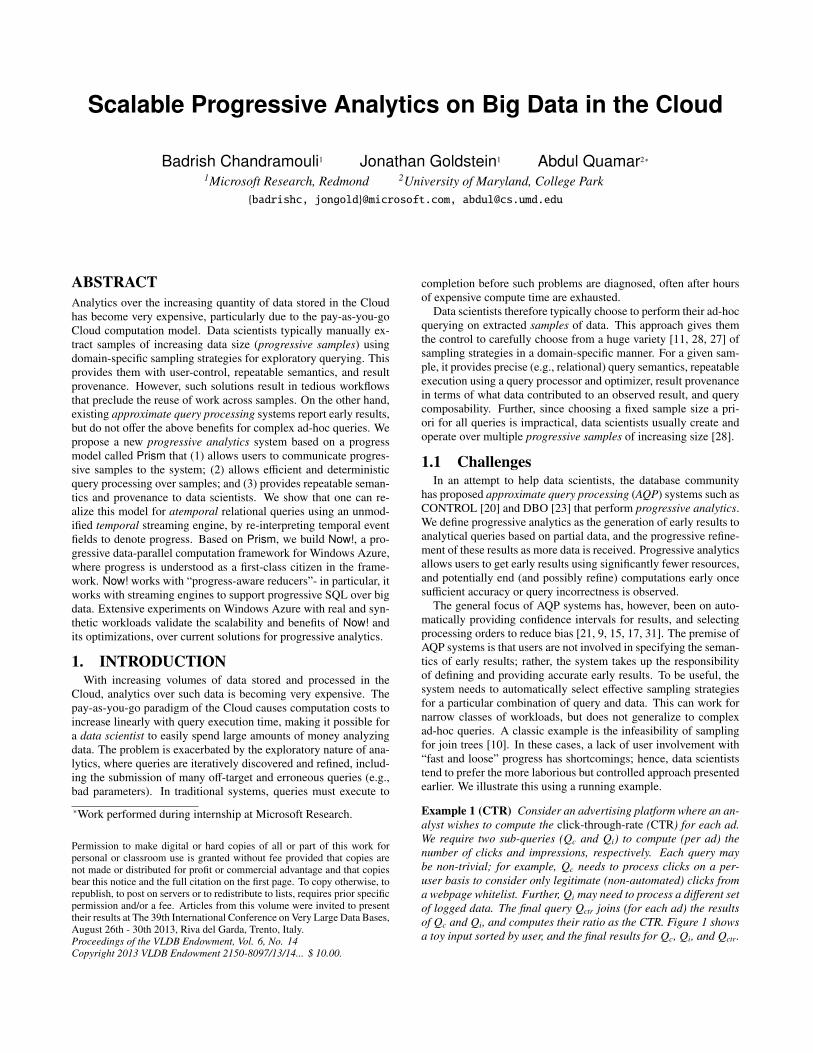
Example 1 (CTR) Consider an advertising platform where an an-alyst wishes to compute the click-through-rate (CTR) for each ad.We require two sub-queries (Qc and Qi) to compute (per ad) thenumber of clicks and impressions, respectively. Each query maybe non-trivial; for example, Qc needs to process clicks on a per-user basis to consider only legitimate (non-automated) clicks froma webpage whitelist. Further, Qi may need to process a different setof logged data. The final query Qctr joins (for each ad) the resultsof Qc and Qi, and computes their ratio as the CTR. Figure 1 showsa toy input sorted by user, and the final results for Qc, Qi, and Qctr.

User Ad . . .u0 a0 . . .u1 a0 . . .u2 a0 . . .

(a)

User Ad . . .u0 a0 . . .u0 a0 . . .u1 a0 . . .u2 a0 . . .u2 a0 . . .

(b)

Ad Clicksa0 3

Ad Imprsa0 5

(c)

Ad CTRa0 0.6

(d)Figure 1: (a) Click data; (b) Impression data; (c) Final result ofQc and Qi; (d) Final result of Qctr.

Next, Figure 3 (a) and (b) show progressive results for the samequeries Qc and Qi. Without user involvement in defining progres-sive samples, the exact sequence of progressive counts can be non-deterministic across runs, although the final counts are precise.Further, depending on the relative speed and sequence of resultsfor Qc and Qi, Qctr may compose arbitrary progressive results, re-sulting in significant variations in progressive CTR results. Fig-ures 3(c) and (d) show two possible results for Qctr. For example, aCTR of 2.0 would result from combining the first tuple from Qc andQi. Some results that are not even meaningful (e.g., CTR > 1.0)are possible. Although both results eventually get to the same finalCTR, there is no mechanism to ensure that the inputs being corre-lated to compute progressive CTRs are deterministic and compara-ble (e.g., computed using the same sample of users).

The above example illustrates several challenges:1) User-Control: Data scientists usually have domain expertise thatthey leverage to select from a range of sampling strategies [11, 28,27] based on their specific needs and context. In Example 1, wemay progressively sample both datasets identically in user-orderfor meaningful progress, avoiding the join sampling problem [10].Users may also need more flexibility; for instance, with a star-schema dataset, they may wish to fully process the small dimensiontable before sampling the fact table, for better progressive results.2) Semantics: Relational algebra provides precise semantics forSQL queries. Given a set of input tables, the correct output is de-fined by the input and query alone, and is independent of dynamicproperties such as the order of processing tuples. However, forcomplex queries, existing AQP systems use operational semantics,where early results are on a best-effort basis. Thus, it is unclearwhat a particular early result means to the user.3) Repeatability & Optimization: Two runs of a query in AQP mayprovide a different sequence of early results, although they haveto both converge to the same final answer. Thus, without limitingthe class of queries which are progressively executed, it is hard tounderstand what early answers mean, or even recognize anomalousearly answers. Even worse, changing the physical operators in theplan (e.g., changing operators within the ripple join family [16])can significantly change what early results are seen!4) Provenance: Users cannot easily establish the provenance ofearly results, e.g., link an early result (CTR=3.0) to particular con-tributing tuples, which is useful to debug and reason about results.5) Query Composition: The problem of using operational seman-tics is exacerbated when one starts to compose queries. Example 1shows that one may get widely varying results (e.g., spurious CTRvalues) that are hard to reason about.6) Scale-Out: Performing progressive analytics at scale exacer-bates the above challenges. The CTR query from Example 1 is

UserId UserId

AdId

Job partitioning

keys

Figure 2: CTR; MR jobs.

expressed as two map-reduce(MR) jobs that partition data byUserId, feeding a third job thatpartitions data by a different key(AdId); see Figure 2. In acomplex distributed multi-stageworkflow, accurate deterministicprogressive results can be very

Ad Clicksa0 2a0 3

(a)

Ad Imprsa0 1a0 4a0 5

(b)

Ad CTRa0 2.0a0 0.5a0 0.6

(c)

Ad CTRa0 3.0a0 0.75a0 0.6

(d)Figure 3: (a) Progressive Qc output; (b) Progressive Qi output;(c) & (d) Two possible progressive Qctr results.

useful. Map-reduce-online (MRO) [12] adds a limited form ofpipelining to MR, but MRO reports a heuristic progress metric (av-erage fraction of data processed across mappers) that does not elim-inate the problems discussed above (§ 6 covers related work).

To summarize, data scientists prefer user-controlled progressivesampling because it helps avoid the above issues, but the lack ofsystem support results in a tedious and error-prone workflow thatprecludes the reuse of work across progressive samples. We need asystem that (1) allows users to communicate progressive samples tothe system; (2) allows efficient and deterministic query processingover progressive samples, without the system itself trying to reasonabout specific sampling strategies or confidence estimation; and yet(3) continues to offer the desirable features outlined above.

1.2 Contributions

1) Prism: A New Progress Model & ImplementationWe propose (§ 2) a new progress model called Prism (Progressivesampling model). The key idea is for users to encode their cho-sen progressive sampling strategy into the data by augmenting tu-ples with explicit progress intervals (PIs). PIs denote logical pointswhere tuples enter and exit the computation, and explicitly assigntuples to progressive samples. PIs offer remarkable flexibility forencoding sampling strategies and ordering for early results, includ-ing arbitrarily overlapping sample sequences and special cases suchas the star-schema join mentioned earlier (§ 2.5 has more details).

PIs propagate through Prism operators. Combined with progres-sive operator semantics, PIs provide closed-world determinism: theexact sequence of early results is a deterministic function of aug-mented inputs and the logical query alone. They are independent ofphysical plans, which enables side-effect-free query optimization.Provenance is explicit; result tuples have PIs that denote the ex-act set of contributing inputs. Prism also allows meaningful querycomposition, as operators respect PIs. If desired, users can encodeconfidence interval computations as part of their queries.

The introduction of a new progress model into an existing re-lational engine appears challenging. However, interestingly, weshow (§ 2.4) that a progressive in-memory relational engine basedon Prism can be realized immediately using an unmodified tem-poral streaming engine, by carefully reusing its temporal fields todenote progress. Tuples from successive progressive samples getincrementally processed when possible, giving a significant perfor-mance benefit. Note here that the temporal engine is unaware thatit is processing atemporal relational queries; we simply re-interpretits temporal fields to denote progress points. While it may appearthat in-memory queries can be memory intensive since the finalanswer is computed over the entire dataset, Prism allows us to ex-ploit sort orders and foreign key dependencies in the input data andqueries to reduce memory usage significantly (§ 2.6).Prism generalizes AQP Our progress semantics are compatiblewith queries for which prior AQP techniques with statistical guar-antees apply, and thus don’t require user involvement. These tech-niques simply correspond to different PI assignment policies forinput data. For instance, variants of ripple join [16] are different PIassignments for a temporal symmetric-hash-join, with confidenceintervals computed as part of the query. Thus, Prism is orthogo-nal to and can leverage this rich area of prior work, while adding

PI User Ad[0,∞) u0 a0[1,∞) u1 a0[2,∞) u2 a0

(a)

PI User Ad[0,∞) u0 a0[0,∞) u0 a0[1,∞) u1 a0[2,∞) u2 a0[2,∞) u2 a0

(b)

PI Ad Clicks[0, 1) a0 1[1, 2) a0 2[2,∞) a0 3

PI Ad Imprs[0, 1) a0 2[1, 2) a0 3[2,∞) a0 5

(c)

PI Ad CTR[0, 1) a0 0.5[1, 2) a0 0.66[2,∞) a0 0.6

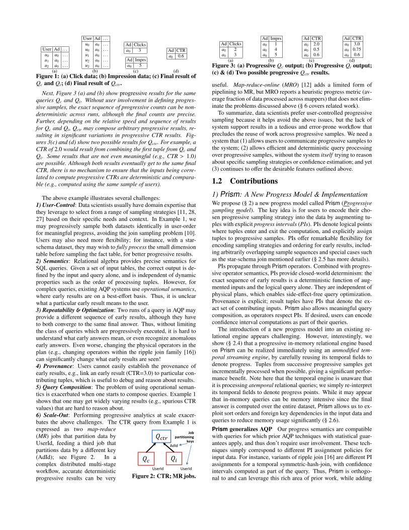
(d)Figure 4: (a,b) Input data with progress intervals; (c) Progres-sive results of Qc and Qi; (d) Progressive output of Qctr.

the benefit of repeatable and deterministic semantics. In summary,Prism gives progressive results the same form of determinism anduser control that relational algebra provides final results.

2) Applying Prism in a Scaled-Out Cloud SettingThe Prism model is particularly suitable for progressive analyticson big data in the Cloud, since queries in this setting are complex,and memory- and CPU-intensive. Traditional scalable distributedframeworks such as MR are not pipelined, making them unsuitablefor progressive analytics. MRO adds pipelining, but does not offerthe semantic underpinnings of progress necessary to achieve thedesirable features outlined earlier.

We address this problem by designing and building a new frame-work for progressive analytics called Now! (§ 3). Now! runs onWindows Azure; it understands and propagates progress (basedon the Prism model) as a first-class citizen inside the framework.Now! generalizes the popular data-parallel MR model and supportsprogress-aware reducers that understand explicit progress in thedata. In particular, Now! can work with a temporal engine (we useStreamInsight [3]) as a progress-aware reducer to enable scaled-outprogressive relational (SQL) query support in the Cloud. Now! is anovel contribution in its own right, with several important features:• Fully pipelined progressive computation and data movement across

multiple stages with different partitioning keys, in order to avoidthe high cost of sending intermediate results to Cloud storage.

• Elimination of sorting in the framework using progress-ordereddata movement, partitioned computation pushed inside progress-aware reducers, and support for the traditional reducer API.

• Progress-based merge of multiple map outputs at a reducer node.• Concurrent scheduling of multi-stage map and reduce jobs with

a new scheduling policy and flow control scheme.We also extend Now! (§ 4) with a high performance mode thateliminates disk writes, and discuss high availability (by leveragingprogress semantics in a new way) and straggler management.

We perform a detailed evaluation (§ 5) of Now! on WindowsAzure (with StreamInsight) over real and benchmark datasets up to100GB, with up to 75 large-sized Azure compute instances. Exper-iments show that we can scale effectively and produce meaningfulearly results, making Now! suitable in a pay-as-you-go environ-ment. Now! provides a substantial reduction in processing time,memory and CPU usage as compared to current schemes; perfor-mance is significantly enhanced by exploiting sort orders and usingour memory-only processing mode.

Paper Outline § 2 provides the details of our proposed modelfor progressive computation Prism. We present Now! in detail in§ 3; and discuss several extensions in § 4. The detailed evaluationof Now! is covered in § 5, and related work is discussed in § 6.

2. Prism SEMANTICS & CONSTRUCTIONAt a high level, our progress model (called Prism) defines a log-

ical linear progress domain that represents the progress of a query.Sampling strategies desired by data scientists are encoded into thedata before query processing, using augmented tuples with progress

0

Impression

Input Data

Progress Domain 1 2

1 2 3

2 3 5

0.5 0.66 0.6

Click

Input Data

Early results (on partial data) Final result (on full data)

Progress interval

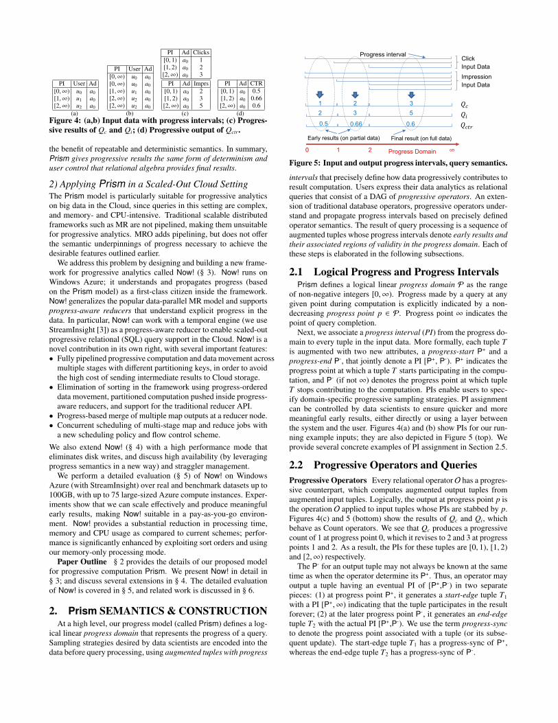
Figure 5: Input and output progress intervals, query semantics.

intervals that precisely define how data progressively contributes toresult computation. Users express their data analytics as relationalqueries that consist of a DAG of progressive operators. An exten-sion of traditional database operators, progressive operators under-stand and propagate progress intervals based on precisely definedoperator semantics. The result of query processing is a sequence ofaugmented tuples whose progress intervals denote early results andtheir associated regions of validity in the progress domain. Each ofthese steps is elaborated in the following subsections.

2.1 Logical Progress and Progress IntervalsPrism defines a logical linear progress domain P as the range

of non-negative integers [0,∞). Progress made by a query at anygiven point during computation is explicitly indicated by a non-decreasing progress point p ∈ P. Progress point ∞ indicates thepoint of query completion.

Next, we associate a progress interval (PI) from the progress do-main to every tuple in the input data. More formally, each tuple Tis augmented with two new attributes, a progress-start P+ and aprogress-end P-, that jointly denote a PI [P+, P-). P+ indicates theprogress point at which a tuple T starts participating in the compu-tation, and P- (if not ∞) denotes the progress point at which tupleT stops contributing to the computation. PIs enable users to spec-ify domain-specific progressive sampling strategies. PI assignmentcan be controlled by data scientists to ensure quicker and moremeaningful early results, either directly or using a layer betweenthe system and the user. Figures 4(a) and (b) show PIs for our run-ning example inputs; they are also depicted in Figure 5 (top). Weprovide several concrete examples of PI assignment in Section 2.5.

2.2 Progressive Operators and QueriesProgressive Operators Every relational operatorO has a progres-sive counterpart, which computes augmented output tuples fromaugmented input tuples. Logically, the output at progress point p isthe operation O applied to input tuples whose PIs are stabbed by p.Figures 4(c) and 5 (bottom) show the results of Qc and Qi, whichbehave as Count operators. We see that Qc produces a progressivecount of 1 at progress point 0, which it revises to 2 and 3 at progresspoints 1 and 2. As a result, the PIs for these tuples are [0, 1), [1, 2)and [2,∞) respectively.

The P- for an output tuple may not always be known at the sametime as when the operator determine its P+. Thus, an operator mayoutput a tuple having an eventual PI of [P+,P-) in two separatepieces: (1) at progress point P+, it generates a start-edge tuple T1

with a PI [P+,∞) indicating that the tuple participates in the resultforever; (2) at the later progress point P-, it generates an end-edgetuple T2 with the actual PI [P+,P-). We use the term progress-syncto denote the progress point associated with a tuple (or its subse-quent update). The start-edge tuple T1 has a progress-sync of P+,whereas the end-edge tuple T2 has a progress-sync of P-.

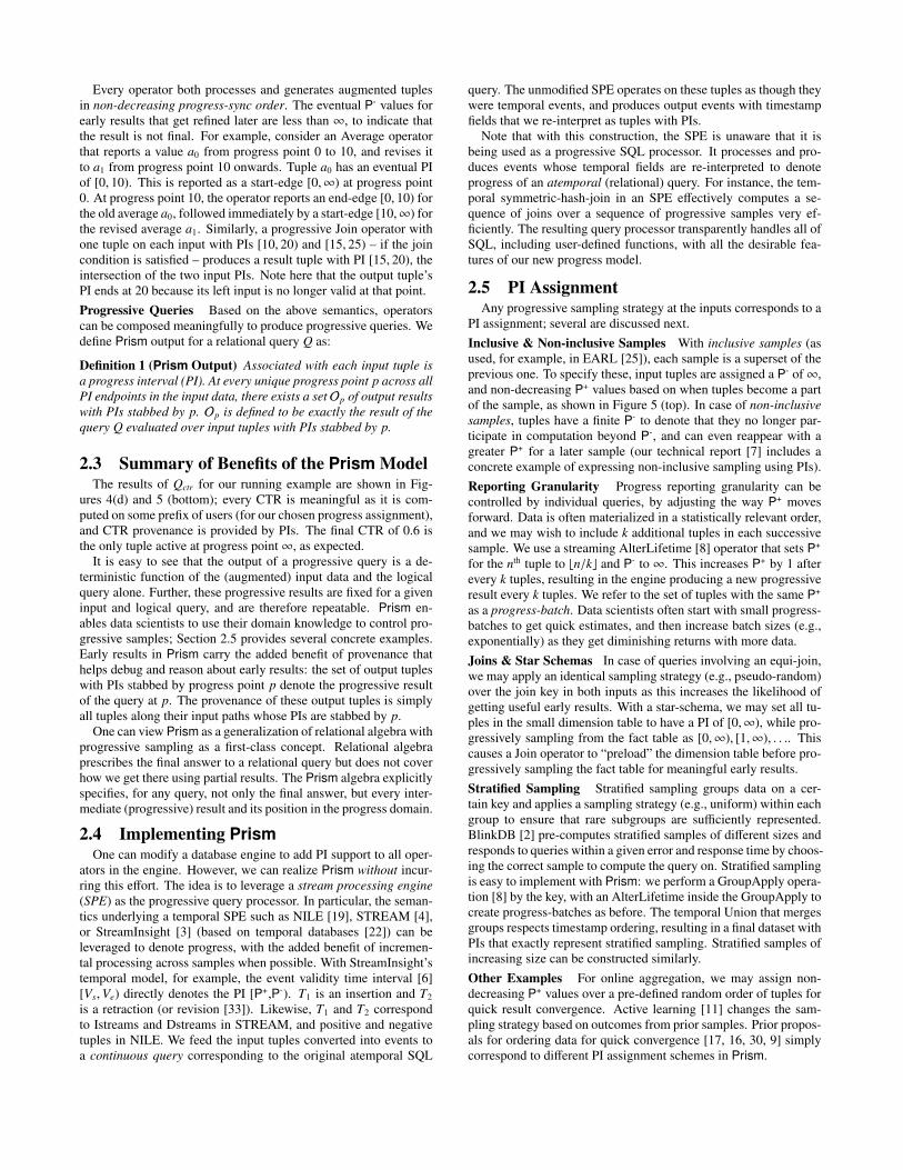
Every operator both processes and generates augmented tuplesin non-decreasing progress-sync order. The eventual P- values forearly results that get refined later are less than ∞, to indicate thatthe result is not final. For example, consider an Average operatorthat reports a value a0 from progress point 0 to 10, and revises itto a1 from progress point 10 onwards. Tuple a0 has an eventual PIof [0, 10). This is reported as a start-edge [0,∞) at progress point0. At progress point 10, the operator reports an end-edge [0, 10) forthe old average a0, followed immediately by a start-edge [10,∞) forthe revised average a1. Similarly, a progressive Join operator withone tuple on each input with PIs [10, 20) and [15, 25) – if the joincondition is satisfied – produces a result tuple with PI [15, 20), theintersection of the two input PIs. Note here that the output tuple’sPI ends at 20 because its left input is no longer valid at that point.Progressive Queries Based on the above semantics, operatorscan be composed meaningfully to produce progressive queries. Wedefine Prism output for a relational query Q as:

Definition 1 (Prism Output) Associated with each input tuple isa progress interval (PI). At every unique progress point p across allPI endpoints in the input data, there exists a set Op of output resultswith PIs stabbed by p. Op is defined to be exactly the result of thequery Q evaluated over input tuples with PIs stabbed by p.

2.3 Summary of Benefits of the Prism ModelThe results of Qctr for our running example are shown in Fig-

ures 4(d) and 5 (bottom); every CTR is meaningful as it is com-puted on some prefix of users (for our chosen progress assignment),and CTR provenance is provided by PIs. The final CTR of 0.6 isthe only tuple active at progress point∞, as expected.

It is easy to see that the output of a progressive query is a de-terministic function of the (augmented) input data and the logicalquery alone. Further, these progressive results are fixed for a giveninput and logical query, and are therefore repeatable. Prism en-ables data scientists to use their domain knowledge to control pro-gressive samples; Section 2.5 provides several concrete examples.Early results in Prism carry the added benefit of provenance thathelps debug and reason about early results: the set of output tupleswith PIs stabbed by progress point p denote the progressive resultof the query at p. The provenance of these output tuples is simplyall tuples along their input paths whose PIs are stabbed by p.

One can view Prism as a generalization of relational algebra withprogressive sampling as a first-class concept. Relational algebraprescribes the final answer to a relational query but does not coverhow we get there using partial results. The Prism algebra explicitlyspecifies, for any query, not only the final answer, but every inter-mediate (progressive) result and its position in the progress domain.

2.4 Implementing PrismOne can modify a database engine to add PI support to all oper-

ators in the engine. However, we can realize Prism without incur-ring this effort. The idea is to leverage a stream processing engine(SPE) as the progressive query processor. In particular, the seman-tics underlying a temporal SPE such as NILE [19], STREAM [4],or StreamInsight [3] (based on temporal databases [22]) can beleveraged to denote progress, with the added benefit of incremen-tal processing across samples when possible. With StreamInsight’stemporal model, for example, the event validity time interval [6][Vs,Ve) directly denotes the PI [P+,P-). T1 is an insertion and T2

is a retraction (or revision [33]). Likewise, T1 and T2 correspondto Istreams and Dstreams in STREAM, and positive and negativetuples in NILE. We feed the input tuples converted into events toa continuous query corresponding to the original atemporal SQL

query. The unmodified SPE operates on these tuples as though theywere temporal events, and produces output events with timestampfields that we re-interpret as tuples with PIs.

Note that with this construction, the SPE is unaware that it isbeing used as a progressive SQL processor. It processes and pro-duces events whose temporal fields are re-interpreted to denoteprogress of an atemporal (relational) query. For instance, the tem-poral symmetric-hash-join in an SPE effectively computes a se-quence of joins over a sequence of progressive samples very ef-ficiently. The resulting query processor transparently handles all ofSQL, including user-defined functions, with all the desirable fea-tures of our new progress model.

2.5 PI AssignmentAny progressive sampling strategy at the inputs corresponds to a

PI assignment; several are discussed next.Inclusive & Non-inclusive Samples With inclusive samples (asused, for example, in EARL [25]), each sample is a superset of theprevious one. To specify these, input tuples are assigned a P- of∞,and non-decreasing P+ values based on when tuples become a partof the sample, as shown in Figure 5 (top). In case of non-inclusivesamples, tuples have a finite P- to denote that they no longer par-ticipate in computation beyond P-, and can even reappear with agreater P+ for a later sample (our technical report [7] includes aconcrete example of expressing non-inclusive sampling using PIs).Reporting Granularity Progress reporting granularity can becontrolled by individual queries, by adjusting the way P+ movesforward. Data is often materialized in a statistically relevant order,and we may wish to include k additional tuples in each successivesample. We use a streaming AlterLifetime [8] operator that sets P+

for the nth tuple to bn/kc and P- to ∞. This increases P+ by 1 afterevery k tuples, resulting in the engine producing a new progressiveresult every k tuples. We refer to the set of tuples with the same P+

as a progress-batch. Data scientists often start with small progress-batches to get quick estimates, and then increase batch sizes (e.g.,exponentially) as they get diminishing returns with more data.Joins & Star Schemas In case of queries involving an equi-join,we may apply an identical sampling strategy (e.g., pseudo-random)over the join key in both inputs as this increases the likelihood ofgetting useful early results. With a star-schema, we may set all tu-ples in the small dimension table to have a PI of [0,∞), while pro-gressively sampling from the fact table as [0,∞), [1,∞), . . .. Thiscauses a Join operator to “preload” the dimension table before pro-gressively sampling the fact table for meaningful early results.Stratified Sampling Stratified sampling groups data on a cer-tain key and applies a sampling strategy (e.g., uniform) within eachgroup to ensure that rare subgroups are sufficiently represented.BlinkDB [2] pre-computes stratified samples of different sizes andresponds to queries within a given error and response time by choos-ing the correct sample to compute the query on. Stratified samplingis easy to implement with Prism: we perform a GroupApply opera-tion [8] by the key, with an AlterLifetime inside the GroupApply tocreate progress-batches as before. The temporal Union that mergesgroups respects timestamp ordering, resulting in a final dataset withPIs that exactly represent stratified sampling. Stratified samples ofincreasing size can be constructed similarly.Other Examples For online aggregation, we may assign non-decreasing P+ values over a pre-defined random order of tuples forquick result convergence. Active learning [11] changes the sam-pling strategy based on outcomes from prior samples. Prior propos-als for ordering data for quick convergence [17, 16, 30, 9] simplycorrespond to different PI assignment schemes in Prism.

Blob Blob Blob

Map Stage

Disk Disk Disk

Reduce StageMerge Merge Merge

Map Stage

Disk

Reduce StageMerge Merge Merge

Blob Blob Blob

Shuffle

ShuffleDisk Disk

Sort

Blob Blob Blob

Map Stage (Progress-aware batching)

Progressive Reducer (Gen API)Progress Aware Merge

Map Stage(Progress-aware batching)

Progressive Reducer (Gen API)Progress Aware Merge

Blob Blob Blob

Progressive data shuffle

No Sort

Blob Blob BlobIn Memory

data transfer

Progressive data shuffle

No Sort

(a) Vanilla MR (b) Now!

PI annotated

Input

Progressive Output

Figure 6: System architecture (MR vs. Now!).

2.6 Performance OptimizationsQuery processing using an in-memory streaming engine can be

expensive since the final answer is over the entire dataset. Prismenables crucial performance optimizations that can improve perfor-mance significantly in practical situations. Consider computationQc, which is partitionable by UserId. We can exploit the compile-time property that progress-sync ordering is the same as (or cor-related to) the partitioning key, to reduce memory usage and con-sequently throughput. The key intuition is that although every tu-ple with PI [P+,∞) logically has a P- of ∞, it does not contributeto any progress point beyond P+. Thus, we can temporarily setP- to P++1 before feeding the tuples to the SPE. This effectivelycauses the SPE to not have to retain information related to progresspoint P+ in memory once computation for P+ is done. The resulttuples have their P- set back to ∞ to retain the original query se-mantics (these query modifications are introduced using compile-time query rewrites). A similar optimization applies to equi-joins;see [7] for details. We will see in Section 5 that this optimizationcan result in orders-of-magnitude performance benefits.

We next discuss our new big data framework called Now!, thatimplements Prism for MR-style computation at scale in a distributedsetting (applying Prism to other models such as graphs is an inter-esting area of future work).

3. Now! ARCHITECTURE AND DESIGN

3.1 OverviewAt a high level, Now!’s architecture is based on the Map-Reduce

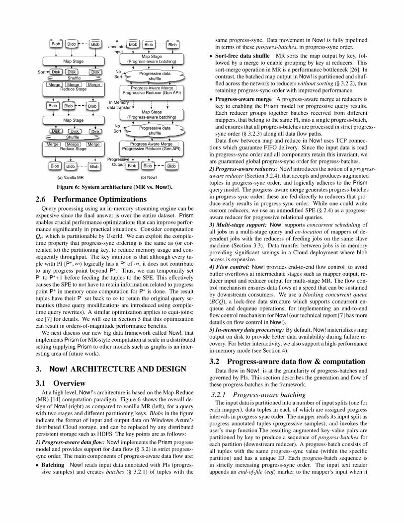
(MR) [14] computation paradigm. Figure 6 shows the overall de-sign of Now! (right) as compared to vanilla MR (left), for a querywith two stages and different partitioning keys. Blobs in the figureindicate the format of input and output data on Windows Azure’sdistributed Cloud storage, and can be replaced by any distributedpersistent storage such as HDFS. The key points are as follows:1) Progress-aware data flow: Now! implements the Prism progressmodel and provides support for data flow (§ 3.2) in strict progress-sync order. The main components of progress-aware data flow are:• Batching Now! reads input data annotated with PIs (progres-

sive samples) and creates batches (§ 3.2.1) of tuples with the

same progress-sync. Data movement in Now! is fully pipelinedin terms of these progress-batches, in progress-sync order.

• Sort-free data shuffle MR sorts the map output by key, fol-lowed by a merge to enable grouping by key at reducers. Thissort-merge operation in MR is a performance bottleneck [26]. Incontrast, the batched map output in Now! is partitioned and shuf-fled across the network to reducers without sorting (§ 3.2.2), thusretaining progress-sync order with improved performance.

• Progress-aware merge A progress-aware merge at reducers iskey to enabling the Prism model for progressive query results.Each reducer groups together batches received from differentmappers, that belong to the same PI, into a single progress-batch,and ensures that all progress-batches are processed in strict progress-sync order (§ 3.2.3) along all data flow paths.Data flow between map and reduce in Now! uses TCP connec-

tions which guarantee FIFO delivery. Since the input data is readin progress-sync order and all components retain this invariant, weare guaranteed global progress-sync order for progress-batches.2) Progress-aware reducers: Now! introduces the notion of a progress-aware reducer (Section 3.2.4), that accepts and produces augmentedtuples in progress-sync order, and logically adheres to the Prismquery model. The progress-aware merge generates progress-batchesin progress-sync order; these are fed directly to reducers that pro-duce early results in progress-sync order. While one could writecustom reducers, we use an unmodified SPE (§ 2.4) as a progress-aware reducer for progressive relational queries.3) Multi-stage support: Now! supports concurrent scheduling ofall jobs in a multi-stage query and co-location of mappers of de-pendent jobs with the reducers of feeding jobs on the same slavemachine (Section 3.3). Data transfer between jobs is in-memoryproviding significant savings in a Cloud deployment where blobaccess is expensive.4) Flow control: Now! provides end-to-end flow control to avoidbuffer overflows at intermediate stages such as mapper output, re-ducer input and reducer output for multi-stage MR. The flow con-trol mechanism ensures data flows at a speed that can be sustainedby downstream consumers. We use a blocking concurrent queue(BCQ), a lock-free data structure which supports concurrent en-queue and dequeue operations, for implementing an end-to-endflow control mechanism for Now! (our technical report [7] has moredetails on flow control in Now!).5) In-memory data processing: By default, Now! materializes mapoutput on disk to provide better data availability during failure re-covery. For better interactivity, we also support a high-performancein-memory mode (see Section 4).

3.2 Progress-aware data flow & computationData flow in Now! is at the granularity of progress-batches and

governed by PIs. This section describes the generation and flow ofthese progress-batches in the framework.

3.2.1 Progress-aware batchingThe input data is partitioned into a number of input splits (one for

each mapper), data tuples in each of which are assigned progressintervals in progress-sync order. The mapper reads its input split asprogress annotated tuples (progressive samples), and invokes theuser’s map function.The resulting augmented key-value pairs arepartitioned by key to produce a sequence of progress-batches foreach partition (downstream reducer). A progress-batch consists ofall tuples with the same progress-sync value (within the specificpartition) and has a unique ID. Each progress-batch sequence isin strictly increasing progress-sync order. The input text readerappends an end-of-file (eof) marker to the mapper’s input when it

PI User Ad[0,∞) u0 a0[0,∞) u0 a0[1,∞) u1 a0[1,∞) u1 a1[2,∞) u2 a1[2,∞) u2 a1[2,∞) u2 a1[2,∞) u2 a1

(a)

PI User Ad[0,∞) u0 a0[0,∞) u0 a0

PI User Ad[1,∞) u1 a0[1,∞) u1 a1

PI User Ad[2,∞) u2 a1[2,∞) u2 a1[2,∞) u2 a1[2,∞) u2 a1

(b)

PI User Ad[0,∞) u0 a0[0,∞) u0 a0[0,∞) u1 a0[0,∞) u1 a1

PI User Ad[1,∞) u2 a1[1,∞) u2 a1[1,∞) u2 a1[1,∞) u2 a1

(c)

Figure 7: (a) Input data annotated with PIs; (b) Progress-batches according to input data PI assignment; (c) Progress-batches with modified granularity using a batching function.

reaches the end of its input split. The mapper, on receipt of the eofmarker, appends it to all progress-batch sequences.Batching granularity. The batching granularity in the frameworkis determined by the PI assignment scheme (§ 2.5) of the inputdata. Now!, also provides a control knob to the user, in terms of aparameterized batching function, to vary the batching granularityof the map output as a factor of the PI annotation granularity of theactual input. This avoids re-annotating the input data with PIs if theuser decides to alter the granularity of the progressive output.

Example 2 (Batching) Figure 7(a) shows a PI annotated input splitwith three progressive samples. Figure 7(b) shows the correspond-ing batched map output, where each tuple in a batch has the sameprogress-sync value. Figure 7(c) shows how progress granularity isvaried using a batching function that modifies P+. Here, P+ = b P+

b c

is the batching function, with the batching parameter b set to 2.

3.2.2 Progressive data shuffleNow! shuffles data between the mappers and reducers in terms

of progress-batches without sorting. As an additional performanceenhancement, Now! supports a mode for in-memory transfer of databetween the mappers and reducers with flow control to avoid mem-ory overflow. We pipeline progress-batches from the mapper to thereducers using a fine-grained signaling mechanism, which allowsthe mappers to inform the job tracker (master) the availability of aprogress-batch. The job tracker then passes the progress-batch IDand location information to the appropriate reducers, triggering therespective map output downloads.

The download mechanism on the reducer side has been designedto support progress-sync ordered batch movement. Each reducermaintains a separate blocking concurrent queue (BCQ) for eachmapper associated with the job. As mentioned earlier, the BCQ is alock-free in-memory data structure which supports concurrent en-queue and dequeue operations and enables appropriate flow controlto avoid swamping of the reducer. The maximum size of the BCQis a tunable parameter which can be set according to the availablememory at the reducer . The reducer enqueues progress-batches,downloaded from each mapper, into the corresponding BCQ as-sociated with the mapper, in strict progress-sync order. Note thatour batched sequential mode of data transfer means that continuousconnections do not need to be maintained between mappers and re-ducers, which aids scalability.3.2.3 Progress-aware merge

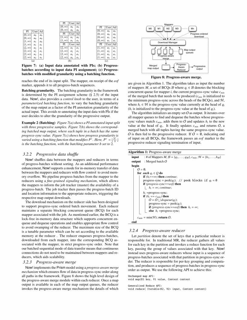
Now! implements the Prism model using a progress-aware mergemechanism which ensures flow of data in progress-sync order alongall paths in the framework. Figure 8 shows the high level design ofthe progress-aware merge module within each reducer. Once a mapoutput is available in each of the map output queues, the reducerinvokes the progress-aware merge mechanism the details of which

M0 M1 M2 M3 Mn

Download Manager

Map output queues

Progress ordered download

Mappers

Merged map output

Progress-Aware

ReducerProgressive

output

Progress-aware merge

Figure 8: Progress-aware merge.

are given in Algorithm 1. The algorithm takes as input the numberof mappers M, a set of BCQs B where qi ∈ B denotes the blockingconcurrent queue for mapper i, the current progress-sync value cmin

of the merged batch that needs to be produced (cmin is initialized tothe minimum progress-sync across the heads of the BCQs), andH ,where hi ∈ H is the progress-sync value currently at the head of qi

(hi is initialized to the progress-sync value at the head of qi).The algorithm initializes an empty setO as output. It iterates over

all mapper queues to find and dequeue the batches whose progress-sync values match cmin, adds them to O and updates hi to the newvalue at the head of qi. It finally updates cmin and returns O, amerged batch with all tuples having the same progress-sync value.O is then fed to the progressive reducer. If O = ∅, indicating endof input on all BCQs, the framework passes an eof marker to theprogressive reducer signaling termination of input.

Algorithm 1: Progress-aware mergeinput : # of Mappers M,B = {q1, . . . , qM}, cmin,H = {h1, . . . , hM}

output : Merged batch ObeginO = ∅;for each qi ∈ Q do

if (hi==∞) then continue;progress-sync = peek(qi); // peek blocks if qi = ∅if (progress-sync==eof) then

hi = ∞; continue;

hi =progress-sync;if (hi == cmin) thenO = O

⋃dequeue(qi);

progress-sync = peek(qi);if (progress-sync==eof) then hi = ∞;else hi =progress-sync;

cmin = min(H); return O;end

3.2.4 Progress-aware reducerLet partition denote the set of keys that a particular reducer is

responsible for. In traditional MR, the reducer gathers all valuesfor each key in the partition and invokes a reduce function for eachkey, passing the group of values associated with that key. Now!instead uses progress-aware reducers whose input is a sequence ofprogress-batches associated with that partition in progress-sync or-der. The reducer is responsible for per-key grouping and computa-tion, and produces a sequence of progress-batches in progress-syncorder as output. We use the following API to achieve this:

Unchanged map API:void map(K1 key, V1 value, Context context

Generalized Reduce API:void reduce( Iterable<K2, V2> input, Context context)

Algorithm 2: Schedulinginput : R f ,Ro,Mi,Md , dependency table

beginfor each r ∈ R f do

Dispatch r;if Dispatch successful then Make a note of tracker ID;

for each r ∈ Ro do Dispatch r;for each m ∈ Md do

Dispatch m, co-locating it with its feeder reducer;

for each m ∈ Mi doDispatch m closest to input data location;

end

Here, V1 and V2 include PIs. Now! also supports the traditionalreducer API to support older workflows, using a layer that groupsactive tuples by key for each progress point, invokes the traditionalreduce function for each key, and uses the reduce output to generatetuples with PIs corresponding to that progress point.Progressive SQL While users can write custom progress-awarereducers, we advocate using an unmodified temporal streaming en-gine (such as StreamInsight) as a reducer to handle progressive re-lational queries (§ 2.4). Streaming engines process data in times-tamp order, which matches with our progress-sync ordered datamovement. Temporal notions in events can be reinterpreted asprogress points in the query. Further, streaming engines naturallyhandle efficient grouped subplans using hash-based key partition-ing, which is necessary to process tuples in progress-sync order.

3.3 Support for Multi-stageWe find that most analytics queries need to be expressed as multi-

stage MR jobs. Now! supports a fully pipelined progressive jobexecution across different stages using concurrent job schedulingand co-location of processes that need to exchange data across jobs.Concurrent Job Scheduling The scheduler in Now! has beendesigned to receive all the jobs in a multi-stage query as a job graph,from the application controller. Each job is converted into a set ofmap and reduce tasks. The scheduler extracts the type informationfrom the job to construct a dependency table that tracks, for eachtask within each job, where it reads from and writes to (a blobsor some other job). The scheduler uses this dependency table topartition map tasks into a set of independent map tasks Mi whichread their input from a blob/HDFS, and a set of dependent maptasks Md whose input is the output of some previous stage reducer.Similarly, reduce tasks are partitioned into a set of feeder tasks R f

that provide output to mappers of subsequent jobs, and a set ofoutput reduce tasks Ro that write their output to a blob/HDFS.

Algorithm 2 shows the details of how the map and reduce taskscorresponding to different jobs are scheduled1. First, all the re-duce tasks in R f are scheduled on slave machines that have at leastone map slot available to schedule a corresponding dependent maptask in Md which would consume the feeder reduce task’s output.The scheduler maintains a state of the task tracker IDs of the slavemachines on which these feeder reduce tasks have been scheduled.Second, all the reducers in Ro are scheduled depending on the avail-ability of reduce slots on various slave machines in a round robinmanner. Third, all the map tasks in Md are dispatched, co-locating

1If the scheduler is given additional information such as the stream-ing query plan executing inside reducers, we may be able to lever-age database cost estimation techniques to improve the schedulingalgorithm. This is a well studied topic in prior database research,and the ideas translate well to our setting.

J3

J2

J1

Data input

Final output

Data flow

Initial Job

Intermediate Job

Final Job

M1 M2 M3

R1 R2

M1 M2

R1 R2

M1 M2

R1 R2

F1 F2 F3 Input Files

O1 O2 Output Files

Blocking Concurrent

Queue

Blocking Concurrent

Queue

(a) (b)Task placement

J2

J1

J3

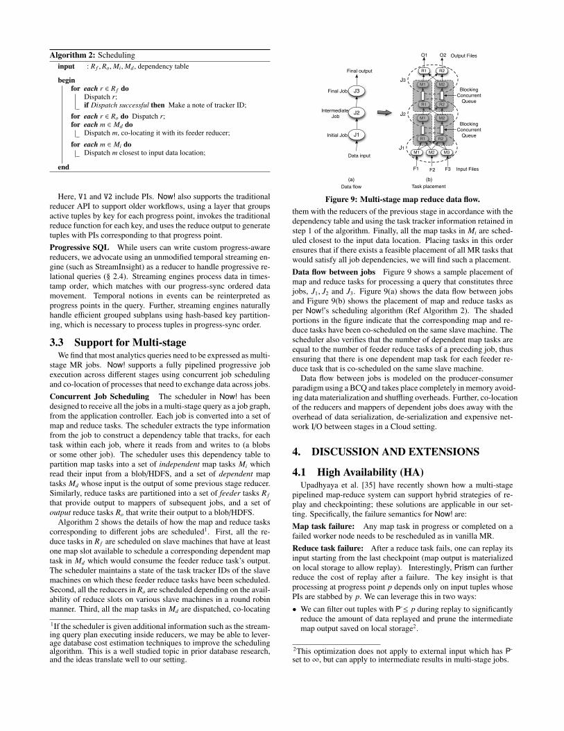
Figure 9: Multi-stage map reduce data flow.them with the reducers of the previous stage in accordance with thedependency table and using the task tracker information retained instep 1 of the algorithm. Finally, all the map tasks in Mi are sched-uled closest to the input data location. Placing tasks in this orderensures that if there exists a feasible placement of all MR tasks thatwould satisfy all job dependencies, we will find such a placement.Data flow between jobs Figure 9 shows a sample placement ofmap and reduce tasks for processing a query that constitutes threejobs, J1, J2 and J3. Figure 9(a) shows the data flow between jobsand Figure 9(b) shows the placement of map and reduce tasks asper Now!’s scheduling algorithm (Ref Algorithm 2). The shadedportions in the figure indicate that the corresponding map and re-duce tasks have been co-scheduled on the same slave machine. Thescheduler also verifies that the number of dependent map tasks areequal to the number of feeder reduce tasks of a preceding job, thusensuring that there is one dependent map task for each feeder re-duce task that is co-scheduled on the same slave machine.

Data flow between jobs is modeled on the producer-consumerparadigm using a BCQ and takes place completely in memory avoid-ing data materialization and shuffling overheads. Further, co-locationof the reducers and mappers of dependent jobs does away with theoverhead of data serialization, de-serialization and expensive net-work I/O between stages in a Cloud setting.

4. DISCUSSION AND EXTENSIONS

4.1 High Availability (HA)Upadhyaya et al. [35] have recently shown how a multi-stage

pipelined map-reduce system can support hybrid strategies of re-play and checkpointing; these solutions are applicable in our set-ting. Specifically, the failure semantics for Now! are:Map task failure: Any map task in progress or completed on afailed worker node needs to be rescheduled as in vanilla MR.Reduce task failure: After a reduce task fails, one can replay itsinput starting from the last checkpoint (map output is materializedon local storage to allow replay). Interestingly, Prism can furtherreduce the cost of replay after a failure. The key insight is thatprocessing at progress point p depends only on input tuples whosePIs are stabbed by p. We can leverage this in two ways:

• We can filter out tuples with P-≤ p during replay to significantlyreduce the amount of data replayed and prune the intermediatemap output saved on local storage2.

2This optimization does not apply to external input which has P-

set to∞, but can apply to intermediate results in multi-stage jobs.

• During replay, we can set P+= max(p, P+) for replayed tuplesso that the reducer does not need to re-generate early results forprogress points earlier than p.Prior research [32] has reported that input sizes on production

clusters are usually less than 100GB. Further, progressive queriesare usually expected to end early. Therefore, Now! supports an ef-ficient no-HA mode, where intermediate map output is not materi-alized on local storage and no checkpointing is done. This requiresa failure to cascade back to the source data (we simply restart thejob). Restarting the job on failure is a cheap and practical solu-tion for such systems as compared to traditional long-running jobs.That said, we acknowledge that high availability with low recoverytime (e.g., by restarting only the failed parts of the DAG) is impor-tant in some cases. Prior work [35, 38] has studied this problem;these ideas apply in our setting. We leave the implementation andevaluation of such fine-grained HA in Now! as future work.

4.2 Straggler and Skew ManagementStragglers A consequence of progress-sync merge is that if aprevious task makes slow progress, we need to slow down overallprogress to ensure global progress-sync order. While progress-syncorder is necessary to derive the benefits of Prism, there are fixesthat avoid sacrificing semantics and determinism:• Consider n nodes with 1 straggler. If the processing skew is a

result of imbalanced load, we can dynamically move partitionsfrom the straggler to a new node (we need to also move reducerstate). We may instead fail the straggler altogether and re-start itscomputation by partitioning its load equally across the remainingn − 1 nodes. The catch-up work gets done n − 1 times faster,resulting in a quicker restoration of balance 3.

• We could add support for compensating reducers, which cancontinue to process new progress points, but maintain enoughinformation to revise or compensate their state once late data isreceived. Several engines have discussed support for compensa-tions [6, 33], and fit well in this setting.

As we have not found stragglers to be a problem in our experimentson Windows Azure VMs, the current version of Now! does not ad-dress this issue. A deeper investigation is left as future work.Data Skew Data skew can result from several reasons:• Some sampling strategies encoded using PIs may miss out on

outliers or rare sub-populations within a population. This canbe resolved using stratified sampling which can be easily imple-mented in Prism as discussed in Section 2.5.

• Skew in the data may result in some progress-batches being largerthan others at the reducers. However, this is no different fromskew in traditional map-reduce systems, and solutions such as [24]are applicable here.

Since skew is closely related to the straggler problem, techniquesmentioned earlier for stragglers may also help mitigate skew.

5. EVALUATION5.1 Implementation Details

Now! is written in C# and deployed over Windows Azure. Now!uses the same master-slave architecture as Hadoop [36] with Job-Tracker and TaskTracker nodes. TaskTracker nodes are allocated afixed number of map and reduce slots. Heartbeats are used to en-sure that slave machines are available. We modified and extended

3If failures occur halfway through a job on average, jobs run for2.5/(n − 1) times as long due to a straggler with this scheme.

this baseline to incorporate our new design features (see Section 3)such as pipelining, progress-based batching, progress-sync merge,multi-stage job support, concurrent job scheduling, etc. Now! de-ployed on the Windows Azure Cloud platform, uses Azure blobsas persistent storage and Azure VM roles as JobTracker and Task-Tracker nodes. Multi-stage job graphs are generated by users andprovided to Now!’s JobTracker as input; each job consists of inputfiles, a partitioning key (or mapper), and a progressive reducer. Al-though Now! has been developed in C# and evaluated on WindowsAzure, its design features are not tied to any specific platform. Forexample, Now! could be implemented over Hadoop using HDFSand deployed on the Amazon EC2 cloud.

Now! makes it easy to employ StreamInsight as a reducer for pro-gressive SQL, by providing an additional API that allow users todirectly submit a graph of 〈key, query〉 pairs, where query is a SQLquery specified using LINQ [34]. Each node in this graph is auto-matically converted into a job. The job uses a special progressivereducer that uses StreamInsight to process tuples. The Now! APIcan be used to build front-ends that automatically convert largerHive, SQL, or LINQ queries into job graphs. Although the systemhas been designed for the Cloud and uses Cloud storage, it alsosupports deployment on a cluster of machines (or private Cloud).Now! includes diagnostics for monitoring CPU, memory, and I/Ousage statistics. These statistics are collected by an instance of alog manager running on each machine which outputs these in theform of logs which are stored as blobs in a separate container.

5.2 Experimental SetupSystem Configuration The input and final output of a job graphare stored in Azure blobs. Each Azure VM role (instance) is a large-sized machine with 4 1.6GHz cores, 7GB RAM, 850GB of localstorage, and 400Mbps allocated I/O bandwidth. Each instance wasconfigured to support 5 map slots and 2 reduce slots. We experi-ment with up to 75 instances in our tests4.Datasets We use the following datasets in our evaluation, withdataset sizes based upon the aggregate amount of memory neededto run our queries over them:

• Search data. This is a real 100GB search dataset from Bing, thatconsists of userids and their search terms. The input splits werecreated by sharding the data into a number of files/partitions, andannotating with fine-grained PI values.

• TPC-H data. We used the dbgen tool to generate a 100GB TPC-H benchmark dataset, for experiments using TPC-H queries.

• Click data. This is a real 12GB dataset from the Microsoft Ad-Center advertising platform, that comprises of clicks and impres-sions on various ads over a 3 month period.

Queries We use the following progressive queries:

• Top-k correlated search. The query reports the top-k words thatare most correlated with an input search term, according to agoodness score, in the search dataset. The query consists of twoNow! jobs, one feeding the other. The first stage job uses thedata set as input and partitions by userid. Each reducer com-putes a histogram that reports, for each word, the number ofsearches with and without the input term, and the total number ofsearches. The second stage job groups by word, and aggregatesthe histograms from the first stage, computes a per-word good-ness, and performs top-k to report the k most correlated words tothe input term. We use “music” as the default term.

4Our Windows Azure subscription allowed no more than 300cores; this limited us to 75 4-core VM instances.

0 20 40 60 80 100

0

50

100

150

200

Progress %

Tim

e ta

ken

(m

ins)

Effect of progressive computation

SMR: 8GB

Now!: 8GB

SMR: 6GB

Now!: 6GB

(a)

80 600 1200 6000

0

20

40

60

80

100

Batch Size (MB)

Qu

ery

pro

cess

ing

tim

e (m

ins)

Effect of batch size

MR

SMR

Now!

Time to first batch (Now!)

(b)

30GB 15GB

0

20

40

60

80

100

% T

ime

take

n

Performance AnalysisWrite to Blob

2nd Stage Reduce

2nd Stage Map D/n loads

2nd Stage Map

1st Stage Reduce

1st Stage Map D/n loads

1st Stage Map

Input enumeration

(c)

0

10

20

30

40

50

3 5 6 8 9 13 15 30

1

10

100

1000

10000

Scal

e-U

p f

acto

r

Data size (GB)

Qu

ery

pro

cess

ing

tim

e (m

ins)

Lo

g sc

ale

Scalability with increase in data size

SMR

Now!

Scale-up

(d)

20(1X)

30(1.5X)

45(2.25X)

60(3X)

74(3.7X)

123456

# Machines

Thro

ugh

pu

t sc

ale

-up

fa

cto

r

Throughput Scalability

Scale up: Now!

(e)

0

25

50

75

100

Map

ou

tpu

t sh

uff

le t

ime

(in

sec

s)

Effect of map output materialization

Map o/p in-memory

Map o/p on disk

(f)

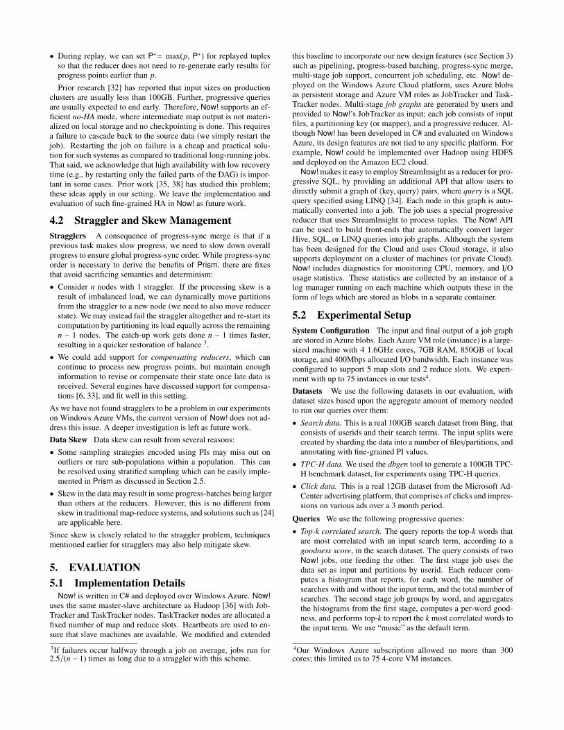
Figure 10: Performance analysis.(a) Time taken to process a query in progress-sync order; (b) Effect of batching granularity; (c)Analysis of time taken by different elements for a two-stage Map-Reduce query. Scalability: (d) Effect of data size on query processingtime; (e) Throughput scalability with increase in #machines; (f) Overheads of disk I/O (Map output materialization).

• TPC-H Q3. We use a generalization of TPC-H query 3:SELECT L_ORDERKEY, SUM(L_EXTENDEDPRICE*(1-L_DISCOUNT)) ASREVENUE, O_ORDERDATE, O_SHIPPRIORITY FROM ORDERS, LINEITEMWHERE L_ORDERKEY = O_ORDERKEYGROUP BY L_ORDERKEY, O_ORDERDATE, O_SHIPPRIORITY

• CTR. The CTR (click-through-rate) query computes the MR jobgraph shown in Figure 2 (our running example). It consists ofthree queries (Qc, Qi, and Qctr) where Qc is a click query whichcomputes the number of clicks from the click dataset, Qi is animpressions query which computes the number of ad impressionsfrom the impression data set and Qctr computes the CTR.

Baselines We evaluate Now! against several baseline systems:

• Map-Reduce (MR). For standard map-reduce, we use Daytona [13],a C# implementation of vanilla hadoop for Windows Azure. Thisbaseline provides an estimate of time taken to process a parti-tioned query without progressive results.

• Stateful MR (SMR). Stateful MR is an extension of MR for it-erative queries [5], that maintains reducer state across MR jobs.We use it for progressive results by chunking the input into batches,and submitting each chunk (in progress-sync order) as a separateMR job. Subsequent chunks use reducers that retain the priorjob’s state. For each chunk, we run each MR stage as a vanillaMR job. With multi-stage jobs, we process one chunk throughall stages before submitting the next chunk to the first stage.

• MRO [12]. MRO pipelines data between the mappers and re-ducers, but is unaware of progress semantics and does not useprogress-sync merge at the reducers. This can lead to differentnodes progressing at different speeds. We approximate MRO inNow! by replacing the progress-aware merge with a union5.

Job configuration and parameter settings. The configurationfor a two-stage job (with one job feeding another) is depicted asM1−R1−M2−R2 where M and R represent the number of mappers

5This baseline benefits from our other optimizations such as con-current job scheduling, no sorting, and pipelining across stages.

and reducers and their subscripts (1, 2) represent the stage to whichthey belong (note that R1 = M2). A single stage job is depicted asM1 −R1. In our experiments, the number of mappers is equal to thenumber of input splits (stored as blobs). The number of reducers ischosen based on the memory capacity of each worker node (7GBRAM) and the number of mappers feeding the reducers.

5.3 Experiments and Results5.3.1 Effect of Progressive Computation

We evaluate Now!’s performance vs. SMR in terms of timetaken to produce progressive results. The first experiment (see Fig-ure 10(a)) plots the time taken to run the top-k correlated searchquery which provides the top 100 words that were searched with“weather”, in terms of progress-batches plotted in progress-sync or-der. The input data set was batched by the mapper into 75 progress-batches by Now!. For the SMR baseline, the data was ordered andsplit into 75 chunks (one per PI). Each chunk representing one PI,was processed as a separate MR job and the time taken taken forthe same was recorded. Each point on the plot represents an aver-age of five runs. We used datasets of two sizes (6 and 8GB). Theexperimental results show that Now! performs much better (6X im-provement) than SMR, which processes each progress batch as aseparate job and resorts to expensive intermediate output material-ization, hurting performance, particularly in a Cloud setting. Also,the time taken for the first 50% of the progress batches is under20mins as opposed to 105mins for SMR, for the 8GB dataset, high-lighting the benefit of platform support for progressive early results.

5.3.2 Effect of BatchingWe evaluate the performance of Now! for different progress-

batch sizes and compare the same with SMR and MR. The MRbaseline processes the entire input as a single batch. The granu-larity of batch size controls the number of progress batches. Thedataset size used in this experiment is 6GB and the configuration is94-26-26-4. The experiment shows the results for 3 different batchsizes: 80MB (75 batches), 600MB (10 batches) and 1200MB (5

0

50

100

150

200

250

300

0 20 40 60 80 100

0

500

1000

1500

2000

% C

PU

Uti

l

Progress (% Time elasped)

Mem

ory

Uti

l (M

B)

Resource Util: Now! (94-26-26-4)Memory Util Mean (Memory Util)CPU Util Mean (CPU Util)

Time taken : 19 mins 4secs

(a)

0

50

100

150

200

250

300

0 20 40 60 80 100

0

500

1000

1500

% C

PU

Utiliz

atio

n

Progress (% Elapsed time)

Mem

ory

Uti

l (M

B)

Resource Utilization: SMR (94-26-26-4)Memory Util Mean (Memory Util)CPU Util Mean (CPU Util)Normalized CPU Util

Time taken : 86 mins 20 secs

(b)

0

50

100

150

200

250

300

0 20 40 60 80 100

0

1000

2000

3000

4000

5000

% C

PU

Uti

lizat

ion

Progress (% Elapsed time)

Mem

ory

Uti

l (M

B)

Resource Util: Now! (No Mem opt)Memory Util Mean (Mem Util)

CPU Util Mean (CPU Util)

Normalized CPU Util Time taken: 53 mins

(c)

0

50

100

150

200

250

300

0 20 40 60 80 100

0

100

200

300

400

% C

PU

Uti

lizat

ion

Progress (% Elapsed time)

Mem

ory

Uti

l (M

B)

Resource Util: Now! (Mem opt)Memory Util Mean (Mem Util)

% CPU Util Mean (CPU Util)

Time taken: 4 mins 26 secs

(d)

0

200

400

600

800

1000

1200

10GB (10 machines) 60GB (60 machines)

0

1

2

3

4

% C

PU

Uti

l

Mem

ory

Uti

l (G

B)

Effect of sort order: Resource UtilMemory Util* Normalized CPU Util

Memory Util Normalized CPU Util *

* With memory optimization

(e)

1

10

100

1000

10GB (10 m/cs) 60GB (60 m/cs) 100GB (74 m/cs)

Tim

e ta

ken

(m

ins)

Lo

g sc

ale

Effect of Sort Order: X-put scalabilityTime taken * Time taken

* With memory optimization

4.43mins

53mins

14.83mins

189mins

18.15mins

Out ofmemory

Scale-up:12X Scale-up:12.8X

(f)

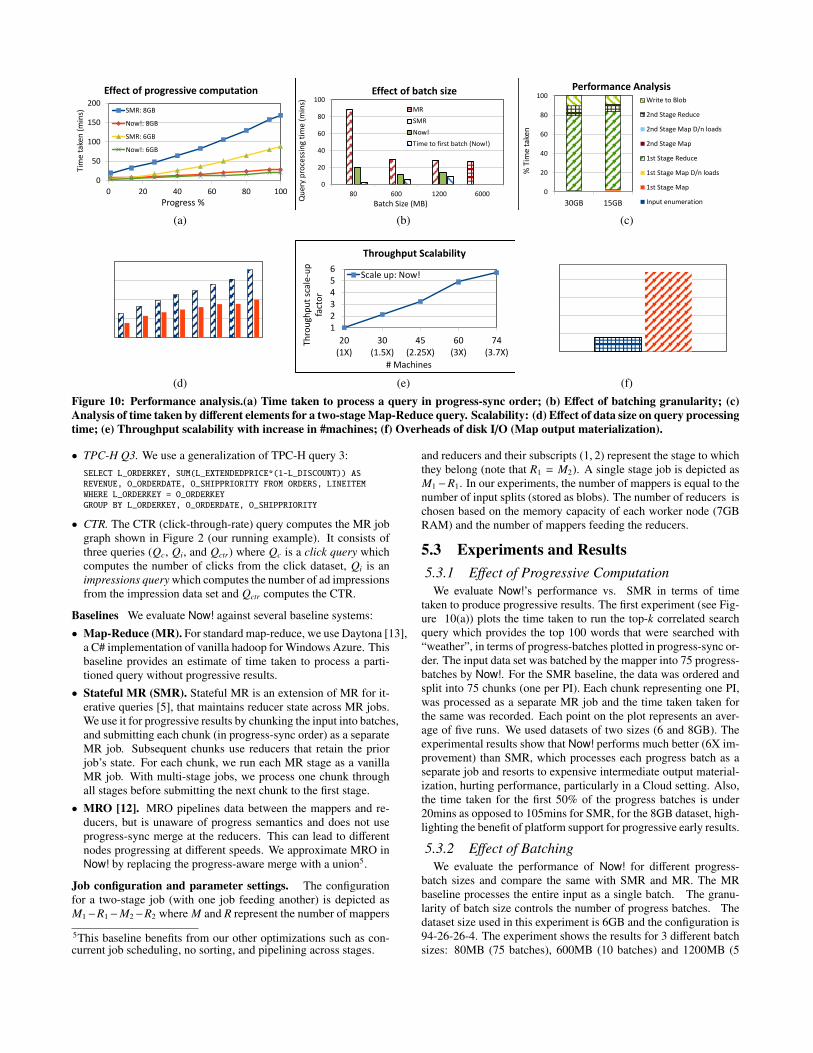
Figure 11: Resource Utilization. (a) CPU and memory utilization Now!; (b) CPU and memory utilization SMR;(c) CPU and memoryutilization without memory optimization; (d) CPU and memory utilization with memory optimization. (e) Effect of sort order onmemory and % CPU utilization for different data sizes; (f) Memory optimization effects on query processing time.

batches), and compares them against vanilla MR which processesthe entire input of 6GB at once.

Figure 10(b) shows the change in total query processing timewith change in batch size. As the batch-size decreases from 1200MBto 80MB, the number of batches processed by the system increasesfrom 5 to 75. The query processing time of SMR increases dras-tically with the increase in the number of batches, which can beattributed to the fact that it processes each batch as a separate MRjob and resorts to intermediate data materialization. The MR base-line which processes the entire input as a single batch does betterthan SMR , but does not provide early results.

On the other hand, the query processing time for Now! does notvary much with increase in number of batches as it is pipelined,does not start a new MR job for each batch, and does not material-ize intermediate results between jobs. We do see a slight increase inquery processing time when the number of batches increases from10 to 75, which can be attributed to a moderate increase in batchingoverheads. However, the smallest batch-size provides the earliestprogressive results and at the finest granularity. The figure showsthe time to generate the first progress batch i.e., the time when theuser starts getting progressive results. The time to first batch in-creases with increase in batch size (or progressive sample size), butis significantly lower than the total query processing time.

5.3.3 Performance BreakdownWe analyzed the performance of Now! using our diagnostic mon-

itoring module which logs CPU, memory, and I/O usage. Fig-ure 10(c) analyses the performance of the two-stage top-k corre-lated search query with k = 100, and plots the % time taken by dif-ferent components in Now!. Each data point in the figure is an av-erage over 10 runs, for two different datasets (15GB and 30GB) on30 machines. The results indicate that the maximum time is spentin the first stage reducer followed by the second stage reduce andwriting the final output to the blobs. The framework does not haveany major bottlenecks in terms of pipelining of progress-batches.The time taken by the two reduce stages would vary depending on

the choice of progressive reducer and the type of query. Our currentresults use StreamInsight as the progressive reducer.

5.3.4 ScalabilityFigure 10(d) evaluates the effect of increase in data size on query

processing time in Now! as compared to SMR. We used the top-k correlated search query for the experiment and varied the datasize from 2.8GB to 30GB. The results show that Now! provides ascale-up of up to 38X over SMR in terms of the ratio of their queryprocessing times. This can be attributed to pipelining, no sortingin the framework and no intermediate data materialization betweenjobs. Figure 10(e) shows the scale-up provided by Now! in terms ofthroughput (#rows processed per second) with the increase in #ma-chines. For the top-k correlated search query (top 100 words corre-lated to “music”), we achieved a 6X scale-up with 74 machines ascompared to the throughput on 20 machines, for 15GB data.

5.3.5 Data Materialization OverheadsWriting map outputs on the local disk, has a significant perfor-

mance penalty, while on the other hand, intermediate data material-ization provides higher availability in presence of failures . Figure10(f) shows the overhead of disk I/O in materializing map outputon disk and subsequent disk access to shuffle the data to the reduc-ers within a job. Our results show an overhead of approx 90 secsfor a dataset of 8GB for the 94-26-26-4 configuration.

Now! is tunable to work in both modes (with and without diskI/O) and can be chosen by the user depending on the applicationneeds and the execution environment. It is also pertinent to notehere that there is no data materialization on persistent storage (HDFSor Cloud) between different Map-Reduce stages in Now! whichprovides a similar performance advantage for multi-stage jobs overMR/SMR as seen in section 5.3.1.

5.3.6 Resource UtilizationWe evaluated Now! for its resource utilization in terms of mem-

ory and CPU. Figures 11(a,b) compare the memory and CPU uti-lization of Now! and SMR for the 94-26-26-4 configuration for a

dataset size of 8GB. The figures show the average real time memoryand CPU utilization over 30 slave machines each running 4 map-pers and 1 reducer plotted against time. The results indicate thatthere is no significant difference in the average memory utiliza-tion for both platforms, and the average CPU utilization of Now!is actually higher than that of SMR. However, we also show thenormalized %CPU utilization for SMR which is the product of theaverage CPU utilization and the normalization factor (ratio of timetaken by SMR to the time taken by Now!.) The normalized %CPUutilization is much higher as SMR takes approx 4.5X more time tocomplete as compared to Now!. Thus, Now! is ideal for progressivecomputation on the Cloud, where resources are charged by time.

5.3.7 Memory Optimization using Sort OrdersThe next experiment investigates the benefit of our memory op-

timization (cf. Section 2.6) in case the progress-sync order is cor-related with the partitioning key. Our TPC-H dataset uses progressin terms of the L ORDERKEY attribute, and TPC-H Q3 also parti-tions by the same key. An optimized run can detect this at compile-time and set P-=P++1, allowing the query to “forget” previous tu-ples when we move to the next progress-batch. An unoptimizedrun would retain all tuples in memory in order to compute futurejoin and aggregation results. We experiment with 10GB, 60GB and100GB TPC-H datasets. Figures 11(c) and 11(d) show the varia-tion of memory and CPU utilization with progress with and with-out memory optimization for the 10GB dataset. Figure 11(e) showsthat the memory footprint of the optimized approach is much lowerthan the unoptimized approach, as expected. Further, it indicatesthat the lower memory utilization directly impacts CPU utilizationsince the query needs to maintain and lookup much smaller joinsynopses. Figure 11(f) shows that memory optimization gives anorders of magnitude reduction in time taken to process the TPC-H Q3 for all the three datasets providing a throughput scale-up ofapprox 12X in two cases (10GB and 60GB). As indicated in the fig-ure, the 100GB run without memory optimization ran out of mem-ory (OOM) as the data per machine was much higher.

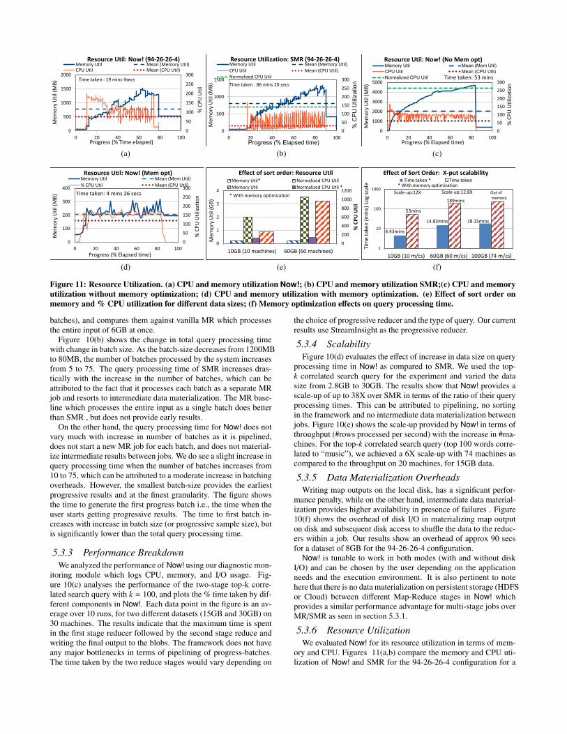
5.3.8 Qualitative EvaluationResult Convergence In order to determine the speed of conver-gence we compute the precision (for the top-k correlated searchquery) of the progressive output values that we get as intermediateresults. Figure 12(a) varies k and plots precision against the numberof progress-batches processed for a data size of 15GB, with a con-figuration of 60-43-43-1 and 200 progress batches. The precisionmetric measures how close progressive results are to the final top-k.We see that precision quickly reaches 90%, after a progress of lessthan 20% as the top k values do not change much after sampling20% of the data (lower k values converge quicker as expected).This shows the utility of early results for real-world queries wherethe results converge very quickly to the final answer after process-ing small amounts of data.Progress Semantics We compare result quality against an MRO-style processing approach using the clicks dataset to compute CTR(Figure 2) progressively. We model variation in processing time us-ing a skew factor that measures how much faster Qi is, as comparedto Qc. A skew of 1 represents the hypothetical case where perfectCTR information is known a priori, and queries follow this relativeprocessing speed. Figure 12(b) shows the % error in CTR esti-mation plotted against % progress. The experiment shows that ifdifferent queries proceed at different speeds, early results withoutuser-defined progress semantics can become inaccurate (althoughall techniques converge to the same final result). We see that evenmoderate skew values can result in significant inaccuracy. On the

0.4

0.6

0.8

1

0 20 40 60 80 100

Pre

cisi

on

% Progress

Top-k Convergence

k-1000 k-500

k-100 k-50

k-10

(a)

0 25 50 75 100

-100

0

100

200

300

400

% Progress (Progressive Output)

% C

TR E

rro

r

CTR Estimation errorNow! MRO (Skew 0.2) MRO (Skew 0.5)

MRO (Skew 2) MRO (Skew 5)

(b)

Figure 12: Qualitative analysis. (a) Top-k Convergence; (b)Error estimation of progressive results.other hand, progress semantics ensure that the data being correlatedalways belongs to the same subset of users, which allows CTR toconverge quickly and reliably, as expected.6. RELATED WORKApproximate Query Processing Online aggregation was orig-inally proposed by Hellerstein et al. [21], where the focus wason grouped aggregation with statistically robust confidence inter-vals based on random sampling. This was extended to handle joinqueries using the ripple join [17] family of operators. Specializedsampling techniques have been widely studied in subsequent years(e.g., see [9, 20, 30]). Laptev et al. [25] propose iteratively com-puting MR jobs on increasing data samples until a desired approx-imation goal is achieved. BlinkDB [2] constructs a large numberof multi-dimensional samples offline using a particular samplingtechnique (stratified sampling) and chooses samples automaticallybased on a user-specified budget.

We follow a different approach: instead of the system takingresponsibility for query accuracy (e.g., as sampling techniques)which may not be possible in general, we involve the query writerin the specification of progress semantics. A query processor usingPrism can support a variety of user-defined progressive samplingschemes; we view prior work described above as part of a layer be-tween our generic progress engine and the user, that helps with theassignment of PIs in a semantically appropriate manner.MR Framework Variants Map-Reduce Online (MRO) [12] sup-ports progressive output by adding pipelining to MR. Early resultsnapshots are produced by reducers, each annotated with a roughprogress estimate based on averaging progress scores from differ-ent map tasks. Unlike our techniques, progress in MRO is an op-erational and non-deterministic metric that cannot be controlled byusers or used to formally correlate progress to query accuracy or tospecific input samples. From a data processing standpoint, unlikeNow!, MRO sorts subsets of data by key and can incur redundantcomputations as reducers repeat aggregations over increasing sub-sets (see [7] for more details).

Li et al. [26] propose scalable one pass analytics (SOPA), wherethey replace sort-merge in MR with a hash based grouping mecha-nism inside the framework. Our focus is on progressive queries,with a goal of establishing and propagating explicit progress in

the platform. Like SOPA, we eliminate sorting in the framework,but leave it to the reducer to process progress-sync ordered data.Streaming engines use efficient hash-based grouping, allowing usto realize similar performance gains as SOPA inside our reducers.Distributed Stream Processing SPEs answer real-time tempo-ral queries over windowed streams of data. We tackle a differentproblem: progressive results for atemporal queries over atempo-ral offline data, and show that our new progress model can in factbe realized by leveraging and re-interpreting the notion of timeused by temporal SPEs. Now! is an MR-style distributed frame-work for progressive queries; it is markedly different from dis-tributed SPEs [1] as it leverages the explicit notion of progress tobuild a batched-sequential data-parallel framework that does nottarget real-time data or low-latency queries. The use of progress-batched files for data movement allows Now! to amortize transfercosts across reducer per-tuple computation cost. Now!’s architec-ture is designed along the lines of MR with extended map and re-duce APIs, and is designed for a Cloud setting.Interactive Full-Data Analytics Dremel [29] and PowerDrill [18]are distributed system for interactive analysis of read-only largecolumnar datasets. Spark [37] provides in-memory data structuresto persist intermediate results in memory, and can be used to in-teractively query big data sets or get medium-latency batchwise re-sults on real-time data [38]. These engines have a different goalfrom us; by fully committing memory and compute resources apriori, they provide full results to queries on hot in-memory data inmilliseconds, for which they use careful techniques such as colum-nar in-memory data organization for the (smaller) subset of datathat needs such interactivity. On the other hand, we provide genericinteractivity over large datasets, in terms of early meaningful re-sults on progressive samples and refining results as more data isprocessed. Based on the early results, users can choose to poten-tially end (or possibly refine) computations once sufficient accuracyor query incorrectness is observed.

7. CONCLUSIONSData scientists typically perform progressive sampling to extract

data for exploratory querying, which provides them user-control,determinism, repeatable semantics, and provenance. However, thelack of system support for such progressive analytics results in atedious and error-prone workflow that precludes the reuse of workacross samples. We proposed a new progress model called Prismthat (1) allows users to communicate progressive samples to thesystem; (2) allows efficient and deterministic query processing oversamples; and yet (3) provides repeatable semantics and provenanceto data scientists. We showed that one can realize this model foratemporal relational queries using an unmodified temporal stream-ing engine, by re-interpreting temporal event fields to denote progress.Based on this model, we built Now!, a new progressive data-parallelcomputation framework for Windows Azure, where progress is un-derstood and propagated as a first-class citizen in the framework.Now! works with StreamInsight to provide progressive SQL sup-port over big data in Azure. Large-scale experiments showed orders-of-magnitude performance gains achieved by our solutions, withoutsacrificing the benefits offered by our underlying progress model.While we have studied the application of Prism to MR-style com-putation, applying it to other computation models (e.g., graphs) isan interesting area of future work.

8. REFERENCES[1] D. Abadi et al. The design of the Borealis stream processing engine.

2005.[2] S. Agarwal et al. Blinkdb: Queries with bounded errors and

bounded response times on very large data. In EuroSys, 2013.

[3] M. Ali et al. Microsoft CEP Server and Online BehavioralTargeting. 2009.

[4] B. Babcock et al. Models and issues in data stream systems. 2002.[5] R. Barga, J. Ekanayake, and W. Lu. Iterative mapreduce research on

Azure. In SC, 2011.[6] R. Barga et al. Consistent streaming through time: A vision for

event stream processing. 2007.[7] B. Chandramouli et al. Scalable progressive analytics on big data in

the cloud. Technical report, MSR. http://aka.ms/Jpe5f5.[8] B. Chandramouli et al. Temporal analytics on big data for web

advertising. In ICDE, 2012.[9] S. Chaudhuri, G. Das, and U. Srivastava. Effective use of block-level

sampling in statistics estimation. In SIGMOD, 2004.[10] S. Chaudhuri et al. On random sampling over joins. In SIGMOD,

1999.[11] D. Cohn et al. Improving generalization with active learning. Mach.

Learn., 15, 1994.[12] T. Condie, N. Conway, P. Alvaro, J. M. Hellerstein, K. Elmeleegy,

and R. Sears. Mapreduce online. In NSDI, 2010.[13] Daytona for Azure. http://aka.ms/unkcbq.[14] J. Dean and S. Ghemawat. Mapreduce: simplified data processing on

large clusters. OSDI’04.[15] A. Doucet, M. Briers, and S. Senecal. Efficient block sampling

strategies for sequential monte carlo methods. Journal ofComputational and Graphical Statistics, 2006.

[16] P. J. Haas and J. M. Hellerstein. Ripple joins for online aggregation.In SIGMOD 1999.

[17] P. J. Haas and J. M. Hellerstein. Join algorithms for onlineaggregation. In IBM Research Report RJ 10126, 1998.

[18] A. Hall, O. Bachmann, R. Bussow, S. Ganceanu, and M. Nunkesser.Processing a trillion cells per mouse click. PVLDB July 2012.

[19] M. Hammad et al. Nile: A query processing engine for data streams.2004.

[20] J. M. Hellerstein and R. Avnur. Informix under control: Online queryprocessing. Data Mining and Knowledge Discovery Journal, 2000.

[21] J. M. Hellerstein, P. J. Haas, and H. J. Wang. Online aggregation. InSIGMOD, 1997.

[22] C. Jensen and R. Snodgrass. Temporal specialization. 1992.[23] C. Jermaine, S. Arumugam, A. Pol, and A. Dobra. Scalable

approximate query processing with the dbo engine. SIGMOD ’07.[24] Y. Kwon et al. Skewtune: mitigating skew in mapreduce

applications. In SIGMOD, 2012.[25] N. Laptev, K. Zeng, and C. Zaniolo. Early accurate results for

advanced analytics on mapreduce. PVLDB 2012.[26] B. Li, E. Mazur, Y. Diao, A. McGregor, and P. J. Shenoy. A platform

for scalable one-pass analytics using mapreduce. In SIGMOD 2011.[27] O. Maron et al. Hoeffding races: Accelerating model selection

search for classification and function approximation. In NIPS, 1993.[28] M. D. McKay et al. Comparison of Three Methods for Selecting

Values of Input Variables in the Analysis of Output from a ComputerCode. Technometrics, 21, 1979.

[29] S. Melnik et al. Dremel: interactive analysis of web-scale datasets.PVLDB 2010.

[30] N. Pansare, V. R. Borkar, C. Jermaine, and T. Condie. Onlineaggregation for large mapreduce jobs. PVLDB, 2011.

[31] V. Raman, B. Raman, and J. M. Hellerstein. Online dynamicreordering for interactive data processing. VLDB ’99.

[32] A. Rowstron et al. Nobody ever got fired for using hadoop on acluster. In HotCDP, 2012.

[33] E. Ryvkina et al. Revision processing in a stream processing engine:A high-level design. In ICDE, 2006.

[34] The LINQ Project. http://aka.ms/rjhi00.[35] P. Upadhyaya, Y. Kwon, and M. Balazinska. A latency and

fault-tolerance optimizer for online parallel query plans. InSIGMOD, 2011.

[36] T. White. Hadoop: The Definitive Guide. 2009.[37] M. Zaharia et al. Resilient distributed datasets: a fault-tolerant

abstraction for in-memory cluster computing. NSDI’12.[38] M. Zaharia et al. Discretized streams: An efficient and fault-tolerant

model for stream processing on large clusters. In HotCloud, 2012.