A DISTRIBUTED POWER MARKET FOR THE SMART GRID
A Thesis
Submitted to the Graduate Faculty
of the
North Dakota State University
of Agriculture and Applied Science
By
Ryan James McCulloch
In Partial Fulfillment
for the Degree of
MASTER OF SCIENCE
Major Department:
Computer Science
July 2012
Fargo, North Dakota

North Dakota State University Graduate School Title
A Distributed Power Market for the Smart Grid
By
Ryan McCulloch
The Supervisory Committee certifies that this disquisition complies with
North Dakota State University’s regulations and meets the accepted
standards for the degree of
MASTER OF SCIENCE
SUPERVISORY COMMITTEE:
Dr. Kendall Nygard
Chair
Dr. Anne Denton
Dr. Saeed Salem
Dr. Limin Zhang
Approved:
7/2/2012
Dr. Kendall Nygard
Date
Department Chair

iii
ABSTRACT
To address the challenges of resource allocation in the Smart Electrical Grid a new
power market is proposed. A distributed and autonomous contract net based market system
in which participants, represented by the agents, engage in two distinct yet interconnected
markets in order to determine resource allocation. Key to this proposed design is the 2
market structure which separates negotiations between consumers and reliable generation
from negotiations between consumers and intermittent energy resources. The first or
primary market operates as a first price sealed bid reverse auction while the second or
secondary market utilizes a uniform price auction. In order to evaluate this new market a
simulator is developed and the market is modeled and tested within it. The results of these
tests indicate that the proposed design is an effective method of allocating electrical grid
resources amongst consumers, generators, and intermittent energy resources with some
feasibility and scalability limitations.

iv
AKNOWLEDGMENTS
I would like to thank a number of people for their support of the development of this
work. First of all I thank my advisor Dr. Nygard and the other members of my committee
Dr. Saeed Salem, Dr. Limin Zhang, and Dr. Anne Denton. I thank all of the members of the
Smart Grid Research group with special thanks to group members Steve BouGhosn, Davin
Loegering, Md. Minhaz Chowhurdy for their continual support throughout the course of my
time at NDSU. I thank the NDSU ACM for distracting me from my thesis work when I
needed it most. Finally I thank my family for encouraging and supporting me all my life.

v
TABLE OF CONTENTS
ABSTRACT ................................................................................................................ iii
AKNOWLEDGMENTS .................................................................................................. iv
LIST OF TABLES ....................................................................................................... vii
LIST OF FIGURES .................................................................................................... viii
I. INTRODUCTION ...................................................................................................... 1
A. Background Information on the Electrical Grid ........................................................ 2
B. Introduction to the Smart Grid .............................................................................. 4
C. Literature Review ................................................................................................ 7
D. Problems and Assumptions ................................................................................. 11
E. Introduction to Design and Simulation ................................................................. 13
II. METHODS ........................................................................................................... 16
A. Design ............................................................................................................. 16
B. Simulation ........................................................................................................ 27
III. RESULTS ........................................................................................................... 50
A. Intermittent Generation Utilization ...................................................................... 50
B. Consumer Demand Response.............................................................................. 55
C. Dynamic Pricing ................................................................................................ 60
D. Integration ....................................................................................................... 66
E. Scalability......................................................................................................... 73
IV. DISCUSSION & CONCLUSION ............................................................................... 75
A. Discussion of Results ......................................................................................... 75
B. Validation ......................................................................................................... 77
C. Advantages and Limitations ................................................................................ 78
D. Implications ..................................................................................................... 80

vi
E. Feasibility ......................................................................................................... 82
F. Future Research ................................................................................................ 83
G. Conclusion ....................................................................................................... 84
VI. REFERENCES ...................................................................................................... 86

vii
LIST OF TABLES
Table Page
1. Intermittent Generation Utilization: Generator Configuration ............................... 51
2. Intermittent Generation Utilization: Consumer Configuration ............................... 51
3. Intermittent Generation Utilization: DER Configuration........................................ 51
4. Intermittent Generation Utilization: Consumer Cost Reduction ............................. 55
5. Consumer Demand Response: Consumer Configuration ...................................... 56
6. Consumer Demand Response: Generator Configuration ...................................... 56
7. Consumer Demand Response: Quadratic Cost Savings ........................................ 58
8. Consumer Demand Response: Off Peak Cost Savings ......................................... 60
9. Dynamic Pricing: Consumer Configuration ......................................................... 60
10. Dynamic Pricing: Quadratic Generator Configuration ........................................... 61
11. Dynamic Pricing: Quadtatric PAR reduction ........................................................ 63
12. Dynamic Pricing: Quadratic Cost Savings .......................................................... 63
13. Dynamic Pricing: Off Peak Consumer Configuration ............................................ 64
14. Dynamic Pricing: Off Peak Generator Configuration ............................................ 64
15. Dynamic Pricing: Off Peak PAR Reduction .......................................................... 66
16. Dynamic Pricing: Off Peak Cost Savings ............................................................ 66
17. Integration: Consumer Configuration ................................................................ 67
18. Integration: Generator Configuration ................................................................ 67
19. Integration: DER Configuration ........................................................................ 67
20. Integration: PAR Reduction ............................................................................. 72
21. Integration: PAR Reduction ............................................................................. 73
22. Scalability: Agent Configuration ....................................................................... 73
23. Scalability: Computer Specification ................................................................... 73
24. Scalability: Execution Time .............................................................................. 74

viii
LIST OF FIGURES
Figure Page
1. Contract Net Negotiation ................................................................................. 20
2. Primary Market Negotiation ............................................................................. 21
3. Primary Market Negotiation Process .................................................................. 23
4. Secondary Market Negotiation ......................................................................... 24
5. Secondary Market Negotiation Process .............................................................. 26
6. Market Interaction .......................................................................................... 27
7. Time Synchronization ..................................................................................... 30
8. Typical Household Consumer Demand............................................................... 32
9. Load Shifting Algorithm ................................................................................... 34
10. Example Consumer Load Shifting ..................................................................... 34
11. Dynamic Pricing Functions ............................................................................... 37
12. Off Peak Pricing Function ................................................................................. 37
13. Quadratic Pricing Function ............................................................................... 38
14. Intermittent Energy Resource Generation .......................................................... 39
15. Main Simulation Window ................................................................................. 41
16. Agent Type Selection Window .......................................................................... 42
17. Agent Configuration Windows .......................................................................... 42
18. Simulation Execution Output............................................................................ 43
19. Agent Management GUI .................................................................................. 44
20. Sniffer Agent Window ..................................................................................... 45
21. Introspector Agent Window ............................................................................. 46
22. ACL Message Details Window ........................................................................... 47
23. Simulation Data Output................................................................................... 49
24. Intermittent Generation Utilization: DER Capapcity and Demand .......................... 52
25. Intermittent Generation Utilization: Generator Offloading .................................... 53

ix
26. Intermittent Generation Utilization: Consumer Cost Reduction ............................. 54
27. Consumer Demand Response: Pricing Functions ................................................. 57
28. Consumer Demand Response: Load Shifting Quadratic ....................................... 57
29. Consumer Demand Response: Load Shifting Off Peak ......................................... 59
30. Dynamic Pricing: Quadratic Generator Loads and Prices ...................................... 61
31. Dynamic Pricing: Quadratic Consumer Load Shifiting .......................................... 62
32. Dynamic Pricing:Off Peak Generator Loads and Prices ......................................... 65
33. Dynamic Pricing: Off Peak Consumer Load Shifting ............................................. 65
34. Integration: Generator Prices........................................................................... 68
35. Integration: Generator Loads ........................................................................... 69
36. Integration: Expensive Gen Consumer Demands ................................................ 69
37. Integration: CheapGen Consumer Demands ...................................................... 70
38. Integration: WindDer Load .............................................................................. 71
39. Integration: SolarDer Load .............................................................................. 71
40. Scalability: Execution Time .............................................................................. 74

1
I. INTRODUCTION
The world runs on electricity. Reliable and omnipresent, modern society could not
exist without it. From the simple act of providing light or heating and cooling homes, to
powering the ever more complex network of communications infrastructure and computers,
electricity is now nearly synonymous with energy. Key to this new age of electricity is the
generation, transmission, and distribution network that supports it, commonly known as the
electrical grid. Unfortunately reliance on electricity has placed an enormous burden on
electrical grid operators. Constant pressure to be powerful, reliable, and above all cheap has
prevented the electrical grid from undergoing the significant upgrades and changes that
must be made in order for it to continue to meet the energy needs of the next century as it
has the last. These upgrades include the introduction of “green” electricity generation
known as distributed energy resources or DERs, as well as computer monitoring and control
technologies. The new electrical grid that could result from the introduction of these
technologies is broadly referred to as the Smart Grid.
This new Smart Grid faces many challenges in its implementation. This paper
addresses the problem of resource allocation through a market based multi agent system in
the Smart Grid. The goal of this research is to design, model and test in simulation a viable
and effective autonomous distributed negotiation system and market for the buying and
selling of electricity between Consumers, Reliable Generators, and Intermittent Energy
Resources such as DERs. In order to achieve this goal a number of objectives must be met
through simulation modeling and testing. The first objective is that it must be determined
whether intermittent energy resources can be integrated and utilized in the system to help
reduce load on main generators and save consumers money. The next objective is that it
must be determined if consumer demand response is an effective and a viable way for
consumers to save money. In conjunction with consumer demand response, it must be
determined if dynamic pricing is a viable and effective method of regulating power usage
while still allowing consumers to save money. The above aspects must then be put together

2
to determine if the integration of all of the disparate systems, operating simultaneously and
cooperatively, can meet needs of all participants effectively. Finally it must be determined if
the representative agents have low enough computational requirements as to be able to run
on integrated computers such as smart meters while still being able to scale upwards to the
large sizes required by the electrical grid.
The proposed market is in essence a distributed and autonomous agent based
contract negotiation system in which participants, represented by the agents, engage in two
distinct yet interconnected markets in order to determine resource allocation. The primary
market is organized as a sealed bid first price reverse auction and deals in day long
contracts from generators able to guarantee reliable power generation over that period. The
secondary market is organized as a uniform price auction and deals in hour long contracts
from intermittent energy resources that generate power inconsistently and wish to be used
opportunistically. Agents representing reliable generation will be responsible for forecasting
future prices and loads as well as providing that information to buyers. Consumer agents in
the primary market select their generators based upon the prices and load schedules
provided to them in an attempt to minimize the cost to meet their demand. Agents
representing intermittent energy resources will attempt to sell all of their available electrical
generation whenever possible. Consumer agents in the secondary market will attempt to
use intermittent energy resources to meet power demand in yet another attempt to
minimize costs. After contract negotiation consumers will further attempt to minimize their
costs by shifting a certain percentage of their load from high cost to low cost periods.
A. Background Information on the Electrical Grid
Ever since Thomas Alva Edison turned on the Pearl Street Generating Station the
world has run on electricity. With his historic work on the incandescent light bulb and his
subsequent design and implementation of an electrical grid system to support said light bulb
Edison has loomed large in the history of the electrical grid. In fact Edison’s influence is

3
perhaps too readily seen in today’s electrical grid infrastructure. The basics of generation,
transmission, and distribution were all present on Pearl Street. Were he to be somehow
transported to the future and able to view our current electrical grid system much of the
equipment and techniques used within it would be quite familiar to him. Other than the
introduction of analog consumer side metering and the obvious increase in scale, little has
changed. Comparing this to how utterly bewildered Alexander Graham Bell, a contemporary
of Edison’s, would feel viewing our current day cellular phone network with telecom
satellites, high speed data networks, and internet based calling illustrates just how little
advancement has occurred in the our electrical system over the past 100+ years.
The modern electrical grid had been called the largest and most complex machine in
the world [1] and yet for all of its complexities, the monitoring and operating of the grid has
changed little over the past 100 years. Current grid operators rely on centralized manually
operated control centers that are often not able to fully monitor or react to changes in the
grid. Monitoring technologies are only sporadically available, with end consumers likely not
being monitored at all. Because of this lack of communication, consumers have no real
ability to participate in grid operations to help lower their costs or to help with load
management of the grid overall. Power markets in the existing grid involve only the Utility
companies and the generator operators.
Controlling the current electrical transmission and distribution systems are the power
Utility companies alongside the Independent System Operators (ISOs). Utilities are
ultimately responsible for their customer area but will coordinate with other Utilities through
their regional ISO. In this way monitoring and control of a subsection of the grid is carried
out by the Utilities but information can be passed on to the ISOs in order to form a larger
picture of grid health and operation. This hierarchical centralized control operates the
current grid effectively but unfortunately, as the grid continues to grow more complex and
as the associated amount of information needed to be collected and analyzed grows, it will

4
become more and more difficult to recognize and respond to situations in the electrical grid
from a central location.
Communication in the existing electrical grid is largely one direction if communication
is occurring at all. Usage information is collected from the customers, oftentimes still by
manually checking the gages outside their homes, which is used by the Utilities for billing
the customer at the end of every month. The Utilities will then also use the usage
information in order to purchase power from generation sources for the next period.
Outages at the consumer end oftentimes need to be communicated through a phone call to
the utility before they are aware of it. This one way communication prevents customers
from being an active participant in the operation of the grid. Without information on the
actual cost of power at any period of time customers are unable to respond to changing grid
conditions and Utilities must absorb the fluctuations in cost.
Currently in the electrical grid the only negotiations for power that occur are between
generator operators and utilities. These negotiations are often carried out through their ISO
in order to coordinate the negotiations and ultimately the transmission of the purchased
power. The most common structure for these negotiations is that of a uniform cost reverse
auction. The Utility requests bids on the demand that it must meet. Each generator bids a
certain amount of power over a period of time and its price (the cost of producing the power
plus whatever profit margin is appropriate) after all of the bids are received the Utility
selects generators starting from the cheapest and ascending until its demand is met but
pays all generators at the amount of the highest bid selected. In this way generators are
incentivized to bid their actual costs of production rather than as high as possible while still
wining the bid.
B. Introduction to the Smart Grid
The electrical grid faces many challenges. Yet even with all of these challenges the
current electrical grid distribution system has achieved a nearly 99% reliability [2]. In the

5
future however new problems will arise. Problems like the dramatic increase in load from
Plug in Hybrid Electric Vehicles (PHEVs) or the increasing proliferation of consumer
electronics. This increased load will bring with it an associated increase in size and
complexity of the grid in order to handle it. Increasing complexity will require better
monitoring and control technologies as well as computer automation. On a basic level
increased load will require new generation sources to meet that load. Unfortunately the
desired renewable sources of energy tend to be in the form of unstable DERs and require
extra effort to properly integrate into the electrical grid. In order to maintain the high level
of reliability that the electrical grid has achieved in the past in the future, changes must be
made. To this end a new Smart Electrical Grid system has been proposed by the US
Department of Energy [3]. A system which not only promotes the distributed generation of
green electrical power through sources such as wind turbines and solar panels, but also
more closely and accurately monitors the grid through the use of devices such as smart
meters and phasor measurement units. These improvements along with advanced
visualization, and artificial intelligence technologies help to manage the electrical grid in a
more efficient and reliable manner.
Central to the new Smart Electrical Grid are the advanced computer monitoring,
communications and control technologies. The proliferation of Smart Meters is a vital
improvement planned for the Smart Grid. Smart Meters allow for two way communication
between utilities and customers. It will allow utilities to build a real time picture of electrical
usage and demand on a household level while also giving consumers access to real time
price information as well as household energy usage. This communication facilitates greater
consumer involvement in the electrical grid and allows consumers to have a better
understanding of their usage patterns. Ultimately it is hoped that it will allow them to find
new ways to save energy and money.
One particularly urgent problem currently facing the grid is the issue of resource
assignment and peak demand. Because the current electrical grid system operates on the

6
principle that power is consumed essentially at the same moment it is generated,
generators must be able to provide whatever amount of power is demanded from them at
the moment it is demanded. The reason this is problematic is that power demand changes
dramatically throughout the course of a day, tending to peak at midday. This peak of
electrical demand places great strain on generators as they must rapidly accommodate this
high demand while also economizing their fuel by lowering their electrical output when
demand is low.
The Smart Meter facilitates the addressing of this problem in the introduction of a
new pricing mechanic called dynamic pricing. Dynamic pricing would allow generators to set
a variable price for electricity based upon the demand and would provide consumers with
the information needed to respond to these changes in price. It is hoped that consumers
would then be more conscious of their energy usage and smooth out the demand curve by
spreading the use of their energy intensive devices, such as laundry machines or
dishwashers, to times in which it is least expensive to use them. In this way dynamic pricing
would allow generators to control their loads by encouraging customers to reduce their
usages during peak period and high prices and encouraging customers to increase usages
during off peak periods and lower prices. Consumers can save money by shifting their
power usages and power providers can encourage a flatter load curve and thus generators
would be able to run more efficiently by maintaining a more stable generation amount.
Working with the Smart Meter on the consumer side are many other important
devices. To go along with the Smart Grid and Smart Meters are smart appliances. These are
appliances such as lights, dishwashers, washing machines, or even home heaters and
coolers that are network connected and sensitive to power prices provided to them by the
Smart Meter. These appliances attempt reduce electricity costs by using power more
effectively and at particularly low priced times. For example a smart dishwasher might be
loaded and set to run but won’t start until 2am when it senses that electricity prices are
lowest. A smart heater or cooler might turn off in the middle of the day when it senses that

7
no one is around and that electricity is at its most expensive. The electricity consumption
controller (ECC) works with these smart appliances to even more efficiently schedule the
usage of power. An ECC can be customized with a particular customer’s routine schedule
and associated electricity demand and then work around that schedule to save money. For
example an ECC might be customized with a particular consumers work schedule and so it
knows to only turn on the water heater an hour before the consumer wakes up and takes a
shower but then to turn off the water heater after they leave in order to save on electricity.
These devices, the smart meter, ECC, and smart appliances, work together to form what is
commonly referred to as a Smart Home.
Outside of the household many monitoring and control devices support the Smart
Grid. Perhaps chief among these devices is the Phasor Measurement Unit or PMU as it is
commonly known. This device measures the phase of the electrical power at a given point in
the electrical grid. This phase information when monitored across the entire grid allows
operators to form a real time measurement of grid health and stability. Running at 60 Hz,
PMU data can be gathered far more quickly than human operators would ever be able to
respond. This combined with the fact that due to its electrical nature situations in the grid
can change at nearly the speed of light has caused many to suggest that computer
automated control be used in the Smart Grid. In this way computer monitors could sense
the state of the grid, analyze it, and respond to it before a fault could occur or propagate.
C. Literature Review
The Smart Grid, while a relatively new topic in computer science, has a wealth of
research behind it. In [3] the basic concepts what the Smart Grid should be are introduced,
including greater consumer choice, distributed generation, and dynamic pricing. In [4] as
well what the Smart Grid should be and could do is analyzed. In a system referred to as
GridWise (as this report predates the term Smart Grid) researchers find that by introducing
among other things more distributed generation as well as encouraging demand response

8
from consumers that over $100 billion of benefit value could be created over the next 20
years. The need and benefit of autonomous control of the grid is described in [5] as well as
in [6]. Simulation also comes to the forefront of Smart Grid development as described in
[7]. The paper concludes that not only can simulation help to develop better design but also
that they can be useful in convincing policy makers to implement changes. [8] also speaks
to the importance of simulation in helping to advance the Smart Grid. Integrating stochastic
or intermittent generation sources into the grid is a difficult proposition and its effects,
specifically with wind power, are analyzed in [9]. They find that systems must either be
highly flexible or be able to very accurately predict generation in order to integrate wind
power without undesirable consequences. In [10] as well, the problems of integrating DERs
or Distributed Generation (DG) as it is referred to in the paper, is studied. Through
simulation they find that changes must be made to the structure of the grid order to
incorporate the stochastic nature of wind power. The communications structure the current
grid and the future Smart Grid is considered in [11]. They find that the current one way flow
of information is unsuitable for Smart Grid operation and that communication between the
consumers and the generators must be facilitated. [12] Also looks at the communications
infrastructure required to facilitate DER integration and demand response. They find that by
connecting the consumers more closely with DERs and with generation in general that
participants can see a nearly 7 percent reduction in costs or increase in profits.
As noted previously, dynamic pricing is one of the most important advancements
proposed with the Smart Grid. In [13] the possible impact in California of multiple dynamic
pricing strategies is analyzed including, peak-time rebate (PTR) and real-time pricing (RTP).
They find that even without automated demand response systems that California could see
as much as $6 billion in benefit. [14] attempts to determine how consumers might respond
to dynamic pricing as well. [15] also looked at the effects of dynamic pricing but this time
with real world experimental evidence from 15 locations. They find that dynamic pricing can
be quite effective with time of use pricing lowering peak loads by up to 6 percent and critical

9
peak pricing lowing peak loads by up to 20 percent. Again the effects of dynamic pricing are
analyzed in [16] this time in Norway. They find that a lowering of over 4% in peak load was
achieved. The introduction of dynamic pricing can cause instability in the power markets
however, which is analyzed by [17]. They find that with certain stabilizing algorithms
dynamic pricing can be used effectively. While most research is in favor of dynamic pricing
[18] does point out some problems. Primarily the author finds that in some residential
markets the cost of infrastructure upgrades to enable dynamic pricing is not offset by the
savings of generators nor the consumers themselves. [19] attempts to address these
problems by recommending that individual consumers form “contract-based … demand
subscription” with generators. As would be expected with dynamic pricing, price forecasting
becomes very important. This issue is discussed by [20], [21], [22] each with their own
unique techniques.
In order to see the greatest benefit from dynamic pricing consumers should be
equipped with an ECC. Much research work has been done on the usage of these devices.
[23] for example takes a look at the scheduling of a water heater throughout the course of
a day. In [24] researchers investigate the possibility of using web technologies to manage
and schedule the use of electricity in the home. Web technologies are also used in [25]
except in this design customers will place orders ahead of time to the Utility companies who
will then organize their resources to best meet the pre purchased demand. Both [26] and
[27] consider the problem of scheduling power usage when the price is unknown or
uncertain. Previous research has focused primarily on communication between the
consumer and the utility company however [28] and [29] consider how consumption
scheduling might be enhanced by communication amongst consumers. Both of them find
significant gains though the incorporation of cross consumer communication. In [30] the
utility is eschewed entirely for direct communication between the consumers and the
generators. They find that this simple bidirectional communication allows for effective
optimization of consumer load scheduling. Putting both of these concepts together, [31] has

10
smart meters communicating both with each other and directly with the generators. They
demonstrate how this allows the generator to control load through pricing adjustments as
well as consumers to optimally shift their loads to minimize costs.
While the current concept of a Smart Grid only extends back to 2005, agent based
markets have existed in research since the 1980’s. The contract net protocol for example as
proposed in [32] laid the ground work for nearly all of the types of agent negotiations that
would follow. Similarly the Belief, Desire, and Intent otherwise known as BDI framework as
presented in [33] establish a structure for agent actions. In [34] the authors discuss the
basics of agent markets and conclude that they are an effective means of resource
allocation and distributed decision making through the use of price controls. The issues of
agent negotiation and interaction are broadly discussed in [35]. Intelligent agents are being
applied to every sort of problem from Stock Trading in [36], to International Crisis’s in [37]
with success. Negotiation formats range from argumentation based as researched in [38] ,
where agents must convince each other of their position, to market and trading based
interaction as discussed in [39]. Market based bidding agents are discussed extensively in
[40] where competitive testing has helped to dramatically advance the field. In [41] specific
bidding strategies are discussed for market agents. The design of a market and a technique
called algorithmic mechanism design is presented in [42]. Essentially they recommend that
when trying to design a market system to achieve globally optimal results you must design
it in such a way that globally optimal behaviors are rewarded on an individual level.
Intelligent agents are core to many of the proposed advancements of the Smart Grid
and have seen a large amount of research interest. In [43], [44], and [45] an agent design
and simulation is proposed for the autonomous control and self-healing of the Smart Grid.
The tools available to researchers to simulate electricity markets are surveyed in [46].
Models for the wholesale electricity market are analyzed in [47] and their testing described
in [48] . The benefits of uniform price auctions over pay-as-bid auction in the wholesale
electricity market are described in [49]. Using an agent based simulation the demand

11
response of commercial buildings is examined in [50]. Another agent simulation, this time
using delegate ants, is proposed and tested for the negotiation between resource agents
and power user agents in [51]. Contract choice in a distribution grid model is analyzed using
an agent simulation in [52]. In [53] a simple negotiation structure based on contracts nets
is proposed and the effects of power contract negotiations between dynamically priced
providers and consumers are examined. A continuous double auction mechanism is used
along with considerations for transmission line capacities and congestion in [54] for their
agent based electricity market simulation.
D. Problems and Assumptions
While there are many challenges and possibilities for research in the proposed Smart
Grid this paper attempt to address the broadly defined problem of resource assignment.
Even within the field of resource assignment in the Smart Grid there are a number of
specific issues considered. Foremost among these issues is the problem of scale and
complexity in the electrical grid. The grid is very complex and exists over an extremely large
area. It is very difficult to centrally control and administer the grid because of this. Another
issue is that unstable sources of generation, such as solar and wind, are difficult to integrate
into existing energy markets and even proposed Smart Grid energy markets. There are
many advantages to be gained from the introduction of dynamic pricing and the resulting
demand response from consumers but bidirectional communication is difficult and there are
privacy concerns to content with. Due to demand response consumers will have unstable
power demands as they attempt to shift consumption about to save money. On the
generators side they will be dealing with consumer’s attempting to minimize cost but
generators will also wish to flatten their load curves. Along with these problems, the system
to deal with all of these problems must be able to operate on very low power computational
hardware and still make decisions quickly as situations in the grid change rapidly.

12
In addressing these problems a number of assumptions have been made. The most
basic assumption is that all power needs must be satisfied every period and that no
participant may experience either a brownout (under powered) or a blackout (no power).
This is the way that current grid operates for the most part. It has also been assumed that
every consumer is equipped with a real time monitoring and communications device, such
as a smart meter, as well as an electricity consumption controller and a representative
negotiating agent, possibly running on either of the above devices. While this is certainly
not the case currently, installation of these devices is growing and this assumption will likely
hold true for the majority of consumers 10 years from today as discussed in [3]. Another
assumption that has made is that every consuming participant will attempt to shift a certain
amount of their load in response to the real time dynamic pricing of their power. This is an
easy assumption to make as a wealth of research has shown this to be true, including [13],
[15], and [16]. It has also been assumed that all contracts enacted between consumers and
generators are unilateral in that the supplier of power promises to provide the requested
amount of power if needed, but the consumer does not promise to consume any certain
amount of power and is free to make secondary opportunistic contracts with other
suppliers/generators. Currently consumer power contracts operate in a similar fashion in
that a consumer is contracted with a Utility but makes no promise to use a certain amount
of power. Whether this assumption will hold true in an actual power market has much to do
with politics and policy and as such is difficult to predict. For the sake of the proposed
design and due to the beneficial effects of this contract type to all parties, this assumption
has been made. One of the more difficult assumptions that must be made is that generators
of power will only bid their marginal cost of production along a specified dynamic pricing
function and will not attempt to maximize profits by over bidding. Power prices are currently
regulated by federal and state governments, in order to ensure that all Americans can afford
power to their homes. This assumption continues that tradition in that it attempts to keep
prices low for the benefit of consumers. Finally, the last and likely largest assumption that is

13
made is that power will be delivered as negotiated. The transmission of electricity is
assumed to be handled by an external entity such as the appropriate ISO or local
transmission owners/operators and is not part of this analysis or simulation. Essentially this
means that if a contract can be made then transmission can and will occur. This assumption
has been made primarily in the interest of keeping the scope of this research contained. The
proposed design concerns how resources in the grid should be allocated, not how they
should be transmitted or distributed. While considerations to the structure of the grid might
alter and improve the allocation process it is a consideration for further research beyond the
scope of this paper.
E. Introduction to Design and Simulation
In order to address the above problems and with the above assumptions, a novel
agent-based power market for allocation of electrical power has been designed. The
cornerstones of the market design are its distributed and autonomous nature, its three
participant types, and its dual market structure. This market design has then been modeled
in a simulation built upon the Java Agent DEvelopment Framework (JADE). This simulation
and testing is carried out to determine a number of key points including: if intermittent
energy resources can be integrated into the system and utilized as best able to reduce load
on main generators and save consumers money; if dynamic pricing is still a viable and
effective method of regulating power usage and flattening the load curve; if consumer
demand response is still a viable way for consumers to save money; if all of the above
systems can be integrated together to work simultaneously and cooperatively; and if all
representative agents have low enough computational requirements as to be able to run on
integrated computers such as smart meters or ECC devices while still allowing the system to
scale upwards appropriately.
The distributed and autonomous nature of the proposed design goes hand in hand.
As established in the previous sections the electrical grid is difficult to control centrally due

14
to its size and complexity. This is why a distributed approach has been chosen for the power
market design. What this means is that every agent is acting in its own interests with no
control being exerted on it from central location. Ideally this means that through the
process of all agents greedily working towards solutions best for themselves that the whole
grid results in an effective and efficient solution. Unfortunately by distributing control each
participant’s responsibilities become more complex. By having each participant represented
by an intelligent agent acting in their interest it takes pressure off of human consumers to
manage their energy needs and related purchasing. Another benefit of autonomous control
is that it can act far more quickly than a human counterpart could. A speed increase which
is desperately needed in the Smart Grid as situations can change at light speed.
The participants in this new power market are broadly placed into three different
categories with each category’s individuals being represented by a different type of agent.
The first category or agent type is the consumer. This agent type represents any participant
that consumes power and wishes to purchase it. The different types of consumers, such as
household, commercial, or industrial, can all be represented by this single agent type. The
next category or type of participant is reliable generation. This category includes any
provider/seller of electricity that is able to generate electricity consistently. This type of
agent could represent generator types such as oil, coal, or nuclear. The final participant
category is, in contrast to the previous type, intermittent energy resources or in general
most types of DER. What this basically means is that any source of electrical power that is
only able to provide electricity intermittently or unreliably would be represented by this
agent type. Generators such as wind or solar would fit into this category.
Key to this entire proposed design is the dual market structure based on the three
participant types. The primary or reliable generation market is where consumer agents
negotiate power contracts with reliable generator agents. This market operates as a sealed
bid first price reverse auction. The contracts made in this market are relatively long, 24
hours long. This is also the market where the dynamic pricing of power plays the largest

15
role. The secondary or intermittent energy resource market is where consumer agents
negotiate power contracts with intermittent energy resource agents. Because intermittent
energy resources are unstable in their energy production they require a different market
mechanism to integrate them. This market operates as a uniform price auction. The
contracts in this market are relatively short, only an hour long, in order to accommodate the
unpredictability of DER generation. These two markets do not exist in isolation however.
They interact in primarily two ways. The primary market raises the price for the secondary
market and through the lowering of the primary market’s load the secondary market lowers
the price of the first.
The above design is novel in comparison to similar research such as [51], [52], [53],
and [54] in a number of ways. First of all, the dual market structure used to address DER
generation instability is unique to this design. The use of load and price curve (that is data
values over time) in the negotiation processes rather than simply individual time of use
values is also unique. The inclusion of many generators for contract choice decisions along
with the incorporating the demand response of consumers into the simulation is unique to
this design. The lack of any central authority or decision maker in the design is rare for
Smart Grid resource allocation. This design’s ability to facilitate consumer demand response
while still maintaining consumer privacy is unique among the reviewed research. The
customizability of the market simulation is extensive. Things such as time granularity,
typical consumer load profiles, load shifting parameters, DER generation profiles, and
traditional generation pricing functions are just a few of the things that can be customized
and altered in the simulation. This is rare for a novel market design. Overall this design is
novel in a number of ways and in general should facilitate further discussion and testing of
alternate power market designs and solutions.

16
II. METHODS
A. Design
While the previous sections briefly discussed the main points of the power market
design, in this section the design and the decisions behind it will be discussed in detail. First
the distributed and autonomous agent based nature of the market will be discussed. Then
each of the participant types will be further elaborated upon. Finally an in depth look will be
taken at the dual market structure and the rationale behind it. The basic contract net
structure as well as each of the markets themselves will be examined.
The distributed nature of agents is precisely why they were chosen for this design.
As described in the introduction, the Smart Grid is far too large and complex to ever be
centrally controlled. By distributing agents across the grid the large problems of operating
electrical grid can be broken down and worked on by many cooperative agents
simultaneously. By simply designing the market in such a way that each agent’s ideal
solution coincides with the global ideal solution global problems can be solved far more
easily than from a central decision making body. It was important for this market design
agents were able to operate entirely independently from one another. That is to say that
there would be no centrally located management agent or controlling authority. By keeping
the agent design distributed in this way the market is able to remain extremely flexible and
resilient. A problem with any single agent does not greatly affect the status of the market as
a whole. Agents can come and go without as they please and the market will still be able to
operate.
That intelligent agents could autonomously operate was also of great importance to
this design. Situations in the electrical grid can change at the speed of light; because of this
participants need to be able to react just as fast. This would be nearly impossible for a
human operator and so computer operated agents are used. Even if human control was
effective the amount of information that must be possessed and the decision making that
must be done would be bothersome for the average household consumer. By using

17
autonomous intelligent agents consumers can see the benefit of advanced electricity market
participation without the hassle manually controlling every negotiation. Consideration must
be taken however, of the complexity of the autonomous agents. Even moderately complex
decision making or market interaction could dramatically slow the agent down as it must
operate on fairly limited embedded computing hardware within say the smart meters
themselves or within the ECC of the home.
As noted above, there are a number of reasons to use software agents in an
electricity market. In this design there are three different types of participants and each of
them are represented in the market by a different type of software agent. The agents will
then participate in the market, negotiating in the interest of the entity they represent.
Consumers need to satisfy their demand but wish to spend as little as possible. Reliable
Generators, as their name indicates, reliably generate power but wishes to control their
loads in a number of ways. DERs intermittently generate power but wish to be used to their
fullest whenever possible. In the end the agents representing these three types of
participants must negotiate in order to satisfy their needs and wants.
Participants of the consumer type make up the majority of entities involved in this
electricity market. They are everything from individual households to commercial buildings
to industrial and manufacturing locations. Essentially any entity in the electrical grid that
has a power demand that needs to be met is represented by a consumer agent. As noted
above consumers need to satisfy their demand first and foremost but along with that
consumer wish to minimize their costs. They primarily do this by intelligently selecting
energy providers based on their prices. Along with this however consumer agents will
attempt to shift a percentage of their total demand from high cost times of the day to low
cost times of the day. This usually involves things like starting the dishwasher at 2am rather
than right after supper. It is in this load shifting or scheduling that the Electricity
Consumption Controller comes into play. The agent representing a consumer will negotiate

18
for a power contract and will use the information gained through these negotiations to
schedule power usage through the Electricity Consumption Controller.
Reliable generators are those generators that produce electricity reliably. There
tends to only be a few of these present in any given market as they are generally large
generating facilities in central locations. The defining attribute for reliable generators is their
ability to guarantee generation capacity for the length of a long term contract (typically 24
hours). The fundamental goal of a generator is to sell electricity but generators also which
to control their load curve. Generator operators want the load curve to be as flat is possible
because this allows them to run the generators more efficiently. What this means is that
generators wish to reduce the peak to average load ratio (PAR) which is the ratio of the
peak load amount place on a generator over the average load. The way that they do this is
through the dynamic pricing of their electricity. The basic principle is that generators raise
the price of electricity when demand is high and lower the price when demand is low. In this
way they encourage consumers to demand less during peak periods and demand more
during off peak periods thus flattening the load/demand curve. In this way generators
attempt to maximize their profits, it should be noted however that in this design that
generators are restricted from biding a base power price above their utility costs. If this
were not done generators would simply bid as high as consumers would still pay and
considering how essential electrical power is to modern life consumers would be willing to
pay quite a bit. This restriction is similar to the way that power prices are currently
regulated by federal, state, and local government.
Intermittent Energy Resources are a category of generators defined in this design to
be those generators which are only able to produce power intermittently. Solar panels and
wind turbines fall into this category or participants. Because they only generate power
intermittently and tend to be both more numerous and smaller in capacity intermittent
Energy Resources must be handled differently than other forms of generation. In general
the primary goal of an intermittent energy resource is to sell all of its available power

19
whenever it is able. Because they cannot be relied upon for consistent energy generation
they are best used opportunistically and in supplement to reliable generation sources for
consumer demand.
The double market structure of this design is one of its primary innovations. By
separating the traditional or reliable generators and the intermittent energy resources both
can be used more effectively. By using the established contract net protocol all agents are
able to communicate with each other in simple and effective manner. The separate markets
allow for separate unique auction styles to be applied on top of the contract net where
appropriate. Having the consumer agents participate in both markets connects them and
allows them to interact with each other indirectly through the consumers.
The contract net protocol is a simple and effective structure for contract negotiation.
It is based on procurement process used by the United State Government and many other
entities for procurement of goods or services. A simple description of its operation, as
shown in figure 1 below, follows. First a consumer will send out a call for proposals (CFP) to
any potential providers. Then any provider that can meet the consumer’s demands will send
back their proposal detailing their ability to meet the consumer’s demands and their price to
do so. After receiving all of the proposals the consumers will then select the proposal that
fulfills their demands at the lowest price and informs the provider that they wish to enter
into a contract with them with the proposed terms. If the provider confirms the contract
then the negotiation is finished and the contract is signed. If the provider rejects the
contract then the whole process begins again. There are two main reasons why I’ve chosen
this method of agent negotiation. First of all, as you can see above and below, it is a very
simple form of negotiation. This is to its benefit as both efficiency in messaging and
computation are needed for the distributed decision making that must take place in this
design. Second of all this method of negotiation has a long history of use by entities of all
types that wish to ensure that purchasing and procurement of goods and services is being
done correctly. This history of use means that this method of contract negation has been

20
well tested and, as evidenced in its continued use today, has been found to be extremely
reliable, efficient and effective.
Figure 1 - Contract Net Negotiation
Building upon the groundwork set by the contract net protocol, the primary market,
aka the reliable generation market, coordinates negotiations between consumer agents and
reliable generation agents. Placed on top of the standard contract net negotiation is a first
price sealed bid reverse auction. To understand what this means it is best to break this
auction down into its parts. The ‘first price’ part of its name refers to the fact that the best
bid price, in this case the lowest, is the price that is paid to the winning bidder. The ‘sealed
bid’ portion of this auction means that bidders have no knowledge of each other’s bids. This
means that there is no advantage or disadvantage to being the first or last person to bid.
Lastly, the ‘reverse auction’ portion of the name refers to the fact that in this style of
auction the providers are the ones bidding on the consumers. While this is normal for a
contract net it is unusual for an auction which usually features consumers bidding on
providers. There are two main reasons this particular auction mechanism has been selected
for the primary market. First of all it gives the generators the power of setting the price for
electricity. This makes sense as not only do generators have a great interesting in
controlling the usage of electricity through its prices but also because generators have the
best knowledge of the actual costs to produce the electricity and are thus better prepared to
set reasonable prices. Secondly having the generators bid on the consumers places the

21
power of contract choice in consumer hands. This encourages competition between the
generators and helps to keep the price down as well as allows consumers to better react to
electricity prices in the form of load shifting. Another key characteristic of the primary
market is that it features long term day long contracts. The reason for this is that having a
longer term contract enables easier usage scheduling by consumers. In making a day long
contract the generator must make predictions as to expected loads and in turn the prices
Figure 2 - Primary Market Negotiation

22
those loads create over period of the contract. This information is relayed to consumers in
the form of price curves included with the bids. Having a day long price curve allows
consumers to proactively schedule power usages. The day long length was chosen because
it represents the smallest amount of time that cyclical consumer load patterns can be seen.
A week or a month could also be used but by having a shorter period of time allows
consumers to react more quickly and often to changing grid conditions. The step by step
process of a single negotiation between one consumer and one generator is shown in figure
2 above.
Figure 3 below illustrates the primary market negotiation process between two
generators (G1 and G2) and three consumers (A, B, and C). This process is presented as a
time series below in a step by step fashion though it should be noted that all of these steps
take place within a single simulated time period. Starting frame 1 in the upper left of the
figure below, the three consumers each send out CFPs to both of the generators in the
system. In frame 2, the two generators respond to the CFPs with proposals to the
consumers. Frame 3 shows that all three consumers have selected G1 as the best proposed
offer and send accepts to that generator. Frame 4 shows generator G1 confirming the
contracts with consumers A and B but then Disconfirming the contract with C. This is
because, as noted in figure 3 above, the generator G1 has recalculated its price curve and
found it to be dramatically different than its initial quote to consumer C due to the two new
contracts made with consumers A and B. In frame 5 after receiving the Disconfirm
consumer C restarts the negotiation process by sending out a CFP to both of the generators.
In frame 6 the generators once again respond to the CFP with proposals. Now in frame 7,
due to the change in prices caused by the two new contracts for G1, G2 now has the best
offer and is selected by consumer C to provide power. Having no other contracts G2
confirms the contract with consumer C in frame 8 and the resource allocation for this period
is finished.

23
Figure 3 - Primary Market Negotiation Process
The secondary market, aka the DER market, also builds on the contract net protocol
foundation. This market facilitates negotiation between consumer agents and DER agents. It
utilizes a uniform price auction structure overlaid on the standard contract net negotiation.
A uniform price auction is one in which a provider wishes to sell their entire stock of a
certain good. The way it works is that a provider initiates the contract net processes and
receives bids for an amount of goods at a certain price. The provider then selects those bids
starting from the highest price and continuing downward according to price until all of their
stock is sold. The provider then sets the price for all of the goods at the price of the first

24
unselected bid. This final price is called the market clearing price, or MCP, as it is the price
at which all goods in stock will be sold. This is ideal for the DER market for two reasons.
Firstly it encourages full usage of DER resources. DERs like wind turbines and solar panels
tend to have a very low cost of operation but owners and operators still wish to maximize
their profit. By allowing DER agents to set their prices just low enough to sell their entire
capacity it keeps prices profitable for operators but still beneficial for consumers. Secondly
this auction structure ensures that those willing to pay the most for electricity are preferred
in contract negotiations. As the price a consumer is willing to pay for DER contract is set by
the price they are currently paying for reliable generation. This means that those consumers
currently paying the most for their electricity will have the best chance of having their prices
Figure 4 - Secondary Market Negotiation

25
lowered by DER usage. One of the most important features of the secondary market is that
the contracts that are negotiated within it are short term usually only an hour. This allows
unstable and intermittent generations sources such as wind and solar to be utilized
effectively. It does this by encouraging opportunistic usage as supplement to a reliable
generation contract rather than dependence on an unpredictable power source. What this
means for the contract net negotiation is that, unlike in the primary market, only single time
of use values such as demand amount and price are passed back and forth. A detailed step
by step illustration of the negotiation process between one consumer and one DER can be
seen above in figure 4.
Figure 5 below shows the step by step process of negotiation in the secondary
market between two DERs (D1 and D2) and three consumers (A,B, and C). Again like figure
4 above while this negotiation is presented in a step by step fashion it actually all occurs in
real-time within a single simulated time period. In frame 1 in the upper lefthand corner of
the figure below the DERs D1 and D2 send out CFPs to all of the consumers in the system.
In Frame 2 the consumers A, B, and C respond to that CFP with proposals. In frame 3 the
DERs both select the best proposals (as described in figure 4 above) and send the selected
consumers an Accpet. In frame 4 The selected consumers confirm their contracts with DER
D1 while consumer A disconfirms its contract with DER D2. This happens because, as
outlined in the figure above consumers will only confirm a contract with a DER if they have
demand not already met by a provider in the secondary market. After confirming a contract
with DER D1, consumer A has all of its demand met already and thus Disconfirms the
contract with D2. Because at the end of a negotiation D2 still has unsold capacity it restarts
negotiations and sends out another CFP to consumers in Frame 5. In frame 6 the consumers
with unmet secondary market demand send proposal back to D2. Not indicated in the below
figure is the fact that athough B’s contract with D1 was confirmed B’s demand was only
partially fufilled and thus it continues bidding. In frame 7 because of consumer B’s
decreased demand D2 is now able to select two customers to sell power to and sends accept

26
messages to both of them. Finally in frame 8 both customers confirm their contrat with DER
D2 and enter into contracts with it.
Figure 5 - Secondary Market Negotiation Process
As noted previously while these two markets do operate separately and
simultaneously but they do not exist in isolation from each other. Through the common
participation of the consumer agents the markets affect each other in a number of ways.
Consumers use the prices they receive in their negotiations in the primary market to
determine how much they will bid into the secondary. In this way high price generation in
the primary market both encourages reduced usage and increases likelihood of DER

27
offloading. This also means that consumers will usually secure a contract in the primary
market before bidding on contracts in the secondary. Another interaction occurs through the
noted DER offloading. All generation in the secondary market takes demand off of primary
market and thus reducing primary market prices. In this way the three participant types and
two markets help to stabilize each other as shown in figure 6 below.
Figure 6 - Market Interaction
B. Simulation
In order to test the above market design, a simulation was developed using the Java
Agent DEvelopment Framework otherwise known as JADE. Because much of the
groundwork for an agent based system is already provided by JADE, focus was primarily
placed on the implementation of the agents themselves. However, as JADE’s agent design
has a large impact on the simulation of the proposed power market design it is worthwhile
to examine its structure as broadly described in [55].

28
As its name implies, JADE is primarily an intelligent agent platform. Fundamentally,
JADE provides the basic structure of an agent; its threaded execution, its behaviors, and its
communication with other agents. In this way all that a programmer must do is decide what
the agents must do rather than how they should do it. For example, what should an agent
do when it receives a certain message, not how should an agent receive messages. Along
with this JADE provides the environment for agent operation. Multiple agents can be run on
the same system or on multiple systems networked together allowing the agents to be
mobile as well as hardware independent.
JADE structures its agents around a variety of behaviors classes. Essentially the
structure and flow of all JADE agent actions are controlled by the types of behaviors
implemented in that agent. For example, the SimpleBehavior class simply performs its
defined action and terminates, but if several SimpleBehavior classes are added as sub
behaviors to a ParallelBehavior then each SimpleBehavior will have its actions performed
simultaneously. Similarly if several SimpleBehavior sub behaviors are added to a
SequentialBehavior then each SimpleBehavior will perform its action one after another.
With these provided behaviors, along with a handful of others, JADE provides programmers
a way to easily create complex agent behaviors.
Along with this behavior structure JADE also provides for agent communication in the
form of Foundation for Intelligent Physical Agents aka FIPA compliant messages. These
messages function very similarly to an email system with each message having a sender,
receiver, message content, and even a subject of sorts known as a performative. Along with
these standard email attributes JADE messages also contain an important piece of
information known as the conversation ID which allows agents to track conversations across
large spans of time and across many messages. These various attributes, besides being
useful in and of themselves, also allow agents to filter their “inbox” or message queue in
order to deal with only the messages they are concerned with.

29
While the agent communication system is quite robust agents need a way to find other
agent to communicate with. To this end, JADE provides two facilities, the agent
management service (ams) and the directory facilitator (df). The agent management service
is a manager for all the agents in the system. Through the ams, agents can acquire a listing
of every other agent within the system. More useful in general (and utilized by this
simulation) is the directory facilitator which functions very similarly to the yellow pages
section of a phonebook. The directory facilitator allows agents to register themselves along
with information on the particular services they offer. In this way agents that require a
service, such as consumers requiring power, can simply ask the directory facilitator for a
listing of agents offering that service. While this does centralize agent communication
somewhat there is efficiency gains in not having to search through or send messages to the
entire agent list.
With all of the provided functionalities described above, JADE is well suited for the
implementation of the proposed contract net negotiation system. Behaviors are in place to
handle simultaneous negotiations. A communication system is provided which allows for the
traditional back and forth communication style of contract negotiation as well as the
tracking of and differentiation between specific conversations. A directory service is even
provided which allows energy providers such as DER or generators to advertise their
available energy to potential consumers. JADE is well equipped for the simulation of this
market design.
With JADE providing the fundamental agent structure for the market design another
important consideration is the simulation of time. An hour granularity was chosen due to the
majority of power system data being available at that granularity. However, the granularity
was implemented in such a way as to make it configurable. One particularly important
assumption in regards to time is that all consumer needs must be met every period.
Essentially this means that no consumer is able to undergo a blackout (no power) or a
brownout (under powered). This also means that negotiations must continue until all

30
consumer needs are met. In order to reflect this assumption in the simulation of time, a
time management agent was created. This time management agent monitors the agents in
the system and keeps the time synchronized among all of them. It does this by only
advancing the current time unit when all agents have ended negotiations. This action is
illustrated in figure 7 below. Agents A, B, and C send messages to the Time management
agent T when they have finished negotiations. Once Time management agent T has
received “satisfied” messages from all participant agents it advances the time one unit and
sends the updated time value to all agents simultaneously at which point the process begins
again. This method of time simulation means that negotiations essentially happen in real
time within a single time unit, in this case an hour. When all negotiations are finished, that
is to say when all consumers are satisfied, the time unit advances and the next time
period’s negotiations begin. In this way the simultaneous and rapid nature of negotiations is
simulated while still allowing for the manual control of time, such as stepping one unit at a
time, as well as for long periods of time to be simulated quickly.
Figure 7 - Time Synchronization
The simulation of the participants themselves was the most challenging part of the
simulation. This is due to the fact that the market design and every action within it is
initiated and operated by the participant agents. Because of this it is worth examining the

31
implementation of the agents designs described above. The three agents types consumers,
reliable generators, and intermittent energy resources will be examined in turn below.
The Consumer agent is implemented into the simulation as a JADE agent named
ConAgent. As noted previously these broad participant types serve to help direct an agent’s
actions in the market but there is still a significant amount of variation that can occur
among agents of the same type. For example the ConAgent allows for the parameters of
demand curve, shift-ability, and minimum shift to be set upon creation of an agent. The
demand curve of a ConAgent is probably its most important feature. The demand curve is
the typical usage pattern of a consumer over the course of a day or, to put it another way,
the usage pattern of the consumer if they were not sensitive to price fluctuations. A couple
of examples of this sort of curve are shown in figure 8. By configuring this demand curve a
variety of consumer types can be simulated such as household, commercial, and industrial.
From this demand curve contracts are negotiated and load shifting is performed. Shift-
ability, next parameter of a ConAgent, is also very important to its operation. A ConAgent’s
shift-ability determines the percentage of total power demand over the course of a day that
a consumer is willing to move from one period of time to another in order to save money.
Essentially this parameter ranges from 0 to 1 and the higher it is the more the consumer
will shift its power usage pattern about. Finally the last configurable parameter of a
ConAgent is the minimum shift amount. This value represents the smallest amount of power
that a consumer will shift from one time period to another. This parameter helps to simulate
the kinds of devices that might be shifted about. For example a high minimum shift value
might mean that only large appliances were being shifted and the new load curve would
reflect that by showing large blocks of power usages moving from certain periods to others.
In practice what this means is that the higher minimum shift is the blocker the shifted load
curve will be while conversely, the lower minimum shift is the smoother the shifted load
curve will be.

32
Figure 8 - Typical Household Consumer Demand
The implementation of ConAgent follows the description of the consumer agent in the
previous design section precisely. If the ConAgent’s current demand for power exceeds the
amount it is being provided then it enters negotiations in the primary market. It does this
by first requesting a list of all registered generators from the df agent and then sends them
all a call for proposals (CFP) message. This CFP initiates the negotiation process illustrated
in figure 2 above. For each recipient of the CFP the ConAgent creates a dedicated parallel
behavior to wait for that generator’s response. Each response is tested against the currently
selected best proposal and if better chosen to replace it. Once all of the generators have
responded with either a proposal or a no bid message the best proposal is used to load shift
against, as described below, and an accept-proposal message is sent to the selected
generator. The ConAgent then waits for a reply. If the reply message confirms the contract
then the contract is enacted then the ConAgent has its demand met and leaves the primary
0
0.5
1
1.5
2
2.5
3
1 2 3 4 5 6 7 8 9 101112131415161718192021222324
Dem
an
d (
kw
h)
Time (Hour)
Typical Household Consumer Demand
Summer
Winter

33
market until time is advanced. If the reply message disconfirms the contract then the
ConAgent restarts negotiations. Simultaneously with this process the ConAgent is constantly
watching out for CFPs from DerAgents representing intermittent energy resources. If
ConAgent receives a CFP it initiates the negotiations illustrated in figure 4 above. Upon
receiving a CFP message the ConAgent initiates a dedicated behavior for that negotiation. If
the DerAgent is cheaper than the ConAgent’s current primary generation source and the
ConAgent has demand unmet by another DerAgent then it will respond to the CFP with a
proposal. The behavior then waits for a reply from the initiating DerAgent. If the DerAgent
replies with an accept-proposal then the ConAgent checks to see if it still have unmet
demand and if so replies to the DerAgent with a confirm message. If the DerAgent replies
with a reject-proposal message then the behavior is killed.
The load shifting or the demand response of consumers is an important part of the
power market design and as such is an important part of the implementation of the
ConAgent. As discussed previously the primary goal for consumers in shifting their load is to
save money. A simple and novel method of achieving this goal has been implemented in the
ConAgent. Below in figure 9 is the psudocode for the load shifting algorithm. It starts by
calculating a cost curve (CostArray below) through the use of a weighted product model. It
does this by multiplying the values of the demand curve (LoadArray below) by the values of
the price curve (PriceArray below) weighting the price curve more heavily through its
exponent. This weighting is done to reflect the greater concern consumers have for cost
savings than for load flattening. The chosen weighting amounts were chosen after a very
simple set of testing and in no way reflect the optimal values. The algorithm then attempts
to minimize this cost curve by iteratively moving the minimum shift amount of power
(ShiftMin below) from the highest cost period to the lowest cost period. It does this until it
has moved the shift total amount of power (TotalShift below) a parameter calculated by
multiplying the total daily load by the shift-ability parameter discussed above.

34
Figure 9 - Load Shifting Algorithm
In shifting load this way a consumer takes into account both the price of electricity
at each point and time as well as their demand. This encourages them to flatten their
demand curve along with moving their usage away from high cost periods. While the effects
of this shifting will be examined in detail in the experimental results of the simulation a
simple example of the results of this load shift algorithm in action are displayed in figure 10
below.
Figure 10 - Example Consumer Load Shifting
0
0.5
1
1.5
2
2.5
0 6 12 18
Lo
ad
(kw
h)
Time (Hour)
Load Shifting in Consumers
Shifted
Original

35
Similar to the ConAgent the reliable generator participants are represented by agents
implemented into the JADE simulation as GenAgent. This agent also has a number of
configurable parameters that allow this broadly defined participant type to represent many
different individuals. The parameters include; capacity, base price, and the dynamic pricing
function. Capacity refers to the maximum amount of energy that this generator can produce
at any giving point in time. It is assumed that because these are reliable generators that
this capacity amount is a constant across all periods of time. This means that reliable
generators are able to produce up to a certain amount of power no matter what time of day
it is or what the conditions are. The base price parameter is the minimum amount of money
that the generator will charge for electricity per kWh. This base price represents the cost of
producing energy through the generator. Charging less than the base price would mean that
it costs the generator more to produce the energy than they are making selling it and thus
they would lose money on every kWh sold. The dynamic pricing function determines how
the demand for electricity is related to the price the generator charges for it. The dynamic
pricing function must take in demand (or current load on the generator) and base price and
then output the price that will be charged to contracted consumers.
The GenAgent is implemented in accordance with the design for reliable generation
agents described above in the design section. A GenAgent simply waits to receive one of
three types of messages: Time update, Contract Termination, and CFP. When a time update
message is received GenAgent simply updates its values and replies with a satisfied
message to the TimeAgent. When a Contract Termination message is received GenAgent
simply removes the specified contract from its records. A CFP message is what initiates the
negotiation illustrated in figure 2. Upon receiving a CFP the GenAgent starts a dedicated
behavior to handle the negotiation. If the GenAgent has available capacity to meet the
demand of the CFP then the GenAgent calculates a price curve based upon the provided
demand curve and its current total load curve and sends it back to the ConAgent from which
the CFP originated. The negotiation behavior then waits for a reply from the ConAgent. If

36
the GenAgent receives an accept-proposal then the GenAgent rechecks its available capacity
to ensure that it can still meet the demand and it calculates and then compares the new
price curve to the old price curve to ensure that its prices have not significantly changed
since the beginning of the negotiation. If everything checks out then GenAgent replies with
a confirm message and enacts the contract. If something does not check out then the
GenAgent replies with a disconfirm message and kills the behavior. If the generator receives
a reject-proposal then the behavior is killed.
Because the dynamic pricing function plays such a large role in the negotiations and
in the demand response of consumers it is worthwhile to examine it further. Outside of a
flat price for electricity there are two main methods of dynamic pricing. The first one, off-
peak pricing, establishes two prices for electricity and an off-peak threshold. When the
demand for electricity is below the off-peak threshold the price is set to a lower off-peak
amount. When the demand for electricity rises above the off-peak threshold the price is set
to the dramatically higher peak amount. The primary advantage of this model of dynamic
pricing is its simplicity. Off-peak periods tend to be fairly consistent from day to day and so
consumers are able to easily alter their demand without the need for real-time price
monitoring tools. The second function, real time pricing (RTP), uses a continuous function to
set the price for electricity every period based on the current demand on the supplying
generator. Essentially what this means is that as demand goes up so too does price. This
model of dynamic pricing allows generators to more carefully control the price and by
extension the demand for electricity. The major problem of RTP however is that because of
the continuous changes in the price for electricity consumers require technological
assistance to appropriately respond. figure 11 below illustrates the basic curve of these
pricing functions.

37
Figure 11 - Dynamic Pricing Functions
In the simulator these pricing functions have been implemented fairly simply. The
psudocode for off-peak pricing can be seen in figure 12 below. In this example the threshold
has been set to half of the capacity. When the demand is less than half of the total capacity
of a generator the price for power is set equal to the base price of that generator. When the
demand is equal to or greater than the capacity however the price is set to the multiple of
the base price. As is likely apparent in figure 11 the base price was 0.1 and the capacity
was 40.
Figure 12 - Off Peak Pricing Function
For RTP a similarly simple implementation was used. Research in [13], [17], and
[31] all indicate that quadratic functions are most appropriate for RTP, thus, as can be seen
in the psudocode of figure 13, that is what has been implement. In the psudocode below,
some important factors have been chosen for the quadratic function. Capacity helps to
0
0.2
0.4
0.6
0.8
1
1.2
1.4
1.6
1.8
2
1 6 11 16 21 26 31 36
Pric
e (
$/
kW
h)
Demand (kWh)
Dynamic Pricing Function Comparison
Quadratic
Off-Peak

38
control the rate at which prices change due to shifts in demand. For the most part, capacity
changes with the number of participants in the system. With a small number of participants
a greater variability in price caused by a high ScaleFactor allows for more dynamic
interaction between generators and consumers. On the other hand, with a large number of
participants the price can vary too dramatically and the ScaleFactor must be reduced to
keep the prices for electricity within a reasonable range. BasePrice is used as a factor
throughout the function in order to increase its influence on the resulting price. This means
that generators with a low base price (which indicates a low cost of production) will continue
to generally have a lower dynamic price than those with a high base price. By incorporating
base price more fully into the calculation of the dynamic price it further encourages the use
of efficient generators.
Figure 13 - Quadratic Pricing Function
The intermittent generation participant’s agents follow suit with the others and are
implement into a JADE agent called DerAgent. Once again the parameters of DerAgent allow
it to represent a wide variety of individuals that could all be classified under the intermittent
generation type. DerAgent parameters include base price and capacity curve. Like GenAgent
before it DerAgent also features a base price parameter that indicates the minimum price
that the DER will offer electricity for. Unlike GenAgent, DerAgent does not use this base
price parameter to directly set its price. As discussed in the design section above the
secondary market sets its prices through a uniform cost auction and in the auction base
price is as simply the lowest price that a DerAgent will go to reach a market clearing price.
The other parameter of an individual DerAgent is the capacity curve. This parameter
determines the generation capacity of a DerAgent every period and is responsible for
simulating the intermittent nature of intermittent generation. In order to accurately model

39
generators such as solar panels and wind turbines, historical data was gathered from [56]
and [57]. This data was then used to create three month long csv files representing a
particular wind turbine or solar panels generation at every hour over that period of time.
Figure 14 below displays a particular week of data from one of these files. By representing
DER generation in this way the intermittent nature of those types of generators is
maintained along with the natural shapes of their generation curves. This method of
simulation also avoids the problems of attempting to mathematically model an essentially
chaotic system.
Figure 14 - Intermittent Energy Resource Generation
The implementation of DerAgent follows the description of the intermittent energy
resource agent in the previous design section precisely. If the DerAgent’s current generation
capacity exceeds the amount it is providing to ConAgents then it enters negotiations in the
secondary market. It does this by first requesting a list of all registered consumers from the

40
df agent and then sends them all a call for proposals (CFP) message. This CFP initiates the
negotiation process illustrated in figure 4 above. For each recipient of the CFP the DerAgent
creates a dedicated parallel behavior to wait for that ConAgent’s response. Once all of the
consumers have responded with either a proposal or a no bid message proposals are
selected by sorting all of the proposals by cost descending and selecting proposals from the
top until either all of the generation capacity is allocated or the bid price drops below the
DerAgent’s base price. An accept-proposal message is sent to each of the selected
proposal’s ConAgents. For each accept-propsal recipient the DerAgent creates a dedicated
parallel behavior to wait for that ConAgent’s response. If a reply message confirms the
contract then the contract is enacted. If a reply message disconfirms the contract then that
behavior is killed. Once all receiver behaviors have finished if the DerAgent has any unsold
capacity it restarts negotiations otherwise it waits until time is advanced.
The simulation application itself is fairly simple from user point of view, yet still bears
examination. The application fulfills three primary purposes; the configuration of a
simulation environment and its participants, the execution and high level monitoring of a
undergoing simulation, and the outputting of detailed simulation data for further analysis.
To begin with though, an overview of the GUI is in order. Below in figure 15 is the main
window of the application. Taking up the center of the screen is a large text box that will be
outputting status messages from them participant agents during execution. Below that
window, in bold, is the current time period given as number of hours since the start of the
simulation. For example having simulation 2 days the current time would read 48. Below the
current time value are four buttons; Add Agent, Pause, Play, and Step. Pause, Play, and
Step all control the execution of the simulation itself. Step advances the simulation one time
and then pauses. Pause holds the simulation at the current time period until either Step or
Play is pressed. Play advances through time periods as quickly as possible. The Add Agent
button allows you to add agent participants to the simulation.

41
Figure 15 - Main Simulation Window
After clicking the Add Agent button the window shown in figure 16 will appear. From
this window you can select which type of participant agent you wish to create and add to
the simulation. After selecting one of the agent types and clicking the “OK” button the
appropriate window from figure 17 will appear. In all of these windows a name for the agent
will be required and this name must be unique in the simulation. The Create Consumer
Agent window seen on the left-hand side of figure 17 requires the configuration of the
parameters discussed for the ConAgent. The “Demand” field refers to the demand curve
which is initially loaded into the simulation from a file of comma separated values (CSV) as
seen below. The “Shiftability” field refers to the ConAgent parameter of the same name and
is given as a decimal value between 0 and 1. The “Number” field at the bottom of the
window is not a parameter of ConAgent and simply indicates the number of ConAgents that
should be created with the above parameters. All of the agents feature this number field
and all of the fields act in a similar fashion. This allows for the easy creation of large
numbers of agents as is often needed in larger scale simulations. If the “Generator” option
was selected from the Agent Type window then the middle window of figure 17 will appear.

42
The “Generation” field of this window defines the capacity parameter of a GenAgent in kWh.
Similarly the “Base Price” field sets the parameter of the same name for the created
GenAgent in dollars. The dropdown box of this window determines the pricing function that
will be used by the generator. Currently only Quadratic, Off-Peak, and Flat pricing functions
are implemented. Finally, if DER was selected from the Agent Type window the right-most
window of figure 17 will appear. The “Generation” field of this window operates similarly to
the “Demand” field of the consumer window in that it accepts a CSV file that will be passed
to the capacity curve parameter of the created DerAgent. The “Base Price” field once again
simply sets the parameter of the same name in the DerAgent.
Figure 16 - Agent Type Selection Window
Figure 17 - Agent Configuration Windows
After the configuration of the appropriate agents the execution of a simulation can
take place. As noted previously this is controlled through the Pause, Play, and Step buttons
beneath the time indicator. It should be noted however that there are two primary modes of
execution: Normal and Verbose. Normal mode execution will be discussed first.
Figure 18 below shows the application after a short period of execution. The three
agents shown in figure 17 have been added to the environment as indicated by the first

43
three lines in the log window. The lines with leading and trailing ‘+’s indicate a contract
being formed as happens several times through the period of execution. The Warnings are a
bug in JADE system and should be ignored. 10 time periods have passed from the beginning
of the simulation as indicated by the Current Time field. Finally, the system is currently
paused as indicated by the selected Pause button at the bottom of the window.
Figure 18 - Simulation Execution Output
The largest change that Verbose mode execution makes is that it enables access to
the collection of monitoring tools prebuilt into JADE. It does this by enabling the remote
management agent (RMA) GUI as seen below in figure 19. Along the top of this window are
the title menu and a toolbar of JADE control and monitoring buttons. In the main, left-hand
section of the window is the list of JADE agents existing within the current JADE
environment. The first three, TestConsumer, TestDer, and TestGenerator, are the agents
that were created earlier. The next agent, TimeKeeper, is the time management agent as
discussed previously. This agent is created automatically when the market simulation
application is executed. The next two agents, ams and df, are JADE utility agents that exist
in every JADE agent environment as discussed previously. The agent management system
(ams) agent keeps track of every agent within the system and helps to facilitate agent
creation, destruction, and movement. The directory facilitator (df) agent acts essentially as

44
a phonebook for agent services. Finally the remote management agent (rma) operates the
remote agent management GUI seen in figure 19 below. While JADE provides a number of
monitoring and control features the two most relevant to this simulation and design are the
Sniffer and the Introspector.
Figure 19 - Agent Management GUI
The sniffer agent window, as seen below in figure 20, allows the monitoring and
visualization of message passing within the JADE system. Figure 20 below shows the very
first time period of the simulation environment seen in figure 17, 18, and 19. The period
begins with TimeKeeper, the time management agent, sending out the current time to all
participants. After receiving the time both TestDer and TestGenerator inform Timekeeper
that they are satisfied (as they have no power demand that must be met before time
advances). At this point both TestConsumer and TestGenerator begin messaging the
directory facilitator agent. TestConsumer is trying to find registered generators to send its
CFP to while TestGenerator is trying to register (which involves it checking to make sure it is
not already registered and then registering). Because TestConsumer asks for registered
generators before TestGenerator is registered TestConsumer repeats its request to the df
agent. Now, after finding a registered generator, TestConsumer initiates negotiations with
TestGenerator. After the negotiations are complete (consisting of a CFP, Propose, Accept-

45
Propose, and Confirm) TestConsumer informs TimeKeeper that it is now satisfied, as its
demand is now met, and thus ends this time period. At this point the time period would
advance and TimeKeeper would inform all participants of the new time but the step function
of the simulator was used and thus after a period the simulator enters a paused state. It
may be noted that TestDER is suspiciously inactive during this period but this is because the
simulation starts from 0:00 (military time) and TestDER is configured with a solar panel’s
generation curve. As there is very little sunlight at midnight, TestDER is producing no
energy and thus has no reason to enter negotiations with any other participant.
Figure 20 - Sniffer Agent Window
The Introspector, seen below in figure 21, is another one of the build-in JADE
monitoring tools. This tool allows for an in depth look into the control and operation of the
individual agents. In the upper portion of the right-hand section of the window is the
message area. Here information on Incoming and Outgoing messages can be examined as
well as the pending queues for these two types. As can be seen below there are no Pending

46
messages under Incoming Messages. This is because TestGenerator has processed all of the
incoming messages in its queue. To the right of that it can be seen that in the Sent tab of
Outgoing Messages TestGenerator has 5 messages. When compared with figure 20 this
matches the number of messages sent by TestGenerator. In the lower portion of the window
information on the agent’s behaviors can be viewed. The TestGenerator agent has 3
currently active behaviors that are being executed in parallel. These behaviors are listeners
that are waiting for new messages of various types. One of them listens for new CFPs from
customers; one of them listens for time advancement messages from the time management
agent; and the last one listens for contract termination messages from consumers.
Figure 21 - Introspector Agent Window
The messages in the introspector window can be further examined as seen in figure
22. The message below is the “PROPOSE” message as seen in figure 21 above. Basic
information such as Sender and Receivers can be viewed at the top of the windows. Here,
as should be the case with a proposal, TestGenerator is the sender and TestConsumer is the
receiver. It can also be seen that this message is of the type ‘propose’ in the

47
Communicative act field. Below that is one of the most useful pieces of information in
examining the operation of this power market, the content of the message. In figure 22 it
can be seen that the content of this message is an array of decimal values. This is because,
as described previously, the proposal by a generator in the primary market contains a price
curve. Many other pieces of information can be gained from this window such as
Conversation-id and the Reply-with both used to identify specific negotiations. Other
information, such as Language, Encoding, or Ontology, are features of JADE and the ACL
message format but are not used in this market simulation. Likewise the Envelope tab at
the top of the window refers to a feature that allows for multiple messages to be grouped
together and is also not used in this simulation.
Figure 22- ACL Message Details Window

48
While the market simulation application along with JADE provides a way to visualize
and control the operation of the market, the detailed results of its functioning are only
available in the agent outputted csv files. Figure 23 below shows the output files from the
simulation discussed throughout this section. While these sorts of results will be examined
in detail in the next few sections a brief overview of their content is in order. On the far left
of figure is the outputted csv file of the TestGeneration agent. As can be seen by the
heading of the columns in this file, the primary output data consists of rows of information
in the Time, Generation, Contracted, and Price fields. The Time column is simply the time at
which the recorded data occurred. The Generation column is the amount of energy actually
generated during that time period. This contrasts with the Contracted column which is the
amount of energy that was contracted to be generated. These differ because demand is
often being offloaded to DERs throughout the course of a day. The last column, Price, is the
price that was charged for electricity at that time of the day. The TestDER has a similar
output as seen in the middle section of figure 23. Time again simply places the rest of the
row’s data at a particular time period. Demand refers to the amount of electricity sold by
the DER that period. Capacity refers to the generation capacity of the DER that period as
determined by the agent’s capacity curve described previously. Finally the Price column is
the price that the DER charged for electricity that period. On the right-hand side of figure 23
is the output for TestConsumer. Consumers have the most complex output data as they
record a line of data for every one of their providers at every period. As can be seen below
this means that there are often many more rows in the consumer’s output than there are in
the generator’s or DER’s output. The Time column for the consumer output is, similar to the
other two agent types, simply the period at which the associated row’s information was
recorded. The Demand column is how much the consumer demanded/consumed from a
particular provider. The Price column is the quoted price for power that the Consumer
received from its provider. This is in contrast to the RealPrice column which is the actual
price that the consumer paid for power that period. It should be noted that DER providers

49
do not have entries in the RealPrice column and this is because a DER’s quoted price is its
actual price. Reliable Generators, on the other hand, are quoting predicted prices for the
next 24 hours in their negotiations while they are charging based off of the actual time of
use data. Because of this, the quoted price and the charged or real price often vary,
sometimes to a significant degree. The last column of the consumer output data is Provider
which refers to the name of the agent which is contracted to provide electricity to the
consumer.
Figure 23 - Simulation Data Output

50
III. RESULTS
The goal of this work is to design, model, and test in simulation an effective
autonomous distributed negotiation system and Market for the buying and selling of
electricity between consumers, reliable generators, and intermittent energy sources such as
DERs. In order to achieve the “effective” portion of the goal above a number of objectives
must be met through simulation modeling and testing. It must be determined if the needs
of all participants can be met in a nearly optimal fashion. It must be determined if dynamic
pricing is still a viable and effective method of regulating power usage. It must be
determined if consumer demand response is still a viable way for consumers to save money.
It must be determined if intermittent generation such as DERs can be integrated into the
system and utilized as best able to reduce load on main generators as well as save
consumers money. It must be determined if all of the above systems can be integrated
together and still operate effectively. Finally, it must be determined if the market design can
scale upwards while still ensuring that all representative agents have low enough
computational requirements to run on integrated computing devices such as smart meters.
A. Intermittent Generation Utilization
The integration of intermittent generation such as DERs is important to the future
growth of green energy production and a reduced reliance on fossil fuels. While DERs like
solar and wind power generate in an unpredictable manner they must still be utilized to
their fullest in the market design to save consumers money and to take load off of mainline
generation. In order to determine if the proposed market design is able to utilize
intermittent generation sources effectively testing was performed in simulation. The agents
for the simulation were configured using the data present in table 1, 2 and 3 below. In this
way the simulation contained 5 agents total, 1 reliable generator, 3 consumers, and 2 DERs.
The simulated period covered 7 days or 168 hours.

51
Table 1 – Intermittent Generation Utilization: Generator Configuration
Name Capacity Base Price Price Function
Gen 10 kWh $0.15/kWh Flat
Table 2– Intermittent Generation Utilization: Consumer Configuration
Name Demand Curve Shift-Ability
DerCon1 Typical Household Summer 0%
DerCon2 Typical Household Summer 0%
DerCon3 Typical Household Summer 0%
Table 3– Intermittent Generation Utilization: DER Configuration
Name Capacity Curve Base Price
DerSolar Small Solar $0.05
DerWind Small Wind $0.10
In Figure 24 below is presented the generation capacities and loads of the created
DER agents. It is quite obvious from the capacities that neither of these energy sources
would be able to guarantee any amount of provided power over a long term period such as
a day. As stated previously, the below data was provided to the agent wholesale in the form
of a csv file. The values themselves were modeled after real wind turbine data and solar
panel collected from [56] and [57] respectively. This data attempts to simulate the
generation of small wind turbines and solar panels such as a household might have in their
yard or on their roof. As can be seen below, the load lines of each generator precisely
overlap the capacity lines of that generator. This means that both DERs were able to sell all
of their capacity at every time period. This is because, as can be noted above from the
agent configuration data in table 1 and 2, both DERs are able to provide power more

52
cheaply than the reliable generator in the system. Consumers, in an attempt to save
money, will try to use the cheapest power source available and will try to offload their
demand from expensive reliable generation to cheaper DERs when they are have capacity
available; which is precisely what has happened in Figure 24Figure 24 below. Wind and
Solar were always cheaper than the generator Gen and so whenever they had capacity to
sell they were used.
Figure 24 – Intermittent Generation Utilization: DER Capapcity and Demand
Figure 25 below illustrates how DER loads affect the load of reliable generators. The
Original Gen line refers to the originally contracted power demand from the consumers.
Were there no DERs in the system this would be the actual load on the Gen generator.
However, as can be seen below, there were DERs in the system and as such every unit of
load on either of the DERs in the system was taking units of load off of Gen. This is reflected
in the Actual Gen line of the below figure. The more load there is on Wind and Solar the less
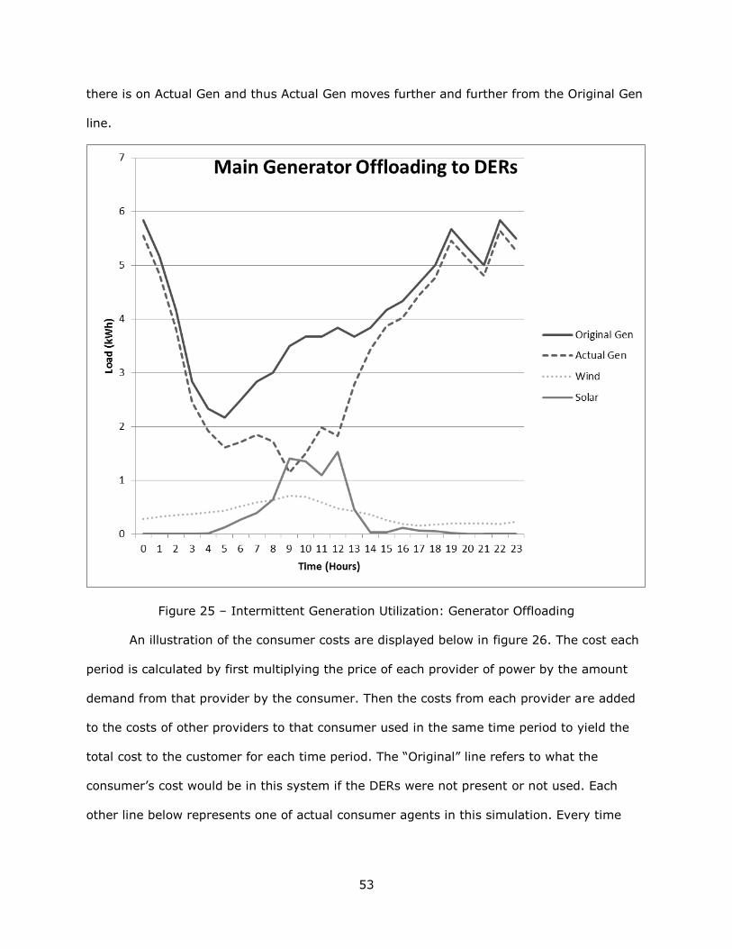
53
there is on Actual Gen and thus Actual Gen moves further and further from the Original Gen
line.
Figure 25 – Intermittent Generation Utilization: Generator Offloading
An illustration of the consumer costs are displayed below in figure 26. The cost each
period is calculated by first multiplying the price of each provider of power by the amount
demand from that provider by the consumer. Then the costs from each provider are added
to the costs of other providers to that consumer used in the same time period to yield the
total cost to the customer for each time period. The “Original” line refers to what the
consumer’s cost would be in this system if the DERs were not present or not used. Each
other line below represents one of actual consumer agents in this simulation. Every time

54
one of the consumer lines drops below the Original line it means that that consumer was
utilizing a DER to lower their costs.
Figure 26 – Intermittent Generation Utilization: Consumer Cost Reduction
Summarizing the costs from figure 26 above is table 4 below. The “Daily Cost”
column is simply the summation of the values used in figure 26 above. The “Weekly Cost”
column is the summation of the calculated cost data for the entire simulation run. Each of
the consumers saves approximately $4 a week over their standard rate by utilizing DER’s in
this simulation. This means that the system as a whole save nearly $12 in the week
simulated. Had this simulation incorporated a dynamic pricing mechanic the savings would
have been even greater as the lower load on the generator would likely have reduced its
price as well. It should be noted that because the generator is using a flat pricing function
(price is constant at base amount) the DERs are also simply charging their base prices. This
happens because in the uniform auction all of the consumer bids are at the exact same price
and thus in order to get under them and sell its entire stock a DER must charge their base
price. Later experiments will examine dynamic pricing and it related effect on DER prices
and utilization.

55
Table 4 – Intermittent Generation Utilization: Consumer Cost Reduction
Name Daily Cost Weekly Cost
Original (Without DERs) $4.92 $34.47
Con0 $4.57 $30.05
Con1 $4.40 $30.99
Con2 $4.55 $30.69
B. Consumer Demand Response
Consumer demand response is crucial to the positive impact of dynamic pricing as
well as for consumer cost minimization and as such it is important that consumers are able
to perform a demand response in such a way that saves them money, flattens the overall
load curve, while still protecting their privacy. In order to respond to long term bids,
generators need to have access to consumer demand information, however this information
is of a personal nature and many consumers may prefer to not have it shared with others.
To this end, the market design must not force consumers to share this information with
other consumers. With this concern in mind the demand response of consumer must still
allow them to save money. In order to determine if this is the case in the current design
simulation has been carried out at a variety of consumer demand response levels and
against a variety of pricing mechanisms. The below table contains the configuration data for
the agents tested in the following simulations. A 24 hour period was simulated. Each agent
was simulated individually alongside one of the generators. In total 12 simulations were
run.

56
Table 5 – Consumer Demand Response: Consumer Configuration
Name Demand Curve Shift-Ability
Zero Typical Summer Household 0%
One Typical Summer Household 1%
Five Typical Summer Household 5%
Ten Typical Summer Household 10%
Fifteen Typical Summer Household 15%
Twenty Typical Summer Household 20%
Table 6 – Consumer Demand Response: Generator Configuration
Name Capacity Base Price Price Function
QuadGen 2.7 kWh $0.15/kWh Quadratic RTP
OffPeakGen 2.7 kWh $0.15/kWh Off-Peak
In figure 27 below can be seen the price curves for both of the generator agents
described in table 6 above. These pricing functions have been discussed previously in the
Methods section and will be examined more closely in simulation in the next section. For
now they simply represent the price curves against which the agents will be responding to
with load shifting. These price curves have been generated by simply applying the typical
summer household demand curve (used by all of the agents above) as load to each of the
generators. The resulting price curves seen in the figure below represent the basic shape if
perhaps not the actuals prices that these pricing functions would produce in a real world
application. This is suitable for this test as demand response in this simulation acts based on
the relative prices over the course of a day rather than reacting to absolute price values.

57
Figure 27 – Consumer Demand Response: Pricing Functions
Figure 28 – Consumer Demand Response: Load Shifting Quadratic
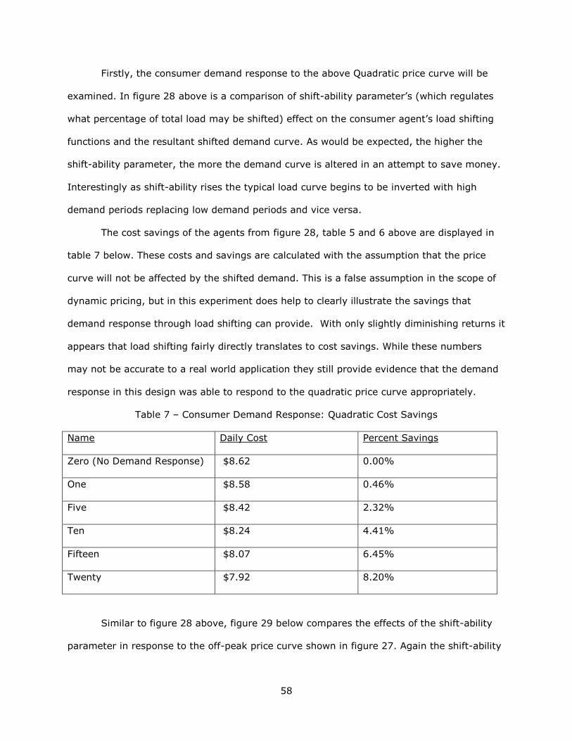
58
Firstly, the consumer demand response to the above Quadratic price curve will be
examined. In figure 28 above is a comparison of shift-ability parameter’s (which regulates
what percentage of total load may be shifted) effect on the consumer agent’s load shifting
functions and the resultant shifted demand curve. As would be expected, the higher the
shift-ability parameter, the more the demand curve is altered in an attempt to save money.
Interestingly as shift-ability rises the typical load curve begins to be inverted with high
demand periods replacing low demand periods and vice versa.
The cost savings of the agents from figure 28, table 5 and 6 above are displayed in
table 7 below. These costs and savings are calculated with the assumption that the price
curve will not be affected by the shifted demand. This is a false assumption in the scope of
dynamic pricing, but in this experiment does help to clearly illustrate the savings that
demand response through load shifting can provide. With only slightly diminishing returns it
appears that load shifting fairly directly translates to cost savings. While these numbers
may not be accurate to a real world application they still provide evidence that the demand
response in this design was able to respond to the quadratic price curve appropriately.
Table 7 – Consumer Demand Response: Quadratic Cost Savings
Name Daily Cost Percent Savings
Zero (No Demand Response) $8.62 0.00%
One $8.58 0.46%
Five $8.42 2.32%
Ten $8.24 4.41%
Fifteen $8.07 6.45%
Twenty $7.92 8.20%
Similar to figure 28 above, figure 29 below compares the effects of the shift-ability
parameter in response to the off-peak price curve shown in figure 27. Again the shift-ability

59
parameter performs as expected: The more shift-ability the more the demand curve is
altered to minimize costs. As should be apparent when comparing figure 28 and 29
however, is that the demand response is altered significantly by the price curve used. Unlike
the peak and valley of the quadratic price load shifting, off peak pricing promotes plateaus
of usage through the plateaus of price. The more a consumer is able to shift the more their
demand curve reflects these plateaus.
Figure 29 – Consumer Demand Response: Load Shifting Off Peak
Again like figure 28 and table 7 above, table 8 below summarizes the cost savings
from the demand curves presented in figure 29 above. Overall the total costs are less than
the quadratic price curve while the percent savings are up significantly. Rather than the
slightly diminishing returns of increasing shift-ability with quadratic real time pricing, with
off peak pricing there is actually an increasing return from higher levels of load shifting.
Though it should be noted once again that these results, like the ones in table 7, are based
on the assumption that the price curve will not adjust to the new demand amounts and as
such these numbers reflect more theoretical savings than realistic. None the less these

60
results do give evidence towards the effectiveness of consumer demand response in this
market design.
Table 8 – Consumer Demand Response: Off Peak Cost Savings
Name Daily Cost Percent Savings
Zero (No Demand Response) $7.96 0.00%
One $7.91 0.57%
Five $7.72 3.11%
Ten $7.48 6.42%
Fifteen $7.22 10.18%
Twenty $6.98 13.96%
C. Dynamic Pricing
The concept of dynamic pricing is crucial to the proposed Smart Grid for the benefits
it could provide. For this reason it is important that dynamic pricing is still a viable
mechanism in the negotiation and market design proposed in this paper. Specifically, the
two most prominent dynamic pricing functions, Off Peak, and Real Time Pricing, should be
performing as expected. To determine if this is the case, tests have been run in simulation.
Specifically, tests that investigate the consumer’s reaction and their associated savings as
well as the generator control and the flattening of their load curve. In table 9 below is
described the configuration parameters of the simulated agents for the first set of
experimental simulations on the quadratic dynamic pricing function. The simulation
contained 5 copies of the consumer described below as well as both of the generators.
Approximately a week’s worth of time was simulated.
Table 9 – Dynamic Pricing: Consumer Configuration
Name Curve Shift-Ability
Con(x5) Typical Household Summer 5%

61
Table 10 – Dynamic Pricing: Quadratic Generator Configuration
Name Capacity Base Price Price Function
ExpensiveGen 10 kWh $0.15 kWh Quadratic
CheapGen 10 kWh $0.10 kWh Quadratic
The price curves and load curves for a single day of the simulation are displayed in
figure 30 below. As their names, and the configuration data in table 10 above, would
suggest, ExpensiveGen has a higher base price than CheapGen and, as the data below
shows, is used less. The reason ExpensiveGen is used at all is because of the quadratic
pricing function. One of the functions of the dynamic pricing mechanic is to distribute load
so that no generator is loaded to capacity while another is nearly empty. It does this
through price incentives. As more consumers place their load on CheapGen its price rises in
accordance to the quadratic pricing function. As the price for CheapGen rises ExpensiveGen
begins to look more and more appealing to consumers until eventually CheapGen’s price is
driven above ExpensiveGen and consumer begin to make contracts with ExpensiveGen. The
curves below show this small simulated system’s load distribution equilibrium. In a larger
system with more consumers the gap between the two generator’s price curves would be
much smaller as each consumer’s load would affect the generator’s price less dramatically.
Figure 30 – Dynamic Pricing: Quadratic Generator Loads and Prices
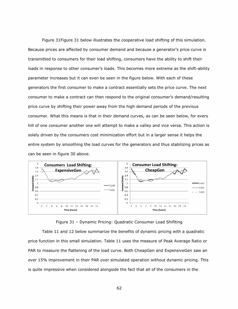
62
Figure 31Figure 31 below illustrates the cooperative load shifting of this simulation.
Because prices are affected by consumer demand and because a generator’s price curve is
transmitted to consumers for their load shifting, consumers have the ability to shift their
loads in response to other consumer’s loads. This becomes more extreme as the shift-ability
parameter increases but it can even be seen in the figure below. With each of these
generators the first consumer to make a contract essentially sets the price curve. The next
consumer to make a contract can then respond to the original consumer’s demand/resulting
price curve by shifting their power away from the high demand periods of the previous
consumer. What this means is that in their demand curves, as can be seen below, for every
hill of one consumer another one will attempt to make a valley and vice versa. This action is
solely driven by the consumers cost minimization effort but in a larger sense it helps the
entire system by smoothing the load curves for the generators and thus stabilizing prices as
can be seen in figure 30 above.
Figure 31 – Dynamic Pricing: Quadratic Consumer Load Shifiting
Table 11 and 12 below summarize the benefits of dynamic pricing with a quadratic
price function in this small simulation. Table 11 uses the measure of Peak Average Ratio or
PAR to measure the flattening of the load curve. Both CheapGen and ExpensiveGen saw an
over 15% improvement in their PAR over simulated operation without dynamic pricing. This
is quite impressive when considered alongside the fact that all of the consumers in the

63
system were only willing to shift 5% of their total load. This reduction in PAR allows
generators to operate in a smaller outputs range as they don’t have to meet as high of
highs or as low of lows in their load. This allows then to run more efficiently and thus
ultimately save their operators money. Table 12 below summarizes the costs to each
consumers attached to their respective generator. The “Costs Old” column refers to the
simulated results of the agents without load shifting whereas the “Costs New” column refers
to the results of the simulation discussed above. Here again benefits are seen in the form of
reduced costs to consumers. It should be noted that the results of table 12 differ from those
in table 8 in that the consumer response is being reincorporated back into the price curve
due to the use of a quadratic real time dynamic price mechanism by the generators. Both
table 11 and 12 give evidence to the positive effects of quadratic dynamic pricing and its
implementation in this market and simulation.
Table 11 – Dynamic Pricing: Quadtatric PAR reduction
Name PAR Old PAR New % Reduction
CheapGen 1.42 1.19 16.54%
ExpensiveGen 1.42 1.20 15.43%
Table 12 – Dynamic Pricing: Quadratic Cost Savings
Name Cost Old
($/Day/Person)
Cost New
($/Day/Person)
% Reduction
CheapGen 6.56 6.28 4.53%
ExpensiveGen 7.31 7.10 2.77%
With quadratic pricing now simulated, and examined, it comes time to determine the
effects of an off-peak dynamic pricing mechanism in this market model. In table 13 and
table 14 below are the configuration parameters for the agents of this off-peak pricing
experimental simulation environment. The consumer agents are identical to those used in

64
the quadratic dynamic pricing simulation above. The generators use the Off-Peak pricing
model rather than quadratic real time pricing in this simulation. They have also had their
capacity reduced. This is because the effectiveness of Off-Peak pricing depends on
generator load fluctuating between on and off peak load amounts. Because, in this
simulation’s implementation, the threshold between on and off peak is set at half of the
total capacity it is important that the capacity be roughly twice the average hourly demand
so that the off-peak price changes come into play.
Table 13 – Dynamic Pricing: Off Peak Consumer Configuration
Name Curve Shift-Ability
Con(x5) Typical Household Summer 5%
Table 14 – Dynamic Pricing: Off Peak Generator Configuration
Name Capacity Base Price Price Function
ExpensiveGen 8.2 kWh $0.15/kWh Off-Peak
CheapGen 8.2 kWh $0.10/kWh Off-Peak
Figure 32 below shows the load and price curves for ExpensiveGen and CheapGen
from the simulation described above. Similar to figure 30Figure 30 for quadratic pricing, the
figure below illustrates how equilibrium is reach between the two generators. Unlike in
quadratic however, prices are not as responsive to loads and so the two price curves will
remain further apart no matter the size of the simulation. Regardless, the distribution of
load between generators is still effective.

65
Figure 32 – Dynamic Pricing:Off Peak Generator Loads and Prices
In figure 33Figure 33 below are shown the shifted demand curves for the consumers
contracted with ExpensiveGen and CheapGen respectively. As is obvious from these curves,
all of the consumers shifted their demand in the exact same way. This is because of the Off-
Peak pricing mechanism. Since prices do not actually reflect load in a direct way consumers
are unable to respond to other consumer demand curves through the transmission of
generator prices. So instead of responding to an actual price curve consumers instead
simply try to demand curve flatten in an effort to avoid peak prices and since all of the
consumers in this experiment have the same typical demand curve they all flatten in the
same way.
Figure 33 – Dynamic Pricing: Off Peak Consumer Load Shifting
The summary of the benefits from the above simulation can be found in table 15 and
16 below. From the generator’s perspective Off-Peak performs very similarly to quadratic
with an approximately 15 percent reduction in Peak Average Ratio. Unfortunately the story

66
is not so good for consumers, who only saved between 3 and 0 percent through their load
shifting. On the other hand however consumers did pay less overall. These results still point
to the effectiveness of Off-Peak pricing in the system even if it is lessened in comparison to
Quadratic pricing.
Table 15 – Dynamic Pricing: Off Peak PAR Reduction
Name PAR Old PAR New Percent Reduction
CheapGen 1.42 1.20 15.43%
ExpensiveGen 1.42 1.20 15.43%
Table 16 – Dynamic Pricing: Off Peak Cost Savings
Name Cost Old
($/Day/Person)
Cost New
($/Day/Person)
Percent Reduction
CheapGen 5.41 5.24 3.11%
ExpensiveGen 4.92 4.92 0.00%
D. Integration
In order to be an effective negotiation and market design it must be able to integrate
all of the parts described above and still perform effectively. Effective performance is in this
case is defined as the assignment of resources such that costs across the system are
minimized. While true optimality would obviously be preferred it is difficult to achieve
without explicitly prescribing the actions of every participant which is nearly the precise
opposite of an open and distributed market structure. It is hoped that in small scale
simulations the market will be able to integrate all of its disparate parts and operate
effectively. It is then hoped that as simulations scale upwards that the results remain
consistent and thus hopefully continue to be effective. Ultimately, being an effective market
will require consumers getting the lowest possible cost, low cost DERs being fully used, and
generators being utilized in a balanced manner as determined by their prices. In order to

67
determine if this is the case a small scale simulation has been executed with the below
agent parameters as defined in Table 17, 18 and 19.
Table 17 – Integration: Consumer Configuration
Name Demand Curve Shift-Ability
Con(x5) Typical Household Summer 5%
Table 18 – Integration: Generator Configuration
Name Capacity Base Price Price Function
ExpensiveGen 10 kWh $0.10/kWh Quadratic
CheapGen 10 kWh $0.10/kWh Quadratic
Table 19 – Integration: DER Configuration
Name Capacity Curve Base Price
SolarDer Small Solar $0.05/kWh
WindDer Small Wind $0.10/kWh
Figure 34Figure 34 below displays the generator price curves from a day of this
simulation. Because of the quadratic price function and the relatively low number of the
consumers the price curve is quite unstable and yet even so it is easy to see that the
system has reached equilibrium just like in the dynamic pricing experimental simulations
presented in figure 30Figure 30. Both of the generators have fairly equal prices, and in fact
they switch places momentarily throughout the day.

68
Figure 34 – Integration: Generator Prices
The associated loads from the above generators and prices are shown in figure
35Figure 35 below. Obviously the integration of DERs into a system with quadratic dynamic
real time pricing functions causes some instability in loads and therefore and prices. It is no
accident however that ExpensiveGen’s and CheapGen’s are closer in this simulation than in
the previous one. As can be seen below the DERs have helped to equalize the system even
further by favoring the more expensive ExpensiveGen’s consumers and thus lowering its
load and prices. The alternating valleys of the actual loads are caused by the crossovers of
price as seen in figure 34Figure 34 above. As described in the secondary market design,
DER’s select consumers based on their bid prices which are related to the prices they are
currently paying to their primary market generator. So when the primary market
generator’s prices cross over each other so too does the preference of secondary market
DERs.

69
Figure 35 – Integration: Generator Loads
Figure 36 – Integration: Expensive Gen Consumer Demands

70
To further expand the generator loads, figure 36 above shows the associated
consumer demand curves of generator CheapGen. The blunting of the demand curves as
well as the reactions against other consumer demands are easily seen below. The large
drops in demand are of course due to the consumers offloading their demand to cheaper
DERs that period.
Figure 37 – Integration: CheapGen Consumer Demands
Again expanding on a generator load is figure 37Figure 36 above illustrating the consumer
demands associated with the generator ExpensiveGen. Due to its higher prices, the
consumers of ExpensiveGen have seen far more DER usage and it reflects in their
apparently unstable load curves. Given two equal bids a DER will randomly select among
them and as such tends to evenly distribute its power among evenly bidding consumers
such at the two below attached to the same generator. This is the cause of the seemingly
wild fluctuations in demand on the parts of Con1 and Con2.

71
Figure 38 - Integration: WindDer Load
Figure 39 – Integration: SolarDer Load

72
To find the cause of all of this offloading the DER loads and their usage must be
examined. Above is figure 38 which displays the load of WindDER and its constituent
consumer demands. Again here is seen the preference given to Con1 and Con2 due to their
more expensive primary generation. The fair distribution of usage between the two agents
is also once again seen below. It should be noted that while Con1 and Con2 are
overwhelming preferred Con4 does slip in during one of the few price crossovers as seen in
figure 34Figure 34.
Similar to figure 38, figure 39 above shows the load and usage of SolarDer. Again
the ExpensiveGen consumers dominate, but due to SolarDer’s high overall capacity more
agents get a piece of it. It should be noted that in both the figure below and the one above
that the DERs are being used to capacity similar to the original simulations of them in figure
24.
The tables below summarize the results of this small scale integration simulation
test. The results for the most part follow the expectations set by previous simulations. Table
20 on the other hand does present a problem with the worsening of PAR for ExpensiveGen.
This can be explained by ExpensiveGen’s high usages of DERs which while lowering its peak
also dramatically lowered its average load. As can be seen through the results of CheapGen
the dynamic pricing system for reducing PAR is still effective it appears however that high
prices will encourage offloading demand to DERs which will in turn destabilize a generator’s
load curve and thus raise PAR.
Table 20 – Integration: PAR Reduction
Name PAR Old PAR New Percent Reduction
CheapGen 1.42 1.26 11.43%
ExpensiveGen 1.42 1.47 -3.39%

73
Table 21 – Integration: PAR Reduction
Name Costs Old
($/Consumer/Day)
Costs New
($/Consumer/Day)
Percent Reduction
CheapGen $6.56 $6.25 4.74%
ExpensiveGen $7.31 $6.97 4.56%
E. Scalability
Because proposed and existing Smart Grid technologies tend to be based on low
power embedded computing devices it is important that any locally run software agent be
low enough in complexity to operate on these types of devices effectively. Because the
Smart Grid will be large in size is it is also important that the negotiations can scale
effectively. The simulation can help examine both of these concerns in the design. Below in
table 22 is the breakdown of the complexity and scalability simulation setup. Table 23
contains some basic specifications on the computer running the simulation. The simulation
will be executed with varying numbers of agents and the execution time will be examined to
determine how the negotiation performance scales.
Table 22 – Scalability: Agent Configuration
Percentage of Total Agent Type
60% Consumer
10% Generator
30% DER (Wind)
Table 23 – Scalability: Computer Specification
Processor Speed 2.8 GHz
Processor Cores 6
System Memory 8 GB

74
The execution time results of the three simulations are contained in table 24 below.
Figure 40Figure 40 below illustrates the exponential nature of the execution time growth.
What these results display is that as the number of agents in the system grows so too does
the complexity of each agent’s execution. Not only does it take longer to simulate a 24 hour
period the more agents there are but it also takes longer to simulate each agent. This is
because the more agents there are the more communication and analysis each agent must
perform in order to negotiate for a contract. While these results may be simply due to
inefficiencies in the simulation itself, it seems likely that this exponential growth in
complexity as the number of participants grows is an inherent consequence of the market
design.
Table 24 – Scalability: Execution Time
Number of Agents Time to simulate a 24 hour period Time/Agent/Day
25 5.9 seconds 0.2 seconds
50 19.2 seconds 0.4 seconds
75 47.1 seconds 0.6 seconds
100 1 minute 31 seconds 0.9 seconds
125 2 minutes 48 seconds 1.3 seconds
150 5 minutes 29 seconds 2.3 seconds
Figure 40 – Scalability: Execution Time

75
IV. DISCUSSION & CONCLUSION
A. Discussion of Results
In order to evaluate the proposed power market design five aspects of the design
were tested in simulation. Does the design fully utilize intermittent energy resources? Does
the design allow for consumer demand response through load shifting? Does the design
facilitate and promote the real time dynamic pricing of power? Do all of the aspects of the
market work together to produce effective resource allocation? Does the design scale
upwards while still remaining effective?
DER utilization was one of the key aspects of the market design and was the driving
force behind the decision to implement a 2 market structure. The results from section A of
the Results section above do indeed indicate that DER resources are being utilized fully and
that their usage is reducing costs for consumers. Table 4 and figure 24 in particular display
the off-loading of demand from primary market generation to DERs and the savings
incurred for consumers by doing so. Ultimately it was determined through simulation
modeling and testing that intermittent energy resources could be integrated into the system
and utilized as best able to reduce load on main generators and save consumers money.
Consumer demand response can be extremely beneficial both for the consumers
themselves and for the health of the grid overall and thus it was extremely important that it
operate effectively in the proposed market design. The results presented in section B of the
Results chapter indicate that this is indeed the case. Both a quadratic real time and off-peak
pricing function were used to evaluate the demand response of customers as well as
compare a range of shift-ability values. Figure 28Figure 28 and table 7 of that section
illustrate the effectiveness of consumer demand response to a quadratic dynamic pricing
function with consumers saving a significant amount of money across the board. Figure 28
and table 8 illustrate the effectiveness of consumer demand response to an off-peak
dynamic pricing function. Consumers, in fact, saved even more money in response to off-
peak pricing than they did in response to quadratic. These results would be tempered by the

76
later dynamic pricing testing results. Overall however these results generated through
simulation modeling and testing have indicated that Consumer Demand Response is still a
viable way for consumers to save money.
The dynamic pricing of electricity is used to promote consumer demand response
and as such plays a vital role in the potential gains of the smart grid and of this proposed
market design. Section C of the Results chapter above details the tests done on this aspect
of the market design and simulation. Once again the two most common dynamic pricing
functions were tested: quadratic real time and off-peak. Figure 30Figure 30 and 31Figure 31
along with table 11 and 12 display the results of the quadratic pricing function testing.
These results show that quadratic pricing was able to effectively balance usage and prices
between generators as well as lower the PAR and still save consumer’s money. The
quadratic results also display how cooperative load shifting takes place without direct
communication between consumers. Figure 32 and 33 along with table 13 and 14 illustrate
the results of the off-peak pricing function tests. These results indicate that while off-peak
pricing does lower the PAR further than quadratic, it does not incentive nor facilitate
demand response through load shifting as well as quadratic real time pricing does. In the
end these results show that Dynamic Pricing is still a viable and effective method of
regulating power usage through not all forms of dynamic pricing are as viable and effective
as others.
Ultimately all of the above aspects of the design would be worthless if they could not
operate alongside and in cooperation with one another to produce effective resource
allocation results. That is why in section D of the Results chapter above testing was
performed on the fully integrated market and the results presented. Table 21 and 22
summarize the results of this section and show that the dual markets and various aspects
do integrate successfully and allow consumers to save a significant amount of money. On
the other hand however the results indicate that the integration of the DER market acts to
destabilize the load on generators and can actually increase PAR in certain situations.

77
Overall the results indicated that the various aspects the market can be integrated together
and that needs of all participants can be met in an effective fashion if perhaps some more
than others.
The final aspect of the design to be modeled simulated and tested was the scalability
of the market along with an individual agent’s ability to run on low power hardware. The
electrical grid is a massive interconnected system and as such any market model must be
able to scale upwards and involve large numbers of participants while still keeping each
individual participant low enough in complexity to run on smart meters and the like. The
results of this testing are report in section E of the Results chapter. Figure 40 effectively
summarizes the results of these tests. It was found that the time to simulate a 24 hour
period increased exponentially as the number of participants rose. This indicates that in the
proposed market design the complexity of operating an individual agent increases
exponentially as the number of agents in the market rises. While this was not unexpected it
does raise doubts as to the effective scalability of this market design as well as an individual
agent’s ability to operate on low power hardware.
B. Validation
In order to keeps the results of the simulation reflective of real world power usage all
of the usage and generation data have been sourced from real world readings. Typical
consumer household load data was taken from [58]. DER capacity curves for wind and solar
were taken from [56] and [57] respectively. By using actual load and generation data it is
hoped that the general shapes and thus behavior of consumers and DERs can be modeled.
It was not the intention of the modeling to create a perfectly accurate period by period
representation of their costs and so forth.
The results above are presented, not as the precise or accurate measures of the
effects on the market participants, but as indicators of the general actions of this market
design in an effort to determine if the proposed design is at all valid or effective. Because of

78
this the results data itself would likely not be valid as representing a real world
implementation. That is to say, for instance, consumers may not save 4% on their
electricity bills and generators may not reduce their PAR by 11% but in general then can
still be used to help determine whether or not the design allows consumers to save money
at all or whether it allows generators to reduce their PAR at all. In this way the results are
valid for their intended purpose.
C. Advantages and Limitations
In comparison to the existing electrical grid system as well as in comparison to other
research work the proposed market design has a number of advantages as well as a
number of limitations. The automated and distributed nature of the market sets this design
apart from many comparable research works as well as from the current electrical grid. The
three participant types defined in the market are unique to this design. Finally the 2 market
structure is novel both in comparison to existing research and to the current grid.
That this market design is distributed and autonomous through its use of agents is
fairly rare though not entirely unique among existing research, as discussed in the literature
review. The autonomous nature of the design has the advantage of allowing complex
participant interactions and behaviors without significant time and energy investment from
the actual participant. The lack of central control facilitated by the distributed nature of the
design allows the system to be extremely flexible with individual participants entering and
exiting the system without any severe impact on the system as a whole. This distribution of
control does come at a price however as shown in the scalability tests discussed above.
Communications overhead rises dramatically as the system increases in size and agents
must all individually communicate with each to negotiate contracts. This high
communications overhead also means that communications infrastructure must be robust in
order to facilitate it and the participant agent hardware itself must be powerful in order
operate on it. This scalability limitation means that this market design would most likely be

79
best suited for use within fairly small microgrid or amongst collective negotiators, such as a
neighborhood acting as a single consumer.
The three participant structure of the market is a novel part of the proposed design.
These three categories of participants allow the complex nature of the grid to be unified into
3 simple categories while still retaining and catering to their unique and fundamental
differences. Consumers of all types can be represented by a single type of consumer agent
and simply customize it’s parameters to better represent their unique needs. This allows
them to participate and receive the benefits of the negotiation market without themselves
needing to be particularly invested. Reliable generation sources of all types can be
represented by a generator agent and participate in the market. By doing so, they can
flatten their load curve and thus lower their PAR (for the most part) by a significant degree.
Unfortunately for reliable generator participants the involvement of DERs appears to
destabilize their load curves and thus, in some cases, negate the smoothing impact of
dynamic pricing. DERs of all types can be participants in the market through representation
by a DER agent. Through the use of this agent they can fully sell their generated power
whenever it is available thus encouraging the use of cheap, often renewable, energy,
resources. These participants are limited by the assumptions that must be made about
them in order for them to enter the market however. All participants must be equipped with
the hardware necessary to run their representative agent as well as communicate with the
rest of the market. Consumers in particular must be equipped with the required technology
to both monitor and control the energy demand of the participant (Smart Meter and ECC).
Central to the design is the two market structure proposed. This structure has the
advantage of catering to the needs of each type of participant. Consumers wish to have
reliable power delivered to them while still being able to respond to changes in price.
Generators wish to control their load so as to avoid expensive peak generation. Thus the
primary market allows them to do so. DER participants wish to sell all of their capacity
whenever it is available while consumers which to save money by using cheaper generation

80
sources when they are available. Thus the secondary market allows them to do so.
Ultimately this two market structure allows consumers to have the reliability of primary
generation sources while still being able to save money through the use of low cost
intermittent energy resources. A limitation of this two market structure is the fact that
extra-normal participant behavior in an attempt to “game” the market has not been
considered. It may be possible for participants to gain an advantage for themselves by
acting in ways not prescribed by the market design. Generator collusion for example could
effectively raise prices dramatically for the entire market. Likely the largest limitation of this
two market negotiation structure is that it does not result in optimal solutions. While
preferable solutions are incentivized by the market design the very nature of the distributed
market based negotiation means that it is very difficult to ensure optimality.
D. Implications
In a larger sense, this proposed market design, modeling, simulation, and testing
has a number of implications. It has added to the evidence that distributed and autonomous
electrical power contract negotiation is viable. It has shown that a purely market driven
design is viable for electrical grid resource allocation. It has shown that DERs can be
successfully integrated and should be considered separate from regular generation to do so.
It has shown how cooperative consumer demand response can operate without direct
consumer to consumer communication. It has shown some of the issues related to off-peak
pricing.
While certainly not completely novel among the existing research, distributed and
autonomous negotiating resource allocation in the electrical grid is a fairly new and little
researched topic. The design and results presented here should help to further encourage
research into this area as a viable alternative to centralized control techniques. The
communications overhead to this design is perhaps prohibitive but in comparison to
centralized control it may actual offer improved scalability.

81
Of the reviewed research the proposed entirely market based electrical grid resource
allocation design appears to be completely new. It is hoped that the viability of this
technique will be further considered as an alternative to standard optimization methods. By
incentivizing globally optimal agent behavior rather than simply proscribing it, all
participants are able to simply act in their own self-interest and ultimately come to, while
not an optimal solution, an effective one.
The in the proposed market design the method of encouraging DER usage appears to
be novel among the reviewed research. DERs such as wind and solar energy tend to have
significantly unstable generation capacities over time. Because of this, it this is useful to
treat them differently from normal sources of electricity generation. Hopefully the positive
results of this design and the specific negotiation market to facilitate DER usage will push
others to consider the issue as well. DERs likely present the most viable option for effective
renewable energy production and any market incentive towards their use should be strongly
considered.
The method of cooperative demand response among consumers as used in the
proposed design is novel among the reviewed research. Instead of having consumers
directly contact each other in order to cooperatively schedule power usage (as has been
proposed in other research) consumers use the price curve as well as their own demand
curve to shift power and through the generator communicate their curves to one another.
As the results show, this keeps consumers from syncing their shifted power during the low
price periods while still allowing each consumer to keep their demand curve relatively
private.
Off-Peak pricing is one of the more popular dynamic pricing mechanisms but this
research seems to indicate it’s generally less effective nature when compared to a quadratic
real time pricing mechanism when used in combination with autonomous demand response.
The primary advantage of off-peak pricing is in its simplicity but in the proposed market
design that simplicity worked against it. Off-peak pricing did not as greatly incentivize

82
consumer demand response and also did not facilitate cooperative load shifting. Hopefully
these results will encourage researcher to reevaluate the usefulness of off-peak pricing in
autonomous demand response systems such as in the proposed design.
E. Feasibility
An important question pertaining to the proposed market design is the feasibility of
said design. Current technological trends indicate that this design would likely be infeasible
for large scale implementation in the 5-10 years. It would require that every consumer be
equipped with fully automated smart homes capable of controlling the internal electrical
devices as well as communicating with other market participants. This technology is
theoretically available to consumers today but the nearly uniform use of it assumed by this
design will likely not occur in the near future. Along with that the robust communications
infrastructure required to enable nearly continuous communications amongst all of the
participants of the system simultaneously has not yet been established. When this fact is
combined with the results of the scalability testing, which show that the communications
overhead grows exponentially as the number of participants increases, means that the work
to build the needed infrastructure would likely be prohibitively expensive in the near term.
Likely most prohibitive to the system’s feasibility however is the fact that a large majority of
electrical grid “middle men” would be removed or their roles dramatically changed by the
proposed design. Such changes would require radical alterations to federal and local energy
policies and structuring which rarely happen quickly.
Small scale implementations are far more feasible. Within a single small town or
even neighborhood all participants could be equipped with the proper devices and
communications infrastructure. Large scale implications with a low granularity are also more
feasible, with entire groups of physical participants being represented by a single agent.
Regardless, even then, further testing and refinement of the design itself would be required
to prepare it for real world use.

83
Overall the proposed design was not intended for real world use. Its purpose is as an
examination of possibilities. It is hoped that some of the principles and ideas from it might
help to promote further investigation into alternative electrical grid designs or even help
improve existing systems. In this way it is not necessarily important that the market be
feasible but that it be viable and effective in interesting ways which, as the results above
show, it seems to be.
F. Future Research
In developing the simulator for the purposes of evaluating the proposed market the
application was created to be highly flexible and configurable. This allows for a large amount
of future research to be conducted on the existing simulator or through the extension of the
existing simulator. Due to the wide breadth of this paper there remains a prodigious amount
of research problems yet to be investigated.
As noted previously there are scalability issues with the proposed design. This is not
an uncommon problem for distributed systems and there may be many possible solutions to
this problem that might be investigated and evaluated. Only two dynamic pricing functions
were examined in the course of this research and even then only a brief investigation into
each of them was conducted. Many more dynamic pricing functions exist and even the two
previously discussed likely deserve further examination. Along with dynamic pricing the
consumer response to it also provides a number of available research questions. What
might be the effects of a variety of shift-ability consumers existing within the same
environment? What might some alternative load shifting algorithms be and how might they
perform better? Sorely lacking in the market implementation above is a fully realized price
prediction algorithm. Effective price prediction might dramatically improve the ability of
consumers to effectively select generators and engage in demand response. The testing
conducted on the market design solely involved household consumers and their typical load
profiles. Other types of consumers might behave quite differently and should be

84
investigated. Likely the largest research problem left unanswered by the current design,
modeling, simulation, and testing is that of actual electricity transmission and distribution.
The simulator would likely need significant extension in order to accommodate these
consideration but they are critically important parts of the electrical grid and a resource
allocation market of any kind would likely benefit from taking them into account.
G. Conclusion
In order to answer the question of how can power be bought and sold in such a way
that the difficulties of centralized control, integration of unstable DERs, the dynamic pricing
of power and the privacy, demand response, and low computational ability of customers is
all taken into account, a new distributed autonomous negotiation based power market was
proposed. The proposed design incorporates a distributed and autonomous agent based
contract negotiation system in which participants, represented by the agents, engage in two
distinct yet interconnected markets in order to determine resource allocation. The primary
market is organized as a sealed bid first price reverse auction and deals in day long
contracts from generators able to guarantee reliable power generation over that period. The
secondary market is organized as a uniform price auction and deal in hour long contracts
from intermittent energy resources that generate power inconsistently and wish to be used
opportunistically. Agents representing reliable generation are responsible for forecasting
future prices and loads as well as providing that information to buyers. Consumer agents in
the primary market select their generators based upon the prices and load schedules
provided to them in an attempt to minimize the cost to meet their demand. Agents
representing intermittent energy resources attempt to sell all of their available electrical
generation whenever possible. Consumer agents in the secondary market attempt to use
intermittent energy resources to meet power demand in yet another attempt to minimize
costs. After contract negotiation consumers further attempt to minimize their costs by
shifting a certain percentage of their load from high cost to low cost periods.

85
In order to evaluate the above design a simulation was developed and the proposed
market design was modeled and tested within it. A set of specific aspects of the design were
chosen to determine its effectiveness. The first aspect tested was intermittent energy
resource integration and utilization in the system as best able to reduce load on main
generators and save consumers money. The next aspect tested was consumer demand
response as an effective and a viable way for consumers to save money. In conjunction with
consumer demand response dynamic pricing was tested to determine if it was a viable and
effective method of regulating power usage while still allowing consumers to save money.
These aspects were then put together to test the integration of all of the disparate systems
and to determine if the needs of all participants can be met effectively. Finally testing was
conducted to determine if the representative agents have low enough computational
requirements as to be able to run on integrated computers such as smart meters while still
being able to scale upwards to the large sizes required by the electrical grid.
The results of the above testing have shown that the proposed design is a viable and
at least somewhat effective method of allocating electrical grid resources amongst
consumers, generators, and intermittent energy resources. Intermittent energy resources
are fully utilized within the system and do act to save consumer’s money. Consumer
demand response is an effective method of saving money for consumers and when utilized
by primary generation does allow generators to control load through load balancing and the
smoothing of the load curve. When put together these systems do still operate effectively
though the instability of the secondary DER market does negatively affect the load curves of
the primary generation market. The proposed design does have scalability issues with the
system and agent complexity increasing exponentially as the number of participants
increase. Even so, the proposed design has withstood initial investigation and appears to be
a viable and even effective, if perhaps not highly feasible, approach to resource allocation
for a smart electrical grid.

86
VI. REFERENCES
[1] J. Wellinghoff, "Prepared Testimony of Jon Wellinghoff, Commissioner Federal Energy
Regulatory Commission Before the House Energy and Commerce Subcommittee on
Energy and Air Quality," Federal Energy Regulatory Commission, 2007.
[2] J. Osborn and C. Kawann, "Reliability of the U.S. Electricity System: Recent Trends and
Current Issues," Energy Analysis Department Enviromental Energy Technologies
Division, Berkeley, 2001.
[3] Litos Strategic Communication, "The Smart Grid: An Introduction," U.S. Department of
Energy, 2008.
[4] L. Kannberg, D. Chassin, J. DeSteese, S. Hauser, M. Kinter-Meyer, R. Pratt, L.
Schienbein and W. Warwick, "GridWiseTM: The Benefits of a Transformed Energy
System," United States Department of Energy, 2003.
[5] A. P. S. Meliopoulos, G. Cokkinides, R. Huang, E. Faratatos, S. Choi, Y. Lee and X. Yu,
"Smart Grid Technolgies for Autonomous Operation and Control," IEEE Transactions on
Smart Grid, vol. 2, no. 1, pp. 1-10, 2011.
[6] A. A. Aquino-Lugo, R. Klump and T. J. Overbye, "A Control Framework for the Smart
Grid for Voltage Support Using Agent-Based Technologies," IEEE Transactions on Smart
Grid, vol. 2, no. 1, pp. 173-180, 2011.
[7] R. Podmore and M. R. Robinson, "The Role of Simulators for Smart Grid Devleopment,"
IEEE Transactions on Smart Grid, vol. 1, no. 2, pp. 205-212, 2010.
[8] W. Ketter, J. Collins and C. Block, "Smart Grid Economics: Policy Guidance through
Competitive Simulation," Eramus Research Institute of Management, Rotterdam, 2010.
[9] M. A. Ortega-Vazquez and D. S. Kirschen, "Assessing the Impact of Wind Power
Generation on Operating Costs," IEEE Transactions on Smart Grid, vol. 1, no. 3, pp.

87
295-301, 2010.
[10] S.-Y. Su, C.-N. Lu, R.-F. Chang and G. Gutierrez-Alcaraz, "Distributed Gneration
Interconnection Planning: A Wind Power Case Study," IEEE Transactions on Smart
Grid, vol. 2, no. 1, pp. 181-189, 2011.
[11] F. Rahimi and A. Ipakchi, "Demand Response as a Market Resource Under the Smart
Grid Paradigm," IEEE Transactions on the Smart Grid, vol. 1, no. 1, pp. 82-88, 2010.
[12] P. Nyeng and J. Ostergaard, "Information and Communications Systems for Control-by-
Price of Distributed Energy Resources and Flexible Demand," IEEE Transactions on
Smart Grid , vol. 2, no. 2, pp. 334-341, 2011.
[13] A. Faruqi, R. Hledik and J. Tsoukalis, "The Power of Dynamic Pricing," The Electricity
Journal, vol. 22, no. 3, pp. 42-56, 2009.
[14] M. M. R. Khan, "Modeling of Consumer Responses to Dynamic Pricing in a Smart Grid,"
North Dakota State University, Fargo, 2012.
[15] A. Faruqui and S. Sergici, "Household Response to Dynamic Pricing of Electricity -- A
Survey of the Experimental Evidence," Brattle Group, 2009.
[16] H. Saele and O. S. Grande, "Demand Response From Household Customers:
Experiences From a Pilot Study in Norway," IEEE Transaction on Smart Grid, vol. 2, no.
1, pp. 102-109, 2011.
[17] M. Roozbehani, M. Dahleh and S. Mitter, "Dynamic Pricing and Stabilization of Supply
and Demand in Modern Electric Power Grids," in IEEE International Conference on
Smart Grid Communications, 2010.
[18] H. Allcott, "Rethinking Real Time Electricty Pricing," Center for Energy and
Enviromental Policy Research, 2009.
[19] H.-p. Chao, "Price-Responsive Demand Management for a Smart Grid World," The
Electricity Journal, vol. 24, no. 1, pp. 7-20, 2010.

88
[20] S. K. Aggarwal, L. M. Saini and A. Kumar, "Electricity price forecasting in deregulated
markets: a review and evaluation," Electrical Power and Energy Systems, vol. 31, pp.
13-22, 2009.
[21] N. Amjady, F. Keynia and H. Zareipour, "Short-Term Load Forecast of Microgrids by a
new Bilevel Prediction Strategy," IEEE Transactions on the Smart Grid, vol. 1, no. 3,
pp. 286-294, 2010.
[22] S. Shakiba, M. Piltan, S. F. Ghaderi and M. S. Amalnik, "Short-term Electricity
Forecasting in Deregulated Markets using Artificial Neural Networks," in Proceedings of
the 2011 International Conference on Industrial Engineering and Operations
Management, Kuala Lumpur, 2011.
[23] P. Du and N. Lu, "Appliance Commitment for Household Load Scheduling," IEEE
Transactions on Smart Grid, vol. 2, no. 2, pp. 411-419, 2011.
[24] A. Kamilaris and A. Pitsillides, "Exploiting Demand Response in Web-based Energy-
aware Smart Homes," in The First International Conference on Smart Grids, Green
Communications and IT Energy-aware Technologies, Venice, 2011.
[25] T. Jin and M. Mechehoul, "Ordering Electricity via Internet and its Potentials for Smart
Grid Systems," IEEE Transactions on Smart Grid, vol. 1, no. 3, pp. 302-310, 2010.
[26] A.-H. Mohsenian-Rad and A. Leon-Garcia, "Optimal Residential Load Control With Price
Prediction in Real-Time Electricity Pricing Enviromnments," IEEE Transactions on Smart
Grid, vol. 1, no. 2, pp. 120-133, 2010.
[27] T. T. Kim and H. V. Poor, "Scheduling Power Consumption with Price Uncertainty," IEEE
Transactions on Smart Grid, vol. 2, no. 3, pp. 519-527, 2011.
[28] A.-H. Mohsenian-Rad, V. W. Wong, J. Jatskevich, R. Schober and A. Leon-Garcia,
"Autonomous Demand-Side Management Based on Game-Theorectic Energy
Consumption Scheduling for the Future Smart Grid," IEEE Transaction on Smart Grid,

89
vol. 1, no. 3, pp. 320-331, 2010.
[29] S. Hatami and M. Pedram, "Minimizing the Electricity Bill of Cooperative Users under a
Quasi-Dynamic Pricing Model," in First IEEE International Conference on Smart Grid
Communications, 2010.
[30] A. J. Conejo, J. M. Morales and L. Baringo, "Real-Time Demand Response Model," IEEE
Transactions on Smart Grid, vol. 1, no. 3, pp. 236-242, 2010.
[31] P. Samadi, A.-H. Mohsenian-Rad, R. Schober, V. W. Wong and J. Jatskevich, "Optimal
Real-Time Pricing Algorithm Based on Utility Maximization for Smart Grid," in First IEEE
International Conference on Smart Grid Communications, Vancouver, 2010.
[32] R. G. Smith, "The Contract Net Protocol: High-Level Communication and Control in a
Distributed Problem Solver," IEEE Transactions on Computers, Vols. C-29, no. 12, pp.
1104-1113, 1980.
[33] A. S. Rao and M. P. Georgeff, "BDI Agents: From Theory to Practice," in Proceedings of
the First International Conference on Multiagent Systems, 1995.
[34] M. P. Wellman and P. R. Wurman, "Market-Aware Agents for a multiagent world,"
Robotics and Autonomous sysstems, vol. 24, pp. 115-125, 1998.
[35] M. Beer, M. d'Inverno, M. Luck, N. Jennings, C. Preist and M. Schroeder, "negotiation in
Multi-Agent Systems," in Workshop of the UK Special Interest Group on Multi-Agent
Systems, 1998.
[36] Y. Luo, K. Liu and D. Davis, "A Multi-Agent Decision Support System for Stock
Trading," IEEE Network, vol. 16, no. 1, pp. 20-27, 2002.
[37] P. Hoz-Weiss, S. Kraus, J. Wilkenfeld and T. E. Santmire, "An Automated Negotiator for
an International Crisis," in American Association for Artificial Intelligence 2002, 2002.
[38] C. Carabelea, "Adaptive Agents in Argumentation-Based Negotiation," in Proceedings of
the 9th ECCAI-ACAI/EASSS 2001, AEMAS 2001, HoloMAS 2001 on Multi-Agent-

90
Systems and Applications II-Selected Revised Papers, London, 2002.
[39] J. K. MacKie-Mason and M. P. Wellman, "Automated Markets and Trading Agents," in
Handbook of Computational Economics vol. 2: Agent-Based Computational Economics,
Elsevier/North-Holland, 2006.
[40] M. P. Wellman, A. Greenwald and P. Stone, Autonomous Bidding Agents, Cambridge:
The MIT Press, 2007.
[41] M. P. Wellman, J. K. MacKie-Mason, A. Osepayshvili and D. Reeves, "Bidding Strategies
for Simultaneous Ascending Auctions," The B.E. Journal of Theoretical Economics, vol.
9, no. 1, 2008.
[42] N. Nisan, "Algorithmic Mechanism Design," Games and Economic Behaviour, vol. 35,
pp. 166-196, 2001.
[43] S. Bou Ghosn, P. Ranganathan, S. Salem, J. Tang and D. Loegering, "Agent-Oriented
Designs for a Self Healing Smart Grid," in First IEEE International Conference on Smart
Grid Communications, 2010.
[44] K. Nygard, S. Bou Ghosn, D. Loegering, M. M. Chowdhury, M. Khan, R. McCulloch, A.
Pandey and P. Rangnathan, "Implementing a Flexible Simulation of a Self-healing
Smart Grid," in International Conference on Modeling Simulation and Visualization
Methods, 2011.
[45] K. E. Nygard, S. Bou Ghson, M. M. Chowdhury, R. McCulloch, D. Loegering, A. Pandey,
M. M. Khan and P. Ranganathan, "Decision Support Independece in a Smart Grid," in
The Second International Conference on Smart Grids, Green Communications and IT
Energy-aware Technolgies, 2012.
[46] Z. Zhou, W. K. V. Chan and J. H. Chow, "Agent-Based Simulation of Electricity
Markets: A survey of Tools," Artificial Intelligence Review, vol. 28, no. 4, 2007.
[47] A. Weidlich and D. Veit, "A Critical Survey of Agent-Based Wholesale Electricity Market

91
Models," Energy Economics, vol. 30, pp. 1728-1759, 2008.
[48] J. Sun and L. Tesfatsion, "Dynamic Testing of Wholesale Power Market Designs: An
Open-Source Agent-Based Framework," Computational Economics, vol. 30, no. 3, pp.
291-327, 2007.
[49] S. F. Tierney, T. Schatzki and R. Mukerji, "Uniform-Pricing versus Pay-as-Bid in
Wholesale Electricity Markets: Does it Make a Difference," New York Independent
System Operator, 2008.
[50] Z. Zhou, F. Zhao and J. Wang, "Agent-Based Electricity Market Simulation with
Demand Response from Commercial Buildings," IEEE Transactions on Smart Grid, vol.
2, no. 4, pp. 580-588, 2011.
[51] Z. Qiu, G. Deconinck, N. Gui and R. Belmans, "A Multi-Agent System Architecture for
Electrical Energy Matching in a Microgrid," in Fourth IEEE Young Researchers
Symposium in Electrical Power Engineering, 2008.
[52] J. M. Roop and E. Fathelrahman, "Modeling Electricity Contract Choice: An Agent-based
Approach," Pacific Northwest National Laboratory, Richland, 2003.
[53] H. Kaur, "Modeling of Dynamic Pricing of Energy for a Smart Grid using a Multi-Agent
Framework," North Dakota State University, Fargo, 2011.
[54] P. Vytelingum, S. D. Ramchurn, T. D. Voice, A. Rogers and N. R. Jennings, "Trading
Agents for the Smart Electricity Grid," in Proceedings of the 9th International
Conference on Autonomous Agents and Multiagents Systems, Toronto, 2010.
Recommended